1

Design and implementation of controller for robotic manipulators

using Artificial Neural Networks

Mohsen Chamanirad

mohsen.chamanirad@gmail.com

27 May 2009

Department of Innovation Design and Engineering

Mälardalen University, Västerås

Supervisor: Giacomo Spampinato

Examiner: Professor Lars Asplund

2

Abstract

In this thesis a novel method for controlling a manipulator with arbitrary number of

Degrees of freedom is proposed, the proposed method has the main advantages of two

common controllers, the simplicity of PID controller and the robustness and accuracy

of adaptive controller. The controller architecture is based on an Artificial Neural

Network (ANN) and a PID controller.

The controller has the ability of solving inverse dynamics and inverse kinematics of

robot with two separate Artificial Neural Networks. Since the ANN is learning the

system parameters by itself the structure of controller can easily be changed to

improve the performance of robot.

The proposed controller can be implemented on a FPGA board to control the robot in

real-time or the response of the ANN can be calculated offline and be reconstructed

by controller using a lookup table. Error between the desired trajectory path and the

path of the robot converges to zero rapidly and as the robot performs its tasks the

controller learns the robot parameters and generates better control signal. The

performance of controller is tested in simulation and on a real manipulator with

satisfactory results.

3

Acknowledgement

The master thesis was performed during spring term 2009 at the department of Innovation

Design and Engineering at Mälardalen University. It is the final course of my study program

which leads to achievement of a master degree in the field of electrical engineering with

name of Intelligent Embedded Systems.

First of all I want to thank my supervisor Giacomo Spampinato whom helped me to better

understand the problem and fix the errors in the system also for his comments and corrections

at previous drafts of this report. I also want to thank Jörgen Lidholm and Mika Seppånen for

providing me necessary tools to implement the manipulator.

Thanks to Richard Bonner, teacher of Algorithms for Learning Machines course that guided

me for choosing the network structure and learning methods. Special thanks to Lars Asplund

my program supervisor and the examiner of the thesis that taught me lot of new things and

gave me the idea of this thesis.

At the end I want to thank my parents that always have supported me and gave me motivation

to improve my career

Västerås

28 June 2009

……………………………...........

Mohsen Chamanirad

4

Content

Abstract…………………………………………………………………………….………… 2

Acknowledgement ……..………………………………………………………………….…. 3

1 Introduction ……………………………………………………………………….………...7

1.1 Background and related works ………………………………….………………7

1.2 Purpose ………………………………………………….……….………………..8

1.3 Thesis outline…………………………………………………………………….. 9

1.4 Definitions and Abbreviations ……………………………………………………9

2 Relevant technologies……………………………………………………………………… 9

2.1 Conventional controllers………………………………………………………... 10

2.1.1 PID controller ………………….…………………………………………….10

2.1.2 Computed torque method ……….…………………………………………...10

2.2 Summary of controllers with Neural Networks …………………………………12

3 Problem description and method………………………………………………………….. 15

4 Solution…………………………………………………………………………………… 16

4.1 Controller structure (PID and ANN) …………………………………………….16

4.1.1 ANN structure ………………………………………………………………19

4.1.1.1 Inputs and outputs …………………………………………………...19

4.1.1.2 Network structure…………………………………………………… 20

4.1.2 Training method …………………………………………………………….20

4.1.2.1 Learning Function …………………………………………………...20

5 Simulations ………………………………………………………………………………..21

5.1 Simulator environment ………………………………………………………….21

5.2 Robotic toolbox…………………………………………………………………. 21

5.3 A simulator with symbolic toolbox ……………………………………………...21

5.4 Simulation results……………………………………………………………….. 21

5

6 Results in practice...………………………………………………………………………..31

6.1 Zeta Robot ……………………………………………………………………….31

6.1.1 Robot structure …..………………………………………………………...31

6.1.1.1 Mechanical parts…………………………………………………….. 31

6.1.1.2 Electrical parts ……………………………………………………….34

6.1.1.3 Joint space feedback …………………………………………………36

6.1.1.4 Cartesian space feedback …………………………………………… 37

6.2 Zeta robot operation ……………………………………………………………..38

6.2.1 Microcontroller operation……………………………………………... 38

6.2.1.1 PC communication ………………………………………………38

6.2.1.2 Capturing ADC data ……………………………………………..39

6.2.1.3 PWM generation………………………………………………… 39

6.2.2 Cartesian space feedback ………………………………………………40

6.2.2.1 Tracking point …………………………………………………...40

6.2.2.2 Camera connection ………………………………………………40

6.2.2.3 Offline image processing………………………………………... 40

6.2.2.4 Online image processing ………………………………………...41

6.3 Controller operation ……………………………………………………………..42

6.3.1 Software……………………………………………………………….. 42

6.3.2 Controller with Matlab ………………………………………………...43

6.3.3 Joint control with joint feedback……………………………………… 43

6.3.4 Joint control with Cartesian feedback …………………………………50

6.3.4.1 Inverse kinematics solution ……………………………………...50

6.3.4.2 Control method …………………………………………………..51

6.3.5 Cartesian control with Cartesian feedback……………………………. 56

6.3.6 Control method ………………………………………………………...56

7 Conclusions ………………………………………………………………………………..63

8 Future works ……………………………………………………………………………….63

6

9 References ……………………………………………………………………………....... 64

7

1 Introduction

1.1 Background and related works

The manipulators are widely used in industry and research centers. Since they are

programmable machines their tasks can be easily changed and it is their specific advantage to

mechanisms that are specially designed for some limited tasks.

One of the important parts that defines the accuracy and repeatability of a robot is the

manipulator controller. To design the controller the parameters of the systems is needed as

well as solving complex equations which demands time and engineering knowledge. The

system identification of robot is not an easy task and these days most of the mechanical

parameters like mass and inertia of the robot links are driven from the CAD models. The

other parameters like friction are driven by experiment and calculations. The friction in the

gearboxes is dependent on the distances between the gears its coefficient differs from each

robot. As result of such uncertainties, finding the exact model of the robot is not possible.

The difference between the model of the robot and the real robot affects the performance of

robot. To compensate for this error a controller is needed and the purpose of the controller is

to compensate for the error and generate the right signal for the motors.

An adaptive controller can compensate for the difference between the real robot and its model

to some extent, however the design of an adaptive controller is a time consuming task and

requires a good background in control theory. As the Degrees of freedom (DOf) of a robot

increases the complexity of the model of the robot increases and the controller becomes more

complex.

After introduction of ANN and its growing applications in the control area, many articles

were published about the use of the ANN as the controller of a robot. In [1] Bin Jin proposed

a controller with a very simple structure; the whole controller was an artificial neural network

and was getting feedback from joint angles of the robot. In [2] the inverse dynamics of the

robot was solved with two ANN, and the structure of the controller was just like the feedback

linearization method in control theory. The only difference was that the equations that solve

the robot inverse dynamics were substituted with two ANNs. in [3] an adaptive controller

8

with an ANN is introduced which works in the Cartesian space. In [4] Boo Hee, proposed a

controller to compensate for the structured and unstructured uncertainties in the robot model

with combining the computed torque method and ANN. In [5] an efficient method for

controlling the robot is proposed and that is production of a new path as a desired path. The

performance of the robot seems to be better than what is mentioned in [2] and the controller

converges quite fast to the desired input. In [6] Tetsoro showed that the stability using the

backpropagation method depends on both the initial value of the weight vector and the gain

tuning parameters. That is, the backpropagation method cannot guarantee the stability by

itself and we must find the quantitative stability condition by trial. In that article there is a

comparison between the ANN and adaptive controllers. "An ANN with linear output function

has the same structure of the adaptive controller but a tree layer ANN with nonlinear output

function can show better performance in case of nonlinearities." He mentions in his article.

He suggests that an ANN controller should be used if the nonlinearity of the system can't be

neglected. Finally [7] is a book about the control of robotic manipulators using ANN. the

book describes different methods of using ANN to control a manipulator.

1.2 Purpose

After reading previous researches about use of ANN in the robotic manipulator controllers

area, I come up with the conclusion that there is missing part in the use of ANN as the

controller for the manipulator. It is too optimistic to design a controller with only an ANN as

the controller, train it with some random data and expect good performance from it. On the

other hand if the ANN works in parallel with a model based controller like a feedback

linearization method we haven't simplified the problem of designing a controller and still the

model of the robot is needed. To fulfill this missing part I started from the simplest possible

controller with ANN and evaluated the performance. If the performance was acceptable then

the structure of the controller is the best possible structure for a controller that is equipped

with ANN, but if the controller results are not satisfactory this means the problem is too hard

for the ANN to be solved and needs more simplifications.

By saying acceptable performance I mean if an Artificial Neural Network Controller (ANNC)

response is stable, as long as the training continues the controller should show better

performance because of learning characteristics of ANNs. That is because ANNC gets more

data from training samples and can better identify the system. In other words the error of the

9

system can be limited to arbitrary value if the network is trained with required number of

training samples.

The problem of controlling the joints can be more simplified by combining the ANN with

other control methods and provide the network with more data about the structure and

behavior of the system.

It is the purpose of the thesis to find out to what extent a controller structure that is using

ANN can be simplified such that the controller performance lies within acceptable area.

1.3 Thesis outline

The thesis starts with a summary about the structure of manipulators conventional controllers.

It follows with a summary of articles about ANNCs with different structures. Afterwards I

define the problem of the conventional controllers and the proposed controller as the solution.

At the end the results from the simulation of controller is presented as well as the results of

the performance of the controller on a real robot which is made at Mälardalen University for

this purpose.

1.4 Definitions and Abbreviations

MATLAB: software for mathematical calculations which has toolboxes for different

scientific tasks.

Back Learning: Back propagation algorithm for training Artificial Neural Networks

ANN: Artificial Neural Networks

DOF: Degrees Of Freedom

ANNC: Artificial Neural Network Controller

ROM: Read Only Memory

EEPROM: Electrically Erasable Programmable Read-Only Memory and is a type of memory

that is used in computers and other electronic devices to store small amounts of data that must

10

be saved when power is removed. It is the main memory of microcontroller for saving

program code.

2 Relevant technologies

A manipulator is an advanced machine that consists of mechanical and electrical parts. The

design of mechanical structure of the robot involves with the design of the robot link and

gearboxes which requires the stress and strain analysis. To analyze the motion of the robot it

is necessary to know the kinematics and dynamics of the constrained bodies (the manipulator

is considered as a constrained rigid body) and the inverse of these functions. There are

defined methods for calculation of kinematics and inverse dynamics of the robot such as

Denavit-Hartenberg for kinematics and Lagrange method for inverse dynamics of the robot

[8]. After deriving the inverse kinematics and dynamics of the robot a controller can be

designed and be implemented with analogue or digital circuits. There are different methods

that a manipulator can be controlled and bellow is the two conventional methods to control a

manipulator.

2.1 Conventional controllers

To describe the different ANN controllers in the robot we should notice the most

conventional classical controllers for manipulators.

2.1.1 PID controller

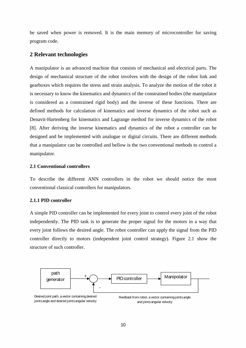
A simple PID controller can be implemented for every joint to control every joint of the robot

independently. The PID task is to generate the proper signal for the motors in a way that

every joint follows the desired angle. The robot controller can apply the signal from the PID

controller directly to motors (independent joint control strategy). Figure 2.1 show the

structure of such controller.

Manipolator path

generator PID controller

-

+

Feedback from robot, a vector containing joints angle and joints angular velocity

Desired joint path, a vector containing desired joints angle and desired joints angular velocity

11

Figure 2.1 PID controller with independent joint control strategy

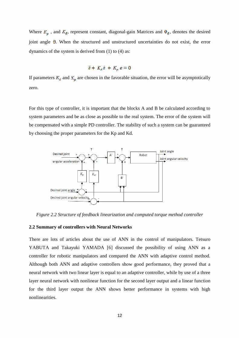
2.1.2 Computed torque method

The PID controller is not an efficient controller to control a manipulator because the

torques output signal that is generated by the PID controller is not dependant on the other

joints. The motion of the other links may apply considerable torque and force to the joint.

This unpredicted torque may not be compensated with the PID controller therefore the

performance of the controller drops when the robot performs in high speeds, a much better

method to control the robot is to calculate the inverse dynamics of the robot and consider the

computed torques to generate control signal. By this method the robot performs well even in

high speeds. The problem with this controller is that in order to calculate the inverse

dynamics of the robot its parameters must be determined and very nonlinear equations should

be solved. Feedback linearization method is one of the most common methods for controlling

a robot and is widely used in the industry.

To describe more a robot consists of a set of moving rigid links which are connected in a

serial chain and its motion equation is given by

T= M( )u + h( , ) (1)

Where,

T represents the vector of joint torques supplied by the actuators. M and h are manipulator

inertia matrix and the vector of the centrifugal and Coriolis terms respectively. , and

are respectively, vectors of joint angles, angular velocities, and angular accelerations.

The control system with the computed torque method is shown in Figure 2.2. The nonlinear

compensation portion is:

(2)

and are the estimated values of the true parameters M and h, respectively.

The servo portion is

(3)

The servo error e is defined as:

(4)

12

Where , and , represent constant, diagonal-gain Matrices and , denotes the desired

joint angle . When the structured and unstructured uncertainties do not exist, the error

dynamics of the system is derived from (1) to (4) as:

If parameters and are chosen in the favorable situation, the error will be asymptotically

zero.

For this type of controller, it is important that the blocks A and B be calculated according to

system parameters and be as close as possible to the real system. The error of the system will

be compensated with a simple PD controller. The stability of such a system can be guaranteed

by choosing the proper parameters for the Kp and Kd.

Figure 2.2 Structure of feedback linearization and computed torque method controller

2.2 Summary of controllers with Neural Networks

There are lots of articles about the use of ANN in the control of manipulators. Tetsuro

YABUTA and Takayuki YAMADA [6] discussed the possibility of using ANN as a

controller for robotic manipulators and compared the ANN with adaptive control method.

Although both ANN and adaptive controllers show good performance, they proved that a

neural network with two linear layer is equal to an adaptive controller, while by use of a three

layer neural network with nonlinear function for the second layer output and a linear function

for the third layer output the ANN shows better performance in systems with high

nonlinearities.

13

In [9] there is a good comparison of different ANN structures as a controller for a three DOF

robot manipulator. Feed forward Neural Networks (FNN), Radial Basis Function Neural

Networks (RBFNN), Runge-Kutta Neural Networks (RKNN) and Adaptive Neuro Fuzzy

Inference Systems (ANFIS) are compared to each other and different learning methods are

evaluated.

There are different approaches for implementation of controllers using ANN. The simplest

structure is introduced in [1]. In this approach first the network is trained with samples from

model of robot and after the convergence of robot output is guaranteed, the model is replaced

with real system and the robot trains in real-time in order to adapt to the real system. By

using such approach we don’t need to calculate the inverse dynamics of the system and

implementation is easy however by changing the desired trajectory we have to train the robot

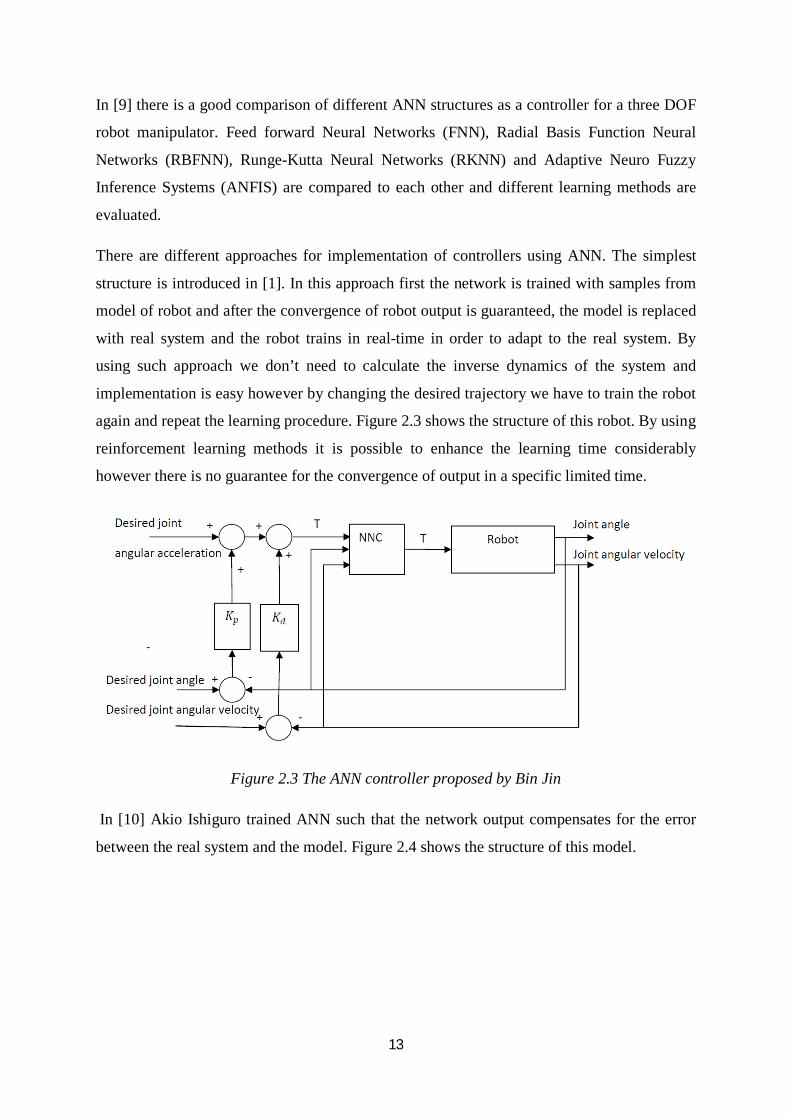
again and repeat the learning procedure. Figure 2.3 shows the structure of this robot. By using

reinforcement learning methods it is possible to enhance the learning time considerably

however there is no guarantee for the convergence of output in a specific limited time.

Figure 2.3 The ANN controller proposed by Bin Jin

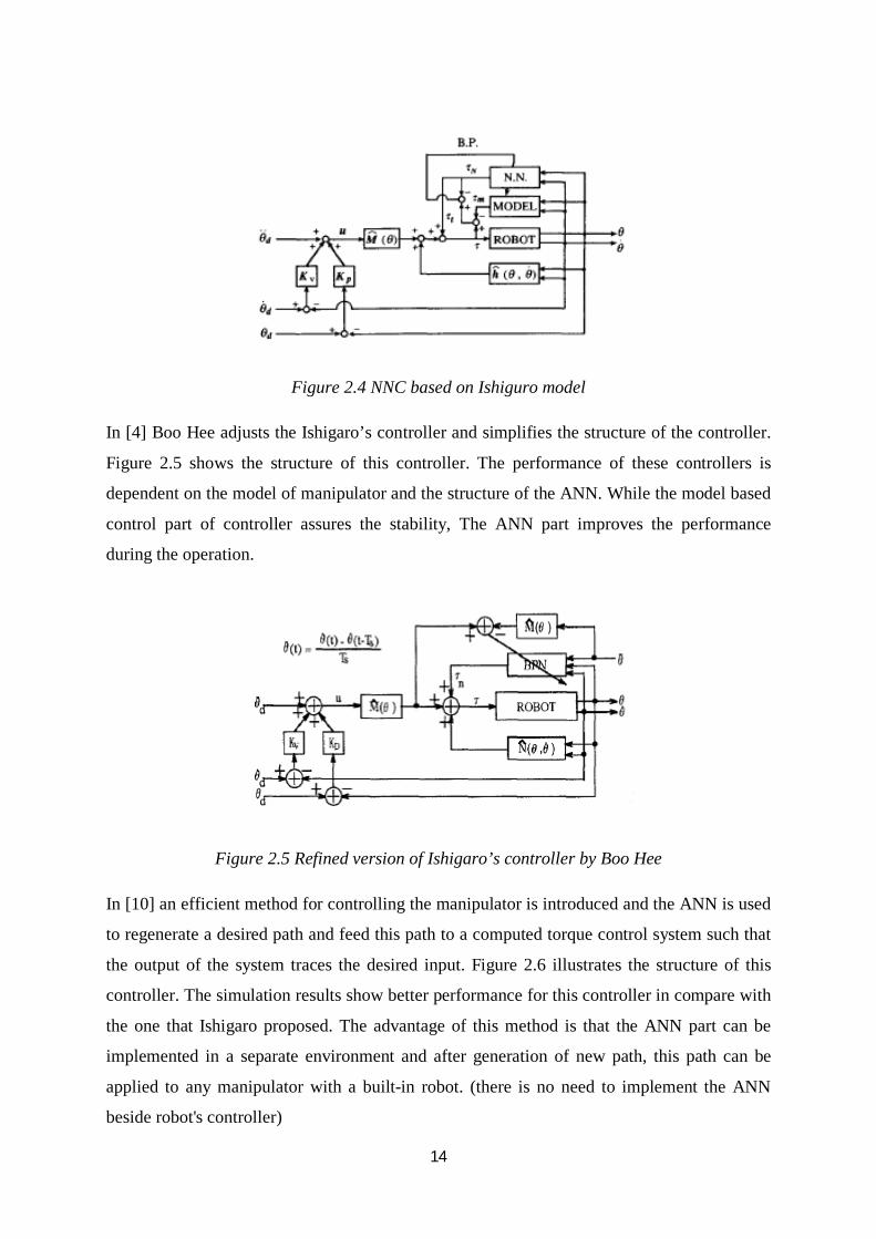
In [10] Akio Ishiguro trained ANN such that the network output compensates for the error

between the real system and the model. Figure 2.4 shows the structure of this model.

14

Figure 2.4 NNC based on Ishiguro model

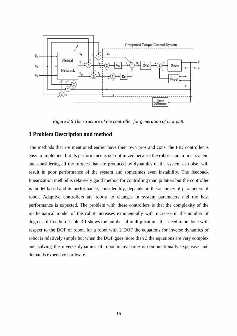
In [4] Boo Hee adjusts the Ishigaro’s controller and simplifies the structure of the controller.

Figure 2.5 shows the structure of this controller. The performance of these controllers is

dependent on the model of manipulator and the structure of the ANN. While the model based

control part of controller assures the stability, The ANN part improves the performance

during the operation.

Figure 2.5 Refined version of Ishigaro’s controller by Boo Hee

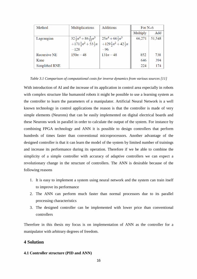
In [10] an efficient method for controlling the manipulator is introduced and the ANN is used

to regenerate a desired path and feed this path to a computed torque control system such that

the output of the system traces the desired input. Figure 2.6 illustrates the structure of this

controller. The simulation results show better performance for this controller in compare with

the one that Ishigaro proposed. The advantage of this method is that the ANN part can be

implemented in a separate environment and after generation of new path, this path can be

applied to any manipulator with a built-in robot. (there is no need to implement the ANN

beside robot's controller)

15

Figure 2.6 The structure of the controller for generation of new path

3 Problem Description and method

The methods that are mentioned earlier have their own pros and cons. the PID controller is

easy to implement but its performance is not optimized because the robot is not a liner system

and considering all the torques that are produced by dynamics of the system as noise, will

result in poor performance of the system and sometimes even instability. The feedback

linearization method is relatively good method for controlling manipulators but the controller

is model based and its performance, considerably, depends on the accuracy of parameters of

robot. Adaptive controllers are robust to changes in system parameters and the best

performance is expected. The problem with these controllers is that the complexity of the

mathematical model of the robot increases exponentially with increase in the number of

degrees of freedom. Table 3.1 shows the number of multiplications that need to be done with

respect to the DOF of robot. for a robot with 2 DOF the equations for inverse dynamics of

robot is relatively simple but when the DOF goes more than 3 the equations are very complex

and solving the inverse dynamics of robot in real-time is computationally expensive and

demands expensive hardware.

16

Table 3.1 Comparison of computational costs for inverse dynamics from various sources [11]

With introduction of AI and the increase of its application in control area especially in robots

with complex structure like humanoid robots it might be possible to use a learning system as

the controller to learn the parameters of a manipulator. Artificial Neural Network is a well

known technology in control applications the reason is that the controller is made of very

simple elements (Neurons) that can be easily implemented on digital electrical boards and

these Neurons work in parallel in order to calculate the output of the system. For instance by

combining FPGA technology and ANN it is possible to design controllers that perform

hundreds of times faster than conventional microprocessors. Another advantage of the

designed controller is that it can learn the model of the system by limited number of trainings

and increase its performance during its operation. Therefore if we be able to combine the

simplicity of a simple controller with accuracy of adaptive controllers we can expect a

revolutionary change in the structure of controllers. The ANN is desirable because of the

following reasons

1. It is easy to implement a system using neural network and the system can train itself

to improve its performance

2. The ANN can perform much faster than normal processors due to its parallel

processing characteristics

3. The designed controller can be implemented with lower price than conventional

controllers

Therefore in this thesis my focus is on implementation of ANN as the controller for a

manipulator with arbitrary degrees of freedom.

4 Solution

4.1 Controller structure (PID and ANN)

17

The problem for the ANN is to solve the inverse dynamics of the system. In order to train the

ANN to learn this function it is possible to train it with random data or use a controller to

provide good samples for training the ANN. In other words the ANN can work alone as the

controller or it can be used in parallel with other controllers. The idea is to construct a

controller with the simplest structure and observe the performance of the system. If the

results are not satisfactory then increase the complexity of controller (use the model based

control and decrease the complexity of the problem that ANN should solve) and simplify the

problem that the ANN has to solve.

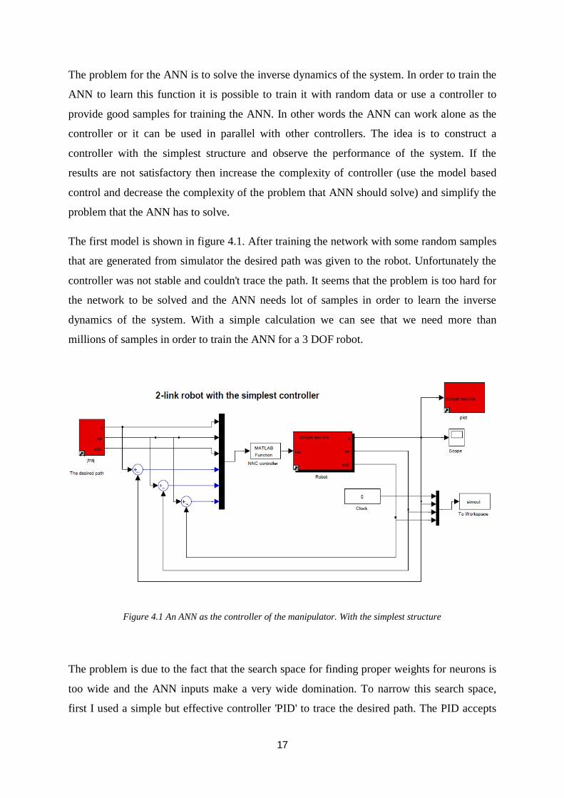
The first model is shown in figure 4.1. After training the network with some random samples

that are generated from simulator the desired path was given to the robot. Unfortunately the

controller was not stable and couldn't trace the path. It seems that the problem is too hard for

the network to be solved and the ANN needs lot of samples in order to learn the inverse

dynamics of the system. With a simple calculation we can see that we need more than

millions of samples in order to train the ANN for a 3 DOF robot.

Figure 4.1 An ANN as the controller of the manipulator. With the simplest structure

The problem is due to the fact that the search space for finding proper weights for neurons is

too wide and the ANN inputs make a very wide domination. To narrow this search space,

first I used a simple but effective controller 'PID' to trace the desired path. The PID accepts

18

the angle and angular velocities of the joints and generates the required torque for the motors.

Although this controller cannot perform well and the error is not within satisfactory range,

the data which are collected from the PID are good samples for training the ANN. After

training the ANN with sample data from PID the ANN is used as a controller in parallel to

PID and new samples for training are generated.

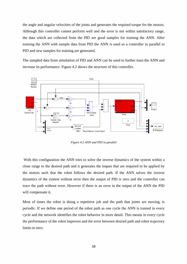
The sampled data from simulation of PID and ANN can be used to further train the ANN and

increase its performance. Figure 4.2 shows the structure of this controller.

Figure 4.2 ANN and PID in parallel

With this configuration the ANN tries to solve the inverse dynamics of the system within a

close range to the desired path and it generates the toques that are required to be applied by

the motors such that the robot follows the desired path. If the ANN solves the inverse

dynamics of the system without error then the output of PID is zero and the controller can

trace the path without error. However if there is an error in the output of the ANN the PID

will compensate it.

Most of times the robot is doing a repetitive job and the path that joints are moving, is

periodic. If we define one period of the robot path as one cycle the ANN is trained in every

cycle and the network identifies the robot behavior in more detail. This means in every cycle

the performance of the robot improves and the error between desired path and robot trajectory

limits to zero.

19

After implementation of the system and simulation, simulation results shows that the error

converges to zero and it can be reduced to arbitrary value with enough number of trainings.

4.1.1 ANN structure

4.1.1.1 Inputs and outputs

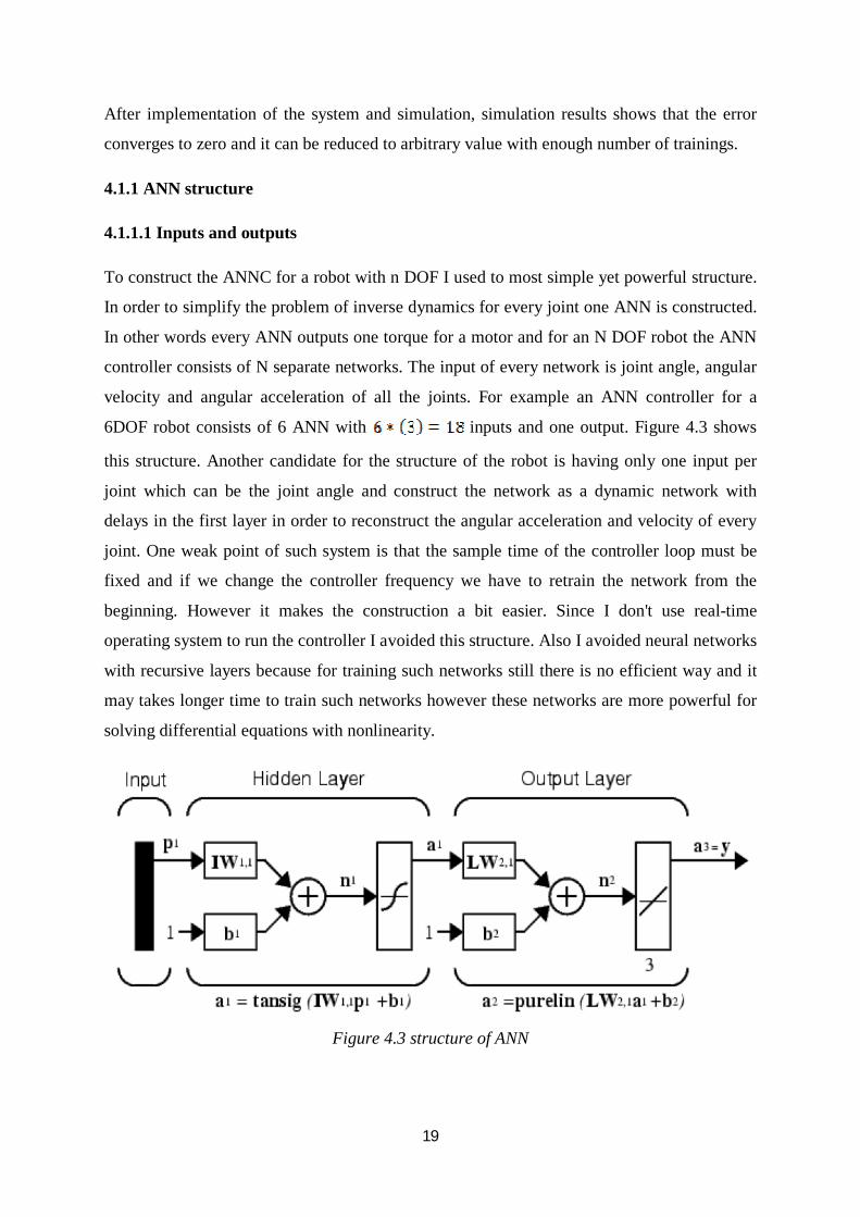
To construct the ANNC for a robot with n DOF I used to most simple yet powerful structure.

In order to simplify the problem of inverse dynamics for every joint one ANN is constructed.

In other words every ANN outputs one torque for a motor and for an N DOF robot the ANN

controller consists of N separate networks. The input of every network is joint angle, angular

velocity and angular acceleration of all the joints. For example an ANN controller for a

6DOF robot consists of 6 ANN with inputs and one output. Figure 4.3 shows

this structure. Another candidate for the structure of the robot is having only one input per

joint which can be the joint angle and construct the network as a dynamic network with

delays in the first layer in order to reconstruct the angular acceleration and velocity of every

joint. One weak point of such system is that the sample time of the controller loop must be

fixed and if we change the controller frequency we have to retrain the network from the

beginning. However it makes the construction a bit easier. Since I don't use real-time

operating system to run the controller I avoided this structure. Also I avoided neural networks

with recursive layers because for training such networks still there is no efficient way and it

may takes longer time to train such networks however these networks are more powerful for

solving differential equations with nonlinearity.

Figure 4.3 structure of ANN

20

4.1.1.2 Network structure

Every ANN is consists of two hidden layer which the first layer output function is the

sigmoid function and the second layer output function is a linear function, figure 4.3. It is

proven that a network with this structure and enough amounts of neurons in its hidden layer

can produce any function with limited number of discontinuity.

4.1.2 Training method

The problem that the network must solve is the inverse dynamics of the system which can be

presented as a simple function, y=F(x), where x is a vector with values of zero, first and

second derivative of joint angles and y is a toque vector that is applied to joints. To train the

network we must provide the ANN with a pair of [x y]. As mentioned earlier the ANN is

trained with the data which is generated by PID controller such that when the PID generated

the torque [Ti] this torque is applied to the robot with the joint angles of vector [Ji] and

angular velocities of [Wi] and then the acceleration is measured as a vector of [Ai]. In this

way the pair of [x y ] for training the network is achieved by putting x=[Ji, Wi, Ai], y=[Ti].

In other words we get the data from the forward dynamics of the system which is solved by

simulator or the real robot and use this data to solve the inverse dynamics of the system.

After gathering data from one cycle of robot operation the whole network is trained in the

back propagation mode and all the weighs are updated according to the new tainting data. In

the simulation both the incremental learning and Back Learning is used but the incremental

learning is very slow and more often the weights are trapped in the local minimums.

4.1.2.1 Learning function

The training function is the "Trainlm" function from MATLAB toolbox. Trainlm is a network

training function that updates weight and bias values according to Levenberg-Marquardt

optimization [12]. It is often the fastest back propagation algorithm in the Matlab toolbox,

and is highly recommended as a first-choice supervised algorithm, although it does require

more memory than other algorithms. Back propagation is used to calculate the Jacobian of

performance with respect to the weight and bias. For more information about Trainlm see

[13]

21

5 Simulations

5.1 Simulator environment

The simulation is done in Matlab and Matlab robotics toolbox from Peter I. Corke [11]. The

toolbox has several useful simulink models that are accompanied by M-files to do the

simulation and modeling.

5.2 Robotic toolbox

The Toolbox is an open source toolbox for Matlab and provides many functions that are

useful in robotics such as trajectory generator and functions for solving kinematics, dynamics

and inverse of them. The Toolbox is useful for simulation as well as analyzing results from

experiments with real robots. The Toolbox is based on a very general method of representing

the kinematics and dynamics of serial-link manipulators. The useful functions in the toolbox

are: link, robot, ikin, fkine, accel, puma and twolink (functions for defining and computing

the robot kinematics and dynamics respectively), the commands puma560 and two link

automatically construct a puma560 and a simple two link robot, the parameters of the

puma560 robot object are derived from the parameters of the real manipulator 'Puma560' and

the results of the simulation is compared to the real robot. For details about the robotic

toolbox see [11]

5.3 A simulator with symbolic toolbox

To testify the accuracy of the simulator I wrote the equation for the inverse dynamics of the

robot and solved the equations by the Matlab symbolic toolbox. A simple 6DOF robot was

made and the simulation was tested on the robot to assure the accuracy of the robotics

toolbox.

5.4 Simulation results

The ANN is designed in MATLAB Simulink environment and tested with simulator from

Matlab Robotics Toolbox. Two robots used to testify the performance of the controller. First

robot is a two DOF robot and second robot is a puma560. The parameters for this 6DOF

robot are extracted from real robot PUMA560.

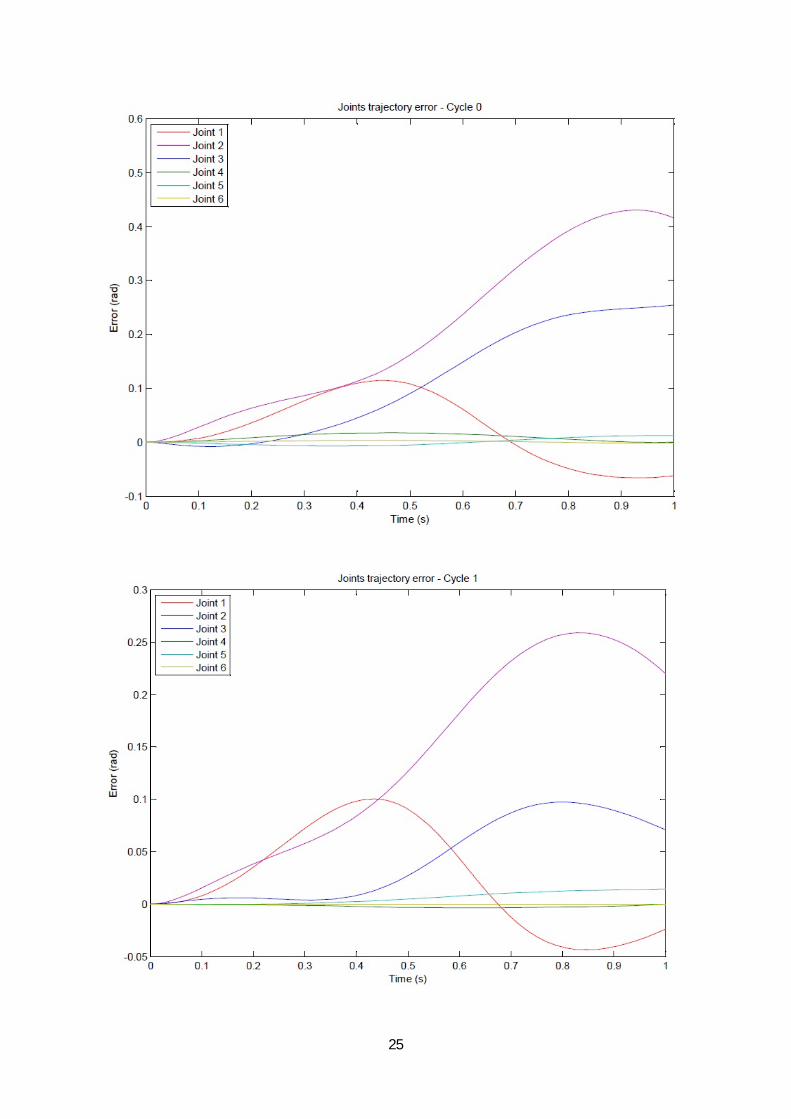
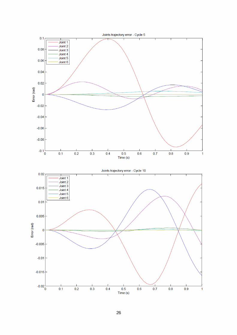
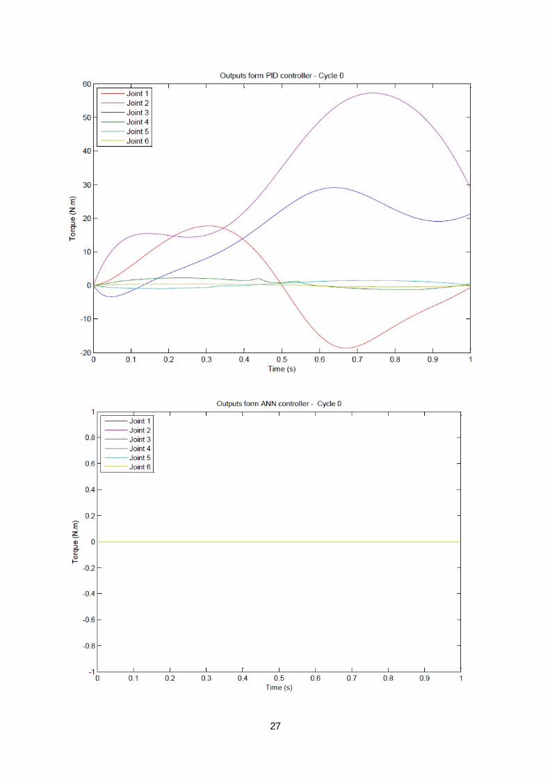
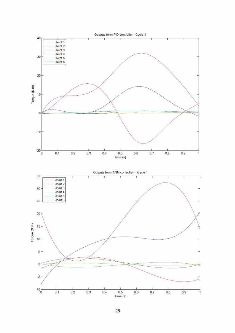
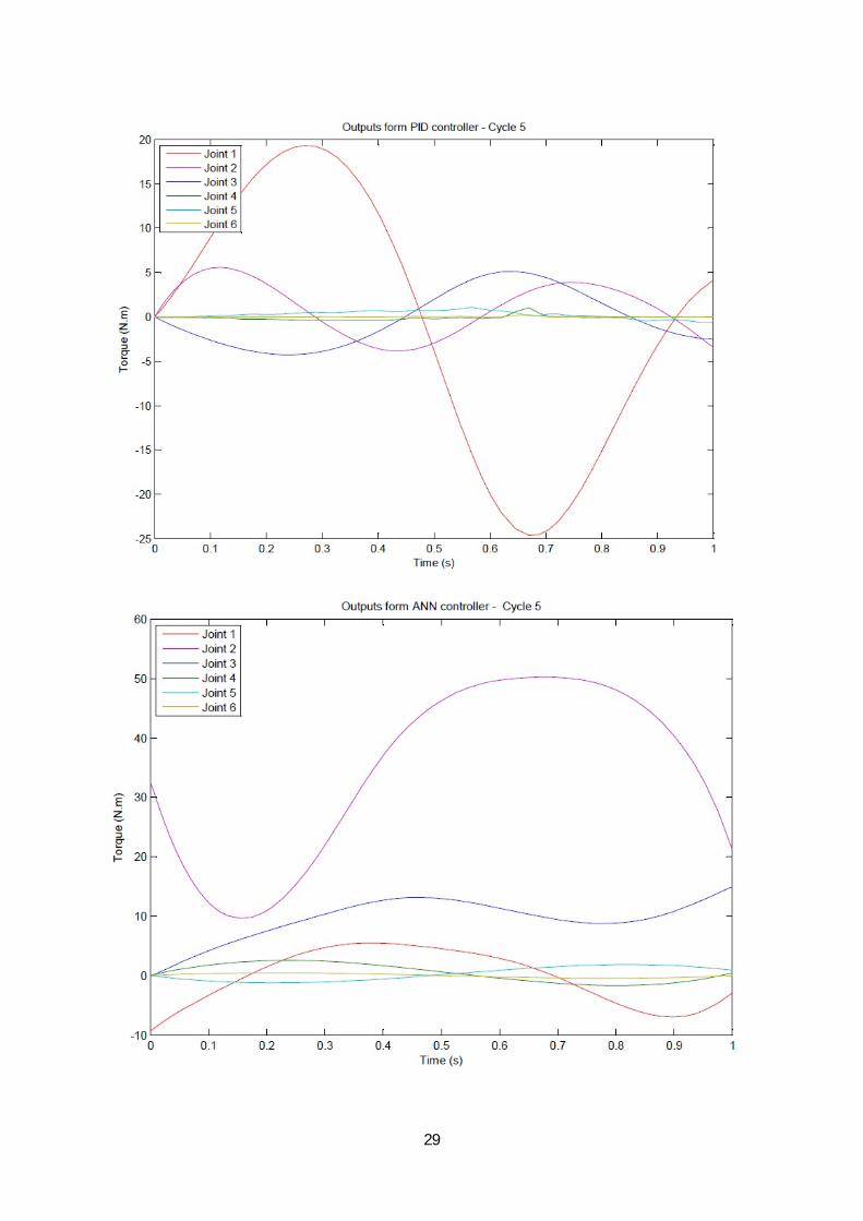
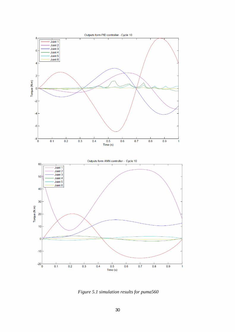
The motion of robot between two points in joint space is illustrated in the figure 5.1. Robot

path is generated by the 'jtraj' Function from the robotic toolbox [11] and is a polynomial to

22

the order of 5. The values for the PID controller are . In the

graphs the trajectory path of the robot as well as error of the controller (the error between

desired path and robot path) is shown. The other graphs show a comparison between the

output of PID part of the controller and the output of ANN. It is shown that as the training

continues the PID output reduces and the ANN generates the main signal for the robot

control.

As it is obvious in the system the network solves the inverse dynamics of the system very fast

and a significant improvement is observed after the first cycle of training.

The number of neurons in the network may affect the performance of the system and as the

number of neurons increases the error of the system decreases however the network needs

more training data. One idea is that at the first cycles of training the network is constructed

with a few neurons and as the training continues newer networks with more neurons be be

substituted with previous networks to achieve better performance.

23

24

25

26

27

28

29

30

Figure 5.1 simulation results for puma560

31

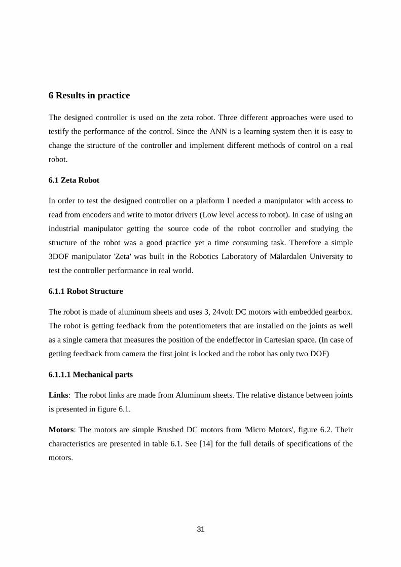
6 Results in practice

The designed controller is used on the zeta robot. Three different approaches were used to

testify the performance of the control. Since the ANN is a learning system then it is easy to

change the structure of the controller and implement different methods of control on a real

robot.

6.1 Zeta Robot

In order to test the designed controller on a platform I needed a manipulator with access to

read from encoders and write to motor drivers (Low level access to robot). In case of using an

industrial manipulator getting the source code of the robot controller and studying the

structure of the robot was a good practice yet a time consuming task. Therefore a simple

3DOF manipulator 'Zeta' was built in the Robotics Laboratory of Mälardalen University to

test the controller performance in real world.

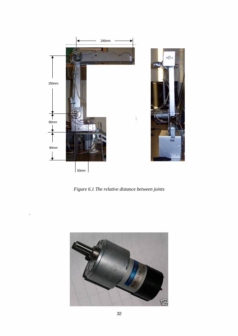
6.1.1 Robot Structure

The robot is made of aluminum sheets and uses 3, 24volt DC motors with embedded gearbox.

The robot is getting feedback from the potentiometers that are installed on the joints as well

as a single camera that measures the position of the endeffector in Cartesian space. (In case of

getting feedback from camera the first joint is locked and the robot has only two DOF)

6.1.1.1 Mechanical parts

Links: The robot links are made from Aluminum sheets. The relative distance between joints

is presented in figure 6.1.

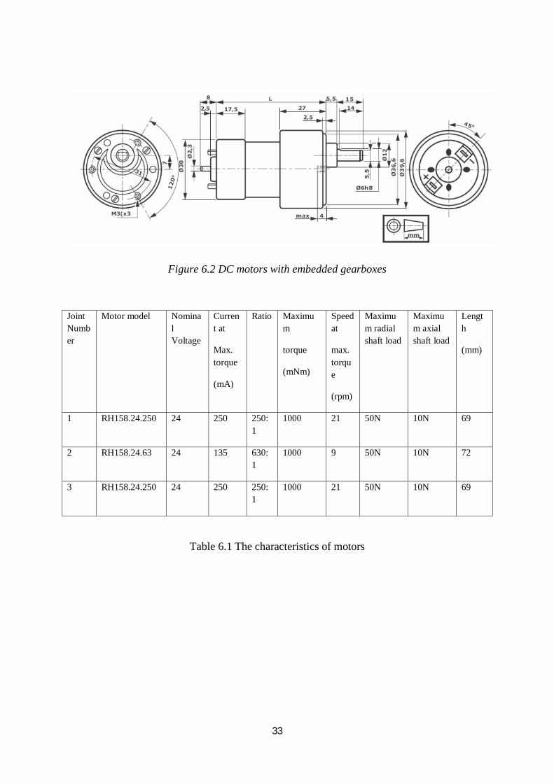
Motors: The motors are simple Brushed DC motors from 'Micro Motors', figure 6.2. Their

characteristics are presented in table 6.1. See [14] for the full details of specifications of the

motors.

32

Figure 6.1 The relative distance between joints

.

245mm

80mm

250mm

50mm

90mm

33

Figure 6.2 DC motors with embedded gearboxes

Joint Number

Motor model Nominal Voltage

Current at

Max. torque

(mA)

Ratio Maximum

torque

(mNm)

Speed at

max. torque

(rpm)

Maximum radial shaft load

Maximum axial shaft load

Length

(mm)

1 RH158.24.250 24 250 250:1

1000 21 50N 10N 69

2 RH158.24.63 24 135 630:1

1000 9 50N 10N 72

3 RH158.24.250 24 250 250:1

1000 21 50N 10N 69

Table 6.1 The characteristics of motors

34

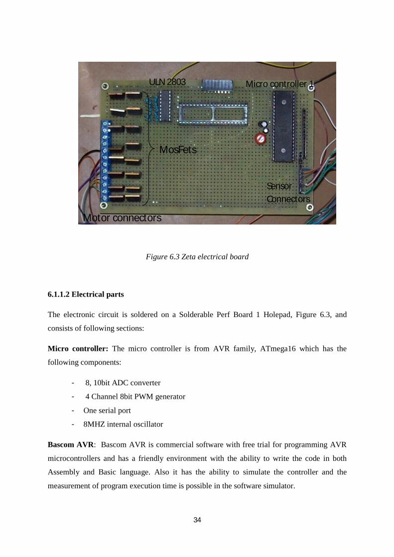
Figure 6.3 Zeta electrical board

6.1.1.2 Electrical parts

The electronic circuit is soldered on a Solderable Perf Board 1 Holepad, Figure 6.3, and

consists of following sections:

Micro controller: The micro controller is from AVR family, ATmega16 which has the

following components:

- 8, 10bit ADC converter

- 4 Channel 8bit PWM generator

- One serial port

- 8MHZ internal oscillator

Bascom AVR: Bascom AVR is commercial software with free trial for programming AVR

microcontrollers and has a friendly environment with the ability to write the code in both

Assembly and Basic language. Also it has the ability to simulate the controller and the

measurement of program execution time is possible in the software simulator.

Motor connectors

MosFets

Micro controller 1 ULN 2803

Sensor Connectors

35

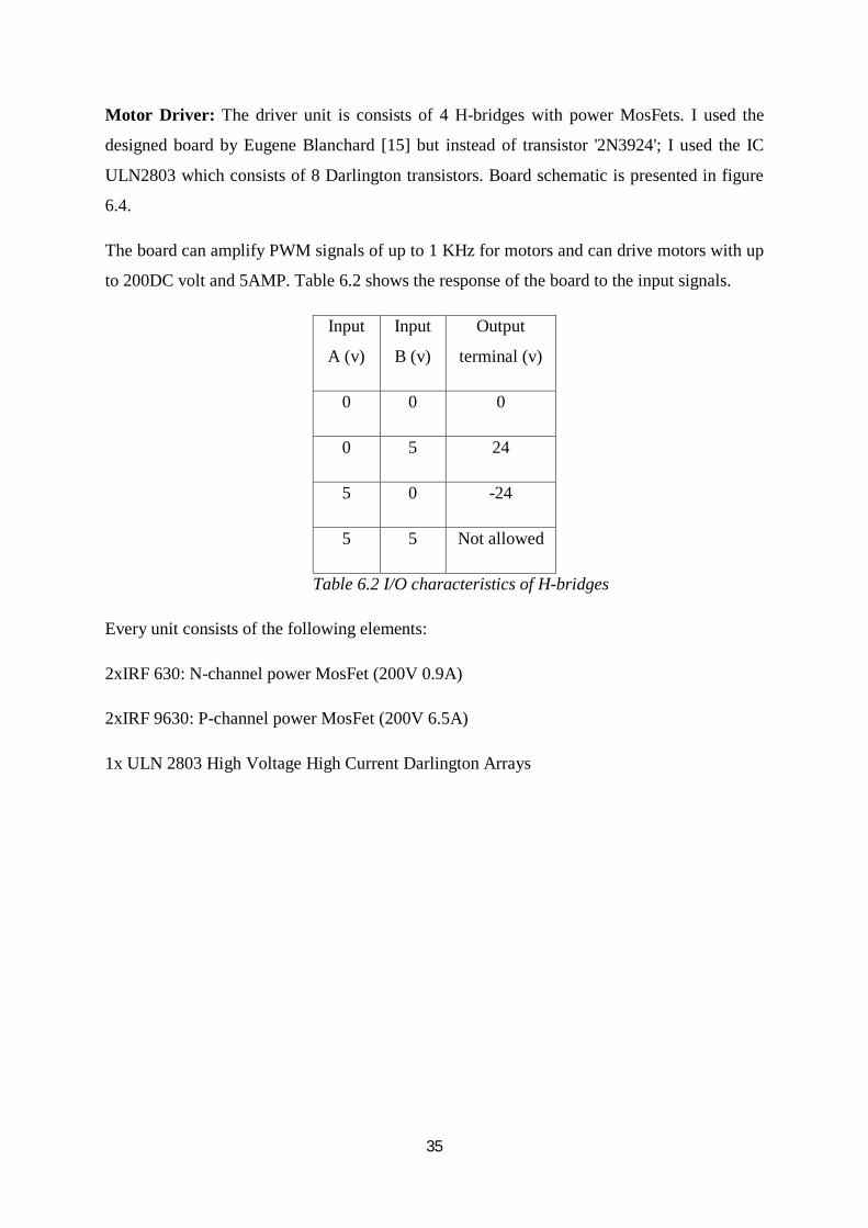
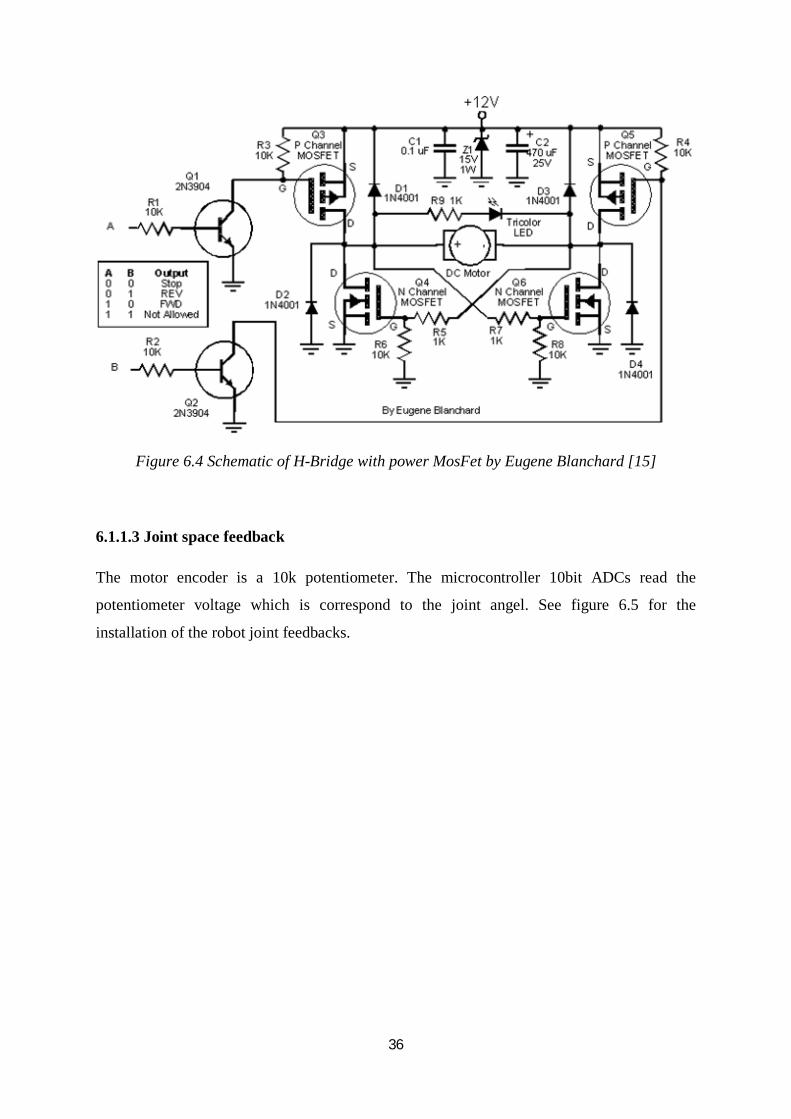
Motor Driver: The driver unit is consists of 4 H-bridges with power MosFets. I used the

designed board by Eugene Blanchard [15] but instead of transistor '2N3924'; I used the IC

ULN2803 which consists of 8 Darlington transistors. Board schematic is presented in figure

6.4.

The board can amplify PWM signals of up to 1 KHz for motors and can drive motors with up

to 200DC volt and 5AMP. Table 6.2 shows the response of the board to the input signals.

Input

A (v)

Input

B (v)

Output

terminal (v)

0 0 0

0 5 24

5 0 -24

5 5 Not allowed

Table 6.2 I/O characteristics of H-bridges

Every unit consists of the following elements:

2xIRF 630: N-channel power MosFet (200V 0.9A)

2xIRF 9630: P-channel power MosFet (200V 6.5A)

1x ULN 2803 High Voltage High Current Darlington Arrays

36

Figure 6.4 Schematic of H-Bridge with power MosFet by Eugene Blanchard [15]

6.1.1.3 Joint space feedback

The motor encoder is a 10k potentiometer. The microcontroller 10bit ADCs read the

potentiometer voltage which is correspond to the joint angel. See figure 6.5 for the

installation of the robot joint feedbacks.

37

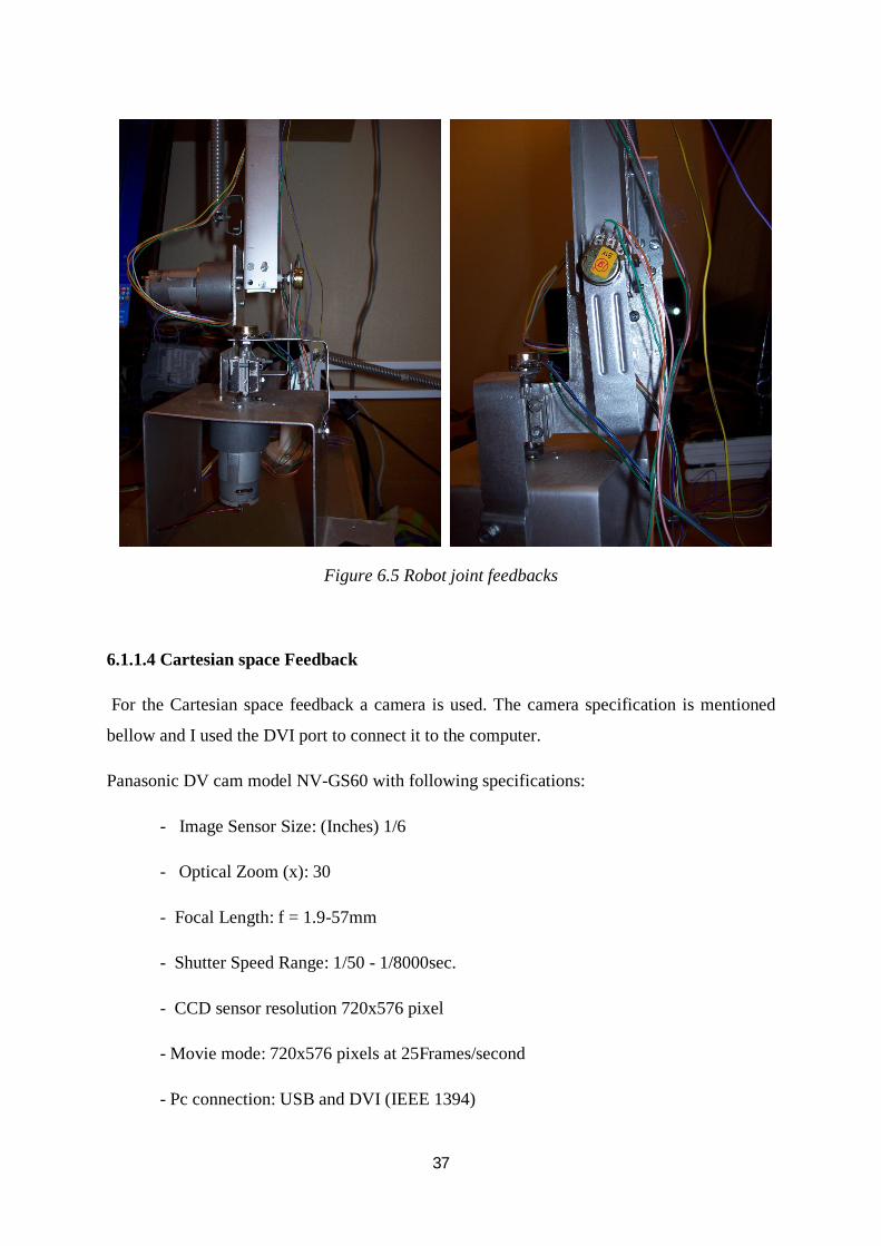
Figure 6.5 Robot joint feedbacks

6.1.1.4 Cartesian space Feedback

For the Cartesian space feedback a camera is used. The camera specification is mentioned

bellow and I used the DVI port to connect it to the computer.

Panasonic DV cam model NV-GS60 with following specifications:

- Image Sensor Size: (Inches) 1/6

- Optical Zoom (x): 30

- Focal Length: f = 1.9-57mm

- Shutter Speed Range: 1/50 - 1/8000sec.

- CCD sensor resolution 720x576 pixel

- Movie mode: 720x576 pixels at 25Frames/second

- Pc connection: USB and DVI (IEEE 1394)

38

6.2 Zeta robot operation

6.2.1 Microcontroller operation

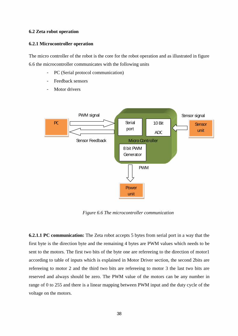
The micro controller of the robot is the core for the robot operation and as illustrated in figure

6.6 the microcontroller communicates with the following units

- PC (Serial protocol communication)

- Feedback sensors

- Motor drivers

Figure 6.6 The microcontroller communication

6.2.1.1 PC communication: The Zeta robot accepts 5 bytes from serial port in a way that the

first byte is the direction byte and the remaining 4 bytes are PWM values which needs to be

sent to the motors. The first two bits of the byte one are refereeing to the direction of motor1

according to table of inputs which is explained in Motor Driver section, the second 2bits are

refereeing to motor 2 and the third two bits are refereeing to motor 3 the last two bits are

reserved and always should be zero. The PWM value of the motors can be any number in

range of 0 to 255 and there is a linear mapping between PWM input and the duty cycle of the

voltage on the motors.

PWM

Micro Controller

Serial port

PC Sensor unit

Power unit

PWM signal

Sensor Feedback

Sensor signal

10 Bit

ADC

8 bit PWM Generator

39

After start of the robot the micro controller waits for the PWM signal and after the PWM

value is received the microcontroller gets the joint position from the feedback sensors and

sends it to the serial port as 5, 16bit, numbers with the following order: the first byte is the

absolute time of capturing data. The second, third and fourth numbers are the values received

from the joint 1 to 3. The 5th byte is reserved for future use and is always 0. After the data is

sent via serial port the robot goes to the start of the loop and awaits for the PWM data from

serial port.

6.2.1.2 Capturing ADC data

The ADCs are configured to get the data from the adc0 to adc3 pins of the micro controller

and the ADC reference voltage is set to 5 volts. For the noise reduction of the analog circuit a

second order LC filter is placed between the analog VCC and digital VCC. At the start of the

robot the microcontroller timer 1 is configured to count the CPU cycles and when the data is

captured from the ADC's the CPU time in term of timer1 cycles is attached to the sensor data.

This time stamp helps the robot controller to estimate the current position of the robot and

can increase the performance of the controller in the case of using a non-real-time operating

system.

6.2.1.3 PWM generation

I wrote two different codes for generation of the PWM signal. The first code uses only one

timer of the micro controller and there is no limit for the number of PWM generation,

however the CPU utilization increases exponentially with the number of PWM productions

and it may happen that in some cases the PWM signal doesn't have the right shape. This code

can generate a PWM signal for 4 motors up to frequency of 200 Hz when the microcontroller

is working at 8MHZ frequency. The algorithm for code is such that after the PWM value are

received from the controller, these values are sorted in a table and the program interrupts the

microcontroller CPU whenever one of the values of this table is matched with the timer 1

register.

The second code uses all three timers of the ATmega16 and can generate PWM for up to

4motors. The PWM jitter is lower and the PWM frequency can go up to 2Khz. In this case

the microcontroller timers are configured to work as Compare-Match timers and whenever

the PWM value of motor is equal to the timer value an interrupt accurse and proper signal is

generated.

40

6.2.2 Cartesian space feedback

6.2.2.1 Tracking point

There are different methods that can be used to track the endeffector, depending on the type

of endeffector object detection may be a time consuming task and it involves advanced

techniques in machine vision topic. Besides the lot of code that has to be written, the image

processing is a heavy task for current CPU's and for real-time computation it requires

expensive hardware, therefore I used an object on the robot as the tracking point 'A red LED'.

The LED is installed on the third link of the robot and its head is pointed to the camera.

Finding this point in the scene is a very simple task and the error of position determination is

very low.

6.2.2.2 Camera connection

The camera is connected to PC via DVI port (IEEE 1394 protocol) and Matlab recognizes the

camera as a standard image capturing device.

6.2.2.3 Offline image processing

For the offline image processing the trigger signal was set to manual and the number of

images per trigger was set to 300. The camera can capture 720x576 pixels pictures at 25

frames/s. This means that after generation of the trigger signal from the PC, the pictures will

be logged to memory every 40ms and since the camera has its own embedded system and the

scene is not changing I expect the real-time performance of taking pictures. A good point is

that although Windows does not have real-time performance but the image capturing task is

in real-time, the data is buffered in the camera memory and is sent to the PC via firewire

cable, within this transfer there may be unknown delays but since the image processing is

done offline, these delays wont effect the performance of the controller. After the pictures are

captured from camera and saved into computer memory, they are captured from camera objet

and the image processing is done in offline mode.

With automatic settings in the camera the red LED looks like a shiny white light in the

pictures therefore in order to decrease the noise in the systems and have the best performance

I switched the camera operation to manual mode and set the shutter speed to 1/8000 second

41

and set the gain to 12dB. Also I disabled the autofocus function to avoid the errors of changes

in the sharpness of the pictures.

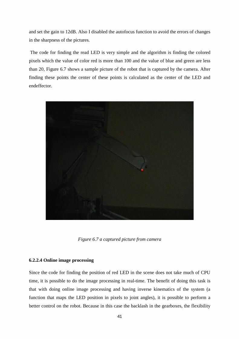
The code for finding the read LED is very simple and the algorithm is finding the colored

pixels which the value of color red is more than 100 and the value of blue and green are less

than 20, Figure 6.7 shows a sample picture of the robot that is captured by the camera. After

finding these points the center of these points is calculated as the center of the LED and

endeffector.

Figure 6.7 a captured picture from camera

6.2.2.4 Online image processing

Since the code for finding the position of red LED in the scene does not take much of CPU

time, it is possible to do the image processing in real-time. The benefit of doing this task is

that with doing online image processing and having inverse kinematics of the system (a

function that maps the LED position in pixels to joint angles), it is possible to perform a

better control on the robot. Because in this case the backlash in the gearboxes, the flexibility

42

of the links and offset in the joints feedback sensor won't affect the calculations for finding

the position of endeffector.

It is possible that in Matlab, assign the task of image processing to one CPU and with the

other CPU do the controller task (parallel processing is possible only if the PC processor have

multi cores).

A good consideration in doing online image processing is that after running the camera the

pictures are taken by the camera and when the PC sends the trigger signal, the data in buffer

will be returned by the camera. In other words it in not possible to change the frame rate of

camera to a desired value and the only possible thing is to drop some frames. In the case that

the computer processor is slow and the controller drops some frames it is good to notice the

fact that the relative time between capturing the frames is multiply of 40ms.

The algorithm for calculating the LED position is same as offline processing but it is possible

to neglect the calculation of the blue and green colors Since the other pixels in the picture are

relatively dark (their value is less than 20 out of 255).

6.3 Controller operation

The controller for the robot consists of a PID controller and a feed forwarded Artificial

Neural Network controller.

6.3.1 Software

In order to control the robot in real-time there are two proposed options:

1. Since the ANN controller output can be generated in offline mode the output signal

can be saved on the microcontroller ROM and since the PID can be easily

implemented in the microcontroller, one easy way is to detach the microcontroller

from the PC and after uploading the ANN data to the microcontroller run the robot in

real-time. The feedback data from sensors can be stored in an external EEPROM and

transferred to PC for training the network after the operation of the robot.

2. By using the Matlab real-time toolbox It is possible to install a small Kernel from

Matlab software and this kernel gives Matlab the possibility of running simulink

applications in real-time. The procedure is that Matlab compiles the simulink model

to an executable file and runs it on the small Kernel. The installed kernel which runs

in CPU ring zero has the ability to control the interrupts that are coming from

43

windows operating system and lets the executable simulink file to run on the PC with

real-time performance. The simulink in Matlab can communicate with this executable

file and exchanges data in non real-time. Therefore it is possible to run the simulink

model of the controller on real-time and log the data to Matlab environment for

training of the network. Computer standard serial port is defined for Matlab simulink

real-time workshop version 7.6 and above and can be used for this purpose. Please

refer to [16] for more information about Matlab real-time windows target.

6.3.2 Controller with Matlab

Since the focus of the thesis is on the ANN controller itself and not on the real-time

performance of the system I used the simulink environment of the Matlab as the controller

and slowed down the simulator and synchronized it with CPU clock. Since the data which is

used from the joint sensors have time stamp it is possible to estimate the position of the robot

at time of generating the control signal. Even though the controller is not working in real-time

and there are unpredictable delays in control loop I expect acceptable results from the robot

performance.

As mentioned above the robot controller consists of two controllers which are working in

parallel: PID controller and ANN controller. This controller is implemented in the simulink

environment and provides the control signal to the Robot manipulator.

PID controller: The PID controller gets its feedback from joint sensors and outputs the

control signal. The frequency Of PID is 50Htz and the computation is done in Matlab

simulink environment.

ANN controller: since the ANN is a feed forwarded network, the input of the systems is

applied to the ANN and the output is calculated in offline. This offline data is stored in a

variable and the simulink interpolates the network output from the offline data. The ANN

signal is added to the output of PID and is sent to the robot via serial port.

6.3.3 Joint control with joint feedback

The structure of controller for this method is same as simulation. Figure 4.2 shows the

structure of this controller.

The uncertainty in the system and sources of noise and error can be named as:

44

1. The backlash in the gearbox and also in the connection between the robot and the

output shaft of gearbox.

2. Noise of reading data from ADC.

3. Use of non real-time operation system to generate the control signal.

4. Since the angular velocities and accelerations are calculated with derivations from

joint angles with respect to time the noise is amplified in these values.

To reduce the error caused by derivations from joint angles two different filters were

designed:

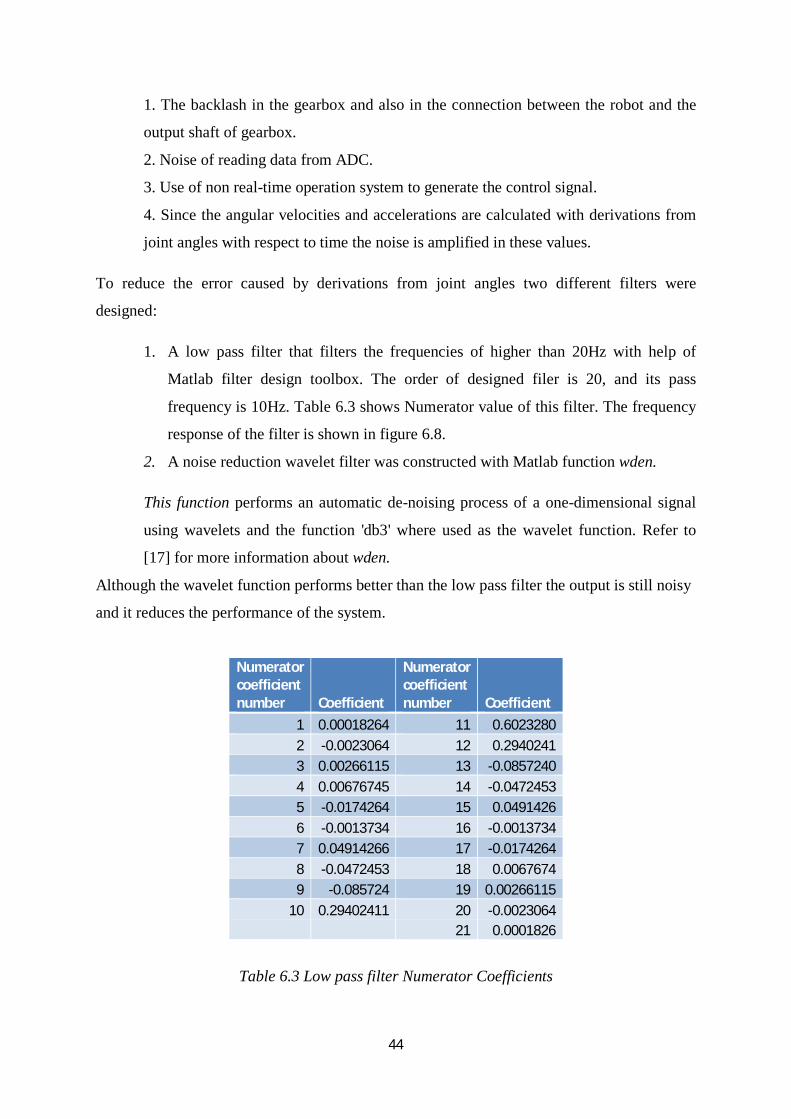
1. A low pass filter that filters the frequencies of higher than 20Hz with help of

Matlab filter design toolbox. The order of designed filer is 20, and its pass

frequency is 10Hz. Table 6.3 shows Numerator value of this filter. The frequency

response of the filter is shown in figure 6.8.

2. A noise reduction wavelet filter was constructed with Matlab function wden.

This function performs an automatic de-noising process of a one-dimensional signal

using wavelets and the function 'db3' where used as the wavelet function. Refer to

[17] for more information about wden.

Although the wavelet function performs better than the low pass filter the output is still noisy

and it reduces the performance of the system.

Numerator coefficient number Coefficient

Numerator coefficient number Coefficient

1 0.00018264 11 0.6023280 2 -0.0023064 12 0.2940241 3 0.00266115 13 -0.0857240 4 0.00676745 14 -0.0472453 5 -0.0174264 15 0.0491426 6 -0.0013734 16 -0.0013734 7 0.04914266 17 -0.0174264 8 -0.0472453 18 0.0067674 9 -0.085724 19 0.00266115

10 0.29402411 20 -0.0023064 21 0.0001826

Table 6.3 Low pass filter Numerator Coefficients

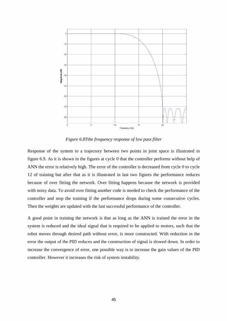
45

Figure 6.8Tthe frequency response of low pass filter

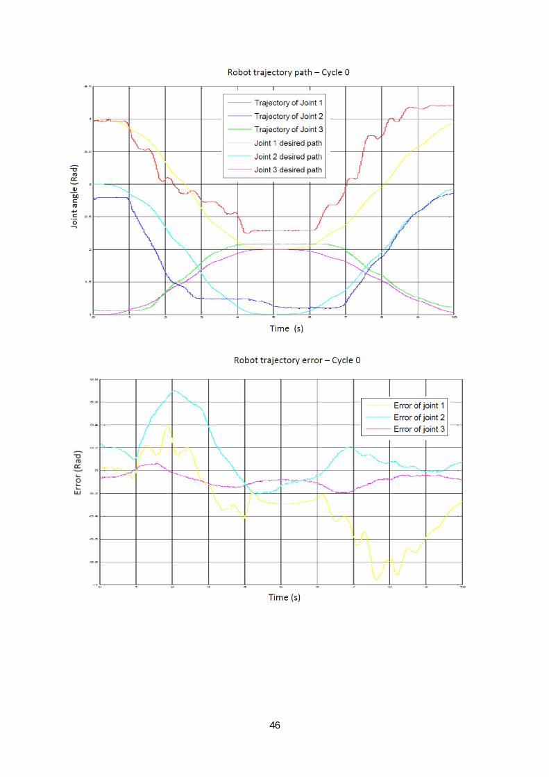
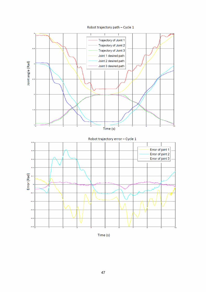
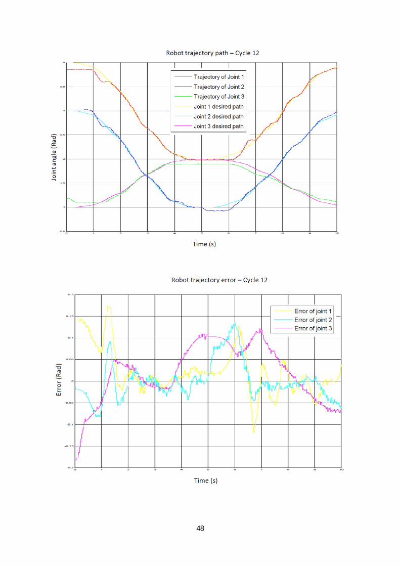
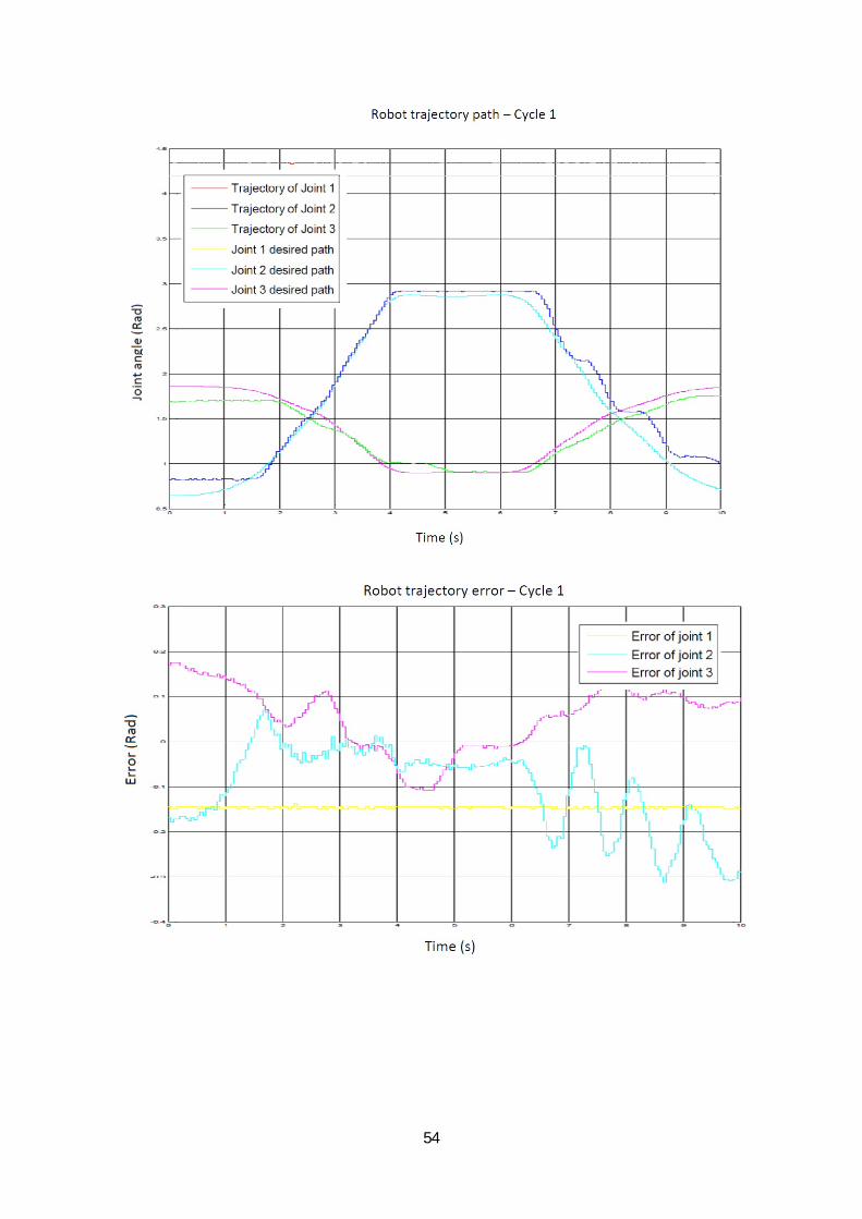
Response of the system to a trajectory between two points in joint space is illustrated in

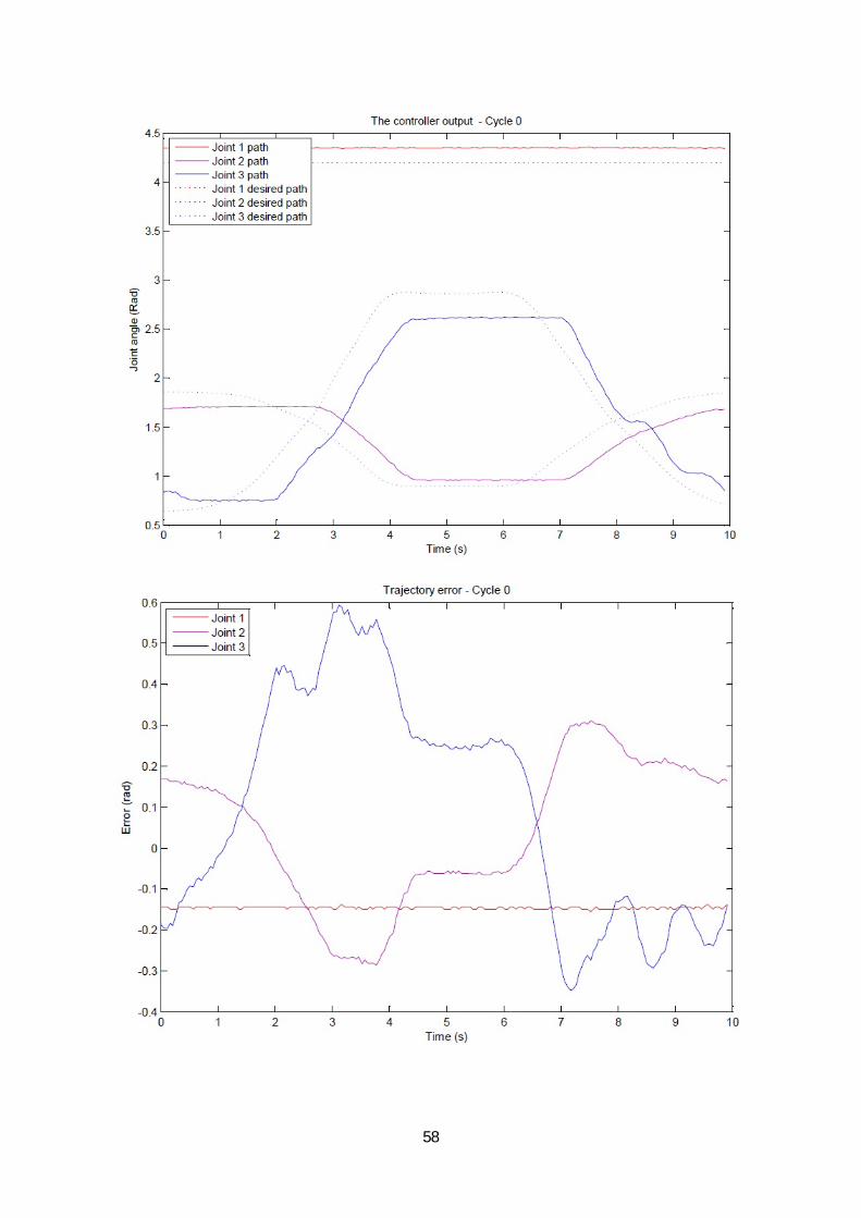
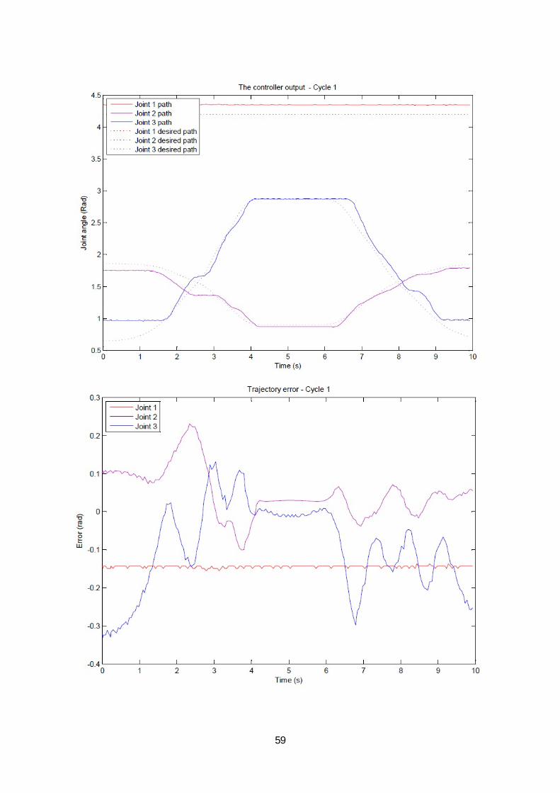
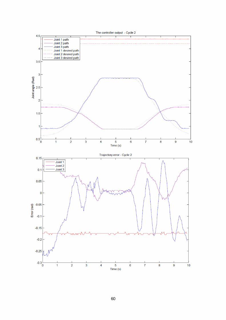
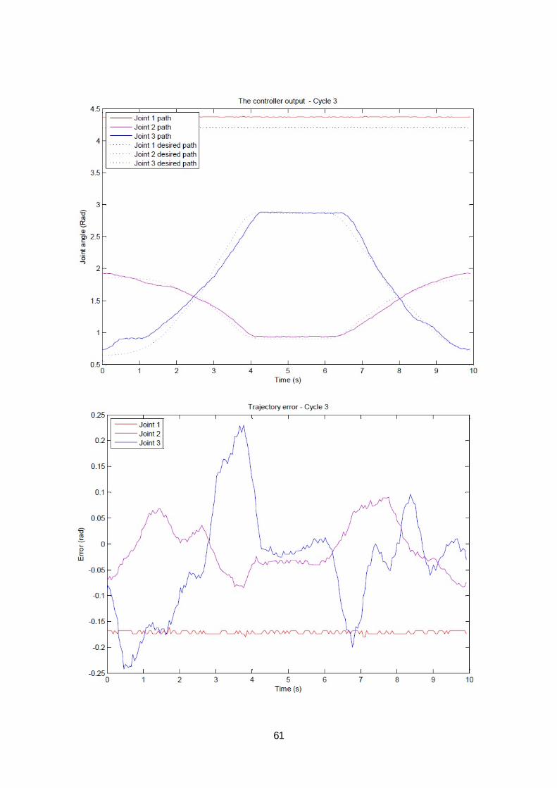
figure 6.9. As it is shown in the figures at cycle 0 that the controller performs without help of

ANN the error is relatively high. The error of the controller is decreased from cycle 0 to cycle

12 of training but after that as it is illustrated in last two figures the performance reduces

because of over fitting the network. Over fitting happens because the network is provided

with noisy data. To avoid over fitting another code is needed to check the performance of the

controller and stop the training if the performance drops during some consecutive cycles.

Then the weights are updated with the last successful performance of the controller.

A good point in training the network is that as long as the ANN is trained the error in the

system is reduced and the ideal signal that is required to be applied to motors, such that the

robot moves through desired path without error, is more constructed. With reduction in the

error the output of the PID reduces and the construction of signal is slowed down. In order to

increase the convergence of error, one possible way is to increase the gain values of the PID

controller. However it increases the risk of system instability.

46

47

48

49

Figure 6.9 Response to two point path - joint feedback and joint control

50

6.3.4 Joint control with Cartesian feedback

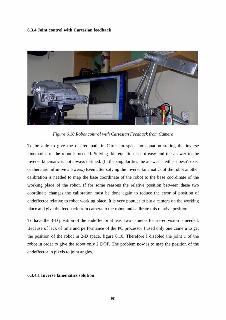
Figure 6.10 Robot control with Cartesian Feedback from Camera

To be able to give the desired path in Cartesian space an equation stating the inverse

kinematics of the robot is needed. Solving this equation is not easy and the answer to the

inverse kinematic is not always defined. (In the singularities the answer is either doesn't exist

or there are infinitive answers.) Even after solving the inverse kinematics of the robot another

calibration is needed to map the base coordinate of the robot to the base coordinate of the

working place of the robot. If for some reasons the relative position between these two

coordinate changes the calibration must be done again to reduce the error of position of

endeffector relative to robot working place. It is very popular to put a camera on the working

place and give the feedback from camera to the robot and calibrate this relative position.

To have the 3-D position of the endeffector at least two cameras for stereo vision is needed.

Because of lack of time and performance of the PC processor I used only one camera to get

the position of the robot in 2-D space, figure 6.10. Therefore I disabled the joint 1 of the

robot in order to give the robot only 2 DOF. The problem now is to map the position of the

endeffector in pixels to joint angles.

6.3.4.1 Inverse kinematics solution

51

To solve the inverse kinematic problem another ANN is implemented. As mentioned before

the ANNs are powerful for solving nonlinear systems and since they can learn the parameters

of the system the mapping does not need calibration. The network structure for this task is

similar to controller structure, figure 4.3. The only difference is that this network as two

inputs and two outputs.

The training procedure is that fist I trained the network with data from the camera and

position of the robot and then used the network to solve the inverse kinematic problem which

means by giving a path in camera pixels the robot should be able to find the correlated joint

angles and follows the path.

The procedure of collecting the training data is that a pixel in camera correlates to a vector in

joint space. Training the network is done such that the robot moves randomly and in every

time step the position of the endeffector in pixels and angle of joints in radians are recorded

as pair of input and output of the Neural Network. The network then is trained with this data

to solve the inverse kinematic problem. To train the network with data close to desired path it

is possible to put the robot manually in some points on the desired path and use those

positions as the training samples and increase the accuracy of the network output. The

kinematics mapping that come out from this procedure is strongly related to the robot-camera

relative positions and to the camera lens distortion.

6.3.4.2 Control method

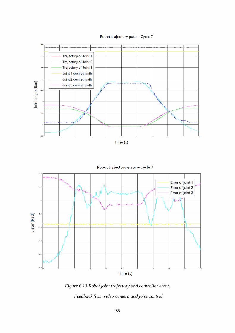
Figure 6.11 shows the structure of this controller. After training the ANN2, with a change in

the structure of the controller, now it is possible to give the path of robot in Cartesian space.

The trajectory path of the controller in joint space and the error of the controller are

illustrated in figure 6.13. As the cycles of training increases, the performance of the controller

increases as well but unfortunately the accuracy of the ANN to map endeffector position from

pictures to joint space was not enough, and the position of endeffector did not lie within

satisfactory range in the Cartesian space. The reasons for this low performance might be

- Distortion in the focal lens of the camera

- Error in reading endeffector position from camera and image processing

- Error in reading joints position from encoders due to noise and mechanic backlash

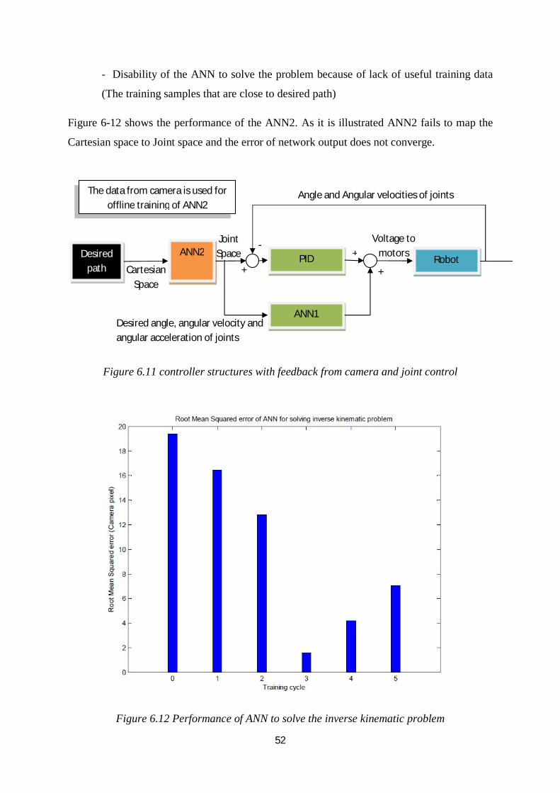
52

- Disability of the ANN to solve the problem because of lack of useful training data

(The training samples that are close to desired path)

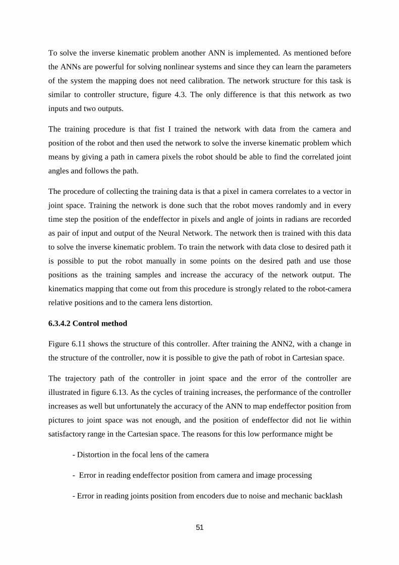
Figure 6-12 shows the performance of the ANN2. As it is illustrated ANN2 fails to map the

Cartesian space to Joint space and the error of network output does not converge.

Figure 6.11 controller structures with feedback from camera and joint control

Figure 6.12 Performance of ANN to solve the inverse kinematic problem

Robot PID Controller

ANN1

ANN2 Desired path Cartesian

Space

Joint Space

Voltage to motors

+

+

+

-

Angle and Angular velocities of joints The data from camera is used for offline training of ANN2

Desired angle, angular velocity and angular acceleration of joints

53

54

55

Figure 6.13 Robot joint trajectory and controller error,

Feedback from video camera and joint control

56

6.3.5 Cartesian control with Cartesian feedback

In order to avoid the error of ANN2 in the previous controller I changed the structure of

controller and ANN1 such that the ANN1 receives input directly from camera in camera

pixels and generates the proper control signal. By doing this the Artificial Neural Network

Controller (ANNC) is not required to solve the inverse kinematic problem and the inverse

kinematic problem is somehow handled by the ANNC itself.

6.3.6 Control method

Controller structure is shown in figure 6.14. As it is shown there are two ANNs is the

controller structure. ANN1 gets the desired path from Cartesian space and generates the

control signal. To train ANN1, in every robot cycle the motion of robot is recorded with the

camera and after that in offline mode this recorded movie is processed and the position of the

endeffector is driven and is stored in a vector. Afterward the acceleration and velocity of the

endeffector in Cartesian space are calculated by differentiating from the position vector with

respect to time. This [position, velocity, acceleration] vector is used as the training data to the

ANN1. To complete the training data pairs (network inputs and output) the output of the

controller is needed. Since the controller output is logged to a variable during robot operation

with time stamps, now the problem is to calculate the controller output at the time that the

image was captured. It is easily done by interpolating the controller output at the time that the

image was captured. The vector [position, velocity acceleration, torque] is used to train the

ANN and improve its performance for the next cycle of robot operation.

The ANN2 is required to calculate the inverse kinematics of the system and provide the

desired path to the PID controller in joint angles. The procedure of training ANN2 is same as

last section and it is very important that the error of inverse kinematic solution be close to

zero. The reason is that if there be an error in the inverse kinematic solution there are two set

points in the system and PID controller tries to move the robot to a wrong position. In this

case the ANN1 and the PID are competing against each other to move the robot to their set

points which are slightly different from each other.

A solution to this problem is to reduce the error of ANN2 output as much as possible and

decrees the PID gains as the training of the ANN1 continues. But this reduction of the gain

will decrease the robustness of the system and there should be a balance between the PID

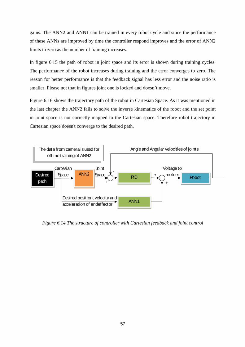
57

gains. The ANN2 and ANN1 can be trained in every robot cycle and since the performance

of these ANNs are improved by time the controller respond improves and the error of ANN2

limits to zero as the number of training increases.

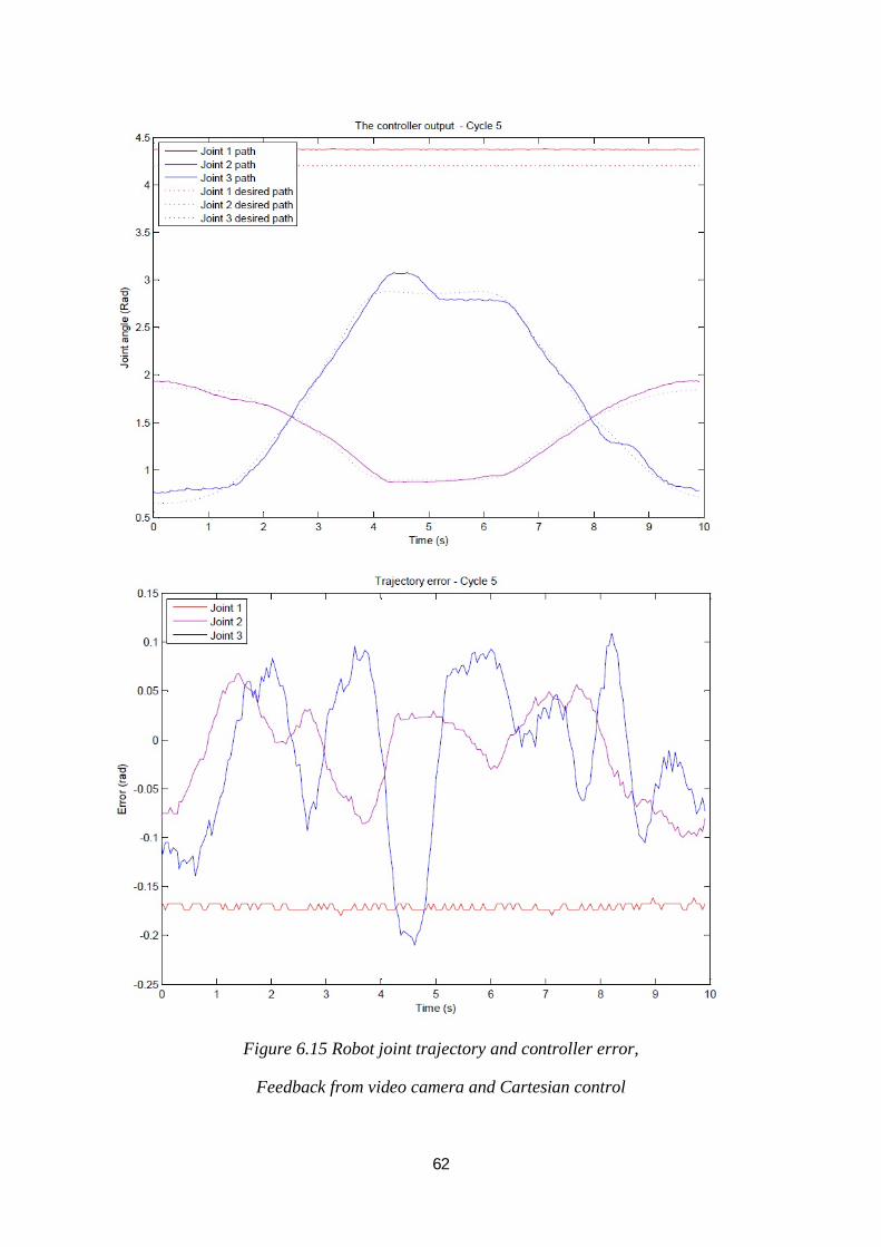
In figure 6.15 the path of robot in joint space and its error is shown during training cycles.

The performance of the robot increases during training and the error converges to zero. The

reason for better performance is that the feedback signal has less error and the noise ratio is

smaller. Please not that in figures joint one is locked and doesn’t move.

Figure 6.16 shows the trajectory path of the robot in Cartesian Space. As it was mentioned in

the last chapter the ANN2 fails to solve the inverse kinematics of the robot and the set point

in joint space is not correctly mapped to the Cartesian space. Therefore robot trajectory in

Cartesian space doesn't converge to the desired path.

Figure 6.14 The structure of controller with Cartesian feedback and joint control

Robot PID Controller

ANN1

ANN2 Desired path

Cartesian Space

Joint Space

Voltage to motors

+

+

+

-

Angle and Angular velocities of joints

Desired position, velocity and acceleration of endeffector

The data from camera is used for offline training of ANN2

58

59

60

61

62

Figure 6.15 Robot joint trajectory and controller error,

Feedback from video camera and Cartesian control

63

7 Conclusions

In this thesis an efficient method for control of a manipulator with arbitrary degrees of

freedom introduced. The ANN is used to identify both the dynamics and the kinematics of a

manipulator. Two different applications have been set up and described in the thesis.

Although this controller is not performing well during the first cycles of a new path but its

performance converges to zero during repetitive performance of robot. The controller design

is independent from parameters of the system and controller learns the system parameters

during its operation. The other advantage is that since the calculations are in parallel it is

possible to design the controller on an FPGA board with lower price and faster performance.

At the end the controller performance is tested by the simulation and in reality using

MATLAB robotic toolbox and a 3DOF robotic manipulator.

8 Future works

The topic of the thesis is related to other fields in robotics and there are lots of jobs than can

be done in future. One good idea is to use Dynamic networks with concurrent layers and

dynamic structures instead of a feed forwarded network because a network with this structure

can solve more complex systems and the controller may show better performance in practice.

The other good idea is to somehow increase the robustness of controller by changing the

structure of the network such that the ANN controller receives feedback from the manipulator

as a separate input. It is also possible to feed time to the network and analyze the performance

of the controller to time varying systems.

As it was shown in the results the robot performs better when it gets feedback from the

Cartesian space and it is a good idea to solve the inverse kinematics of the robot in 3

dimensions with combining stereo vision and the Artificial Neural Networks. The other task

that can increase the performance of the robot is to use a real-time operation system to control

the robot or implement the ANN on an FPGA board for online processing

At last since the network can learn the structure of the manipulator using this controller on a

robot with flexible links may lead to interesting results.

64

9 References

1. Proceedings of I993 International Joint Conference on Neural Networks, ROBOTIC

MANIPULAI'OR TRAJECTORY CONTROL USING NEURALNETWORKS Bin Jin

Department of Electrical Engineering, Shanghai University of Technology, 149 Yan-chang

Road, Shanghai 200072, P.R. Chinam.

2. Trajectory Control of Robotic Manipulators Using Neural Networks, Tomochika

Ozaki, Tatsuya Suzuki, Member, IEEE, Takeshi Furuhashi, Member, IEEE, Shigeru Okuma,

Member, IEEE, and Yoshiki Uchikawa.

3. Adaptive Neural Network Control of Robot Manipulators in Task Space, Shuzhi S.

Ge, Member, IEEE, C. C. Hang, Senior Member, IEEE, and L. C. Woon.

4. A Neural Network for the Trajectory Control of Robotic Manipulators with

Uncertainties, Boo Hee Nam, Sang Jae Lee, and Seok Won Lee, ERC-ACI, Dept. of Control

and Instrumentation Eng., Kangwon National Univ., Chunchon, Kangwondo 200-701, Korea

5. A new neural network control technique for robot manipulators, seul jung and T.C.

Hsia, Robotics Research Laboratory, Department of Electrical and computer Engineering,

University of California.

6. Possibility of Neural Networks Controller for Robot Manipulators' Tetsuro YABUTA

and Takayuki YAMADA NTT Transmission Systems Laboratories, Tokai, Ibaraki, 31 9-1 1,

JAPAN.

7. A Neural Network Control of Robot Manipulators and Nonlinear Systems AvFrank L.

Lewis, Suresh Jagannathan,

8. Robotics Dynamics and Control by Mark W.Spong amd M.Vidyasagar.

65

9. Comparative Study of Neural Network Structures in Identification of Non-linear

Systems M. Önder Efe and Okyay Kaynak Mechatronics Research and Application Center,

Bogaziçi University, Bebek, 80815 Istanbul.

10. A Neural Network Compensator for Uncertainties of Robotics Manipulators Akio

Ishiguro, Takeshi Furuhashi, Shigeru Okuma, Member, ZEEE, and Yoshiki Uchikawa.

11. Matlab robotics toolbox by peter I.Corke. http://www.ict.csiro.au/downloads/robotics/

12. A Method for the Solution of Certain Non-Linear Problems in Least Squares, Kenneth

Levenberg (1944). The Quarterly of Applied Mathematics 2: 164–168.

13. Matlab help for trainlm, http://www.math.muni.cz/matlab/toolbox/nnet/trainlm.html

14. http://www.adinco.nl/site/media/downloads/aandrijftechniek/A88 RH158 DC-motor

with integrated gearbox rev1.pdf

15. H-bridge with power MosFet, http://www.armory.com/~rstevew/Public/Motors/H-

Bridges/Blanchard/h-bridge.htm

16. Help for Matlab real-time windows target. http://www.mathworks.com/products/rtwt/

17. Matlab help about wden denoise function.

http://matlab.izmiran.ru/help/toolbox/wavelet/wden.html