DESIGN AND SIMULATION OF FUZZY LOGIC CONTROL SYSTEM FOR

ROBOTIC TWO-LINK MANIPULATORS

Mr. N. Selvaganesan, Mr. Prabhu Jude. R, Dr. S.Renganathan, Mr. S.Magesh

Department of Instrumentation, Madras Institute of Technology, Chennai – 600 044.

ABSTRACT

Robotic manipulators are subjected to both structured and unstructured uncertainties even in a well-

structured setting. This paper attempts to design a fuzzy logic controller for controlling the position of the

arms of a two-link manipulators taking into account the disturbances caused by inertial loading, coupling

reaction forces between joints (Coriolis and centrifugal), and gravity loading effects. The design for the

position control incorporates a torque computation block that compensates for the disturbances caused by

these effects and a fuzzy logic controller. The simulation results for the position control of a two-link

robotic manipulator using the compensated fuzzy logic model were then compared with the results obtained

using an optimized PID controller. The results clearly indicated that the performance of the compensated

fuzzy logic controller was much better than the optimized PID controller even for nonlinear disturbances.

DESIGN AND SIMULATION OF FUZZY LOGIC CONTROL SYSTEM FOR ROBOTIC

TWO-LINK MANIPULATORS

Mr. N. Selvaganesan, Mr. Prabhu Jude. R, Dr. S.Renganathan, Mr. S.Magesh

Department of Instrumentation, Madras Institute of Technology, Chennai – 600 044.

1. Introduction

The robotic manipulators are highly coupled, nonlinear and time-varying systems that are generally subjected to

both structured and unstructured uncertainties. This makes the accurate position control of the robotic arms a

very complicated and difficult engineering problem. With the use of the robots in the medical and sensitive

industrial applications gaining popularity, the precision position control of the robot arms has turned into an

inevitable requirement. This demand for the accurate position control calls for a method that compensates by

and large for the adverse effects of the uncertainties on the positioning of the robot arms. The inertia, gravity

and Coriolis Effect have been identified as the major contributors for the inaccuracy in the positioning of the

robot arms. Hence an accurate controller invariably has to overcome these adverse effects by including some

kind of compensation logic in the design.

2. Robot Dynamics

Robot dynamics basically deals with mathematical formulations of the equations of robot arm motion. The

dynamic equations of motion of a manipulator are a set of mathematical equations describing the dynamic

behavior of the manipulator. Such equations of motion are useful for computer simulation of the robot arm

motion, design of suitable control equations of a robot arm and evaluation of kinematic design and structure of a

robot arm. The actual dynamic model can be obtained from known physical laws such as the laws of Newtonian

and Lagrangian mechanics.

3. L-E Formulation

The general motion equations of a manipulator can conveniently be expressed through the direct application of

the Lagrange Euler (L-E) formulation to non - conservative systems. The L-E equation is given as follows

d / dt (∂L / ∂qi’) - ∂L / ∂qi = τi i = 1,2,3,………n

where

L = Lagrangian function = kinetic energy K- potential energy P

K = total kinetic energy of the robot arm

P = total potential energy of the robot arm

qi = generalized coordinates of the robot arm

qi’= first time derivative of the generalized coordinate, qi

τi = generalized force (or torque) applied to the system at joint i to drive link i

From the above Lagrange-Euler equation, one is required to properly choose a set of generalized coordinates to

describe the system. Generalized coordinates are used as a convenient set of coordinates that completely

describe the location (position and orientation) of a system with respect to a reference coordinate frame. For a

simple manipulator with rotary-prismatic joints, various sets of generalized positions of the joints are readily

available because they can be measured by potentiometers or encoders or other sensing devices, they provide a

natural correspondence with the generalized coordinates. Thus, in the case of a rotary joint, qi ≡ θi, the joint

angle span of the joint.

4. Motion Equations of a manipulator

The derivation of equations of motion of a manipulator requires the computation of the total kinetic energy and

the total potential energy of the manipulator.

4.1 Kinetic Energy of the manipulator

If dKi is the kinetic energy of a particle with differential mass dm in link i; then

dKi = ½(xi2’ + yi

2’ + zi2’) dm

= ½ trace (vi viT) dm

=½ Tr (vi viT) dm

where vi = ( ∑j Ui j qj’ ) iri j varies from 1 to i

Ui j = 0 A j-1 Q j j-1A i for j <= i

0 for j > i

Qj is a 4 x 4 matrix, given as [ (0 –1 0 0), (1 0 0 0), (0 0 0 0), (0 0 0 0)] for revolute joint. …(1)

iri = fixed point at rest in a link ‘i’ w.r.t homogeneous coordinates of the ith link coordinate

i A j = homogeneous coordinate transformation matrix which relates jth coordinate frame to the ith

coordinate frame.

The total kinetic energy of all the links can be found out by integrating dKi over all the links.

The total kinetic energy K of a robot arm after integration will be found as

K = ∫ dKi = ½ Tr [ ∑p ∑r Uip ( Ji ) UirT qp’ qr’) ] p, r varies from 1 to i ……(2)

where

Ji is the inertia of all the points on link i given by

Ji = ∫ iri iri

T dm

4.2 Potential Energy of the Manipulator

Let Pi be the ith link’s potential energy. The Pi is given by

Pi = -mi g (0Ai i ři ) i = 1, 2, ……….. n

where 0Ai is the coordinate transformation matrix which relates the ith coordinate frame to the base coordination

frame

i ři is the a fixed point in the ith link expressed in homogenous coordinates with respect to the ith link

coordinate frame .

The total potential energy P of the robot manipulator is found out by integrating Pi over all the links.

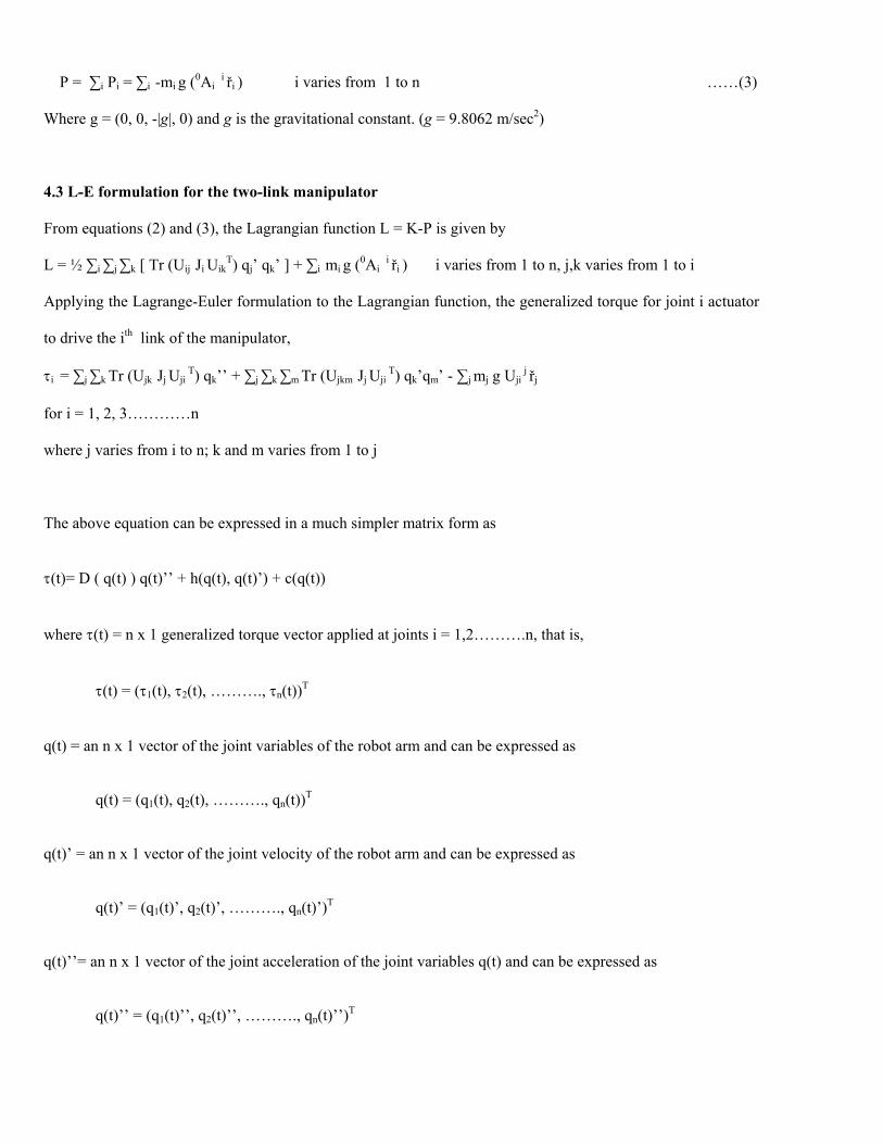
P = ∑i Pi = ∑i -mi g (0Ai i ři ) i varies from 1 to n ……(3)

Where g = (0, 0, -|g|, 0) and g is the gravitational constant. (g = 9.8062 m/sec2)

4.3 L-E formulation for the two-link manipulator

From equations (2) and (3), the Lagrangian function L = K-P is given by

L = ½ ∑i ∑j ∑k [ Tr (Uij Ji UikT) qj’ qk’ ] + ∑i mi g (0Ai i ři ) i varies from 1 to n, j,k varies from 1 to i

Applying the Lagrange-Euler formulation to the Lagrangian function, the generalized torque for joint i actuator

to drive the ith link of the manipulator,

τi = ∑j ∑k Tr (Ujk Jj Uji T) qk’’ + ∑j ∑k ∑m Tr (Ujkm Jj Uji

T) qk’qm’ - ∑j mj g Uji j řj

for i = 1, 2, 3…………n

where j varies from i to n; k and m varies from 1 to j

The above equation can be expressed in a much simpler matrix form as

τ(t)= D ( q(t) ) q(t)’’ + h(q(t), q(t)’) + c(q(t))

where τ(t) = n x 1 generalized torque vector applied at joints i = 1,2……….n, that is,

τ(t) = (τ1(t), τ2(t), ………., τn(t))T

q(t) = an n x 1 vector of the joint variables of the robot arm and can be expressed as

q(t) = (q1(t), q2(t), ………., qn(t))T

q(t)’ = an n x 1 vector of the joint velocity of the robot arm and can be expressed as

q(t)’ = (q1(t)’, q2(t)’, ………., qn(t)’)T

q(t)’’= an n x 1 vector of the joint acceleration of the joint variables q(t) and can be expressed as

q(t)’’ = (q1(t)’’, q2(t)’’, ………., qn(t)’’)T

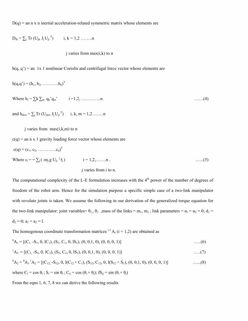
D(q) = an n x n inertial acceleration-related symmetric matrix whose elements are

Dik = ∑j Tr (Ujk Jj Uji T) i, k = 1,2 ……..n

j varies from max(i,k) to n

h(q, q’) = an 1x 1 nonlinear Coriolis and centrifugal force vector whose elements are

h(q,q’) = (h1, h2, ………..hn)T

Where hi = ∑k ∑m qk’qm’ i =1,2, ………….n. ……(4)

and hikm = ∑j Tr (Ujkm Jj Uji T) i, k, m = 1,2……..n

j varies from max(i,k,m) to n

c(q) = an n x 1 gravity loading force vector whose elements are

c(q) = (c1, c2, …………cn)T

Where ci = = ∑j ( -mj g Uji j řj ) i = 1,2,…….n . …...(5)

j varies from i to n.

The computational complexity of the L-E formulation increases with the 4th power of the number of degrees of

freedom of the robot arm. Hence for the simulation purpose a specific simple case of a two-link manipulator

with revolute joints is taken. We assume the following in our derivation of the generalized torque equation for

the two-link manipulator: joint variables= θ1,, θ2 ,mass of the links = m1, m2 , link parameters = α1 = α2 = 0; d1 =

d2 = 0; a1 = a2 = l.

The homogenous coordinate transformation matrices i-1 Ai (i = 1,2) are obtained as

0A1 = [(C1, -S1, 0, lC1), (S1, C1, 0, lS1), (0, 0,1, 0), (0, 0, 0, 1)] …..(6)

1A2 = [(C2, -S2, 0, lC2), (S2, C2, 0, lS2), (0, 0,1, 0), (0, 0, 0, 1)] …..(7)

0A2 = 0A1 1A2 = [(C12, -S12, 0, l(C12 + C1), (S12, C12, 0, l(S12 + S1), (0, 0,1, 0), (0, 0, 0, 1)] …...(8)

where Ci = cos θi ; Si = sin θi ; Cij = cos (θi + θj); fSij = sin (θi + θj)

From the eqns 1, 6, 7, 8 we can derive the following results

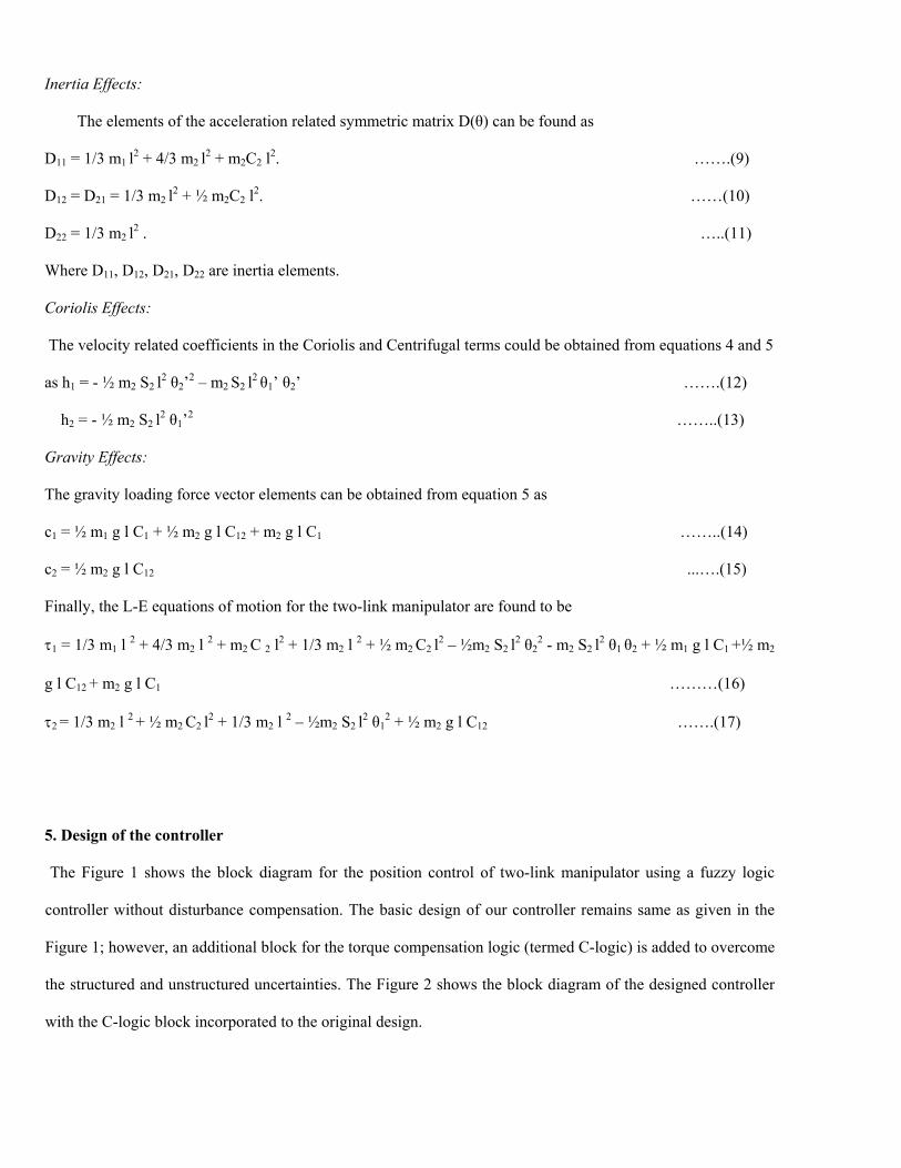
Inertia Effects:

The elements of the acceleration related symmetric matrix D(θ) can be found as

D11 = 1/3 m1 l2 + 4/3 m2 l2 + m2C2 l2. …….(9)

D12 = D21 = 1/3 m2 l2 + ½ m2C2 l2. ……(10)

D22 = 1/3 m2 l2 . …..(11)

Where D11, D12, D21, D22 are inertia elements.

Coriolis Effects:

The velocity related coefficients in the Coriolis and Centrifugal terms could be obtained from equations 4 and 5

as h1 = - ½ m2 S2 l2 θ2’2 – m2 S2 l2 θ1’ θ2’ …….(12)

h2 = - ½ m2 S2 l2 θ1’2 ……..(13)

Gravity Effects:

The gravity loading force vector elements can be obtained from equation 5 as

c1 = ½ m1 g l C1 + ½ m2 g l C12 + m2 g l C1 ……..(14)

c2 = ½ m2 g l C12 ...….(15)

Finally, the L-E equations of motion for the two-link manipulator are found to be

τ1 = 1/3 m1 l 2 + 4/3 m2 l 2 + m2 C 2 l2 + 1/3 m2 l 2 + ½ m2 C2 l2 – ½m2 S2 l2 θ22 - m2 S2 l2 θ1 θ2 + ½ m1 g l C1 +½ m2

g l C12 + m2 g l C1 ………(16)

τ2 = 1/3 m2 l 2 + ½ m2 C2 l2 + 1/3 m2 l 2 – ½m2 S2 l2 θ12 + ½ m2 g l C12 …….(17)

5. Design of the controller

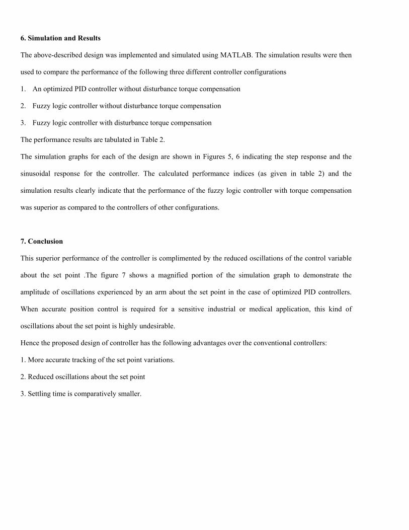
The Figure 1 shows the block diagram for the position control of two-link manipulator using a fuzzy logic

controller without disturbance compensation. The basic design of our controller remains same as given in the

Figure 1; however, an additional block for the torque compensation logic (termed C-logic) is added to overcome

the structured and unstructured uncertainties. The Figure 2 shows the block diagram of the designed controller

with the C-logic block incorporated to the original design.

The design of the individual blocks is summarized below.

5.1 C-Logic Block

The C-Logic block shown here can be expressed as a combination of the L-E torque computation block and a

torque to voltage converter (T-V converter). The C-Logic block can be delineated as shown in Figure 3. The

torque computation block calculates the torque experienced in the joints 1 and 2 from the generalized angular

coordinate position of the arms as given by the equations 16 and 17 .The torque outputs are then fed to the T-V

converter .The T-V converter calculates the voltage that corresponds to a particular combination of torque (τ)

and the time derivative of the angular position of the arm (θ) as given by the formula

v = [θ’ Kfb + (τ * R m) / Ktorque ] * Gear Ratio

where Kfb=feed back constant

Ktorque=torque constant

Rm= mechanical resistance

5.2 Fuzzy Logic Controller

In our case we designed a fuzzy controller with the error and the first derivative of the error as fuzzy inputs .The

error is calculated as the difference between the set point of the arm position and the instantaneous position of

the arm. We used the triangular membership function for the fuzzification of the input variables. A 7x7 rule

base was designed for each of the two controllers. The output from the inference engine is defuzzified using the

center of area methods of defuzzification.

5.3 Robot Dynamics Block

This block uses the mechanical and electrical characteristics of the manipulator to convert the voltage input into

an equivalent angular position output. The Figure 4 represents the robot dynamics model that we used in our

simulation.

6. Simulation and Results

The above-described design was implemented and simulated using MATLAB. The simulation results were then

used to compare the performance of the following three different controller configurations

1. An optimized PID controller without disturbance torque compensation

2. Fuzzy logic controller without disturbance torque compensation

3. Fuzzy logic controller with disturbance torque compensation

The performance results are tabulated in Table 2.

The simulation graphs for each of the design are shown in Figures 5, 6 indicating the step response and the

sinusoidal response for the controller. The calculated performance indices (as given in table 2) and the

simulation results clearly indicate that the performance of the fuzzy logic controller with torque compensation

was superior as compared to the controllers of other configurations.

7. Conclusion

This superior performance of the controller is complimented by the reduced oscillations of the control variable

about the set point .The figure 7 shows a magnified portion of the simulation graph to demonstrate the

amplitude of oscillations experienced by an arm about the set point in the case of optimized PID controllers.

When accurate position control is required for a sensitive industrial or medical application, this kind of

oscillations about the set point is highly undesirable.

Hence the proposed design of controller has the following advantages over the conventional controllers:

1. More accurate tracking of the set point variations.

2. Reduced oscillations about the set point

3. Settling time is comparatively smaller.

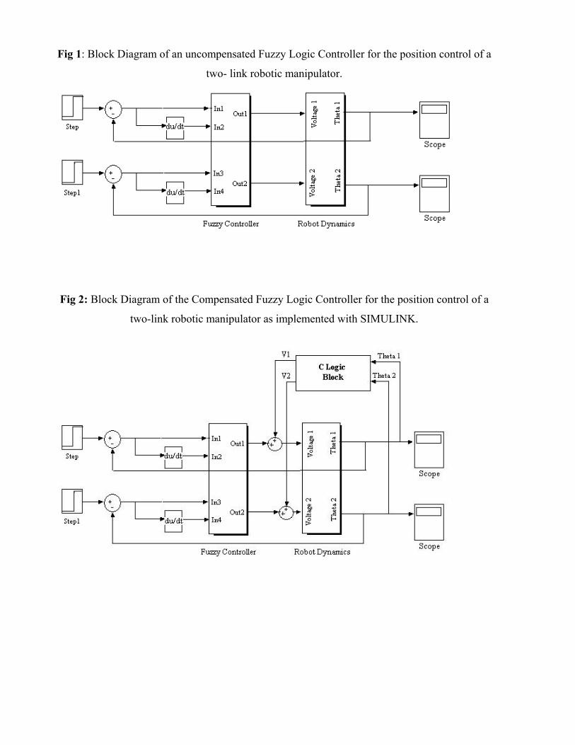
Fig 1: Block Diagram of an uncompensated Fuzzy Logic Controller for the position control of a

two- link robotic manipulator.

Fig 2: Block Diagram of the Compensated Fuzzy Logic Controller for the position control of a

two-link robotic manipulator as implemented with SIMULINK.

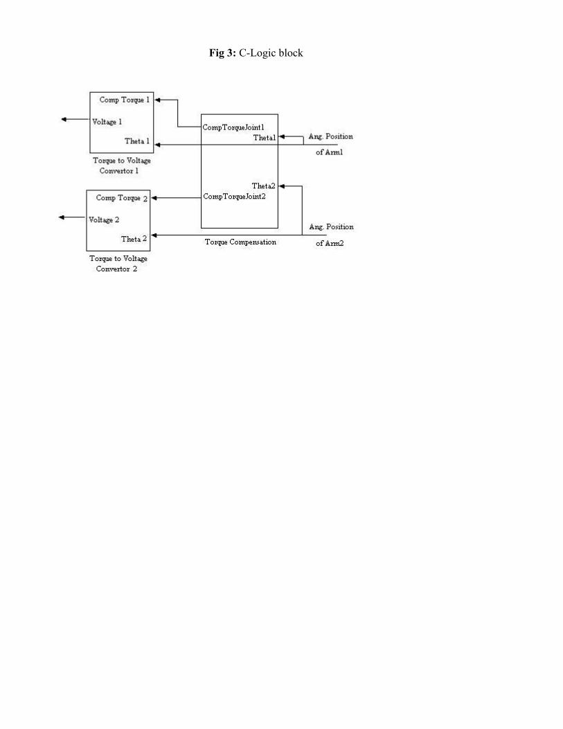
Fig 3: C-Logic block

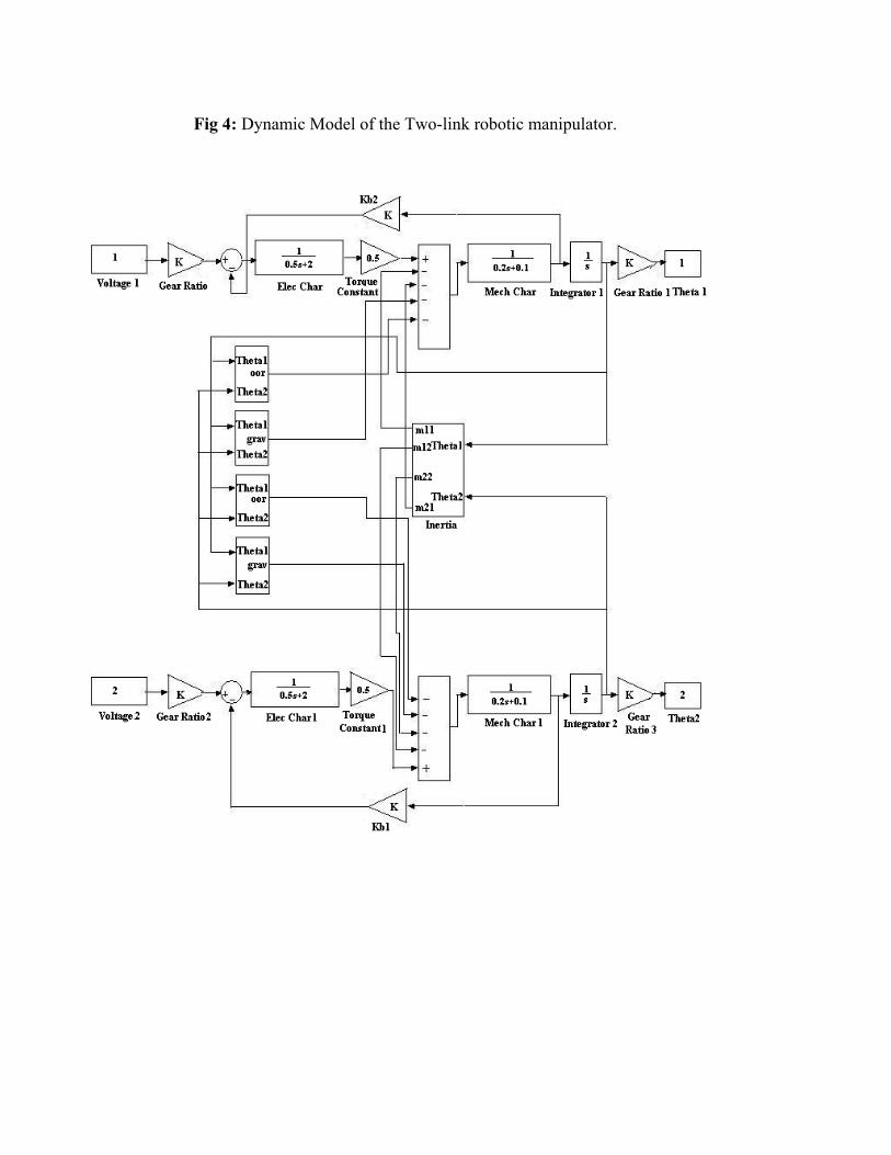
Fig 4: Dynamic Model of the Two-link robotic manipulator.

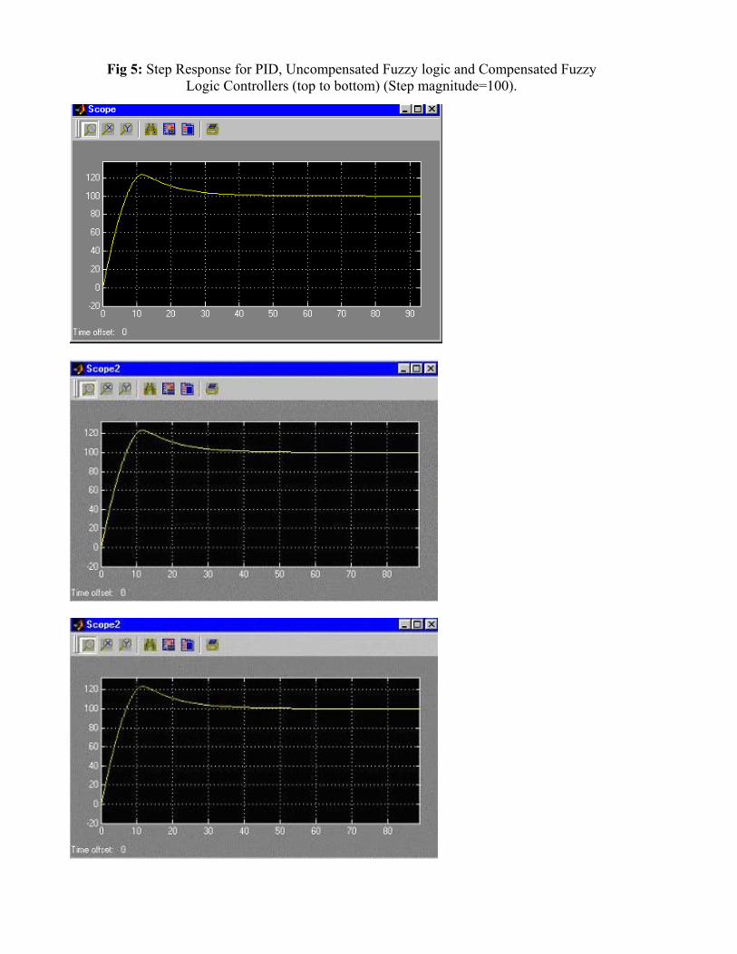
Fig 5: Step Response for PID, Uncompensated Fuzzy logic and Compensated Fuzzy Logic Controllers (top to bottom) (Step magnitude=100).

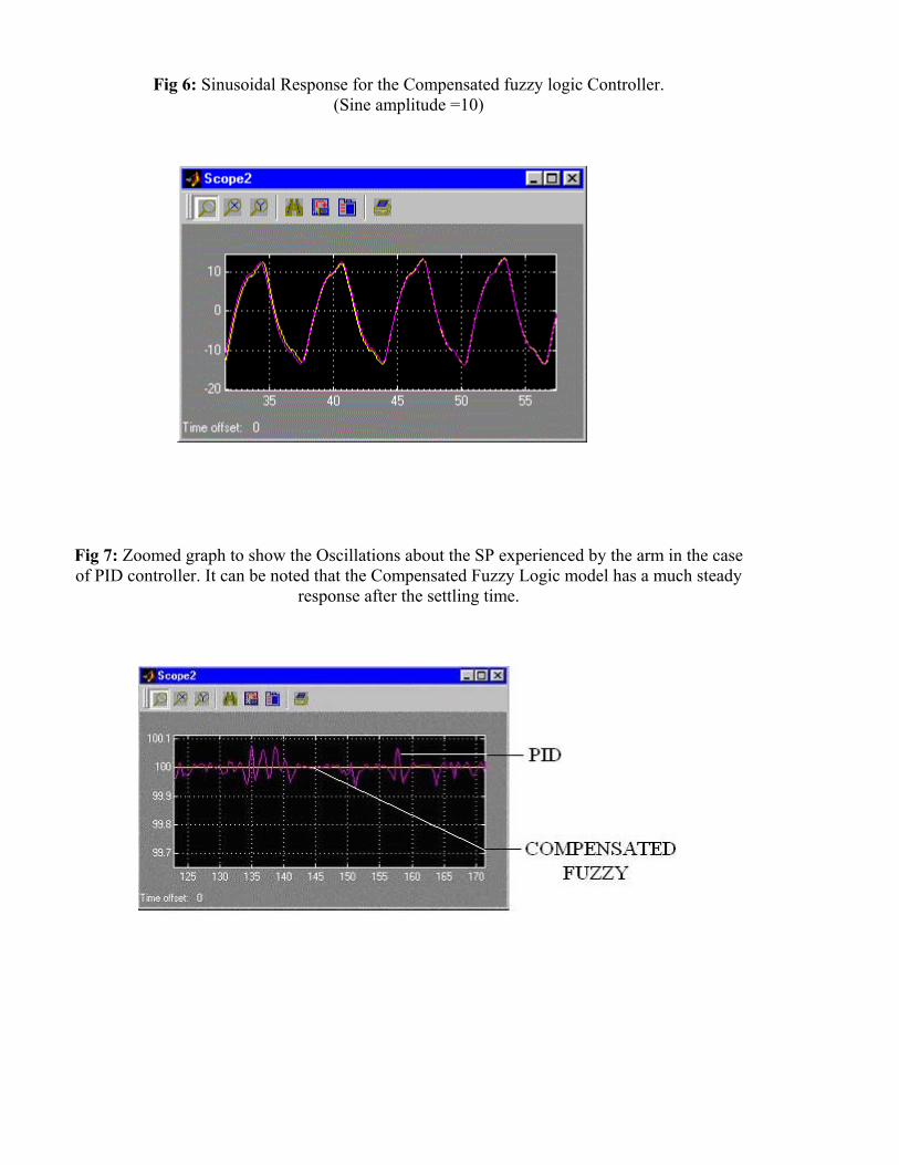
Fig 6: Sinusoidal Response for the Compensated fuzzy logic Controller. (Sine amplitude =10)

Fig 7: Zoomed graph to show the Oscillations about the SP experienced by the arm in the case of PID controller. It can be noted that the Compensated Fuzzy Logic model has a much steady

response after the settling time.

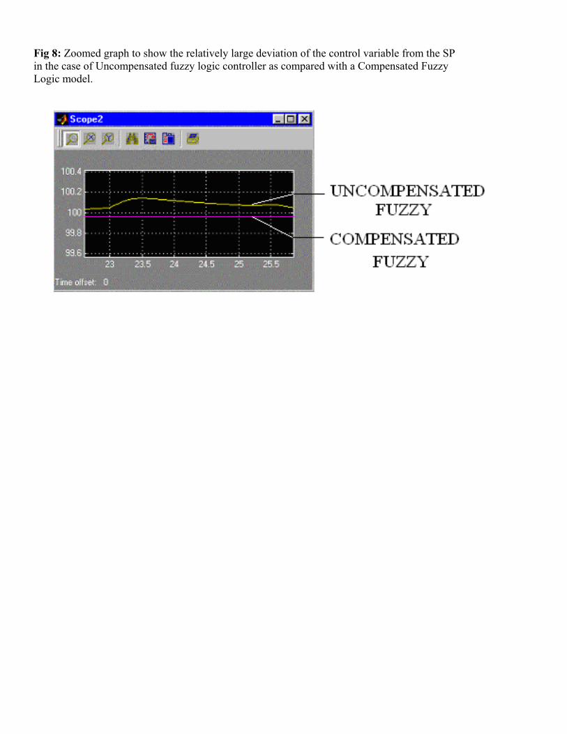
Fig 8: Zoomed graph to show the relatively large deviation of the control variable from the SP in the case of Uncompensated fuzzy logic controller as compared with a Compensated Fuzzy Logic model.

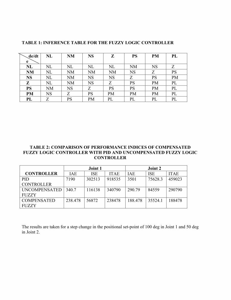
TABLE 1: INFERENCE TABLE FOR THE FUZZY LOGIC CONTROLLER

de/dt e

NL NM NS Z PS PM PL

NL NL NL NL NL NM NS Z NM NL NM NM NM NS Z PS NS NL NM NS NS Z PS PM Z NL NM NS Z PS PM PL PS NM NS Z PS PS PM PL PM NS Z PS PM PM PM PL PL Z PS PM PL PL PL PL

TABLE 2: COMPARISON OF PERFORMANCE INDICES OF COMPENSATED FUZZY LOGIC CONTROLLER WITH PID AND UNCOMPENSATED FUZZY LOGIC

CONTROLLER

Joint 1 Joint 2 CONTROLLER IAE ISE ITAE IAE ISE ITAE PID CONTROLLER

7190 302513 918535 3501 75628.3 459023

UNCOMPENSATED FUZZY

340.7 116138 340790 290.79 84559 290790

COMPENSATED FUZZY

238.478 56872 238478 188.478 35524.1 188478

The results are taken for a step change in the positional set-point of 100 deg in Joint 1 and 50 deg in Joint 2.

REFERENCES:

1. R. R. Yager, D. P. Filev, “Essentials of Fuzzy Modeling and Control”, New York:

Wiley (1994)

2. S. Commuri, F. L.Lewis, “Adaptive-Fuzzy Controllers of Robot manipulators”, Int.

J. Syst. Sci., vol.27, no.6 (1996)

3. J. J. Craig, “Introduction to Robotics”, New York: Addison Wesley (1989)

4. Limin Peng, Peng-Yung Woo, “Neural-Fuzzy Control System for Robotic

Manipulators”, IEEE Control System Magazine, vol.22, no.1 (2002)

5. K.S.Fu, R.C.Gonzalez, C.S.G.Lee, "Robotics-Control, Sensing, Vision and

Intelligence", McGraw Hill Book Company (1987).