fluid mechanics for gravity-flow water systems and pumps ...i) parallel pipes 15 ii) water sources...
TRANSCRIPT
1
Fluid Mechanics For Gravity-Flow
Water Systems and Pumps
Made Simple (?)
Issue 2 May 2003

2
Issue Changes
Issue Date Change
1 April 2001 -
2 May 2003 1. Preface and Notes added.
2. Glossary expanded.
3. References relocated.
4. Appendix 5 : Interpolation added.
5. Appendix 6 : Frictional Head Loss Chart added.
6. Worked Examples typed and revised.
3
Contents
Section Page
Glossary 4
Preface 5
References 5
Notes 5
1. Introduction 6
2. General Concepts 6
3. Derivation of the Continuity Equation 7
4. The Continuity Equation for Multiple Pipe Sections 8
5. Energy in a Perfect System : The Bernoulli Equation 8
6. Imperfect Systems : Friction and the Bernoulli Equation 9
7. Pumps and Turbines : The Bernoulli Equation 10
8. Typical Scenarios 11
i) Natural Flow 11
ii) Controlled Flow : Valves Open 12
iii) Controlled Flow : Valves Shut 12
iv) Pump Requirement 13
v) General Equation for Distribution Systems 14
9. Special Scenarios 15
i) Parallel Pipes 15
ii) Water Sources at Different Elevations 16
Appendix 1. Kinetic Energy of a Fluid 18
Appendix 2. Potential Energy of a Fluid 19
Appendix 3. Friction Losses and the Reynolds Number 20
Appendix 4. Water System Design Parameters 21
Appendix 5. Interpolation 22
Appendix 6. Frictional Head Loss Chart 24
Worked Examples 25
1. Natural flow 26
2. Natural flow with pipes of different diameters and lengths 27
3. Simple tap system (tap open) 29
4. Simple tap system (tap shut) 30
5. Pump requirement 30
6. Distribution systems : The general equation 32
7. Parallel pipes 34
8. Sources at different elevations 36
9. Sample water system design 38

4
Glossary
Term Description Units
a Acceleration Metres/Second 2
A Area Metres 2 At Reservoir Supply Pipe Area Metres 2 D,d Pipe Diameter Metres/inches E Energy Joules Ek Kinetic Energy Joules Ep Potential Energy Joules F Force Newtons f Friction Factor -
fA-n Frictional Head Loss in Tap Supply Pipe Metres fh Frictional Head Loss Metres fhl Frictional Head Loss in Larger Diameter Pipe Metres fhn Frictional Head Loss in Pipe n Metres fhs Frictional Head Loss in Smaller Diameter Pipe Metres fp Frictional Loss (Pressure) Newtons/Metre 2
ft-A Frictional Head Loss in Reservoir Supply Pipe Metres g Gravitational Acceleration Metres/Second 2 h Height Metres H Desired Frictional Head Loss Metres hA Height of Junction A Metres HA Head at Point A Metres hB Height of Junction B Metres
Hmax Maiximum Static Head Metres hn Height of nth Tap Metres Hn Residual Head at Tap n Metres ht Reservoir Height Metres I Electrical Current Amps L Length Metres Ln nth Tap Supply Pipe Length Metres Lt Reservoir Supply Pipe Length Metres M Mass Kilogrammes n Number of Taps -
NRE Reynolds Number - P Pressure Newtons/Metre 2 PA Pressure at Junction A Newtons/Metre 2 PB Pressure at Junction B Newtons/Metre 2 Pk Kinetic Energy as a Pressure Newtons/Metre 2 Pn Residual Pressure at nth tap Newtons/Metre 2 Pp Pump Pressure Newtons/Metre 2 Pp Potential Energy as a Pressure Newtons/Metre 2 Pt Turbine Pressure Newtons/Metre 2
Q,q Volumetric Flow Rate Metre 3/Second qA Volumetric Flow Rate at Junction A Metre 3/Second S Distance Metres t Time Seconds v Velocity Metres/second V Volume Metre 3 V Voltage Volts vA Velocity of Water in Reservoir Supply Pipe Metres/Second vav Average Velocity Metres/Second vn Velocity of Water in nth Tap Supply Pipe Metres/Second W Power Watts We Electrical Power Watts Win Power Supplied to Pump Watts Wout Power Supplied by Pump Watts
∆h Total Difference in Head between Tanks Metres
∆H Residual Head Metres
∆P Residual Pressure Newtons/Metre 2
γ Pump Efficiency -
µk Kinematic Viscosity Metres 2/Second
ρ Density (ro) Kilogrammes/Metre 3
5
Preface This manual is intended to aid the water projects worker or volunteer in the following ways :
1. To explain, from first principals and using basic physical relations, the origin of the equations that design water
systems.
2. To systematically outline the key equations and explain how to apply them to scenarios where there is no text
book method readily available.
3. To give step by step numerical solutions to some of the more common and also some special scenarios.
4. To systematically lay down the design parameters for gravity flow water systems and show how they should be
applied to a design.
Sections 2-7 explain the basic concepts, show how the core equations are derived, explain perfect and imperfect systems
and cover the analysis of pumps and turbines.
Sections 8 and 9 show how to apply the core equations to a series of common and special scenarios.
The worked examples 1-8 show how to simplify the equations developed in Sections 8 and 9 for practical use and give
step by step numerical examples for each scenario. In addition worked example 9 shows the design process applied to a
sample gravity flow water system design.
Appendices 1-6 give more complex derivations of the core relations, explanations of useful processes in the calculations
and additional technical data.
For the experienced water system designer I would suggest reading through Sections 8 and 9, Appendix 4 and Worked
Example 9 in particular.
Any questions about this manual should be addressed to Dodger at [email protected].
References
1. A Handbook of Gravity-Flow Water Systems : Thomas D.Jordan Jnr. : Intermediate Technology Publications 1996.
2. Basic Engineering Sciences and Structural Engineering for Engineer-in-Training Examinations : Apfelbaum &
Ottesen : Hayden Book Company 1970.
3. Friction Loss Characteristics Chart : Polyethylene (PE) SDR-Pressure Rated Tube : PISTA & Gustavo Urbano.
Notes 1. In the numerical calculations for the Worked Examples, the asterisk (*) denotes the multiplication sign and the slash
(/) the divide sign.
2. In general, metric fundamental units (Metres, Kilogrammes and Seconds) have been used in the Worked Examples,
the two main exceptions being inches for pipe diameters and Litres/Second (LPS) for flow rates.

6
1. Introduction
There are basically two equations needed to design gravity flow water systems :
1. The Continuity Equation
2. The Bernoulli Equation
With these two relations and an understanding of frictional effects most systems can be designed and/or analysed.
2. General Concepts
The following are the basic equations which can be used to derive the Continuity and Bernoulli Equations :
Relation Equation Units
(1) Velocity = Distance Moved/Time v = S/t Metres/Second (m/s)
Example : If I run 100 metres in 10 seconds (in a straight line), I have a velocity of 100/10 = 10 metres per second (m/s).
(2) Acceleration = Velocity Change/Time a = (v2 – v1)/t Metres/Second 2 (m/s
2)
Example : If at the start of the 100m race I have a velocity of zero (I am in the blocks) and after 2 seconds I have a
velocity of 10 m/s then my acceleration is (10-0)/2 = 5 metres per second per second (a = (v2 – v1)/t ). This means I
increase my velocity by 5 metres/second every second that passes. This is my average acceleration.
(3) Force = Mass.Acceleration F = M.a Kilogramme Metres/Second 2 (Kg.m/s
2) or Newtons (N)
Example : If I throw a bucket of water at you, you will feel a force when the water hits you because the water is
decelerating. Suppose the water had a mass of 10 Kg , was travelling at 5m/s before it hit you and took 1 second to slow
down. The deceleration of the water is 5/1 = 5 metres per second per second and so the force applied to you is 5 x 10 = 50
Newtons (F = M.a).
(4) Pressure = Force/Area P = F/A Newtons/Meter 2 (N/m
2) or Pascals (Pa)
Example : I wear my training shoes and step on your foot. If I then step on your foot wearing my stilettos, you will feel
the difference in pressure. This is because the force (my weight) is the same, but the area over which it is applied (the heel
of the stiletto) is smaller, so the pressure is higher. If I have a mass of 70 Kg, then my force due to gravity is 70 x 9.81 =
687 Newtons. If the area of my training shoe is 0.0075 m2 (75 cm
2) then the pressure due to it on your foot is 687/0.0075
= 91600 N/m2 or Pa. If the area of my stiletto heel is 0.0001 m
2 (1cm
2) then the pressure due to it on your foot is
687/0.0001 = 6870000 N/m2 or Pa. This is why it hurts !
(5) Density = Mass/Volume ρ = Μ/ρ = Μ/ρ = Μ/ρ = Μ/V Kilogrammes/Meter 3 (Kg/m
3)
Example : A bucket of water and a bucket of air do not have the same weight. This is because, although the volume of
each substance is the same (a bucket full), the water is about 1000 times denser than air. Density (ρ, pronounced ‘ro’) is a
measure of how closely the atoms or molecules of a substance are packed together. The density of water is 1000 Kg/m3.
Which means that if I have 10 Kg of water it will occupy a volume of 10/1000 = 0.01 m3 (10 litres).
(6) Energy = Force.Distance Moved E = F.S Newton Metres (N.m) or Joules (J)
Example : If I pull a bucket of water on a rope to the top floor of my house then I am expending energy (I get tired). This
is because I am applying a force (through my arms) to lift the bucket through a distance h (the height of my house) against
the force of gravity. If the water has a mass of 10 Kg and knowing that the gravitational acceleration on earth is 9.81
m/s/s, then the force required to lift the water is 10 x 9.81 = 981 Newtons. If the height of the house is 10 metres, then the
energy required to lift the bucket is 981 x 10 = 9810 Joules (E = F.S).

7
(7) Power = Energy/Time W = E/t Newton Metres/Second (N.m/s) or Watts (W)
Example : If I lift the bucket from the previous example to the top of the house in 10 seconds then the power required to
carry out the task is 9810/10 = 981 Watts (W = E/t).
3. Derivation of the Continuity Equation
Consider an incompressible fluid (water is almost incompressible) flowing along a pipe, as in Figure 1.
Figure 1.
In time t a volume of water of Area A, and Length L passes point A.
Its volume (V) is given by : V = A.L
Therefore the volume passing per second (the volumetric flow rate Q) is given by :
Q = V/t = A.L/t
But we can write velocity as distance moved/time (see Equation. (1).), so we can replace L/t by v :
(8) Q = A.v
This is the FLOW EQUATION.
Now consider pipes of different areas A1 and A2 as shown in Figure 2.
Figure 2.
The volumetric flow rate (Q) must be the same for both pipes, because we cannot gain or lose any fluid.
Therefore from Equation (8) above :
(9) Q = A1.v1 = A2.v2
Area A
Length L
Velocity v
A B
A1
A2
v1 v2
8
This is the CONTINUITY EQUATION and it is true for any number of changes in pipe diameter for a single pipe
arrangement (a single flow path) .
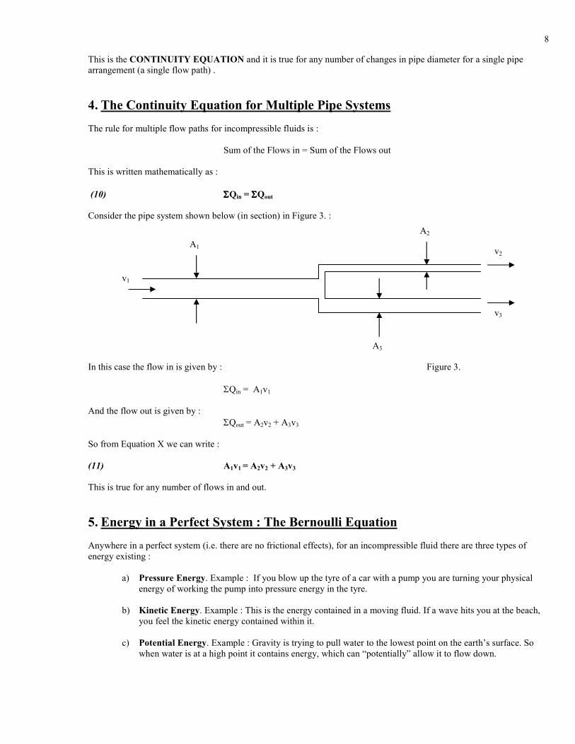
4. The Continuity Equation for Multiple Pipe Systems
The rule for multiple flow paths for incompressible fluids is :
Sum of the Flows in = Sum of the Flows out
This is written mathematically as :
(10) ΣΣΣΣQin = ΣΣΣΣQout
Consider the pipe system shown below (in section) in Figure 3. :
In this case the flow in is given by : Figure 3.
ΣQin = A1v1
And the flow out is given by :
ΣQout = A2v2 + A3v3
So from Equation X we can write :
(11) A1v1 = A2v2 + A3v3
This is true for any number of flows in and out.
5. Energy in a Perfect System : The Bernoulli Equation
Anywhere in a perfect system (i.e. there are no frictional effects), for an incompressible fluid there are three types of
energy existing :
a) Pressure Energy. Example : If you blow up the tyre of a car with a pump you are turning your physical
energy of working the pump into pressure energy in the tyre.
b) Kinetic Energy. Example : This is the energy contained in a moving fluid. If a wave hits you at the beach,
you feel the kinetic energy contained within it.
c) Potential Energy. Example : Gravity is trying to pull water to the lowest point on the earth’s surface. So
when water is at a high point it contains energy, which can “potentially” allow it to flow down.
A2
A1
A3
v2
v3
v1
9
At any point in a perfect system the sum of these “bits” of energy in different forms (Pressure, Kinetic and
Potential) must equal the sum of these “bits” at any other point in the system.
This is because energy cannot be “created” or “destroyed”, it can only change its form. This is what the BERNOULLI
EQUATION expresses.
Appendix 1. gives the derivation of the Kinetic Energy in terms of a pressure and Appendix 2. gives the derivation of the
Potential Energy in terms of a pressure.
These different forms of energy are expressed mathematically (as pressures) in the Bernoulli Equation (for a perfect
system) shown below :
(12) P1 + ½.ρρρρ.v12 + ρρρρ.g.h1 = P2 + ½.ρρρρ.v2
2 + ρρρρ.g.h2
The terms on the left hand side of the Equation are as follows :
P1 is the pressure energy at point 1 (expressed as a pressure). [Units are N/m2 or Pa]
ρ is the density of the fluid. [Units are Kg/m3]
v1 is the velocity of the fluid at point 1. [Units are m/s]
g is the acceleration due to earth’s gravity (9.81 m/s/s). [Units are m/s/s]
h1 is the height (from a given datum) of the fluid at point 1. [Units are m]
The terms are similar on the right hand side of the Equation, but for point 2.
The left hand side of the equation represents all the “bits” of energy (expressed as pressures) at a point 1 in a perfect
system and the right hand side all the “bits” of energy (expressed as pressures) at another point 2.
6. Imperfect Systems : Friction and the Bernoulli Equation
Of course in the real world, systems are not perfect. Energy is lost from a real system as friction. This is the sound and
heat generated by the fluid as it flows through the pipes. These forms of energy are lost by the fluid rubbing against the
walls of the pipe, rubbing against itself and by turbulence in the flow. The amount of frictional loss is affected by the
following parameters :
a) The length of the pipe. The longer the pipes the greater the frictional losses.
b) The roughness of the pipe walls. The smoother the surface of the pipe the smaller the frictional losses.
c) The diameter of the pipe. The smaller the diameter of the pipe the greater the frictional losses.
d) The velocity of the fluid. The greater the velocity of the fluid the greater the frictional losses.
e) The type of flow of the fluid. Turbulent flow creates greater friction losses than laminar flow.
f) Changes in the shape or section of the pipe. Fittings, valves, bends etc. all increase frictional losses.
Frictional losses are non-linear. This means that if you double one of the above parameters then the frictional losses can
triple or quadruple in size. Also if there is no flow there are no frictional losses. Appendix 3 gives a fuller explanation of
the relationship between the above variables.
Pressure
Energy as
a pressure
at point 1
Kinetic
Energy as
a pressure
at point 1
Potential
Energy as
a pressure
at point 1
10
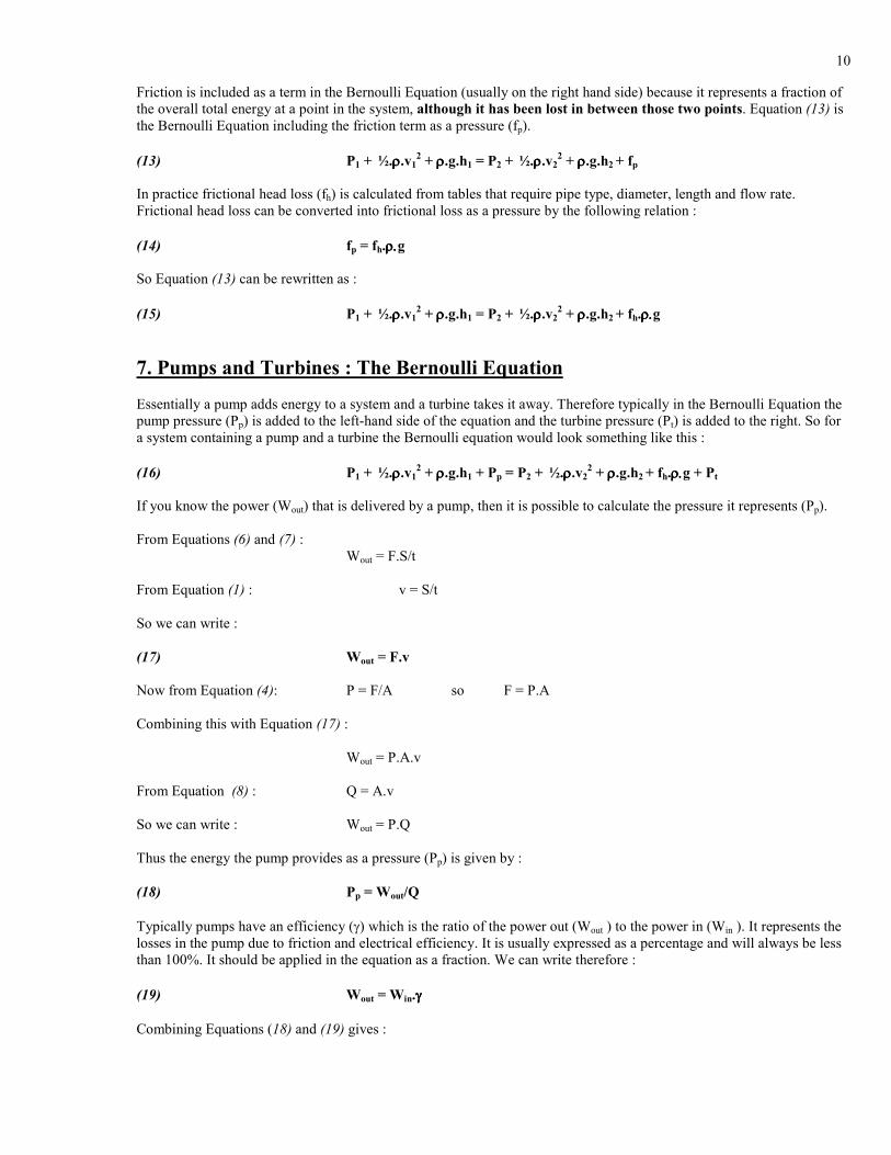
Friction is included as a term in the Bernoulli Equation (usually on the right hand side) because it represents a fraction of
the overall total energy at a point in the system, although it has been lost in between those two points. Equation (13) is
the Bernoulli Equation including the friction term as a pressure (fp).
(13) P1 + ½.ρρρρ.v12 + ρρρρ.g.h1 = P2 + ½.ρρρρ.v2
2 + ρρρρ.g.h2 + fp
In practice frictional head loss (fh) is calculated from tables that require pipe type, diameter, length and flow rate.
Frictional head loss can be converted into frictional loss as a pressure by the following relation :
(14) fp = fh.ρ.ρ.ρ.ρ.g
So Equation (13) can be rewritten as :
(15) P1 + ½.ρρρρ.v12 + ρρρρ.g.h1 = P2 + ½.ρρρρ.v2
2 + ρρρρ.g.h2 + fh.ρ.ρ.ρ.ρ.g
7. Pumps and Turbines : The Bernoulli Equation
Essentially a pump adds energy to a system and a turbine takes it away. Therefore typically in the Bernoulli Equation the
pump pressure (Pp) is added to the left-hand side of the equation and the turbine pressure (Pt) is added to the right. So for
a system containing a pump and a turbine the Bernoulli equation would look something like this :
(16) P1 + ½.ρρρρ.v12 + ρρρρ.g.h1 + Pp = P2 + ½.ρρρρ.v2
2 + ρρρρ.g.h2 + fh.ρ.ρ.ρ.ρ.g + Pt
If you know the power (Wout) that is delivered by a pump, then it is possible to calculate the pressure it represents (Pp).
From Equations (6) and (7) :
Wout = F.S/t
From Equation (1) : v = S/t
So we can write :
(17) Wout = F.v
Now from Equation (4): P = F/A so F = P.A
Combining this with Equation (17) :
Wout = P.A.v
From Equation (8) : Q = A.v
So we can write : Wout = P.Q
Thus the energy the pump provides as a pressure (Pp) is given by :
(18) Pp = Wout/Q
Typically pumps have an efficiency (γ) which is the ratio of the power out (Wout ) to the power in (Win ). It represents the
losses in the pump due to friction and electrical efficiency. It is usually expressed as a percentage and will always be less
than 100%. It should be applied in the equation as a fraction. We can write therefore :
(19) Wout = Win.γγγγ
Combining Equations (18) and (19) gives :
11
(20) Pp = Win.γγγγ/Q
This can be substituted into the Bernoulli Equation (16) and allows the determination of the pump power requirement or
alternatively the flow rate in a system for a given pump power.
Analysis of turbines will not be dealt with in detail here but is very similar to that of pumps (but in reverse).
8. Typical Scenarios
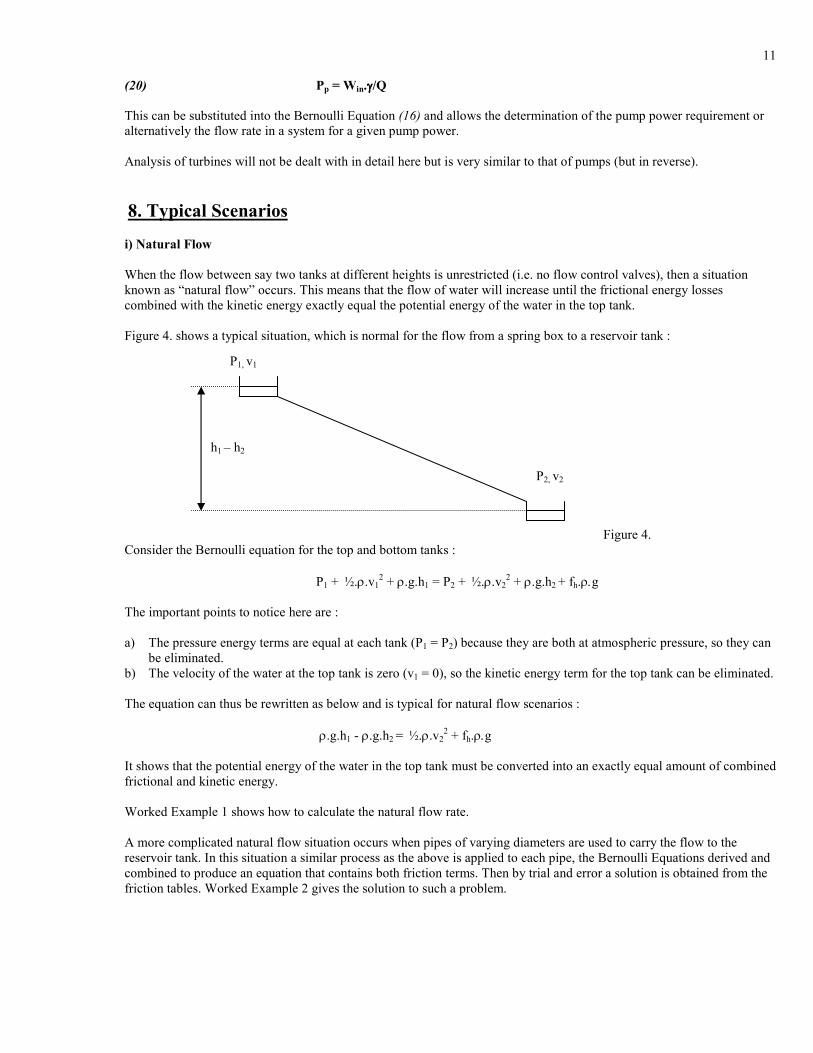
i) Natural Flow
When the flow between say two tanks at different heights is unrestricted (i.e. no flow control valves), then a situation
known as “natural flow” occurs. This means that the flow of water will increase until the frictional energy losses
combined with the kinetic energy exactly equal the potential energy of the water in the top tank.
Figure 4. shows a typical situation, which is normal for the flow from a spring box to a reservoir tank :
Figure 4.
Consider the Bernoulli equation for the top and bottom tanks :
P1 + ½.ρ.v12 + ρ.g.h1 = P2 + ½.ρ.v2
2 + ρ.g.h2 + fh.ρ.g
The important points to notice here are :
a) The pressure energy terms are equal at each tank (P1 = P2) because they are both at atmospheric pressure, so they can
be eliminated.
b) The velocity of the water at the top tank is zero (v1 = 0), so the kinetic energy term for the top tank can be eliminated.
The equation can thus be rewritten as below and is typical for natural flow scenarios :
ρ.g.h1 - ρ.g.h2 = ½.ρ.v22 + fh.ρ.g
It shows that the potential energy of the water in the top tank must be converted into an exactly equal amount of combined
frictional and kinetic energy.
Worked Example 1 shows how to calculate the natural flow rate.
A more complicated natural flow situation occurs when pipes of varying diameters are used to carry the flow to the
reservoir tank. In this situation a similar process as the above is applied to each pipe, the Bernoulli Equations derived and
combined to produce an equation that contains both friction terms. Then by trial and error a solution is obtained from the
friction tables. Worked Example 2 gives the solution to such a problem.
P2, v2
h1 – h2
P1, v1
12
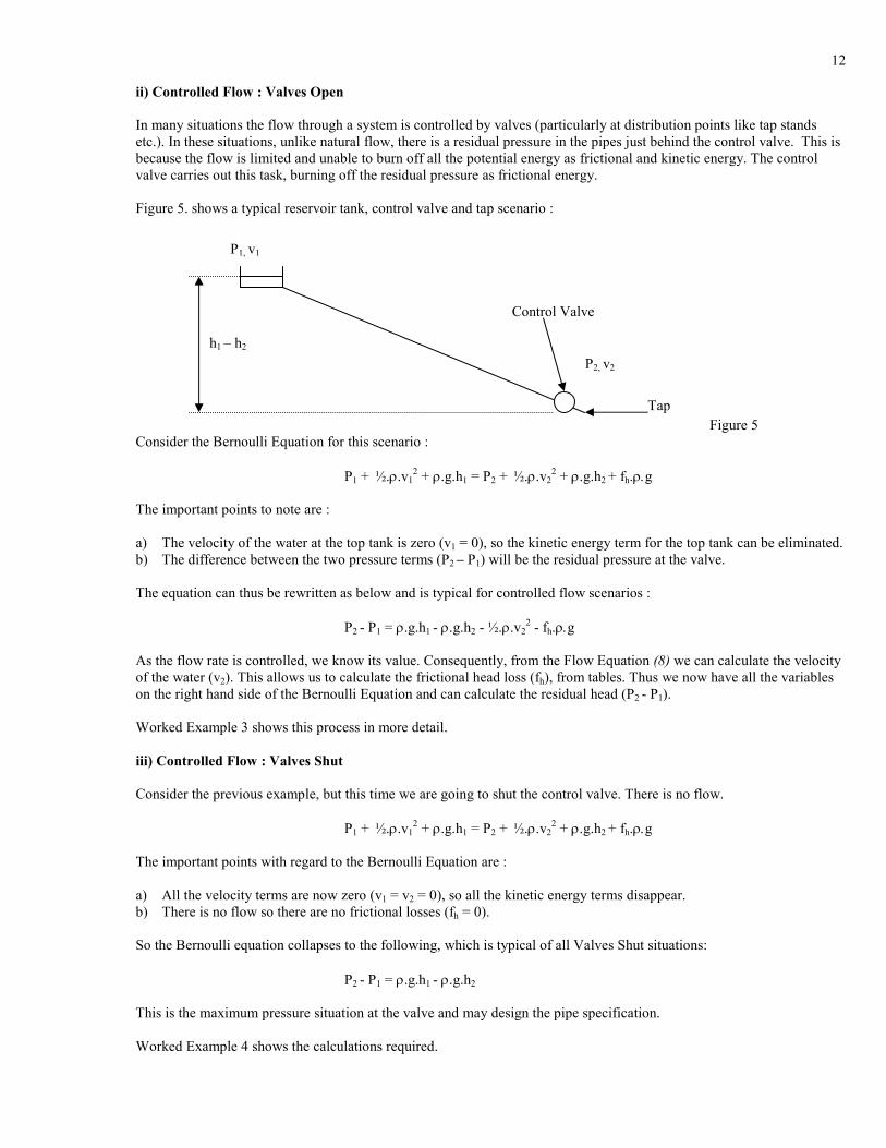
ii) Controlled Flow : Valves Open
In many situations the flow through a system is controlled by valves (particularly at distribution points like tap stands
etc.). In these situations, unlike natural flow, there is a residual pressure in the pipes just behind the control valve. This is
because the flow is limited and unable to burn off all the potential energy as frictional and kinetic energy. The control
valve carries out this task, burning off the residual pressure as frictional energy.
Figure 5. shows a typical reservoir tank, control valve and tap scenario :
Figure 5
Consider the Bernoulli Equation for this scenario :
P1 + ½.ρ.v12 + ρ.g.h1 = P2 + ½.ρ.v2
2 + ρ.g.h2 + fh.ρ.g
The important points to note are :
a) The velocity of the water at the top tank is zero (v1 = 0), so the kinetic energy term for the top tank can be eliminated.
b) The difference between the two pressure terms (P2 – P1) will be the residual pressure at the valve.
The equation can thus be rewritten as below and is typical for controlled flow scenarios :
P2 - P1 = ρ.g.h1 - ρ.g.h2 - ½.ρ.v22 - fh.ρ.g
As the flow rate is controlled, we know its value. Consequently, from the Flow Equation (8) we can calculate the velocity
of the water (v2). This allows us to calculate the frictional head loss (fh), from tables. Thus we now have all the variables
on the right hand side of the Bernoulli Equation and can calculate the residual head (P2 - P1).
Worked Example 3 shows this process in more detail.
iii) Controlled Flow : Valves Shut
Consider the previous example, but this time we are going to shut the control valve. There is no flow.
P1 + ½.ρ.v12 + ρ.g.h1 = P2 + ½.ρ.v2
2 + ρ.g.h2 + fh.ρ.g
The important points with regard to the Bernoulli Equation are :
a) All the velocity terms are now zero (v1 = v2 = 0), so all the kinetic energy terms disappear.
b) There is no flow so there are no frictional losses (fh = 0).
So the Bernoulli equation collapses to the following, which is typical of all Valves Shut situations:
P2 - P1 = ρ.g.h1 - ρ.g.h2
This is the maximum pressure situation at the valve and may design the pipe specification.
Worked Example 4 shows the calculations required.
P2, v2
h1 – h2
P1, v1
Control Valve
Tap
13
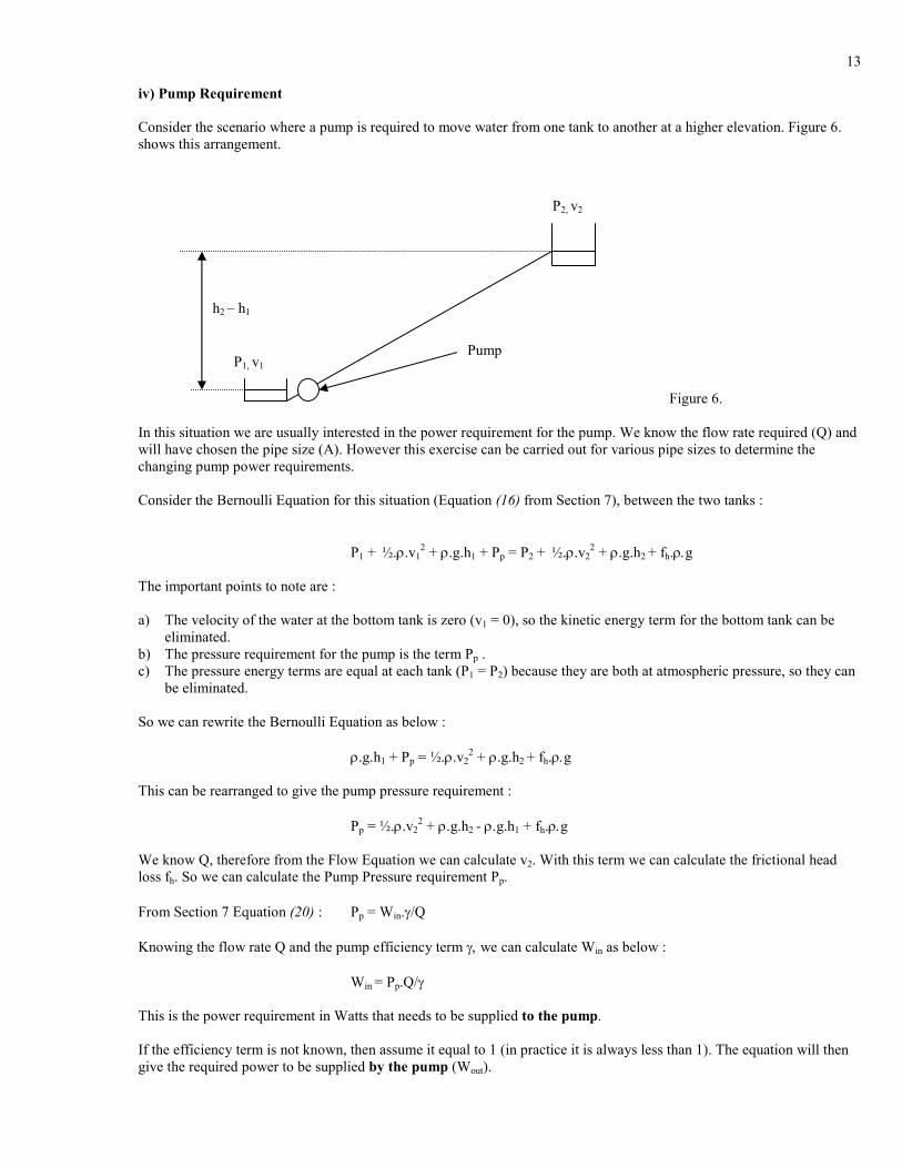
iv) Pump Requirement
Consider the scenario where a pump is required to move water from one tank to another at a higher elevation. Figure 6.
shows this arrangement.
Figure 6.
In this situation we are usually interested in the power requirement for the pump. We know the flow rate required (Q) and
will have chosen the pipe size (A). However this exercise can be carried out for various pipe sizes to determine the
changing pump power requirements.
Consider the Bernoulli Equation for this situation (Equation (16) from Section 7), between the two tanks :
P1 + ½.ρ.v12 + ρ.g.h1 + Pp = P2 + ½.ρ.v2
2 + ρ.g.h2 + fh.ρ.g
The important points to note are :
a) The velocity of the water at the bottom tank is zero (v1 = 0), so the kinetic energy term for the bottom tank can be
eliminated.
b) The pressure requirement for the pump is the term Pp .
c) The pressure energy terms are equal at each tank (P1 = P2) because they are both at atmospheric pressure, so they can
be eliminated.
So we can rewrite the Bernoulli Equation as below :
ρ.g.h1 + Pp = ½.ρ.v22 + ρ.g.h2 + fh.ρ.g
This can be rearranged to give the pump pressure requirement :
Pp = ½.ρ.v22 + ρ.g.h2 - ρ.g.h1 + fh.ρ.g
We know Q, therefore from the Flow Equation we can calculate v2. With this term we can calculate the frictional head
loss fh. So we can calculate the Pump Pressure requirement Pp.
From Section 7 Equation (20) : Pp = Win.γ/Q
Knowing the flow rate Q and the pump efficiency term γ, we can calculate Win as below :
Win = Pp.Q/γ
This is the power requirement in Watts that needs to be supplied to the pump.
If the efficiency term is not known, then assume it equal to 1 (in practice it is always less than 1). The equation will then
give the required power to be supplied by the pump (Wout).
h2 – h1
P1, v1
Pump
P2, v2
14
As an aside, the power supplied to the pump (Win ) will be equal to the electrical power supplied. Electrical power (We) is
given by the following Equation :
(21) We = I.V
Where I is the current (in Amps) and V is the voltage (in Volts). Typically the voltage is known (power cables in Mexico
are approximately 110V, car batteries supply 12V) so it is possible to calculate the current requirement. This is useful for
specification of controllers, cables and fuses.
Worked Example 5 gives a typical calculation of pump requirements.
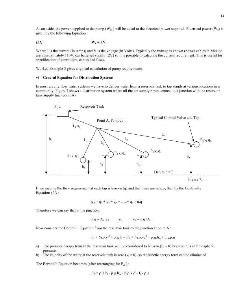
v) General Equation for Distribution Systems
In most gravity flow water systems we have to deliver water from a reservoir tank to tap stands at various locations in a
community. Figure 7 shows a distribution system where all the tap supply pipes connect to a junction with the reservoir
tank supply line (point A).
Figure 7.
If we assume the flow requirement at each tap is known (q) and that there are n taps, then by the Continuity
Equation (11) :
qA = q1 + q2 + q3 + …..+ qn = n.q
Therefore we can say that at the junction :
n.q = At .vA so vA = n.q /At
Now consider the Bernoulli Equation from the reservoir tank to the junction at point A :
Pt + ½.ρ.vt2 + ρ.g.ht = PA + ½.ρ.vA
2 + ρ.g.hA + ft-A.ρ.g
a) The pressure energy term at the reservoir tank will be considered to be zero (Pt = 0) because it is at atmospheric
pressure.
b) The velocity of the water at the reservoir tank is zero (vt = 0), so the kinetic energy term can be eliminated.
The Bernoulli Equation becomes (after rearranging for PA ) :
PA = ρ.g.ht - ρ.g.hA - ½.ρ.vA2 - ft-A.ρ.g
Pt, vt Reservoir Tank
Point A, PA vA qA
ht
Typical Control Valve and Tap
P3 v3 q3 P2 v2 q2 P1 v1 q1
Pn vn qn
Lt At
L1 L2
L3
Ln
h1
h2 h3
hn
Datum h = 0

15
The Bernoulli Equation from the junction A to any typical tap is :
PA + ½.ρ.vn2 + ρ.g.hA = Pn + ½.ρ.vn
2 + ρ.g.hn + fA-n.ρ.g
Simplifying this we get : Pn = PA + ρ.g.hA - ρ.g.hn - fA-n.ρ.g
Substitute the equation for PA into this equation and simplify:
Pn = ρ.g.ht - ρ.g.hn - ft-A.ρ.g - fA-n.ρ.g - ½.ρ.vA2
Dividing by ρ.g to convert into head :
(22) Pn/ρρρρ.g = ht - hn - ft-A - fA-n - ½.vA2/g
This is the General Equation for any tap in the distribution system. It allows us to calculate two things :
a) If we know the tap and the reservoir tank supply pipe sizes we can calculate the residual head at the tap (Pn/ρ.g).
b) Alternatively if we know the desirable residual head at the taps we can design the tap supply pipe size.
Worked Example 6 shows this process in more detail.
9. Special Scenarios
i) Parallel Pipes
Figure 8 shows a pipe network where the feeder pipe (1) divides into two pipes (2,3) of different diameters at point A and
rejoins at point B to become another pipe section (4).
Figure 8.
There are two important points here :
a) The flow into the junctions, must equal the flow out (see section 4. Equation (11)), so we can write :
A1v1 = A2v2 + A3v3 = A4v4
b) The pressure drop between points A and B in pipe 2 must equal the pressure drop between points A and B in
pipe 3. This because there must be continuity of pressure at point B. So if we wrote out the Bernoulli equations
between points A and B for each pipe (2,3)we would get :
For pipe 2 : PA + ½.ρ.v22 + ρ.g.hA = PB + ½.ρ.v2
2 + ρ.g.hB + fh2.ρ.g
For pipe 3 : PA + ½.ρ.v32 + ρ.g.hA = PB + ½.ρ.v3
2 + ρ.g.hB + fh3.ρ.g
Examination of these two equations and simplification shows that the frictional head losses must be equal :
A B A2,v2
A1, v1 A4,v4
A3, v3
16
fh2 = fh3
Knowing the two relations in a) and b) it is possible to calculate the velocities in pipes 2 and 3 by trial and error (using the
friction charts) and thus the pressure drop between A and B.
Worked Example 7 gives a typical calculation for parallel pipes.
ii) Water Sources At Different Elevations
Consider the scenario shown in Figure 9, where there are two water sources at different elevations joined together at point
A, which then supplies a reservoir tank at B.
Figure 9.
The important points to note are the following :
a) The pressures (P1, P2, P3) at all three tanks are equal (atmospheric).
b) The pressure at point A (PA) will be the same for all three pipes.
c) The velocities at the two top tanks will be zero (v1 = v2 = 0), so both of these kinetic energy terms disappear.
Typically the problem here is to design one of the source lines such that the pressure at the junction A is equalised. If the
pressure is not equalised in the design then the flows will interfere with each other.
Assume, therefore, that the required flows out of each source are known, which means v1A and v2A are fixed.
The Bernoulli Equations for the two sources to point A, are given below :
For source 1 : ρ.g.h1 = PA + ½.ρ.v1A2 + ρ.g.h3 + fh1-A.ρ.g
For source 2 : ρ.g.h2 = PA + ½.ρ.v2A2 + ρ.g.h3 + fh2-A.ρ.g
For source 1 the pressure at the junction can be calculated by rearranging the equation as below :
For source 1 : PA = ρ.g.h1 + ½.ρ.v1A2 + ρ.g.h3 + fh1-A.ρ.g
Knowing PA means we can work out the pipe size required to burn off the required amount of frictional head to equalise
the pressures at the junction.
From the Continuity Equation (11) we can calculate the combined flow of the two source pipes.
A3v3A = A1v1A + A2v2A
Now we can write the Bernoulli Equation from the junction to the reservoir tank :
PA + ½.ρ.v3A2 + ρ.g.h3 = P3 + ½.ρ.v3
2 + fhA-3.ρ.g
P3, v3
P1, v1
h1
h3
P2, v2
A
h2
B
v1A,v2A

17
Assuming that v3A = v3 (this means there is a control valve at the reservoir tank), then we can either calculate the residual
pressure at the control valve or calculate the pipe size required to reduce this residual pressure to close to zero (the
minimum possible pipe size).
For natural flow conditions the calculation becomes too complicated for a treatment in this document.
Worked Example 8 gives a typical calculation for sources at different elevations.
18
APPENDICES
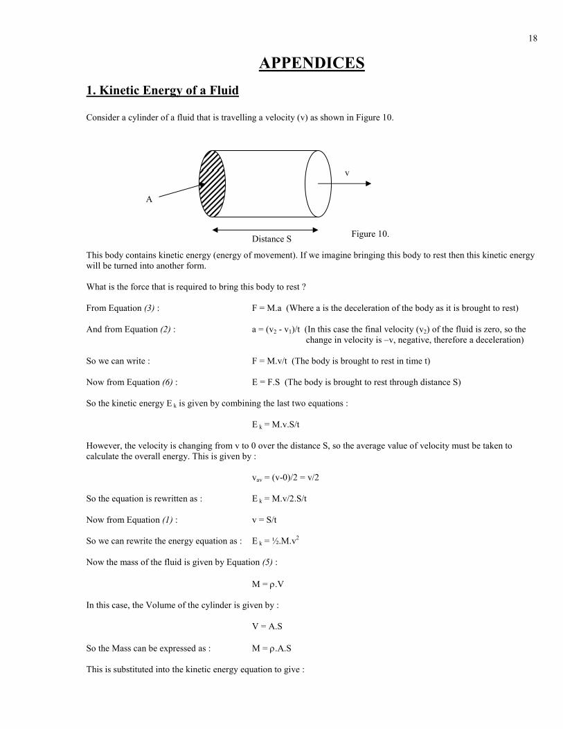
1. Kinetic Energy of a Fluid
Consider a cylinder of a fluid that is travelling a velocity (v) as shown in Figure 10.
Figure 10.
This body contains kinetic energy (energy of movement). If we imagine bringing this body to rest then this kinetic energy
will be turned into another form.
What is the force that is required to bring this body to rest ?
From Equation (3) : F = M.a (Where a is the deceleration of the body as it is brought to rest)
And from Equation (2) : a = (v2 - v1)/t (In this case the final velocity (v2) of the fluid is zero, so the
change in velocity is –v, negative, therefore a deceleration)
So we can write : F = M.v/t (The body is brought to rest in time t)
Now from Equation (6) : E = F.S (The body is brought to rest through distance S)
So the kinetic energy E k is given by combining the last two equations :
E k = M.v.S/t
However, the velocity is changing from v to 0 over the distance S, so the average value of velocity must be taken to
calculate the overall energy. This is given by :
vav = (v-0)/2 = v/2
So the equation is rewritten as : E k = M.v/2.S/t
Now from Equation (1) : v = S/t
So we can rewrite the energy equation as : E k = ½.M.v2
Now the mass of the fluid is given by Equation (5) :
M = ρ.V
In this case, the Volume of the cylinder is given by :
V = A.S
So the Mass can be expressed as : M = ρ.A.S
This is substituted into the kinetic energy equation to give :
A
v
Distance S

19
(23) E k = ½.ρρρρ.A.S.v2
In the Bernoulli equation, the energies are represented as pressures. From Equation (4) we get :
P = F/A
And from Equation (6) : E = F.S
Combining these two equations we get : P = E/(A.S)
So if we divide the kinetic energy Equation (23) by (A.S) we get it in terms of pressure :
P = ½.ρ.A.S.v2/(A.S)
The A.S terms cancel out to give the kinetic energy in terms of a pressure (Pk) :
(24) Pk = ½.ρρρρ.v2
This equation represents the kinetic energy of a fluid in terms of a pressure.
2. Potential Energy of a Fluid
Consider a column of a fluid of height h and area A, as shown in Figure 11.
To raise this column of water to a total height of h, means doing work against gravity. The force required to do this is
given by Equation III, except we replace the “a” term with the acceleration due to gravity “g” :
F = M.g
The mass of the column is given by Equation (5) :
M = ρ.A.h
Figure 11.
So we can rewrite the equation for the force required to raise this column of a fluid against gravity as :
A
h

20
F = ρ.A.h.g
Now from Equation (6), the amount of energy required to carry out this action is :
E = F.S
In this case not all the fluid is being raised to a height h, instead the average distance moved by the fluid is h/2 :
So we can write :
(25) Ep = ρρρρ.A.h.g.S where S = h/2
This is the potential energy (Ep )of the column.
In the Bernoulli equation, the energies are represented as pressures. From Equation (4) we get :
P = F/A
And from Equation (6) : E = F.S
Combining these two equations we get : P = E/(A.S)
So if we divide the potential energy Equation (25) by (A.S) we get it in terms of pressure :
(26) Pp = ρρρρ.g.h
This equation represents the potential energy of a fluid in terms of a pressure.
3. Friction Losses and the Reynolds Number
The frictional head loss for fluids flowing in pipes is calculated by the following equation :
(27) fh = f.L.v2/2.D.g
Where f is the friction factor (see below for calculation)
L is the pipe length (m)
v is the average fluid velocity (m/s)
D is the pipe diameter (m)
g is the acceleration due to gravity (9.81 m/s/s)
The only variable not available to us immediately is the frictional factor (f). This is dependent on the type of flow
occurring in the pipe. There are basically two types of flow (although there is a transition state between them ), these
are :
a) Laminar flow. Example : This is similar to the stream of smoke from a cigarette in still air. Close to the cigarette the
stream of smoke is very uniform and flowing evenly. This is laminar flow.
b) Turbulent flow. Example : This is when the stream of smoke from the cigarette becomes unstable, with whorls and
eddies. This state occurs in the stream of smoke after the laminar flow.
These two states of flow can be described by a dimensionless quantity (just a number) known as the Reynolds Number
(NRE). This number is calculated by the following formula :
(28) NRE = v.D/µµµµk
Where v is the average fluid velocity (m/s)
D is the pipe diameter (m)
µk is the kinematic viscosity of the fluid (m2/s), which is a measure of how ‘thick’ the fluid is.
21
If the Reynolds Number is less than 2000 then the fluid flow is laminar. In this case the friction factor (f) can be
calculated by the following equation :
(29) f = 64/ NRE
If the Reynolds Number is greater than 2000 then the fluid flow is turbulent. In this case the friction factor (f) can be
calculated by use of a Moody Chart.
4. Water System Design Parameters
The following are a list of design parameters that are important in the design of gravity-flow water systems :
1. Maximum Pressure Limits : The taps and valves closed state, should be the maximum pressure condition for the
system. Maximum head limits for the pipe work will be used to carry out the calculations. This scenario is used at the
start of the design to be able to place any break-pressure tanks that may be required.
2. Safe Yield : The safe yield is the minimum flow from the water source. It is important to not draw more than this
supply from the system at any point. If this happens then spring boxes and/or break pressure tanks will run dry and
air will enter the system.
3. Negative or Low Pressure Head : If the pressure head (P in the Bernoulli Equation) becomes negative at any point
in the system then two things may happen. Firstly a siphon effect is occurring which is trying to suck water into the
system. This is undesirable as polluted groundwater may be introduced into the system. Secondly, large negative
pressures can cause air to come out of solution in the water and cause air-blocks. Jordan [P.52] suggests that the
pressure head should, if possible, not fall below 10m (98100 Pa pressure) anywhere in the system and never go
negative.
4. Velocity Limits : The flow velocity in the pipelines should not be to great as particles suspended in the water will
cause excessive erosion. Also if the velocity is too low then these particles will settle out of the flow and may clog
the pipes at low points. This then requires washouts at low points in the system. Jordan [P.53] suggests that the
minimum velocity should be 0.7m/s and the maximum 3.0m/s.
5. Natural Flow : Natural Flow (see Section 8 i)) may be allowed to occur in the system at some sections of pipe.
Natural flow can be problematic in that the water velocity may exceed the limits set in parameter 4 above and/or
increase the flow rate above the safe yield parameter 2. Close attention should be made to these situations.
6. Residual Head : The residual head at a tap stand or valve is important. If it’s too high it will cause erosion of the
valve and if it is too low then the flow will be minimal. Jordan [P.141] suggests the following limits :
Absolute minimum : 7m
Low end of desired range : 10m
Most desirable : 15m
High end of desired range : 30m
Absolute maximum : 56m
7. Air-blocks : These occur when there are topographic features between the source and the collecting tank that are
lower than the collecting tank. Energy is lost from the system as these air-blocks are compressed and can result in no
flow. Jordan [P.55] gives the following design practices to avoid air-blocks :
♦ Arrange pipe sizes to minimise the frictional head loss between the source and the first air-block.
♦ Use larger-sized pipe at the top and smaller sized pipe at the bottom of the critical sections where air is going to
be trapped.
♦ The higher air blocks are the more critical ones and should be eliminated or minimised first.
♦ Air valves can be designed into the system to allow trapped air to escape.
22
8. Cost : Wherever possible smaller pipe diameters should be used, as they are cheaper. Combinations of pipes can
often produce cheaper solutions than using just one pipe size. However pipe lengths should be rounded to the nearest
100m length. Also the number of concrete structures such as break-pressure tanks should be minimised.
5. Interpolation
Introduction
Interpolation is a method for finding the value of a variable when non-linear data is provided at discrete points (i.e. we do
not know the mathematical function of the variable). It involves drawing straight lines between these discrete points and
then using the geometric rule for similar triangles to derive the value of a variable at a location between the discrete
points.
Theory
Consider the set of data below :
X Y
0 0
1 1
2 4
3 9
4 16
5 25
This data can be represented graphically as below :
0
5
10
15
20
25
30
0 1 2 3 4 5
Figure 12.
Imagine we want to find out what the value of Y is for a value of X = 2.4. If we know the function of X (in this case it is
X2) then it is easy Y = 2.4
2 = 5.76. But if we don’t know the function of X (which is more generally the case especially
with non-linear data) then how do we find the value for Y ? This is where we can use the approximate method known as
interpolation.
Interpolation assumes that we have drawn a straight line between points A and B above, this will give us the following
general situation (Figure 13.) :
A
B
23
Figure 13.
So how do we find Y3 knowing, X1, X2, X3, Y1 and Y2 ?
Well, we note that the triangles ABE and ACD are similar, that is they share the same angles. This means that the ratio of
their sides will be similar. So we can say :
Lengths CD/AD = BE/AE, this can be rewritten as :
(Y3 – Y1)/(X3 – X1) = (Y2 – Y1)/(X2 – X1)
We are trying to find Y3, so we can rearrange the above equation to isolate Y3.
(Y3 – Y1) = (Y2 – Y1)*(X3 – X1) /(X2 – X1)
and so :
Y3 = Y1 + (Y2 – Y1)*(X3 – X1) /(X2 – X1) (30)
This is the general interpolation equation.
We can use this equation to approximate the value of any function if we know the coordinates of the points either side
(X1, X2) and (Y1, Y2) and the X or Y coordinate of the point we are trying to find.
Example
Take the example in the theory section above for Y=X2.
What is the value of Y when X=2.4 ?
Answer : We know the following values : X1 = 2, X2 = 3, Y1 = 4, Y2 = 9 and X3 = 2.4. Substitute these into the
general interpolation equation (30) given above to give :
Y3 = 4 + (9 – 4)*(2.4 – 2) /(3 – 2)
And so, the approximation is Y3 = 6. The actual answer is 5.76 (see above), but this is not a bad approximation if
we did not know the function.
Notes
1. The above method should be used in the water pipe friction tables to estimate head losses.
2. The more data points the more accurate this method becomes.
3. The coordinates X1 and Y1 are always associated together, likewise for coordinates X2 and Y2. They define the
two discrete points on the curve.
A
B
X1 X2
Y1
Y2
Y3
X3
Y
X
C
D
E
Interpolated line
Actual line
24
Worked Examples
1. Natural flow
Consider a collector or spring tank at an elevation h1, supplying a reservoir tank at an elevation h2.
Figure 14.
Taking the equation from Section 8 i) :
ρ.g.h1 - ρ.g.h2 = ½.ρ.v22 + fh.ρ.g
And assuming the kinetic energy term is negligible gives us :
ρ.g (h1 - h2) = fh.ρ.g
Simplifying gives us :
(31) h1 - h2 = fh
This means that for the natural flow condition the actual head (h1 - h2) must equal the frictional head (fh) “burned off” by the
pipe. This means scanning the frictional head loss chart (interpolating where necessary) to find the frictional head loss that
exactly equals the actual head for the given pipe diameter and length. The following numerical example will demonstrate this
process.
Numerical Example
A spring tank is 500m from a reservoir tank, the difference in height between the two is 5m. It is proposed to use 1” diameter
pipe to link the two, what will be the volumetric flow rate of the water assuming a natural flow situation ?
Answer
Knowing h1 - h2 = 5, we can write equation (31) as :
5 = fh
Now there are 500m of pipe and we are looking for a frictional head loss in the chart per 100m of pipe. So divide the actual
head loss by 5 (as we have 500m of pipe). So we are looking for the frictional head loss per 100m of 1m on the chart for 1” dia.
pipe.
Scanning the chart gives us the following values for 1” dia. pipe :
Flow Rate (LPS) Frictional Head Loss (m/100m)
P2
h1 – h2
P1
25
0.19 0.62
0.25 1.07
Using the interpolation method (see Appendix 5) we can find the flow rate to give us exactly 1m of frictional head loss per
100m of 1” dia. pipe.
The variables for the general interpolation equation (30) are given below :
X1 = 0.62, X2 = 1.07, Y1 = 0.19, Y2 = 0.25 and X3 = 1.
Substitute these into the general interpolation equation (30) to give :
Y3 = 0.19 + (0.25 – 0.19)*(1 – 0.62) /(1.07 – 0.62)
And so, the approximation is Y3 = 0.2406 which can be rounded up to 0.24 LPS.
This is the flow that will produce a frictional head loss of 5m over 500m of 1” dia. pipe and is therefore the natural flow rate of
the system.
2. Natural flow with pipes of different diameters and lengths
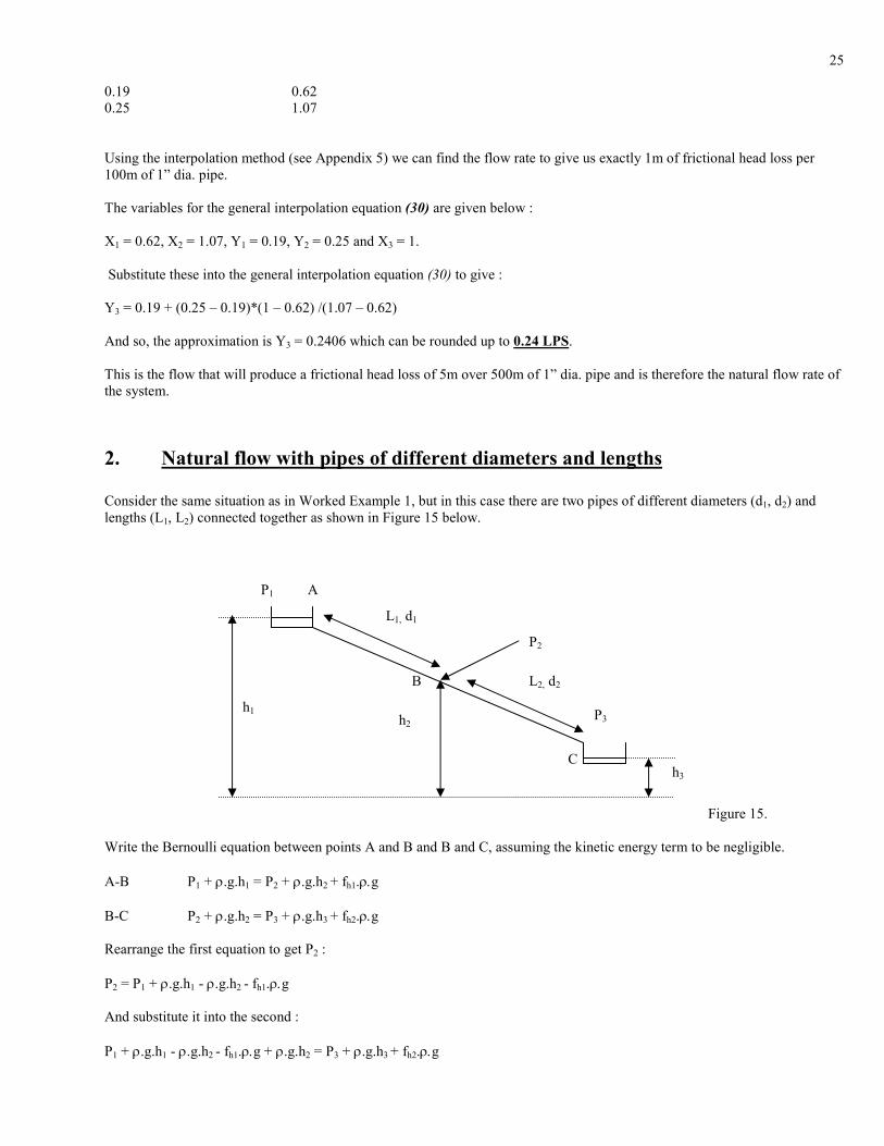
Consider the same situation as in Worked Example 1, but in this case there are two pipes of different diameters (d1, d2) and
lengths (L1, L2) connected together as shown in Figure 15 below.
Figure 15.
Write the Bernoulli equation between points A and B and B and C, assuming the kinetic energy term to be negligible.
A-B P1 + ρ.g.h1 = P2 + ρ.g.h2 + fh1.ρ.g
B-C P2 + ρ.g.h2 = P3 + ρ.g.h3 + fh2.ρ.g
Rearrange the first equation to get P2 :
P2 = P1 + ρ.g.h1 - ρ.g.h2 - fh1.ρ.g
And substitute it into the second :
P1 + ρ.g.h1 - ρ.g.h2 - fh1.ρ.g + ρ.g.h2 = P3 + ρ.g.h3 + fh2.ρ.g
P3 h1
P1
h2
h3
P2
L1, d1
L2, d2
A
B
C
26
Simplify, noting that P1= P3 (both are at atmospheric pressure), to give :
ρ.g.h1 - fh1.ρ.g = ρ.g.h3 + fh2.ρ.g
Rearrange to put actual head on one side and frictional head on the other :
ρ.g.h1 - ρ.g.h3 = fh1.ρ.g + fh2.ρ.g
Now divide by ρ.g to convert to heads :
(32) h1 - h3 = fh1 + fh2
This is the general equation for two pipes of different diameters and lengths joined together in a natural flow situation.
It should be noted that for any number of pipes n, with a total difference in head between the top and bottom tanks of ∆h, the
general equation can be written :
(33) ∆∆∆∆h = fh1 + fh2 + fh3 + ….. + fhn
So we can say that for any number of pipes n, the sum of the frictional head losses for each pipe, at some given flow rate Q will
be equal to the total difference in head between the top and bottom tanks.
Numerical Example
A spring tank is 200m from a reservoir tank, the difference in height between the two is 10m. It is proposed to use 100m of ½”
dia. pipe and 100m of 1” dia. pipe to link the two, what will be the volumetric flow rate of the water assuming a natural flow
situation ?
Answer
Knowing h1 - h3 is 10m we can substitute this into equation (32) to give us :
10 = fh1 + fh2
As both the ½” and 1” dia. pipes are 100m long we can compare the friction chart directly with the actual head of 10m.
The friction chart gives us the following range of data :
Flow Rate (LPS) Frictional Head Loss (m/100m) ½” dia. Frictional Head Loss (m/100m) 1” dia. Total (m)
0.06 1.05 0.09 1.14
0.13 3.77 0.30 4.07
0.19 7.99 0.62 8.61
0.25 13.61 1.07 14.68
Studying this data we can see that the natural flow rate lies somewhere between 0.19 and 0.25 as the total frictional head
“burned off” is 10 m and the limits either side of this are 8.61m and 14.68m. We need to interpolate to find the correct answer.
Using the interpolation method (see Appendix 5) we can find the flow rate to give us exactly 10m of frictional head loss for the
combination of pipes
The variables for the general interpolation equation (30) are given below :
X1 = 8.61, X2 = 14.68, Y1 = 0.19, Y2 = 0.25 and X3 = 10.00.
Substitute these into the general interpolation equation (30) to give :
Y3 = 0.19 + (0.25 – 0.19)*(10.00 – 8.61) /(14.68 – 8.61)

27
And so, the approximation is Y3 = 0.2037 which can be rounded down to 0.20 LPS.
This is the flow that will produce a frictional head loss of 10m over a combination of 100m of ½” dia. pipe and 100m of 1” dia.
pipe and is therefore the natural flow rate of the system.
3. Simple tap system (tap open)
Consider a similar situation to Worked Example 1, except that a control valve has been inserted into the line, immediately
before the discharge point (a tap).
Figure 16.
Taking the equation from Section 8 ii) :
P2 - P1 = ρ.g.h1 - ρ.g.h2 - ½.ρ.v22 - fh.ρ.g
Assuming the kinetic energy term to be negligible and rewriting P2 - P1 as the residual pressure at the valve or ∆P we get :
∆P = ρ.g.(h1 - h2) - fh.ρ.g
If we divide by ρ.g, then we can convert this equation from pressure (Pa) to head (m) :
(34) ∆∆∆∆H = (h1 - h2) - fh
Where ∆H is the residual head at the valve.
Numerical Example
A reservoir tank is 100m from a valve and tap arrangement, the difference in height between the two is 5m. It is proposed to
use 100m of 1” dia. pipe to link the two. Assuming the volumetric flow rate of the water is set by adjusting the valve to
0.25LPS, what is the residual head at the valve ?
Answer
Knowing h1 – h2 is 5m we can substitute this into equation (34) to give us :
∆H = 5 - fh
Now we know the volumetric flow rate is set at 0.25LPS, so consulting the friction chart for 1” diameter pipe we find that the
frictional head loss is 1.07m/100m for this flow rate. We have 100m of pipe, so therefore the head loss (fh) is 1.07m.
This means that the residual head at the valve is :
∆H = 5 – 1.07 = 3.93m
See Appendix 4 Part 6 for the acceptable residual heads at valves and taps.
P2
h1 – h2
P1
Control Valve
Tap

28
4. Simple tap system (tap closed)
Consider Worked Example 3 and Figure 16, except that in this case the control valve has been shut.
Taking the equation from Section 8 iii), we have :
P2 - P1 = ρ.g.h1 - ρ.g.h2
We can rewrite P2 - P1 as the maximum static pressure at the valve (Pmax) and divide by ρ.g to convert this equation from
pressure (Pa) to head (m) to give the maximum static head Hmax:
(35) Hmax = h1 - h2
In any system the maximum static head is generally given by the difference in height from the source to the lowest point of the
system.
Numerical Example
Taking the previous numerical example (3), what is the maximum static head if the tap is closed ?
Answer
Knowing h1 – h2 is 5m we can substitute this into equation (35) to give us :
Hmax = 5
The maximum static head in the system is at the point of greatest difference in height between the source and any other point.
In this case that other point is at the tap and is 5m.
5. Pump requirement
Consider the arrangement of a collector tank, pump and reservoir tank shown in Figure 17.
Figure 17.
Taking the pump pressure requirement equation from Section 8 iv) :
Pp = ½.ρ.v22 + ρ.g.h2 - ρ.g.h1 + fh.ρ.g
h2 – h1
P1
Pump
P2
29
And assuming the kinetic energy term is negligible gives us :
(36) Pp = ρρρρ.g.(h2 - h1+ fh)
This is the general equation for calculating the pressure requirement for a pump.
Combined with two other equations (20) which gives the power that needs to be supplied to the pump (Win)
Win = Pp .Q/γ
and (21) which gives the electrical power required (We)
We = I.V
it is possible to derive the pump specification for a series of different diameter delivery pipes, assuming a given volumetric
flow rate.
Numerical Example
A reservoir tank is 100m uphill from a water source, the difference in height between the two is 20m. It is proposed to use a
pump to push the water up to the reservoir tank at a flow rate of 0.5LPS. Two pipe diameters of ½” and 1” are available to link
the two. What size pumps are required (in Watts) for each pipe diameter, assuming a pump efficiency of 50% and what
electrical current is required assuming the smaller pump is chosen and we are stealing the electricity from a 110V pylon ?
Answer
We need to find the required pump pressure for each diameter of delivery pipe. We know the difference in height between the
source and the reservoir tank (h2 - h1) is 20m. For a flow rate of 0.5LPS the frictional head loss chart gives the following results
for ½” and 1” dia. pipes :
Flow Rate (LPS) Frictional Head Loss (m/100m) ½” dia. Frictional Head Loss (m/100m) 1” dia.
0.5 49.14 3.86
As we have 100m of pipe in each case these values can be inserted directly into equation (36) to give the pump pressure
requirement :
For ½” dia. pipe : For 1” dia. pipe :
Pp = 1000*9.81(20 + 49.14) = 678263.4 Pa Pp = 1000*9.81(20 + 3.86) = 234066.6 Pa
Taking the density of water as ρ = 1000 Kg/m3 and the acceleration due to gravity as g = 9.81m/s/s.
These two pump pressures can now be inserted into equation (20) to give the pump power requirement, taking the pump
efficiency (γ) as 0.5 and converting the volumetric flow rate (Q) from LPS to m3/s :
For ½” dia. pipe : For 1” dia. pipe :
Win = 678263.4*0.0005/0.5 = 678.3 Watts Win = 234066.6*0.0005/0.5 = 234.1 Watts
Note that the power requirement for the 1” dia. delivery pipe is less than half of that for the ½“ dia. pipe.
Taking the smaller pump (for the 1” dia. delivery pipe) and using equation (21) we get a electrical current requirement (I) of :
I = We/V
Assuming no electrical losses We = Win, so :
I = 234.1/110 = 2.13 Amps

30
6. Distribution systems : the general equation
Consider a reservoir tank distribution system of the form shown in Figure 18 below.
Figure 18.
The general equation (22) for the residual head for any tap in the distribution system is derived in Section 8 v) :
Pn/p.g = ht - hn - ft-A - fA-n - ½.vA2/g
If we assume the kinetic energy term is negligible and write the residual head at any tap as Hn, then we get :
(37) Hn = ht - hn - ft-A - fA-n
This is the simplified general equation for the residual head of any tap in a distribution system of the form shown in Figure 18.
Numerical Example
A reservoir tank is at an elevation of 40m above a community that requires 3 public tap stands, each giving a flow of 0.25LPS.
The tank supply line has been laid and is 100m of 1” dia. pipe. The preferred residual head at each tap is 10m, the minimum
residual head is 7m and the topographic survey results are as follows :
Tap site no. Height above datum (m) Distance from supply line junction (m)
1 2 50
2 20 100
3 7 100
What are the optimum diameter pipes that should be used for each tap and what are the residual heads at each tap ?
Answer
First of all we need to calculate the overall flow rate through the supply line, this is given by :
qA = q1 + q2 + q3 = n.q
Pt Reservoir Tank
Point A, PAqA
ht
Typical Control Valve and Tap
P3 q3 P2 q2 P1 q1
Pn qn
Lt At
L1 L2
L3
Ln
h1
h2 h3
hn
31
Where n is the number of taps and q is the maximum flow through each tap. So :
qA = 3*0.25 = 0.75LPS
Calculate the frictional head loss in the 100m of 1” dia. supply pipe due to a flow rate of 0.75LPS.
The friction tables give us the following data :
Flow Rate (LPS) Frictional Head Loss (m/100m)
0.69 6.96
0.76 8.19
Using the interpolation method (see Appendix 5) we can find frictional head loss for a flow rate of 0.75LPS.
The variables for the general interpolation equation (30) are given below :
X1 = 0.69, X2 = 0.76, Y1 = 6.96, Y2 = 8.19 and X3 = 0.75.
Substitute these into the general interpolation equation (30) to give :
Y3 = 6.96 + (8.19 – 6.96)*(0.75 – 0.69)/(0.76 – 0.69)
And so, the approximation is Y3 = 8.014m/100m which can be rounded up to 8.01 m/100m.
As we have 100m of pipe, we can say :
ft-A = 8.01m
We can now substitute this value and the height of the tank into the general equation (37) above to give :
Hn = 40 - hn – 8.01 - fA-n = 31.99 - hn - fA-n
If we assume we are trying to achieve an optimum residual head at each tap of 10m, then we can substitute this value as Hn in
the above equation and rearrange it to give the required frictional head loss fA-n in each distribution pipe.
fA-n = 31.99 - hn – 10 = 21.99 - hn
So for each pipe in tabular form :
Tap site no. Height above datum (m) Required frictional head loss (m) to give 10m of residual head
1 2 19.99
2 20 1.99
3 7 14.99
Consider tap 1.
Examination of the friction chart shows us that the highest frictional loss for a flow of 0.25LPS is for a ½” dia. pipe and is
13.61m/100m. In this case we have 50m of pipe, so the actual head loss is :
fA-1 = 13.61*50/100 = 6.81 m
This is the best we are going to do so we will select 50m of ½” dia. pipe giving us a residual head at tap 1 of :
Hn = 31.99 – 2.00 – 6.81 = 23.18 m
32
Consider tap 2.
Examination of the friction chart gives us the following frictional head losses for a flow rate of 0.25LPS :
Diameter Frictional head loss (m/100m)
½” 13.61
¾ ” 3.47
1” 1.07
1¼ “ 0.28
We require a head loss of 1.99m and we have 100m of pipe, so it is clear that the 1” dia. pipe is closest.
We will therefore select 100m of 1” dia. pipe giving us a residual head at tap 2 of :
Hn = 31.99 – 20.00 – 1.07 = 10.92 m
Consider tap 3.
Examination of the friction chart shows us that the highest frictional loss for a flow of 0.25LPS is for a ½” dia. pipe and is
13.61m/100m. In this case we have 100m of pipe, so the actual head loss is :
fA-3 = 13.61m
This is the best we are going to do so we will select 100m of ½” dia. pipe giving us a residual head at tap 1 of :
Hn = 31.99 – 7.00 – 13.61 = 11.38 m
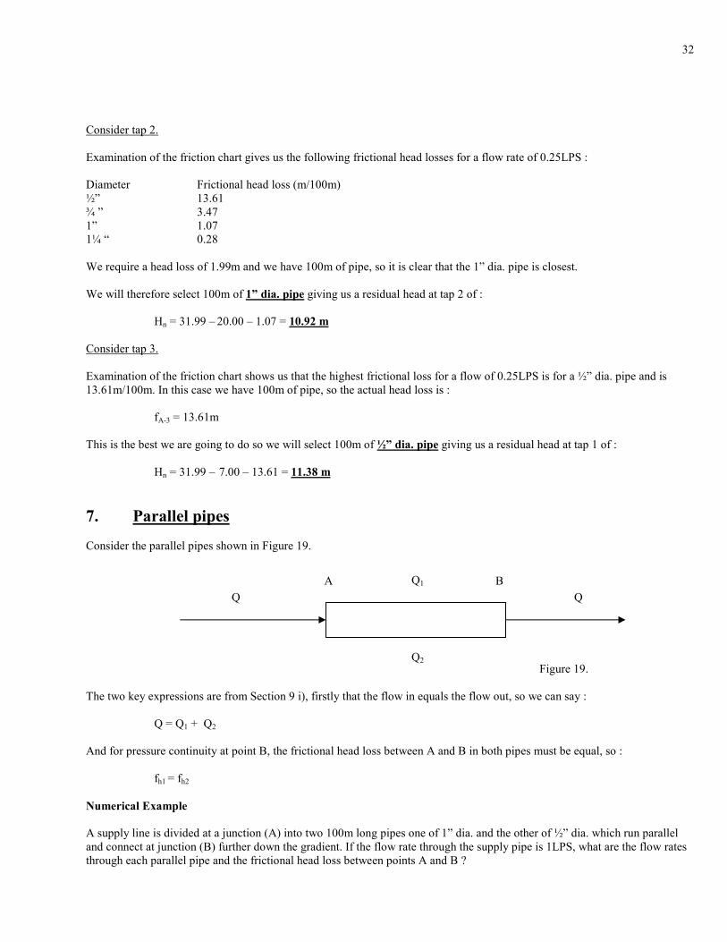
7. Parallel pipes
Consider the parallel pipes shown in Figure 19.
Figure 19.
The two key expressions are from Section 9 i), firstly that the flow in equals the flow out, so we can say :
Q = Q1 + Q2
And for pressure continuity at point B, the frictional head loss between A and B in both pipes must be equal, so :
fh1 = fh2
Numerical Example
A supply line is divided at a junction (A) into two 100m long pipes one of 1” dia. and the other of ½” dia. which run parallel
and connect at junction (B) further down the gradient. If the flow rate through the supply pipe is 1LPS, what are the flow rates
through each parallel pipe and the frictional head loss between points A and B ?
A B Q1
Q Q
Q2
33
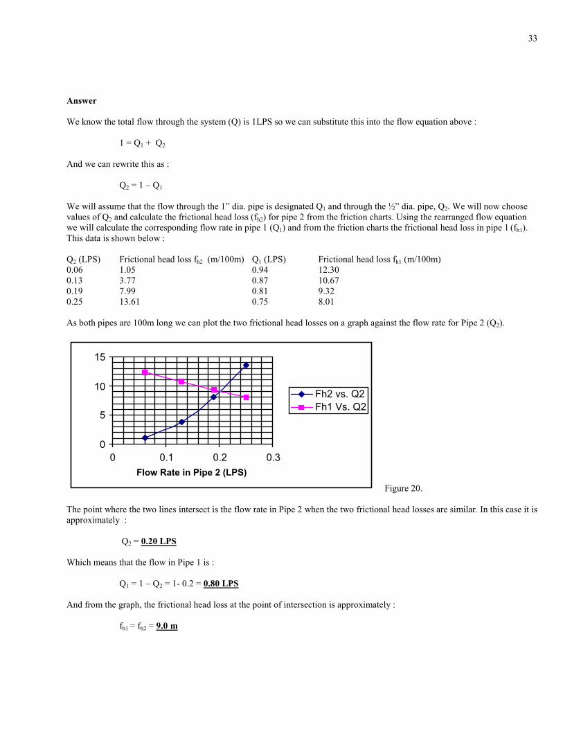
Answer
We know the total flow through the system (Q) is 1LPS so we can substitute this into the flow equation above :
1 = Q1 + Q2
And we can rewrite this as :
Q2 = 1 – Q1
We will assume that the flow through the 1” dia. pipe is designated Q1 and through the ½” dia. pipe, Q2. We will now choose
values of Q2 and calculate the frictional head loss (fh2) for pipe 2 from the friction charts. Using the rearranged flow equation
we will calculate the corresponding flow rate in pipe 1 (Q1) and from the friction charts the frictional head loss in pipe 1 (fh1).
This data is shown below :
Q2 (LPS) Frictional head loss fh2 (m/100m) Q1 (LPS) Frictional head loss fh1 (m/100m)
0.06 1.05 0.94 12.30
0.13 3.77 0.87 10.67
0.19 7.99 0.81 9.32
0.25 13.61 0.75 8.01
As both pipes are 100m long we can plot the two frictional head losses on a graph against the flow rate for Pipe 2 (Q2).
0
5
10
15
0 0.1 0.2 0.3
Flow Rate in Pipe 2 (LPS)
Fh2 vs. Q2
Fh1 Vs. Q2
Figure 20.
The point where the two lines intersect is the flow rate in Pipe 2 when the two frictional head losses are similar. In this case it is
approximately :
Q2 = 0.20 LPS
Which means that the flow in Pipe 1 is :
Q1 = 1 – Q2 = 1- 0.2 = 0.80 LPS
And from the graph, the frictional head loss at the point of intersection is approximately :
fh1 = fh2 = 9.0 m
34
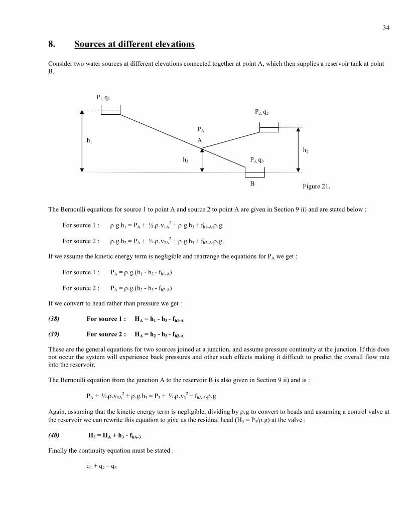
8. Sources at different elevations
Consider two water sources at different elevations connected together at point A, which then supplies a reservoir tank at point
B.
Figure 21.
The Bernoulli equations for source 1 to point A and source 2 to point A are given in Section 9 ii) and are stated below :
For source 1 : ρ.g.h1 = PA + ½.ρ.v1A2 + ρ.g.h3 + fh1-A.ρ.g
For source 2 : ρ.g.h2 = PA + ½.ρ.v2A2 + ρ.g.h3 + fh2-A.ρ.g
If we assume the kinetic energy term is negligible and rearrange the equations for PA we get :
For source 1 : PA = ρ.g.(h1 - h3 - fh1-A)
For source 2 : PA = ρ.g.(h2 - h3 - fh2-A)
If we convert to head rather than pressure we get :
(38) For source 1 : HA = h1 - h3 - fh1-A
(39) For source 2 : HA = h2 - h3 - fh2-A
These are the general equations for two sources joined at a junction, and assume pressure continuity at the junction. If this does
not occur the system will experience back pressures and other such effects making it difficult to predict the overall flow rate
into the reservoir.
The Bernoulli equation from the junction A to the reservoir B is also given in Section 9 ii) and is :
PA + ½.ρ.v3A2 + ρ.g.h3 = P3 + ½.ρ.v3
2 + fhA-3.ρ.g
Again, assuming that the kinetic energy term is negligible, dividing by ρ.g to convert to heads and assuming a control valve at
the reservoir we can rewrite this equation to give us the residual head (H3 = P3/ρ.g) at the valve :
(40) H3 = HA + h3 - fhA-3
Finally the continuity equation must be stated :
q1 + q2 = q3
P3, q3
P1, q1
h1
h3
P2, q2
A
h2
B
PA

35
Numerical Example
Consider a water system identical to that shown in Figure 21. The pipeline from spring tank 1 to the reservoir tank 3 has been
laid and consists of 1100m of 1” dia. pipe. It has been decided to “Tee” in a second water source, spring tank 2, at a point in the
mainline 100 m from spring tank 1, and at an altitude of 80m. This new pipeline is 100m long. Spring tank 1 at an altitude of
100m, has a safe yield of 0.2LPS and spring tank 2, at an altitude of 110m, a safe yield of 0.3LPS. The reservoir tank has a
control valve at the pipeline exit, an altitude of 0m and represents the altitude datum line. What diameter (or combination of
diameters) of pipe would be the optimum in order to supply the required flow rate to the reservoir tank and what is the residual
pressure at the control valve ?
Answer
First of all we must calculate the pressure head at point A (HA) by taking equation (38) for Source 1 :
HA = h1 - h3 - fh1-A
The required flow rate through this 100m section of 1” dia. pipe, is 0.2LPS, so from the friction charts we can find the
frictional head loss (fh1-A) by interpolation (see Appendix 5). This is approximately 0.7m. Substitute this into the above
equation along with the relevant altitudes to get the pressure head at point A :
HA = 100 - 80 – 0.7 = 19.3m
Now substituting this value into equation (39) for Source 2 we get :
For source 2 : 19.3 = 110 - 80 - fh2-A
Which means that the required frictional head loss in the 100m of pipe between point A and the spring tank 2 (fh2-A) is :
fh2-A = 110 - 80 – 19.3 = 10.7m
The required flow rate is 0.3LPS, so what will each diameter of pipe burn off, the data is shown below :
Pipe Dia. (in) Frictional head loss (m) for 100m of pipe at a flow rate of 0.3LPS
½ “ 18.58
¾” 4.73
1” 1.47
It is clear that we will have to use a combination of pipe diameters to achieve a frictional head loss close to 10.7m. In this case
the combination of ½” and ¾” diameters would be optimum.
The combination pipes equation is given in Jordan [P.203 Technical Appendix C] and is stated below :
(41) X = {100.H – (fhl .L)}/{fhs - fhl}
Where : X = Length of smaller diameter pipe, to give desired frictional head loss (m).
H = Desired frictional head loss (m).
fhl = Frictional head loss due to larger diameter pipe (m/100m).
fhs = Frictional head loss due to smaller diameter pipe (m/100m).
L = Total length of pipe (m).
In this case our desired head loss (H) is 10.7m, L = 100m, fhl = 4.73m/100m and fhs = 18.58m/100m (from above), so :
X = {100*10.7 – (4.73 *100)}/{18.58 – 4.73} = 43.10m
So we should employ 43.10m of ½” dia. pipe and 56.90m of 1” dia. pipe in order to get pressure continuity at point A.
Finally we need to find the residual head at the reservoir tank valve at point B.

36
By the continuity equation for flow rates :
q1 + q2 = q3
We can say that the flow rate along the pipe from A to B is :
q3 = 0.2 + 0.3 = 0.5LPS
The frictional head loss for this flow rate through 1” dia. pipe is from the charts, 3.86m/100m, so for 1000m of pipe the head
loss is :
fhA-3 = 3.86*1000/100 = 38.6m
Substitute this value, the pressure head at point A (HA above) and the height of point A (h3) into equation (40) to get the
residual head H3 at the reservoir valve :
H3 = 19.3 + 80 – 38.6 = 60.7m
9. Sample water system design
Numerical Example
Figure 22 below shows the topographic survey results for a proposed gravity flow water system.
Topographic Survey
0
50
100
150
200
0 500 1000 1500 2000 2500 3000
Distance from spring (m)
1. Spring
2.
3.
4. Reservoir Tank
Figure 22.
Assuming that the allowable pipe pressure head is 100m, the safe yield from the spring is 0.25LPS and that the design
parameters from Jordan are adhered to (see Appendix 4.), design a system that will supply water to the community for the
minimum cost.
Answer

37
The design of this water system will be approached in the following phases :
1. Requirement for and placement of break pressure tanks.
2. Design of pipe work.
3. Check chosen pipe work for low pressure head parameter.
1. Requirement for and placement of break pressure tanks
Consider the control valve at the reservoir tank being closed to begin with. This is the maximum static head condition
(Appendix 4 No. 1). All the static heads can be calculated from equation (35) below :
Hmax = h1 - h2
Consider the section of the system from the spring (point 1) to low point 2. The static head is :
Hmax 1-2 = 200 – 50 = 150m which exceeds the 100m allowable pipe pressure head given above.
Consider the section of the system from the spring (point 1) to high point 3. The static head is :
Hmax 1-3 = 200 – 125 = 75m which is within the above limit.
Consider the section of the system from the high point 3 to the reservoir tank (point 4). The static head is :
Hmax 3-4 = 125 - 0 = 125m which exceeds the 100m allowable pipe pressure head given above.
It is clear that the pipes at points 2 and 4 will blow unless we introduce break pressure tanks to relieve the pressure.
The first break pressure tank (hereafter BP1) must relieve the pressure at point 2 but still allow the water to flow over point 3.
The maximum height (hBP1) we can place BP1 at is given by :
hBP1 – h2 <= 100 so hBP1 – 50 <= 100 and therefore hBP1 <= 150
And hBP1 – h3 > 0 so hBP1 – 125 > 0 and therefore hBP1 > 125
So the height of BP1 must be less than or equal to 150 and greater than 125, to satisfy the conditions. As there will be frictional
losses in the pipes we should situate BP1 at its maximum allowable height, which is in this case 150m. This corresponds to a
location approximately 225m from the spring tank.
The second break pressure tank (hereafter BP2) must relieve the pressure at point 4 but not exceed the pressure head limits in
the pipe work between it and BP1.
The maximum height (hBP2) we can place BP2 at is given by :
hBP1 – hBP2 <= 100 so 150 - hBP2 <= 100 and therefore hBP2 >= 50
And hBP2 – h4 <= 100 so hBP2 – 0 <= 100 and therefore hBP2 <= 100
So the height of BP1 must be greater than or equal to 50 and less than or equal to 100, to satisfy the conditions. So it will be
placed at a height of 70m. This corresponds to a location approximately 2500m from the reservoir tank.
The two break pressure tank locations are added to the topographic survey, and shown below in Figure 23.

38
Topographic Survey
0
50
100
150
200
0 500 1000 1500 2000 2500 3000
Distance from spring (m)
Altitude (m)
1. Spring
2.
3.
4. Reservoir Tank
BP1BP2
Figure 23.
By inspection of Figure 23, the maximum static heads (after the introduction of the two break pressure tanks) are as follows :
At BP1 : Hmax BP1 = 200 - 150 = 50m
At Point 2 : Hmax 2 = 150 - 50 = 100m
At Point 3 : Hmax 3 = 150 - 125 = 25m
At BP2 : Hmax BP2 = 150 - 70 = 80m
At Point 4 : Hmax 4 = 70 - 0 = 70m
All of which are acceptable.
2. Design of pipe work
The safe yield of the water source is 0.25LPS. So in general we want to make sure that at no point in the system is more than
0.25LPS being drawn, as this will either empty a break pressure tank or the spring tank, allowing air into the system. We can
do this in two ways.
i) Design the natural flow situations such that just less than 0.25LPS is being drawn.
ii) Use control valves at the break pressure tanks and reservoir tank to limit the flow to just less than 0.25LPS.
We will consider the second option because the calculations are simpler and the control of the system easier.
Consider the section of pipe between the spring tank (point 1) and BP1 :
This section of pipe is 225m long and the maximum static head is 50m (see above). From the friction tables for a controlled
flow of 0.25LPS we get the following data.
Pipe Diameter Frictional head loss (m/100m) Frictional head loss for 225m of pipe (m) Velocity (m/s)
½” 13.61 30.62 1.28
¾ ” 3.47 7.81 0.73
1” 1.07 2.41 0.45
1¼ “ 0.28 0.63 0.26
It is clear that we can use ½” dia. pipe here, as it will not reduce the maximum static head below the 10m low pressure head
limit (see Appendix 4. No. 3) and the velocity of the water lies within acceptable parameters (see Appendix 4 No. 4).
The residual head at the BP1 valve (∆HBP1) is given by equation (34) :
39
∆HBP1 = (h1 – hBP1) - fh1-BP1
Substituting the numerical values into this equation for ½” dia. pipe we get :
∆HBP1 = (200 - 150) – 30.62 = 19.38m
This is an acceptable residual head based upon the limits set in Appendix 4 No. 6.
Consider the section of pipe between BP1 and BP2 :
This section of pipe is 2500 – 225 = 2375m long. The main feature we have to contend with is the topographical peak at point
3. This only lies 25m below BP1, so we can’t afford to “burn off” too much frictional head between BP1 and point 3 or else the
residual head will drop below the limit of 10m (see Appendix 4. No. 3). So we need to burn off no more than 25 - 10 = 15m of
head between BP1 and point 3.
The distance between BP1 and point 3 is from Figure 23, 1800 – 225 = 1575m. From the friction tables for a controlled flow of
0.25LPS we get the following data.
Pipe diameter Frictional head loss (m/100m) Frictional head loss for 1575m of pipe (m) Velocity (m/s)
½” 13.61 214.36 1.28
¾ ” 3.47 54.65 0.73
1” 1.07 16.85 0.45
1¼ “ 0.28 4.41 0.26
We clearly cannot use ½” and ¾” diameter pipes here as they “burn off” far more than 15m of head.
We could use 1¼ “ dia. pipe here, but there are two problems. Firstly the water velocity is very low at 0.26 m/s (see Appendix
4 No. 4) and secondly it is a little more costly than 1” dia. pipe (Appendix 4 No. 8).
So consider using 1” dia. pipe. The water velocity is still below the limit of 0.7 m/s (see Appendix 4 No. 4), but the head loss is
almost acceptable. There seems to be only one solution. Use 1” pipe between BP1 and point 3, and place a wash out at the
lowest point between BP1 and point 3, which happens to be point 2.
The pressure head at point 3 (H3) is given by equation (34) :
H3 = (hBP1 – h3) - fhBP1-3
Substituting the numerical values into this equation for 1” dia. pipe we get :
H3 = (150 - 125) – 16.85 = 8.15m
This is a little less than the minimum low pressure head limit of 10m (see Appendix 4 No. 3) but is acceptable in the
circumstances.
Now consider the second section of pipe between point 3 and BP2. The remaining pressure head is 8.15m (from above) and so
we can add this to the remaining head between point 3 and BP2 to get the overall head.
H3-BP2 = (125 – 70) + 8.15 = 63.15m
The most desirable residual head (Appendix 4 No.6) at a valve or tap is around 15m. So we are looking to “burn off”
something like :
fh3-BP2 = 63.15 – 15.00 = 48.15m
The distance between point 3 and BP2 is from Figure 23, 2500 – 1800 = 700m. From the friction tables for a controlled flow of
0.25LPS we get the following data.
40
Pipe diameter Frictional head loss (m/100m) Frictional head loss for 700m of pipe (m) Velocity (m/s)
½” 13.61 95.27 1.28
¾ ” 3.47 24.29 0.73
1” 1.07 7.49 0.45
1¼ “ 0.28 1.96 0.26
We clearly cannot use ½” diameter pipe here as it “burns off” far more than 48.15m of head.
¾ “ dia. pipe here looks good, as although it only burns off approximately half of the required head, it produces a water
velocity within the parameters required (Appendix 4 No. 4) and is cheaper than the 1” dia. pipe (Appendix 4 No. 8).
The residual head at the BP2 valve (∆HBP2) is given by :
∆HBP2 = H3 + (h3 – hBP2) - fh3-BP2
Substituting the numerical values into this equation for ¾ ” dia. pipe we get :
∆HBP2 = 8.15 + (125 - 70) – 24.29 = 38.86m
This is in the high end of the residual head range based upon the limits set in Appendix 4 No. 6.
We can improve on this and reduce costs by using a combination of ¾” dia. pipe and ½” dia. pipe. Consider the combination
pipes equation (41).
X = {100.H – (fhl .L)}/{fhs - fhl}
Where : X = Length of smaller diameter pipe, to give desired frictional head loss (m).
H = Desired frictional head loss (m).
fhl = Frictional head loss due to larger diameter pipe (m/100m).
fhs = Frictional head loss due to smaller diameter pipe (m/100m).
L = Total length of pipe (m).
In this case our desired head loss (H) is 48.15m, L = 700m, fhl = 3.47m/100m and fhs = 13.61m/100m (from above), so :
X = {100*48.15 – (3.47*700)}/{13.61 – 3.47} = 235.3m
This close to 200m, and as the pipe usually comes in 100m lengths, we should employ 200m of ½” dia. pipe and 500m of ¾ ”
dia. pipe.
This combination of pipes will produce a total frictional head loss (fhcomb) of :
fhcomb = fh1/2” + fh3/3” = (13.61*200/100) + (3.47*500/100) = 44.57m
So the residual head at the BP2 control valve will be :
∆HBP1 = 8.15 + (125 - 70) – 44.57 = 18.58m
This very close to the desired residual head based upon the limits set in Appendix 4 No. 6.
Consider the section of pipe between BP2 and the reservoir tank (point 4) :
This section of pipe is 3200 – 2500 = 700m long and the maximum static head is at point 4 and is 70m (see above). From the
friction tables for a controlled flow of 0.25LPS we get the following data.
Pipe diameter Frictional head loss (m/100m) Frictional head loss for 700m of pipe (m) Velocity (m/s)
½” 13.61 95.27 1.28
¾ ” 3.47 24.29 0.73
1” 1.07 7.49 0.45
41
1¼ “ 0.28 1.96 0.26
If we try to achieve the desired residual head at the reservoir tank valve of 15m (see Appendix 4 No. 6) then we need to “burn
off” 70 – 15 = 55m of head through friction. Studying the data above suggests that a combination of ½” and ¾ “ pipe would be
the optimum solution. Using the combination pipes equation (41) as previously :
X = {100.H – (fhl .L)}/{fhs - fhl}
In this case our desired head loss (H) is 55 m, L = 700m, fhl = 3.47m/100m and fhs = 13.61m/100m (from above), so :
X = {100*55 – (3.47*700)}/{13.61 – 3.47} = 302.86m
This close to 300m, and as the pipe usually comes in 100m lengths, we should employ 300m of ½” dia. pipe and 400m of ¾ ”
dia. pipe.
This combination of pipes will produce a total frictional head loss of :
fhcomb = fh1/2” + fh3/3” = (13.61*300/100) + (3.47*400/100) = 54.71m
The residual head at the reservoir tank control valve (∆H4) is given by equation (34) :
∆H4 = (hBP2 – h4) - fhBP2-4
Substituting the numerical values into this equation for the combination of ½” dia. and ¾ “ dia. pipe we get :
∆HBP1 = (70 - 0) – 54.71 = 15.29m
This is an acceptable residual head based upon the limits set in Appendix 4 No. 6.
3. Check chosen pipe work for low pressure head parameter
At this stage of the design we need to check that we have not reduced the pressure head in the pipe below the 10m limit set in
Appendix 4 No. 3. We can do this most simply by plotting the Hydraulic Grade Line (see Jordan) onto the topographic survey.
To do this we need to tabulate all the chosen pipe sections, their lengths and their respective friction head losses based upon a
controlled flow of 0.25LPS. This data is shown below :
Section Pipe dia. Length (m) Frictional head loss (m/100m) Total frictional head loss (m)
1 – BP1 ½“ 225 13.61 30.62
BP1 – 3 1“ 1575 1.07 16.85
3 – BP2 ¾“ 500 3.47 17.35
3 – BP2 ½“ 200 13.61 27.22
BP2 – 4 ¾” 400 3.47 13.88
BP2 – 4 ½” 300 13.61 40.83
These lines are plotted onto the topographic survey as shown in Figure 24.
Examination of the HGL shows that it the pressure head never becomes negative (i.e. the HGL never goes below the ground
surface) and its minimum is at point 3, which we have already considered. Therefore the chosen pipe work design is
acceptable.
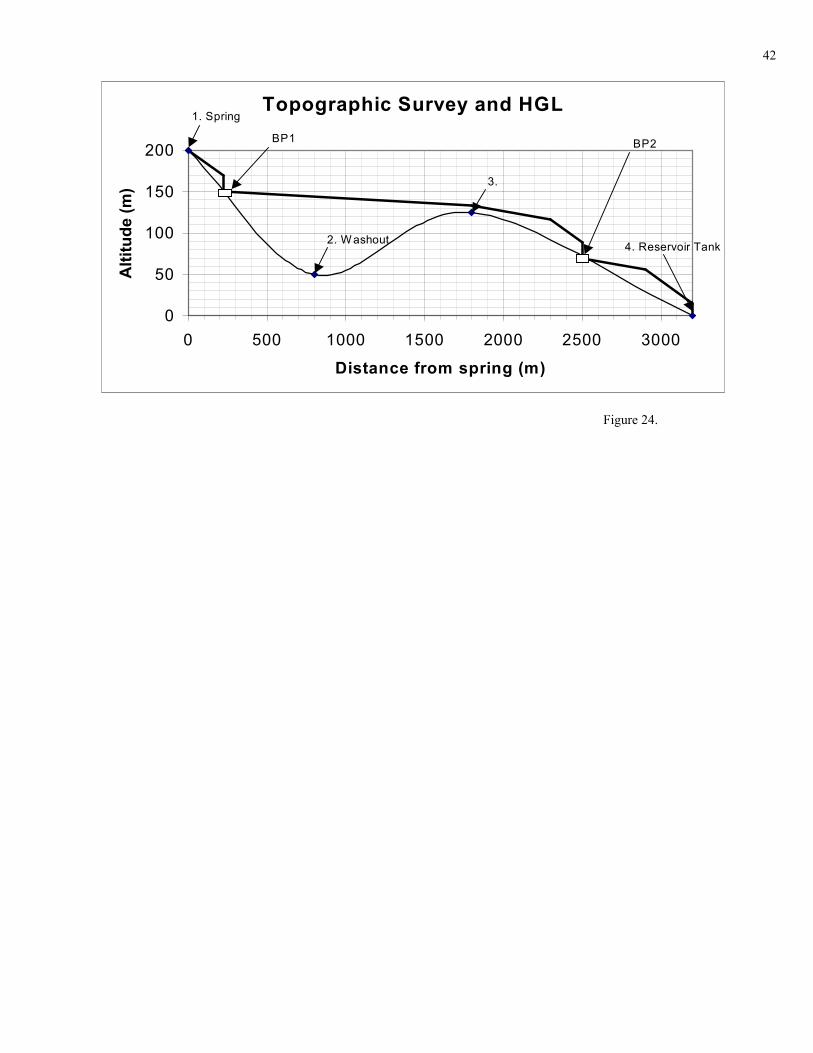
42
Topographic Survey and HGL
0
50
100
150
200
0 500 1000 1500 2000 2500 3000
Distance from spring (m)
Altitude (m)
1. Spring
2. Washout
3.
4. Reservoir Tank
BP1BP2
Figure 24.