flow nature's patterns
DESCRIPTION
Livro de Philip Ball (2009)TRANSCRIPT


Nature’s Patterns

This page intentionally left blank
Nature’sPatternsATapestry in Three Parts
Philip Ball
Nature’s Patterns is a trilogy composed ofShapes, Flow, and Branches
1

3Great Clarendon Street, Oxford OX2 6DP
Oxford University Press is a department of the University of Oxford.It furthers the University’s objective of excellence in research, scholarship,
and education by publishing worldwide in
Oxford New York
Auckland Cape Town Dar es Salaam Hong Kong KarachiKuala Lumpur Madrid Melbourne Mexico City Nairobi
New Delhi Shanghai Taipei Toronto
With offices in
Argentina Austria Brazil Chile Czech Republic France GreeceGuatemala Hungary Italy Japan Poland Portugal SingaporeSouth Korea Switzerland Thailand Turkey Ukraine Vietnam
Oxford is a registered trade mark of Oxford University Pressin the UK and in certain other countries
Published in the United Statesby Oxford University Press Inc., New York
# Philip Ball 2009
The moral rights of the author have been assertedDatabase right Oxford University Press (maker)
First published 2009
All rights reserved. No part of this publication may be reproduced,stored in a retrieval system, or transmitted, in any form or by any means,
without the prior permission in writing of Oxford University Press,or as expressly permitted by law, or under terms agreed with the appropriate
reprographics rights organization. Enquiries concerning reproductionoutside the scope of the above should be sent to the Rights Department,
Oxford University Press, at the address above
You must not circulate this book in any other binding or coverand you must impose the same condition on any acquirer
British Library Cataloguing in Publication Data
Data available
Library of Congress Cataloging in Publication Data
Data available
Typeset by SPI Publisher Services, Pondicherry, IndiaPrinted in Great Britainon acid-free paper byClays Ltd., St Ives plc
ISBN 978–0–19–923797–5
1 3 5 7 9 10 8 6 4 2
Flow
MOVEMENT creates pattern and form. Moving water arranges
itself into eddies, and sometimes places these in strict
array, where they become baroque and orderly conduits for
unceasing flow. The motions of air and water organize the skies, the
earth, and the oceans. The hidden logic of gases in turmoil paints great
spinning eyes on the outer planets. Out of the collisions of particles in
motion, desert dunes arise and hills become striped with sorted grains.
Give these grains the ability to respond to their neighbours—make
them fish, or birds, or buffalos—and there seems no end to the patterns
that may appear, each an extraordinary collaboration that no individual
has ordained or planned.

This page intentionally left blank

Contents
Preface and acknowledgements ix
1: The Man Who Loved Fluids 1
Leonardo’s Legacy
2: Patterns Downstream 21
Ordered Flows
3: On a Roll 50
How Convection Shapes the World
4: Riddle of the Dunes 77
When Grains Get Together
5: Follow Your Neighbour 124
Flocks, Swarms, and Crowds
6: Into the Maelstrom 164
The Trouble with Turbulence
Appendices 179
Bibliography 182
Index 187

This page intentionally left blank
Preface andacknowledgements
AFTER my 1999 book The Self-Made Tapestry: Pattern Formation
in Nature went out of print, I’d often be contacted by would-be
readers asking where they could get hold of a copy. That was
how I discovered that copies were changing hands in the used-book
market for considerably more than the original cover price. While that
was gratifying in its way, I would far rather see thematerial accessible to
anyone who wanted it. So I approached Latha Menon at Oxford Uni-
versity Press to ask about a reprinting. But Latha had something more
substantial in mind, and that is how this new trilogy came into being.
Quite rightly, Latha perceived that the original Tapestry was neither
conceived nor packaged to the best advantage of the material. I hope
this format does it more justice.
The suggestion of partitioning the material between three volumes
sounded challenging at first, but once I saw how it might be done,
I realized that this offered a structure that could bring more thematic
organization to the topic. Each volume is self-contained and does not
depend on one having read the others, although there is inevitably
some cross-referencing. Anyone who has seen The Self-Made Tapestry
will find some familiar things here, but also plenty that is new. In
adding that material, I have benefited from the great generosity of
many scientists who have given images, reprints and suggestions.
I am particularly grateful to Sean Carroll, Iain Couzin, and Andrea
Rinaldo for critical readings of some of the new text. Latha set me
more work than I’d perhaps anticipated, but I remain deeply indebted
to her for her vision of what these books might become, and her
encouragement in making that happen.
Philip Ball
London, October 2007

This page intentionally left blank
1The Man WhoLoved FluidsLeonardo’s Legacy
PERHAPS it is not so strange after all that the man who has come to
personify polyvalent virtuosity, defining the concept of the
Renaissance man and becoming a symbol for the unity of all
learning and creative endeavour, was something of an under-achiever.
That might seem an odd label to attach to Leonardo da Vinci, but the
fact is that he started very little and finished even less. His life was a
succession of plans made and never realized, of commissions refused
(or accepted and never honoured), of studies undertaken with such a
mixture of obsessive diligence and lack of system or objective that they
could offer little instruction to future generations. This was not because
Leonardo was a laggard; on the contrary, his ambitions often exceeded
his capacity to fulfil them.
Yet if Leonardo did not achieve as much as we feel he might have
done, that did not prevent his contemporaries from recognizing his
extraordinary genius. The Italian artist and writer Giorgio Vasari was
prone to eulogize all his subjects in his sixteenth-century Lives of the
Artists, but he seems to make a special effort for Leonardo:
In the normal course of events many men and women are born with various
remarkable qualities and talents; but occasionally, in a way that transcends
nature, a single person is marvellously endowed by heaven with beauty, grace,
and talent in such abundance that he leaves other men far behind, all his actions
seem inspired, and indeed everything he does clearly comes from God rather
than from human art. Everyone acknowledged that this was true of Leonardo da
Vinci, an artist of outstanding physical beauty who displayed infinite grace in
everything he did and who cultivated his genius so brilliantly that all problems
he studied he solved with ease.
What Vasari did not wish to admit is that such an embarrassment of
riches can be a burden rather than a blessing, and that it sometimes
takes duller men to see a project through to its end while geniuses can
only initiate them without cease. Leonardo’s devotion to the study of
nature and science could leave his artistic patrons frustrated. Isabella
d’Este, marchesa of Mantua, was told by an emissary whom she dis-
patched to Florence to commission a portrait from the great painter,
that ‘he is working hard at geometry and is very impatient of painting
. . . In short his mathematical experiments have so estranged him from
painting that he cannot bear to take up a brush.’
But Leonardo was apt when the mood was upon him to labour
without stint. His contemporary Matteo Bandello, a Piedmontese nov-
elist, saw him at work on his ill-fated Last Supper: ‘It was his habit often,
and I have frequently seen him, to go early in the morning and mount
upon the scaffolding . . . it was his habit, I say, from sunrise until dusk
never to lay down his brush, but, forgetful alike of eating and drinking,
to paint without intermission.’ And yet his genius demanded space for
reflection that he could ill afford. ‘At other times’, Bandello avers, ‘two,
three or four days would pass without his touching the fresco, but he
would remain before it for an hour or two at a time merely looking at it,
considering, examining the figures.’ ‘Oh dear, this man will never do
anything!’, Pope Leo X is said to have complained.
As his sketchbooks attest, lengthy and contemplative examination
was his forte. When Leonardo looked at something, he saw more than
other people. This was no idle gaze but an attempt to discern the very
soul of things, the deep and elusive forms of nature. In his studies of
anatomy, of animals and drapery, of plants and landscapes, and of
ripples and torrents of water, he shows us things that transcend the
naturalistic: shapes that we might not directly perceive ourselves but
that we suspect we would if we had Leonardo’s eyes.
We are accustomed to list Leonardo’s talents as though trying to assign
him to a university department: painter, sculptor, musician, anatomist,
military and civil engineer, inventor, physicist. But his notebooks mock
such distinctions. Rather, it seems that Leonardo was assailed by ques-
tions everywhere he looked, which he had hardly the opportunity or
inclination to arrange into a systematic course of study. Is the sound
of a blacksmith’s labours made with in the hammer or the anvil? Which
will fire farthest, gunpowder doubled in quantity or in quality? What
is the shape of corn tossed in a sieve? Are the tides caused by the
2 j NATURE’S PATTERNS: FLOW
Moon or the Sun, or by the ‘breathing of the Earth’? From where do
tears come, the heart or the brain? Why does a mirror exchange right
and left? Leonardo scribbles these memos to himself in his cryptic left-
handed script; sometimes he finds answers, but often the question is
left hanging. On his ‘to do’ list are items that boggle the mind with their
casual boldness: ‘Make glasses in order to see the moon large.’ It is no
wonder that Leonardo had no students and founded no school, for his
was an intensely personal enquiry into nature, one intended to satisfy
no one’s curiosity but his own.
We come no closer to understanding this quest, however, if we persist
in seeing Leonardo as an artist on the one hand and a scientist and
technologist on the other. The common response is to suggest that he
recognized no divisions between the two, and he is regularly invoked to
advertise the notion that both are complementary means of studying
and engaging with nature. This doesn’t quite hit the mark, however,
because it tacitly accepts that ‘art’ and ‘science’ had the same conno-
tations in Leonardo’s day as they do now. What Leonardo considered
arte was the business of making things. Paintings were made by arte,
but so were the apothecaries’ drugs and the weavers’ cloth. Until the
Renaissance there was nothing particularly admirable about art, or
at least about artists—patrons admired fine pictures, but the people
who made them were tradesmen paid to do a job, and manual workers
at that. Leonardo himself strove to raise the status of painting so that it
might rank among the ‘intellectual’ or liberal arts, such as geometry,
music, and astronomy. Although a formidable sculptor himself, he
argued his case by dismissing it as ‘less intellectual’: it is more endur-
ing, admittedly, ‘but excels in nothing else’. The academic and geomet-
ric character of treatises on painting at that time, most notably that of
the polymath Leon Battista Alberti, which can make painting seem less
amatter of inspiration than a process of drawing lines and plotting light
rays, derives partly from this agenda.
Scienza, in contrast, was knowledge—but not necessarily that obtained
by careful experiment and enquiry. Medieval scholastics had insisted
that knowledge was what appeared in the books of Euclid, Aristotle,
Ptolemy, and other ancient writers, and that the learned man was one
who had memorized these texts. The celebrated humanism of the
Renaissance did not challenge this idea but merely refreshed it, insisting
on returning to the original sources rather than relying on Arabic and
medieval glosses. In this regard, Leonardo was not a ‘scientist’, since he
THE MAN WHO LOVED FLUIDS j 3
was not well schooled—the humble son of a minor notary and a
peasant woman, he was defensive all his life about his poor Latin and
ignorance of Greek. He believed in the importance of scienza, certainly,
but for him this did not consist solely of book-learning. It was an active
pursuit, and demanded experiments, though Leonardo did not exactly
conduct them in the manner that a modern scientist would. For him,
true insight came from peering beneath the surface of things. That is
why his painstaking studies of nature, while appearing superficially
Aristotelian in their attention to particulars, actually have much more
of a Platonic spirit: they are an attempt to see what is really there, not
what appears to be. This is why he had to sit and stare for hours: not to
see things more sharply, but, as it were, to stop seeing, to transcend the
limitations of his eyes.
Leonardo regarded the task of the painter to be not naturalistic
mimicry, which shows only the surface contours and shallow glimmers
of the world, but the use of reason to shape his vision and distil from it a
kind of universal truth. ‘At this point’, Leonardo wrote of those who
would grow tired of his theoretical musings on the artist’s task, ‘the
opponent says that he does not want so much scienza, that practice is
enough for him in order to draw the things in nature. The answer to this
is that there is nothing that deceives usmore easily than our confidence
in our judgement, divorced from reasoning.’ This could have been
written by Plato himself, famously distrustful of the deceptions of
painters.
I hope you can start to appreciate why I have placed Leonardo centre
stage in introducing this volume of my survey of nature’s patterns. As
I explained in Book I, the desire to look through nature and find its
underlying forms and structures is what characterizes the approach of
some of the pioneers in the study of pattern formation, such as the
German biologist Ernst Haeckel and the Scottish zoologist D’Arcy Went-
worth Thompson. Haeckel was another gifted artist who firmly believed
that the natural world needs to be arranged, ordered, tidied, before its
forms and generative impulses can be properly perceived. Thompson
shared Leonardo’s conviction that the similarities of form and pattern we
see in verydifferent situations—forLeonardo itmight be the cascades of a
water spout and a woman’s hair—reveal a deep-seated relationship.
D’Arcy Thompson’s view of such correspondences is one we can still
accept in science today, based as it is on the idea that the same forces
are likely to be at play in both cases. Leonardo’s rationalization is more
4 j NATURE’S PATTERNS: FLOW

remote now from our experience, being rooted in the tradition of
Neoplatonism that saw these correspondences as a central feature of
nature’s divine architecture: as above, so below, as the reductive formu-
lation has it. When Leonardo calls rivers the blood of the Earth, and
comments on how their channels resemble the veins of the human
body, he is not engaging in some vaguemetaphor or visual pun; the two
are related because the Earth is indeed a kind of living body and can
therefore be expected to echo the structures of our own anatomy.
In this vision of a kind of hidden essence of nature, we can find the
true nexus of Leonardo’s ‘art’ and ‘science’. We tend to think of his art as
‘lifelike’, and Vasari made the same mistake. He praises the vase of
flowers that appears in one of Leonardo’s Madonnas for its ‘wonderful
realism’, but then goes on, I think inadvertently, to make a telling
remark by saying that the flowers ‘had on them dewdrops that looked
more convincing than the real thing’. Leonardo might have answered
that this was because he had indeed painted ‘the real thing’ and not
what his eyes had shown him. His work is not photographic but styl-
ized, synthetic, even abstract, and he admits openly that painting is a
work not of imitation but of invention: ‘a subtle inventione which with
philosophy and subtle speculation considers the natures of all forms’.
Leonardo ‘is thinking of art not simply in technical terms’, says art
historian Adrian Parr, ‘where the artist skillfully renders a form on the
canvas . . . Rather, he takes the relationship of nature to art onto a
deeper level, intending to express in his art ‘‘every kind of form pro-
duced in nature’’.’ For indeed, as the art historian Martin Kemp ex-
plains, ‘Leonardo saw nature as weaving an infinite variety of elusive
patterns on the basic warp and woof of mathematical perfection.’ And
so, without a doubt, did D’Arcy Thompson.
Leonardian flows
While most painters used technique to create a simulacrum of nature,
Leonardo felt that one could not imbue the picture with life until one
understood how nature does it. His sketches, then, are not exactly
studies but something between an experiment and a diagram—at-
tempts to intuit the forces at play (Fig. 1.1). ‘Leonardo’s use of swirling,
curving, revolving and wavy patterns, becomes a means of both inves-
tigating and entering into the rhythmicmovements of nature’, says Parr.
THE MAN WHO LOVED FLUIDS j 5

Other western artists have tried to capture the forms of movement and
flow, whether in the boiling vapours painted by J.M.W. Turner, the stop-
frame dynamism of Marcel Duchamp’s Nude Descending a Staircase
(1912) or the fragmented frenzy of the Italian Futurists. But these are
impressionistic, ad hoc and subjective efforts that lack Leonardo’s sci-
entific sense of pattern and order. Perhaps it is impossible truly to depict
the world in this way unless you are a Neoplatonist. When John Con-
stable declared in the early nineteenth century that ‘Painting is a science
and should be pursued as an inquiry into the laws of nature’, he had in
mind something far more mechanistic: that the painter should under-
stand howphysics andmeteorology create a play of light and shadow, so
that the paintings become convincing in an illusionistic sense.
Butwhile a Leonardianperspective is valuable for surveying all nature’s
patterns, I have made him the pinion for this volume on patterns
of motion, in fluids particularly, because there were few topics that
enthralled him (and I mean that in its original sense) more than this. Of
all the passions that he evinced, none seemsmore ardent than thewish to
understand water. One senses that he regards it as the central elemental
force: ‘water is the driver of Nature’, he says, ‘It is never at rest until it
unites with the sea . . . It is the expansion and humour of all vital bodies.
Without it nothing retains its form.’ It is no wonder, then, that one of
Leonardo’s most revealing and famous notebooks, known as the Codex
Fig. 1.1: A sketch of flowing water by Leonardo da Vinci.
6 j NATURE’S PATTERNS: FLOW
Leicester or Codex Hammer,* is mostly concerned with water. There was
hardly an aspect of water that Leonardo did not leave unexamined. He
wrote about sedimentation and erosion in rivers, and how they produce
meanders and sand ripples on the river bed (two patterns I consider
later). He discussed how water circulates on the Earth in what we now
call the hydrological cycle, evaporating from the seas and falling as rain
on tohighground.Heaskedwhy the sea is salty andwonderedwhy aman
can remain underwater only ‘for such a timeashe canhold his breath’. He
investigatedArchimedes spirals for liftingwater, aswell as suctionpumps
and water wheels. He drew astonishing ‘aerial’ pictures of river networks
(we’ll see them in Book III), and planned great works of hydraulic engin-
eering. In collaborationwithNiccoloMachiavelli, he drewupa scheme to
redirect the flow of the Arno River away from Pisa, thereby depriving the
city of its water supply and delivering it into the hands of the Florentines.
It seems that Leonardo did not become fascinated by water because
of his engineering activities; rather, according to art historian Arthur
Popham, the latter were a symptom of the former: ‘Something in the
movement of water, its swirls and eddies, corresponded to some deep-
seated twist in his nature.’ No aspect of water captured his interest
more than the eddies of a flowing stream. He wrote long lists of the
features of these vortices that he intended at some point to investigate:
Of eddies wide at the mouth and narrow at the base.
Of eddies very wide at the base and narrow above.
Of eddies of the shape of a column.
Of eddies formed between two masses of water that rub together.
And so on—pages and pages of optimistic plans, of experiments half-
started, of speculations and ideas, all described in such obsessive detail
that even Leonardo scholars have pronounced them virtually unread-
able. ‘He wants’, says the art historian Ernst Gombrich, ‘to classify
vortices as a zoologist classifies the species of animals.’
To judge from his sketches, Leonardo conducted a thorough, if hap-
hazard, experimental programme on the flow patterns of water, watch-
ing it pass down channels of different shapes, charting the chaos of
plunging waterfalls, and placing obstacles in the flow to see how they
generated new forms. His drawings of water surging around the sides of
a plate face-on to the flow show a delicately braided wake (Fig. 1.2a),
*The manuscript was acquired and published by Lord Leicester in Rome in the eighteenth
century, but was bought in 1980 by the American Maecenas Armand Hammer.
THE MAN WHO LOVED FLUIDS j 7
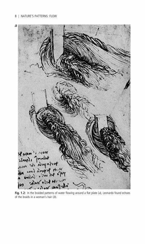
Fig. 1.2: In the braided patterns of water flowing around a flat plate (a), Leonardo found echoesof the braids in a woman’s hair (b).
8 j NATURE’S PATTERNS: FLOW

and the resemblance to the braided hair of a woman in a preparatory
study (Fig. 1.2b) is no coincidence, for as Leonardo said himself,
Observe the motion of the surface of the water which resembles that of hair,
which has two motions, of which one depends on the weight of the hair, the
other on the direction of the curls; thus the water forms eddying whirlpools, one
point of which is due to the impetus of the original current and the other to the
incidental motion and return flow.
Fig. 1.2: (Continued).
THE MAN WHO LOVED FLUIDS j 9
His self-portrait from 1512 shows his long hair and beard awash with
eddies.
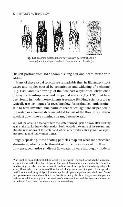
Many of these visual records are remarkably fine: he illustrates shock
waves and ripples caused by constriction and widening of a channel
(Fig. 1.3a), and his drawings of the flow past a cylindrical obstruction
display the teardrop wake and the paired vortices (Fig. 1.3b) that have
been found in modern experiments (see page 28). Fluid scientists today
typically use techniques for revealing flow-forms that Leonardo is often
said to have invented: fine particles that reflect light are suspended in
the water, or coloured dyes are added to part of the flow. ‘If you throw
sawdust down into a running stream’, Leonardo said,
you will be able to observe where the water turned upside down after striking
against the banks throws this sawdust back towards the centre of the stream, and
also the revolutions of the water and where other water either joins it or separ-
ates from it; and many other things.
Roughly speaking, these floating particles map out what are now called
streamlines, which can be thought of as the trajectories of the flow.* In
this sense, Leonardo’s studies of flow patterns were thoroughlymodern.
Fig. 1.3: Leonardo sketched shock waves caused by constrictions in achannel (a) and the shape of wakes in flow around an obstacle (b).
*A streamline has a technical definition: it is a line within the fluid for which the tangent at
any point shows the direction of flow at that point. Streamlines show not only ‘where the
fluid is going’ but also how fast: where streamlines are close together, the velocity is high. In
steady flows, where the pattern of flow doesn’t change over time, the path of a suspended
particle or the trajectory of dye injected at a point, the particle path or so-called streakline of
the dye trace out streamlines. But if the flow is unsteady, this is no longer true; the particle
paths or streaklines can give an impression of the streamlines, and the true streamlines can
be deduced from them, but they are not the same thing.
10 j NATURE’S PATTERNS: FLOW
But he had only his eyes and his memory to guide him in translating
from what he saw to what he drew; and as art historians know, that
translation occurs in a context of preconceived notions of style and
motif that condition what is depicted. When Leonardo compares a flow
to hair, he is struck initially by the resemblance, but then this corres-
pondence superimposes what he knows of the way hair falls on what he
sees in the stream of water. The result is, as Popham says, that although
[t]he cinematographic vision which could see, the prodigious memory which
could retain and the hand which could record these evanescent and intangible
formations are little short of miraculous . . . [t]hese drawings do not so much
convey the impression ofwater as of some exquisite submarine vegetable growth.
Was Leonardo able to do anything beyond recording what he per-
ceived? Did he elucidate the reasons why these marvellous patterns
are formed in water? If we have to admit that he did not really do that, it
is no disgrace, since that problem is one of the hardest of all in physical
science, and has still not been completely solved. On the whole the
flows that Leonardo was studying were turbulent, fast-moving and
unsteady in the extreme, so that they changed from one moment to
the next. If he could describe these flows only in pictures and words,
scientists could do no better than that until the twentieth century. And
what vivid descriptions he gave!—
The whole mass of water, in its breadth, depth and height, is full of innumerable
varieties of movements, as is shown on the surface of currents with a moderate
degree of turbulence, in which one sees continually gurglings and eddies with
various swirls formed by the more turbid water from the bottom as it rises to the
surface.
Leonardo made some discoveries that stand up today. His comment
that ‘water in straight rivers is swifter the farther it is from the shore, its
impediment’, for example, is an elegant description of what fluid scien-
tists call the velocity profile of flow in a channel, which is determined by
the way friction between the fluid and the channel wall brings the flow
there virtually to a standstill. Leonardo’s explanation of how river me-
anders are caused by shifting patterns of sedimentation and erosion by
the flow contain all the elements that today’s earth scientists recognize.
His legacy for our understanding of fluid flow patterns goes deeper
than this, however. As far as we can tell, Leonardo was the first Western
scientist to really make the case that this phenomenon deserves serious
study. And he showed that flowing water is not simply an unstructured
THE MAN WHO LOVED FLUIDS j 11
chaos but contains persistent forms that can be recognized, recorded,
analysed—forms, moreover, that are things of great beauty, of value to
the artist as well as the scientist.
Transcendental forms
All the same, Leonardo’s idiosyncratic, hermetic way of working meant
that no research programme stemmed from his achievements. No
scientist seems subsequently to have thought very much about fluid
flows until the Swiss mathematician Daniel Bernoulli began to investi-
gate them in the seventeenth century.*
Nor did Leonardo’s work on fluid motion have any artistic legacy: his
studies of flows as a play of patterns, forms, and streamlines leave no
trace in Western art. Artists looked instead for a stylized realism which
insisted that turbulent water be depicted as a play of glinting highlights
and surging foam: a style that is all surface, you might say. Just about
any dramatic seascape of the eighteenth or nineteenth centuries will
show this—George Morland’s The Wreckers (1791) is a good example
(Fig. 1.4).
A fluid style akin to Leonardo’s does not show up again in Western art
until the lively arabesques of the Art Nouveau movement of the late
nineteenth century (Fig. 1.5). These artists took their inspiration from
natural forms, such as the elegant curves and spirals of plant stems. As
I discussed in Book I, the delicate frond-like forms discovered at this
time in marine organisms and drawn with great panache and skill by
Ernst Haeckel became a significant influence on the German branch of
this movement, known as the Jugendstil—a two-way interaction that
probably conditioned the way Haeckel drew in the first place. In Eng-
land these trends produced something truly Leonardian in the works
of the illustrator Arthur Rackham, where the correspondences between
the waves and vortices of water, smoke, hair, and vegetation are par-
ticularly explicit (Fig. 1.6). But the use of vortical imagery here is
really nothing more than a style, valued for its decorative and allusive
qualities: there is no real sense that the artists are, like Leonardo,
*Rene Descartes made much of vortices, becoming convinced that the entire universe is
filled with an ethereal fluid that swirls at all scales. Their gyrating motions, he said, carry
along the heavenly bodies, explaining the circulations of the planets and stars. His theory,
however, does not seem to owe any inspiration to Leonardo’s work on eddies.
12 j NATURE’S PATTERNS: FLOW

simultaneously conducting an investigation into nature’s forms rather
than simply adapting them for aesthetic ends.
One of the sources of the bold lines and sinuous forms of Art Nouveau
is, however, more pertinent. In the mid-nineteenth century trade
opened up between Western Europe and the Far East, and Japanese
woodblock prints came into vogue among artist and collectors. Here
Western artists found a very differentway of depicting theworld—not as
naturalistic chiaroscuro but as a collage of flat, clearly delineated elem-
ents that disdains the rules of scientific optics andmakes no pretence of
photographic trompe l’oeil. To the Western eye these pictures are styl-
ized and schematic, but some artists could see that this was not mere
affectation, less still a simplification. What was being conveyed was the
essence of things, unobstructed by superficial incidentals.
It is as simplistic to generalize about Chinese and Japanese art as it is
about the art of the West—these traditions, too, have their different
periods and schools and philosophies. But it is fair to say that most
Chinese artists have attempted to imbue their works with Ch’i, the vital
Fig. 1.4: The Wreckers by George Morland shows the typical manner in which Western paintersdepicted flow as a play of light. (Image: Copyright Southampton City Art Gallery, Hampshire, UK/The Bridgeman Art Library.)
THE MAN WHO LOVED FLUIDS j 13
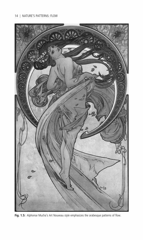
Fig. 1.5: Alphonse Mucha’s Art Nouveau style emphasizes the arabesque patterns of flow.
14 j NATURE’S PATTERNS: FLOW

energy of the universe, the Breath of the Tao. Ch’i is undefinable and
cannot be understood intellectually; the seventeenth-century painter’s
manual Chieh Tzu Yuan (The Mustard Seed Garden) explains that
‘Circulation of the Ch’i produces movement of life.’ So while the Taoist
conviction that there exists a fundamental simplicity beyond the super-
ficial shapes and forms of the world sounds Platonic, in fact it differs
Fig. 1.6: Arthur Rackham’s illustrations are Leonardian in their conflation of the eddies and tendrilsof fluid flow and the swirling of hair. (Image: Bridgeman Art Library.)
THE MAN WHO LOVED FLUIDS j 15

fundamentally. Unlike Plato’s notion of static, crystalline ideal forms,
the Tao is alive with spontaneity. It is precisely this spontaneity that the
Chinese classical artist would try to capture with movements of the
brush: ‘He who uses his mind and moves his brush without being
conscious of painting touches the secret of the art of painting’, said
the writer Chang Yen-yuan in the ninth century. In Chinese art every-
thing depends on the brushstrokes, the source and signifier of Ch’i.
No wonder, then, that among the stroke types classified by artistic
tradition was one called T’an wo ts’un: brushstrokes like an eddy or
whirlpool. No wonder either that the ancient painters of China would
say ‘Take five days to place water in a picture.’ What could be more
representative of the Tao than the currents of a river swirling around
rocks? But because the Tao is dynamic, an illusionistic rendering of a
frozen instant, like that in Western art, would be meaningless. Instead,
Chinese painters attempted to portray the inner life of flow, or what the
Fig. 1.7: In Chinese art, the flow of water is commonly represented as a series of linesapproximating the trajectories of floating particles, like the streamlines employed by fluiddynamicists. This is not a ‘realistic’ but a schematic depiction of flow. These images are takenfrom a painting instruction manual compiled in the late seventeenth century. (From M. M. Sze (ed.)(1977), The Mustard Seed Garden of Painting. Reprinted with permission of Princeton UniversityPress.)
16 j NATURE’S PATTERNS: FLOW
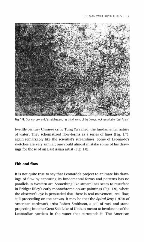
twelfth-century Chinese critic Tung Yu called ‘the fundamental nature
of water’. They schematized flow-forms as a series of lines (Fig. 1.7),
again remarkably like the scientist’s streamlines. Some of Leonardo’s
sketches are very similar; one could almost mistake some of his draw-
ings for those of an East Asian artist (Fig. 1.8).
Ebb and flow
It is not quite true to say that Leonardo’s project to animate his draw-
ings of flow by capturing its fundamental forms and patterns has no
parallels in Western art. Something like streamlines seem to resurface
in Bridget Riley’s early monochrome op-art paintings (Fig. 1.9), where
the observer’s eye is persuaded that there is real movement, real flow,
still proceeding on the canvas. It may be that the Spiral Jetty (1970) of
American earthwork artist Robert Smithson, a coil of rock and stone
projecting into the Great Salt Lake of Utah, is meant to invoke one of the
Leonardian vortices in the water that surrounds it. The American
Fig. 1.8: Some of Leonardo’s sketches, such as this drawing of the Deluge, look remarkably ‘East Asian’.
THE MAN WHO LOVED FLUIDS j 17
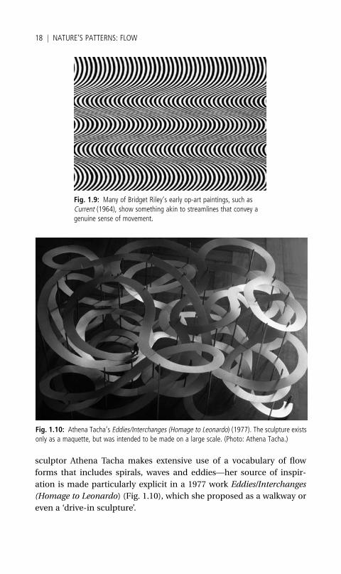
sculptor Athena Tacha makes extensive use of a vocabulary of flow
forms that includes spirals, waves and eddies—her source of inspir-
ation is made particularly explicit in a 1977 work Eddies/Interchanges
(Homage to Leonardo) (Fig. 1.10), which she proposed as a walkway or
even a ‘drive-in sculpture’.
Fig. 1.9: Many of Bridget Riley’s early op-art paintings, such asCurrent (1964), show something akin to streamlines that convey agenuine sense of movement.
Fig. 1.10: Athena Tacha’s Eddies/Interchanges (Homage to Leonardo) (1977). The sculpture existsonly as a maquette, but was intended to be made on a large scale. (Photo: Athena Tacha.)
18 j NATURE’S PATTERNS: FLOW
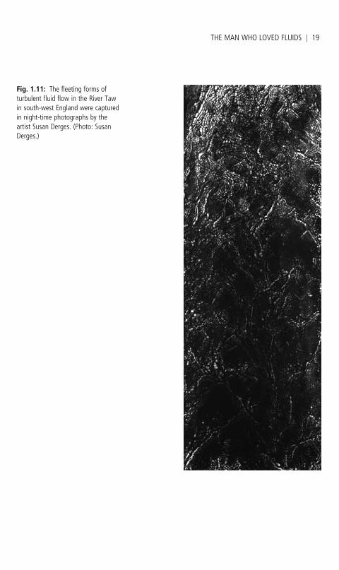
Fig. 1.11: The fleeting forms ofturbulent fluid flow in the River Tawin south-west England were capturedin night-time photographs by theartist Susan Derges. (Photo: SusanDerges.)
THE MAN WHO LOVED FLUIDS j 19
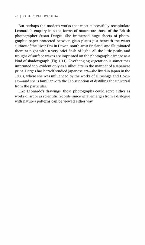
But perhaps the modern works that most successfully recapitulate
Leonardo’s enquiry into the forms of nature are those of the British
photographer Susan Derges. She immersed huge sheets of photo-
graphic paper protected between glass plates just beneath the water
surface of the River Taw in Devon, south-west England, and illuminated
them at night with a very brief flash of light. All the little peaks and
troughs of surface waves are imprinted on the photographic image as a
kind of shadowgraph (Fig. 1.11). Overhanging vegetation is sometimes
imprinted too, evident only as a silhouette in the manner of a Japanese
print. Derges has herself studied Japanese art—she lived in Japan in the
1980s, where she was influenced by the works of Hiroshige and Hoku-
sai—and she is familiar with the Taoist notion of distilling the universal
from the particular.
Like Leonardo’s drawings, these photographs could serve either as
works of art or as scientific records, since what emerges from a dialogue
with nature’s patterns can be viewed either way.
20 j NATURE’S PATTERNS: FLOW

2Patterns DownstreamOrder That Flows
THERE is nothing new in the idea that the transient forms of fluid
flow, frozen by the blink of a camera’s shutter, have artistic
appeal. As early as the 1870s, the British physicist Arthur
Worthington used high-speed photography to capture the hidden
beauty of splashes. He dropped pebbles into a trough of water and
discovered that the splash has an unguessed complexity and beauty
with a surprising degree of symmetry and order. Worthington worked
at the Royal Naval College in Devonport on the south-west coast of
England, where the study of impacts in water had decidedly unromantic
implications; but one senses that Worthington lost sight of the military
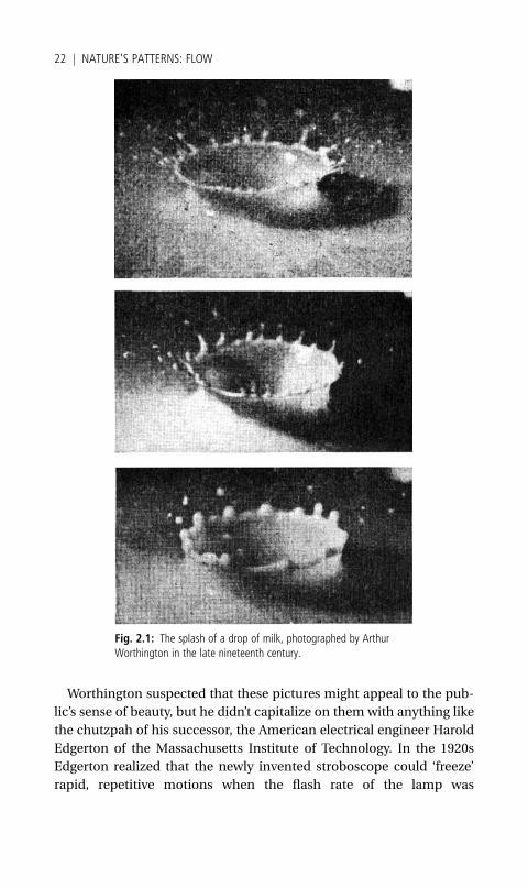
origins of his research as he fell under the allure of these images. A splash,
he found, erupts into a corona with a rim that breaks up into a series of
spikes, each of them releasing micro-droplets of their own (Fig. 2.1).
There is, he said, something seemingly ‘orderly and inevitable’ in these
forms, although he admitted that ‘it taxes the highest mathematical
powers’ to describe and explain them. In 1908 he collected his pictures
in a book called A Study of Splashes, which aimed to please the eye as
much as to inform the mind.
Worthington realized that the images were clearest if the liquid was
opaque, and so he used milk instead of water (the two are not equiva-
lent, for the higher viscosity of milk alters the shape of the splash). His
sequences of photos appear to represent a series of successive snap-
shots taken during the course of a single splash. But that is a forgivable
deception, for Worthington didn’t have a camera shutter able to open
and close at such a rate. Instead, each splash yielded a single image,
revealed in a flash of light from a spark that lasted for just a few
millionths of a second in a darkened room. To capture the sequence,
Worthington simply timed the spark at successively later instants in the
course of many splashes that he hoped were more or less identical.
Worthington suspected that these pictures might appeal to the pub-
lic’s sense of beauty, but he didn’t capitalize on them with anything like
the chutzpah of his successor, the American electrical engineer Harold
Edgerton of the Massachusetts Institute of Technology. In the 1920s
Edgerton realized that the newly invented stroboscope could ‘freeze’
rapid, repetitive motions when the flash rate of the lamp was
Fig. 2.1: The splash of a drop of milk, photographed by ArthurWorthington in the late nineteenth century.
22 j NATURE’S PATTERNS: FLOW
synchronized with the cycling rate of the movement. He developed a
stroboscopic photographic system that could take 3,000 frames
per second. His high-speed photographs became famous thanks to
Edgerton’s sense of eye-catching subject and composition: he took
split-second pictures of famous sportspeople and actors, and his iconic
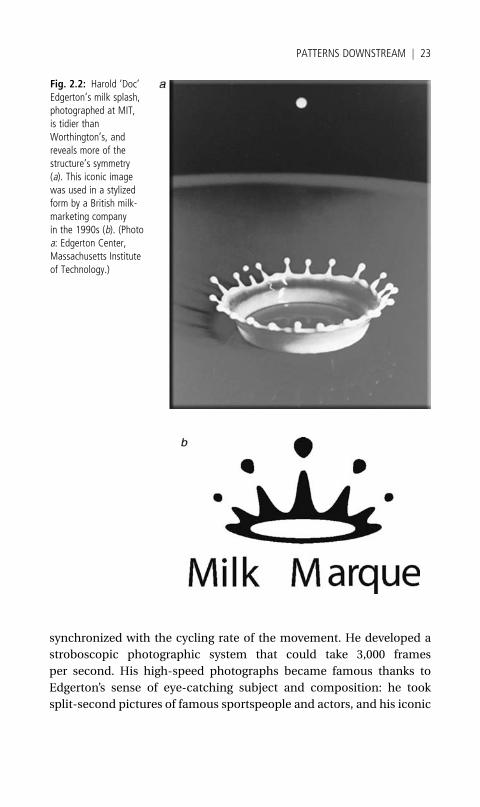
Fig. 2.2: Harold ‘Doc’Edgerton’s milk splash,photographed at MIT,is tidier thanWorthington’s, andreveals more of thestructure’s symmetry(a). This iconic imagewas used in a stylizedform by a British milk-marketing companyin the 1990s (b). (Photoa: Edgerton Center,Massachusetts Instituteof Technology.)
PATTERNS DOWNSTREAM j 23

‘Shooting the Apple’ pays homage to the legend of William Tell while
revealing the compelling destructiveness of a speeding bullet. In Edger-
ton’s quickfire lens, water running from the tap becomes petrified into
what appears to be a mound of solid glass. His book Flash (1939) was
unashamedly populist, a coffee-table collection of remarkable shots,
and his film Quicker ‘n a Wink (1940) won an Oscar the following year
for the best short film.
But probably the most memorable of Edgerton’s images was copied
straight fromWorthington: he filmedmilk droplets as they splash into a
smooth liquid surface. Edgerton’s drop is tidier, somehow more regular
and orderly, a true marvel of natural pattern (Fig. 2.2a): each prong of
the crown is more or less equidistant from its neighbours, and each of
them disgorges a single spherical globule.* This is the secret structure
of rainfall, reproduced countless times as raindrops fall into ponds and
puddles. Edgerton’s milk splash has become an icon of hidden order, as
much a work of art as a scientific study. More prosaically, the image was
adopted in the 1990s in stylized form by the British milk-marketing and
distribution company Milk Marque (Fig. 2.2b). D’Arcy Thompson was
captivated by these structures, too. In his classic book On Growth and
Form (1917) he compared Worthington’s fluted cup with its ‘scolloped’
and ‘sinuous’ edges to the forms a potter makes at amore leisurely pace
from wet clay. Edgerton’s photograph provided the front plate for the
1944 revised edition of the book, where it was as though Thompson
were saying ‘Look here, this is my subject. Here is the full mystery—the
quotidian, ubiquitous mystery—of pattern.’
To Thompson, who possessed a finely honed instinct for similarities
of pattern and shape in nature, these splash-forms were not just a
curiosity of fluid flow but a manifestation of a more general patterning
process that could be seen also in the shapes of soft-tissued living
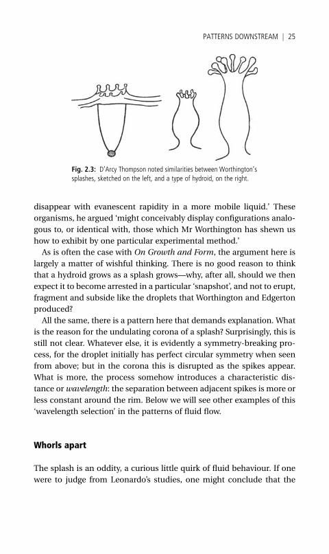
organisms. The bowl-like structure with its notched rim, he said, is
echoed in some species of hydroid, marine animals related to jellyfish
and sea anemones (Fig. 2.3). Of course, here the form is persistent,
not literally gone in a flash; yet ‘there is nothing’, Thompson said,
‘to prevent a slow and lasting manifestation, in a viscous medium
such as a protoplasmic organism, of phenomena which appear and
*You can watch Edgerton’s film of the splash online at <http://web.mit.edu/edgerton/
spotlight/Spotlight.html>. One can hardly view it now without noting the chilling resem-
blance to the aerial footage of the hydrogen-bomb tests of the 1950s—a documentary
technology to which Edgerton himself contributed.
24 j NATURE’S PATTERNS: FLOW
disappear with evanescent rapidity in a more mobile liquid.’ These
organisms, he argued ‘might conceivably display configurations analo-
gous to, or identical with, those which Mr Worthington has shewn us
how to exhibit by one particular experimental method.’
As is often the case with On Growth and Form, the argument here is
largely a matter of wishful thinking. There is no good reason to think
that a hydroid grows as a splash grows—why, after all, should we then
expect it to become arrested in a particular ‘snapshot’, and not to erupt,
fragment and subside like the droplets that Worthington and Edgerton
produced?
All the same, there is a pattern here that demands explanation. What
is the reason for the undulating corona of a splash? Surprisingly, this is
still not clear. Whatever else, it is evidently a symmetry-breaking pro-
cess, for the droplet initially has perfect circular symmetry when seen
from above; but in the corona this is disrupted as the spikes appear.
What is more, the process somehow introduces a characteristic dis-
tance orwavelength: the separation between adjacent spikes is more or
less constant around the rim. Below we will see other examples of this
‘wavelength selection’ in the patterns of fluid flow.
Whorls apart
The splash is an oddity, a curious little quirk of fluid behaviour. If one
were to judge from Leonardo’s studies, one might conclude that the
Fig. 2.3: D’Arcy Thompson noted similarities between Worthington’ssplashes, sketched on the left, and a type of hydroid, on the right.
PATTERNS DOWNSTREAM j 25
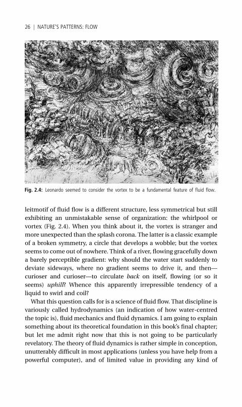
leitmotif of fluid flow is a different structure, less symmetrical but still
exhibiting an unmistakable sense of organization: the whirlpool or
vortex (Fig. 2.4). When you think about it, the vortex is stranger and
more unexpected than the splash corona. The latter is a classic example
of a broken symmetry, a circle that develops a wobble; but the vortex
seems to come out of nowhere. Think of a river, flowing gracefully down
a barely perceptible gradient: why should the water start suddenly to
deviate sideways, where no gradient seems to drive it, and then—
curioser and curioser—to circulate back on itself, flowing (or so it
seems) uphill? Whence this apparently irrepressible tendency of a
liquid to swirl and coil?
What this question calls for is a science of fluid flow. That discipline is
variously called hydrodynamics (an indication of how water-centred
the topic is), fluid mechanics and fluid dynamics. I am going to explain
something about its theoretical foundation in this book’s final chapter;
but let me admit right now that this is not going to be particularly
revelatory. The theory of fluid dynamics is rather simple in conception,
unutterably difficult in most applications (unless you have help from a
powerful computer), and of limited value in providing any kind of
Fig. 2.4: Leonardo seemed to consider the vortex to be a fundamental feature of fluid flow.
26 j NATURE’S PATTERNS: FLOW
intuitive picture of why fluids possess such an unnerving propensity for
pattern. It is, furthermore, a theory that is incomplete, for we still lack
any definitive understanding of the most extreme yet also the most
common state of fluid flow, which is turbulence. In everyday parlance,
‘turbulent’ is often a synonym for the disorganized, the chaotic, the
unpredictable—and while fluid turbulence does display these charac-
teristics to a greater or lesser degree, we can see from Leonardo’s
sketches (which invariably show turbulent flows) that there is a kernel
of orderliness in this chaos, most especially in the sense that turbulent
flow often retains the organized motions that spawn vortices.
For now, I shall describe fluid flow in the manner in which scientists
since Leonardo have been mostly compelled to do: by observing and
drawing pictures and writing not equations but prose. The French
mathematician Jean Leray, one of the great pioneers of fluid dynamics
in the twentieth century, formulated his ideas while gazing for long
hours at the problem in hand, standing on the Pont Neuf in Paris and
watching the Seine surge and ripple under the bridge. It is a testament
to Leray’s genius that this experience did not simply overwhelm him,
for, as much as you may plot graphs and make meticulous lab notes,
observing the flow of fluids can easily leave you with a sense of grasping
at the intangible.
Thinking about the problem as Leray did can at least help us to see
where we should start. Here is the Seine—not, by all accounts, the most
sanitary of rivers in the early part of the last century—streaming around
the piles of the Pont Neuf. The water parts as it flows each side of the
pillars, andthisdisturbance leaves itbillowingandturbulentdownstream.
To use the terminology we encountered in the first chapter, the stream-
lines become highly convoluted. How does that happen? Let’s back up a
little. If the water were not moving at all—if, instead of a river, the pillar
stands in a stagnant pond—then there is no pattern, since there is no
motionandnostreamlines.Wemustaskhowstill,uniformwaterbecomes
eddying flow. Let’s turn on the flow gradually and see what happens.
So here, then, is our idealized Seine: water flowing down a shallow
channel, which for simplicity we will assume to be flat-bottomed with
parallel, vertical sides. At slow flow rates, all the streamlines are straight
and parallel to the direction of flow—in other words, any little particle
that traces the flow, such as a leaf floating on the river surface, will
follow a simple, straight trajectory (Fig. 2.5a). At the edge of the ‘river’,
where the fluid rubs against the confining walls, we can imagine that
PATTERNS DOWNSTREAM j 27

something more complicated might happen, but actually this need not
alter the picture very much,* and in any event we can ignore that if we
make the river wide and focus on the middle, where the streamlines are
parallel and all of the fluid moves in synchrony, in the same direction at
the same speed. Flows like this in which the streamlines are parallel are
said to be laminar. The flow here is uniform throughout the water’s
depth (again, we can ignore the region where the water drags against
the river bottom), so we can depict it simply in terms of two-dimen-
sional streamlines.
Now it’s time to introduce the Pont Neuf, or, rather, the scientist’s
idealized version, which is a single cylindrical column standing in the
middle of the river (Fig. 2.5b). Clearly, some streamlines have to be
deflected around the cylinder. If the flow rate is very low, this can
happen smoothly: the streamlines part as they reach the cylinder and
converge again downstream to restore the laminar flow (Fig. 2.5b,c).
This creates a contained, lens-shaped region of disruption.
What happens if the flow rate increases? In the wake of the pillar, we
find that two little counter-circulating vortices, or eddies, appear
Fig. 2.5: Streamlines in the river. When fluid flow is slow andundisturbed, a floating particle follows a straight-line trajectory (a). Butif an obstacle is placed in the stream, the water must pass around it toeither side (b). At low flow speeds, the flow remains identical in allperpendicular layers, and so it can be represented in a single flat plane(c). Upstream, the diverted streamlines converge again. But at fasterspeeds, circulating vortices appear behind the obstacle (d), which growand elongate as the flow quickens its pace (e).
*A fluid will typically be slowed by friction where it touches the wall. If we think of it as being
divided into a series of parallel strips, the outermost stripmay be arrested entirely by friction.
The strip next to it is slowed down by the motionless layer, but not stopped entirely; and so
on with successive strips, each slowed a little less. So the velocity of the flow increases
smoothly from the walls, where it is zero, to the middle of the flow—just as Leonardo said.
28 j NATURE’S PATTERNS: FLOW
(Fig. 2.5d). The streamlines in the eddies are closed loops: there are
little pockets of fluid that have become detached from the main flow
and remain in place behind the pillar. A particle carried along in the
water would go round and round for ever if it got trapped in these
eddies. If the flow rate becomes still greater, the eddies grow and get
stretched out (Fig. 2.5e), but the flow outside of them remains laminar:
the streamlines eventually converge downstream and resume their
parallel paths.
It would be handy to have some way of measuring when these
changes happen. But we cannot simply say that, for example, the pair
of eddies appear at a flow speed of ten centimetres per second or
whatever, because in general this threshold also depends on factors
other than the fluid velocity, in particular the width of the pillar and the
viscosity of the liquid. However, one of the most profound and useful
discoveries of fluid dynamics is that flows can be described in terms of
‘universal’ measures that take all of these things into account. In this
case, let us assume that the flow is happening in a channel so wide that
the banks are very distant from the pillar and have no effect on the flow
there. Then we find that the flow velocity at which eddies first appear,
multiplied by the diameter of the pillar and divided by the viscosity of
the liquid, is always a constant, regardless of the type of liquid or the
dimensions of the pillar. This number has no units—they all cancel
out—but simply has a value of about four.
This is an example of a dimensionless number, one of the ‘universal
parameters’ that allows us to generalize about fluid flows without
having to take into account the specific details of our experimental
system. It is called the Reynolds number, after the British scientist
Osborne Reynolds who studied fluid flow in the nineteenth century.
It isn’t just a happy coincidence that this particular combination of
experimental parameters eliminates all units and gives a bare
number. Dimensionless numbers in fluid dynamics are in fact ratios
that express the relative contributions of the forces influencing the flow.
The Reynolds number (Re) measures the ratio of the forces driving the
flow (quantified by the flow velocity) to the forces retarding it by
viscous drag. In our experiment, the size of the pillar and the liquid
viscosity stay constant, and so Re increases in direct proportion to
the flow speed.
So then, at a Reynolds number of four, the flow pattern changes
abruptly with the appearance of the pair of vortices. The new pattern
PATTERNS DOWNSTREAM j 29
remains, albeit with increasingly elongated vortices, until Re reaches a
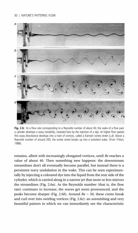
value of about 40. Then something new happens: the downstream
streamlines don’t all eventually become parallel, but instead there is a
persistent wavy undulation in the wake. This can be seen experimen-
tally by injecting a coloured dye into the liquid from the rear side of the
cylinder, which is carried along in a narrow jet that more or less mirrors
the streamlines (Fig. 2.6a). As the Reynolds number (that is, the flow
rate) continues to increase, the waves get more pronounced, and the
peaks become sharper (Fig. 2.6b). Around Re ¼ 50, these crests break
and curl over into swirling vortices (Fig. 2.6c): an astonishing and very
beautiful pattern in which we can immediately see the characteristic
Fig. 2.6: At a flow rate corresponding to a Reynolds number of about 40, the wake of a flow pasta cylinder develops a wavy instability, revealed here by the injection of a dye. At higher flow speedsthis wavy disturbance develops into a train of vortices, called a Karman vortex street (c,d). Above aReynolds number of around 200, the vortex street breaks up into a turbulent wake. (From Tritton,1988).
30 j NATURE’S PATTERNS: FLOW

traceries of Art Nouveau. In effect, the wake of the flow is continually
shedding eddies, first on one side and then on the other.
Although, as we have seen, structures rather like this can be seen in
Leonardo’s sketches, they do not seem to have been reported in a formal
scientific context until 1908, when the French physicist Henri Benard
published a paper called ‘Formation of rotation centres behind a mov-
ing obstacle’. But Benard’s work was not known to the German engineer
Ludwig Prantl when he made a study of cylinder wakes in 1911. Prantl
had a theory for such flows, and the theory said that the wake should
be smooth, rather like that in Fig. 2.5c. But when his doctoral student
Karl Hiemenz conducted experiments on this arrangement, he found
that the flow behind the obstacle underwent oscillations. Nonsense,
Prantl told him—clearly the cylinder isn’t smooth enough. Hiemenz
had it repolished, but found the same result. ‘Then your channel is not
perfectly symmetrical,’ Prantl told his hapless student, forcing him to
make further improvements.
At that time, a Hungarian engineer named Theodore von Karman
came to work in Prantl’s laboratory in Gottingen. He began to tease
Hiemenz, asking him each morning, ‘Herr Hiemenz, is the flow steady
now?’ Hiemenz would sigh glumly, ‘It always oscillates’. Eventually, von
Karman decided to see if he could understand what was going on.
A talented mathematician, he devised equations to describe the situ-
ation and found they predicted that vortices behind the cylinder could
be stable. As a result of this work, the trains of alternating vortices—
which, contrary to Prantl’s suspicions, are a real and fundamental
feature of the flow—are now known as Karman vortex streets.
Where do the vortices come from? They spring out of the layer of fluid
moving past the surface of the cylinder, which acquires a rotating
tendency called vorticity from the drag induced by the obstacle. This
process is highly coordinated between the ‘left’ and ‘right’ sides of the
pillar, so that as one vortex is being shed, that on the other side is in
the process of forming (Fig. 2.7). Vortex streets are common in nature.
They have been seen imprinted on clouds as air streams past some
obstacle such as a region of high pressure (Fig. 2.8). They are generated
in the wake of a bubble rising through water, pushing the bubble first to
one side and then the other as the vortices are shed; this explains why
the bubbles in champagne often follow a zigzag path as they rise. Vortex
shedding from the wingtips of flying insects helps them to defeat the
usual limitations of aerodynamics: in effect, the insects rotate their
PATTERNS DOWNSTREAM j 31

wings after a downstroke so that they receive a little push from the
circulating eddy this creates.
If the flow rate is increased still further, the vortices in the street begin
to lose their regularity, and the wake of the pillar seems to degenerate
into chaos. But in fact the orderliness of the flow comes and goes: an
observer stationed downstream would see more or less orderly vortex
streets pass by, interrupted now and then by bursts of disorderly tur-
bulence. Above Re ¼ 200, however, an observer a long distance down-
stream would note that the ordered vortex patterns seem to have
vanished for good. Even then, vortex streets persist close to the pillar
itself, but they get scrambled as they move downstream. At Re ¼ 400,
however, even this organization gets lost and the wake looks fully
turbulent. This is the typical situation for a river passing around the
piles of a bridge—rivers generally have a Reynolds number of more
than a million—and so Leray will have strained in vain to discern much
of a pattern in the murky Seine.
Unstable encounters
The transformation of a smooth, laminar flow into the wavy pattern
shown in Fig. 2.6a illustrates a common feature of pattern-forming
systems: the sudden onset of a wobble when the system is driven hard
enough. I discussed several such wave-like instabilities in Book I, from
the fragmentation of columns of liquid to the appearance of oscillations
in a chemical reaction. What creates the wave in this instance?
Fig. 2.7: The Karman vortex street arises from ‘eddy shedding’.Circulating vortices behind the obstacle are shed from alternate sidesand borne along in the wake. Here one eddy is in the process offorming just after that on the opposite side has been shed. (FromTritton, 1988.)
32 j NATURE’S PATTERNS: FLOW
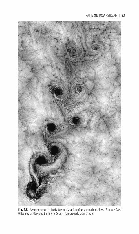
Fig. 2.8: A vortex street in clouds due to disruption of an atmospheric flow. (Photo: NOAA/University of Maryland Baltimore County, Atmospheric Lidar Group.)
PATTERNS DOWNSTREAM j 33
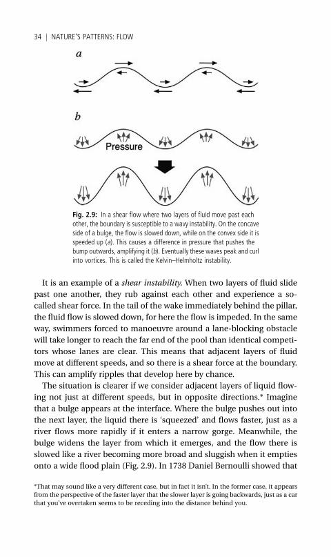
It is an example of a shear instability. When two layers of fluid slide
past one another, they rub against each other and experience a so-
called shear force. In the tail of the wake immediately behind the pillar,
the fluid flow is slowed down, for here the flow is impeded. In the same
way, swimmers forced to manoeuvre around a lane-blocking obstacle
will take longer to reach the far end of the pool than identical competi-
tors whose lanes are clear. This means that adjacent layers of fluid
move at different speeds, and so there is a shear force at the boundary.
This can amplify ripples that develop here by chance.
The situation is clearer if we consider adjacent layers of liquid flow-
ing not just at different speeds, but in opposite directions.* Imagine
that a bulge appears at the interface. Where the bulge pushes out into
the next layer, the liquid there is ‘squeezed’ and flows faster, just as a
river flows more rapidly if it enters a narrow gorge. Meanwhile, the
bulge widens the layer from which it emerges, and the flow there is
slowed like a river becoming more broad and sluggish when it empties
onto a wide flood plain (Fig. 2.9). In 1738 Daniel Bernoulli showed that
*That may sound like a very different case, but in fact it isn’t. In the former case, it appears
from the perspective of the faster layer that the slower layer is going backwards, just as a car
that you’ve overtaken seems to be receding into the distance behind you.
Fig. 2.9: In a shear flow where two layers of fluid move past eachother, the boundary is susceptible to a wavy instability. On the concaveside of a bulge, the flow is slowed down, while on the convex side it isspeeded up (a). This causes a difference in pressure that pushes thebump outwards, amplifying it (b). Eventually these waves peak and curlinto vortices. This is called the Kelvin–Helmholtz instability.
34 j NATURE’S PATTERNS: FLOW
the pressure exerted by a liquid lateral to the direction of flow decreases
as the flow gets faster. This explains why the shower curtain always
sticks to you: as the jet of water moves the layer of air between your skin
and the curtain, the pressure there falls and the curtain gets pushed
inwards by the air pressure on the other side.
This means that there is low pressure on the convex side of the bulge
and high pressure on the concave side, so the bulge gets pushed
outwards and accentuated. In other words, there is positive feedback:
the more the bulge grows, the greater its tendency to grow further. This
seems to imply that any bulge at the boundary of a shear flow will be
self-amplifying. But in practice, the viscosity of the liquid (a measure of
its resistance to flow) damps out the instability until the shear force
(here depending on the relative velocity of the two layers) exceeds some
critical threshold. What is more, the self-amplification is greatest at a
particular wavelength of undulation, and so this wavy pattern gets
‘selected’ from all the others. The result is that the shear flow develops
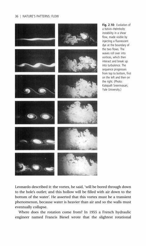
a regular series of waves (Fig. 2.10).
This shear instability was studied in the nineteenth century by two of
its greatest physicists, Lord Kelvin and Hermann von Helmholtz, and it
is now known as the Kelvin–Helmholtz instability. The waves become
sharply peaked as the structure evolves, and are then pulled over into
curling breakers, producing a series of vortices.* Kelvin–Helmholtz in-
stabilities are another of the patterning mechanisms that operate in the
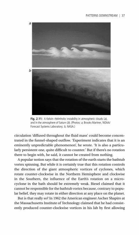
atmosphere, appearing for example in clouds or air layers (Fig. 2.11a).
I have seen them myself in the sky above London. NASA’s Cassini
spacecraft captured a particularly striking example in the atmosphere
of Saturn, where bands of gases move past one another (Fig. 2.11b).
Plugholes and whirlpools
Shear instabilities can thus stir fluids into whirlpools. These flow-forms
range in scale from the mundane spiralling of bath water around the
plughole to the terrifying gyrations of tornadoes and hurricanes
(Fig. 2.12). The bathtub vortex puzzled scientists for centuries.
*I must stress that this is not how the vortices of a Karman vortex street are made, however.
The waviness in Fig. 2.6 is indeed a shear instability, but the vortices grow from the edge of
the pillar, not from the peaks of the downstream waves.
PATTERNS DOWNSTREAM j 35
Leonardo described it: the vortex, he said, ‘will be bored through down
to the hole’s outlet; and this hollow will be filled with air down to the
bottom of the water’. He asserted that this vortex must be a transient
phenomenon, because water is heavier than air and so the walls must
eventually collapse.
Where does the rotation come from? In 1955 a French hydraulic
engineer named Francis Biesel wrote that the slightest rotational
Fig. 2.10: Evolution ofa Kelvin–Helmholtzinstability in a shearflow, made visible byinjecting a fluorescentdye at the boundary ofthe two flows. Thewaves roll over intovortices, which theninteract and break upinto turbulence. Thesequence progressesfrom top to bottom, firston the left and then onthe right. (Photo:Katepalli Sreenivasan,Yale University.)
36 j NATURE’S PATTERNS: FLOW
circulation ‘diffused throughout the fluid mass’ could become concen-
trated in the funnel-shaped outflow. ‘Experiment indicates that it is an
eminently unpredictable phenomenon’, he wrote. ‘It is also a particu-
larly persistent one, quite difficult to counter.’ But if there’s no rotation
there to begin with, he said, it cannot be created from nothing.
A popular notion says that the rotation of the earth starts the bathtub
vortex spinning. But while it is certainly true that this rotation controls
the direction of the giant atmospheric vortices of cyclones, which
rotate counter-clockwise in the Northern Hemisphere and clockwise
in the Southern, the influence of the Earth’s rotation on a micro-
cyclone in the bath should be extremely weak. Biesel claimed that it
cannot be responsible for the bathtub vortex because, contrary to popu-
lar belief, they may rotate in either direction at any place on the planet.
But is that really so? In 1962 the American engineer Ascher Shapiro at
the Massachusetts Institute of Technology claimed that he had consist-
ently produced counter-clockwise vortices in his lab by first allowing
Fig. 2.11: A Kelvin–Helmholtz instability in atmospheric clouds (a),and in the atmosphere of Saturn (b). (Photos: a, Brooks Martner, NOAA/Forecast Systems Laboratory; b, NASA.)
PATTERNS DOWNSTREAM j 37
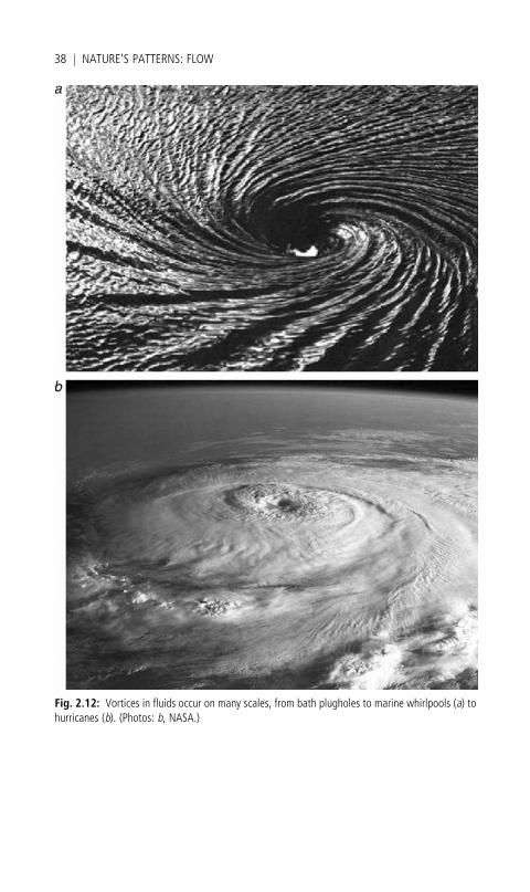
Fig. 2.12: Vortices in fluids occur on many scales, from bath plugholes to marine whirlpools (a) tohurricanes (b). (Photos: b, NASA.)
38 j NATURE’S PATTERNS: FLOW
the water to settle for 24 hours, dissipating any residual rotational
motion, before pulling the plug. The claim sparked controversy: later
researchers said that the experiment was extremely sensitive to the
precise conditions in which it was conducted. The dispute has never
quite been resolved.
We do know, however, why a small initial rotation of the liquid de-
velops into a robust vortex. This is due to themovement of thewater as it
converges on the outlet. In theory this convergence can be completely
symmetrical: water moves inwards to the plughole from all directions.
But the slightest departure from that symmetrical situation, which
could happen at random, may be amplified because of the way fluid
flow operates. Flow may be transmitted from one region of fluid to
another because of friction. This is why you can stir your coffee by
blowing across the top, and why ocean surface currents are awakened
by the wind: one flow drives another. A small amount of rotation excites
more, and then more again . . . To sustain this process, however, the
nascent vortex needs to be constantly supplied with momentum, just
as you need to keep pushing a child on a swing to keep them moving.
This momentum is provided by the inflow of water towards the plug-
hole: in effect, the momentum of movement in a straight line is con-
verted to the momentum of rotation.
The plughole vortex is an example of spontaneous symmetry-break-
ing: a radially converging flow, with circular symmetry, develops into a
flow with an asymmetric twist, either clockwise or counter-clockwise
depending on the nature of the imperceptible push that gets the rota-
tion under way. Setting aside Shapiro’s ambiguous experiments, this
initial kick seems to happen at random, and there is no telling which
way the bathtub vortex will spin.
Marine whirlpools have spawned many legends, from Charybdis of
the Odyessy to the Maelstrom of Nordic tales. Centrifugal forces act on
the spinning water to push the surface of a whirlpool into an inverted
bell-shape, which is embellished by ripples excited near the centre to
produce the familiar corkscrew appearance (Fig. 2.12a). Some of these
structures, like the Maelstrom and the vortex at St Malo in the English
Channel, are caused by tidal flows near to shore, which is precisely why
they are so hazardous to seamen. Poe’s terrifying account of a Norwe-
gian fisherman’s Descent into the Maelstrom (‘the boat appeared to be
hanging, as if by magic, midway down, upon the interior surface of a
funnel vast in circumference, prodigious in depth’) is uncannily
PATTERNS DOWNSTREAM j 39

accurate not just in a pictorial sense but in terms of the underlying fluid
dynamics, suggesting that perhaps Poe took his information from a
real-life encounter.
Vortices appear not just in sluggishly flowing fluids but also in fully
turbulent ones. Although such flows seem disorderly and unpredict-
able, nevertheless the fluids retain a propensity to organize themselves
into these distinct, coherent structures. This was demonstrated by
Dutch physicists GertJan van Heijst and Jan-Bert Flor at the University
of Utrecht, who showed that a kind of two-headed vortex (the technical
term is ‘dipolar’) can emerge from a turbulent jet. They fired a jet of
coloured dye into water whose saltiness increased with depth. This
gradient in saltiness meant that the water got denser as it got deeper,
which suppressed up-and-down currents in the fluid, making the flow
essentially two-dimensional: each horizontal layer flowed in the same
way. The initially disordered flow in the head of the jet gradually
arranged itself into two counter-rotating lobes (Fig. 2.13). And to
show just how robust these dipolar vortices are, van Heijst and Flor
fired two of them at each other from opposite directions, so that they
Fig. 2.13: A turbulent jet injected into a stratified fluid (in which adensity gradient keeps the flow essentially two-dimensional) organizesitself into a coherent structure, the dipolar vortex. (Photos: GertJan vanHeijst and Jan-Bert Flor, University of Utrecht.)
40 j NATURE’S PATTERNS: FLOW
collided head on. This might be expected to generate a turbulent frenzy,
but instead the vortices displayed a slippery resilience that somehow
makes you think of egg yolks. As they collided, they simply paired up
with their counterpart in the other jet and, without mixing, set off in
new directions (Plate 1).
The giant’s eye
One of the most celebrated and dramatic of the vortices found in a
natural turbulent flow has been gyrating for over a century. Jupiter’s
Great Red Spot is a maelstrom to cap them all: as wide as the Earth and
three times as long, it is a storm in Jupiter’s southern hemisphere in
which the winds reach speeds of around 350 miles an hour (Plate 2). It
is often said that the Red Spot was first observed in the seventeenth
century by Robert Hooke in England and by Giovanni Domenico Cas-
sini in Italy. But it is not clear that either of these scientists saw today’s
Red Spot. Cassini’s spot, which he reported in 1665, was subsequently
observed until 1713, but after that the records fall silent until the
sighting of the present Red Spot in 1830. Vortices like this do come
and go on Jupiter—three white spots to the south of the Great Red Spot
appeared in 1938 and persisted until 1998, when they merged into a
single spot.* The Great Red Spot itself seems to be diminishing since its
observation in the nineteenth century, and it is very likely that one day
Jupiter’s eye will close again. How do these structures arise, and how
can they for so long defy the disruptive pull of turbulence?
The colours of Jupiter’s cloudy upper atmosphere are caused by its
complex chemical make-up: a mixture of hydrogen and helium with
clouds of water, ammonia, and other compounds. All this is stirred by
the planet’s rotation into a swirling brew, which is patterned even
before we start to consider the spots. The Jovian atmosphere is divided
into a series of bands marked out in different colours (Plate 3). Each
band is a ‘zonal jet’, a stream that flows around lines of latitude either in
the same or the opposite direction to the planet’s rotation. The Earth
has zonal jets, too: the eastward current of the trade winds in the
tropics, and the westward current of the jet stream at higher latitudes.
*In 2005–6 this turned red, presumably because its increased strength dredged up some red
material from deeper in the atmosphere. It has been dubbed Red Spot Junior.
PATTERNS DOWNSTREAM j 41

On Jupiter, both hemispheres have several zonal jets travelling to the
east and west. The origin of these bands is still disputed, but they may
be the product of small-scale eddies pulled and blended into latitudinal
jets by the planet’s rotation.
Peter Olson and Jean-Baptiste Manneville have shown that a similar
banded structure can arise from convection in a laboratory model of
Jupiter’s atmosphere. They used water to mimic the fluid atmosphere
(since it has a similar density), trapped between two concentric spheres
25 and 30 centimetres across. The inner sphere was chilled by filling it
with cold antifreeze; the outer sphere was of clear plastic, so that the
flow pattern could be seen. The researchers simulated the effect of the
planet’s gravity by spinning both spheres to create a centrifugal force,
and added a fluorescent dye to the water so that the flow pattern could
be seen under ultraviolet light. They saw zonal bands appear around
their model planet because of convective motions. We will see in the
next chapter how such rolls and stripes are a common feature of
convection patterns.
The spot features in Jupiter’s atmosphere are formed at the boundary
of two zonal jets, where the movement of gases in opposite directions
creates an intense shear flow. The Great Red Spot circulates like a ball
bearingbetween theflowsaboveandbelow (Fig. 2.14). There is nowreason
to think that a single big vortex like this may be a very general feature
of this kind of turbulent flow. Philip Marcus from the University of Cali-
fornia at Berkeley has carried out numerical calculations of the flow in a
Fig. 2.14: Jupiter’s Great Red Spot circulates between oppositelydirected zonal jets that encircle the planet.
42 j NATURE’S PATTERNS: FLOW
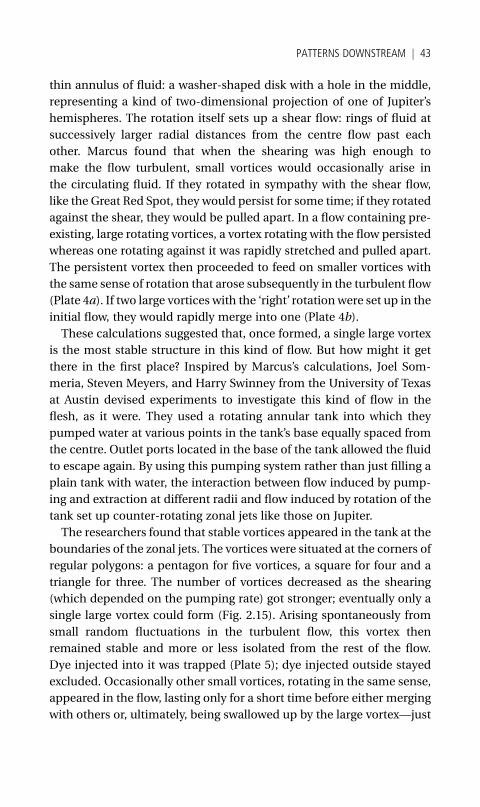
thin annulus of fluid: a washer-shaped disk with a hole in the middle,
representing a kind of two-dimensional projection of one of Jupiter’s
hemispheres. The rotation itself sets up a shear flow: rings of fluid at
successively larger radial distances from the centre flow past each
other. Marcus found that when the shearing was high enough to
make the flow turbulent, small vortices would occasionally arise in
the circulating fluid. If they rotated in sympathy with the shear flow,
like the Great Red Spot, they would persist for some time; if they rotated
against the shear, they would be pulled apart. In a flow containing pre-
existing, large rotating vortices, a vortex rotating with the flow persisted
whereas one rotating against it was rapidly stretched and pulled apart.
The persistent vortex then proceeded to feed on smaller vortices with
the same sense of rotation that arose subsequently in the turbulent flow
(Plate 4a). If two large vortices with the ‘right’ rotation were set up in the
initial flow, they would rapidly merge into one (Plate 4b).
These calculations suggested that, once formed, a single large vortex
is the most stable structure in this kind of flow. But how might it get
there in the first place? Inspired by Marcus’s calculations, Joel Som-
meria, Steven Meyers, and Harry Swinney from the University of Texas
at Austin devised experiments to investigate this kind of flow in the
flesh, as it were. They used a rotating annular tank into which they
pumped water at various points in the tank’s base equally spaced from
the centre. Outlet ports located in the base of the tank allowed the fluid
to escape again. By using this pumping system rather than just filling a
plain tank with water, the interaction between flow induced by pump-
ing and extraction at different radii and flow induced by rotation of the
tank set up counter-rotating zonal jets like those on Jupiter.
The researchers found that stable vortices appeared in the tank at the
boundaries of the zonal jets. The vortices were situated at the corners of
regular polygons: a pentagon for five vortices, a square for four and a
triangle for three. The number of vortices decreased as the shearing
(which depended on the pumping rate) got stronger; eventually only a
single large vortex could form (Fig. 2.15). Arising spontaneously from
small random fluctuations in the turbulent flow, this vortex then
remained stable and more or less isolated from the rest of the flow.
Dye injected into it was trapped (Plate 5); dye injected outside stayed
excluded. Occasionally other small vortices, rotating in the same sense,
appeared in the flow, lasting only for a short time before either merging
with others or, ultimately, being swallowed up by the large vortex—just
PATTERNS DOWNSTREAM j 43
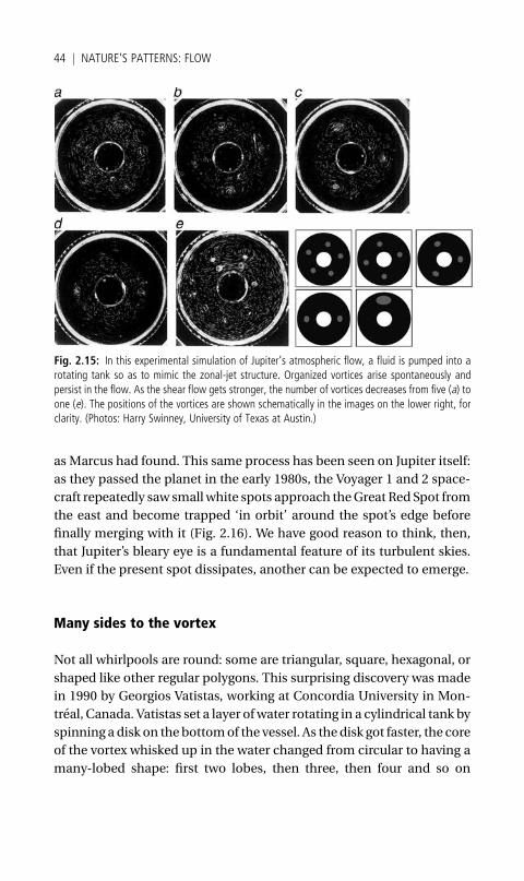
as Marcus had found. This same process has been seen on Jupiter itself:
as they passed the planet in the early 1980s, the Voyager 1 and 2 space-
craft repeatedly saw smallwhite spots approach theGreat Red Spot from
the east and become trapped ‘in orbit’ around the spot’s edge before
finally merging with it (Fig. 2.16). We have good reason to think, then,
that Jupiter’s bleary eye is a fundamental feature of its turbulent skies.
Even if the present spot dissipates, another can be expected to emerge.
Many sides to the vortex
Not all whirlpools are round: some are triangular, square, hexagonal, or
shaped like other regular polygons. This surprising discovery was made
in 1990 by Georgios Vatistas, working at Concordia University in Mon-
treal, Canada. Vatistas set a layer ofwater rotating in a cylindrical tank by
spinning a disk on thebottomof the vessel. As thedisk got faster, the core
of the vortex whisked up in the water changed from circular to having a
many-lobed shape: first two lobes, then three, then four and so on
Fig. 2.15: In this experimental simulation of Jupiter’s atmospheric flow, a fluid is pumped into arotating tank so as to mimic the zonal-jet structure. Organized vortices arise spontaneously andpersist in the flow. As the shear flow gets stronger, the number of vortices decreases from five (a) toone (e). The positions of the vortices are shown schematically in the images on the lower right, forclarity. (Photos: Harry Swinney, University of Texas at Austin.)
44 j NATURE’S PATTERNS: FLOW
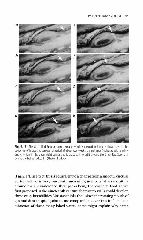
(Fig. 2.17). In effect, this is equivalent to a change froma smooth, circular
vortex wall to a wavy one, with increasing numbers of waves fitting
around the circumference, their peaks being the ‘corners’. Lord Kelvin
first proposed in the nineteenth century that vortex walls could develop
these wavy instabilities. Vatistas thinks that, since the rotating clouds of
gas and dust in spiral galaxies are comparable to vortices in fluids, the
existence of these many-lobed vortex cores might explain why some
Fig. 2.16: The Great Red Spot consumes smaller vortices created in Jupiter’s shear flow. In thissequence of images, taken over a period of about two weeks, a small spot (indicated with a whitearrow) enters in the upper right corner and is dragged into orbit around the Great Red Spot untileventually being sucked in. (Photos: NASA.)
PATTERNS DOWNSTREAM j 45
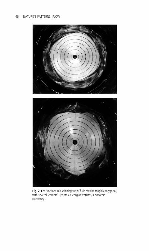
Fig. 2.17: Vortices in a spinning tub of fluid may be roughly polygonal,with several ‘corners’. (Photos: Georgios Vatistas, ConcordiaUniversity.)
46 j NATURE’S PATTERNS: FLOW
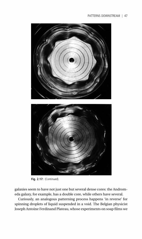
galaxies seem to have not just one but several dense cores: the Androm-
eda galaxy, for example, has a double core, while others have several.
Curiously, an analogous patterning process happens ‘in reverse’ for
spinning droplets of liquid suspended in a void. The Belgian physicist
Joseph Antoine Ferdinand Plateau, whose experiments on soap filmswe
Fig. 2.17: (Continued).
PATTERNS DOWNSTREAM j 47

encountered in Book I, discovered in the 1860s that a spinning droplet
becomes deformed into a two-lobed ‘peanut’ shape when it rotates fast
enough. Plateau too was interested in astrophysical implications—
he wondered whether his droplet might mimic rapidly spinning stars
or planets. Richard Hill and Laurence Eaves of the University of Not-
tingham in England have performed a more sophisticated version of
Plateau’s experiment (which used droplets of oil suspended in a water-
alcohol mixture) by using strong magnetic fields to levitate droplets of
water as big as grapes (14 mm in diameter). They spun these drops by
passing an electric current through them to create a sort of ‘liquid
motor’. Hill and Eaves saw the droplets develop three, four and five
lobes—crudely speaking, becoming triangular, square and pen-
tagonal—as the spinning got faster. It seems possible that some fast-
spinning asteroid-like objects in the so-called Kuiper belt beyond the
orbit of Pluto, some of which are piles of rubble held together loosely by
gravity, might also have three lobes. For both vortices and droplets,
then, rotation can break the symmetry, transforming an initially circular
object into one with ‘corners’.
Fig. 2.18: The ‘square’ eyewall of Hurricane Ivan.
48 j NATURE’S PATTERNS: FLOW
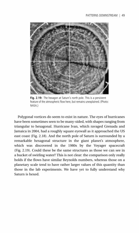
Polygonal vortices do seem to exist in nature. The eyes of hurricanes
have been sometimes seen to bemany-sided, with shapes ranging from
triangular to hexagonal. Hurricane Ivan, which ravaged Grenada and
Jamaica in 2004, had a roughly square eyewall as it approached the US
east coast (Fig. 2.18). And the north pole of Saturn is surrounded by a
remarkable hexagonal structure in the giant planet’s atmosphere,
which was discovered in the 1980s by the Voyager spacecraft
(Fig. 2.19). Could these be the same structures as those we can see in
a bucket of swirling water? This is not clear: the comparison only really
holds if the flows have similar Reynolds numbers, whereas those on a
planetary scale tend to have rather larger values of this quantity than
those in the lab experiments. We have yet to fully understand why
Saturn is hexed.
Fig. 2.19: The hexagon at Saturn’s north pole. This is a persistentfeature of the atmospheric flow here, but remains unexplained. (Photo:NASA.)
PATTERNS DOWNSTREAM j 49
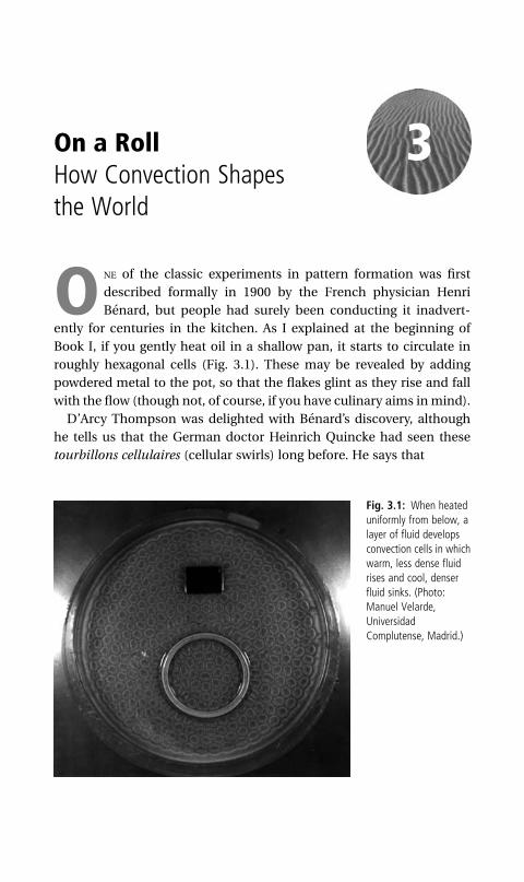
3On a RollHow Convection Shapesthe World
ONE of the classic experiments in pattern formation was first
described formally in 1900 by the French physician Henri
Benard, but people had surely been conducting it inadvert-
ently for centuries in the kitchen. As I explained at the beginning of
Book I, if you gently heat oil in a shallow pan, it starts to circulate in
roughly hexagonal cells (Fig. 3.1). These may be revealed by adding
powdered metal to the pot, so that the flakes glint as they rise and fall
with the flow (though not, of course, if you have culinary aims inmind).
D’Arcy Thompson was delighted with Benard’s discovery, although
he tells us that the German doctor Heinrich Quincke had seen these
tourbillons cellulaires (cellular swirls) long before. He says that
Fig. 3.1: When heateduniformly from below, alayer of fluid developsconvection cells in whichwarm, less dense fluidrises and cool, denserfluid sinks. (Photo:Manuel Velarde,UniversidadComplutense, Madrid.)
The liquid is under peculiar conditions of instability, for the least fortuitous excess
of heat here or there would suffice to start a current, and we should expect
the system to be highly unstable and unsymmetrical . . . [but] whether we start
with a liquid inmotion or at rest, symmetry and uniformity are ultimately attained.
The cells draw towards uniformity, but four, five or seven-sided cells are still to be
found among the prevailing hexagons . . . In the final stage the cells are hexagonal
prisms of definite dimensions, which depend on temperature and on the nature
and thickness of the liquid layer; molecular forces have not only given us a definite
cellular pattern, but also a ‘fixed cell-size’. . .When bright glittering particles
are used for the suspension (such as graphite or butterfly scales) beautiful optical
effects are obtained, deep shadowsmarking theoutlines and the centresof thecells.
This is not only an elegant description but a perceptive one. Thompson
points out that where we might expect turbulent chaos, we get geomet-
ric order, andmoreover that there is a selection process that determines
the size of the pattern features. It set him thinking about hexagonal
patterns in layers of living cells, in soap froths, in the pores that per-
forate the shells of marine micro-organisms, and in the cloud patterns
of a ‘dappled or mackerel sky’.
To understand Benard’s observation, we need first to know what
Thompson meant when he spoke about the ‘peculiar conditions of
instability’ that the heated liquid experiences. The least amount of
excess heat in any part of the liquid layer, Thompson says, will start a
circulating current—because of convection.
A fluid is generally less dense when warm than when cool.* Its
molecules are all jiggling with thermal energy, and the hotter they are
the more they jiggle. This means that each takes up more space, so the
warmed fluid expands and becomes less dense.
Now let’s think about what this implies for a pan of fluid heated from
below. The lower layer of fluid becomes warmer and less dense than
that above it. This means it is more buoyant: like a bubble, it will have a
tendency to rise. By the same token, the cooler, denser fluid on top will
tend to sink. This imbalance in density is the origin of convection
currents, like those that carry dust aloft above radiators in a heated
room. The dust traces out the otherwise invisible motions of the air.
But if all the lower layer in our pan has the same buoyancy, while all
the fluid at the top has the same ponderousness, how can they change
*This is almost always the case, but, perversely, water provides an exception. It is one of the
characteristic oddities of water that it is densest not when it is coldest—at the freezing
point—but at four degrees centigrade above freezing. But if we are talking about heating up
water from room temperature, this quirk is irrelevant: above 4 8C, water behaves ‘normally’,
becoming less dense the warmer it gets.
ON A ROLL j 51
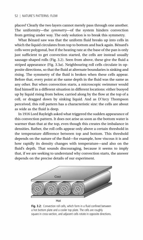
places? Clearly the two layers cannot merely pass through one another.
The uniformity—the symmetry—of the system hinders convection
from getting under way. The only solution is to break this symmetry.
What Benard saw was that the uniform fluid breaks up into cells in
which the liquid circulates from top to bottom and back again. Benard’s
cells were polygonal, but if the heating rate at the base of the pan is only
just sufficient to get convection started, the cells are instead usually
sausage-shaped rolls (Fig. 3.2). Seen from above, these give the fluid a
striped appearance (Fig. 3.3a). Neighbouring roll cells circulate in op-
posite directions, so that the fluid at alternate boundaries is sinking and
rising. The symmetry of the fluid is broken when these cells appear.
Before that, every point at the same depth in the fluid was the same as
any other. But when convection starts, a microscopic swimmer would
find himself in a different situation in different locations: either buoyed
up by liquid rising from below, carried along by the flow at the top of a
cell, or dragged down by sinking liquid. And as D’Arcy Thompson
perceived, this roll pattern has a characteristic size: the cells are about
as wide as the fluid is deep.
In 1916 Lord Rayleigh asked what triggered the sudden appearance of
this convection pattern. It does not arise as soon as the bottom water is
warmer than that at the top, even though this creates the imbalance in
densities. Rather, the roll cells appear only above a certain threshold in
the temperature difference between top and bottom. This threshold
depends on the nature of the fluid—for example, how viscous it is and
how rapidly its density changes with temperature—and also on the
fluid’s depth. That sounds discouraging, because it seems to imply
that, if we are seeking to understand why convection starts, the answer
depends on the precise details of our experiment.
Fig. 3.2: Convection roll cells, which form in a fluid confined betweena hot bottom plate and a cooler top plate. The cells are roughlysquare in cross-section, and adjacent cells rotate in opposite directions.
52 j NATURE’S PATTERNS: FLOW

But Rayleigh showed that the various factors that determine the
critical threshold for convection can be combined in a single quantity
that supplies a universal criterion for whether or not convection occurs.
Like the Reynolds number, this parameter, now called the Rayleigh
number, Ra, has no units: it is another dimensionless variable of fluid
dynamics. And like the Reynolds number, the Rayleigh number speci-
fies a ratio of forces—specifically, of the forces that promote convection
(the buoyancy of the fluid, which is determined in part by the tempera-
ture difference between the top and bottom) and those that oppose it
(the frictional forces that arise from the fluid’s viscosity, and the fluid’s
ability to conduct heat and thus to even out the temperature imbalance
without flowing at all). The reason convection does not arise as soon as
the bottom becomes warmer than the top is because the fluid motion
is opposed by friction. Only when the driving force (the temper-
ature difference) becomes big enough to overcome this resistance
do the convection cells appear. This corresponds to a Rayleigh number
of 1,708.
Just as we saw when using the Reynolds number to characterize fluid
flow, the beauty of treating the problem of convection by reference to
the Rayleigh number is that this number is then all we need worry
about (well, nearly all, as we shall see). Two different fluids in vessels of
different sizes and shapes will convect (or not) in the same way when
their Rayleigh number is the same. This means that one can map out
the generic behaviour of convecting fluids as a function of their Ray-
leigh number, without having to worry about whether the fluid is water,
oil, or glycerine. Rayleigh also showed that the roll cells that appear at
the onset of convection have a particular width that is very nearly (but
not exactly) equal to the depth of the fluid, so the rolls have an approxi-
mately square cross-section.
If the Rayleigh number is increased beyond its critical value of 1,708
to a value of several tens of thousands, the convection pattern can
switch abruptly to one in which there are essentially two sets of per-
pendicular rolls (Fig. 3.3b). At still higher values of Ra, the roll pattern
breaks down altogether and the cells take on a random polygonal
appearance called a spoke pattern (Fig. 3.3c). Unlike the rolls, this
pattern is not steady: the cells continually change shape over time. It
is, in fact, a turbulent form of convection.
The theory of fluid dynamics, which I shall outline in Chapter 6,
supplies equations for describing flow that are extremely hard to solve
ON A ROLL j 53
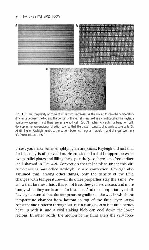
unless you make some simplifying assumptions. Rayleigh did just that
for his analysis of convection. He considered a fluid trapped between
two parallel plates and filling the gap entirely, so there is no free surface
(as I showed in Fig. 3.2). Convection that takes place under this cir-
cumstance is now called Rayleigh–Benard convection. Rayleigh also
assumed that (among other things) only the density of the fluid
changes with temperature—all its other properties stay the same. We
know that for most fluids this is not true: they get less viscous andmore
runny when they are heated, for instance. And most importantly of all,
Rayleigh assumed that the temperature gradient—the way in which the
temperature changes from bottom to top of the fluid layer—stays
constant and uniform throughout. But a rising blob of hot fluid carries
heat up with it, and a cool sinking blob can cool down the lower
regions. In other words, the motion of the fluid alters the very force
Fig. 3.3: The complexity of convection patterns increases as the driving force—the temperaturedifference between the top and the bottom of the vessel, measured as a quantity called the Rayleighnumber—increases. First there are simple roll cells (a). At higher Rayleigh numbers, roll cellsdevelop in the perpendicular direction too, so that the pattern consists of roughly square cells (b).At still higher Rayleigh numbers, the pattern becomes irregular (turbulent) and changes over time(c). (From Tritton, 1988.)
54 j NATURE’S PATTERNS: FLOW
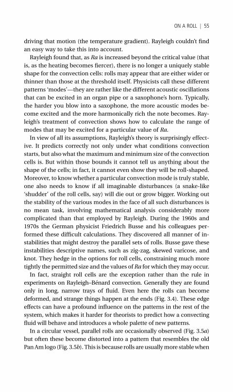
driving that motion (the temperature gradient). Rayleigh couldn’t find
an easy way to take this into account.
Rayleigh found that, as Ra is increased beyond the critical value (that
is, as the heating becomes fiercer), there is no longer a uniquely stable
shape for the convection cells: rolls may appear that are either wider or
thinner than those at the threshold itself. Physicists call these different
patterns ‘modes’—they are rather like the different acoustic oscillations
that can be excited in an organ pipe or a saxophone’s horn. Typically,
the harder you blow into a saxophone, the more acoustic modes be-
come excited and the more harmonically rich the note becomes. Ray-
leigh’s treatment of convection shows how to calculate the range of
modes that may be excited for a particular value of Ra.
In view of all its assumptions, Rayleigh’s theory is surprisingly effect-
ive. It predicts correctly not only under what conditions convection
starts, but alsowhat themaximum andminimum size of the convection
cells is. But within those bounds it cannot tell us anything about the
shape of the cells; in fact, it cannot even show they will be roll-shaped.
Moreover, to knowwhether a particular convectionmode is truly stable,
one also needs to know if all imaginable disturbances (a snake-like
‘shudder’ of the roll cells, say) will die out or grow bigger. Working out
the stability of the various modes in the face of all such disturbances is
no mean task, involving mathematical analysis considerably more
complicated than that employed by Rayleigh. During the 1960s and
1970s the German physicist Friedrich Busse and his colleagues per-
formed these difficult calculations. They discovered all manner of in-
stabilities that might destroy the parallel sets of rolls. Busse gave these
instabilities descriptive names, such as zig-zag, skewed varicose, and
knot. They hedge in the options for roll cells, constraining much more
tightly the permitted size and the values of Ra for which theymay occur.
In fact, straight roll cells are the exception rather than the rule in
experiments on Rayleigh–Benard convection. Generally they are found
only in long, narrow trays of fluid. Even here the rolls can become
deformed, and strange things happen at the ends (Fig. 3.4). These edge
effects can have a profound influence on the patterns in the rest of the
system, which makes it harder for theorists to predict how a convecting
fluid will behave and introduces a whole palette of new patterns.
In a circular vessel, parallel rolls are occasionally observed (Fig. 3.5a)
but often these become distorted into a pattern that resembles the old
PanAm logo (Fig. 3.5b). This is because rolls are usuallymore stablewhen
ON A ROLL j 55
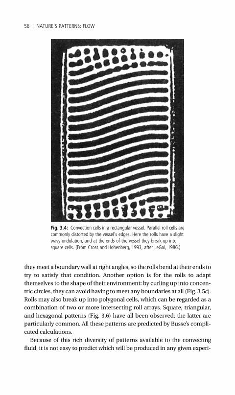
theymeet a boundarywall at right angles, so the rolls bend at their ends to
try to satisfy that condition. Another option is for the rolls to adapt
themselves to the shape of their environment: by curling up into concen-
tric circles, they can avoid having tomeet any boundaries at all (Fig. 3.5c).
Rolls may also break up into polygonal cells, which can be regarded as a
combination of two or more intersecting roll arrays. Square, triangular,
and hexagonal patterns (Fig. 3.6) have all been observed; the latter are
particularly common. All these patterns are predicted by Busse’s compli-
cated calculations.
Because of this rich diversity of patterns available to the convecting
fluid, it is not easy to predict which will be produced in any given experi-
Fig. 3.4: Convection cells in a rectangular vessel. Parallel roll cells arecommonly distorted by the vessel’s edges. Here the rolls have a slightwavy undulation, and at the ends of the vessel they break up intosquare cells. (From Cross and Hohenberg, 1993, after LeGal, 1986.)
56 j NATURE’S PATTERNS: FLOW

ment. When several alternative patterns are possible in principle for a
particular set of conditions, which is selected may depend on how the
system is prepared—that is, on the initial conditions and theway inwhich
these are changed to reach a specific set of experimental parameters.
Pattern formation is then dependent on the past history of the system.
Fig. 3.5: In a circular dish, roll cells take a variety of shapes. They may remain parallel (a), orcurve gently into a pattern resembling the old Pan-Am logo (b) to reduce the angle at whichthe rolls meet the wall. There are no such intersections at all if the cells take on the formof concentric circles (c). In (a) the fluid is carbon dioxide gas, in (b) it is argon gas, and in(c) water. (Images: a and c, David Cannell, University of California at Santa Barbara; b fromCross and Hohenberg, 1993, after Croquette, 1989.)
Fig. 3.6: Crossed roll cells may generate square or hexagonalpatterns, as seen here in convecting carbon dioxide gas. (Notice thatthere are still two circular rolls running around the perimeter.) (Image:David Cannell, University of California at Santa Barbara.)
ON A ROLL j 57
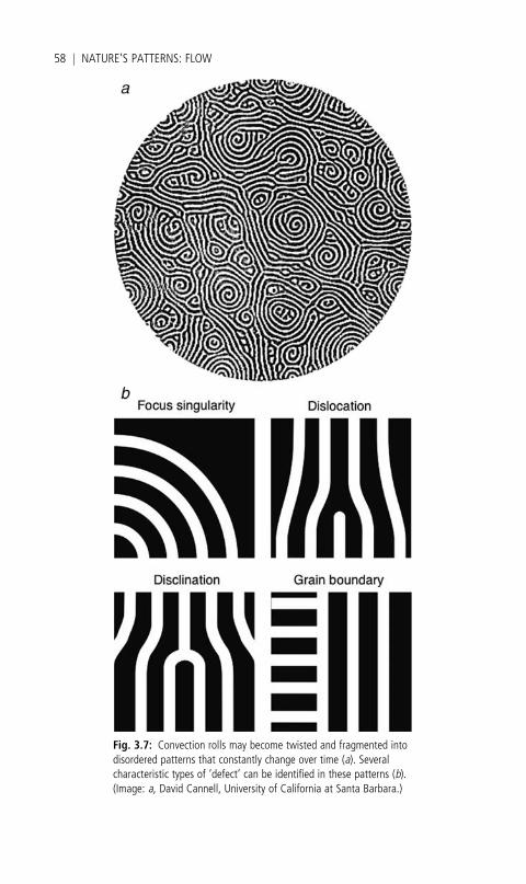
Fig. 3.7: Convection rolls may become twisted and fragmented intodisordered patterns that constantly change over time (a). Severalcharacteristic types of ‘defect’ can be identified in these patterns (b).(Image: a, David Cannell, University of California at Santa Barbara.)
58 j NATURE’S PATTERNS: FLOW
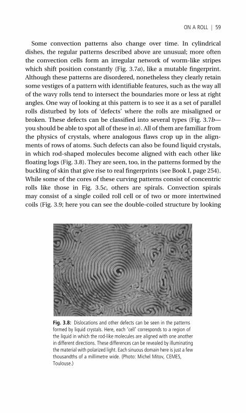
Some convection patterns also change over time. In cylindrical
dishes, the regular patterns described above are unusual; more often
the convection cells form an irregular network of worm-like stripes
which shift position constantly (Fig. 3.7a), like a mutable fingerprint.
Although these patterns are disordered, nonetheless they clearly retain
some vestiges of a pattern with identifiable features, such as the way all
of the wavy rolls tend to intersect the boundaries more or less at right
angles. One way of looking at this pattern is to see it as a set of parallel
rolls disturbed by lots of ‘defects’ where the rolls are misaligned or
broken. These defects can be classified into several types (Fig. 3.7b—
you should be able to spot all of these in a). All of them are familiar from
the physics of crystals, where analogous flaws crop up in the align-
ments of rows of atoms. Such defects can also be found liquid crystals,
in which rod-shaped molecules become aligned with each other like
floating logs (Fig. 3.8). They are seen, too, in the patterns formed by the
buckling of skin that give rise to real fingerprints (see Book I, page 254).
While some of the cores of these curving patterns consist of concentric
rolls like those in Fig. 3.5c, others are spirals. Convection spirals
may consist of a single coiled roll cell or of two or more intertwined
coils (Fig. 3.9; here you can see the double-coiled structure by looking
Fig. 3.8: Dislocations and other defects can be seen in the patternsformed by liquid crystals. Here, each ‘cell’ corresponds to a region ofthe liquid in which the rod-like molecules are aligned with one anotherin different directions. These differences can be revealed by illuminatingthe material with polarized light. Each sinuous domain here is just a fewthousandths of a millimetre wide. (Photo: Michel Mitov, CEMES,Toulouse.)
ON A ROLL j 59
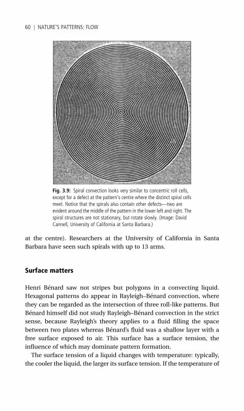
at the centre). Researchers at the University of California in Santa
Barbara have seen such spirals with up to 13 arms.
Surface matters
Henri Benard saw not stripes but polygons in a convecting liquid.
Hexagonal patterns do appear in Rayleigh–Benard convection, where
they can be regarded as the intersection of three roll-like patterns. But
Benard himself did not study Rayleigh–Benard convection in the strict
sense, because Rayleigh’s theory applies to a fluid filling the space
between two plates whereas Benard’s fluid was a shallow layer with a
free surface exposed to air. This surface has a surface tension, the
influence of which may dominate pattern formation.
The surface tension of a liquid changes with temperature: typically,
the cooler the liquid, the larger its surface tension. If the temperature of
Fig. 3.9: Spiral convection looks very similar to concentric roll cells,except for a defect at the pattern’s centre where the distinct spiral cellsmeet. Notice that the spirals also contain other defects—two areevident around the middle of the pattern in the lower left and right. Thespiral structures are not stationary, but rotate slowly. (Image: DavidCannell, University of California at Santa Barbara.)
60 j NATURE’S PATTERNS: FLOW
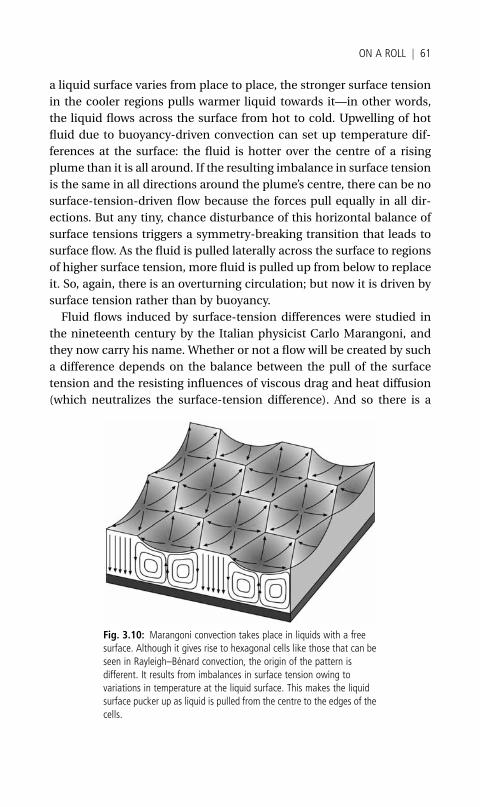
a liquid surface varies from place to place, the stronger surface tension
in the cooler regions pulls warmer liquid towards it—in other words,
the liquid flows across the surface from hot to cold. Upwelling of hot
fluid due to buoyancy-driven convection can set up temperature dif-
ferences at the surface: the fluid is hotter over the centre of a rising
plume than it is all around. If the resulting imbalance in surface tension
is the same in all directions around the plume’s centre, there can be no
surface-tension-driven flow because the forces pull equally in all dir-
ections. But any tiny, chance disturbance of this horizontal balance of
surface tensions triggers a symmetry-breaking transition that leads to
surface flow. As the fluid is pulled laterally across the surface to regions
of higher surface tension, more fluid is pulled up from below to replace
it. So, again, there is an overturning circulation; but now it is driven by
surface tension rather than by buoyancy.
Fluid flows induced by surface-tension differences were studied in
the nineteenth century by the Italian physicist Carlo Marangoni, and
they now carry his name. Whether or not a flow will be created by such
a difference depends on the balance between the pull of the surface
tension and the resisting influences of viscous drag and heat diffusion
(which neutralizes the surface-tension difference). And so there is a
Fig. 3.10: Marangoni convection takes place in liquids with a freesurface. Although it gives rise to hexagonal cells like those that can beseen in Rayleigh–Benard convection, the origin of the pattern isdifferent. It results from imbalances in surface tension owing tovariations in temperature at the liquid surface. This makes the liquidsurface pucker up as liquid is pulled from the centre to the edges of thecells.
ON A ROLL j 61
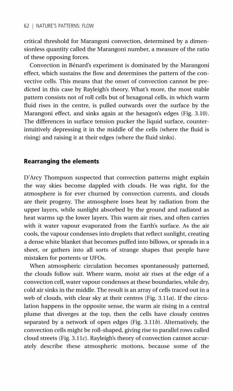
critical threshold for Marangoni convection, determined by a dimen-
sionless quantity called the Marangoni number, a measure of the ratio
of these opposing forces.
Convection in Benard’s experiment is dominated by the Marangoni
effect, which sustains the flow and determines the pattern of the con-
vective cells. This means that the onset of convection cannot be pre-
dicted in this case by Rayleigh’s theory. What’s more, the most stable
pattern consists not of roll cells but of hexagonal cells, in which warm
fluid rises in the centre, is pulled outwards over the surface by the
Marangoni effect, and sinks again at the hexagon’s edges (Fig. 3.10).
The differences in surface tension pucker the liquid surface, counter-
intuitively depressing it in the middle of the cells (where the fluid is
rising) and raising it at their edges (where the fluid sinks).
Rearranging the elements
D’Arcy Thompson suspected that convection patterns might explain
the way skies become dappled with clouds. He was right, for the
atmosphere is for ever churned by convection currents, and clouds
are their progeny. The atmosphere loses heat by radiation from the
upper layers, while sunlight absorbed by the ground and radiated as
heat warms up the lower layers. This warm air rises, and often carries
with it water vapour evaporated from the Earth’s surface. As the air
cools, the vapour condenses into droplets that reflect sunlight, creating
a dense white blanket that becomes puffed into billows, or spreads in a
sheet, or gathers into all sorts of strange shapes that people have
mistaken for portents or UFOs.
When atmospheric circulation becomes spontaneously patterned,
the clouds follow suit. Where warm, moist air rises at the edge of a
convection cell, water vapour condenses at these boundaries, while dry,
cold air sinks in the middle. The result is an array of cells traced out in a
web of clouds, with clear sky at their centres (Fig. 3.11a). If the circu-
lation happens in the opposite sense, the warm air rising in a central
plume that diverges at the top, then the cells have cloudy centres
separated by a network of open edges (Fig. 3.11b). Alternatively, the
convection cells might be roll-shaped, giving rise to parallel rows called
cloud streets (Fig. 3.11c). Rayleigh’s theory of convection cannot accur-
ately describe these atmospheric motions, because some of the
62 j NATURE’S PATTERNS: FLOW
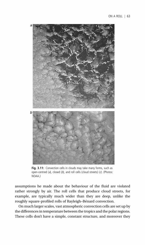
assumptions he made about the behaviour of the fluid are violated
rather strongly by air. The roll cells that produce cloud streets, for
example, are typically much wider than they are deep, unlike the
roughly square-profiled rolls of Rayleigh–Benard convection.
Onmuch larger scales, vast atmospheric convection cells are set up by
thedifferences in temperature between the tropics and thepolar regions.
These cells don’t have a simple, constant structure, and moreover they
Fig. 3.11: Convection cells in clouds may take many forms, such asopen-centred (a), closed (b), and roll cells (cloud streets) (c). (Photos:NOAA.)
ON A ROLL j 63
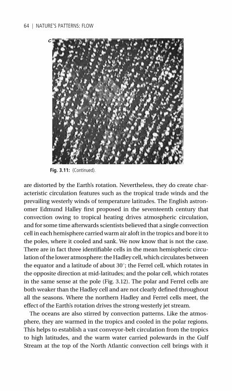
are distorted by the Earth’s rotation. Nevertheless, they do create char-
acteristic circulation features such as the tropical trade winds and the
prevailing westerly winds of temperature latitudes. The English astron-
omer Edmund Halley first proposed in the seventeenth century that
convection owing to tropical heating drives atmospheric circulation,
and for some time afterwards scientists believed that a single convection
cell in eachhemisphere carriedwarmair aloft in the tropics and bore it to
the poles, where it cooled and sank. We now know that is not the case.
There are in fact three identifiable cells in the mean hemispheric circu-
lationof the lower atmosphere: theHadley cell, which circulates between
the equator and a latitude of about 308; the Ferrel cell, which rotates in
the opposite direction at mid-latitudes; and the polar cell, which rotates
in the same sense at the pole (Fig. 3.12). The polar and Ferrel cells are
both weaker than the Hadley cell and are not clearly defined throughout
all the seasons. Where the northern Hadley and Ferrel cells meet, the
effect of the Earth’s rotation drives the strong westerly jet stream.
The oceans are also stirred by convection patterns. Like the atmos-
phere, they are warmed in the tropics and cooled in the polar regions.
This helps to establish a vast conveyor-belt circulation from the tropics
to high latitudes, and the warm water carried polewards in the Gulf
Stream at the top of the North Atlantic convection cell brings with it
Fig. 3.11: (Continued).
64 j NATURE’S PATTERNS: FLOW

heat that keeps northern Europe temperate (Fig. 3.13). This circulation
pattern is not purely thermal (heat-driven), however. The density of sea
water is also determined by the amount of dissolved salt it contains: the
more saline the water, the denser it is. The salinity depends on evapor-
ation, which removes water vapour and leaves behind saltier water, and
also on freezing, since ice doesn’t accommodate much salt. Thus the
large-scale pattern of ocean convection is influenced by evaporation in
the tropics and freezing at the poles: together, these processes give rise
Fig. 3.12: Large-scale convection in the Earth’s atmosphere isorganized into three roll-like cells in each hemisphere: the Hadleycell between the equator and about 308 latitude, the Ferrel cell atmid-latitudes, and the polar cells.
Fig. 3.13: Convection in the oceans, driven by differences in water temperature and saltiness,creates a global pattern of conveyor-belt circulation that carries warm, less salty water along theupper belt and cold, more salty water along the lower one.
ON A ROLL j 65
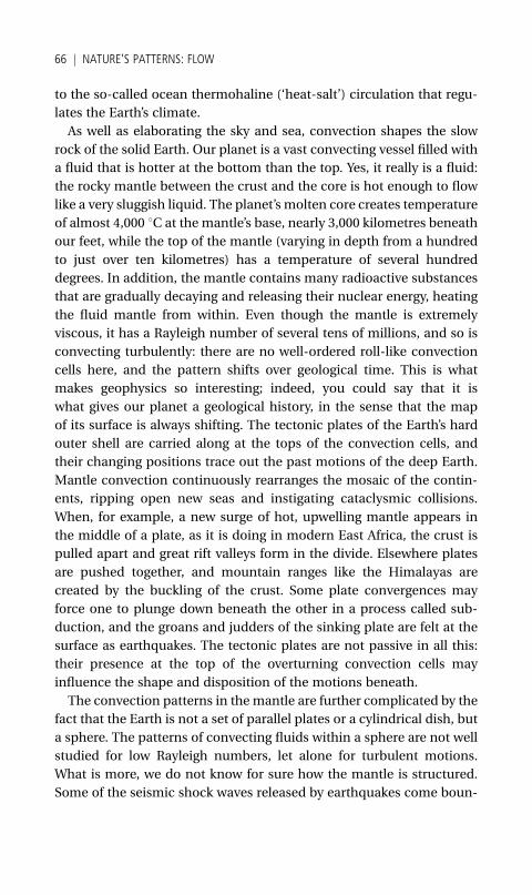
to the so-called ocean thermohaline (‘heat-salt’) circulation that regu-
lates the Earth’s climate.
As well as elaborating the sky and sea, convection shapes the slow
rock of the solid Earth. Our planet is a vast convecting vessel filled with
a fluid that is hotter at the bottom than the top. Yes, it really is a fluid:
the rocky mantle between the crust and the core is hot enough to flow
like a very sluggish liquid. The planet’s molten core creates temperature
of almost 4,000 8C at the mantle’s base, nearly 3,000 kilometres beneath
our feet, while the top of the mantle (varying in depth from a hundred
to just over ten kilometres) has a temperature of several hundred
degrees. In addition, the mantle contains many radioactive substances
that are gradually decaying and releasing their nuclear energy, heating
the fluid mantle from within. Even though the mantle is extremely
viscous, it has a Rayleigh number of several tens of millions, and so is
convecting turbulently: there are no well-ordered roll-like convection
cells here, and the pattern shifts over geological time. This is what
makes geophysics so interesting; indeed, you could say that it is
what gives our planet a geological history, in the sense that the map
of its surface is always shifting. The tectonic plates of the Earth’s hard
outer shell are carried along at the tops of the convection cells, and
their changing positions trace out the past motions of the deep Earth.
Mantle convection continuously rearranges the mosaic of the contin-
ents, ripping open new seas and instigating cataclysmic collisions.
When, for example, a new surge of hot, upwelling mantle appears in
the middle of a plate, as it is doing in modern East Africa, the crust is
pulled apart and great rift valleys form in the divide. Elsewhere plates
are pushed together, and mountain ranges like the Himalayas are
created by the buckling of the crust. Some plate convergences may
force one to plunge down beneath the other in a process called sub-
duction, and the groans and judders of the sinking plate are felt at the
surface as earthquakes. The tectonic plates are not passive in all this:
their presence at the top of the overturning convection cells may
influence the shape and disposition of the motions beneath.
The convection patterns in the mantle are further complicated by the
fact that the Earth is not a set of parallel plates or a cylindrical dish, but
a sphere. The patterns of convecting fluids within a sphere are not well
studied for low Rayleigh numbers, let alone for turbulent motions.
What is more, we do not know for sure how the mantle is structured.
Some of the seismic shock waves released by earthquakes come boun-
66 j NATURE’S PATTERNS: FLOW
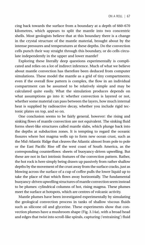
cing back towards the surface from a boundary at a depth of 660–670
kilometres, which appears to split the mantle into two concentric
shells. Most geologists believe that at this boundary there is a change
in the crystal structure of the mantle material, brought about by the
intense pressures and temperatures at these depths. Do the convection
cells punch their way straight through this boundary, or do cells circu-
late independently in the upper and lower mantle?
Exploring these literally deep questions experimentally is compli-
cated and relies on a lot of indirect inference. Much of what we believe
about mantle convection has therefore been deduced from computer
simulations. These model the mantle as a grid of tiny compartments;
even if the overall flow pattern is complex, the flow in an individual
compartment can be assumed to be relatively simple and may be
calculated quite easily. What the simulation produces depends on
what assumptions go into it: whether convection is layered or not,
whether somematerial can pass between the layers, howmuch internal
heat is supplied by radioactive decay, whether you include rigid tec-
tonic plates on top, and so on.
One conclusion seems to be fairly general, however: the rising and
sinking flows of mantle convection are not equivalent. The sinking fluid
forms sheet-like structures called mantle slabs, which plunge back into
the depths at subduction zones. It is tempting to regard the oceanic
fissures where hot magma wells up to form new ocean crust, such as
the Mid-Atlantic Ridge that cleaves the Atlantic almost from pole to pole
or the East Pacific Rise off the west coast of South America, as the
corresponding counterflows: sheets of buoyancy-driven upwelling. But
these are not in fact intrinsic features of the convection pattern. Rather,
the hot rock is here simply being drawn up passively from rather shallow
depths by themovement of the crust away from the surface cracks, just as
blowing across the surface of a cup of coffee pulls the lower liquid up to
take the place of that which flows away horizontally. The fundamental
buoyancy-drivenupwelling structuresofmantle convection seeminstead
to be plumes: cylindrical columns of hot, rising magma. These plumes
meet the surface at hotspots, which are centres of volcanic activity.
Mantle plumes have been investigated experimentally by simulating
the geological convection process in tanks of shallow viscous fluids
such as silicone oil and glycerine. These experiments show that con-
vection plumes have a mushroom shape (Fig. 3.14a), with a broad head
and edges that twist into scroll-like spirals, capturing (‘entraining’) fluid
ON A ROLL j 67
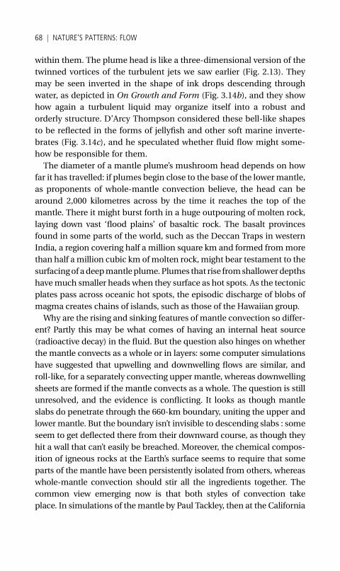
within them. The plume head is like a three-dimensional version of the
twinned vortices of the turbulent jets we saw earlier (Fig. 2.13). They
may be seen inverted in the shape of ink drops descending through
water, as depicted in On Growth and Form (Fig. 3.14b), and they show
how again a turbulent liquid may organize itself into a robust and
orderly structure. D’Arcy Thompson considered these bell-like shapes
to be reflected in the forms of jellyfish and other soft marine inverte-
brates (Fig. 3.14c), and he speculated whether fluid flow might some-
how be responsible for them.
The diameter of a mantle plume’s mushroom head depends on how
far it has travelled: if plumes begin close to the base of the lowermantle,
as proponents of whole-mantle convection believe, the head can be
around 2,000 kilometres across by the time it reaches the top of the
mantle. There it might burst forth in a huge outpouring of molten rock,
laying down vast ‘flood plains’ of basaltic rock. The basalt provinces
found in some parts of the world, such as the Deccan Traps in western
India, a region covering half a million square km and formed frommore
than half a million cubic km ofmolten rock, might bear testament to the
surfacingof adeepmantleplume. Plumes that rise fromshallowerdepths
havemuch smaller heads when they surface as hot spots. As the tectonic
plates pass across oceanic hot spots, the episodic discharge of blobs of
magma creates chains of islands, such as those of the Hawaiian group.
Why are the rising and sinking features of mantle convection so differ-
ent? Partly this may be what comes of having an internal heat source
(radioactive decay) in the fluid. But the question also hinges on whether
the mantle convects as a whole or in layers: some computer simulations
have suggested that upwelling and downwelling flows are similar, and
roll-like, for a separately convecting upper mantle, whereas downwelling
sheets are formed if the mantle convects as a whole. The question is still
unresolved, and the evidence is conflicting. It looks as though mantle
slabs do penetrate through the 660-km boundary, uniting the upper and
lower mantle. But the boundary isn’t invisible to descending slabs : some
seem to get deflected there from their downward course, as though they
hit a wall that can’t easily be breached. Moreover, the chemical compos-
ition of igneous rocks at the Earth’s surface seems to require that some
parts of the mantle have been persistently isolated from others, whereas
whole-mantle convection should stir all the ingredients together. The
common view emerging now is that both styles of convection take
place. In simulations of themantle by Paul Tackley, then at the California
68 j NATURE’S PATTERNS: FLOW

Institute of Technology, and his colleagues, the flow pattern was organ-
ized into hot rising plumes and cold sinking sheets. The plumeswere able
to force a passage from thebaseof themantle right to the top. But the cold
sinking sheets (themantle slabs) generally stopped at the 660-kmbound-
ary, where the cold, dense fluid accumulated in spreading puddles.When
Fig. 3.14: Convectionin viscous fluids at highRayleigh number createsmushroom-shaped risingplumes (a). Such featuresare thought to exist in theEarth’s mantle. Where aplume breaks throughthe crust, there isvolcanic activity. D’ArcyThompson recognizedthis same form invertedin the descent of inkdroplets in water (b), andhe also found it echoed inthe shapes of somejellyfish, such asSyncoryme (c). (Photo: a,Ross Griffiths, AustralianNational University,Canberra.)
ON A ROLL j 69
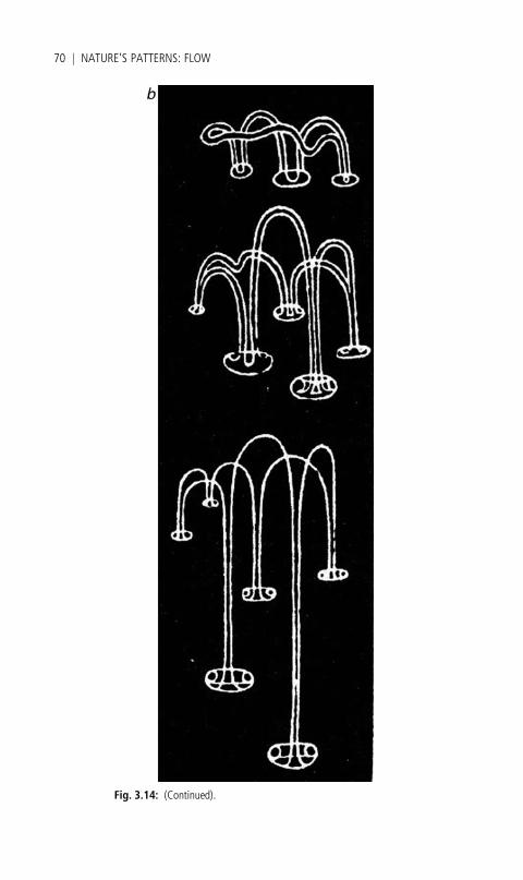
Fig. 3.14: (Continued).
70 j NATURE’S PATTERNS: FLOW
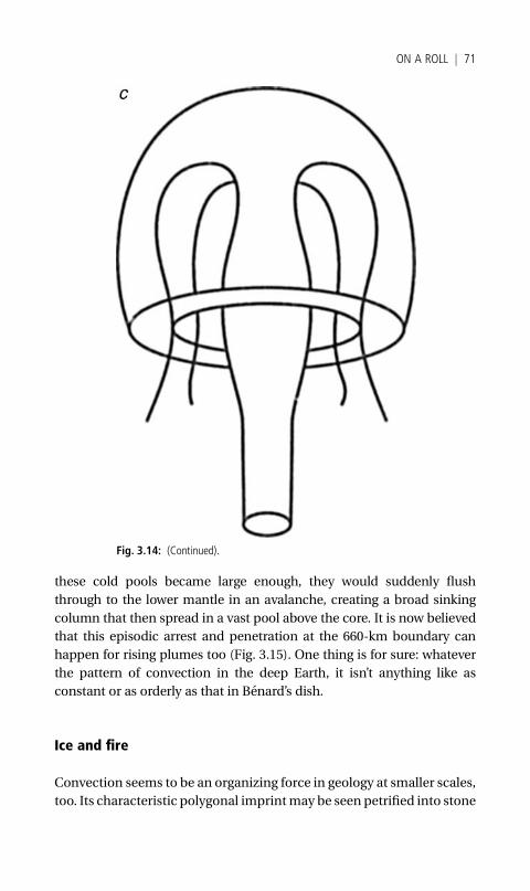
these cold pools became large enough, they would suddenly flush
through to the lower mantle in an avalanche, creating a broad sinking
column that then spread in a vast pool above the core. It is now believed
that this episodic arrest and penetration at the 660-km boundary can
happen for rising plumes too (Fig. 3.15). One thing is for sure: whatever
the pattern of convection in the deep Earth, it isn’t anything like as
constant or as orderly as that in Benard’s dish.
Ice and fire
Convection seems to be an organizing force in geology at smaller scales,
too. Its characteristic polygonal imprintmay be seen petrified into stone
Fig. 3.14: (Continued).
ON A ROLL j 71
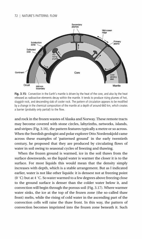
and rock in the frozenwastes of Alaska andNorway. These remote tracts
may become covered with stone circles, labyrinths, networks, islands,
and stripes (Fig. 3.16), the pattern features typically ametre or so across.
When the Swedish geologist and polar explorer OttoNordenskjold came
across these examples of ‘patterned ground’ in the early twentieth
century, he proposed that they are produced by circulating flows of
water in soil owing to seasonal cycles of freezing and thawing.
When the frozen ground is warmed, ice in the soil thaws from the
surface downwards, so the liquid water is warmer the closer it is to the
surface. For most liquids this would mean that the density simply
increases with depth, which is a stable arrangement. But as I indicated
earlier, water is not like other liquids: it is densest not at freezing point
(0 8C) but at 4 8C. Sowater warmed to a fewdegrees above freezing close
to the ground surface is denser than the colder water below it, and
convection will begin through the porous soil (Fig. 3.17). Where warmer
water sinks, the ice at the top of the frozen zone (the so-called thaw
front) melts, while the rising of cold water in the ascending part of the
convection cells will raise the thaw front. In this way, the pattern of
convection becomes imprinted into the frozen zone beneath it. Such
Fig. 3.15: Convection in the Earth’s mantle is driven by the heat of the core, and also by the heatreleased as radioactive elements decay within the mantle. It tends to produce rising plumes of hot,sluggish rock, and descending slab of cooler rock. The pattern of circulation appears to be modifiedby a change in the chemical composition of the mantle at a depth of around 660 km, which createsa barrier (probably only partial) to the flow.
72 j NATURE’S PATTERNS: FLOW
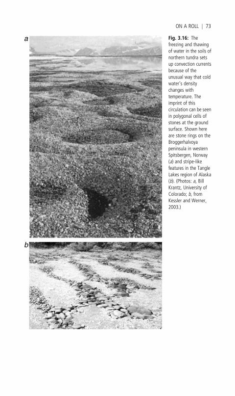
Fig. 3.16: Thefreezing and thawingof water in the soils ofnorthern tundra setsup convection currentsbecause of theunusual way that coldwater’s densitychanges withtemperature. Theimprint of thiscirculation can be seenin polygonal cells ofstones at the groundsurface. Shown hereare stone rings on theBroggerhalvoyapeninsula in westernSpitsbergen, Norway(a) and stripe-likefeatures in the TangleLakes region of Alaska(b). (Photos: a, BillKrantz, University ofColorado; b, fromKessler and Werner,2003.)
ON A ROLL j 73

polygonal patterns can also be foundon the beds of northern lakeswhen
the water is shallow enough to freeze down into the lake bed (Fig. 3.18).
William Krantz and colleagues at the University of Colorado at Boul-
der have shown how this process might account for the orderly piles of
stones on the surface. They say that sub-surface stones are gathered in
the troughs of the corrugated thaw front, and then brought to the
surface by ‘frost heaving’, a process familiar to farmers, that happens
when soil freezes. So a field that freezes during a frost and then thaws
Fig. 3.17: As water circulates in convection cells through the soil, the pattern istransferred to the ‘thaw front’, below which the ground remains frozen. Stonesgather in the troughs of the thaw front, and are brought to the surface by ‘frostheaving’ in the soil.
Fig. 3.18: Freeze-thaw cycles of groundwater at the edge of this Norwegian lake have producedconvection cells traced out by stones on the lake bed. (Photo: Bill Krantz, University of Colorado.)
74 j NATURE’S PATTERNS: FLOW
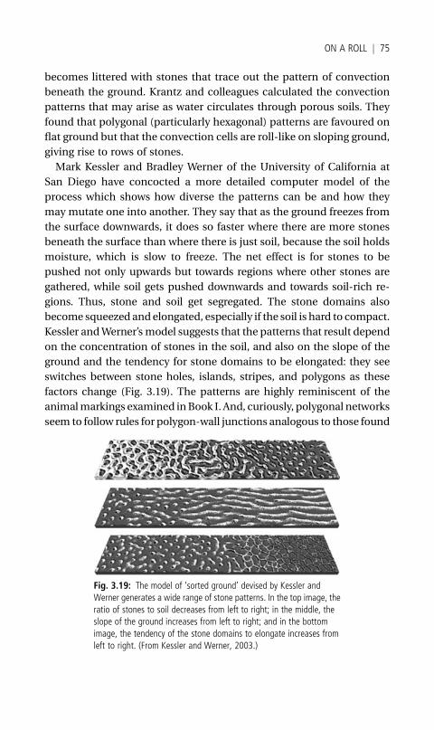
becomes littered with stones that trace out the pattern of convection
beneath the ground. Krantz and colleagues calculated the convection
patterns that may arise as water circulates through porous soils. They
found that polygonal (particularly hexagonal) patterns are favoured on
flat ground but that the convection cells are roll-like on sloping ground,
giving rise to rows of stones.
Mark Kessler and Bradley Werner of the University of California at
San Diego have concocted a more detailed computer model of the
process which shows how diverse the patterns can be and how they
may mutate one into another. They say that as the ground freezes from
the surface downwards, it does so faster where there are more stones
beneath the surface than where there is just soil, because the soil holds
moisture, which is slow to freeze. The net effect is for stones to be
pushed not only upwards but towards regions where other stones are
gathered, while soil gets pushed downwards and towards soil-rich re-
gions. Thus, stone and soil get segregated. The stone domains also
become squeezed andelongated, especially if the soil is hard to compact.
Kessler andWerner’s model suggests that the patterns that result depend
on the concentration of stones in the soil, and also on the slope of the
ground and the tendency for stone domains to be elongated: they see
switches between stone holes, islands, stripes, and polygons as these
factors change (Fig. 3.19). The patterns are highly reminiscent of the
animalmarkings examined inBook I. And, curiously, polygonal networks
seem to follow rules for polygon-wall junctions analogous to those found
Fig. 3.19: The model of ‘sorted ground’ devised by Kessler andWerner generates a wide range of stone patterns. In the top image, theratio of stones to soil decreases from left to right; in the middle, theslope of the ground increases from left to right; and in the bottomimage, the tendency of the stone domains to elongate increases fromleft to right. (From Kessler and Werner, 2003.)
ON A ROLL j 75
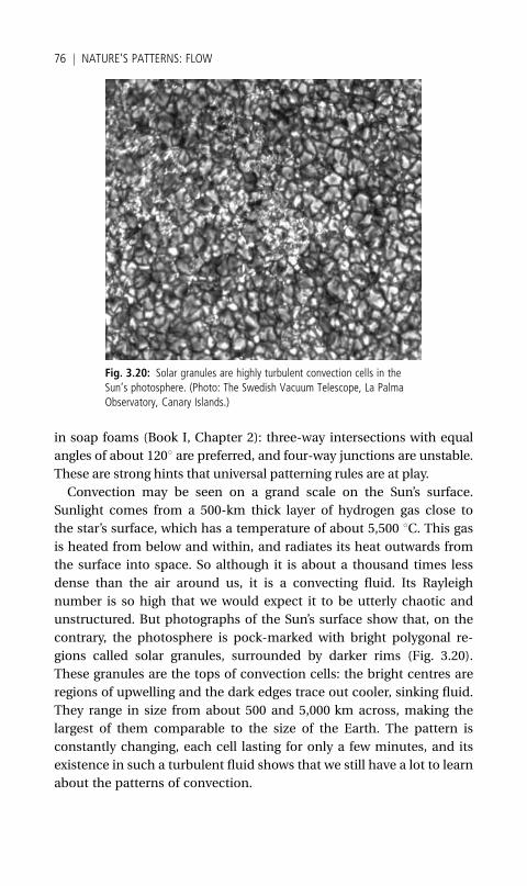
in soap foams (Book I, Chapter 2): three-way intersections with equal
angles of about 1208 are preferred, and four-way junctions are unstable.
These are strong hints that universal patterning rules are at play.
Convection may be seen on a grand scale on the Sun’s surface.
Sunlight comes from a 500-km thick layer of hydrogen gas close to
the star’s surface, which has a temperature of about 5,500 8C. This gasis heated from below and within, and radiates its heat outwards from
the surface into space. So although it is about a thousand times less
dense than the air around us, it is a convecting fluid. Its Rayleigh
number is so high that we would expect it to be utterly chaotic and
unstructured. But photographs of the Sun’s surface show that, on the
contrary, the photosphere is pock-marked with bright polygonal re-
gions called solar granules, surrounded by darker rims (Fig. 3.20).
These granules are the tops of convection cells: the bright centres are
regions of upwelling and the dark edges trace out cooler, sinking fluid.
They range in size from about 500 and 5,000 km across, making the
largest of them comparable to the size of the Earth. The pattern is
constantly changing, each cell lasting for only a few minutes, and its
existence in such a turbulent fluid shows that we still have a lot to learn
about the patterns of convection.
Fig. 3.20: Solar granules are highly turbulent convection cells in theSun’s photosphere. (Photo: The Swedish Vacuum Telescope, La PalmaObservatory, Canary Islands.)
76 j NATURE’S PATTERNS: FLOW
4Riddle of the DunesWhen Grains Get Together
IT would be easy to suppose that Ralph Alger Bagnold, rather like
T. E. Lawrence, went initially to the desert because of the army, and
ended up staying in the army because of the desert. He was by all
accounts a good soldier, but one cannot help thinking his mind must
have been only half on the job, for he could not suppress his scientific
instinct for enquiry even in the most unlikely circumstances. Trained as
an engineer, he joined the British Army’s Royal Engineers in 1915 and
found himself posted to Egypt and India, where he fell in love with the
deserts. By the 1920s he was spending his leave exploring these ‘seas of
sand’, joining the 1929 expedition in search of the legendary city of
Zerzura west of the Nile that was led by Laszlo Almasy, the Hungarian
nobleman who inspired Michael Ondaatje’s novel The English Patient.
‘We forgave Bagnold everything’, says Ondaatje’s Almasy, ‘for the way
he wrote about dunes.’ That is indeed what Bagnold did, and with such
perception and insight that his 1941 bookThe Physics of Blown Sand and
Desert Dunes became the standard work on dune formation for many
decades. Inspired by his observations in Libya and informed by wind-
tunnel experiments in England, Bagnold set out to explain how sand
grains are organized by the desert wind into structures ranging from
ripples the size of your fingers to undulations several kilometres across.
I cannot better Bagnold’s description of the basic dilemma posed by
the patterns of sand dunes. ‘Instead of finding chaos and disorder,’ he
wrote,
the observer never fails to be amazed at a simplicity of form, an exactitude of
repetition and a geometric order unknown in nature on a scale larger than that
of crystalline structure. In places vast accumulations of sand weighing millions
of tons move inexorably in regular formation, over the surface of the country,
growing, retaining their shape, even breeding, in a manner which, by its gro-
tesque imitation of life, is vaguely disturbing to an imaginative mind.
What Bagnold is really saying here, though lacking the modern term, is
that dunes are self-organized. Wind alone has no intrinsic capacity to
make these stripes and crescents and other fantastic shapes, nor to set
their scale. Sand ripples and dunes are a conspiracy of grains, a pattern
that emerges from the interplay of windborne movement, collision-
driven piling up, and slope-shaving avalanches. The formation of sand
dunes is not only one of themost fertile of pattern-creating processes; it
is also something of an archetype, an exemplary demonstration of how
such patterns lie in wait in systems of many interacting parts, even
though no amount of close inspection of the components will reveal
them. We will see it is no coincidence that some of these patterns again
display characteristic, seemingly universal features that we have seen
before.
There is something deeply odd about grains and powders. They are
made of solid stuff—sand is mostly quartz, hard and crystalline—and
yet they flow. Sand supports our weight, but we can pour it from a cup.
An extreme and rather terrible example of this Janus aspect can be seen
during some earthquakes, such as that which shook the Marina district
of San Francisco Bay in October 1989. Many of the houses there were
sent tumbling as a segment of the San Andreas Fault slipped, and
although miraculously there was no loss of life, hundreds of millions
of dollars’ worth of damage was done. Yet elsewhere in the bay area
there was nothing like this degree of destruction. What brought low the
Marina district is that it was built on sand-rich landfill sites. When the
earth shook, these wet, sandy soils turned to a slurry that flowed like
treacle. This property of a granular substance, naturally enough called
liquefaction, is well known to seismologists and civil engineers. It is one
of the most dramatic manifestations of the fact that a granular sub-
stance is a peculiar state of matter.
Engineers and geologists urgently need to understand such behav-
iour, and not only to gauge earthquake hazards. All manner of indus-
trial substances are routinely handled in the form of granular powders,
from cement to drugs to breakfast cereals, nails, nuts, and bolts. Graini-
ness is everywhere in the geological world: it dictates the behaviour of
landslides, the transport of sediments, and the shape and evolution of
deserts, beaches, soils, and stony ground. There are old rules of thumb
for predicting how grains behave, but only in recent years have scien-
tists begun to appreciate that to attain more fundamental understand-
ing they must invent new physics.
Strange things happen in grains. Shaking together different kinds of
grain canmix them up, or, on the contrary, may have the opposite effect
78 j NATURE’S PATTERNS: FLOW
of segregating them. Sound waves can bend around corners as they
travel through sand. The stress beneath a sand pile is smallest where
the pile is highest. Yet the pressure at the bottom of a tall column of
sand is the same regardless of the column’s height, which is why a sand
glass is a good timekeeper: the sand leaks out at a steady rate even
though the column gets smaller.
Shifting sands
Not all deserts are sandy, and not all sands are piled into dunes; but it is
the dune (Plate 6), which is found within only 20 per cent of the world’s
deserts, that defines our archetypal desert imagery. These seas of sand
are almost barren yet intensely beautiful, both terrifying and holy.
North Africans say that the desert is the Garden of Allah, scoured of
life so that he may walk there in peace.
Desert dunes range in width from a few metres to several kilometres,
andmay themselves be organized into complexmega–dunes, sometimes
called draas after their name in North Africa, which can be up to several
kilometres broad. Moreover, dunes come in a variety of shapes; indeed,
there are so many varieties, with region-specific names derived from the
local language, that even geomorphologists have trouble keeping track of
them. At the smallest scale, the desert floor is wrinkled into little wavy
ridges typically about the width of your arm (Fig. 4.1). The crests of these
ripples may be spaced as little as half a centimetre apart, or as much as
several metres. Bagnold sought to explain why wind-blown sand gets
deposited in this wrinkled pattern. In today’s terminology, we would say
that what he proposed is an example of a growth instability driven by
positive feedback, so that small disturbances get bigger.
Let’s start with a flat sandy plain, across which a steady wind is
blowing. The wind continually picks up grains and dumps them else-
where. If the wind blows always in the same direction, the plain is
gradually moved en masse upwind; the borders of deserts get shifted
around this way. But wouldn’t we expect the grains simply to be redis-
tributed at random, so that the sand surface stays smooth?
That is what you might think; but Bagnold’s growth instability makes
the flatness prone to wrinkling. Imagine that, purely by chance, a little
bump appears where slightly more sand has been dumped than else-
where—that is to be expected if the scattering of grains is truly random.
The windward side of the bump (called the stoss side) is now higher
RIDDLE OF THE DUNES j 79
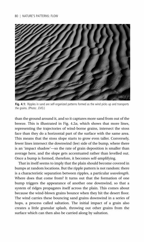
than the ground around it, and so it captures more sand from out of the
breeze. This is illustrated in Fig. 4.2a, which shows that more lines,
representing the trajectories of wind-borne grains, intersect the stoss
face than they do a horizontal part of the surface with the same area.
This means that the stoss slope starts to grow even taller. Conversely,
fewer lines intersect the downwind (lee) side of the bump, where there
is an ‘impact shadow’—so the rate of grain deposition is smaller than
average here, and the slope gets accentuated rather than levelled out.
Once a bump is formed, therefore, it becomes self-amplifying.
That in itself seems to imply that the plain should become covered in
bumps at random locations. But the ripple pattern is not random: there
is a characteristic separation between ripples, a particular wavelength.
Where does that come from? It turns out that the formation of one
bump triggers the appearance of another one downwind, so that a
system of ridges propagates itself across the plain. This comes about
because the wind-blown grains bounce when they hit the desert floor.
The wind carries these bouncing sand grains downwind in a series of
hops, a process called saltation. The initial impact of a grain also
creates a little granular splash, throwing out other grains from the
surface which can then also be carried along by saltation.
Fig. 4.1: Ripples in sand are self-organized patterns formed as the wind picks up and transportsthe grains. (Photo: .EVO.)
80 j NATURE’S PATTERNS: FLOW
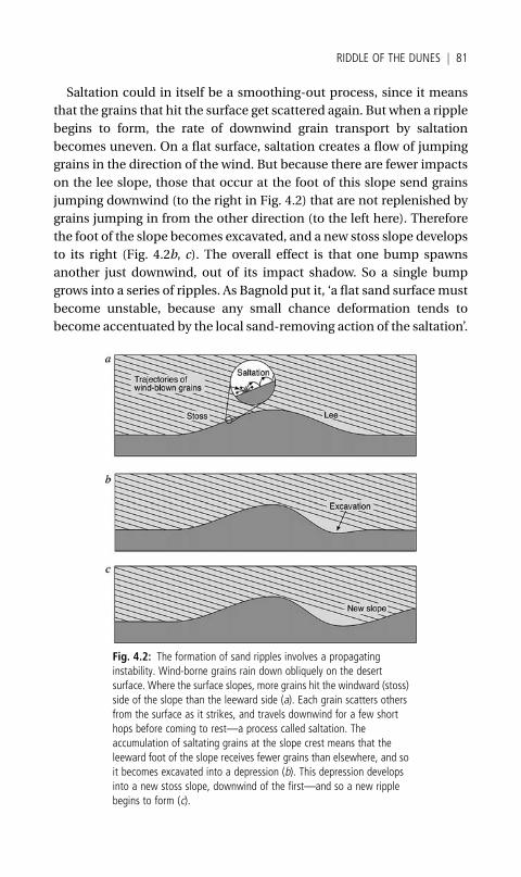
Saltation could in itself be a smoothing-out process, since it means
that the grains that hit the surface get scattered again. But when a ripple
begins to form, the rate of downwind grain transport by saltation
becomes uneven. On a flat surface, saltation creates a flow of jumping
grains in the direction of the wind. But because there are fewer impacts
on the lee slope, those that occur at the foot of this slope send grains
jumping downwind (to the right in Fig. 4.2) that are not replenished by
grains jumping in from the other direction (to the left here). Therefore
the foot of the slope becomes excavated, and a new stoss slope develops
to its right (Fig. 4.2b, c). The overall effect is that one bump spawns
another just downwind, out of its impact shadow. So a single bump
grows into a series of ripples. As Bagnold put it, ‘a flat sand surfacemust
become unstable, because any small chance deformation tends to
become accentuated by the local sand-removing action of the saltation’.
Fig. 4.2: The formation of sand ripples involves a propagatinginstability. Wind-borne grains rain down obliquely on the desertsurface. Where the surface slopes, more grains hit the windward (stoss)side of the slope than the leeward side (a). Each grain scatters othersfrom the surface as it strikes, and travels downwind for a few shorthops before coming to rest—a process called saltation. Theaccumulation of saltating grains at the slope crest means that theleeward foot of the slope receives fewer grains than elsewhere, and soit becomes excavated into a depression (b). This depression developsinto a new stoss slope, downwind of the first—and so a new ripplebegins to form (c).
RIDDLE OF THE DUNES j 81
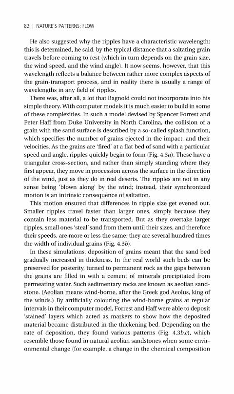
He also suggested why the ripples have a characteristic wavelength:
this is determined, he said, by the typical distance that a saltating grain
travels before coming to rest (which in turn depends on the grain size,
the wind speed, and the wind angle). It now seems, however, that this
wavelength reflects a balance between rather more complex aspects of
the grain-transport process, and in reality there is usually a range of
wavelengths in any field of ripples.
There was, after all, a lot that Bagnold could not incorporate into his
simple theory. With computer models it is much easier to build in some
of these complexities. In such a model devised by Spencer Forrest and
Peter Haff from Duke University in North Carolina, the collision of a
grain with the sand surface is described by a so-called splash function,
which specifies the number of grains ejected in the impact, and their
velocities. As the grains are ‘fired’ at a flat bed of sand with a particular
speed and angle, ripples quickly begin to form (Fig. 4.3a). These have a
triangular cross-section, and rather than simply standing where they
first appear, they move in procession across the surface in the direction
of the wind, just as they do in real deserts. The ripples are not in any
sense being ‘blown along’ by the wind; instead, their synchronized
motion is an intrinsic consequence of saltation.
This motion ensured that differences in ripple size get evened out.
Smaller ripples travel faster than larger ones, simply because they
contain less material to be transported. But as they overtake larger
ripples, small ones ‘steal’sand from them until their sizes, and therefore
their speeds, are more or less the same: they are several hundred times
the width of individual grains (Fig. 4.3b).
In these simulations, deposition of grains meant that the sand bed
gradually increased in thickness. In the real world such beds can be
preserved for posterity, turned to permanent rock as the gaps between
the grains are filled in with a cement of minerals precipitated from
permeating water. Such sedimentary rocks are known as aeolian sand-
stone. (Aeolian means wind-borne, after the Greek god Aeolus, king of
the winds.) By artificially colouring the wind-borne grains at regular
intervals in their computer model, Forrest and Haff were able to deposit
‘stained’ layers which acted as markers to show how the deposited
material became distributed in the thickening bed. Depending on the
rate of deposition, they found various patterns (Fig. 4.3b,c), which
resemble those found in natural aeolian sandstones when some envir-
onmental change (for example, a change in the chemical composition
82 j NATURE’S PATTERNS: FLOW
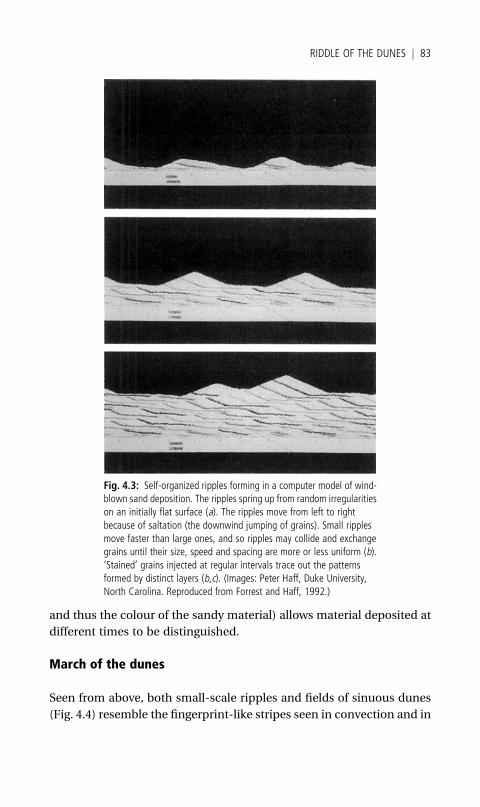
and thus the colour of the sandy material) allows material deposited at
different times to be distinguished.
March of the dunes
Seen from above, both small-scale ripples and fields of sinuous dunes
(Fig. 4.4) resemble the fingerprint-like stripes seen in convection and in
Fig. 4.3: Self-organized ripples forming in a computer model of wind-blown sand deposition. The ripples spring up from random irregularitieson an initially flat surface (a). The ripples move from left to rightbecause of saltation (the downwind jumping of grains). Small ripplesmove faster than large ones, and so ripples may collide and exchangegrains until their size, speed and spacing are more or less uniform (b).‘Stained’ grains injected at regular intervals trace out the patternsformed by distinct layers (b,c). (Images: Peter Haff, Duke University,North Carolina. Reproduced from Forrest and Haff, 1992.)
RIDDLE OF THE DUNES j 83
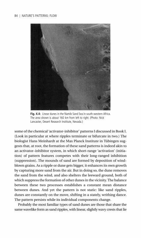
some of the chemical ‘activator-inhibitor’ patterns I discussed in Book I.
(Look in particular at where ripples terminate or bifurcate in two.) The
biologist Hans Meinhardt at the Max Planck Institute in Tubingen sug-
gests that, at root, the formation of these sand patterns is indeed akin to
an activator–inhibitor system, in which short-range ‘activation’ (initia-
tion) of pattern features competes with their long-ranged inhibition
(suppression). The mounds of sand are formed by deposition of wind-
blown grains. As a ripple or dune gets bigger, it enhances its own growth
by capturing more sand from the air. But in doing so, the dune removes
the sand from the wind, and also shelters the leeward ground, both of
which suppress the formation of other dunes in the vicinity. The balance
between these two processes establishes a constant mean distance
between dunes. And yet the pattern is not static: like sand ripples,
dunes are constantly on the move, shifting in a stately, writhing dance.
The pattern persists while its individual components change.
Probably the most familiar types of sand dunes are those that share the
samewavelike form as sand ripples, with linear, slightly wavy crests that lie
Fig. 4.4: Linear dunes in the Namib Sand Sea in south-western Africa.The area shown is about 160 km from left to right. (Photo: NickLancaster, Desert Research Institute, Nevada.)
84 j NATURE’S PATTERNS: FLOW
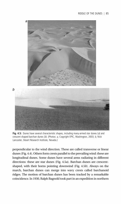
perpendicular to the wind direction. These are called transverse or linear
dunes (Fig. 4.4). Others formcrests parallel to theprevailingwind: these are
longitudinal dunes. Some dunes have several arms radiating in different
directions: these are star dunes (Fig. 4.5a). Barchan dunes are crescent-
shaped, with their horns pointing downwind (Fig. 4.5b). Always on the
march, barchan dunes can merge into wavy crests called barchanoid
ridges. The motion of barchan dunes has been tracked by a remarkable
coincidence. In 1930, RalphBagnold took part in an expedition in northern
Fig. 4.5: Dunes have several characteristic shapes, including many-armed star dunes (a) andcrescent shaped barchan dunes (b). (Photos: a, Copyright EPIC, Washington, 2003; b, NickLancaster, Desert Research Institute, Nevada.)
RIDDLE OF THE DUNES j 85
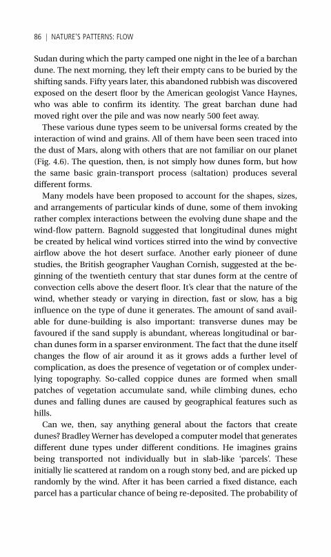
Sudan during which the party camped one night in the lee of a barchan
dune. The next morning, they left their empty cans to be buried by the
shifting sands. Fifty years later, this abandoned rubbish was discovered
exposed on the desert floor by the American geologist Vance Haynes,
who was able to confirm its identity. The great barchan dune had
moved right over the pile and was now nearly 500 feet away.
These various dune types seem to be universal forms created by the
interaction of wind and grains. All of them have been seen traced into
the dust of Mars, along with others that are not familiar on our planet
(Fig. 4.6). The question, then, is not simply how dunes form, but how
the same basic grain-transport process (saltation) produces several
different forms.
Many models have been proposed to account for the shapes, sizes,
and arrangements of particular kinds of dune, some of them invoking
rather complex interactions between the evolving dune shape and the
wind-flow pattern. Bagnold suggested that longitudinal dunes might
be created by helical wind vortices stirred into the wind by convective
airflow above the hot desert surface. Another early pioneer of dune
studies, the British geographer Vaughan Cornish, suggested at the be-
ginning of the twentieth century that star dunes form at the centre of
convection cells above the desert floor. It’s clear that the nature of the
wind, whether steady or varying in direction, fast or slow, has a big
influence on the type of dune it generates. The amount of sand avail-
able for dune-building is also important: transverse dunes may be
favoured if the sand supply is abundant, whereas longitudinal or bar-
chan dunes form in a sparser environment. The fact that the dune itself
changes the flow of air around it as it grows adds a further level of
complication, as does the presence of vegetation or of complex under-
lying topography. So-called coppice dunes are formed when small
patches of vegetation accumulate sand, while climbing dunes, echo
dunes and falling dunes are caused by geographical features such as
hills.
Can we, then, say anything general about the factors that create
dunes? Bradley Werner has developed a computer model that generates
different dune types under different conditions. He imagines grains
being transported not individually but in slab-like ‘parcels’. These
initially lie scattered at random on a rough stony bed, and are picked up
randomly by the wind. After it has been carried a fixed distance, each
parcel has a particular chance of being re-deposited. The probability of
86 j NATURE’S PATTERNS: FLOW
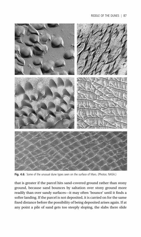
that is greater if the parcel hits sand-covered ground rather than stony
ground, because sand bounces by saltation over stony ground more
readily than over sandy surfaces—it may often ‘bounce’ until it finds a
softer landing. If the parcel is not deposited, it is carried on for the same
fixed distance before the possibility of being deposited arises again. If at
any point a pile of sand gets too steeply sloping, the slabs there slide
Fig. 4.6: Some of the unusual dune types seen on the surface of Mars. (Photos: NASA.)
RIDDLE OF THE DUNES j 87

downhill until the slope is stable. This maximum allowed slope of a
sand pile is called the angle of repose; we will see later that it plays a
major role in the behaviour of grainy materials.
Now, Werner’s model is not self-evidently a good way to describe
windblown sand: it seems a little odd to parcel up the sand into irre-
ducible slabs, for instance, or to assume that these always get carried
for the same distance before ‘hitting’ the ground again. Some of these
assumptions are understandable—dunes being so much bigger than
sand ripples, it’s not really feasible to simulate them grain by grain—but
that doesn’t mean they are reasonable. And yet the model seems to be
on to something, for with just these ingredients Werner was able to
reproduce all the major dune types: barchan, star, and linear dunes
(Fig. 4.7). When the wind was predominantly in a single direction,
dunes formed with their crests lying perpendicular to the wind (trans-
verse dunes), whereas if thewinddirectionwasmore variable, the dunes
were oriented in the average direction of the wind (longitudinal dunes).
While it is likely that specific, local influences affect dune sizes and
shapes, Werner’s model has the appealing feature that the broad pat-
terns that emerge are generic, not dependent on case-by-case details.
Within this picture, star and barchan dunes are as inevitable a feature of
nature’s tapestry as the branches of a river or the stripes of a zebra.
Hans Herrmann at the University of Stuttgart and his colleagues are
not convinced that dune formation is so simple. They say that some of
the dunes that appear to emerge from models like this are merely
transient structures, which will fade into a featureless bed of sand if
themodel is run for long enough. They think that the key factors in dune
Fig. 4.7: A model of dune formation devised by Bradley Werner generates many of the commondune types, including transverse and longitudinal linear dunes (a,b) and barchan dunes (c). Here Ishow the contours of the deposited material. The shapes depend on the wind direction andvariability, indicated by arrows. (Images: from Werner, 1995.)
88 j NATURE’S PATTERNS: FLOW
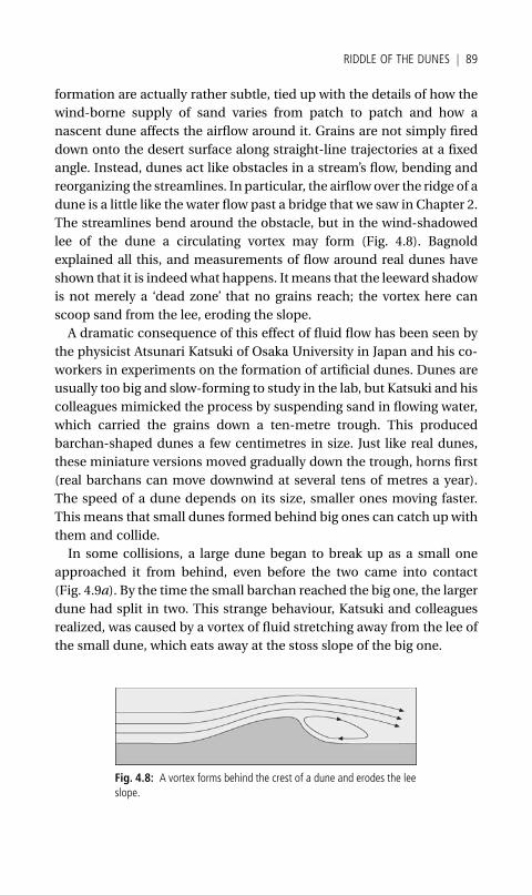
formation are actually rather subtle, tied up with the details of how the
wind-borne supply of sand varies from patch to patch and how a
nascent dune affects the airflow around it. Grains are not simply fired
down onto the desert surface along straight-line trajectories at a fixed
angle. Instead, dunes act like obstacles in a stream’s flow, bending and
reorganizing the streamlines. In particular, the airflow over the ridge of a
dune is a little like the water flow past a bridge that we saw in Chapter 2.
The streamlines bend around the obstacle, but in the wind-shadowed
lee of the dune a circulating vortex may form (Fig. 4.8). Bagnold
explained all this, and measurements of flow around real dunes have
shown that it is indeedwhat happens. It means that the leeward shadow
is not merely a ‘dead zone’ that no grains reach; the vortex here can
scoop sand from the lee, eroding the slope.
A dramatic consequence of this effect of fluid flow has been seen by
the physicist Atsunari Katsuki of Osaka University in Japan and his co-
workers in experiments on the formation of artificial dunes. Dunes are
usually too big and slow-forming to study in the lab, but Katsuki and his
colleagues mimicked the process by suspending sand in flowing water,
which carried the grains down a ten-metre trough. This produced
barchan-shaped dunes a few centimetres in size. Just like real dunes,
these miniature versions moved gradually down the trough, horns first
(real barchans can move downwind at several tens of metres a year).
The speed of a dune depends on its size, smaller ones moving faster.
This means that small dunes formed behind big ones can catch upwith
them and collide.
In some collisions, a large dune began to break up as a small one
approached it from behind, even before the two came into contact
(Fig. 4.9a). By the time the small barchan reached the big one, the larger
dune had split in two. This strange behaviour, Katsuki and colleagues
realized, was caused by a vortex of fluid stretching away from the lee of
the small dune, which eats away at the stoss slope of the big one.
Fig. 4.8: A vortex forms behind the crest of a dune and erodes the leeslope.
RIDDLE OF THE DUNES j 89
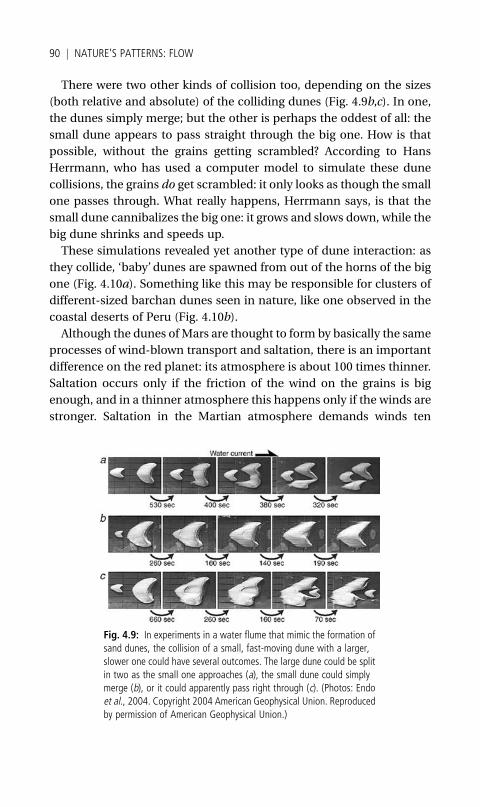
There were two other kinds of collision too, depending on the sizes
(both relative and absolute) of the colliding dunes (Fig. 4.9b,c). In one,
the dunes simply merge; but the other is perhaps the oddest of all: the
small dune appears to pass straight through the big one. How is that
possible, without the grains getting scrambled? According to Hans
Herrmann, who has used a computer model to simulate these dune
collisions, the grains do get scrambled: it only looks as though the small
one passes through. What really happens, Herrmann says, is that the
small dune cannibalizes the big one: it grows and slows down, while the
big dune shrinks and speeds up.
These simulations revealed yet another type of dune interaction: as
they collide, ‘baby’dunes are spawned from out of the horns of the big
one (Fig. 4.10a). Something like this may be responsible for clusters of
different-sized barchan dunes seen in nature, like one observed in the
coastal deserts of Peru (Fig. 4.10b).
Although the dunes ofMars are thought to form by basically the same
processes of wind-blown transport and saltation, there is an important
difference on the red planet: its atmosphere is about 100 times thinner.
Saltation occurs only if the friction of the wind on the grains is big
enough, and in a thinner atmosphere this happens only if the winds are
stronger. Saltation in the Martian atmosphere demands winds ten
Fig. 4.9: In experiments in a water flume that mimic the formation ofsand dunes, the collision of a small, fast-moving dune with a larger,slower one could have several outcomes. The large dune could be splitin two as the small one approaches (a), the small dune could simplymerge (b), or it could apparently pass right through (c). (Photos: Endoet al., 2004. Copyright 2004 American Geophysical Union. Reproducedby permission of American Geophysical Union.)
90 j NATURE’S PATTERNS: FLOW
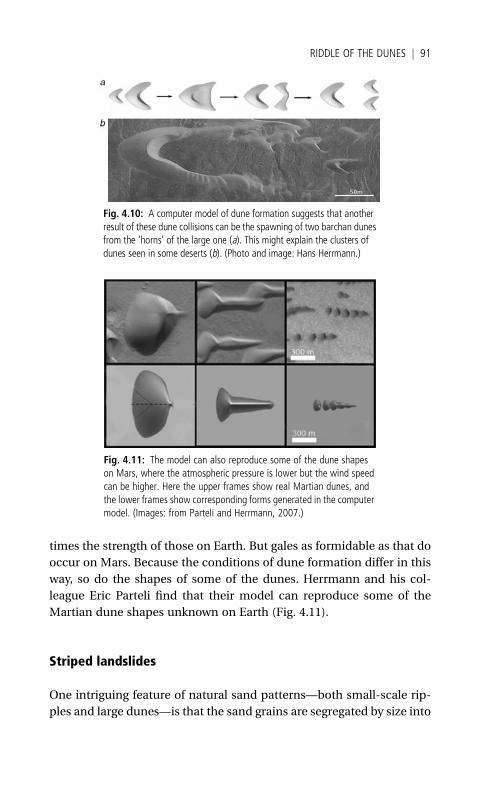
times the strength of those on Earth. But gales as formidable as that do
occur on Mars. Because the conditions of dune formation differ in this
way, so do the shapes of some of the dunes. Herrmann and his col-
league Eric Parteli find that their model can reproduce some of the
Martian dune shapes unknown on Earth (Fig. 4.11).
Striped landslides
One intriguing feature of natural sand patterns—both small-scale rip-
ples and large dunes—is that the sand grains are segregated by size into
Fig. 4.10: A computer model of dune formation suggests that anotherresult of these dune collisions can be the spawning of two barchan dunesfrom the ‘horns’ of the large one (a). This might explain the clusters ofdunes seen in some deserts (b). (Photo and image: Hans Herrmann.)
Fig. 4.11: The model can also reproduce some of the dune shapeson Mars, where the atmospheric pressure is lower but the wind speedcan be higher. Here the upper frames show real Martian dunes, andthe lower frames show corresponding forms generated in the computermodel. (Images: from Parteli and Herrmann, 2007.)
RIDDLE OF THE DUNES j 91
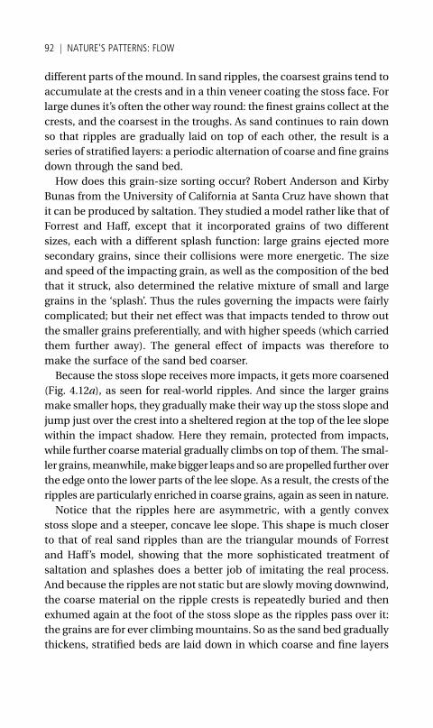
different parts of themound. In sand ripples, the coarsest grains tend to
accumulate at the crests and in a thin veneer coating the stoss face. For
large dunes it’s often the other way round: the finest grains collect at the
crests, and the coarsest in the troughs. As sand continues to rain down
so that ripples are gradually laid on top of each other, the result is a
series of stratified layers: a periodic alternation of coarse and fine grains
down through the sand bed.
How does this grain-size sorting occur? Robert Anderson and Kirby
Bunas from the University of California at Santa Cruz have shown that
it can be produced by saltation. They studied a model rather like that of
Forrest and Haff, except that it incorporated grains of two different
sizes, each with a different splash function: large grains ejected more
secondary grains, since their collisions were more energetic. The size
and speed of the impacting grain, as well as the composition of the bed
that it struck, also determined the relative mixture of small and large
grains in the ‘splash’. Thus the rules governing the impacts were fairly
complicated; but their net effect was that impacts tended to throw out
the smaller grains preferentially, and with higher speeds (which carried
them further away). The general effect of impacts was therefore to
make the surface of the sand bed coarser.
Because the stoss slope receives more impacts, it gets more coarsened
(Fig. 4.12a), as seen for real-world ripples. And since the larger grains
make smaller hops, they gradually make their way up the stoss slope and
jump just over the crest into a sheltered region at the top of the lee slope
within the impact shadow. Here they remain, protected from impacts,
while further coarsematerial gradually climbs on top of them. The smal-
ler grains,meanwhile,makebigger leaps and soarepropelled further over
the edge onto the lower parts of the lee slope. As a result, the crests of the
ripples are particularly enriched in coarse grains, again as seen in nature.
Notice that the ripples here are asymmetric, with a gently convex
stoss slope and a steeper, concave lee slope. This shape is much closer
to that of real sand ripples than are the triangular mounds of Forrest
and Haff’s model, showing that the more sophisticated treatment of
saltation and splashes does a better job of imitating the real process.
And because the ripples are not static but are slowlymoving downwind,
the coarse material on the ripple crests is repeatedly buried and then
exhumed again at the foot of the stoss slope as the ripples pass over it:
the grains are for ever climbingmountains. So as the sand bed gradually
thickens, stratified beds are laid down in which coarse and fine layers
92 j NATURE’S PATTERNS: FLOW
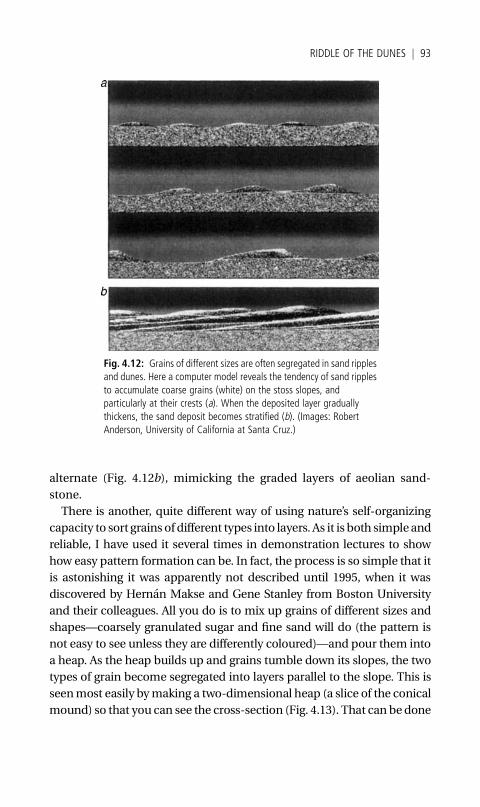
alternate (Fig. 4.12b), mimicking the graded layers of aeolian sand-
stone.
There is another, quite different way of using nature’s self-organizing
capacity to sort grains ofdifferent types into layers. As it is both simpleand
reliable, I have used it several times in demonstration lectures to show
how easy pattern formation can be. In fact, the process is so simple that it
is astonishing it was apparently not described until 1995, when it was
discovered by Hernan Makse and Gene Stanley from Boston University
and their colleagues. All you do is to mix up grains of different sizes and
shapes—coarsely granulated sugar and fine sand will do (the pattern is
not easy to see unless they are differently coloured)—and pour them into
a heap. As the heap builds up and grains tumble down its slopes, the two
types of grain become segregated into layers parallel to the slope. This is
seenmost easily bymaking a two-dimensional heap (a slice of the conical
mound) so that you can see the cross-section (Fig. 4.13). That can bedone
Fig. 4.12: Grains of different sizes are often segregated in sand ripplesand dunes. Here a computer model reveals the tendency of sand ripplesto accumulate coarse grains (white) on the stoss slopes, andparticularly at their crests (a). When the deposited layer graduallythickens, the sand deposit becomes stratified (b). (Images: RobertAnderson, University of California at Santa Cruz.)
RIDDLE OF THE DUNES j 93
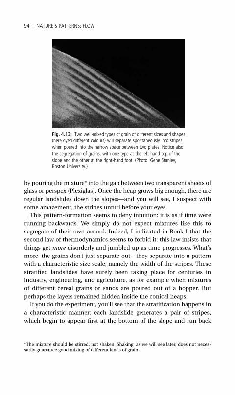
by pouring the mixture* into the gap between two transparent sheets of
glass or perspex (Plexiglas). Once the heap grows big enough, there are
regular landslides down the slopes—and you will see, I suspect with
some amazement, the stripes unfurl before your eyes.
This pattern-formation seems to deny intuition: it is as if time were
running backwards. We simply do not expect mixtures like this to
segregate of their own accord. Indeed, I indicated in Book I that the
second law of thermodynamics seems to forbid it: this law insists that
things get more disorderly and jumbled up as time progresses. What’s
more, the grains don’t just separate out—they separate into a pattern
with a characteristic size scale, namely the width of the stripes. These
stratified landslides have surely been taking place for centuries in
industry, engineering, and agriculture, as for example when mixtures
of different cereal grains or sands are poured out of a hopper. But
perhaps the layers remained hidden inside the conical heaps.
If you do the experiment, you’ll see that the stratification happens in
a characteristic manner: each landslide generates a pair of stripes,
which begin to appear first at the bottom of the slope and run back
*The mixture should be stirred, not shaken. Shaking, as we will see later, does not neces-
sarily guarantee good mixing of different kinds of grain.
Fig. 4.13: Two well-mixed types of grain of different sizes and shapes(here dyed different colours) will separate spontaneously into stripeswhen poured into the narrow space between two plates. Notice alsothe segregation of grains, with one type at the left-hand top of theslope and the other at the right-hand foot. (Photo: Gene Stanley,Boston University.)
94 j NATURE’S PATTERNS: FLOW
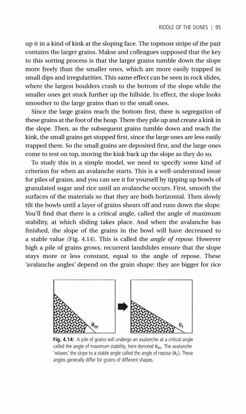
up it in a kind of kink at the sloping face. The topmost stripe of the pair
contains the larger grains. Makse and colleagues supposed that the key
to this sorting process is that the larger grains tumble down the slope
more freely than the smaller ones, which are more easily trapped in
small dips and irregularities. This same effect can be seen in rock slides,
where the largest boulders crash to the bottom of the slope while the
smaller ones get stuck further up the hillside. In effect, the slope looks
smoother to the large grains than to the small ones.
Since the large grains reach the bottom first, there is segregation of
these grains at the foot of the heap. There they pile up and create a kink in
the slope. Then, as the subsequent grains tumble down and reach the
kink, the small grains get stopped first, since the large ones are less easily
trapped there. So the small grains are deposited first, and the large ones
come to rest on top, moving the kink back up the slope as they do so.
To study this in a simple model, we need to specify some kind of
criterion for when an avalanche starts. This is a well-understood issue
for piles of grains, and you can see it for yourself by tipping up bowls of
granulated sugar and rice until an avalanche occurs. First, smooth the
surfaces of the materials so that they are both horizontal. Then slowly
tilt the bowls until a layer of grains shears off and runs down the slope.
You’ll find that there is a critical angle, called the angle of maximum
stability, at which sliding takes place. And when the avalanche has
finished, the slope of the grains in the bowl will have decreased to
a stable value (Fig. 4.14). This is called the angle of repose. However
high a pile of grains grows, recurrent landslides ensure that the slope
stays more or less constant, equal to the angle of repose. These
‘avalanche angles’ depend on the grain shape: they are bigger for rice
Fig. 4.14: A pile of grains will undergo an avalanche at a critical anglecalled the angle of maximum stability, here denoted um. The avalanche‘relaxes’ the slope to a stable angle called the angle of repose (ur). Theseangles generally differ for grains of different shapes.
RIDDLE OF THE DUNES j 95
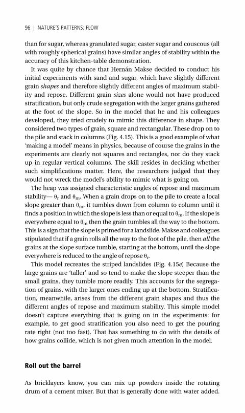
than for sugar, whereas granulated sugar, caster sugar and couscous (all
with roughly spherical grains) have similar angles of stability within the
accuracy of this kitchen-table demonstration.
It was quite by chance that Hernan Makse decided to conduct his
initial experiments with sand and sugar, which have slightly different
grain shapes and therefore slightly different angles of maximum stabil-
ity and repose. Different grain sizes alone would not have produced
stratification, but only crude segregation with the larger grains gathered
at the foot of the slope. So in the model that he and his colleagues
developed, they tried crudely to mimic this difference in shape. They
considered two types of grain, square and rectangular. These drop on to
the pile and stack in columns (Fig. 4.15). This is a good example of what
‘making a model’means in physics, because of course the grains in the
experiments are clearly not squares and rectangles, nor do they stack
up in regular vertical columns. The skill resides in deciding whether
such simplifications matter. Here, the researchers judged that they
would not wreck the model’s ability to mimic what is going on.
The heap was assigned characteristic angles of repose and maximum
stability— ur and um. When a grain drops on to the pile to create a local
slope greater than um, it tumbles down from column to column until it
finds a position inwhich the slope is less thanor equal to um. If the slope is
everywhere equal to um then the grain tumbles all the way to the bottom.
This is a sign that the slope is primed for a landslide.Makse andcolleagues
stipulated that if a grain rolls all theway to the foot of the pile, then all the
grains at the slope surface tumble, starting at the bottom, until the slope
everywhere is reduced to the angle of repose ur.
This model recreates the striped landslides (Fig. 4.15e) Because the
large grains are ‘taller’ and so tend to make the slope steeper than the
small grains, they tumble more readily. This accounts for the segrega-
tion of grains, with the larger ones ending up at the bottom. Stratifica-
tion, meanwhile, arises from the different grain shapes and thus the
different angles of repose and maximum stability. This simple model
doesn’t capture everything that is going on in the experiments: for
example, to get good stratification you also need to get the pouring
rate right (not too fast). That has something to do with the details of
how grains collide, which is not given much attention in the model.
Roll out the barrel
As bricklayers know, you can mix up powders inside the rotating
drum of a cement mixer. But that is generally done with water added.
96 j NATURE’S PATTERNS: FLOW
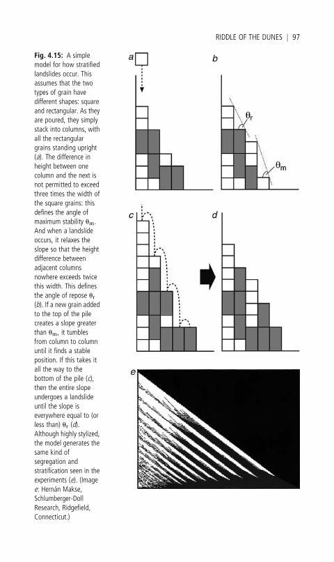
Fig. 4.15: A simplemodel for how stratifiedlandslides occur. Thisassumes that the twotypes of grain havedifferent shapes: squareand rectangular. As theyare poured, they simplystack into columns, withall the rectangulargrains standing upright(a). The difference inheight between onecolumn and the next isnot permitted to exceedthree times the width ofthe square grains: thisdefines the angle ofmaximum stability um.And when a landslideoccurs, it relaxes theslope so that the heightdifference betweenadjacent columnsnowhere exceeds twicethis width. This definesthe angle of repose ur(b). If a new grain addedto the top of the pilecreates a slope greaterthan um, it tumblesfrom column to columnuntil it finds a stableposition. If this takes itall the way to thebottom of the pile (c),then the entire slopeundergoes a landslideuntil the slope iseverywhere equal to (orless than) ur (d).Although highly stylized,the model generates thesame kind ofsegregation andstratification seen in theexperiments (e). (Imagee: Hernan Makse,Schlumberger-DollResearch, Ridgefield,Connecticut.)
RIDDLE OF THE DUNES j 97
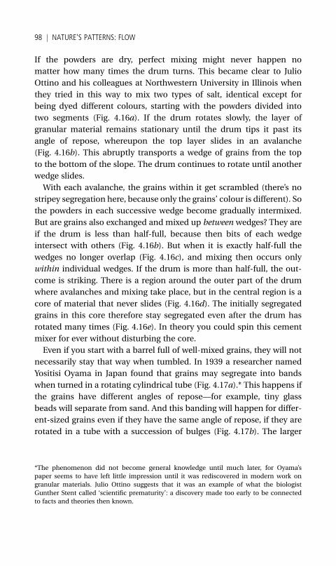
If the powders are dry, perfect mixing might never happen no
matter how many times the drum turns. This became clear to Julio
Ottino and his colleagues at Northwestern University in Illinois when
they tried in this way to mix two types of salt, identical except for
being dyed different colours, starting with the powders divided into
two segments (Fig. 4.16a). If the drum rotates slowly, the layer of
granular material remains stationary until the drum tips it past its
angle of repose, whereupon the top layer slides in an avalanche
(Fig. 4.16b). This abruptly transports a wedge of grains from the top
to the bottom of the slope. The drum continues to rotate until another
wedge slides.
With each avalanche, the grains within it get scrambled (there’s no
stripey segregation here, because only the grains’ colour is different). So
the powders in each successive wedge become gradually intermixed.
But are grains also exchanged and mixed up between wedges? They are
if the drum is less than half-full, because then bits of each wedge
intersect with others (Fig. 4.16b). But when it is exactly half-full the
wedges no longer overlap (Fig. 4.16c), and mixing then occurs only
within individual wedges. If the drum is more than half-full, the out-
come is striking. There is a region around the outer part of the drum
where avalanches and mixing take place, but in the central region is a
core of material that never slides (Fig. 4.16d). The initially segregated
grains in this core therefore stay segregated even after the drum has
rotated many times (Fig. 4.16e). In theory you could spin this cement
mixer for ever without disturbing the core.
Even if you start with a barrel full of well-mixed grains, they will not
necessarily stay that way when tumbled. In 1939 a researcher named
Yositisi Oyama in Japan found that grains may segregate into bands
when turned in a rotating cylindrical tube (Fig. 4.17a).* This happens if
the grains have different angles of repose—for example, tiny glass
beads will separate from sand. And this banding will happen for differ-
ent-sized grains even if they have the same angle of repose, if they are
rotated in a tube with a succession of bulges (Fig. 4.17b). The larger
*The phenomenon did not become general knowledge until much later, for Oyama’s
paper seems to have left little impression until it was rediscovered in modern work on
granular materials. Julio Ottino suggests that it was an example of what the biologist
Gunther Stent called ‘scientific prematurity’: a discovery made too early to be connected
to facts and theories then known.
98 j NATURE’S PATTERNS: FLOW
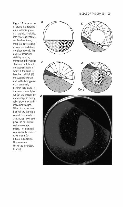
Fig. 4.16: Avalanchesof grains in a rotatingdrum will mix grainsthat are initially dividedinto two segments (a).As the drum turns,there is a succession ofavalanches each timethe slope exceeds theangle of maximumstability (b, c, d),transposing the wedgeshown in dark here tothe wedge shown inwhite. If the drum isless than half full (b),the wedges overlap,and so the two types ofgrain eventuallybecome fully mixed. Ifthe drum is exactly halffull (c), the wedges donot overlap, so mixingtakes place only withinindividual wedges.When it is more thanhalf full (d), there is acentral core in whichavalanches never takeplace, so this circularregion never getsmixed. This unmixedcore is clearly visible inexperiments (e).(Photo: Julio Ottino,NorthwesternUniversity, Evanston,Illinois.)
RIDDLE OF THE DUNES j 99
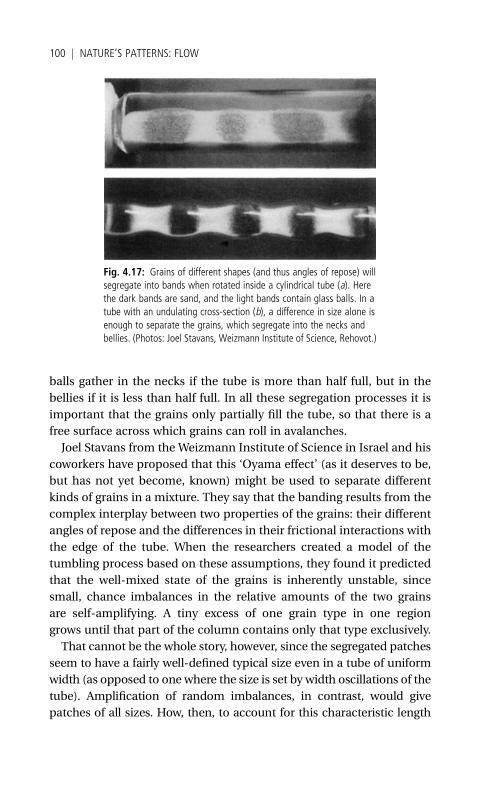
balls gather in the necks if the tube is more than half full, but in the
bellies if it is less than half full. In all these segregation processes it is
important that the grains only partially fill the tube, so that there is a
free surface across which grains can roll in avalanches.
Joel Stavans from the Weizmann Institute of Science in Israel and his
coworkers have proposed that this ‘Oyama effect’ (as it deserves to be,
but has not yet become, known) might be used to separate different
kinds of grains in a mixture. They say that the banding results from the
complex interplay between two properties of the grains: their different
angles of repose and the differences in their frictional interactions with
the edge of the tube. When the researchers created a model of the
tumbling process based on these assumptions, they found it predicted
that the well-mixed state of the grains is inherently unstable, since
small, chance imbalances in the relative amounts of the two grains
are self-amplifying. A tiny excess of one grain type in one region
grows until that part of the column contains only that type exclusively.
That cannot be the whole story, however, since the segregated patches
seem to have a fairly well-defined typical size even in a tube of uniform
width (as opposed to one where the size is set by width oscillations of the
tube). Amplification of random imbalances, in contrast, would give
patches of all sizes. How, then, to account for this characteristic length
Fig. 4.17: Grains of different shapes (and thus angles of repose) willsegregate into bands when rotated inside a cylindrical tube (a). Herethe dark bands are sand, and the light bands contain glass balls. In atube with an undulating cross-section (b), a difference in size alone isenough to separate the grains, which segregate into the necks andbellies. (Photos: Joel Stavans, Weizmann Institute of Science, Rehovot.)
100 j NATURE’S PATTERNS: FLOW
scale in the pattern? Stavans and colleagues point out that this is analo-
gous to what happens when a mixture of miscible (‘mixable’) fluids is
suddenly made immiscible (for example, by cooling them down). This
happens in rapid ‘quenching’ of a mixture of molten metals below their
freezing point: the twometals separate into blobs ofmore or less uniform
size. In this process, called spinodal decomposition, blobs of all sizes
grow in a self-amplifying manner, but those of a certain size are more
stable than the others and therefore get selected preferentially. By care-
fully controlling the conditions, such as the rate of cooling, a particular
blob size can be obtained by design; this is often done in metallurgy and
chemical engineering to make particles of specified sizes.
Self-organized avalanches
The problemwith landslides and avalanches is that you can never quite
be sure when they will happen. Sometimes they are set off by unpre-
dictable disturbances such as earthquakes—that is how most tsunamis
are generated, when seismic tremors send subsea sediments sliding
down a slope. But avalanches seem also to have an intrinsic capricious-
ness. For simple piles of more or less identical grains, we can feel sure
that there is trouble in store once the slope exceeds the angle of repose;
but even then it is hard to know how big the landslide will be. If the
grains are of many different sizes and shapes, or if they have complex
frictional properties (as is the case for wet soil or sticky snow crystals),
or if the surface on which they rest is rugged, we cannot be sure what to
expect. All we know is that when grains are set in motion, we had better
watch out.
Does that mean we can make no useful predictions about the timing
or the size of avalanches? Not exactly. Rather, it means that avalanche
science, like earthquake science, is necessarily statistical: we can’t say
exactly what will happen in a particular event, but we can know about
the relative probabilities of what might happen.
And in fact, studying landslides this way has proved to be astonish-
ingly productive. For it seems that the humble pile of sand is analogous
to a great many ‘catastrophic’ processes that happen in nature, from
forest fires to ecological mass extinctions. The key feature of all these
processes is that, while they are unpredictable, they are not fully
random in the sense that each event happens independently of the
RIDDLE OF THE DUNES j 101
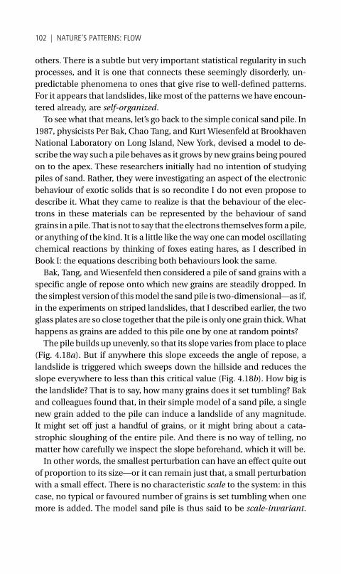
others. There is a subtle but very important statistical regularity in such
processes, and it is one that connects these seemingly disorderly, un-
predictable phenomena to ones that give rise to well-defined patterns.
For it appears that landslides, likemost of the patterns we have encoun-
tered already, are self-organized.
To see what thatmeans, let’s go back to the simple conical sand pile. In
1987, physicists Per Bak, Chao Tang, and Kurt Wiesenfeld at Brookhaven
National Laboratory on Long Island, New York, devised a model to de-
scribe theway such a pile behaves as it grows by new grains being poured
on to the apex. These researchers initially had no intention of studying
piles of sand. Rather, they were investigating an aspect of the electronic
behaviour of exotic solids that is so recondite I do not even propose to
describe it. What they came to realize is that the behaviour of the elec-
trons in these materials can be represented by the behaviour of sand
grains inapile. That is not to say that the electrons themselves formapile,
or anything of the kind. It is a little like theway one canmodel oscillating
chemical reactions by thinking of foxes eating hares, as I described in
Book I: the equations describing both behaviours look the same.
Bak, Tang, andWiesenfeld then considered a pile of sand grains with a
specific angle of repose onto which new grains are steadily dropped. In
the simplest versionof thismodel the sandpile is two-dimensional—as if,
in the experiments on striped landslides, that I described earlier, the two
glass plates are so close together that the pile is only one grain thick.What
happens as grains are added to this pile one by one at random points?
The pile builds up unevenly, so that its slope varies fromplace to place
(Fig. 4.18a). But if anywhere this slope exceeds the angle of repose, a
landslide is triggered which sweeps down the hillside and reduces the
slope everywhere to less than this critical value (Fig. 4.18b). How big is
the landslide? That is to say, how many grains does it set tumbling? Bak
and colleagues found that, in their simple model of a sand pile, a single
new grain added to the pile can induce a landslide of any magnitude.
It might set off just a handful of grains, or it might bring about a cata-
strophic sloughing of the entire pile. And there is no way of telling, no
matter how carefully we inspect the slope beforehand, which it will be.
In other words, the smallest perturbation can have an effect quite out
of proportion to its size—or it can remain just that, a small perturbation
with a small effect. There is no characteristic scale to the system: in this
case, no typical or favoured number of grains is set tumbling when one
more is added. The model sand pile is thus said to be scale-invariant.
102 j NATURE’S PATTERNS: FLOW
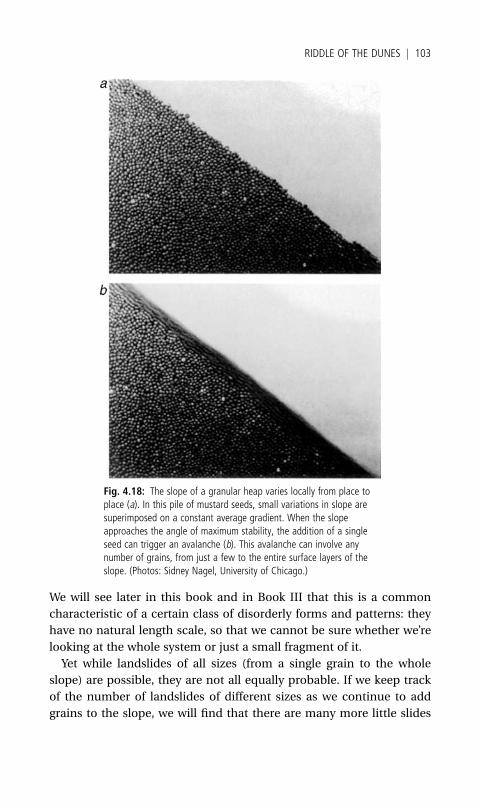
We will see later in this book and in Book III that this is a common
characteristic of a certain class of disorderly forms and patterns: they
have no natural length scale, so that we cannot be sure whether we’re
looking at the whole system or just a small fragment of it.
Yet while landslides of all sizes (from a single grain to the whole
slope) are possible, they are not all equally probable. If we keep track
of the number of landslides of different sizes as we continue to add
grains to the slope, we will find that there are many more little slides
Fig. 4.18: The slope of a granular heap varies locally from place toplace (a). In this pile of mustard seeds, small variations in slope aresuperimposed on a constant average gradient. When the slopeapproaches the angle of maximum stability, the addition of a singleseed can trigger an avalanche (b). This avalanche can involve anynumber of grains, from just a few to the entire surface layers of theslope. (Photos: Sidney Nagel, University of Chicago.)
RIDDLE OF THE DUNES j 103
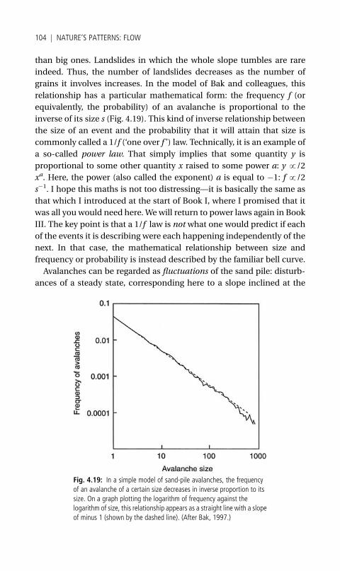
than big ones. Landslides in which the whole slope tumbles are rare
indeed. Thus, the number of landslides decreases as the number of
grains it involves increases. In the model of Bak and colleagues, this
relationship has a particular mathematical form: the frequency f (or
equivalently, the probability) of an avalanche is proportional to the
inverse of its size s (Fig. 4.19). This kind of inverse relationship between
the size of an event and the probability that it will attain that size is
commonly called a 1/f (‘one over f ’) law. Technically, it is an example of
a so-called power law. That simply implies that some quantity y is
proportional to some other quantity x raised to some power a: y !/2
xa. Here, the power (also called the exponent) a is equal to �1: f !/2
s�1. I hope this maths is not too distressing—it is basically the same as
that which I introduced at the start of Book I, where I promised that it
was all you would need here. We will return to power laws again in Book
III. The key point is that a 1/f law is not what one would predict if each
of the events it is describing were each happening independently of the
next. In that case, the mathematical relationship between size and
frequency or probability is instead described by the familiar bell curve.
Avalanches can be regarded as fluctuations of the sand pile: disturb-
ances of a steady state, corresponding here to a slope inclined at the
Fig. 4.19: In a simple model of sand-pile avalanches, the frequencyof an avalanche of a certain size decreases in inverse proportion to itssize. On a graph plotting the logarithm of frequency against thelogarithm of size, this relationship appears as a straight line with a slopeof minus 1 (shown by the dashed line). (After Bak, 1997.)
104 j NATURE’S PATTERNS: FLOW
angle of repose. If we added no more grains to such a slope, it would
remain unchanging indefinitely. When we do add grains, the slope has a
continual series of convulsions (avalanches) of all sizes, all of which
rearrange the slope so that on average it rests at the angle of repose. The
constant rain of grains makes the sand pile a non-equilibrium system.
We encountered these in Book I, where I explained that they are the
sources of most natural patterns. We also saw there that, in order to
keep a system out of equilibrium, we have to provide a constant supply
of energy, and generally of matter too. That is what is happening to the
sand pile: the falling grains are perpetually injecting energy and matter
into the slope. This is what drives the fluctuations.
It turns out that 1/f laws govern the size of fluctuations observed in
a wide variety of natural and human-made systems. An electrical cur-
rent flowing through a resistor undergoes tiny fluctuations of this kind,
and so does the amount of heat and light (the luminosity) emitted by
the Sun. These latter fluctuations are due to outbursts of super-hot
plasma called solar flares, which are generated by writhing magnetic
fields in the Sun’s outer atmosphere. The light fromdistant astrophysical
objects called quasars shows the same kind of variability; so do some
records of volcanic eruptions and of rainfall. Some palaeontologists
have argued that the geological record ofmass extinctions (catastrophic
events that wipe out a significant fraction of organisms on Earth)
seem also to show a 1/f relationship between the size and frequency of
the events, at least for marine ecosystems. In all these cases, we can
see abrupt avalanche-like events happening on all size scales.
Although 1/f power laws have long been known to govern the statis-
tical behaviour of fluctuations in diverse natural systems, the reasons
for it were unknown before Per Bak and his colleagues devised their
model of a sand pile. Here, then, was a simple instance of such behav-
iour, in which all the ingredients were known, that might offer some
clues about the general origin of 1/f laws.
There is something very peculiar about this model sand pile: it is
constantly seeking the least stable state. We are used to quite the
opposite: nature generally seems to crave stability, which is why water
runs downhill, golf balls drop into holes, trees topple. The sand pile,
however, is for ever returning to the state in which it is poised on the
brink of an avalanche. Each time an avalanche occurs, this precarious
balancing act gives way; but then as further grains are added, the
system creeps right back to the brink.
RIDDLE OF THE DUNES j 105

States like this, which are susceptible to fluctuations on all scales at
the slightest provocation, have been known to physicists for a long
time. They are called critical states, and are found in systems as diverse
as magnets, liquids, and theoretical models of the Big Bang. Every
liquid adopts a critical state at a particular temperature and pressure,
called the critical point. If you heat a liquid, it evaporates to a vapour
once it reaches boiling point: the state of the fluid changes abruptly
from a (dense) liquid to a (rarefied) gas. But above the critical tempera-
ture this abrupt change of state no longer happens; instead, the fluid
passes smoothly and continuously from a dense liquid-like state to a
diffuse gas-like state as its pressure is lowered. The critical point is the
point at which there is no longer any sharp distinction between ‘liquid’
and ‘gas’, and no boiling point separating the two.
At the critical point of a fluid, its density fluctuates wildly from one
place to another (Fig. 4.20). In some patches the fluid has a liquid-like
density, in others it is gas-like, and these patches are constantly chan-
Fig. 4.20: At thecritical point of a liquidand a gas, thedistinction betweenthese two states ofmatter disappears. Acritical fluid containsvariations in density onall scales, with domainsof liquid-like fluidcoexisting with domainsof gas-like fluid. Here Ishow a snapshot of sucha fluid, obtained from acomputer model of acritical point. The darkregions represent liquid-like, dense domains, andthe white regions aregas-like. (Image: AlastairBruce, University ofEdinburgh.)
106 j NATURE’S PATTERNS: FLOW
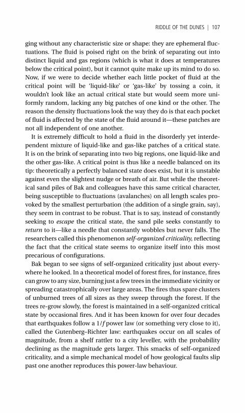
ging without any characteristic size or shape: they are ephemeral fluc-
tuations. The fluid is poised right on the brink of separating out into
distinct liquid and gas regions (which is what it does at temperatures
below the critical point), but it cannot quite make up its mind to do so.
Now, if we were to decide whether each little pocket of fluid at the
critical point will be ‘liquid-like’ or ‘gas-like’ by tossing a coin, it
wouldn’t look like an actual critical state but would seem more uni-
formly random, lacking any big patches of one kind or the other. The
reason the density fluctuations look the way they do is that each pocket
of fluid is affected by the state of the fluid around it—these patches are
not all independent of one another.
It is extremely difficult to hold a fluid in the disorderly yet interde-
pendent mixture of liquid-like and gas-like patches of a critical state.
It is on the brink of separating into two big regions, one liquid-like and
the other gas-like. A critical point is thus like a needle balanced on its
tip: theoretically a perfectly balanced state does exist, but it is unstable
against even the slightest nudge or breath of air. But while the theoret-
ical sand piles of Bak and colleagues have this same critical character,
being susceptible to fluctuations (avalanches) on all length scales pro-
voked by the smallest perturbation (the addition of a single grain, say),
they seem in contrast to be robust. That is to say, instead of constantly
seeking to escape the critical state, the sand pile seeks constantly to
return to it—like a needle that constantly wobbles but never falls. The
researchers called this phenomenon self-organized criticality, reflecting
the fact that the critical state seems to organize itself into this most
precarious of configurations.
Bak began to see signs of self-organized criticality just about every-
where he looked. In a theoretical model of forest fires, for instance, fires
can grow to any size, burning just a few trees in the immediate vicinity or
spreading catastrophically over large areas. The fires thus spare clusters
of unburned trees of all sizes as they sweep through the forest. If the
trees re-grow slowly, the forest is maintained in a self-organized critical
state by occasional fires. And it has been known for over four decades
that earthquakes follow a 1/f power law (or something very close to it),
called the Gutenberg–Richter law: earthquakes occur on all scales of
magnitude, from a shelf rattler to a city leveller, with the probability
declining as the magnitude gets larger. This smacks of self-organized
criticality, and a simple mechanical model of how geological faults slip
past one another reproduces this power-law behaviour.
RIDDLE OF THE DUNES j 107
Per Bak believed that in self-organized criticality he had uncovered ‘a
comprehensive framework to describe the ubiquity of complexity in
Nature’—and not just in nature but in human systems too, such as the
fluctuations of economic markets and the spread of technological
innovation. There is no doubt that many of the models developed to
describe complex systems of this sort do find their way into a self-
organized critical state. But verifying that the real world also behaves
that way is much harder, and many of the claimed instances of self-
organized criticality, such as inmass extinctions and forest fires, remain
contentious. One of the problems is that the statistics are often am-
biguous. To be sure you are seeing a particular kind of mathematical
relationship between size and frequency, and not just something that
looks a bit like it over a small range of size scales, you need a lot of
data—which you can’t always get. There may not have been enough
mass extinctions since the beginning of the world, for example, to allow
us to be sure that evolution operates in a self-organized critical state.
Another problem is that, whereas in a model you can usually be sure
exactly what all the important parameters are, and can see the effect of
changing each one independently, in reality complex systems may be
susceptible to all manner of perturbing influences, some more obvious
than others. Will a model of earthquake faulting that includes a more
realistic description of the sliding process or of the geological structure
of the Earth still show self-organized criticality?
In fact, it is even contentiouswhether real sandpiles, the inspiration for
the original model, have self-organized critical states. Youmight imagine
that this, at least, ought to be a simple experiment to perform: you just
drop sand grain by grain on to a pile and observe how big an avalanche
follows from each addition. But there is no unique way to measure the
size of an avalanche, and the experiments that have been conducted so
far do not give a clear answer. For example, Sidney Nagel and his col-
leagues at the University of Chicago found in 1989 that real sand piles
seem always to undergo large avalanches, in which most of the top layer
of sand slides away, while other experiments in the early 1990s seemed to
generate power-law behaviour like that expected of self-organized critic-
ality.Many researchers now think that real sand piles don’t show true self-
organized criticality; but it is also possible that it is subtly disguised so
that it doesn’t show up in the measured size of avalanches.
If sand piles are not really self-organized critical states, perhaps that is
not so surprising, since real sand is not like model sand. For one thing,
the grains are not identical in size, shape or surface features, and these
108 j NATURE’S PATTERNS: FLOW
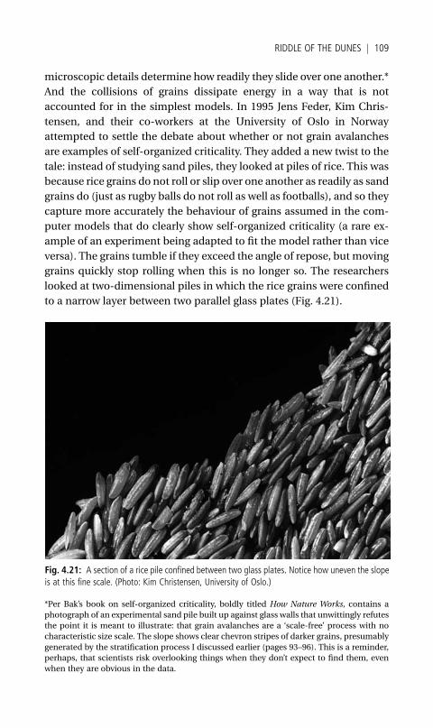
microscopic details determine how readily they slide over one another.*
And the collisions of grains dissipate energy in a way that is not
accounted for in the simplest models. In 1995 Jens Feder, Kim Chris-
tensen, and their co-workers at the University of Oslo in Norway
attempted to settle the debate about whether or not grain avalanches
are examples of self-organized criticality. They added a new twist to the
tale: instead of studying sand piles, they looked at piles of rice. This was
because rice grains do not roll or slip over one another as readily as sand
grains do (just as rugby balls do not roll as well as footballs), and so they
capture more accurately the behaviour of grains assumed in the com-
puter models that do clearly show self-organized criticality (a rare ex-
ample of an experiment being adapted to fit the model rather than vice
versa). The grains tumble if they exceed the angle of repose, but moving
grains quickly stop rolling when this is no longer so. The researchers
looked at two-dimensional piles in which the rice grains were confined
to a narrow layer between two parallel glass plates (Fig. 4.21).
Fig. 4.21: A section of a rice pile confined between two glass plates. Notice how uneven the slopeis at this fine scale. (Photo: Kim Christensen, University of Oslo.)
*Per Bak’s book on self-organized criticality, boldly titled How Nature Works, contains a
photograph of an experimental sand pile built up against glass walls that unwittingly refutes
the point it is meant to illustrate: that grain avalanches are a ‘scale-free’ process with no
characteristic size scale. The slope shows clear chevron stripes of darker grains, presumably
generated by the stratification process I discussed earlier (pages 93–96). This is a reminder,
perhaps, that scientists risk overlooking things when they don’t expect to find them, even
when they are obvious in the data.
RIDDLE OF THE DUNES j 109

Observing enough avalanches to provide trustworthy statistics was a
slow and tedious process, and took about a year. But at the end of it all,
the researchers concluded that the behaviour of these granular piles
depended on the kind of rice that they used: specifically, on whether it
was long grain or short grain. Long-grain rice with a larger ratio of
length to width seems to show true self-organized critical behaviour,
with a power-law relationship between the size of the avalanche (the
researchers actually measured how much energy each one released)
and its frequency of occurrence. But short-grain rice, which is more
nearly spherical and so more like sand, showed different behaviour:
instead of a simple power law, the relationship between size and fre-
quency was more complicated than a 1/f law. That relationship could,
however, be easily mistaken for a power law (and thus for the signature
of self-organized criticality) if the measurements were not taken over a
wide enough range of avalanche sizes, possibly explaining why others
had previously claimed to have seen self-organized criticality in experi-
mental sand piles.
So, while piles of grains apparently can show self-organized behaviour,
theywillnotnecessarily doso, and indeedgenerallywillnot; it dependson
(amongst other things) the shape of the grains and how their energy is
dissipated during tumbling. This both vindicates and modifies Bak’s
assertions: self-organized criticality seems to be a real phenomenon, not
just a product of computer models, but it may not be universal or even
particularly easy to observe or achieve. For the present time, sand piles
appear to be an intriguing but limited metaphor for nature’s complexity.
The rise or fall of nuts
I am not very good at using up the last of a packet of muesli. It is
dreadfully wasteful, I know, but the fact is that by the time you get to
the bottom, all the large pieces of fruit and nuts are gone and all that’s
left is a rather unappetizing residue of dry oat flakes. The big pieces
always seem to stay on top, and the small ones settle to the bottom.
This has become known to physicists as the Brazil nut effect.
The sorting of grains of different sizes in a shaken granular medium is
well known to engineers, but the reason for it is still disputed. You
might think that shaking would simply mix up grains of different
sizes, but clearly this is not so—usually, the larger grains instead rise
110 j NATURE’S PATTERNS: FLOW
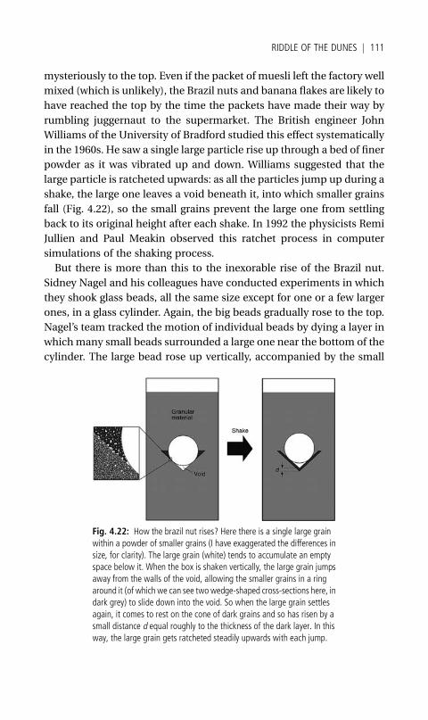
mysteriously to the top. Even if the packet of muesli left the factory well
mixed (which is unlikely), the Brazil nuts and banana flakes are likely to
have reached the top by the time the packets have made their way by
rumbling juggernaut to the supermarket. The British engineer John
Williams of the University of Bradford studied this effect systematically
in the 1960s. He saw a single large particle rise up through a bed of finer
powder as it was vibrated up and down. Williams suggested that the
large particle is ratcheted upwards: as all the particles jump up during a
shake, the large one leaves a void beneath it, into which smaller grains
fall (Fig. 4.22), so the small grains prevent the large one from settling
back to its original height after each shake. In 1992 the physicists Remi
Jullien and Paul Meakin observed this ratchet process in computer
simulations of the shaking process.
But there is more than this to the inexorable rise of the Brazil nut.
Sidney Nagel and his colleagues have conducted experiments in which
they shook glass beads, all the same size except for one or a few larger
ones, in a glass cylinder. Again, the big beads gradually rose to the top.
Nagel’s team tracked the motion of individual beads by dying a layer in
whichmany small beads surrounded a large one near the bottom of the
cylinder. The large bead rose up vertically, accompanied by the small
Fig. 4.22: How the brazil nut rises? Here there is a single large grainwithin a powder of smaller grains (I have exaggerated the differences insize, for clarity). The large grain (white) tends to accumulate an emptyspace below it. When the box is shaken vertically, the large grain jumpsaway from the walls of the void, allowing the smaller grains in a ringaround it (of which we can see two wedge-shaped cross-sections here, indark grey) to slide down into the void. So when the large grain settlesagain, it comes to rest on the cone of dark grains and so has risen by asmall distance d equal roughly to the thickness of the dark layer. In thisway, the large grain gets ratcheted steadily upwards with each jump.
RIDDLE OF THE DUNES j 111
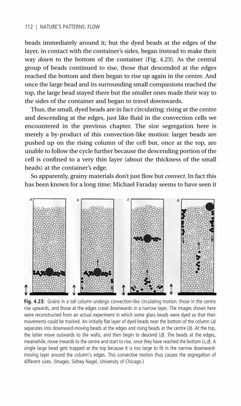
beads immediately around it; but the dyed beads at the edges of the
layer, in contact with the container’s sides, began instead to make their
way down to the bottom of the container (Fig. 4.23). As the central
group of beads continued to rise, those that descended at the edges
reached the bottom and then began to rise up again in the centre. And
once the large bead and its surrounding small companions reached the
top, the large bead stayed there but the smaller ones made their way to
the sides of the container and began to travel downwards.
Thus, the small, dyed beads are in fact circulating: rising at the centre
and descending at the edges, just like fluid in the convection cells we
encountered in the previous chapter. The size segregation here is
merely a by-product of this convection-like motion: larger beads are
pushed up on the rising column of the cell but, once at the top, are
unable to follow the cycle further because the descending portion of the
cell is confined to a very thin layer (about the thickness of the small
beads) at the container’s edge.
So apparently, grainy materials don’t just flow but convect. In fact this
has been known for a long time; Michael Faraday seems to have seen it
Fig. 4.23: Grains in a tall column undergo convection-like circulating motion: those in the centrerise upwards, and those at the edges crawl downwards in a narrow layer. The images shown herewere reconstructed from an actual experiment in which some glass beads were dyed so that theirmovements could be tracked. An initially flat layer of dyed beads near the bottom of the column (a)separates into downward-moving beads at the edges and rising beads at the centre (b). At the top,the latter move outwards to the walls, and then begin to descend (d). The beads at the edges,meanwhile, move inwards to the centre and start to rise, once they have reached the bottom (c,d). Asingle large bead gets trapped at the top because it is too large to fit in the narrow downward-moving layer around the column’s edges. This convective motion thus causes the segregation ofdifferent sizes. (Images: Sidney Nagel, University of Chicago.)
112 j NATURE’S PATTERNS: FLOW
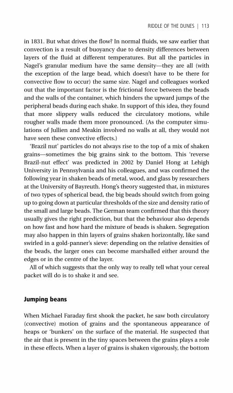
in 1831. But what drives the flow? In normal fluids, we saw earlier that
convection is a result of buoyancy due to density differences between
layers of the fluid at different temperatures. But all the particles in
Nagel’s granular medium have the same density—they are all (with
the exception of the large bead, which doesn’t have to be there for
convective flow to occur) the same size. Nagel and colleagues worked
out that the important factor is the frictional force between the beads
and the walls of the container, which hinders the upward jumps of the
peripheral beads during each shake. In support of this idea, they found
that more slippery walls reduced the circulatory motions, while
rougher walls made them more pronounced. (As the computer simu-
lations of Jullien and Meakin involved no walls at all, they would not
have seen these convective effects.)
‘Brazil nut’ particles do not always rise to the top of a mix of shaken
grains—sometimes the big grains sink to the bottom. This ‘reverse
Brazil-nut effect’ was predicted in 2002 by Daniel Hong at Lehigh
University in Pennsylvania and his colleagues, and was confirmed the
following year in shaken beads of metal, wood, and glass by researchers
at the University of Bayreuth. Hong’s theory suggested that, in mixtures
of two types of spherical bead, the big beads should switch from going
up to going down at particular thresholds of the size and density ratio of
the small and large beads. The German team confirmed that this theory
usually gives the right prediction, but that the behaviour also depends
on how fast and how hard the mixture of beads is shaken. Segregation
may also happen in thin layers of grains shaken horizontally, like sand
swirled in a gold-panner’s sieve: depending on the relative densities of
the beads, the larger ones can become marshalled either around the
edges or in the centre of the layer.
All of which suggests that the only way to really tell what your cereal
packet will do is to shake it and see.
Jumping beans
When Michael Faraday first shook the packet, he saw both circulatory
(convective) motion of grains and the spontaneous appearance of
heaps or ‘bunkers’ on the surface of the material. He suspected that
the air that is present in the tiny spaces between the grains plays a role
in these effects. When a layer of grains is shaken vigorously, the bottom
RIDDLE OF THE DUNES j 113
of the layer jumps away from the floor, creating a cavity that contains
almost no air. The abrupt difference in air pressure between the gas
amongst the grains and this almost air-free cavity pushes some grains
underneath the pile as it rises, and so creates unevenness in the layer,
leading to heaping. By performed experiments in which the pressure of
the gas permeating the granular layer is changed systematically to
investigate the effect on heaping, researchers have recently confirmed
Faraday’s mechanism.
Faraday proposed it as an explanation for the patterns seen in vibrat-
ing grains by the eighteenth-century German physicist Ernst Chladni.
Chladni found in 1787 that if fine sand is scattered over a metal plate
and the edge of the plate is bowed with a violin bow to excite an
acoustic vibration, the powder gathers into lines and spots that inter-
weave in rather beautiful patterns (Fig. 4.24). The vibrations of the plate
depend on how they are excited: how hard, and at what frequency. Like
a kind of two-dimensional organ pipe or guitar string, the plate has
particular ‘modes’ of vibration in which whole numbers of waves fit
perfectly onto the surface. As with a guitar string, some points of the
vibrating surface will bemoving upwards while other parts move down-
wards, and at some point in between there is a so-called node where the
surface doesn’t move at all (Fig. 4.25). On a plucked string this node is a
single point, but on a plate it can trace out a line. Chladni noted that
fine particles and coarse particles sitting on the surface behave differ-
ently: the fine ones pile up at the ‘antinodes’, where the plate has the
maximum amplitude of up-down motion, while the coarse ones gather
at nodes where there is no plate motion. Faraday suggested that, while
the big grains just jump about until they reach the points on the surface
that aren’t moving, the fine particles are pushed to the antinodes by air
currents caused by the pressure differences induced as the layer jumps
and opens up cavities. He tested this by sticking pieces of paper to the
plates to block or channel the air flow, and found that these had the
expected effect of redirecting the grains. Surprisingly, Faraday’s general
idea did not receive clear experimental support until 1998.
His theory suggests that the behaviour of a layer of vibrated grains
should depend on the air pressure above it. In the mid-1900s, Harry
Swinney and colleagues Paul Umbanhowar and Francisco Melo at the
University of Texas at Austin decided to see what happens to a shaken
layer of grains when there is no air at all, and thus no air currents. They
studied a very thin layer of tiny bronze spheres, each about the same size
114 j NATURE’S PATTERNS: FLOW
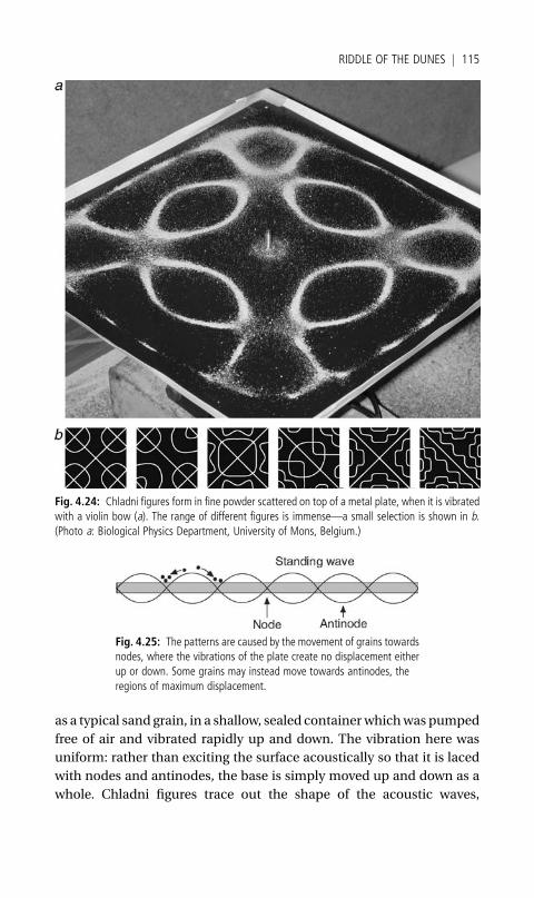
as a typical sand grain, in a shallow, sealed container whichwas pumped
free of air and vibrated rapidly up and down. The vibration here was
uniform: rather than exciting the surface acoustically so that it is laced
with nodes and antinodes, the base is simply moved up and down as a
whole. Chladni figures trace out the shape of the acoustic waves,
Fig. 4.24: Chladni figures form in fine powder scattered on top of a metal plate, when it is vibratedwith a violin bow (a). The range of different figures is immense—a small selection is shown in b.(Photo a: Biological Physics Department, University of Mons, Belgium.)
Fig. 4.25: The patterns are caused by the movement of grains towardsnodes, where the vibrations of the plate create no displacement eitherup or down. Some grains may instead move towards antinodes, theregions of maximum displacement.
RIDDLE OF THE DUNES j 115
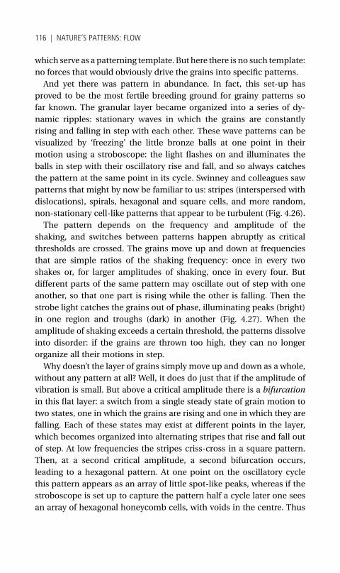
which serve as a patterning template. But here there is no such template:
no forces that would obviously drive the grains into specific patterns.
And yet there was pattern in abundance. In fact, this set-up has
proved to be the most fertile breeding ground for grainy patterns so
far known. The granular layer became organized into a series of dy-
namic ripples: stationary waves in which the grains are constantly
rising and falling in step with each other. These wave patterns can be
visualized by ‘freezing’ the little bronze balls at one point in their
motion using a stroboscope: the light flashes on and illuminates the
balls in step with their oscillatory rise and fall, and so always catches
the pattern at the same point in its cycle. Swinney and colleagues saw
patterns that might by now be familiar to us: stripes (interspersed with
dislocations), spirals, hexagonal and square cells, and more random,
non-stationary cell-like patterns that appear to be turbulent (Fig. 4.26).
The pattern depends on the frequency and amplitude of the
shaking, and switches between patterns happen abruptly as critical
thresholds are crossed. The grains move up and down at frequencies
that are simple ratios of the shaking frequency: once in every two
shakes or, for larger amplitudes of shaking, once in every four. But
different parts of the same pattern may oscillate out of step with one
another, so that one part is rising while the other is falling. Then the
strobe light catches the grains out of phase, illuminating peaks (bright)
in one region and troughs (dark) in another (Fig. 4.27). When the
amplitude of shaking exceeds a certain threshold, the patterns dissolve
into disorder: if the grains are thrown too high, they can no longer
organize all their motions in step.
Why doesn’t the layer of grains simply move up and down as a whole,
without any pattern at all? Well, it does do just that if the amplitude of
vibration is small. But above a critical amplitude there is a bifurcation
in this flat layer: a switch from a single steady state of grain motion to
two states, one in which the grains are rising and one in which they are
falling. Each of these states may exist at different points in the layer,
which becomes organized into alternating stripes that rise and fall out
of step. At low frequencies the stripes criss-cross in a square pattern.
Then, at a second critical amplitude, a second bifurcation occurs,
leading to a hexagonal pattern. At one point on the oscillatory cycle
this pattern appears as an array of little spot-like peaks, whereas if the
stroboscope is set up to capture the pattern half a cycle later one sees
an array of hexagonal honeycomb cells, with voids in the centre. Thus
116 j NATURE’S PATTERNS: FLOW
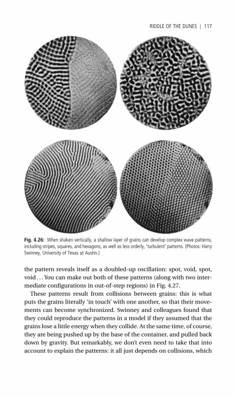
the pattern reveals itself as a doubled-up oscillation: spot, void, spot,
void . . . You can make out both of these patterns (along with two inter-
mediate configurations in out-of-step regions) in Fig. 4.27.
These patterns result from collisions between grains: this is what
puts the grains literally ‘in touch’ with one another, so that their move-
ments can become synchronized. Swinney and colleagues found that
they could reproduce the patterns in a model if they assumed that the
grains lose a little energy when they collide. At the same time, of course,
they are being pushed up by the base of the container, and pulled back
down by gravity. But remarkably, we don’t even need to take that into
account to explain the patterns: it all just depends on collisions, which
Fig. 4.26: When shaken vertically, a shallow layer of grains can develop complex wave patterns,including stripes, squares, and hexagons, as well as less orderly, ‘turbulent’ patterns. (Photos: HarrySwinney, University of Texas at Austin.)
RIDDLE OF THE DUNES j 117
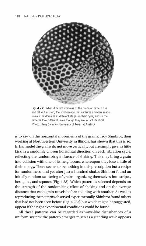
is to say, on the horizontal movements of the grains. Troy Shinbrot, then
working at Northwestern University in Illinois, has shown that this is so.
In hismodel the grains do notmove vertically, but are simply given a little
kick in a randomly chosen horizontal direction on each vibration cycle,
reflecting the randomizing influence of shaking. This may bring a grain
into collision with one of its neighbours, whereupon they lose a little of
their energy. There seems to be nothing in this prescription but a recipe
for randomness, and yet after just a hundred shakes Shinbrot found an
initially random scattering of grains organizing themselves into stripes,
hexagons, and squares (Fig. 4.28). Which pattern is selected depends on
the strength of the randomizing effect of shaking and on the average
distance that each grain travels before colliding with another. As well as
reproducing the patterns observed experimentally, Shinbrot foundothers
that had not been seen before (Fig. 4.28d) but whichmight, he suggested,
appear if the right experimental conditions could be found.
All these patterns can be regarded as wave-like disturbances of a
uniform system: the pattern emerges much as a standing wave appears
Fig. 4.27: When different domains of the granular pattern riseand fall out of step, the stroboscope that captures a frozen imagereveals the domains at different stages in their cycle, and so thepatterns look different, even though they are in fact identical.(Photo: Harry Swinney, University of Texas at Austin.)
118 j NATURE’S PATTERNS: FLOW

in a vibrated tray of water.* But there is another way in which we can
describe them: as ranks of individual elements that interact with each
other to form ordered structures, like people arranging themselves
evenly spaced out on a crowded beach. You could regard this picture
as a kind of ‘particle-like’ alternative to the wave-like picture of global
instabilities with characteristic wavelengths. It is possible to capture
Fig. 4.28: Complex ordered and irregular patterns arise spontaneously in a simple model of ashaken thin layer of grains as a result of the interplay between random ‘noisiness’ of the grainmovements and collisions between them. (Images: Troy Shinbrot, Northwestern University,Evanston, Illinois.)
*This is more metaphor than analogy. A standing wave has its wavelength set by the size of
the container: the wave has to ‘fit’. But the regular patterns in vibrated grains are more
striking because the wavelength is determined by the properties of the grains themselves: by
how they collide, and how far theymove between collisions. This is why these latter are truly
self-organized patterns.
RIDDLE OF THE DUNES j 119
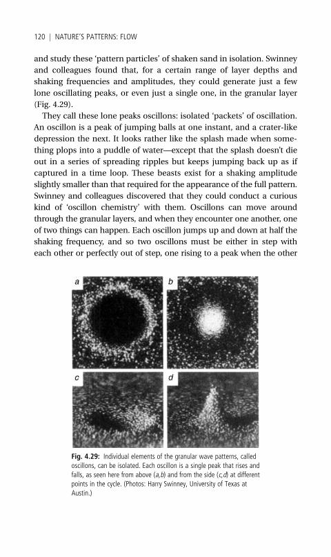
and study these ‘pattern particles’ of shaken sand in isolation. Swinney
and colleagues found that, for a certain range of layer depths and
shaking frequencies and amplitudes, they could generate just a few
lone oscillating peaks, or even just a single one, in the granular layer
(Fig. 4.29).
They call these lone peaks oscillons: isolated ‘packets’ of oscillation.
An oscillon is a peak of jumping balls at one instant, and a crater-like
depression the next. It looks rather like the splash made when some-
thing plops into a puddle of water—except that the splash doesn’t die
out in a series of spreading ripples but keeps jumping back up as if
captured in a time loop. These beasts exist for a shaking amplitude
slightly smaller than that required for the appearance of the full pattern.
Swinney and colleagues discovered that they could conduct a curious
kind of ‘oscillon chemistry’ with them. Oscillons can move around
through the granular layers, and when they encounter one another, one
of two things can happen. Each oscillon jumps up and down at half the
shaking frequency, and so two oscillons must be either in step with
each other or perfectly out of step, one rising to a peak when the other
Fig. 4.29: Individual elements of the granular wave patterns, calledoscillons, can be isolated. Each oscillon is a single peak that rises andfalls, as seen here from above (a,b) and from the side (c,d) at differentpoints in the cycle. (Photos: Harry Swinney, University of Texas atAustin.)
120 j NATURE’S PATTERNS: FLOW
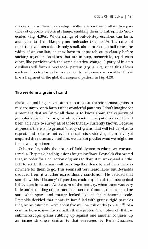
makes a crater. Two out-of-step oscillons attract each other, like par-
ticles of opposite electrical charge, enabling them to link up into ‘mol-
ecules’ (Fig. 4.30a). Whole strings of out-of-step oscillons can form,
analogous to chain-like polymer molecules (Fig. 4.30b). The range of
the attractive interaction is only small, about one and a half times the
width of an oscillon, so they have to approach quite closely before
sticking together. Oscillons that are in step, meanwhile, repel each
other, like particles with the same electrical charge. A party of in-step
oscillons will form a hexagonal pattern (Fig. 4.30c), since this allows
each oscillon to stay as far from all of its neighbours as possible. This is
like a fragment of the global hexagonal pattern in Fig. 4.26.
The world in a grain of sand
Shaking, tumbling or even simple pouring can therefore cause grains to
mix, to unmix, or to form rather wonderful patterns. I don’t imagine for
a moment that we know all there is to know about the capacity of
granular substances for generating spontaneous patterns, nor have I
been able here to survey all of those that are currently known. Because
at present there is no general ‘theory of grains’ that will tell us what to
expect, and because not even the scientists studying them have yet
acquired the necessary intuition, we cannot predict what we might see
in a given experiment.
Osborne Reynolds, the doyen of fluid dynamics whom we encoun-
tered in Chapter 2, had big visions for grainy flows. Reynolds discovered
that, in order for a collection of grains to flow, it must expand a little.
Left to settle, the grains will pack together densely, and then there is
nowhere for them to go. This seems all very reasonable, but Reynolds
deduced from it a rather extraordinary conclusion. He decided that
somehow this ‘dilatancy’ of powders could explain all the mechanical
behaviours in nature. At the turn of the century, when there was very
little understanding of the internal structure of atoms, no one could be
sure what space and matter looked like at the subatomic scale.
Reynolds decided that it was in fact filled with grains: rigid particles
that, by his estimate, were about five million-trillionths (5 � 10�18) of a
centimetre across—much smaller than a proton. The notion of all these
submicroscopic grains rubbing up against one another conjures up
an image strikingly similar to that envisaged by Rene Descartes
RIDDLE OF THE DUNES j 121
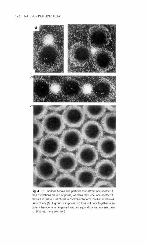
Fig. 4.30: Oscillons behave like particles that attract one another iftheir oscillations are out of phase, whereas they repel one another ifthey are in phase. Out-of-phase oscillons can form ‘oscillon molecules’(a) or chains (b). A group of in-phase oscillons will pack together in anorderly, hexagonal arrangement with an equal distance between them(c). (Photos: Harry Swinney.)
122 j NATURE’S PATTERNS: FLOW
in the seventeenth century, who postulated a universe filled with vor-
tices in contact. Descartes’s fluid, you might say, became Reynolds’s
powder.
His idea was rather eccentric even by the standards of Victorian
science. John Collier’s portrait of Reynolds from 1904 shows him hold-
ing a basin of ball-bearings, and in a prestigious lecture two years
earlier he revealed what he had in mind with this seemingly innocuous
collection of hard particles: ‘I have in my hand the first experimental
model universe, a soft India rubber bag filled with small shot.’ Blake’s
phrase is invoked to the point of cliche in research on grainy materials,
but for Reynolds it became a reality.
RIDDLE OF THE DUNES j 123
5Follow Your NeighbourFlocks, Swarms, and Crowds
IONCE saw the Harvard biologist E. O. Wilson asked a challenging
question by a nervous young man at a public lecture. Wilson won a
Pulitzer prize in 1990 for a book written with fellow naturalist Bert
Holldobler on the behaviour of ants—a definitive and weighty tome, yet
communicated with joy and passion. But honestly, the young man
exclaimed with awkward and genuine puzzlement, how could a person
spend their entire research career studying something as straightfor-
ward, as prosaic and, let’s face it, as small as ants?
Wilson is by no means famous only for his work on ants. As a leading
proponent of sociobiology, otherwise known as evolutionary psych-
ology, he became notorious in the 1970s for his endorsement of what
some considered (wrongly) to be a rigidly deterministic view of human
nature with right-wing overtones. Nonetheless, his enthusiasm for ants
runs very deep, and the audience was perceptibly anxious at how
Wilson might receive this apparently naive dismissal. But there was
no hint of condescension or defensiveness in his answer. He simply
suggested to the young man that he scatter some sugar near an ant’s
nest on a warm day—and then sit back and watch. What will unfold, he
implied, will soon seem an appropriate subject for a life’s work.
You could say much the same about many other organisms. Sit in a
park at dusk and watch a group of swallows dive and swoop, and you
enter into a profound mystery. Watch schools of fish evading their
predators off the Great Barrier Reef, or herds of wildebeest crossing
the savannah, or even observe a culture of bacteria proliferate and
spread under a microscope, and you begin to understand that bio-
logical organization does not stop at the level of the individual organ-
ism. All these groups display motions that hint at some grand scheme,
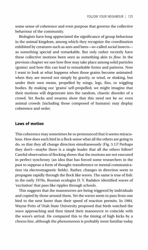
some sense of coherence and even purpose that governs the collective
behaviour of the community.
Biologists have long appreciated the significance of group behaviour
in the animal kingdom, among which they recognize the coordination
exhibited by creatures such as ants and bees—so-called social insects—
as something special and remarkable. But only rather recently have
these collective motions been seen as something akin to flow. In the
previous chapter we saw how flowmay take place among solid particles
(grains) and how this can lead to remarkable forms and patterns. Now
I want to look at what happens when those grains become animated:
when they are moved not simply by gravity, or wind, or shaking, but
under their own steam, propelled by wings, legs, fins, or wiggling
bodies. By making our ‘grains’ self-propelled, we might imagine that
their motions will degenerate into the random, chaotic disorder of a
crowd. Yet flocks and swarms show that this need not be so: even
animal crowds (including those composed of humans) may display
coherence and order.
Laws of motion
This coherencemay sometimes be so pronounced that it seemsmiracu-
lous. How does each bird in a flock sense what all the others are going to
do, so that they all change direction simultaneously (Fig. 5.1)? Perhaps
they don’t—maybe there is a single leader that all the others follow?
Careful observation of flocking shows that themotions are not executed
in perfect synchrony (an idea that has forced some researchers in the
past to suppose a form of thought-transference or mental communica-
tion via electromagnetic fields). Rather, changes in direction seem to
propagate rapidly through the flock like waves. The same is true of fish:
in the early 1970s, Russian ecologist D. V. Radakov identified waves of
‘excitation’ that pass like ripples through schools.
This suggests that the manoeuvres are being triggered by individuals
and copied by those around them. Yet the waves seem to pass from one
bird to the next faster than their speed of reaction permits. In 1984,
Wayne Potts of Utah State University proposed that birds watched the
wave approaching and then timed their manoeuvre to coincide with
the wave’s arrival. He compared this to the timing of high kicks by a
chorus line, although the phenomenon is probably more familiar today
FOLLOW YOUR NEIGHBOUR j 125
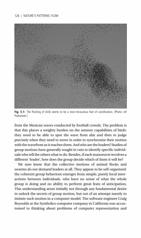
from the Mexican waves conducted by football crowds. The problem is
that this places a weighty burden on the sensory capabilities of birds:
they need to be able to spot the wave from afar and then to judge
precisely when they need to move in order to synchronize their motion
with thewavefront as it reaches them.Andwhoare the leaders? Studiesof
groupmotions have generally sought in vain to identify specific individ-
ualswho tell the otherswhat to do. Besides, if eachmanoeuvre involves a
different ‘leader’, how does the group decide which of them it will be?
We now know that the collective motions of animal flocks and
swarms do not demand leaders at all. They appear to be self-organized:
the coherent group behaviour emerges from simple, purely local inter-
actions between individuals, who have no sense of what the whole
group is doing and no ability to perform great feats of anticipation.
This understanding arose initially not through any fundamental desire
to unlock the secrets of group motion, but out of an attempt merely to
imitate such motion in a computer model. The software engineer Craig
Reynolds at the Symbolics computer company in California was accus-
tomed to thinking about problems of computer representation and
Fig. 5.1: The flocking of birds seems to be a near-miraculous feat of coordination. (Photo: JefPoskanzer.)
126 j NATURE’S PATTERNS: FLOW
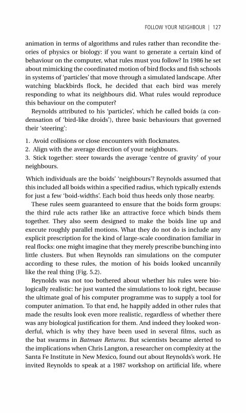
animation in terms of algorithms and rules rather than recondite the-
ories of physics or biology: if you want to generate a certain kind of
behaviour on the computer, what rules must you follow? In 1986 he set
aboutmimicking the coordinatedmotion of bird flocks and fish schools
in systems of ‘particles’ that move through a simulated landscape. After
watching blackbirds flock, he decided that each bird was merely
responding to what its neighbours did. What rules would reproduce
this behaviour on the computer?
Reynolds attributed to his ‘particles’, which he called boids (a con-
densation of ‘bird-like droids’), three basic behaviours that governed
their ‘steering’:
1. Avoid collisions or close encounters with flockmates.
2. Align with the average direction of your neighbours.
3. Stick together: steer towards the average ‘centre of gravity’ of your
neighbours.
Which individuals are the boids’ ‘neighbours’? Reynolds assumed that
this included all boids within a specified radius, which typically extends
for just a few ‘boid-widths’. Each boid thus heeds only those nearby.
These rules seem guaranteed to ensure that the boids form groups:
the third rule acts rather like an attractive force which binds them
together. They also seem designed to make the boids line up and
execute roughly parallel motions. What they do not do is include any
explicit prescription for the kind of large-scale coordination familiar in
real flocks: onemight imagine that theymerely prescribe bunching into
little clusters. But when Reynolds ran simulations on the computer
according to these rules, the motion of his boids looked uncannily
like the real thing (Fig. 5.2).
Reynolds was not too bothered about whether his rules were bio-
logically realistic: he just wanted the simulations to look right, because
the ultimate goal of his computer programme was to supply a tool for
computer animation. To that end, he happily added in other rules that
made the results look even more realistic, regardless of whether there
was any biological justification for them. And indeed they looked won-
derful, which is why they have been used in several films, such as
the bat swarms in Batman Returns. But scientists became alerted to
the implications when Chris Langton, a researcher on complexity at the
Santa Fe Institute in New Mexico, found out about Reynolds’s work. He
invited Reynolds to speak at a 1987 workshop on artificial life, where
FOLLOW YOUR NEIGHBOUR j 127
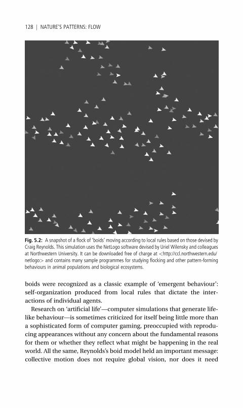
boids were recognized as a classic example of ‘emergent behaviour’:
self-organization produced from local rules that dictate the inter-
actions of individual agents.
Research on ‘artificial life’—computer simulations that generate life-
like behaviour—is sometimes criticized for itself being little more than
a sophisticated form of computer gaming, preoccupied with reprodu-
cing appearances without any concern about the fundamental reasons
for them or whether they reflect what might be happening in the real
world. All the same, Reynolds’s boid model held an important message:
collective motion does not require global vision, nor does it need
Fig. 5.2: A snapshot of a flock of ‘boids’ moving according to local rules based on those devised byCraig Reynolds. This simulation uses the NetLogo software devised by Uriel Wilensky and colleaguesat Northwestern University. It can be downloaded free of charge at <http://ccl.northwestern.edu/netlogo> and contains many sample programmes for studying flocking and other pattern-formingbehaviours in animal populations and biological ecosystems.
128 j NATURE’S PATTERNS: FLOW
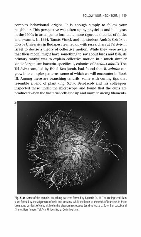
complex behavioural origins. It is enough simply to follow your
neighbour. This perspective was taken up by physicists and biologists
in the 1990s in attempts to formulate more rigorous theories of flocks
and swarms. In 1994, Tamas Vicsek and his student Andras Czirok at
Eotvos University in Budapest teamed upwith researchers at Tel Aviv in
Israel to devise a theory of collective motion. While they were aware
that their model might have something to say about birds and fish, its
primary motive was to explain collective motion in a much simpler
kind of organism: bacteria, specifically colonies of Bacillus subtilis. The
Tel Aviv team, led by Eshel Ben-Jacob, had found that B. subtilis can
grow into complex patterns, some of which we will encounter in Book
III. Among these are branching tendrils, some with curling tips that
resemble a kind of plant (Fig. 5.3a). Ben-Jacob and his colleagues
inspected these under the microscope and found that the curls are
produced when the bacterial cells line up andmove in arcing filaments.
Fig. 5.3: Some of the complex branching patterns formed by bacteria (a, b). The curling tendrils ina are formed by the alignment of cells into streams, while the blobs at the ends of branches in b arecirculating vortices of cells, visible in the electron microscope (c). (Photos: a,b: Eshel Ben-Jacob andKineret Ben Knaan, Tel Aviv University; c, Colin Ingham.)
FOLLOW YOUR NEIGHBOUR j 129
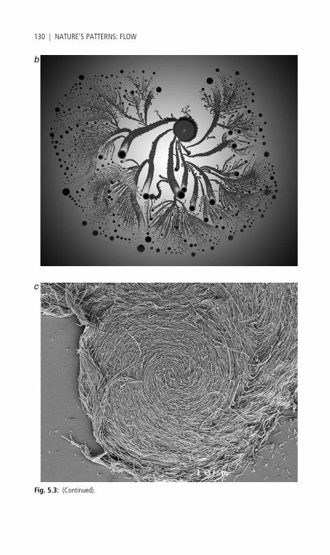
Fig. 5.3: (Continued).
130 j NATURE’S PATTERNS: FLOW
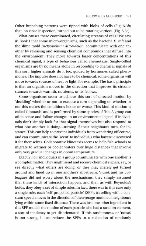
Other branching patterns were tipped with blobs of cells (Fig. 5.3b)
that, on close inspection, turned out to be rotating vortices (Fig. 5.3c).
What causes these coordinated, circulating streams of cells? We saw
in Book I that some micro-organisms, such as the bacteria E. coli and
the slime mold Dictyostelium discoideum, communicate with one an-
other by releasing and sensing chemical compounds that diffuse into
the environment. They move towards larger concentrations of this
chemical signal, a type of behaviour called chemotaxis. Single-celled
organisms are by no means alone in responding to chemical signals of
this sort: higher animals do it too, guided by hormones called phero-
mones. The impulse does not have to be chemical: some organisms will
move towards sources of heat or light, for example. The basic principle
is that an organism moves in the direction that improves its circum-
stances: towards warmth, nutrients, or its fellows.
Some organisms seem to achieve this sort of directed motion by
‘deciding’ whether or not to execute a turn depending on whether or
not this makes the conditions better or worse. This kind of motion is
called klinotaxis, and is performed by some species of fish. A group can
often sense and follow changes in an environmental signal if individ-
uals don’t simply look for that signal themselves but also respond to
what one another is doing—turning if their neighbours turn, for in-
stance. This can help to prevent individuals from wandering off course,
and can communicate the ‘scent’ to individuals who haven’t discovered
it for themselves. Collaborative klinotaxis seems to help fish schools to
migrate to warmer or cooler waters over huge distances that involve
only very gradual changes in ocean temperature.
Exactly how individuals in a group communicate with one another is
a complexmatter. Theymight send and receive chemical signals, say, or
see directly what others are doing, or they may merely get turned
around and lined up in one another’s slipstream. Vicsek and his col-
leagues did not worry about the mechanisms; they simply assumed
that these kinds of interaction happen, and that, as with Reynolds’s
boids, they obey a set of simple rules. In fact, there was in this case only
a single rule: each ‘self-propelled particle’ (SPP), travelling with a con-
stant speed, moves in the direction of the averagemotion of neighbours
lying within some fixed distance. There was just one other ingredient in
this SPPmodel: themotion of each particle also had a random element,
a sort of tendency to get disorientated. If this randomness, or ‘noise’,
is too strong, it can reduce the SPPs to a collection of randomly
FOLLOW YOUR NEIGHBOUR j 131
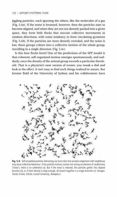
jiggling particles, each ignoring the others, like the molecules of a gas
(Fig. 5.4a). If the noise is lessened, however, then the particles start to
become aligned, and when they are not too densely packed into a given
space, they form little flocks that execute collective movements in
random directions, with some tendency to form circulating gyrations
(Fig. 5.4b). If the particles are more densely crowded, and the noise is
low, these groups cohere into a collective motion of the whole group,
travelling in a single direction (Fig. 5.4c).
Is this how flocks form? One of the predictions of the SPP model is
that coherent, self-organized motion emerges spontaneously, and sud-
denly, once the density of the animal group exceeds a particular thresh-
old. That is a physicist’s neat version of events: you tweak a dial and
look at the effect. It isn’t easy to find such things realized in nature. But
Jerome Buhl of the University of Sydney and his collaborators have
Fig. 5.4: Self-propelled particles interacting via local rules that produce alignment with neighboursmay show collective behaviour. If the particle motions contain too strong an element of randomness(‘noise’), there is no coherence (a). But if the noise is reduced, the particles gather into alignedbunches (b), or, if their density is large enough, all stream together in a single direction (c). (Images:Tamas Vicsek, Eotvos Lorand University, Budapest.)
132 j NATURE’S PATTERNS: FLOW
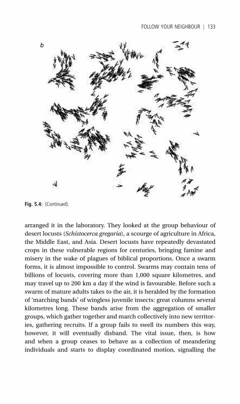
arranged it in the laboratory. They looked at the group behaviour of
desert locusts (Schistocerca gregaria), a scourge of agriculture in Africa,
the Middle East, and Asia. Desert locusts have repeatedly devastated
crops in these vulnerable regions for centuries, bringing famine and
misery in the wake of plagues of biblical proportions. Once a swarm
forms, it is almost impossible to control. Swarms may contain tens of
billions of locusts, covering more than 1,000 square kilometres, and
may travel up to 200 km a day if the wind is favourable. Before such a
swarm of mature adults takes to the air, it is heralded by the formation
of ‘marching bands’ of wingless juvenile insects: great columns several
kilometres long. These bands arise from the aggregation of smaller
groups, which gather together and march collectively into new territor-
ies, gathering recruits. If a group fails to swell its numbers this way,
however, it will eventually disband. The vital issue, then, is how
and when a group ceases to behave as a collection of meandering
individuals and starts to display coordinated motion, signalling the
Fig. 5.4: (Continued).
FOLLOW YOUR NEIGHBOUR j 133
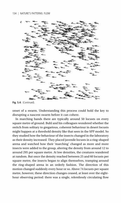
onset of a swarm. Understanding this process could hold the key to
disrupting a nascent swarm before it can cohere.
In marching bands there are typically around 50 locusts on every
squaremetre of ground. Buhl and his colleagues wondered whether the
switch from solitary to gregarious, coherent behaviour in desert locusts
might happen at a threshold density like that seen in the SPP model. So
they studied how the behaviour of the insects changed in the laboratory
as their density increased. They placed juvenile locusts in a ring-shaped
arena and watched how their ‘marching’ changed as more and more
insects were added to the group, altering the density from around 12 to
around 295 per square metre. At low densities, the creatures wandered
at random. But once the density reached between 25 and 60 locusts per
square metre, the insects began to align themselves, tramping around
the ring-shaped arena in an orderly fashion. The direction of this
motion changed suddenly every hour or so. Above 74 locusts per square
metre, however, these direction changes ceased, at least over the eight-
hour observing period: there was a single, relentlessly circulating flow
Fig. 5.4: (Continued).
134 j NATURE’S PATTERNS: FLOW
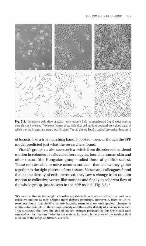
of locusts, like a true marching band. It looked, then, as though the SPP
model predicted just what the researchers found.
Vicsek’s group has also seen such a switch from disordered to ordered
motion in colonies of cells called keratocytes, found in human skin and
other tissues (the Hungarian group studied those of goldfish scales).
These cells are able to move across a surface—that is how they gather
together in the right places to form tissues. Vicsek and colleagues found
that as the density of cells increased, they saw a change from random
motion to collective, vortex-like motions and finally to coherent flow of
the whole group, just as seen in the SPP model (Fig. 5.5).*
*It’s not clear that mobile single cells will always show these sharp switches from random to
collective motion as they become more densely populated, however. A team of US re-
searchers found that Bacillus subtilis bacteria seem to show only gradual changes in
motion—for example, in the average velocity of cells—as the density of a colony increased.
They suspected that here the kind of sudden changes predicted by the SPP model were
smeared out by random ‘noise’ in the system, for example because of the swirling fluid
medium or the range of different cell sizes.
Fig. 5.5: Keratocyte cells show a switch from random (left) to coordinated (right) movement astheir density increases. The lower images show individual cell motions deduced from video data, ofwhich the top images are snapshots. (Images: Tamas Vicsek, Eotvos Lorand University, Budapest.)
FOLLOW YOUR NEIGHBOUR j 135
Group memory
The SPP model has its limitations. For one thing, it doesn’t rule out
collisions between the ‘particles’, whereas real creatures seek to avoid
bumping into one another. Nor does the model have any ingredient for
forming groups that stay permanently together: it can generate little
swarms that form and reform, and it can make all the particles in the
box move as one, but it does not explain how a group such as a fish
school can hold together without any box to contain it.
Iain Couzin of Princeton University and his co-workers have tried to
correct these deficits, while looking at motions in three-dimensional
space rather than just two. The local rules governing the behaviour of
their particles are more complicated, but they are biologically reason-
able. Each individual is surrounded by concentric, spherical zones of
interaction, which determine the creature’s behaviour when another
individual enters one of these zones (Fig. 5.6a). Very close to the
individual there is a zone of repulsion: when a neighbour enters this
zone, the creature will perform an avoidance manoeuvre to ensure they
don’t collide. Beyond this there is a zone of orientation: when other
individuals come within this zone, the creature will aim to align its
motion with the average of theirs. And beyond that is a zone of attrac-
tion: the creature will simply try to stay close to others within this zone,
without bothering about orientation. It prioritizes these rules, so that,
for example, it will forget about orientation and concentrate on colli-
sion-avoidance if there are any individuals in the zone of repulsion.
Exactly how a group of simulated creatures behaves in any particular
case depends on all the various ingredients of the model, such as how
dense the group is, how big the zones of interaction are, how fast the
creatures move, and so forth. But even though these offer countless
permutations of the model ‘settings’, there are just four different basic
types of behaviour that emerge (Fig. 5.6b–e). One is a group that holds
together but without otherwise any coherence of motion. This is like a
swarm of insects such as gnats, buzzing about at random in a dense
cloud. Then there is a group that moves hither and thither in approxi-
mate alignment, reminiscent of a bird flock or fish school. The group
might alternatively display highly regimented motion in a single direc-
tion, like a group of migrating birds. And finally, the group may circu-
late together in a doughnut or torus shape. This last might seem odd
and artificial, but in fact it is rather common: some fish, for example
behave this way (Fig. 5.7a). Certain species of fish have to keep moving
136 j NATURE’S PATTERNS: FLOW

Fig. 5.6: In the model of collective animal motion devised by IainCouzin and his co-workers, each individual moves in a manner thattakes into account the presence of others in three nested sphericalzones (a). The innermost zone is repulsive: the creature will aim toavoid others that come this close. But it will orientate its motion withthe average of others inside the second zone. And it will merely try tostay close to others within the outermost zone of attraction. Fourdifferent types of group behaviour emerge from these rules (b–e). Thegroup may cluster without any orientational alignment, in a swarm (b).Or the motions may be aligned, like a flock or school (c). Or it may allmove in a single direction (d), or circulate in a hoop (e). (After Couzinand Krause, 2002.)
FOLLOW YOUR NEIGHBOUR j 137
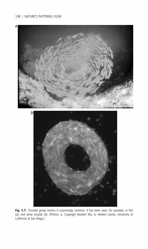
Fig. 5.7: Toroidal group motion is surprisingly common. It has been seen, for example, in fish(a), and slime moulds (b). (Photos: a, Copyright Norbert Wu; b, Herbert Levine, University ofCalifornia at San Diego.)
138 j NATURE’S PATTERNS: FLOW
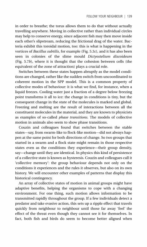
in order to breathe; the torus allows them to do that without actually
travelling anywhere. Moving in collective rather than individual circles
may help to conserve energy, since adjacent fish may then move inside
each other’s slipstream, reducing the frictional drag of the water. Bac-
teria exhibit this toroidal motion, too: this is what is happening in the
vortices of Bacillus subtilis, for example (Fig. 5.3c), and it has also been
seen in colonies of the slime mould Dictyostelium discoideum
(Fig. 5.7b), where it is thought that the cohesion between cells (the
equivalent of the zone of attraction) plays a crucial role.
Switches between these states happen abruptly as the model condi-
tions are changed, rather like the sudden switch from uncoordinated to
coherent motion in the SPP model. This is a common property of
collective modes of behaviour: it is what we find, for instance, when a
liquid freezes. Cooling water just a fraction of a degree below freezing
point transforms it all to ice: the change in conditions is tiny, but the
consequent change in the state of the molecules is marked and global.
Freezing and melting are the result of interactions between all the
constituent molecules in the material, and they are known to physicists
as examples of so-called phase transitions. The models of collective
motion in animals also seem to show phase transitions.
Couzin and colleagues found that switches between the stable
states—say, from swarm-like to flock-like motion—did not always hap-
pen at the same point for both directions of change. So two groups that
started in a swarm and a flock state might remain in those respective
states even as the conditions they experience—their group density,
say—change until they are identical. In physics this kind of persistence
of a collective state is known as hysteresis. Couzin and colleagues call it
‘collective memory’: the group behaviour depends not only on the
conditions it experiences and the rules it observes, but also on its own
history. We will encounter other examples of patterns that display this
historical contingency.
An array of collective states of motion in animal groups might have
adaptive benefits, helping the organisms to cope with a changing
environment. For one thing, such motion allows information to be
transmitted rapidly throughout the group. If a few individuals detect a
predator and take evasive action, this sets up a ripple effect that travels
quickly from neighbour to neighbour until those far away ‘feel’ the
effect of the threat even though they cannot see it for themselves. In
fact, both fish and birds do seem to become better aligned when
FOLLOW YOUR NEIGHBOUR j 139

a predator is near: by shifting to this highly coordinated motion, they
create conditions under which disturbances can propagate like waves
through the crowd. When Couzin and colleagues added the rule that
individuals perform an avoidance manoeuvre of any predator that
comes into their range of detection, while stipulating that the predators
move towards the highest-density part of the group, they were able to
reproduce many features of the escape response of real fish schools,
such as the sudden expansion of the group around a predator, possibly
creating an empty space around it, and splitting of the group into
smaller groups (Fig. 5.8).
These apparent similarities between the model and nature are en-
couraging. But one of the big unanswered questions is whether the
behavioural rules of the model really do correspond to those used by
the animals. This is extremely hard to test, because it is not easy or
obvious to work backwards from the observed collective behaviour to
the rules that generate it. One study has suggested that fish respond to
the motion of only a small number of neighbours (about three) when
carrying out an escape move. But it’s not at all clear that the fish are
‘counting’ here, rather than simply reacting to all of their neighbours
within a particular distance.
A crowd of fish is no more likely to be uniform than a crowd of
people. They may differ in age, size, speed, and manoeuvrability, and
also in their intrinsic preferences and tendencies. How does this diver-
sity affect the group behaviour? Do some individuals prefer to take up
specific positions in the flow, for example? Being at the front of a group
has its attractions: if the group finds food, you get the first bite. But
there are also obvious drawbacks: if a predator finds you, then you are
apt to become the first bite. So edge positions might be favoured by the
boldest individuals, or simply by the hungriest, who may be content to
risk greater vulnerability for the chance of greater reward. A position in
the group centre, meanwhile, is not necessarily more secure: you’re
sheltered from predators, but you’re also more hindered from escaping
if a predator comes steaming through the crowd.
Models of collective motion have shown that differences in behav-
iour can cause individuals to adopt particular positions even without
any ‘conscious’ choice to do so. If the rules that govern an individual’s
motion differ slightly, this can automatically move them to different
positions, often causing segregation into subgroups that share the same
rules. For example, differences in swimming speed owing to different
140 j NATURE’S PATTERNS: FLOW
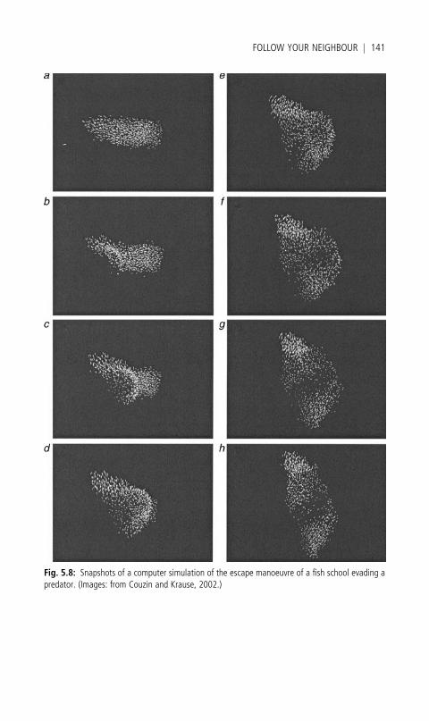
Fig. 5.8: Snapshots of a computer simulation of the escape manoeuvre of a fish school evading apredator. (Images: from Couzin and Krause, 2002.)
FOLLOW YOUR NEIGHBOUR j 141

body sizes can sort a group of fish into large and small. A naive obser-
ver, seeing this, might think that big fish actively seek out other big fish
and so on—and in fact this is often what biologists have assumed when
they see segregation within populations. But in fact the sorting may
emerge without that kind of complex decision-making at all. All the
same, the outcomemay have evolutionary benefits. Parasites that infect
fishmight spread themselvesmore readily by altering their hosts’ behav-
iour, for example making fish slower or less manoeuvrable so that they
adopt positions more likely to get them eaten. Conversely, a group may
ruthlessly shed individuals that stand out from the rest when predators
are nearby, making the group less likely to draw unwelcome attention—
not because the fish are truly heartless or prejudiced against difference,
butbecause the local behavioural rules they followdiffer for ‘normal’ and
‘odd’ individuals in a way that makes the segregation happen.
Follow the leader
These self-organizing motions seem to deny any need for leaders. But
sometimes a few individuals really do know best—for example, if they
have discovered where food is to be found. When the group’s motion
becomes collective, with each member responding to its neighbours, it
becomes much easier for privileged information of this sort to be
shared among the group for its collective benefit. Couzin and his co-
workers have investigated how this allows moving groups to make
complex decisions in an efficient manner. When they adapted the
model described above so that a certain proportion of individuals all
moved in the same preferred direction, only a small fraction of such
‘informed’ members were needed to guide the whole group in that
direction. And as the group became bigger, this proportion got smaller:
the ‘accuracy’ of the group improved. Real swarms do seem to have this
ability: a swarm of honeybees can find a new nest site with only one in
20 individuals knowing the way to a good location. The key point here is
that these agents who ‘know the right way’do not actually have any way
of letting the others know they have this information—no one in the
group knows who ‘knows best’, or even if there are any informed
individuals at all. But the slight bias on the group motion imposed by
a small number of individuals who all head in the ‘good’ direction is
enough to carry the others along.
142 j NATURE’S PATTERNS: FLOW
What, however, if the group contains a mixture of informed individ-
uals with different, conflicting information? Couzin and colleagues
found that in such cases a consensus always emerges, even if the
different leadership groups are of equal size. With two groups of lead-
ers, each of which has a different preferred direction, the consensus
direction depends on how much these choices differ. The group selects
the average of the two directions, unless these are too diametrically
opposed (more than about 1208 apart), in which case the direction of
the largest leadership group is chosen. In this last case, if the two
groups are of exactly the same size then one or other of the directions
is selected at random.
An averaging consensus might not seem ideal: by selecting the aver-
age of the two ‘leadership’directions, the groupwill be heading towards
neither of the leaders’ goals. But that is not necessarily a problem. If the
two targets are a long way off, averaging takes the group in the right
general direction towards them both, and as it approaches, the angle of
divergence between the two possible routes gets steadily bigger (just as
you can hold two distant objects in your vision at once, but may have to
turn your head from one to the other once you get closer). When this
divergence exceeds the critical angle of 1208, then the group chooses to
head for one target or the other.
In any event, the main conclusion is that the model shows how a
group of interacting individuals can respond to the information gath-
ered by just a few, and can reach a collective decision about how to use
that information even without any sophisticated means of assessing
and discussing it. In this sense, animal groups seem to have a demo-
cratic capacity that we might reasonably deem somewhat enviable.
Crowd psychology
It is one thing to make models of how fish and birds move, for it seems
likely that they are governed primarily by instinct. Using a computer
model of boids or self-propelled particles constrained to follow a few
simple rules in a robotic manner seems to do not too great an injustice
to these creatures’ undoubted complexity. But might people move in
this collective, herd-like fashion, too?
That seems a bold, even an impertinent, thing to suggest. But it is
surely a whole lot less impertinent than the approaches taken in some
FOLLOW YOUR NEIGHBOUR j 143
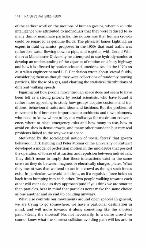
of the earliest work on the motions of human groups, wherein so little
intelligence was attributed to individuals that they were reduced to so
many dumb, inanimate particles: the notion was that human crowds
could be regarded as genuine fluids. The physicist James Lighthill, an
expert in fluid dynamics, proposed in the 1950s that road traffic was
rather like water flowing down a pipe, and together with Gerald Whi-
tham at Manchester University he attempted to use hydrodynamics to
develop an understanding of the vagaries of motion on a busy highway
and how it is affected by bottlenecks and junctions. And in the 1970s an
Australian engineer named L. F. Henderson wrote about ‘crowd fluids’,
considering them as though they were collections of randomly moving
particles, like those of a gas, and charting the statistical distributions of
different walking speeds.
Figuring out how people move through space does not seem to have
been felt as a strong priority by social scientists, who have found it
rather more appealing to study how groups acquire customs and tra-
ditions, behavioural traits and ideas and fashions. But the problem of
movement is of immense importance to architects and town planners,
who need to know where to lay out walkways for maximum conveni-
ence, where to place emergency exits and how many to use, how to
avoid crushes in dense crowds, and many other mundane but very real
problems linked to the way we use space.
Motivated by the sociological notion of ‘social forces’ that govern
behaviour, Dirk Helbing and Peter Molnar of the University of Stuttgart
developed a model of pedestrian motion in the mid-1990s that posited
the operation of forces of attraction and repulsion between individuals.
They didn’t mean to imply that these interactions exist in the same
sense as they do between magnets or electrically charged plates. What
they meant was that we tend to act in a crowd as though such forces
exist. In particular, we avoid collisions, as if a repulsive force holds us
back from bumping into each other. Two people walking towards each
other will veer aside as they approach (and if you think we are smarter
than particles, bear in mind that particles never make the same choice
as one another and so end up colliding anyway).
What else controls our movements around open spaces? In general,
we are trying to go somewhere: we have a particular destination in
mind, and will move towards it along something like the shortest
path. (Really the shortest? No, not necessarily. In a dense crowd we
cannot know what the shortest collision-avoiding path will be; and in
144 j NATURE’S PATTERNS: FLOW

other situations our steps might be diverted by other factors, as we will
see.) We each have our own preferred walking speed, and will speed up
until we attain this, unless something prevents us from doing so.
These were the simple ingredients of Helbing and Molnar’s model.
You can see that it assumes rather uncomplicated, single-minded ped-
estrians. On a crowded day in the shopping precinct, that is perhaps not
a bad description of what we are. What sort of crowd motion, then, do
these rules produce? Helbing has applied the model to a wide range of
situations: negotiating busy intersections, for example, or passing
through unmarked doorways. One of the simplest situations places
the walkers in a corridor, travelling in both directions. (The corridor
could as easily be a pavement.) If the crowd density is high, there is
apparently a recipe here for chaos and congestion. What emerges,
however, is a surprising degree of order (Fig. 5.9a).
The pedestrians arrange themselves into counter-flowing streams,
trailing in each other’s footsteps. This might not seem surprising at all,
for obviously it makes sense to follow the person in front of you: that
way, you are far less likely to collide with someone coming the other
way. But there is no rule to that effect in the model prescription—
nothing to generate ‘following’ behaviour. This simply appears once
the rules are enacted. Of course, it is possible, indeed likely, that we do
show an active tendency to follow one another and form streams—if
such an impulse is included in the pedestrian model, then the bands
form more quickly, and in fact are evident even before two counter-
flowing groupsmeet. But the point is that this ingredient is not essential
for streaming to occur: it emerges from the propensity for collision-
avoidance. There is ample evidence that streaming really does occur,
and you have no doubt seen it for yourself (Fig. 5.9b).
Fig. 5.9: Computer simulations of pedestrians moving in oppositedirections down a corridor show that they organize themselves intocounterflowing streams, even though there is no explicit prescription forthis in the ‘rules’ of the model (a). Such behaviour is commonly seen inreal life (b). (Photo b: Michael Schreckenberg, University of Duisburg.)
FOLLOW YOUR NEIGHBOUR j 145
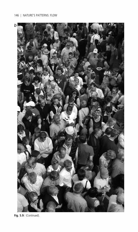
Fig. 5.9: (Continued).
146 j NATURE’S PATTERNS: FLOW

Ant motorways
This sort of ‘lane formation’ among walkers is not unique to humans. It
is strikingly exhibited by army ants (Eciton burchelli), voracious carni-
vores that carry out truly terrifying raids on their arthropod prey. Bands
of several hundred thousand individuals may form trails many metres
wide and over 100 m long leading from their colony to the prey. The
raid has to be finished by dusk, since the ants are inactive at night, and
so they have no time to lose. The trails are divided into lanes that are
used selectively by individuals setting out from the colony or returning
back carrying their prey (Fig. 5.10).
Ants certainly may follow where others have gone before. This is one
of the key aspects of their foraging behaviour: each antmarks its path by
laying down a pheromone, and other ants are drawn towards this
chemical trail. They seek out the highest pheromone concentration,
which tends to keep them travelling along a previously marked path
rather than wandering off on their own. Thus, trails become self-
reinforcing: the more ants that travel that way, the more strongly the
route is chemically marked, and so the more likely others are to use it.
This reinforcement ensures that prey are located efficiently: once a few
successful individuals have found the way there, their pheromone
footsteps will guide others. If, on the other hand, a small group of ants
gets separated from the nest and so loses its return path, it may mill
around aimlessly in a circle, each following the other and not realizing
that the path leads nowhere (Fig. 5.11).
This trail-following behaviour gives rise to characteristic branching
patterns in army-ant raids (Fig. 5.12a), which can be mimicked by
computer models that include the self-amplifying mechanism of
pheromone release (Fig. 5.12b). How, though, do the trails get divided
into lanes designated for advancing and returning workers (Fig. 5.10)?
Iain Couzin and his colleague Nigel Franks at Bristol University think
that the answer lies in the ants’ wish to avoid collisions, particularly
with those coming in the other direction.
Army ants do not have good vision (they are in fact almost blind), but
they can literally feel the presence of others that come into physical
contact. They also have antennae that extend their tactile field in front
of them. Couzin and Franks assumed that if other ants come within this
field, an ant will change direction, veering off its initial course. When
notmanoeuvring out of the paths of others, the ants seek out and follow
a pheromone trail, moving to where the concentration is highest.
FOLLOW YOUR NEIGHBOUR j 147
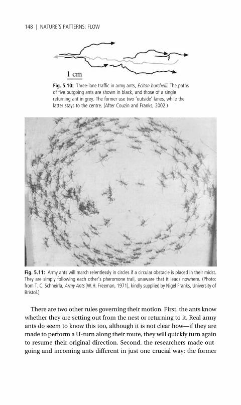
There are two other rules governing their motion. First, the ants know
whether they are setting out from the nest or returning to it. Real army
ants do seem to know this too, although it is not clear how—if they are
made to perform a U-turn along their route, they will quickly turn again
to resume their original direction. Second, the researchers made out-
going and incoming ants different in just one crucial way: the former
Fig. 5.10: Three-lane traffic in army ants, Eciton burchelli. The pathsof five outgoing ants are shown in black, and those of a singlereturning ant in grey. The former use two ‘outside’ lanes, while thelatter stays to the centre. (After Couzin and Franks, 2002.)
Fig. 5.11: Army ants will march relentlessly in circles if a circular obstacle is placed in their midst.They are simply following each other’s pheromone trail, unaware that it leads nowhere. (Photo:from T. C. Schneirla, Army Ants [W.H. Freeman, 1971], kindly supplied by Nigel Franks, University ofBristol.)
148 j NATURE’S PATTERNS: FLOW
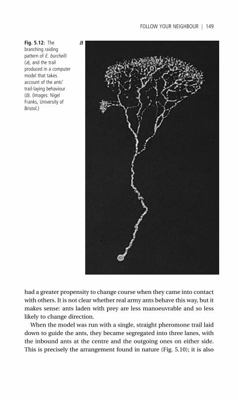
had a greater propensity to change course when they came into contact
with others. It is not clear whether real army ants behave this way, but it
makes sense: ants laden with prey are less manoeuvrable and so less
likely to change direction.
When the model was run with a single, straight pheromone trail laid
down to guide the ants, they became segregated into three lanes, with
the inbound ants at the centre and the outgoing ones on either side.
This is precisely the arrangement found in nature (Fig. 5.10); it is also
Fig. 5.12: Thebranching raidingpattern of E. burchelli(a), and the trailproduced in a computermodel that takesaccount of the ants’trail-laying behaviour(b). (Images: NigelFranks, University ofBristol.)
FOLLOW YOUR NEIGHBOUR j 149
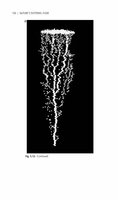
Fig. 5.12: (Continued).
150 j NATURE’S PATTERNS: FLOW
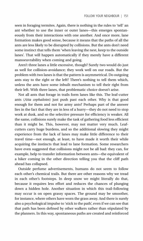
seen in foraging termites. Again, there is nothing in the rules to ‘tell’ an
ant whether to use the inner or outer lanes—this emerges spontan-
eously from their interactions with one another. And once more, lane
formation makes good sense, because it means that the paths of all the
ants are less likely to be disrupted by collisions. But the ants don’t need
some instinct that tells them ‘when leaving the nest, keep to the outside
lanes’. That will happen automatically if they merely have a different
manoeuvrability when coming and going.
Aren’t three lanes a little excessive, though? Surely two would do just
as well for collision-avoidance; they work well on our roads. But the
problemwith two lanes is that the pattern is asymmetrical. Do outgoing
ants stay to the right or the left? There’s nothing to tell them which,
unless the ants have some inbuilt mechanism to tell their right from
their left. With three lanes, that problematic choice doesn’t arise.
Not all ants that forage in trails form lanes like this. The leaf-cutter
ants (Atta cephalotes) just push past each other. Why is that good
enough for them and not for army ants? Perhaps part of the answer
lies in the fact that they are in less of a hurry—they do not need to stop
work at dusk, and so the selective pressure for efficiency is weaker. All
the same, collisions surely make the task of gathering food less efficient
than it might be. This, however, may not matter very much. Leaf-
cutters carry huge burdens, and so the additional slowing they might
experience from the lack of lanes may make little difference to their
travel time—not enough, at least, to have made it worth their while
acquiring the instincts that lead to lane formation. Some researchers
have even suggested that collisions might not be all bad: they can, for
example, help to transfer information between ants—the equivalent of
a hiker coming in the other direction telling you that the cliff path
ahead has collapsed.
Outside perfume advertisements, humans do not seem to follow
each other’s chemical trails. But there are other reasons why we tread
in each other’s footsteps. In deep snow we might literally do that,
because it requires less effort and reduces the chances of plunging
down a hidden hole. Another situation in which this trail-following
may occur is on open grassy spaces. The ground may be smoother,
for instance, where others have worn the grass away. And there is surely
also a psychological impulse to ‘stick to the path’, even if we can see that
that path has been defined by other walkers rather than stipulated by
the planners. In this way, spontaneous paths are created and reinforced
FOLLOW YOUR NEIGHBOUR j 151
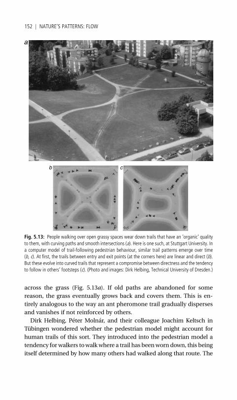
across the grass (Fig. 5.13a). If old paths are abandoned for some
reason, the grass eventually grows back and covers them. This is en-
tirely analogous to the way an ant pheromone trail gradually disperses
and vanishes if not reinforced by others.
Dirk Helbing, Peter Molnar, and their colleague Joachim Keltsch in
Tubingen wondered whether the pedestrian model might account for
human trails of this sort. They introduced into the pedestrian model a
tendency for walkers towalkwhere a trail has beenworndown, this being
itself determined by how many others had walked along that route. The
Fig. 5.13: People walking over open grassy spaces wear down trails that have an ‘organic’ qualityto them, with curving paths and smooth intersections (a). Here is one such, at Stuttgart University. Ina computer model of trail-following pedestrian behaviour, similar trail patterns emerge over time(b, c). At first, the trails between entry and exit points (at the corners here) are linear and direct (b).But these evolve into curved trails that represent a compromise between directness and the tendencyto follow in others’ footsteps (c). (Photo and images: Dirk Helbing, Technical University of Dresden.)
152 j NATURE’S PATTERNS: FLOW
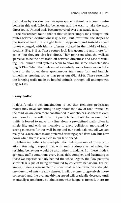
path taken by a walker over an open space is therefore a compromise
between this trail-following behaviour and the wish to take the most
direct route. Unused trails became covered over at a steady rate.
The researchers found that at first walkers simply took straight-line
routes between destinations (Fig. 5.13b). But, over time, the shapes of
the trails altered: the straight lines disappeared, and instead curved
routes emerged, with islands of grass isolated in the middle of inter-
sections (Fig. 5.13c). These routes look less geometric and more ‘or-
ganic’; but they are also less direct. They represent what the walkers
‘perceive’ to be the best trade-off between directness and ease of walk-
ing. Real human trail systems seem to show the same characteristics
(Fig. 5.13a). When the trails are all essentially going from one end of a
space to the other, these spontaneous trails may fork and branch,
sometimes creating routes that peter out (Fig. 5.14). These resemble
the foraging trails made by hoofed animals through tall undergrowth
(Fig. 5.14c).
Heavy traffic
It doesn’t take much imagination to see that Helbing’s pedestrian
model may have something to say about the flow of road traffic. On
the road we are even more constrained in our choices, so there is even
less room for free will to disrupt predictable, robotic behaviour. Road
traffic is forced to move in a line along a pre-defined path, often in
single file, and with an incentive to avoid collisions, motivated by
strong concerns for our well-being and our bank balance. All we can
really do is accelerate to our preferred cruising speed if we can, but slow
down when there is a vehicle in our lane ahead.
Helbing and others have adapted the pedestrian model to this situ-
ation. You might expect that, with such a simple set of rules, the
resulting behaviour would be also rather mundane. But these models
generate traffic conditions every bit as rich, complex, and frustrating as
those we experience daily behind the wheel. Again, the flow patterns
show clear signs of being dominated by collective behaviour. For ex-
ample, it seems reasonable to suspect that, as the traffic on a straight,
one-lane road gets steadily denser, it will become progressively more
congested and the average driving speed will gradually decrease until
eventually a jam forms. But that is not what happens. Instead, there are
FOLLOW YOUR NEIGHBOUR j 153
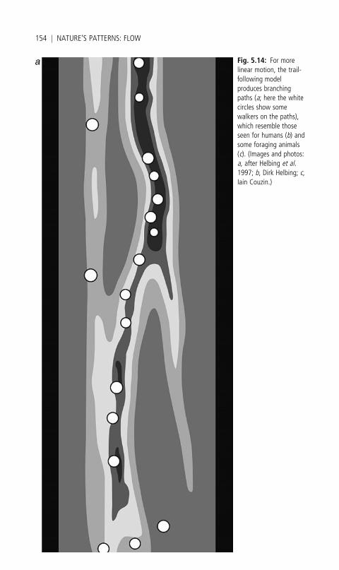
Fig. 5.14: For morelinear motion, the trail-following modelproduces branchingpaths (a; here the whitecircles show somewalkers on the paths),which resemble thoseseen for humans (b) andsome foraging animals(c). (Images and photos:a, after Helbing et al.1997; b, Dirk Helbing; c,Iain Couzin.)
154 j NATURE’S PATTERNS: FLOW

rather abrupt switches between steady flow and almost immobile jams,
once a critical threshold in traffic density (the number of vehicles per
km of road, say) is exceeded. This is again analogous to a phase tran-
sition: a marked shift in ‘global’ behaviour brought about by only a
small change in conditions. It is literally as though the traffic ‘freezes’,
changing from liquid-like flow to solid-like stasis.
This sudden triggering of a jam is seen in a traffic model devised by
Kai Nagel and Michael Schreckenberg, working in Germany in the early
1990s, which has more or less the rules indicated above.* Here a series
of cars drives in procession down a straight road, all of them attaining
Fig. 5.14: (Continued).
*Another ingredient is a small amount of randomness in the speeding up and slowing down
of each vehicle, to account for the fact that no one (whatever they might like to think) drives
perfectly.
FOLLOW YOUR NEIGHBOUR j 155
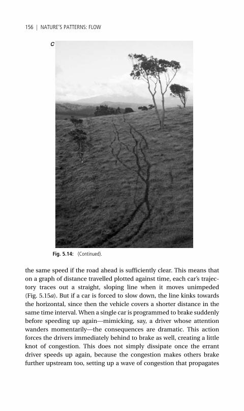
the same speed if the road ahead is sufficiently clear. This means that
on a graph of distance travelled plotted against time, each car’s trajec-
tory traces out a straight, sloping line when it moves unimpeded
(Fig. 5.15a). But if a car is forced to slow down, the line kinks towards
the horizontal, since then the vehicle covers a shorter distance in the
same time interval. When a single car is programmed to brake suddenly
before speeding up again—mimicking, say, a driver whose attention
wanders momentarily—the consequences are dramatic. This action
forces the drivers immediately behind to brake as well, creating a little
knot of congestion. This does not simply dissipate once the errant
driver speeds up again, because the congestion makes others brake
further upstream too, setting up a wave of congestion that propagates
Fig. 5.14: (Continued).
156 j NATURE’S PATTERNS: FLOW
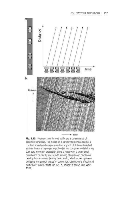
Fig. 5.15: Phantom jams in road traffic are a consequence ofcollective behaviour. The motion of a car moving down a road at aconstant speed can be represented on a graph of distance travelledagainst time as a sloping straight line (a). In a computer model of manysuch cars moving in procession along a motorway, a single smalldisturbance caused by one vehicle slowing abruptly and briefly candevelop into a complex jam (b, dark bands), which moves upstreamand splits into several ‘waves’ of congestion. Observations of real roadtraffic have shown effects like this (c). (Images b and c: from Wolf,1999.)
FOLLOW YOUR NEIGHBOUR j 157
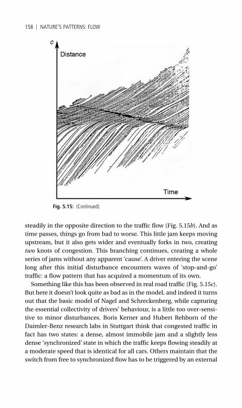
steadily in the opposite direction to the traffic flow (Fig. 5.15b). And as
time passes, things go from bad to worse. This little jam keeps moving
upstream, but it also gets wider and eventually forks in two, creating
two knots of congestion. This branching continues, creating a whole
series of jams without any apparent ‘cause’. A driver entering the scene
long after this initial disturbance encounters waves of ‘stop-and-go’
traffic: a flow pattern that has acquired a momentum of its own.
Something like this has been observed in real road traffic (Fig. 5.15c).
But here it doesn’t look quite as bad as in the model, and indeed it turns
out that the basic model of Nagel and Schreckenberg, while capturing
the essential collectivity of drivers’ behaviour, is a little too over-sensi-
tive to minor disturbances. Boris Kerner and Hubert Rehborn of the
Daimler-Benz research labs in Stuttgart think that congested traffic in
fact has two states: a dense, almost immobile jam and a slightly less
dense ‘synchronized’ state in which the traffic keeps flowing steadily at
a moderate speed that is identical for all cars. Others maintain that the
switch from free to synchronized flow has to be triggered by an external
Fig. 5.15: (Continued).
158 j NATURE’S PATTERNS: FLOW
disturbance, such as a bottleneck on the road or a junction where
another traffic stream joins.
Such disturbances are of course common on real roads, and may be
responsible for much of the variation and complexity of real traffic.
Dirk Helbing and his colleagues found that an entry junction onto a
motorway, for example, can induce all kinds of traffic jams, from knots
that move upstream or stay pinned to a point on the road, to oscillatory
waves of congestion or solid block-like jams.
These models show that traffic flow has its own characteristic and
robust patterns in time and space that emerge spontaneously and
suddenly from the interaction of many individuals. This can make
jams seem like a rather fundamental and inevitable part of life on the
road; but the message need not be so gloomy. By helping us to under-
stand under what conditions congestion and jams form, traffic models
may enable us to lessen the chances of their happening, for example by
appropriate design of road layouts, of speed restrictions, or of lane-
changing rules. This might not only make the roads more pleasant, but
could also make them safer, while reducing pollution. And models that
can predict traffic flow on a real road network, based on measurements
of traffic at a few key locations, could be valuable for planning a route
or for alerting road authorities to potential congestion problems before
they arise. Schemes like this, using models such as those I have de-
scribed, are already being implemented in European and American
cities and urban areas to allow real-time prediction of road use.
Don’t panic
The simulated crowds studied by Helbing and his colleagues are gen-
erally rather well-behaved, finding collective modes of movement that
ease the flow and enable people to move past each other with the
minimum of jostling and discomfort. When two such crowds converge
at a doorway and try to pass through from opposite directions, they
even display what looks like good manners, standing back from time to
time for walkers coming the other way. (Of course, these ‘manners’ are
illusory, since the simulated walkers have no scruples; their apparent
thoughtfulness is prompted merely by the rule that avoids collisions.)
But not all crowds are so civilized. In crowd disasters, panic can lead
people to push others over and trample them. Riots, building fires, and
FOLLOW YOUR NEIGHBOUR j 159
crushes at sports stadiums, rock concerts, and other public gatherings
have in the past claimed many lives as a result of the uncontrolled
movements of crowds that, in their terror or excitement, have ceased to
show anything like the ‘wisdom’ with which they are fashionably at-
tributed.
In 1999 Helbing teamed up with Tamas Vicsek and his colleague Illes
Farkas in Budapest to try to understand what happens when a crowd
panics. They studied how the ‘model pedestrians’move when they want
to get somewhere so quickly that the desire for speed overwhelms the
impulse not to come into contact. The researchers found that a crowd
like this can become jammed if all the individuals try to pass through a
single doorway in a simulation of ‘escape panic’. As walkers press in
against one another in the dense throng in front of the door, they can
become locked into arch-shaped lines, unable to move forward. It is
precisely this sort of jamming that gives masonry arches their stability:
the stones push against their neighbours to form a robust structure,
held together by friction, which resists the tug of gravity. Such arches
are also known to appear in grainy materials as they drop through a
hole, which is why salt can get stuck in the salt cellar even though each
of the individual grains is small enough to pass through the hole. Here,
then, the ‘crowd fluid’ starts to act more like a ‘crowd powder’. The
result is counterintuitive in a rather chilling way: as everyone tries to
move faster, the crowd actually exits through a doorway more slowly
than it would if the individuals kept to a more moderate pace. The
pressures that build up in the jammed crowd can be frightening: in real
crowd disasters they have been large enough to bend steel bars and
knock over walls.
Real animals do seem to behave this way. It is not the kind of
experiment one can conduct ethically with human subjects, of course,
and one winces even to think of it being done with mice. But Caesar
Saloma and colleagues at the University of the Philippines, who did this
in 2003, apparently caused no lasting harm to their subjects, which had
to escape from a chamber that was being slowly flooded. They found
that the mice showed just the kind of ‘escape panic’ exhibited by the
computer model, and that the flow through the exit had the predicted
feature of occurring in bursts of different sizes—very much like, in fact,
the self-organized avalanches of the sand-pile model I described in the
previous chapter.
160 j NATURE’S PATTERNS: FLOW

Because of his work on pedestrian motion and particularly on crowd
panic, Dirk Helbing was consulted in 2006 about crowd control for the
annual pilgrimage of Muslims to Mecca in Saudi Arabia. This event,
called the Hajj, draws up to four million pilgrims, and the threat of
crowd disaster has been ever present. Hundreds of lives have been lost
in the past—in 1990 over 1,000 people were killed in a stampede in a
pedestrian tunnel leading out from Mecca to the nearby town of Mina,
where a ritual stoning takes place.
This stoning has been a flashpoint for several crowd disasters. The
pilgrims gather in Mina to cast stones at pillars called the jamarat, re-
enacting the stoning of the devil by Abraham. To ease congestion, the
three pillars have been replaced by elongated, elliptical structures more
like walls, and a two-tiered ‘bridge’ has been built so that more pilgrims
can gain access to the jamarat at the same time. But these measures
have proved inadequate: pilgrims were trampled to death during
the ritual on six occasions since 1994. The disaster in January 2006
was one of the worst: over 300 pilgrims died, and many more were
injured. The Saudi authorities organizing the Hajj realized that some-
thing had to be done. Could Helbing’s crowd model help?
For the 2006 event, the authorities had installed video cameras to
monitor the movements of the crowd. They allowed Helbing and his
colleagues to study the footage, hoping that this might reveal how the
crush became fatal. What the researchers saw surprised and shocked
them.
As the crowds on the Jamarat Bridge became denser, the steady flow
changed to stop-and-go waves like those in heavy traffic (Fig. 5.16a)—
something that had not been so clearly seen before in crowd motion.
But then, as the throng thickened still further, this motion, which was
uncomfortable and frustrating but nonetheless relatively orderly, gave
way to another kind. People became clustered into knots, reminiscent
of the eddies of fluid flow, which swirled around in all directions
(Fig. 5.16b). Pilgrims were pushed here and there, powerless to do
anything about it, with enough force to knock people off their feet. If
they stumbled, they might have no chance to get up again, nor could
their neighbours avoid trampling on them. The movement looked
startlingly like turbulence in a rushing liquid.
This ‘crowd turbulence’ is not predicted by the simple models of
pedestrian motion or crowd panic. Helbing and his colleagues think
that it is triggered when individuals alter their behaviour in response to
FOLLOW YOUR NEIGHBOUR j 161
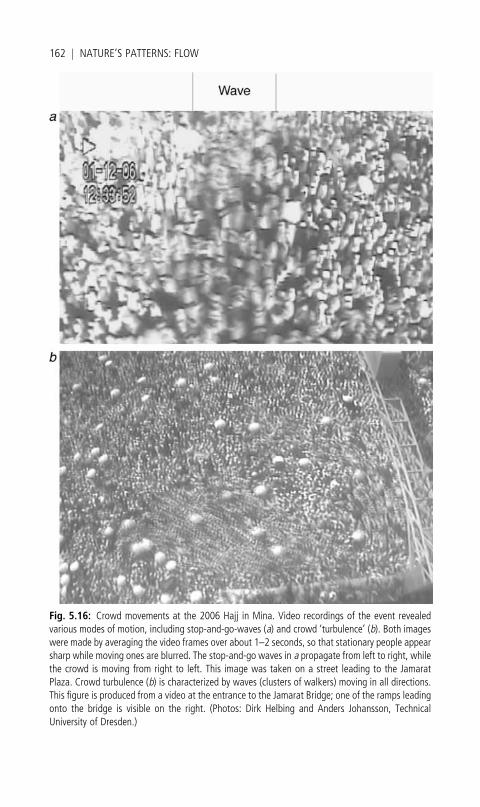
Fig. 5.16: Crowd movements at the 2006 Hajj in Mina. Video recordings of the event revealedvarious modes of motion, including stop-and-go-waves (a) and crowd ‘turbulence’ (b). Both imageswere made by averaging the video frames over about 1–2 seconds, so that stationary people appearsharp while moving ones are blurred. The stop-and-go waves in a propagate from left to right, whilethe crowd is moving from right to left. This image was taken on a street leading to the JamaratPlaza. Crowd turbulence (b) is characterized by waves (clusters of walkers) moving in all directions.This figure is produced from a video at the entrance to the Jamarat Bridge; one of the ramps leadingonto the bridge is visible on the right. (Photos: Dirk Helbing and Anders Johansson, TechnicalUniversity of Dresden.)
162 j NATURE’S PATTERNS: FLOW

the crush: instead of being passively pushed along by the crowd, people
try to ease the squeezing they experience by pushing back. The ‘crowd
fluid’ becomes animated, spontaneously injecting more energy into the
motion. That is something a simple fluid cannot do, and so it is no
surprise that ‘crowd turbulence’ doesn’t exactly mirror ordinary
turbulence. It does mean, however, that the situation suddenly be-
comes much more violent and dangerous.
The researchers deduced that the onset of this hazardous ‘turbu-
lence’ has a special signature that can be spotted in video recordings.
It happens at a threshold determined not by crowd density alone but
also by how much variation there is in the speed of individuals’ mo-
tions. Together, these two factors define a critical ‘crowd pressure’ at
which turbulence sets in. So real-time monitoring and analysis of video
data on dense crowds can give advance warning of when this highly
dangerous state is about to develop, potentially allowing stewards to
introduce crowd-control measures (such as opening up new exits or
stopping further influx) that might relieve the pressure and avoid a fatal
incident.
That, however, happily did not become necessary in the 2007 Hajj. As
a result of the studies by Helbing’s team, a new route between the
pilgrim camp and the jamarah at Mina was devised, with specific
streets designated for one-way flows and stringent schedules arranged
to limit and distribute the flow of pilgrims. Despite the fact that even
more pilgrims came to the Hajj than were expected, the plan proved a
complete success, and the rituals passed without incident. There could
hardly be a better testament to the value of understanding the patterns
of the crowd.
FOLLOW YOUR NEIGHBOUR j 163
6Into the MaelstromThe Trouble with Turbulence
WHAT would you ask God? The German physicist Werner Hei-
senberg allegedly had this in mind: ‘When I meet God, I am
going to ask him two questions: why relativity? And why
turbulence? I really believe he will have an answer for the first.’
The quote is apparently apocryphal, although not implausible: tur-
bulence was the topic of Heisenberg’s doctoral thesis in 1923. But, like
most such stories, it was coined to make a point: understanding turbu-
lent fluid flow is so hard that neither Heisenberg nor, perhaps, God
could achieve it. Heisenberg’s name might have become linked to the
tale simply because he was better known than Sir Horace Lamb, a
British mathematician and an expert on fluid mechanics, who does
seem to have said something similar in 1932 in an address to the British
Association for the Advancement of Science.*
Whether it is genuine or not, Heisenberg’s remark is illuminating,
because it illustrates different ways in which a scientific problem can be
perplexing. One is that the phenomena themselves lie outside our
mundane experience. The theory of relativity developed by Albert Ein-
stein might, at least from the perspective of the 1930s, be deemed a
piece of deistic obfuscation because it is well hidden in our everyday
world and therefore seems rather superfluous. It is not immediately
clear why any deity would feel the need to build a universe governed by
anything other than the old Newtonian laws of mechanics. Why dictate
that these must give way to strange relativistic effects such as the
shrinking of space and the stretching of time when objects move very
fast? The maths needed to comprehend relativity is hard, but not
*Lamb’s comment was reportedly ‘I am an old man now, and when I die and go to
heaven there are two matters on which I hope for enlightenment. One is quantum electro-
dynamics, and the other is the turbulent motion of fluids. And about the former I am rather
optimistic.’

burdensomely so by the standards of theoretical physics. Yet the con-
cepts involved defy our experience and intuitions.*
Other problems in science may be difficult because they really do
demand a degree of mathematical abstraction and sophistication that
is not accessible to most of us. Superstring theory is somewhat like this:
most of us can see that a lifetime would not be enough to decode its
equations.
But turbulence is difficult and perplexing in yet another way. The
basic question is simple: how do we describe a fast-flowing fluid in
mathematical terms? When flow is vigorous enough, the regular struc-
tures and patterns that we have seen in earlier chapters tend to dissolve,
leaving an apparent chaos that changes with every passing moment
(Fig. 6.1). And yet this does not destroy all structure, for then the liquid
would be pervaded by random motion throughout, so that on average
the flow is merely uniform. We do see patterns in turbulent flow, as Jean
Fig. 6.1: In turbulent flow, the motion of the fluid is chaotic, and yet some coherent structures suchas vortices survive. (Photo: Katepalli Sreenivasan, Yale University.)
*I do not mean to imply that a Newtonian universe would ‘work’; we simply don’t know if it
would or not. Of course, in reality relativity does not supplant Newton’s laws but explains
them as a special case that applies at slow speeds and in moderate gravity. But Heisenberg
was understandably puzzled about why there should be any such distinctions. Many
physicists hope that one day a unified theory will show why relativity is an essential aspect
of the way things are.
INTO THE MAELSTROM j 165
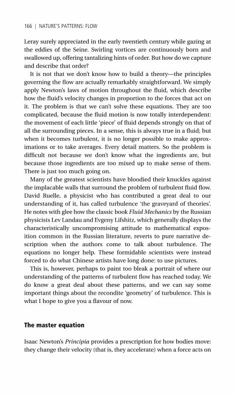
Leray surely appreciated in the early twentieth century while gazing at
the eddies of the Seine. Swirling vortices are continuously born and
swallowed up, offering tantalizing hints of order. But how dowe capture
and describe that order?
It is not that we don’t know how to build a theory—the principles
governing the flow are actually remarkably straightforward. We simply
apply Newton’s laws of motion throughout the fluid, which describe
how the fluid’s velocity changes in proportion to the forces that act on
it. The problem is that we can’t solve these equations. They are too
complicated, because the fluid motion is now totally interdependent:
the movement of each little ‘piece’ of fluid depends strongly on that of
all the surrounding pieces. In a sense, this is always true in a fluid; but
when it becomes turbulent, it is no longer possible to make approx-
imations or to take averages. Every detail matters. So the problem is
difficult not because we don’t know what the ingredients are, but
because those ingredients are too mixed up to make sense of them.
There is just too much going on.
Many of the greatest scientists have bloodied their knuckles against
the implacable walls that surround the problem of turbulent fluid flow.
David Ruelle, a physicist who has contributed a great deal to our
understanding of it, has called turbulence ‘the graveyard of theories’.
He notes with glee how the classic book Fluid Mechanics by the Russian
physicists Lev Landau and Evgeny Lifshitz, which generally displays the
characteristically uncompromising attitude to mathematical expos-
ition common in the Russian literature, reverts to pure narrative de-
scription when the authors come to talk about turbulence. The
equations no longer help. These formidable scientists were instead
forced to do what Chinese artists have long done: to use pictures.
This is, however, perhaps to paint too bleak a portrait of where our
understanding of the patterns of turbulent flow has reached today. We
do know a great deal about these patterns, and we can say some
important things about the recondite ‘geometry’ of turbulence. This is
what I hope to give you a flavour of now.
The master equation
Isaac Newton’s Principia provides a prescription for how bodies move:
they change their velocity (that is, they accelerate) when a force acts on
166 j NATURE’S PATTERNS: FLOW
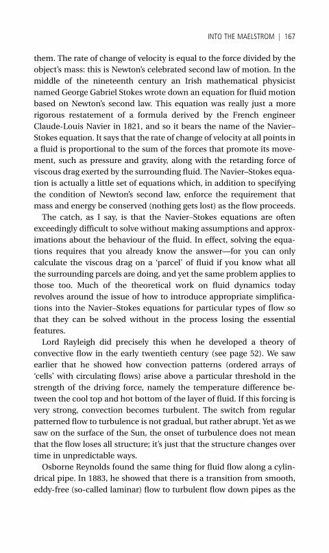
them. The rate of change of velocity is equal to the force divided by the
object’s mass: this is Newton’s celebrated second law of motion. In the
middle of the nineteenth century an Irish mathematical physicist
named George Gabriel Stokes wrote down an equation for fluid motion
based on Newton’s second law. This equation was really just a more
rigorous restatement of a formula derived by the French engineer
Claude-Louis Navier in 1821, and so it bears the name of the Navier–
Stokes equation. It says that the rate of change of velocity at all points in
a fluid is proportional to the sum of the forces that promote its move-
ment, such as pressure and gravity, along with the retarding force of
viscous drag exerted by the surrounding fluid. The Navier–Stokes equa-
tion is actually a little set of equations which, in addition to specifying
the condition of Newton’s second law, enforce the requirement that
mass and energy be conserved (nothing gets lost) as the flow proceeds.
The catch, as I say, is that the Navier–Stokes equations are often
exceedingly difficult to solve without making assumptions and approx-
imations about the behaviour of the fluid. In effect, solving the equa-
tions requires that you already know the answer—for you can only
calculate the viscous drag on a ‘parcel’ of fluid if you know what all
the surrounding parcels are doing, and yet the same problem applies to
those too. Much of the theoretical work on fluid dynamics today
revolves around the issue of how to introduce appropriate simplifica-
tions into the Navier–Stokes equations for particular types of flow so
that they can be solved without in the process losing the essential
features.
Lord Rayleigh did precisely this when he developed a theory of
convective flow in the early twentieth century (see page 52). We saw
earlier that he showed how convection patterns (ordered arrays of
‘cells’ with circulating flows) arise above a particular threshold in the
strength of the driving force, namely the temperature difference be-
tween the cool top and hot bottom of the layer of fluid. If this forcing is
very strong, convection becomes turbulent. The switch from regular
patterned flow to turbulence is not gradual, but rather abrupt. Yet as we
saw on the surface of the Sun, the onset of turbulence does not mean
that the flow loses all structure; it’s just that the structure changes over
time in unpredictable ways.
Osborne Reynolds found the same thing for fluid flow along a cylin-
drical pipe. In 1883, he showed that there is a transition from smooth,
eddy-free (so-called laminar) flow to turbulent flow down pipes as the
INTO THE MAELSTROM j 167
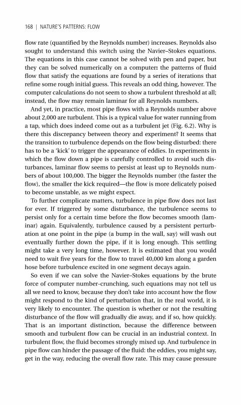
flow rate (quantified by the Reynolds number) increases. Reynolds also
sought to understand this switch using the Navier–Stokes equations.
The equations in this case cannot be solved with pen and paper, but
they can be solved numerically on a computer: the patterns of fluid
flow that satisfy the equations are found by a series of iterations that
refine some rough initial guess. This reveals an odd thing, however. The
computer calculations do not seem to show a turbulent threshold at all;
instead, the flow may remain laminar for all Reynolds numbers.
And yet, in practice, most pipe flows with a Reynolds number above
about 2,000 are turbulent. This is a typical value for water running from
a tap, which does indeed come out as a turbulent jet (Fig. 6.2). Why is
there this discrepancy between theory and experiment? It seems that
the transition to turbulence depends on the flow being disturbed: there
has to be a ‘kick’ to trigger the appearance of eddies. In experiments in
which the flow down a pipe is carefully controlled to avoid such dis-
turbances, laminar flow seems to persist at least up to Reynolds num-
bers of about 100,000. The bigger the Reynolds number (the faster the
flow), the smaller the kick required—the flow is more delicately poised
to become unstable, as we might expect.
To further complicate matters, turbulence in pipe flow does not last
for ever. If triggered by some disturbance, the turbulence seems to
persist only for a certain time before the flow becomes smooth (lam-
inar) again. Equivalently, turbulence caused by a persistent perturb-
ation at one point in the pipe (a bump in the wall, say) will wash out
eventually further down the pipe, if it is long enough. This settling
might take a very long time, however. It is estimated that you would
need to wait five years for the flow to travel 40,000 km along a garden
hose before turbulence excited in one segment decays again.
So even if we can solve the Navier–Stokes equations by the brute
force of computer number-crunching, such equations may not tell us
all we need to know, because they don’t take into account how the flow
might respond to the kind of perturbation that, in the real world, it is
very likely to encounter. The question is whether or not the resulting
disturbance of the flow will gradually die away, and if so, how quickly.
That is an important distinction, because the difference between
smooth and turbulent flow can be crucial in an industrial context. In
turbulent flow, the fluid becomes strongly mixed up. And turbulence in
pipe flow can hinder the passage of the fluid: the eddies, you might say,
get in the way, reducing the overall flow rate. This may cause pressure
168 j NATURE’S PATTERNS: FLOW
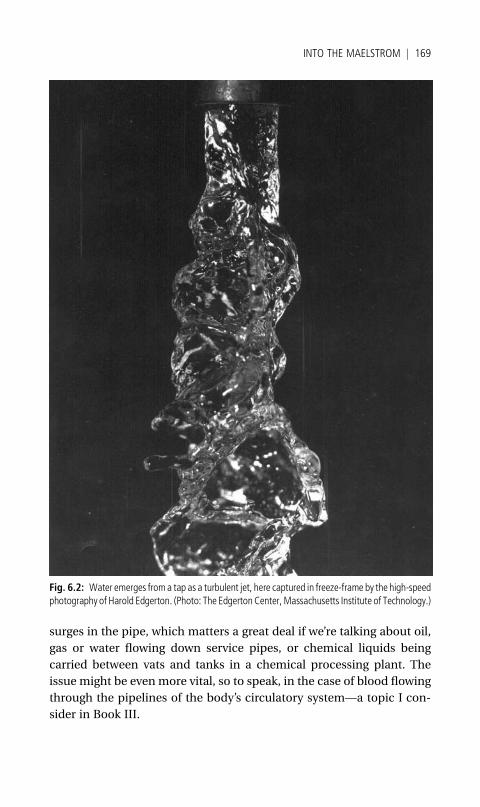
surges in the pipe, which matters a great deal if we’re talking about oil,
gas or water flowing down service pipes, or chemical liquids being
carried between vats and tanks in a chemical processing plant. The
issue might be even more vital, so to speak, in the case of blood flowing
through the pipelines of the body’s circulatory system—a topic I con-
sider in Book III.
Fig. 6.2: Water emerges froma tap as a turbulent jet, here captured in freeze-frame by the high-speedphotography of Harold Edgerton. (Photo: The EdgertonCenter, Massachusetts Institute of Technology.)
INTO THE MAELSTROM j 169
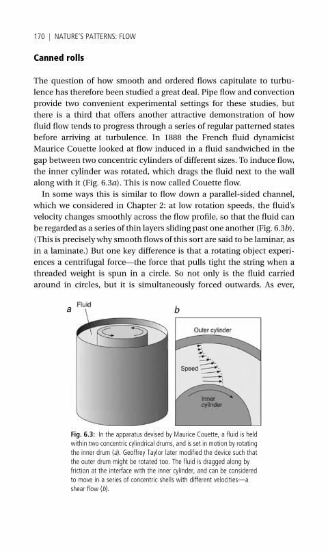
Canned rolls
The question of how smooth and ordered flows capitulate to turbu-
lence has therefore been studied a great deal. Pipe flow and convection
provide two convenient experimental settings for these studies, but
there is a third that offers another attractive demonstration of how
fluid flow tends to progress through a series of regular patterned states
before arriving at turbulence. In 1888 the French fluid dynamicist
Maurice Couette looked at flow induced in a fluid sandwiched in the
gap between two concentric cylinders of different sizes. To induce flow,
the inner cylinder was rotated, which drags the fluid next to the wall
along with it (Fig. 6.3a). This is now called Couette flow.
In some ways this is similar to flow down a parallel-sided channel,
which we considered in Chapter 2: at low rotation speeds, the fluid’s
velocity changes smoothly across the flow profile, so that the fluid can
be regarded as a series of thin layers sliding past one another (Fig. 6.3b).
(This is precisely why smooth flows of this sort are said to be laminar, as
in a laminate.) But one key difference is that a rotating object experi-
ences a centrifugal force—the force that pulls tight the string when a
threaded weight is spun in a circle. So not only is the fluid carried
around in circles, but it is simultaneously forced outwards. As ever,
Fig. 6.3: In the apparatus devised by Maurice Couette, a fluid is heldwithin two concentric cylindrical drums, and is set in motion by rotatingthe inner drum (a). Geoffrey Taylor later modified the device such thatthe outer drum might be rotated too. The fluid is dragged along byfriction at the interface with the inner cylinder, and can be consideredto move in a series of concentric shells with different velocities—ashear flow (b).
170 j NATURE’S PATTERNS: FLOW
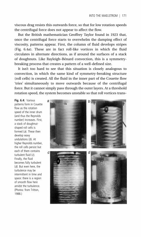
viscous drag resists this outwards force, so that for low rotation speeds
the centrifugal force does not appear to affect the flow.
But the British mathematician Geoffrey Taylor found in 1923 that,
once the centrifugal force starts to overwhelm the damping effect of
viscosity, patterns appear. First, the column of fluid develops stripes
(Fig. 6.4a). These are in fact roll-like vortices in which the fluid
circulates in alternate directions, as if around the surfaces of a stack
of doughnuts. Like Rayleigh–Benard convection, this is a symmetry-
breaking process that creates a pattern of a well-defined size.
It isn’t too hard to see that this situation is closely analogous to
convection, in which the same kind of symmetry-breaking structure
(roll cells) is created. All the fluid in the inner part of the Couette flow
‘tries’ simultaneously to move outwards because of the centrifugal
force. But it cannot simply pass through the outer layers. At a threshold
rotation speed, the system becomes unstable so that roll vortices trans-
Fig. 6.4: Variouspatterns form in Couetteflow as the rotationspeed of the inner drum(and thus the Reynoldsnumber) increases. First,a stack of doughnut-shaped roll cells isformed (a). These thendevelop wavyundulations (b). Athigher Reynolds number,the roll cells persist buteach of them containsturbulent fluid (c).Finally, the fluidbecomes fully turbulent(d). But even here, theturbulence may beintermittent in time andspace: there is a regionof smooth flow hereamidst the turbulence.(Photos: from Tritton,1988.)
INTO THE MAELSTROM j 171

port part of the inner fluid to the outer edge while a return flow
replenishes the inner layer. Not only is the instability of the same
basic nature as that in convection, but the shape of the rolls is the
same: roughly square, as wide as the gap between the inner and outer
cylinders.
The ‘dimensionless number’ that characterizes the driving force for
flow is again the Reynolds number. Here it is defined according to the
velocity of the flow at the surface of the inner cylinder, while the
characteristic dimension of the system is the width of the gap between
the two cylinders. Taylor performed a calculation analogous to
Rayleigh’s for convection, to work out when the roll cells—now known
as Taylor vortices—will appear as the Reynolds number is increased.
Increasing this driving force further by spinning the apparatus more
rapidly produces a progressive elaboration of the basic stripy pattern.
First the roll cells become wavy, undulating up and down around the
cylinders (Fig. 6.4b); then the waves get more complex before becoming
more or less turbulent—after which the stacked stripes reappear with
turbulence inside them (Fig. 6.4c). Finally, when the Reynolds number
is about 1,000 times the value at which the pattern first appears, the
whole column of fluid becomes an unstructured wall of turbulence
(Fig. 6.4d).
But there is more. Taylor realized that the game changes if, instead of
keeping the outer cylinder fixed, we let that rotate as well. Then the
fluid can experience significant centrifugal forces even when the rela-
tive rotation speed of the inner layer with respect to the outer is small,
and so a different balance of forces can be established. Experiments on
a system like this have revealed a menagerie of patterns, too numerous
to show here: interpenetrating spirals, wavy vortices, corkscrew wave-
lets, spiral turbulence. As we have seen, some of these flow patterns
may be analogous to those found in a rotating planetary atmosphere.
Hidden order
If you drive a fluid flow hard enough you will always end up with
turbulence—with chaotic flows that constantly shift. But there are
several ways in which the transition to turbulence may come about.
For convection, the switch tends to be abrupt. In the wakes of shear
flows, such as fluid flowing around an obstacle, turbulence first comes
172 j NATURE’S PATTERNS: FLOW

and goes intermittently, and only takes hold fully when the flow is
faster. In Taylor–Couette flow, turbulence and regular patterns can
coexist for a while in the form of turbulent Taylor vortices. There are
many routes to turbulence, and those taken by particular types of flow
are still being debated.
When turbulence does finally arrive in earnest, however, we might be
tempted to give up looking for any pattern in it all. The trajectories of
the fluid particles become extremely convoluted and ephemeral, and
the Navier–Stokes equations can be solved only by laborious computer
calculations, not by mathematical ingenuity. A turbulent fluid is in a
state of continual instability: you could say that every single thing that
happens in the flow is catastrophic, perturbing everything else. This
means that we generally cannot predict anything about how the flow
will evolve or where any particles carried within it will be at any point in
time. (It does not mean, however, that the Navier–Stokes equations
break down, but instead that these equations no longer have solutions
that remain unchanging in time.)
In this situation, rather than trying to look at the detailed pattern of
flow in terms of streamlines, we are better off just asking about average
features—in other words, we must forget about individual trajectories
of fluid particles and consider instead their statistical properties. Then,
even apparently random, structureless systems like turbulent fluids
prove to have characteristic forms, just as we found a kind of non-
random ‘order’ emerging from the self-organized landslides of sand
grains in Chapter 4. In this way we might be able to distinguish one
kind of apparently chaotic process from another by comparing their
statistical forms. Wewill see in Book III some further illustrations of this
important concept of ‘statistical form’.
The idea that turbulent flows have a generic statistical ‘shape’ which
can be measured quantitatively has been explored throughout the last
century. In the 1920s the Englishman Lewis Fry Richardson proposed
that the ‘universal’ properties of turbulence should become apparent if
we divide it up into the average ‘global’ fluid velocity and the deviations
from that average (the fluctuations) at each point. We can think of a
fluid as having a particular flow velocity (speed and direction) at every
point (a ‘velocity field’), as though each little parcel of fluid were like
one of the swarming particles we encountered in the previous chapter.
Most turbulent flows have non-zero mean velocities: the fluid does ‘get
somewhere’, albeit in a haphazard fashion. Think, for example, of the
INTO THE MAELSTROM j 173
turbulent wake in river flow past a pillar, or a turbulent jet of smoke
exhaled by an office worker as he stands fashionably exiled in the cold
outdoors. Richardson suggested that the generic behaviour of turbu-
lence resides in the statistics of the fluctuations, from which any aver-
age flow must first be subtracted.
He proposed that any structure buried in the fluctuating, chaotic part
of the velocity field could be revealed by considering how the differ-
ences in velocity at two points within the flow vary as the points get
farther apart. There is no single answer to this: it’s a matter of collecting
statistics. If the flow is totally random at all scales, the velocity at one
point will bear no relation to that at any other: all differences in velocity
will occur with equal probability as the points get further apart. If the
flow has a structure, however, like a convection cell, the velocities at
different points will tend to be related to one another in some non-
random way, so that knowing one allows us to predict (or at least
estimate) the other. In such a case, the velocities are said to be correl-
ated. For example, the velocities in adjacent edges of two roll cells are
not independent: if the fluid at a point on one edge is going upwards,
we can be sure that the fluid at a corresponding point on the edge of the
other cell is also moving upwards at about the same speed, because
adjacent rolls are always counter-rotating.
In economics, some market traders spend a lot of time looking for
correlations between stock prices, so that one may be forecast from
another, or so that the price at some point in the future can be deduced
from that today. It seems clear that correlations in time disappear
rather quickly in stock price fluctuations—but if they can be glimpsed,
there may be money to be made if you are swift enough. As it happens,
it has been suggested (albeit controversially) that price correlations in
economics may show some similarity to those of turbulent fluid flow—
in which case, talk of ‘market turbulence’ is not purely metaphorical.
If turbulence has inherent structures that distinguish it from utter
randomness, there will be some correlation between the velocities at
different points in the flow. Intuitively we should expect that in a
chaotic flow such correlations, if they exist at all, will be less strong
the further apart the points are. Notice that in a perfectly ordered array
of Rayleigh–Benard convection cells this is not the case: the correl-
ations are very long-ranged, since the cells are arranged in an orderly
manner. Yet experiments have shown not only that there are correl-
ations in turbulence, but that these have a remarkably long reach,
174 j NATURE’S PATTERNS: FLOW
generally extending over almost the entire width of the flow. It is as
though individuals in a jabbering crowd were able to converse with one
another from opposite sides of a room.
These correlations make a description of turbulence a subtle busi-
ness. They are responsible for its elegant, baroque beauty, a confection
of swirling, vortex-like structures of many different sizes. Fully fledged
turbulence is often patchy, in fact resembling a sluggish river, in which
regions of intense disorder and ‘swirliness’ are superimposed on amore
quiescent background. We saw in Chapter 2 that one of the fundamen-
tal structures of turbulence is the whirlpool-like vortex or eddy. But
whereas in pre-turbulent flow the eddies may form highly regular
patterns such as Karman vortex streets, turbulent eddies are formed
over a very wide range of size scales, and they are transient (like
Jupiter’s Great Red Spot) and might appear anywhere in the flow.
Eddies carry much of the energy of a turbulent flow. Whereas in a
laminar flow the energy is borne along in the direction of the fluid
motion, in turbulent flow only a part of the motional (kinetic) energy
of the fluid gets anywhere—the rest is captured by eddies, which fritter
it away, in the end dissipating it in frictional heating as one parcel of
fluid rubs against another. (This friction is the origin of viscosity.) The
dissipation of kinetic energy happens at very small length scales, as
the molecules in the fluid collide and increase their thermal jiggling. So
the energy that is fed into the flow at large scales, creating big eddies
that we can see, finds its way by degrees down to these small scales
before being dissipated. In other words, there is an energy cascade: big
eddies transfer their energy to smaller eddies, which do likewise at ever
smaller scales. Richardson appreciated this, and in 1922 he coined a
rhyme, inspired by Jonathon Swift’s doggerel about fleas, to describe
the process:
Big whirls have little whirls
that feed on their velocity,
and little whirls have lesser whirls
and so on to viscosity.
In the 1940s the Russian physicist Andrei Kolmogorov put this energy
cascade into precise mathematical form. He proposed that the energy
contained in a turbulent fluid at a length scale d varies in proportion to
the 5/3rd power of d—in other words, it increases as d gets larger at a
rate proportional to slightly less than the square of d. Compare this with
INTO THE MAELSTROM j 175
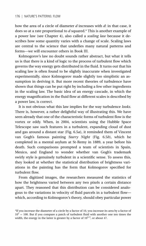
how the area of a circle of diameter d increases with d: in that case, it
does so at a rate proportional to d squared.* This is another example of
a power law (see Chapter 4), also called a scaling law because it de-
scribes how some quantity varies with a change of scale. Scaling laws
are central to the science that underlies many natural patterns and
forms—we will encounter others in Book III.
Kolmogorov’s law no doubt sounds rather abstract, but what it tells
us is that there is a kind of logic to the process of turbulent flow which
governs the way energy gets distributed in the fluid. It turns out that his
scaling law is often found to be slightly inaccurate when investigated
experimentally, since Kolmogorov made slightly too simplistic an as-
sumption in deriving it. But more recent theories of turbulence have
shown that things can be put right by including a few other ingredients
in the scaling law. The basic idea of an energy cascade, in which the
energy magnification in the fluid flow at different scales is described by
a power law, is correct.
It is not obvious what this law implies for the way turbulence looks.
There is, however, a rather delightful way of illustrating this. We have
seen already that one of the characteristic forms of turbulent flow is the
vortex or eddy. When, in 2004, scientists using the Hubble Space
Telescope saw such features in a turbulent, expanding cloud of dust
and gas around a distant star (Fig. 6.5a), it reminded them of Vincent
van Gogh’s famous painting Starry Night (Fig. 6.5b), which he
completed in a mental asylum at St-Remy in 1889, a year before his
death. Such comparisons prompted a team of scientists in Spain,
Mexico, and England to wonder whether van Gogh’s trademark
swirly style is genuinely turbulent in a scientific sense. To assess this,
they looked at whether the statistical distribution of brightness vari-
ations in the painting has the form that Kolmogorov specified for
turbulent flow.
From digitized images, the researchers measured the statistics of
how the brightness varied between any two pixels a certain distance
apart. They reasoned that this distribution can be considered analo-
gous to the variations in velocity of fluid parcels in a turbulent flow—
which, according to Kolmogorov’s theory, should obey particular power
*If you increase the diameter of a circle by a factor of 10, you increase its area by a factor of
102 ¼ 100. But if you compare a patch of turbulent fluid with another one ten times the
width, the energy in the latter is greater by a factor of 105/3, or about 47.
176 j NATURE’S PATTERNS: FLOW

laws.* For Starry Night, these correspondences hold fast with impres-
sive accuracy. In other words, the painting gives a technically accurate
representation of what Kolmogorov’s turbulence ‘looks like’.
The same is true for Van Gogh’s Road with Cypress and Star and
Wheat Field with Crows, both painted in a particularly disturbed period
in early 1890 (the second of these paintings was the last he completed
Fig. 6.5: Turbulence seen in interstellar gas and dust around the star V838 Monocerotis (V838 Mon),about 20,000 light-years away fromEarth in the direction of the constellationMonoceros (a). The imagewas taken by the Hubble Space Telescope in February 2004. The dust is illuminated by a flash of lightemitted fromV383Mon,a red supergiant star, at themiddleof thepicture. This imagemadeastronomersthink of Van Gogh’s famous painting Starry Night (1889) (b). (Photos: a, NASA, the Hubble HeritageTeam (AURA/STScI) and ESA. b, Digital image copyright 2008, Museum ofModern Art/Scala, Florence.)
*To be specific: Kolmogorov’s work led to the prediction that the distribution of velocity
differences between two points, dv, obeys a series of different power laws corresponding to
different powers of dv: there is one law for dv2, one for dv3, and so on. The researchers
searched for similar power-law relationships governing the differences in brightness in Van
Gogh’s painting.
INTO THE MAELSTROM j 177
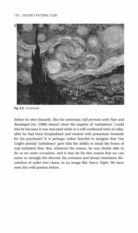
before he shot himself). But his notorious Self-portrait with Pipe and
Bandaged Ear (1888) doesn’t show the imprint of ‘turbulence’. Could
this be because it was executed while in a self-confessed state of calm,
after he had been hospitalized and treated with potassium bromide
for his psychosis? It is perhaps rather fanciful to imagine that Van
Gogh’s mental ‘turbulence’ gave him the ability to intuit the forms of
real turbulent flow. But, whatever the reason, he was clearly able to
do so on some occasions, and it may be for this reason that we can
sense so strongly the discord, the constant and always imminent dis-
solution of order into chaos, in an image like Starry Night. We have
seen this wild pattern before.
Fig. 6.5: (Continued)
178 j NATURE’S PATTERNS: FLOW
Appendix 1
Benard Convection
POLYGONAL convection cells will appear in a thin layer of a viscous
liquid heated gently from below. This is a classic ‘kitchen’
experiment, since it involves little more than heating oil in a
saucepan on a cooker. The base of the pan must be flat and smooth,
however, and preferably also thick to distribute the heat evenly. A skillet
works well. The oil layer need be only about 1–2 mm deep. The flow
pattern can be revealed by sprinkling a powdered spice such as cinna-
mon on to the surface of the oil.
For a more controlled experiment, silicone oil works better. This is
commercially available in a range of viscosities, and a viscosity of
0.5 cm2/s is generally about right. The convection cells can be seen
more clearly if metal powder is suspended in the fluid (see Fig. 3.1).
Bronze powder can be obtained from hardware shops or art material
suppliers. Aluminium flakes can be extracted from the pigment of
‘silver’ model paints by decanting the liquid and then washing the
residual flakes in acetone (nail-varnish remover). These powders will
settle in silicone oil if left to stand.
These procedures are based on:
S. J. VanHook and M. Schatz, ‘Simple demonstrations of pattern for-
mation’, The Physics Teacher 35 (1997): 391.
This paper provides the names and addresses of someUS suppliers of
the substances required.
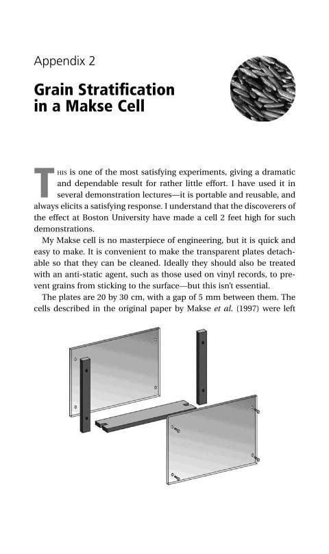
Appendix 2
Grain Stratificationin a Makse Cell
THIS is one of the most satisfying experiments, giving a dramatic
and dependable result for rather little effort. I have used it in
several demonstration lectures—it is portable and reusable, and
always elicits a satisfying response. I understand that the discoverers of
the effect at Boston University have made a cell 2 feet high for such
demonstrations.
My Makse cell is no masterpiece of engineering, but it is quick and
easy to make. It is convenient to make the transparent plates detach-
able so that they can be cleaned. Ideally they should also be treated
with an anti-static agent, such as those used on vinyl records, to pre-
vent grains from sticking to the surface—but this isn’t essential.
The plates are 20 by 30 cm, with a gap of 5 mm between them. The
cells described in the original paper by Makse et al. (1997) were left

open at one end, but an endpiece at both ends ensures that the plates
remain parallel andmeans that the layers can fill up the cell completely,
which gives a more attractive and easily visible effect.
The prettiest results are achieved with coloured sand grains, which
can be bought from some chemical suppliers. But granulated sugar and
ordinary sand (cleaned, from a pet shop or from children’s sand pits)
are easier to get hold of, and have enough of a difference in grain size,
shape and colour to produce visible layering. The sugar grains are larger
and more square—table salt is too similar to sand, and so it doesn’t
segregate well. The best results are obtained by pouring a 50:50 mixture
of grains at a slow and steady rate into one corner of the cell. For a
funnel, all you need is an envelope of about A5 size with the tip of
a corner cut off.
NATURE’S PATTERNS: SHAPES j 181
Bibliography
Anderson, R. S., ‘The attraction of sand dunes’, Nature 379 (1996): 24.
Anderson, R. S., and Bunas, K. L., ‘Grain size segregation and stratigraphy in
Aeolian ripples modeled with a cellular automaton’, Nature 365 (1993): 740.
Aragon, J. L., Naumis, G. G., Bai, M., Torres, M., and Maini, P. K., ‘Kolmogorov
scaling in impassioned van Gogh paintings’, Journal of Mathematical Imaging
and Vision 30 (2008): 275.
Bagnold, R. A., The Physics of Blown Sand and Desert Dunes (London: Methuen,
1941).
Bak, P., How Nature Works (Oxford: Oxford University Press, 1997).
Bak, P., Tang, C., and Wiesenfeld, K., ‘Self-organized criticality. An explanation of
1/f noise’, Physical Review Letters 59 (1987): 381.
Bak, P., and Paczuski, M., ‘Why Nature is complex’, Physics World (December
1993): 39.
Ball, P., Critical Mass (London: Heinemann, 2004).
Barrow, J. D., The Artful Universe (London, Penguin, 1995).
Ben-Jacob, E., Cohen, I., and Levine, H., ‘Cooperative self-organization of micro-
organisms’, Advances in Physics 49 (2000): 395.
Buhl, J., Sumpter, D. J. T., Couzin, I. D., Hale, J. J., Despland, E., Miller, E. R., and
Simpson, S. J., ‘From disorder to order inmarching locusts’, Science 312 (2006):
1402.
Camazine, S., Deneubourg, J.-L., Franks, N. R., Sneyd, J., Theraulaz, G., and
Bonabeau, E., Self-Organization in Biological Systems (Princeton: Princeton
University Press, 2001).
Cannell, D. S., and Meyer, C. W., ‘Introduction to convection’, in Stanley, H. E.,
and Ostrowsky, N. (eds), Random Fluctuations and Patterns Growth (Dor-
drecht: Kluwer, 1988).
Couzin, I. D., and Franks, N. R., ‘Self-organized lane formation and optimized
traffic flow in army ants’, Proceedings of the Royal Society London B 270 (2002):
139.
Couzin, I. D., Krause, J., James, R., Ruxton, G. D., and Franks, N. R., ‘Collective
memory and spatial sorting in animal groups’, Journal of Theoretical Biology
218 (2002): 1.
Couzin, I. D., and Krause, J., ‘Self-organization and collective behavior in verte-
brates’, Advances in the Study of Behavior 32 (2003): 1.
Couzin, I. D., Krause, J., Franks, N. R., and Levin, S. A. ‘Effective leadership and
decision-making in animal groups on the move’, Nature 433 (2005): 513.
Czirok, A., and Vicsek, T., ‘Collective behavior of interacting self-propelled par-
ticles’, Physica A 281 (2000): 17.
Czirok, A., Stanley, H. E., and Vicsek, T., ‘Spontaneously ordered motion of self-
propelled particles’, Journal of Physics A: Mathematical and General 30 (1997):
1375.
Czirok, A., and Vicsek, T., ‘Collective motion’, in Reguera, D., Rubi, M., and Vilar,
J. (eds), Statistical Mechanics of Biocomplexity, Lecture Notes in Physics 527
(Berlin: Springer-Verlag, 1999): 152.
Duran, O., Schwammle, V., and Herrmann, H., ‘Breeding and solitary wave
behavior of dunes’, Physical Review E 72 (2005): 021308.
Endo, N., Taniguchi, K., and Katsuki, A., ‘Observation of the whole process of
interaction between barchans by flume experiment’, Geophysical Research
Letters 31 (2004): L12503.
Forrest, S. B., and Haff, P. K., ‘Mechanics of wind ripple stratigraphy’, Science 255
(1992): 1240.
Frette, V., Christensen, K., Malthe-Sørenssen, A., Feder, J., Jøssang, T., and Mea-
kin, P., ‘Avalanche dynamics in a pile of rice’, Nature 379 (1996): 49.
Glatzmaier, G. A., and Schubert, G., ‘Three-dimensional spherical models of
layered and whole mantle convection’, Journal of Geophysical Research 98
(B12) (1993): 21969.
Gollub, J. P., ‘Spirals and chaos’, Nature 367 (1994): 318.
Grossmann, S., ‘The onset of shear flow turbulence’, Reviews of Modern Physics
72 (2000): 603.
Helbing, D., Keltsch, J., and Molnar, P., ‘Modelling the evolution of human trail
systems’, Nature 388 (1997): 47.
Helbing, D., Farkas, I., and Vicsek, T., ‘Simulating dynamical features of escape
panic’, Nature 407 (2000), 487.
Helbing, D., Molnar, P., Farkas, I. J., and Bolay, K. ‘Self-organizing pedestrian
movement’, Environment and Planning B: Planning and Design 28 (2001): 361.
Helbing, D., ‘Traffic and related self-driven many-particle systems’, Reviews of
Modern Physics 73 (2001): 1067.
Helbing, D., Johansson, A., and Al-Abideen, H. Z., ‘The dynamics of crowd
disasters: an empirical study’, Physical Review E 75 (2007): 046109.
Henderson, L. F., ‘The statistics of crowd fluids’, Nature 229 (1971): 381.
Hersen, P., Douady, S., and Andreotti, B., ‘Relevant length scale of barchan
dunes’, Physical Review Letters 89 (2002): 264301.
Hill, R. J. A., and Eaves, L., ‘Nonaxisymmetric shapes of a magnetically levitated
and spinning water droplet’, Physical Review Letters 101 (2008): 234501.
Hof, B., Westerweel, J., Schneider, T. M., and Eckhardt, B., ‘Finite lifetime of
turbulence in shear flows’, Nature 443 (2006): 59.
Houseman, G., ‘The dependence of convection planform on mode of heating’,
Nature 332 (1988): 346.
Ingham, C. J., and Ben-Jacob, E., ‘Swarming and complex pattern formation in
Paenibacillus vortex studied by imaging and tracking cells’, BMC Microbiology
8 (2008): 36.
Jaeger, H. M., and Nagel, S. R., ‘Physics of the granular state’, Science 255 (1992):
1523.
BIBLIOGRAPHY j 183
Jaeger, H. M., Nagel, S. R., and Behringer, R. P., ‘The physics of granular mater-
ials’, Physics Today (April 1996): 32.
Jullien, R., and Meakin, P., ‘Three-dimensional model for particle-size segrega-
tion by shaking’, Physical Review Letters 69 (1992): 640.
Kemp, M., Visualizations (Oxford: Oxford University Press, 2000).
Kerner, B. S., The Physics of Traffic (Berlin: Springer, 2004).
Kessler, M. A., and Werner, B. T., ‘Self-organization of sorted patterns ground’,
Science 299 (2003): 380.
Knight, J. B., Jaeger, H. M., and Nagel, S. R., ‘Vibration-induced size separation in
granular media: the convection connection’, Physical Review Letters 70 (1993):
3728.
Krantz, W. B., Gleason, K. J., and Caine, N., ‘Patterned ground’, Scientific Ameri-
can 259(6) (1988): 44.
Krause, J., and Ruxton, G. D., Living in Groups (Oxford: Oxford University Press,
2002).
Kroy, K., Sauermann, G., and Herrmann, H. J., ‘Minimal model for sand dunes’,
Physical Review Letters 88 (2002): 054301.
Kroy, K., Sauermann, G., and Herrmann, H. J., ‘Minimal model for aeolian sand
dunes’, Physical Review E 66 (2002): 031302.
Lancaster, N., Geomorphology of Desert Dunes (London: Routledge, 1995).
Landau,L.D., andLifshitz, E.M.,FluidMechanics (Oxford: PergamonPress, 1959).
L’Vov, V., and Procaccia, I., ‘Turbulence: a universal problem’, Physics World 35
(August 1996).
Machetel, P., and Weber, P., ‘Intermittent layered convection in a model mantle
with an endothermic phase change at 670 km’, Nature 350 (1991): 55.
Makse, H. A., Havlin, S., King, P. R., and Stanley, H. E., ‘Spontaneous stratification
in granular mixtures’, Nature 386 (1997): 379.
Manneville, J.-B., and Olson, P., ‘Convection in a rotating fluid sphere and
banded structure of the Jovian atmosphere’, Icarus 122 (1996): 242.
Marcus, P. S., ‘Numerical simulation of Jupiter’s Great Red Spot’, Nature 331
(1988): 693.
Melo, F., Umbanhowar, P. B., and Swinney, H. L., ‘Hexagons, kinks, and disorder
in oscillated granular layers’, Physical Review Letters 75 (1995): 3838.
Metcalfe, G., Shinbrot, T., McCarthy, J. J., and Ottino, J. M., ‘Avalanche mixing of
granular solids’, Nature 374 (1995): 39.
Morris, S. W., Bodenschatz, E., Cannell, D. S., and Ahlers, G., ‘Spiral defect chaos
in large aspect ratio Rayleigh–Benard convection’, Physical Review Letters 71
(1993): 2026.
Mullin, T., ‘Turbulent times for fluids’, in Hall, N. (ed.), Exploring Chaos. A Guide
to the New Science of Disorder (New York: W. W. Norton, 1991).
Nickling, W. G., ‘Aeolian sediment transport and deposition’, in Pye, K. (ed.),
Sediment Transport and Depositional Processes (Oxford: Blackwell Scientific,
1994).
Ottino, J. M., ‘Granular matter as a window into collective systems far from
equilibrium, complexity, and scientific prematurity’, Chemical Engineering
Science 61 (2006): 4165.
Parrish, J. K., and Edelstein-Keshet, L., ‘Complexity, pattern, and evolutionary
trade-offs in animal aggregation’, Science 284 (1999): 99.
184 j BIBLIOGRAPHY
Parteli, E. J. R., and Herrmann, H. J., ‘Saltation transport on Mars’, Physical
Review Letters 98 (2007): 198001.
Perez, G. J., Tapang, G., Lim, M., and Saloma, C., ‘Streaming, disruptive interfer-
ence and power-law behavior in the exit dynamics of confined pedestrians’,
Physica A 312 (2002): 609.
Potts, W. K., ‘The chorus-line hypothesis of manoeuvre coordination in avian
flocks’, Nature 309 (1984): 344.
Rappel, W.-J., Nicol, A., Sarkissian, A., Levine, H., and Loomis,W. F., ‘Self-organized
vortex state in two-dimensionalDictyosteliumdynamics’,Physical ReviewLetters
83 (1999): 1247.
Reynolds, C., ‘Boids’, article available at <http://www.red3d.com/cwr/boids/>.
Reynolds, C. W., ‘Flocks, herds and schools: a distributed behavioral model’,
Computer Graphics 21(4) (1987): 25.
Ruelle, D., Chance and Chaos (London: Penguin, 1993).
Saloma, C., Perez, G. J., Tapang, G., Lim, M., and Palmes-Saloma, C., ‘Self-
organized queuing and scale-free behavior in real escape panic’, Proceedings
of the National Academy of Sciences USA 100 (2003): 11947.Schwammle, V., and Herrmann, H., ‘Solitary wave behaviour of sand dunes’,
Nature 426 (2003): 619.
Scorer, R., and Verkaik, A., Spacious Skies (Newton Abbott: David & Charles,
1989).
Shinbrot, T., ‘Competition between randomizing impacts and inelastic collisions
in granular pattern formation’, Nature 389 (1997): 574.
Sokolov, A., Aranson, I. S., Kessler, J. O., and Goldstein, R. E., ‘Concentration
dependence of the collective dynamics of swimming bacteria’, Physical Review
Letters 98 (2007): 158102.
Sommeria, J., Meyers, S. D., and Swinney, H. L., ‘Laboratory simulation of
Jupiter’s Great Red Spot’, Nature 331 (1988): 689.
Stewart, I., and Golubitsky, M., Fearful Symmetry (London: Penguin, 1993).
Strykowski, P. J., and Sreenivasan, K. R., ‘On the formation and suppression of
vortex ‘‘shedding’’ at low Reynolds numbers’, Journal of Fluid Mechanics 218
(1990): 71.
Sumpter, D. J. T., ‘The principles of collective animal behaviour’, Philosophical
Transactions of the Royal Society B 361 (2005): 5.
Szabo, B., Szollosi, G. J., Gonci, B., Juranyi, Zs., Selmeczi, D., and Vicsek, T. ‘Phase
transition in the collective migration of tissue cells: experiment and model’,
Physical Review E 74 (2006): 061908.
Tackley, P. J., Stevenson, D. J., Glatzmaier, G. A., and Schubert, G., ‘Effects of an
endothermic phase transition at 670 km depth in a spherical model of con-
vection in the Earth’s mantle’, Nature 361 (1993): 699.
Tackley, P. J., ‘Layer cake on plum pudding?’, Nature Geoscience 1 (2008): 157.
Thompson, D’A. W., On Growth and Form (New York: Dover, 1992).
Toner, J., and Tu, Y., ‘Long-range order in a two-dimensional dynamical XY
model: how birds fly together’, Physical Review Letters 75 (1995): 4326.
Tritton, D. J., Physical Fluid Dynamics (Oxford: Oxford University Press, 1988).
Umbanhowar, P. M., Melo, F., and Swinney, H. L., ‘Localized excitations in a
vertically vibrated granular layer’, Nature 382 (1996): 793.
BIBLIOGRAPHY j 185

Umbanhowar, P. M., Melo, F., and Swinney, H. L., ‘Periodic, aperiodic, and
transient patterns in vibrated granular layers’, Physica A 249 (1998): 1.
Van Heijst, G. J. F., and Flor, J. B., ‘Dipole formation and collisions in a stratified
fluid’, Nature 340 (1989): 212.
Vatistas, G. H., ‘A note on liquid vortex sloshing and Kelvin’s equilibria’, Journal of
Fluid Mechanics 217 (1990): 241.
Vatistas, G. H., Wang, J., and Lin, S., ‘Experiments on waves induced in the
hollow core of vortices’, Experiments in Fluids 13 (1992): 377.
Velarde, G., and Normand, C., ‘Convection’, Scientific American 243(1) (1980): 92.
Vicsek, T., Czirok, A., Ben-Jacob, E., Cohen, I., and Shochet, O., ‘Novel type of
phase transition in a system of self-driven particles’, Physical Review Letters 75
(1995): 1226.
Welland, M., Sand: The Never-Ending Story (Berkeley: University of California
Press, 2008).
Werner, B. T., ‘Eolian dunes: computer simulations and attractor interpretation’,
Geology 23 (1995): 1057.
Williams, J. C., and Shields, G., ‘Segregation of granules in vibrated beds’, Powder
Technology 1 (1967): 134.
Wolf, D. E., ‘Cellular automata for traffic simulations’, Physica A 263 (1999): 438.
Worthington, A. M., A Study of Splashes (London: Longmans, Green & Co., 1908).
Zik, O., Levine, D., Lispon, S. G., Shtrikman, S., and Stavans, J., ‘Rotationally
induced segregation of granularmaterials’,Physical ReviewLetters 73 (1994): 644.
186 j BIBLIOGRAPHY

Index
activator-inhibitor systems 84
aeolian deposition 79–83
Alberti, Leon Battista 3
Anderson, Robert 92
angle of repose 95–97
ants 124
swarms and trail patterns 146–151
army ants (Eciton burchelli) 146–151
art, and fluid flow 5–20, 176–178
and science 3–5
Art Nouveau 12–14
artificial life 127, 128
atmospheric circulation 37, 62–65
on other planets 35, 37, 41–45
avalanches 93–110, 180
bacteria, collective motion 129–131
Bacillus subtilis 129, 135, 139
Bagnold, Ralph Alger 77–79, 81, 85, 86, 89
Bak, Per 102, 105, 107, 108
Bandello, Matteo 2
bathtub vortex 35–37, 39
bees, swarming 142
Benard, Henri 31, 50–52
Ben-Jacob, Eshel 129
Bernoulli, Daniel 12, 34
Biesel, Francis 36, 37
birds, flocking, see flocking
boids 126–128
Brazil nut effect 110–113
Buhl, Jerome 133
Bunas, Kirby 92
Busse, Friedrich 55
Cassini, Giovanni Domenico 41
Chang Yen-yuan 16
chemotaxis 131
Chinese art 13, 15, 16
Chladni, Ernst 114
Chladni figures 113–115
Christensen, Kim 109
cloud patterns 31, 33, 51, 62–64
Constable, John 6
convection 50–76, 167, 179
in grains 111–113
Cornish, Vaughan 86
correlations 174–176
Couette flow 170–173
Couette, Maurice 170
Couzin, Iain 136, 137, 139–143, 148
critical states 106, 107
crowd motion 143–146, 159–163
cyclones 37, 38, 49
defects, in convection 58, 59
Derges, Susan 19, 20
Descartes, Rene 12, 121
deserts 77, 79, 84, 86
Dictyostelium discoideum 131, 138, 139
dimensionless numbers 29
droplets, rotating 47, 48
Duchamp, Marcel 6
dunes 77, 78, 83–91
earthquakes 107, 108
Eaves, Laurence 48
eddies 7, 11, 12, 166, 175
see also vortices
Edgerton, Harold 22–25
emergence 127, 128
energy cascade, in turbulence 175, 176
erosion 7
Faraday, Michael 112–114
Farkas, Illes 160
Feder, Jens 109
fingerprints 59
fish, schooling 124, 136–143
flocking 124–143
Flor, Jan-Bert 40
fluid dynamics 26, 165–169
forest fires 107, 108
Forrest, Spencer 82, 83
Franks, Nigel 148
frost heaving 74
galaxies, shapes 45, 47
Gombrich, Ernst 7
granular media 77–123, 180
Great Red Spot, Jupiter 41–45, 175
Gutenberg-Richter law 107
Haeckel, Ernst 4, 12
Haff, Peter 82, 83
Hajj 160–163
Halley, Edmund 64
Haynes, Vance 86
Heisenberg, Werner 164
Helbing, Dirk 144–146, 151–154,
158–163
Helmholtz, Hermann von 35
Herrmann, Hans 88, 90, 91
Hiemenz, Karl 31
Hill, Richard 48
Hong, Daniel 113
Hooke, Robert 41
hydroid 24, 25
hydrological cycle 7
hysteresis 139
hurricanes 49
Japanese art 13, 20
Jugendstil 12
Jullien, Remi 111, 113
Jupiter, atmosphere of 41–45, 175
Katsuki, Atsunari 89, 90
Kelvin, Lord 35, 45
Kelvin-Helmholtz instability 35–37
Kemp, Martin 5
Kerner, Boris 158
Kessler, Mark 74
Karman, Theodore von 31
Karman vortex street 30–33, 175
Keltsch, Joachim 151
keratocytes 135
klinotaxis 131
Kolmogorov, Andrei 175–177
Krantz, William 73, 74
Lamb, Horace 164
laminar flow 28, 29, 167, 170
Landau, Lev 166
landslides, see avalanches
lane formation, in animal motion
145–151
Langton, Chris 127
leaf-cutter ants (Atta cephalotes) 151
Leonardo da Vinci 1–12, 17, 18, 20, 25,
26, 36
Leray, Jean 27, 165
Lifshitz, Evgeny 166
Lighthill, James 144
liquefaction, of grains 78
liquid crystals 59
locusts, banding and swarming 133–135
Machiavelli, Niccolo 7
Maelstrom 39
Makse, Hernan 93–96
Manneville, Jean-Baptiste 42
mantle convection 65–71
Marangoni, Carlo 61
Marangoni convection 60–62
Marcus, Philip 42
Mars, dunes 86, 87, 90, 91
mass extinctions 105, 108
Meakin, Paul 111, 113
Meinhardt, Hans 84
Melo, Francisco 114
Meyers, Steven 43
Molnar, Peter 144, 151
Morland, George 12
Mucha, Alphonse 14
Nagel, Kai 155, 158
Nagel, Sidney 108, 113
Navier, Claude-Louis 167
Navier-Stokes equations 167, 168, 173
188 j INDEX
Newton, Isaac 166, 167
Nordenskjold, Otto 71
ocean circulation 64, 65
Olson, Peter 42
On Growth and Form (Thompson) 24,
25, 67
oscillons 120–122
Ottino, Julio 98
Oyama, Yositisi 98
panic, in crowd motion 159–163
Parr, Adrian 5
Parteli, Eric 91
patterned ground 71–75
pedestrian motion, see crowd motion
phase transitions 139
photography, high-speed 21–24
The Physics of Blown Sand and Desert
Dunes (Bagnold) 77
pipe flow 167–169
Plateau, Joseph Antoine Ferdinand
47, 48
plate tectonics 66
plughole, see bathtub vortex
plumes, in mantle convection 67–71
Poe, Edgar Allan 39
Popham, Arthur 7, 11
Potts, Wayne 125
power law 104, 110, 176
Prantl, Ludwig 31
predation, and flocking 139–142
Quincke, Heinrich 50
Rackham, Arthur 12, 15
Radakov, D. V. 125
Rayleigh, Lord 52, 53, 55, 60, 167
Rayleigh-Benard convection 50–60,
174
Rayleigh number 53, 75
Rehborn, Hubert 158
Reynolds, Craig 126–128
Reynolds number 29–32, 49, 168, 172
Reynolds, Osborne 29, 121, 123,
167, 168
rice piles 109, 110
Richardson, Lewis Fry 173–175
Riley, Bridget 17, 18
rivers 7, 19, 20,
Ruelle, David 166
Saloma, Caesar 160
saltation 80, 81, 86, 90
sand 77–93
ripples 79–83, 91–93
sandpiles 101–110
Saturn, atmosphere of 35, 37, 49
scale-invariance 102
schooling, of fish, see fish, schooling
Schreckenberg, Michael 155, 158
second law of thermodynamics 94
segregation, of grains 91–101,
110–113
self-organized criticality 101–110
self-propelled particle model
131–133, 139
Shapiro, Ascher 37, 38
shear instability 34
Shinbrot, Troy 118
Smithson, Robert 17
social insects 125
solar flares 105
solar granules 75, 76
Sommeria, Joel 43
spinodal decomposition 101
splashes 21–25
Stanley, Gene 93
Starry Night (Van Gogh) 176–178
Stavans, Joel 100, 101
Stokes, George Gabriel 167
stratification, of grains 91–98, 180
streamlines 10, 16, 17, 27–29
Sun, convection 75, 76
surface tension 60–62
swarming 124–143
Swinney, Harry 43, 114–117, 120
symmetry-breaking 25, 39, 48,
52, 171
Tacha, Athena 18
Tackley, Paul 71
Tang, Chao 102
Taoism 15, 16, 20
Taylor-Couette flow, see Couette flow
Taylor, Geoffrey 171, 172
INDEX j 189

thermohaline circulation 64, 65
Thompson, D’Arcy Wentworth 4, 5, 24,
25, 50–52, 62, 67
traffic 144, 153, 155–159
trail formation 146–156
Tung Yu 16
turbulence 11, 27, 32, 53, 75, 164–178
in crowd motion 161–163
Turner, J. M. W. 6
Umbanhowar, Paul 114
Van Gogh, Vincent 176–178
van Heijst, GertJan 40
Vasari, Giorgio 1, 2, 5
Vatistas, Georgios 44, 46, 47
Vicsek, Tamas 129, 131, 135, 160
vortices 12, 25–49, 166, 175, 176
dipolar, 40, 41
polygonal 44–49
Wener, Brian 74
whirlpool 26, 38–41
Whitham, Gerald 144
Wiesenfeld, Kurt 102
Williams, John 111
Wilson, E. O. 124
Worthington, Arthur 21, 22, 25
zonal jets, Jupiter 41–43
Every effort has been made to trace and contact copyright holders and the publisher
and author apologize for any errors or omissions. If notified, the publisher will
undertake to rectify these at the earliest opportunity
190 j INDEX

Plate 1 When two dipolar vortices collide, the structures maintain their integrity. The mushroom-like heads exchange vortices and set off in new directions. Here they have been coloured with dyes so that they are identifiable.(Photos: GertJan van Heijst and Jan-Bert Flór, University of Utrecht.

Plate 3 The bands that encircle Jupiter are flow patterns called zonal jets.(Photo: NASA.)
Plate 2 Jupiter’s Great Red Spot is an example of a coherent structure in turbulent flow. It has persisted inJupiter’s swirling atmosphere for at least 300 years. Other, short-lived structures have come and go.(Photo: NASA.)

Plate 4 a, In these computer sim-ulations of atmospheric flow onJupiter, a hemisphere of the planet isflattened out into a disk aroundwhich the gases rotate. Two vorticesare imprinted on the flow at theoutset, one (red) rotating in thesame direction as the mean flowand the other (blue) rotating in theopposite direction. The first of theseremains stable as time progresses(top to bottom and left to right),even though the flow is turbulent.But the second is pulled apart,breaking up into a mass of tinywhorls. Then the red vortex swallowsup these little whirlpools, purgingthem from the general flow.b, Two large vortices, both with thesame rotation direction as the meanflow, merge into one—the ‘one-eyed’ state is the stable state of thissystem. (Images: Philip Marcus,University of California at Berkeley.)
a b
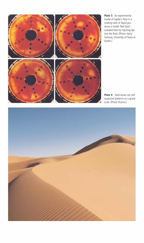
Plate 5 An experimentalmodel of Jupiter’s flow in arotating tank of liquid pro-duces a model ‘Red Spot’,revealed here by injecting dyeinto the fluid. (Photo: HarrySwinney, University of Texas atAustin.)
Plate 6 Sand dunes are self-organized patterns on a grandscale. (Photo: Rosino.)