fitting b-spline curves to point clouds in the presence of ...€¦ · chapter 2. curve fitting of...
TRANSCRIPT

D I P L O M A R B E I T
Fitting B-Spline Curves to Point Clouds inthe Presence of Obstacles
ausgefuhrt am Institut fur
Diskrete Mathematik und Geometrie
der Technischen Universitat Wien
unter Anleitung von o.Univ-Prof. Dr. Helmut Pottmann
durch
Simon Flory
Grafaweg 26710 Nenzing
Datum Unterschrift

Abstract
We consider the computation of an approximating curve to fit a given set of points.Such a curve fitting is a common problem in CAGD and we review three differentapproaches based upon minimization of the squared distance function: the point dis-tance, tangent distance and squared distance error term. We enhance the classic setupcomprising a point cloud and an approximating B-Spline curve by obstacles a finalsolution must not penetrate. Two algorithms for solving the emerging constrainedoptimization problems are presented and used to enclose point clouds from inside aswell as from outside and to avoid arbitrary smooth bounded obstacles. Moreover,approximations of guaranteed quality and shaking objects are examined within thiscontext. In a next step, we extend our work and study the curve fitting problem onparametrized surfaces. The approximation is still performed in the two dimensionalparameter space while geometric properties of the manifold enter the computation atthe same time. Additionally, we use this new error term to approximate the borders ofpoint clouds on manifolds. Finally, as a minimization of the squared distance functionis sensitive to outliers, a curve fitting in the L1 norm based on the signed distancefunction is developed. We describe the necessary results of non-smooth optimizationtheory and apply this robust optimization to curve fitting in the presence of obstacles.

Contents
1 Introduction 1
1.1 Related Work . . . . . . . . . . . . . . . . . . . . . . . . . . . . . . . . . 11.2 Overview . . . . . . . . . . . . . . . . . . . . . . . . . . . . . . . . . . . 21.3 Acknowledgments . . . . . . . . . . . . . . . . . . . . . . . . . . . . . . . 2
2 Curve Fitting of Point Clouds 4
2.1 Introduction . . . . . . . . . . . . . . . . . . . . . . . . . . . . . . . . . . 42.2 Foot Point Computation . . . . . . . . . . . . . . . . . . . . . . . . . . . 52.3 Local Models of the Squared Distance Function . . . . . . . . . . . . . . 7
2.3.1 The Distance Function . . . . . . . . . . . . . . . . . . . . . . . . 72.3.2 Point Distance Minimization . . . . . . . . . . . . . . . . . . . . 82.3.3 Tangent Distance Minimization . . . . . . . . . . . . . . . . . . . 102.3.4 Squared Distance Minimization . . . . . . . . . . . . . . . . . . . 11
2.4 Optimization . . . . . . . . . . . . . . . . . . . . . . . . . . . . . . . . . 142.5 Results . . . . . . . . . . . . . . . . . . . . . . . . . . . . . . . . . . . . . 15
3 Curve Fitting and Obstacles 20
3.1 Constrained Optimization . . . . . . . . . . . . . . . . . . . . . . . . . . 203.1.1 Penalty Method . . . . . . . . . . . . . . . . . . . . . . . . . . . 243.1.2 Active Set Method . . . . . . . . . . . . . . . . . . . . . . . . . . 25
3.2 Applications . . . . . . . . . . . . . . . . . . . . . . . . . . . . . . . . . . 283.2.1 Point Cloud as Obstacle . . . . . . . . . . . . . . . . . . . . . . . 283.2.2 Smooth Obstacles . . . . . . . . . . . . . . . . . . . . . . . . . . 333.2.3 Error Bound Approximation . . . . . . . . . . . . . . . . . . . . 373.2.4 Shaking Objects . . . . . . . . . . . . . . . . . . . . . . . . . . . 39
4 Curve Fitting on Manifolds 41
4.1 Some Elementary Differential Geometry . . . . . . . . . . . . . . . . . . 414.2 Foot Point Computation . . . . . . . . . . . . . . . . . . . . . . . . . . . 444.3 Tangent Distance Minimization on Manifolds . . . . . . . . . . . . . . . 474.4 Results . . . . . . . . . . . . . . . . . . . . . . . . . . . . . . . . . . . . . 47
i

CONTENTS ii
5 Curve Fitting in the L1 Norm 52
5.1 Introduction . . . . . . . . . . . . . . . . . . . . . . . . . . . . . . . . . . 525.2 Non-smooth Optimization . . . . . . . . . . . . . . . . . . . . . . . . . . 54
5.2.1 The Cutting Plane Method . . . . . . . . . . . . . . . . . . . . . 555.3 Results . . . . . . . . . . . . . . . . . . . . . . . . . . . . . . . . . . . . . 57
Bibliography 61
A Splines 63
B B-Spline Curves 68

Chapter 1
Introduction
We consider a set of unstructured points in the plane, forming a model shape suchas an unknown planar curve. Our goal is to approximate this possibly noisy cloud ofpoints by a B-Spline curve P (t) =
∑m
i=0 Bi(t)di. Such a curve fitting of point cloudsis a frequently encountered problem in computational geometry.
The common approach to a solution bases upon an iterative method proposed byHoschek [11] (and recently further developed by [25]). In each iteration the elementsXk of the input point cloud X are assigned a closest point P (tk) on the approximatingcurve. In these foot points, an approximation of the signed or squared distance fromthe curve to the points is minimized.
1.1 Related Work
Usually, curve fitting relies on different local approximations of the squared distancefunction, mainly for the sake of simplicity. A comprehensive review of the differentmethods is given in [28], where the curve fitting problem is further examined from theviewpoint of optimization. The basic point distance minimization, simply measuringthe distance from the foot point to the data point, is widely used in computer aidedgeometric design, e.g. [11, 19, 20, 25]. An improvement taking the distances from thepoints to the tangents in the closest points into account is for example described in[3].
In [21] a quadratic Taylor approximation of the squared distance function is de-veloped. [23] use this local model to approximate smooth target curves with B-Splinecurves. In [28] this squared distance minimization is applied to discrete point clouds.The concepts of curve fitting may be used for surface fitting as well. [29] and [22] arerecent contributions thereto.
The consideration of obstacles in curve design is a widely investigated topic. Con-straints in reverse engineering of classical geometric objects such as lines, circles,spheres and cylinders from point data are studied in [2]. Peters defines SLEVEs [18]and uses them in [17] to construct a spline based curve strictly staying inside a polyg-
1

CHAPTER 1. INTRODUCTION 2
onal channel. In [10] interpolating splines are restricted to manifolds, any obstaclesare avoided by carrying out the interpolation on the distance field of the forbiddenregions. Furthermore, the exact and approximate construction of splines on surfaceswas recently discussed in [24].
In order to overcome the major drawback of the squared distance function’s mini-mization, its sensitivity to outliers, the absolute value of the signed distance functionmay be used in the approximation instead. There is only very few literature availableon this topic. [7] deals with geometric optimization in the L1 norm. In general, non-smooth optimization problems (an L1 norm minimization leads to) are very common,[6, 9, 16] discuss various solutions.
1.2 Overview
The succeeding parts of this work are organized as follows. First, we discuss and com-pare the various methods for curve fitting of point clouds, namely the point, tangentand squared distance minimization.
In chapter 3 we introduce obstacles to the curve fitting problem. We considertwo different kinds of obstacles: the point cloud itself and arbitrary smooth boundedforbidden regions. The emerging constraint optimization problems are solved with apenalty method as well as with an active set method. The results are used to findan alternative approach to the swept volume problem ([27] recently contributed analgorithm thereto) and for a curve approximation of guaranteed quality (a problemaddressed for example in [19]).
The next chapter takes curve fitting from the plane to two dimensional parametricsurfaces. We develop an approximation technique similar to tangent distance min-imization in the plane (compare [3]) by performing the point cloud’s fitting in theparameter space with respect to intrinsic geometric properties of the manifold the ap-proximation is supposed to happen on. In part, results of the previous chapter aregeneralized to enclose point clouds on surfaces with a B-Spline curve.
Chapter 5 sets the comfort of working with the squared distance function aside andsolves the non-smooth optimization problem imposed by applying the signed distancefunction in curve fitting. This approximation in the L1 norm is further examined inthe presence of obstacles.
The appendix summarizes some basic results for polynomial splines and B-Splinecurves.
1.3 Acknowledgments
First and foremost I want to express my gratitude to Professor Helmut Pottmann. Itwas a pleasure to write this thesis under his uncomplicated supervision and with hisvaluable suggestions. Furthermore I seize the chance to thank everyone at the institutecontributing to the development of this work.

CHAPTER 1. INTRODUCTION 3
My sincerest thanks belong to my father and my mother, in the first place for theircommitment to my studies. It’s great to see what the world looks like if the whereand the how long are not subject of discussion. And finally, a Cheers! goes out to allyou other people I spent great times with in the past and will do so in the future.
Chapter 2
Curve Fitting of Point Clouds
2.1 Introduction
The computation of an approximating curve to fit a given set of points is a commonproblem in computer graphics, computer aided geometric design (CAGD) and imageprocessing. In this chapter we introduce the unconstrained curve fitting problem ofpoint clouds and describe a general algorithm to solve it. The subsequent discussion ofthis algorithm takes most parts of this section and focuses on the topics of foot pointcomputation, local approximations of the squared distance function and optimization.Finally, experiments dealing with the obtained results will conclude this first part.
Let X = Xk : k = 0, . . . , n be a given set of points (called the point cloud)representing the shape of an initial curve or the extent of an arbitrary region. In curvefitting, one aims to approximate this set of points by a curve that reflects the originalform of the point cloud in a good way.
B-Spline curves are a common choice for the approximating curve. Assume thedegree of the approximating B-Spline curve is defined a priori. Additionally, the knotsequence and the number of control points are not subject to optimization. Then, theB-Spline curve can be written as
P (t) =
m∑
i=0
Bi(t)di
where Bi(t) describes the basis B-Spline functions of fixed degree and di the controlpoints. It’s convenient to interpret the curve fitting problem as a non-linear opti-mization problem. On optimizing, one asks for a displacement c = (ci)i=0,...,m of thecontrol points di
Pc(t) =
m∑
i=0
Bi(t)(di + ci)
minimizing the distance d(Pc(t), X) of the approximating B-Spline curve to thepoint cloud. In each data point Xk, the error of the approximation is given as the
4
CHAPTER 2. CURVE FITTING OF POINT CLOUDS 5
distance from Xk to a sample point Pc(tk) on the B-Spline curve. Commonly, thissample point is the foot point of Xk on Pc(t) with d(Pc(tk), Xk) = mint ‖Pc(t)−Xk‖.Thus, we define the distance of Pc(t) to X by
d(Pc(t), X) :=n∑
k=0
d(Pc(tk), Xk).
Since it’s favorable to work with sums of squares instead of sums of absolute values,the squared distance function d2(Pc(tk), Xk) is applied instead. Minimizing the sumof distances requires more sophisticated optimization techniques, chapter 5 will dealwith this problem.
In summary, the objective function of the curve fitting problem of point clouds canbe written as
f(c) =
n∑
k=0
d2(Pc(tk), Xk) + λFr(c) (2.1)
where Fr(c) is a regularization term ensuring a smooth solution. The non-linearityof (2.1) suggests an iterative approach to the minimization.
Algorithm 1 (General Curve Fitting). A general algorithm for fitting a B-Splinecurve P (t) to a point cloud X involves the following steps
1. define a suitable start position of the approximating B-Spline curve.
2. assign each data point Xk a parameter value tk, such that P (tk) is the closestpoint of Xk on the approximating B-Spline curve.
3. obtain the objective function f(c) =∑n
k=0 e(Pc(tk), Xk) + λFr(c) of the opti-mization problem, where e(Pc(tk), Xk) is a local approximation of the squareddistance function.
4. get the displacement c of the control points by minimizing f(c).
5. displace the control points of the approximating B-Spline curve. If the updatedcurve approximates the given point cloud reasonably good, stop.
6. otherwise, continue with step 2.
In the following, steps 2 to 4 will be discussed in detail.
2.2 Foot Point Computation
Step 2 of algorithm 1 determines the sample points on the approximating B-Splinecurve where the curve’s distance to the point cloud is measured in. As mentionedbefore, these sample points are chosen to be the foot points of the data points on theB-Spline curve.
CHAPTER 2. CURVE FITTING OF POINT CLOUDS 6
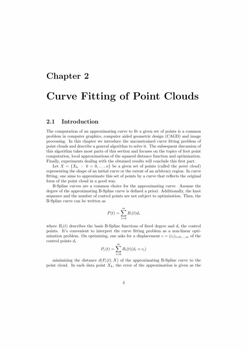
p
c(t∗)c(t∗)
c(t)
Figure 2.1: Geometric interpretation of the foot point computation problem in R2.
Let c(t) : R → Rk be a parametric curve and p a point of R
k. The closest point ofp on c(t) minimizes
g(t) = ‖c(t) − p‖2 = (c(t) − p)2. (2.2)
For a minimizer t∗ of g(t), c(t∗) is called the foot point of p on c(t).We minimize (2.2) with a Newton iteration. Let ti be the current iterate. The idea
of the Newton iteration is to work with a quadratic Taylor approximation of g in ti
gi(t) = g(ti) + ∇g(ti)T (t − ti) +1
2(t − ti)T∇2g(ti)(t − ti) + o(t3).
A necessary condition for a minimum of gi(t) is the vanishing of the gradient
∇gi(t) = ∇g(ti) + ∇2g(ti)(t − ti) = 0
The next iterate ti+1 = ti + δi is obtained by solving this expression for t. The updatein the i-th Newton iteration turns out to be
δi = −[∇2g(ti)
]−1· ∇g(ti).
In order to improve the convergence behavior of the Newton iteration we do not simplyupdate with δi but reduce the step length in direction of δi by a factor λ
ti+1 = ti + λδi.
A possible choice for λ is according to the successive reduction rule. For given β ∈ (0, 1)we set λ = βm for the smallest m ∈ N with g(ti + βmδi) < g(ti).
For the foot point computation problem in curve fitting, a starting point of theNewton iteration could be obtained by sampling the curve sufficiently dense and usingthe closest sample point to p. For the sake of simplicity we multiply g(t) in (2.2) with12 and get as update
δi = −(c(ti) − p) · c(ti)
c2(ti) + (c(ti) − p) · c(ti).
CHAPTER 2. CURVE FITTING OF POINT CLOUDS 7
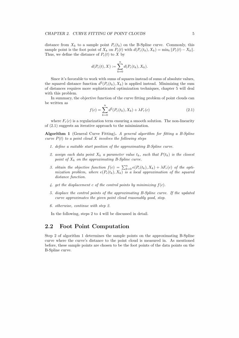
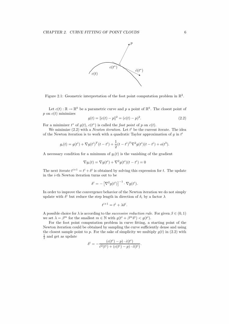
Figure 2.2: Medial axis for a closed curve with certain inscribed circles.
The Newton iteration is aborted if either the update δi is smaller than a certainthreshold or the number of iterations exceeds a predefined value.
In a geometric interpretation, a necessary condition for a foot point is, as statedabove, the vanishing of the first derivative
d
dtg(t) = (c(t) − p) · c(t) = 0.
Thus, the connecting line from p to the foot point has to be perpendicular to thetangent in the foot point, as shown in figure 2.1.
2.3 Local Models of the Squared Distance Function
2.3.1 The Distance Function
As pointed out in the introduction of this chapter, the (squared) distance functionplays an important role in curve fitting. Given a curve c(t) in the plane, the distancefunction
d(x) := minp∈c(t)
|p − x|
assigns each point x ∈ R2 the shortest distance to c(t). As a matter of fact, the
distance function is not differentiable on c(t).The signed distance function overcomes this problem. It is defined as the viscosity
solution of the Eikonal equation.
Definition 2.1. d is the signed distance function of a curve d(x) = 0 if
∇d2 = 1 or ‖∇d‖ = 1
holds, respectively.

CHAPTER 2. CURVE FITTING OF POINT CLOUDS 8
Casually speaking, the signed distance function assigns each point’s unsigned dis-tance a sign, according to the side of the curve the point is located at. In the following,if not stated otherwise, we use the term ”distance function” for the signed distancefunction, too.
Again, the signed distance function is not differentiable everywhere. It is singularin points of the medial axis. The medial axis is defined as the locus of the center of allmaximal inscribed disks of an object. Figure 2.2 illustrates the medial axis of a closedcurve.
The level sets of the distance function are the offsets from the curve c(t) which areof importance in various fields of computational geometry.
In the literature on partial differential equations, requirements for the existenceand uniqueness of a solution of the Eikonal equation are well known. However, it isnot very feasible to apply this theory to the problem of curve fitting directly. Insteadof aiming to compute the fitting curve’s exact distance function, approximations areused.
For the sake of simplicity, the curve fitting presented in this chapter is based onapproximations of the squared distance function. A possible way would be to discretizethe computation of the squared distance function on a grid. Tsai’s algorithm [26]realizes this. Though we will use Tsai’s algorithm later on when we require distancefields from obstacles in the plane, it is not applicable in general. Since we formulatedthe curve fitting problem as an optimization problem, we are in need of an analyticrepresentation of any approximation of the signed distance function.
Instead of using a discretization, we work with local models of the squared signeddistance function. In the following, three approaches to measure the squared distanceof a point to a curve in an approximate way are presented: point distance minimization,tangent distance minimization and squared distance minimization.
All three error terms are concrete realizations of step 3 of the general curve fittingalgorithm. Thus, the foot points P (tk) for each data point Xk are already available atthis stage of the discussion.
2.3.2 Point Distance Minimization
Point distance minimization is the first method we are going to study in our review oflocal models of a curve’s squared distance function. It goes back to a work by Hoscheck[11]. There, the author assigns each data point Xk a parameter value tk (a foot point)and then uses ‖Pc(tk) − Xk‖
2 as approximation of the squared distance function inthe optimization’s objective function. Similar to the general curve fitting algorithmHoschek repeats this parametrization and minimization iteratively. The method iscalled intrinsic parametrization for approximation originally.
We might call this curve fitting approach based on the error term
ePDM,k(c) = ‖Pc(tk) − Xk‖2
point distance minimization or short PDM for consistency with the naming of theother methods. In order to use ePDM,k in a computational implementation, we write

CHAPTER 2. CURVE FITTING OF POINT CLOUDS 9
(a) Initial setup (b) Final approximation after 20 iterations
Figure 2.3: Curve fitting with PDM.
it as a quadratic function ePDM,k(c) = cT · APDM · c + 2 · bTPDM · c + kPDM , where
c =
(c0
...cm
)summarizes the single displacements of the control points into a single
vector c ∈ R2m+2.
We expand
ePDM,k(c) = ‖Pc(tk) − Xk‖2 =
[m∑
i=0
Bi(tk)(di + ci) − Xk
]2
and collect the powers of the unknown displacement c. By doing so, we get
(APDM )2i...2i+1,2j...2j+1
= Bi(tk)Bj(tk) · I2 0 ≤ i, j ≤ m
where I2 denotes the two dimensional identity matrix. Moreover,
(bPDM )2i...2i+1 = Bi(tk) · (P (tk) − Xk) 0 ≤ i ≤ m
andkPDM = (P (tk) − Xk)2.
Point distance minimization is very popular in computer aided geometric design. Thismight be due the simplicity of this approach as it just replaces P (t) in (2.1) with P (tk).However, if we consider that the foot points depend on the variable control points, wemay expect that ePDM doesn’t serve too well as approximation of the squared distancefunction. Indeed, the convergence of PDM is slow as upcoming experiments will show.
The poor convergence rate of the point distance minimization algorithm is approvedby the authors of [28] theoretically. There, curve fitting algorithms are studied as nativeoptimization algorithms in the context of the non-linear least squares problem of (2.1).That work shows, that PDM is a variant of the steepest descent method which enjoysonly linear convergence.
CHAPTER 2. CURVE FITTING OF POINT CLOUDS 10
(a) Initial setup (b) Final approximation after 15 iterations
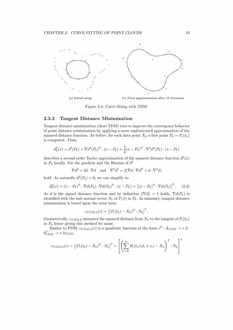
Figure 2.4: Curve fitting with TDM.
2.3.3 Tangent Distance Minimization
Tangent distance minimization (short TDM) tries to improve the convergence behaviorof point distance minimization by applying a more sophisticated approximation of thesquared distance function. As before, for each data point Xk a foot point Pk = Pc(tk)is computed. Then,
d2k(x) = d2(Pk) + ∇d2(Pk)T · (x − Pk) +
1
2(x − Pk)T · ∇2d2(Pk) · (x − Pk)
describes a second order Taylor approximation of the squared distance function d2(x)in Pk locally. For the gradient and the Hessian of d2
∇d2 = 2d · ∇d and ∇2d2 = 2(∇d · ∇dT + d · ∇2d)
hold. As naturally d2(Pk) = 0, we can simplify to
d2k(x) = (x − Pk)T · ∇d(Pk) · ∇d(Pk)T · (x − Pk) =
[(x − Pk)T · ∇d(Pk)
]2. (2.3)
As d is the signed distance function and by definition ‖∇d‖ = 1 holds, ∇d(Pk) isidentified with the unit normal vector Nk of Pc(t) in Pk. In summary, tangent distanceminimization is based upon the error term
eTDM,k(c) =[(Pc(tk) − Xk)T · Nk
]2.
Geometrically, eTDM,k measures the squared distance from Xk to the tangent of Pc(tk)in Pk hence giving this method its name.
Similar to PDM, eTDM,k(c) is a quadratic function of the form cT · ATDM · c + 2 ·bTTDM · c + kTDM .
eTDM,k(c) =[(Pc(tk) − Xk)T · Nk
]2=
(
m∑
i=0
Bi(tk)(di + ci) − Xk
)T
· Nk
2
CHAPTER 2. CURVE FITTING OF POINT CLOUDS 11
is transformed and summarized to
(ATDM )2i...2i+1,2j...2j+1
= Bi(tk)Nk · NTk Bj(tk) 0 ≤ i, j ≤ m
(bTDM )2i...2i+1 = dkBi(tk) · Nk 0 ≤ i ≤ m
andkTDM = d2
k
where dk := (P (tk) − Xk)T · Nk.Though not as popular as PDM, TDM is widely used in CAGD. And indeed, it
shows faster convergence than the point distance minimization method. However,approximating a curve by its tangent for measuring the distance might be insufficient.This comes especially true if Xk is far from the curve or close to a high curvaturepoint. Additionally, TDM not only holds the foot points fixed when displacing thecontrol points but also leaves out to update the tangents. These drawbacks make TDMunstable.
Again, the work in [28] rates TDM from the viewpoint of optimization. TDM turnsout to be a Gauss-Newton method, fortifying our assumption of a mostly improvedconvergence behavior compared to the point distance minimization. Optimizationtheory knows about the instability issues of the Gauss-Newton method and proposesseveral improvements such as the damped Gauss-Newton method or the Levenberg-Marquart method. We want to discuss a variant of the damped Gauss-Newton methodin detail.
The following approach is based upon the successive reduction rule, already dis-cussed in conjunction with the foot point computation. Instead of updating the B-Spline curve’s control points with the full displacement obtained from minimizing (2.1),a step length controlled update is done
dj+1 = dj + λcj .
According to the successive reduction rule, we choose β ∈ (0, 1) and set λ = βm
for the smallest m ∈ N with g(dj+1) < g(dj). Hereby, g describes the error of theapproximation for the current choice of dj+1, that is
g(dj+1) =
n∑
k=0
(
m∑
i=0
Bi(tk)dj+1i − Xk
)T
· Nk
2
.
The combination of the successive reduction rule and TDM improves the stabilityof TDM effectively; we will call it damped tangent distance minimization conveniently.
2.3.4 Squared Distance Minimization
Squared distance minimization (abbreviated SDM) is the third and last error term inour discussion of local models of the squared distance function. SDM aims to over-come the shortcomings of TDM by incorporating information about the approximatingcurve’s curvature.
CHAPTER 2. CURVE FITTING OF POINT CLOUDS 12
Nk
Tk(0, ρ)
(0, d)
Pc(t)
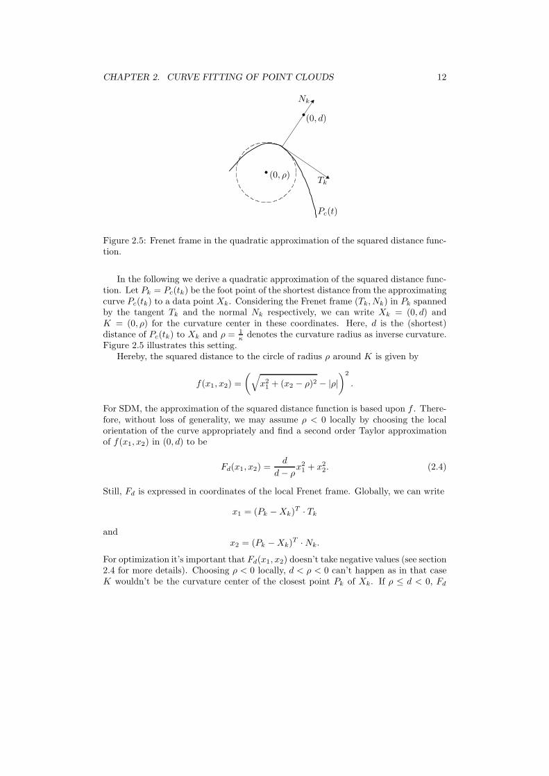
Figure 2.5: Frenet frame in the quadratic approximation of the squared distance func-tion.
In the following we derive a quadratic approximation of the squared distance func-tion. Let Pk = Pc(tk) be the foot point of the shortest distance from the approximatingcurve Pc(tk) to a data point Xk. Considering the Frenet frame (Tk, Nk) in Pk spannedby the tangent Tk and the normal Nk respectively, we can write Xk = (0, d) andK = (0, ρ) for the curvature center in these coordinates. Here, d is the (shortest)distance of Pc(tk) to Xk and ρ = 1
κdenotes the curvature radius as inverse curvature.
Figure 2.5 illustrates this setting.Hereby, the squared distance to the circle of radius ρ around K is given by
f(x1, x2) =
(√x2
1 + (x2 − ρ)2 − |ρ|
)2
.
For SDM, the approximation of the squared distance function is based upon f . There-fore, without loss of generality, we may assume ρ < 0 locally by choosing the localorientation of the curve appropriately and find a second order Taylor approximationof f(x1, x2) in (0, d) to be
Fd(x1, x2) =d
d − ρx2
1 + x22. (2.4)
Still, Fd is expressed in coordinates of the local Frenet frame. Globally, we can write
x1 = (Pk − Xk)T · Tk
andx2 = (Pk − Xk)T · Nk.
For optimization it’s important that Fd(x1, x2) doesn’t take negative values (see section2.4 for more details). Choosing ρ < 0 locally, d < ρ < 0 can’t happen as in that caseK wouldn’t be the curvature center of the closest point Pk of Xk. If ρ ≤ d < 0, Fd
CHAPTER 2. CURVE FITTING OF POINT CLOUDS 13
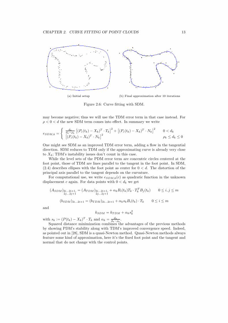
(a) Initial setup (b) Final approximation after 10 iterations
Figure 2.6: Curve fitting with SDM.
may become negative; thus we will use the TDM error term in that case instead. Forρ < 0 < d the new SDM term comes into effect. In summary we write
eSDM,k =
dk
dk−ρk
[(Pc(tk) − Xk)T · Tk
]2+[(Pc(tk) − Xk)T · Nk
]20 < dk[
(Pc(tk) − Xk)T · Nk
]2ρk ≤ dk ≤ 0
One might see SDM as an improved TDM error term, adding a flow in the tangentialdirection. SDM reduces to TDM only if the approximating curve is already very closeto Xk; TDM’s instability issues don’t count in this case.
While the level sets of the PDM error term are concentric circles centered at thefoot point, those of TDM are lines parallel to the tangent in the foot point. In SDM,(2.4) describes ellipses with the foot point as center for 0 < d. The distortion of theprincipal axis parallel to the tangent depends on the curvature.
For computational use, we write eSDM,k(c) as quadratic function in the unknowndisplacement c again. For data points with 0 < dk we get
(ASDM )2i...2i+1,2j...2j+1
= (ATDM )2i...2i+1,2j...2j+1
+ αkBi(tk)Tk · T Tk Bj(tk) 0 ≤ i, j ≤ m
(bSDM )2i...2i+1 = (bTDM )2i...2i+1 + αkskBi(tk) · Tk 0 ≤ i ≤ m
andkSDM = kTDM + αks2
k
with sk := (P (tk) − Xk)T · Tk and αk = dk
dk−ρk.
Squared distance minimization combines the advantages of the previous methodsby showing PDM’s stability along with TDM’s improved convergence speed. Indeed,as pointed out in [28], SDM is a quasi-Newton method. Quasi-Newton methods alwaysfeature some kind of approximation, here it’s the fixed foot point and the tangent andnormal that do not change with the control points.
CHAPTER 2. CURVE FITTING OF POINT CLOUDS 14
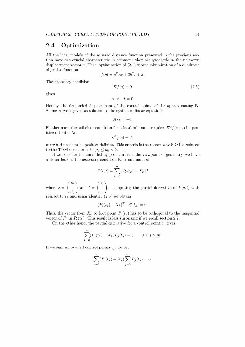
2.4 Optimization
All the local models of the squared distance function presented in the previous sec-tion have one crucial characteristic in common: they are quadratic in the unknowndisplacement vector c. Thus, optimization of (2.1) means minimization of a quadraticobjective function
f(c) = cT Ac + 2bT c + d.
The necessary condition∇f(c) = 0 (2.5)
givesA · c + b = 0.
Hereby, the demanded displacement of the control points of the approximating B-Spline curve is given as solution of the system of linear equations
A · c = −b.
Furthermore, the sufficient condition for a local minimum requires ∇2f(x) to be pos-itive definite. As
∇2f(c) = A,
matrix A needs to be positive definite. This criteria is the reason why SDM is reducedto the TDM error term for ρk ≤ dk < 0.
If we consider the curve fitting problem from the viewpoint of geometry, we havea closer look at the necessary condition for a minimum of
F (c, t) =
n∑
k=0
‖Pc(tk) − Xk‖2
where c =
(c0
...cm
)and t =
(t0
...tn
). Computing the partial derivative of F (c, t) with
respect to tk and using identity (2.5) we obtain
(Pc(tk) − Xk)T · P ′c(tk) = 0.
Thus, the vector from Xk to foot point Pc(tk) has to be orthogonal to the tangentialvector of Pc in Pc(tk). This result is less surprising if we recall section 2.2.
On the other hand, the partial derivative for a control point cj gives
n∑
k=0
(Pc(tk) − Xk)Bj(tk) = 0 0 ≤ j ≤ m.
If we sum up over all control points cj , we get
n∑
k=0
(Pc(tk) − Xk)
m∑
j=0
Bj(tk) = 0.

CHAPTER 2. CURVE FITTING OF POINT CLOUDS 15
Due to the convex hull property of B-Spline curves,∑m
j=0 Bj(tk) = 1 holds (compareappendix B) and we finally see
n∑
k=0
(Pc(tk) − Xk) = 0.
If we interpret the vectors from Xk to Pc(tk) as forces acting on the approximatingcurve, a solution of the curve fitting problem means finding a curve where these forcesare in equilibrium. Again, this identity could be expected for this scenario as we dealwith the curve fitting problem by means of a least square problem.
2.5 Results
The objective function in (2.1) includes an additional term called a regularization orsmoothing term. Its purpose is to avoid a degeneration of the approximating curvewhen fitting the point cloud. On the one hand
Fr1(c) =
∫
P
‖P ′c(t)‖
2dt
minimizes the L2 norm of the first derivative keeping the length of the approximatingcurve small, whereas
Fr2(c) =
∫
P
‖P ′′c (t)‖2dt
on the other hand measures the bending energy of Pc(t) and prevents the creation ofloops in a minimization.
Again, for a software implementation, these smoothing terms are written as qua-dratic functions cT · As · c + 2 · bT
s · c + ks. For Frk(c) (k = 1, 2) we get
(As)2i...2i+1,2j...2j+1
= vij · I2 0 ≤ i, j ≤ m
(bs)2i...2i+1 =m∑
j=0
vij · dj 0 ≤ i ≤ m
ks =
m∑
i=0
m∑
j=0
vijdj
T
· di
with vij =∫
PB
(k)i (t)B
(k)j (t)dt. The integrals could be evaluated in a numerical inte-
gration based on the parameter values tk of the foot points.For the following results only the second smoothing term Fr2(c) was applied,
weighted with a factor λ. Usually, λ was set to be 10−4 in the beginning and washalved at each iteration step. If factor λ is different from this value we mention thisin the description of the corresponding experiment.
CHAPTER 2. CURVE FITTING OF POINT CLOUDS 16
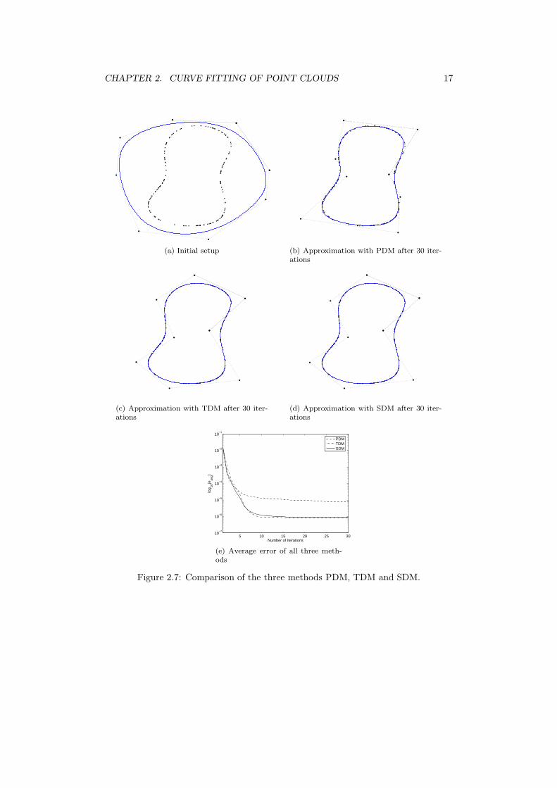
The point clouds used throughout this work were created according to the samemethod. At first, an auxiliary B-Spline curve is defined. This curve is randomlysampled in a given number of points, the distribution of the samples’ parameter valuesis chosen to be uniform. In each of these sample points an element of the point cloudis given in random distance from the curve in the direction of the normal vector. Thedistances are usually drawn from a normal distribution.
For some experiments, the error of the computed approximation is visualized in achart. This error is chosen to be the average squared distance of the curve to the pointcloud
eavg =1
n + 1
n∑
i=0
‖P (tk) − Xk‖2
whereas P (tk) is the foot point of Xk on the approximating B-Spline curve. The erroris plotted on a logarithmic scaled axis versus the corresponding number of iterations.
Figures 2.3, 2.4 and 2.6 show the results of a PDM, TDM and SDM based curvefitting respectively. The point cloud gets more noisier and more complex throughoutthe examples, illustrating the way curve fitting works with the presented algorithms.However, these figures do not compare the methods directly - this is done in figures2.7 and 2.8.
The first comparison visualizes the point cloud’s approximation after 30 iterationsof each algorithm. By eye it is possible to see that PDM gives the worst final resultwhile TDM and SDM seem to perform equally. This first impression is confirmedby the error chart showing comparable convergence for tangent and squared distanceminimization while the point distance minimization method fits the data much moreslowly.
The second comparison focuses on TDM’s stability issues. For this experiment, nosuccessive reduction rule was applied in tangent distance minimization. This algorithmgets trapped in a local minimum, while PDM and SDM both fit the point cloud withgood quality. PDM converges slower than SDM but seems to give a slightly bettersolution after 100 iterations.
Finally an experiment examines the effects of the successive reduction rule. Whilethe standard TDM method fails to converge for the setup in figure 2.9, the dampedTDM algorithm shows a good and stable convergence behavior. Applying the succes-sive reduction rule to PDM and SDM didn’t mean any improvement.
CHAPTER 2. CURVE FITTING OF POINT CLOUDS 17
(a) Initial setup (b) Approximation with PDM after 30 iter-ations
(c) Approximation with TDM after 30 iter-ations
(d) Approximation with SDM after 30 iter-ations
5 10 15 20 25 3010
−7
10−6
10−5
10−4
10−3
10−2
10−1
Number of Iterations
log 10
(eav
g)
PDMTDMSDM
(e) Average error of all three meth-ods
Figure 2.7: Comparison of the three methods PDM, TDM and SDM.
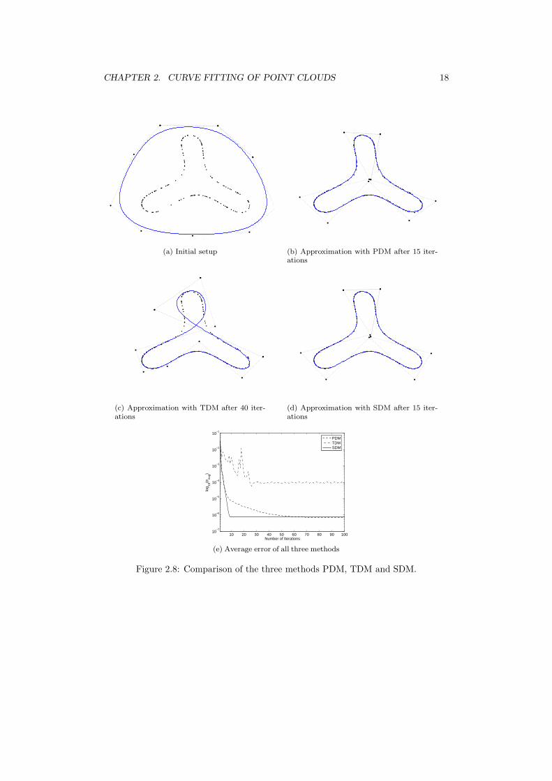
CHAPTER 2. CURVE FITTING OF POINT CLOUDS 18
(a) Initial setup (b) Approximation with PDM after 15 iter-ations
(c) Approximation with TDM after 40 iter-ations
(d) Approximation with SDM after 15 iter-ations
10 20 30 40 50 60 70 80 90 10010
−7
10−6
10−5
10−4
10−3
10−2
10−1
Number of Iterations
log 10
(eev
g)
PDMTDMSDM
(e) Average error of all three methods
Figure 2.8: Comparison of the three methods PDM, TDM and SDM.

CHAPTER 2. CURVE FITTING OF POINT CLOUDS 19
(a) Initial setup (b) Final approximation with damped TDMafter 30 iterations
0 5 10 15 20 25 3010
−2
10−1
100
101
102
103
104
105
106
Number of Iterations
log 10
(eav
g)
TDM
damped TDM
(c) Average error of TDM and dam-ped TDM
Figure 2.9: Improved convergence of damped TDM.

Chapter 3
Curve Fitting and Obstacles
Chapter 2 described the classical curve fitting problem for point clouds and presentedthree methods to approximate data points with a B-Spline curve. In this chapter wewant to go a step further and examine curve fitting of point clouds in the presence ofobstacles: besides the set of data points and the starting position of the approximatingcurve regions are defined the final solution must not penetrate.
Technically, curve fitting in the consideration of obstacles poses a constrained op-timization problem (while the minimization of chapter 2 was unconstrained). Thegeneral curve fitting algorithm 1 will still be applicable, only the optimization in step4 will be of a different kind.
In the beginning some theory on constrained optimization will be introduced. Then,two approaches for finding a solution of a constrained problem will be studied and willbe applied to two general curve fitting problems in the presence of obstacles. Finally,some applications are sketched.
3.1 Constrained Optimization
Given a non empty set X ⊆ Rn and a function f : X → R constrained optimization is
aboutmin f(x) subject to x ∈ X. (3.1)
Similar to unconstrained problems we may focus without loss of generality only onminimization as
maxx∈X
f(x) = minx∈X
−f(x).
The set X is called the feasible region and is usually defined by a collection of equalityand inequality constraints
min f(x) subject to gi(x) ≤ 0 1 ≤ i ≤ p
hj(x) = 0 1 ≤ j ≤ q.(3.2)
20
CHAPTER 3. CURVE FITTING AND OBSTACLES 21
We will see that curve fitting in the presence of obstacles can be formulated as anoptimization problem with only linear constraints
min f(x) subject to aTi x ≤ αi 1 ≤ i ≤ p
bTj x = βj 1 ≤ j ≤ q.
(3.3)
Thus, the theory discussion in the remaining parts of this section concentrates mostlyon the linear constrained case.
Definition 3.1. For the minimization problem of (3.1)
(i) a vector x ∈ Rn is called feasible if x ∈ X.
(ii) a feasible vector x∗ ∈ Rn is called a global minimum if
f(x∗) ≤ f(x) ∀x ∈ X
Analogous, local, strict global and strict local minima are defined as for the uncon-strained case.
In optimization, convex functions play an important role.
Definition 3.2. A function f : Rn → R is called convex if
f(αx + (1 − α)y) ≤ αf(x) + (1 − α)f(y) ∀ x, y ∈ Rn, α ∈ (0, 1)
An optimization problem is called a convex optimization problem if its objective func-tion is convex.
Example 3.1. Let q(x) = 12xT Ax+ bT x+ c be a quadratic form. Then q(x) is convex
if and only if A is positive semi-definite, because
f(αx + (1 − α)y) =
1
2αxT Ax +
1
2(1 − α)yT Ay −
1
2α(1 − α)(x − y)T A(x − y) + αbT x + (1 − α)bT y + c
≤ αf(x) + (1 − α)f(y)
since α > 0, (1 − α) > 0 and (x − y)T A(x − y) ≥ 0 only if A is positive semi-definite.
Definition 3.3 (Lagrange Function). The function L : Rn × R
p × Rq → R,
L(x, λ, µ) := f(x) +
p∑
i=1
λigi(x) +
q∑
j=1
µjhj(x)
is called the Lagrange Function of the constrained optimization problem (3.2).
The Lagrange Function is used in the definition of the fundamental Karush-Kuhn-Tucker conditions.

CHAPTER 3. CURVE FITTING AND OBSTACLES 22
∇f∇h
f
h(x)=0
Figure 3.1: Visualization of the KKT conditions.
Definition 3.4 (KKT conditions). For the optimization problem of (3.2) with f , gi
and hj ∈ C1 for i = 1, . . . , p and j = 1, . . . , q
(i) the conditions
∇xL(x, λ, µ) = 0
λi ≥ 0, gi(x) ≤ 0, λigi(x) = 0
hj(x) = 0
are called Karush-Kuhn-Tucker conditions (KKT conditions).
(ii) A triple (x∗, λ∗, µ∗) ∈ Rn×R
p×Rq meeting the KKT conditions is called Karush-
Kuhn-Tucker point (KKT point). λ∗ and µ∗ are called the Lagrange Multipliers.
Example 3.2. For a minimization problem with a single equality constraint
min f(x) subject to h(x) = 0
the KKT conditions ask for the gradients ∇f and ∇h to be linear dependent
∇xL(x, λ, µ) = ∇f(x) + λ∇h(x) = 0.
If we interpret the constraint as set of possible solutions, the minimum is found whereh has first order contact with a level set of f . This example is visualized in figure 3.1.
The KKT conditions demand λi ≥ 0, gi(x) ≤ 0, λigi(x) = 0. Thus, in a KKT point(x∗, λ∗, µ∗) either λ∗
i or gi(x∗) is zero. It’s convenient to summarize the indices of the
active inequalities inI(x∗) := i : gi(x
∗) = 0.
The KKT conditions reduce to ∇f(x) = 0 if there are no constraints. That’swhy one may expect the KKT conditions to play an important role when formulatingnecessary conditions for minimas in constrained optimization.
Results for necessary conditions in constrained optimization make use of Farkas’Lemma.
CHAPTER 3. CURVE FITTING AND OBSTACLES 23
Lemma 3.1 (Farkas). For A ∈ Rm×n and c ∈ R
n one and only one of the followingtwo systems has a solution
(i) A · x ≤ 0 and cT · x > 0 for x ∈ Rn
(ii) AT · y = c and y ≥ 0 for y ∈ Rm
Proof. A proof of Farkas’ lemma is omitted here. It can be found for example in[6].
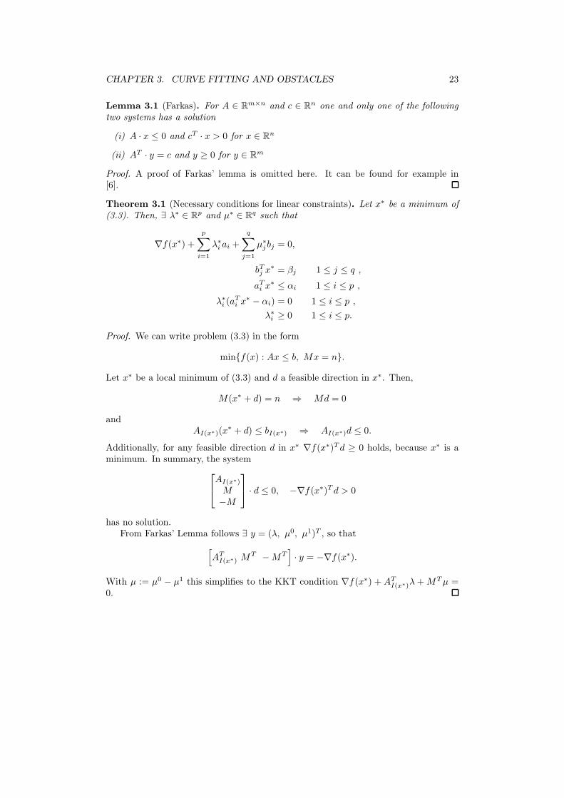
Theorem 3.1 (Necessary conditions for linear constraints). Let x∗ be a minimum of(3.3). Then, ∃ λ∗ ∈ R
p and µ∗ ∈ Rq such that
∇f(x∗) +
p∑
i=1
λ∗i ai +
q∑
j=1
µ∗jbj = 0,
bTj x∗ = βj 1 ≤ j ≤ q ,
aTi x∗ ≤ αi 1 ≤ i ≤ p ,
λ∗i (a
Ti x∗ − αi) = 0 1 ≤ i ≤ p ,
λ∗i ≥ 0 1 ≤ i ≤ p.
Proof. We can write problem (3.3) in the form
minf(x) : Ax ≤ b, Mx = n.
Let x∗ be a local minimum of (3.3) and d a feasible direction in x∗. Then,
M(x∗ + d) = n ⇒ Md = 0
andAI(x∗)(x
∗ + d) ≤ bI(x∗) ⇒ AI(x∗)d ≤ 0.
Additionally, for any feasible direction d in x∗ ∇f(x∗)T d ≥ 0 holds, because x∗ is aminimum. In summary, the system
AI(x∗)
M−M
· d ≤ 0, −∇f(x∗)T d > 0
has no solution.From Farkas’ Lemma follows ∃ y = (λ, µ0, µ1)T , so that
[AT
I(x∗) MT − MT]· y = −∇f(x∗).
With µ := µ0 − µ1 this simplifies to the KKT condition ∇f(x∗) + ATI(x∗)λ + MT µ =
0.

CHAPTER 3. CURVE FITTING AND OBSTACLES 24
Given non-linear constraints, additional regularity requirements are necessary toformulate necessary conditions for minima on top of the KKT conditions.
Theorem 3.2. Let (x∗, λ∗, µ∗) ∈ Rn × R
p × Rq be a KKT point of the convex opti-
mization problem
min f(x) subject to gi(x) ≤ 0 1 ≤ i ≤ p
bTj x = βi 1 ≤ i ≤ q
(3.4)
whereas f and gi are continuous differentiable convex functions. Then, x∗ is a mini-mum of (3.4).
Proof. Assume x is a feasible point of (3.4). Then, the convexity of f and the KKTconditions give for any feasible x ∈ R
n
f(x) ≥ f(x∗) + ∇f(x∗)T (x − x∗)
= f(x∗) −
p∑
i=1
λ∗i ∇gi(x
∗)T (x − x∗) −
q∑
j=1
µ∗jb
Tj (x − x∗)
= f(x∗) −∑
i∈I(x∗)
λ∗i ∇gi(x
∗)T (x − x∗)
≥ f(x∗)
becauseλ∗
i∇gi(x∗)T (x − x∗) ≤ λ∗
i gi(x) − λ∗i gi(x
∗) = λ∗i gi(x) ≤ 0
as λ∗i ≥ 0, gi(x) ≤ 0 in x and gi convex for i ∈ I(x∗).
The last two results summarized give the equivalency of the KKT conditions withthe solution of a convex optimization problem with linear constraints.
Corollary 3.1. Given the convex optimization problem of (3.4) whereas all constraintsare linear, x∗ is a minimum of (3.4) if and only if Lagrange Multipliers λ∗ ∈ R
p andµ∗ ∈ R
q exist such that (x∗, λ∗, µ∗) is a KKT point of (3.4).
After some basic theory on constrained optimization we turn our focus on twomethods to solve constrained optimization problems: the penalty method and theactive set method.
3.1.1 Penalty Method
Penalty methods are classical techniques to solve constrained optimization problemsof the form
min f(x) subject to hj(x) = 0 1 ≤ i ≤ q.
Their basic idea is to deal with the given constrained problem by a series of un-constrained problems which punish forbidden solutions more and more by adding aweighted penalty term to the original objective function
P (x, αk) = f(x) + αkr(x),
CHAPTER 3. CURVE FITTING AND OBSTACLES 25
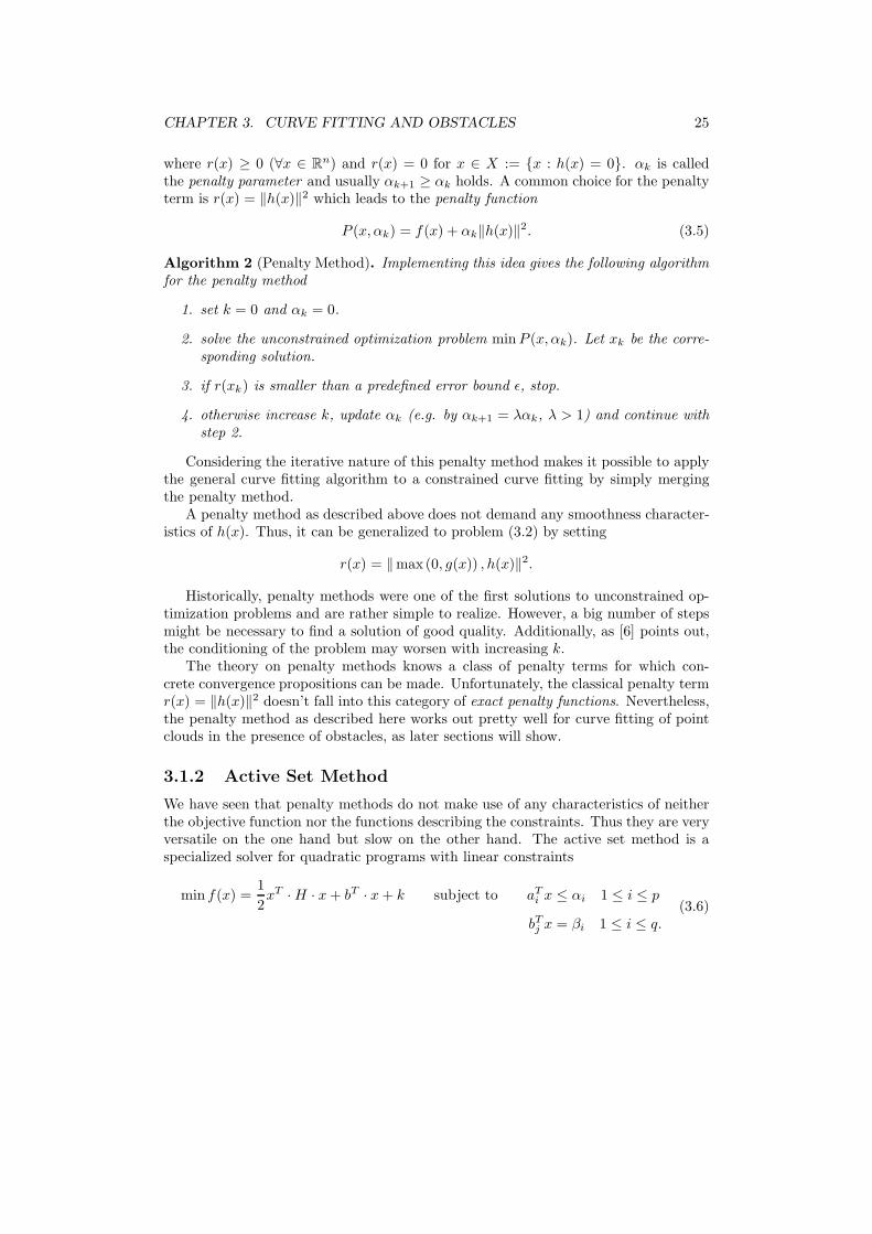
where r(x) ≥ 0 (∀x ∈ Rn) and r(x) = 0 for x ∈ X := x : h(x) = 0. αk is called
the penalty parameter and usually αk+1 ≥ αk holds. A common choice for the penaltyterm is r(x) = ‖h(x)‖2 which leads to the penalty function
P (x, αk) = f(x) + αk‖h(x)‖2. (3.5)
Algorithm 2 (Penalty Method). Implementing this idea gives the following algorithmfor the penalty method
1. set k = 0 and αk = 0.
2. solve the unconstrained optimization problem min P (x, αk). Let xk be the corre-sponding solution.
3. if r(xk) is smaller than a predefined error bound ǫ, stop.
4. otherwise increase k, update αk (e.g. by αk+1 = λαk, λ > 1) and continue withstep 2.
Considering the iterative nature of this penalty method makes it possible to applythe general curve fitting algorithm to a constrained curve fitting by simply mergingthe penalty method.
A penalty method as described above does not demand any smoothness character-istics of h(x). Thus, it can be generalized to problem (3.2) by setting
r(x) = ‖max(0, g(x)) , h(x)‖2.
Historically, penalty methods were one of the first solutions to unconstrained op-timization problems and are rather simple to realize. However, a big number of stepsmight be necessary to find a solution of good quality. Additionally, as [6] points out,the conditioning of the problem may worsen with increasing k.
The theory on penalty methods knows a class of penalty terms for which con-crete convergence propositions can be made. Unfortunately, the classical penalty termr(x) = ‖h(x)‖2 doesn’t fall into this category of exact penalty functions. Nevertheless,the penalty method as described here works out pretty well for curve fitting of pointclouds in the presence of obstacles, as later sections will show.
3.1.2 Active Set Method
We have seen that penalty methods do not make use of any characteristics of neitherthe objective function nor the functions describing the constraints. Thus they are veryversatile on the one hand but slow on the other hand. The active set method is aspecialized solver for quadratic programs with linear constraints
min f(x) =1
2xT · H · x + bT · x + k subject to aT
i x ≤ αi 1 ≤ i ≤ p
bTj x = βi 1 ≤ i ≤ q.
(3.6)

CHAPTER 3. CURVE FITTING AND OBSTACLES 26
In the following, the active set algorithm is described, a detailed discussion is appended.For the method’s description, some notation is needed. As before, I(xk) := i :aT
i xk = αi is the set of active inequalities for the current iterate xk, giving themethod its name. In addition we write
Ak :=
...aT
i ∀ i ∈ I(xk)...
and B :=
bT1...
bTq
.
Algorithm 3 (Active Set Method). The active set method for linear constrainedquadratic programs involves the following steps
1. choose a feasible point x0 of (3.6). Set λ0 ∈ Rp and µ0 ∈ R
q to be the corre-sponding Lagrange Multipliers and I0 := i : aT
i x0 = αi, k := 0.
2. if (xk, λk, µk) is a KKT point, stop.
3. for i /∈ Ik set λki := 0. Compute (xk, λk+1
Ik, µk+1) as solution of the system of
linear equations
H AT
k BT
Ak 0 0B 0 0
·
xλIk
µ
=
−∇f(xk)
00
.
4. (a) if xk = 0 and λk+1i ≥ 0 (∀i ∈ Ik), stop.
(b) if xk = 0 and mini∈Ikλk+1
i < 0, compute index j as λk+1j = mini∈Ik
λk+1i
and set
xk+1 := xk
Ik+1 := Ik\j.
Continue with step 5.
(c) if xk 6= 0 and xk+1 := xk +xk is a feasible point of (3.6), set Ik+1 := Ik
and continue with step 5.
(d) if xk 6= 0 and xk+1 := xk + xk is not feasible, compute index r as
αr − aTr xk
aTr xk
= min
αi − aT
i xk
aTi xk
∣∣∣ i /∈ Ik with aTi xk > 0
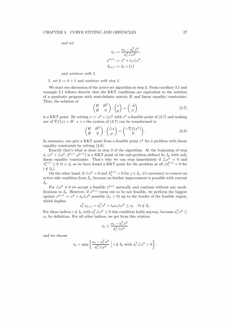
CHAPTER 3. CURVE FITTING AND OBSTACLES 27
and set
tk :=αr − aT
r xk
aTr xk
,
xk+1 := xk + tkxk,
Ik+1 := Ik ∪ r
and continue with 5.
5. set k := k + 1 and continue with step 2.
We start our discussion of the active set algorithm at step 3. From corollary 3.1 andexample 3.1 follows directly that the KKT conditions are equivalent to the solutionof a quadratic program with semi-definite matrix H and linear equality constraints.Thus, the solution of (
H BT
B 0
)·
(xµ
)=
(−bβ
)(3.7)
is a KKT point. By setting x := xk +xk with xk a feasible point of (3.7) and makinguse of ∇f(x) = H · x + c the system of (3.7) can be transformed to
(H BT
B 0
)·
(xµ
)=
(−∇f(xk)
0
). (3.8)
In summary, one gets a KKT point from a feasible point xk for a problem with linearequality constraints by solving (3.8).
Exactly that’s what is done in step 3 of the algorithm. At the beginning of step4, (xk + xk, λk+1, µk+1) is a KKT point of the sub-problem defined by Ik with onlylinear equality constraints. That’s why we can stop immediately if xk = 0 andλk+1
i ≥ 0 ∀i ∈ Ik as we have found a KKT point for the problem at all (λk+1i = 0 for
i /∈ Ik).On the other hand, if xk = 0 and λk+1
j < 0 for j ∈ Ik, it’s necessary to remove anactive side condition from Ik, because no further improvement is possible with currentIk.
For xk 6= 0 we accept a feasible xk+1 naturally and continue without any modi-fications to Ik. However, if xk+1 turns out to be not feasible, we perform the biggestupdate xk+1 := xk + tkxk possible (tk > 0) up to the border of the feasible region,which implies
aTi xk+1 = aT
i xk + tkaixk ≤ αi ∀i /∈ Ik.
For those indices i /∈ Ik with aTi xk ≤ 0 this condition holds anyway, because aT
i xk ≤αi by definition. For all other indices, we get from this relation
tk ≤αi − aT
i xk
aTi xk
and we choose
tk = min
αi − aT
i xk
aTi xk
∣∣∣ i /∈ Ik with aTi xk > 0
.

CHAPTER 3. CURVE FITTING AND OBSTACLES 28
Of course we have to add the index of the inequality side condition giving the minimumto Ik, as it is now an active inequality.
This last ”projected” update explains why the active set method belongs to theclass of projection methods in constrained optimization.
3.2 Applications
As mentioned before, curve fitting in the presence of obstacles is regarded as a con-strained non-linear optimization problem. Because of its advantageous performance,SDM is used as basic fitting algorithm and will be exposed to constraints. The penaltymethod and the active set method are applied as constrained optimization solvers.
We are going to study two different kinds of constraints. At first, the point clouditself is interpreted as obstacle. Second, the approximating curve is required to avoiduser defined smooth bounded regions in the plane.
3.2.1 Point Cloud as Obstacle
Considering the noisy point cloud in figure 2.9 for example, one might ask for anapproximation of the inner or outer border of the point cloud instead of computing afitting by means of least squared errors. This can be achieved by taking the points asobstacles into account.
Penalty Method
If we recall the description of the penalty method in algorithm 2, the penalty factorα is zero for the first number of iterations. Thus, these beginning steps are equivalentto a standard curve fitting. Only if the approximation of the point cloud is alreadysufficiently good, the penalty term is increased and starts pushing the curve out of theforbidden region.
Let the approximating B-Spline curve be oriented in such a way that the normalvector points outside. Then,
rpc(c) =∑
k∈I(c)
‖Pc(tk) − Xk‖2 (3.9)
for I(c) := i : (Pc(ti) − Xi)T· Ni < 0 defines a penalty term to approximate the
outer border of the input data points. In summary, the penalty function is
P (c, αk) =
n∑
k=0
eSDM,k(c) + λFr(c) + αk
∑
k∈I(c)
‖Pc(tk) − Xk‖2. (3.10)
Just as for the error terms in chapter 2 we need to write the penalty term asquadratic form in the displacement c. Luckily, this doesn’t require any additional workin this case because rpc(c) is the point distance minimization error term ePDM,k(c) fork ∈ I(c).

CHAPTER 3. CURVE FITTING AND OBSTACLES 29
(a) Initial setup (b) Approximation after 9 iterations withα = 0 (standard SDM)
(c) Final enclosing
αk Iterations rpc
0 9 -5 2 1.9 · 10−3
25 2 3.64 · 10−4
125 2 6.7 · 10−5
(d) Number of iterations and value of pen-alty term per penalty factor αk
Figure 3.2: Enclosing of a point cloud with the penalty method.

CHAPTER 3. CURVE FITTING AND OBSTACLES 30
Figure 3.3: Enclosing a point cloud from inside and outside with the penalty method.
Figure 3.2 shows a penalty based curve fitting enclosing the given point cloud byemploying (3.10). Factor λ of the smoothing term was set to be 0.001 in the beginningand was decreased at each iteration step. The penalty factor started at zero and wasincreased according to the rule αk+1 = 5 · αk each time the gradient of the objectivefunction was below a certain threshold of 0.3. The point cloud consists of 150 datapoints. Table 3.2d presents some key figures of the algorithm.
Figure 3.3 summarizes the result of two separate runs of the penalty based algo-rithm. The point cloud is enclosed from outside as well as from inside. Defining theorientation of the approximating B-Spline curve as before, the inner border is obtainedby replacing index set I(c) in (3.9) with I(c) := i : (Pc(ti) − Xi)
T· Ni > 0. The
smoothing term and the penalty factor didn’t change compared to the previous ex-ample, while the gradient threshold was decreased to 0.15. For each curve it took thealgorithm 15 iterations to get the final results.
Active Set Method
The active set method is the second algorithm we use to solve constrained optimizationproblems. From the discussion in section 3.1.2 we may expect results of comparablequality in a smaller number of iterations. Additionally, the active set strategy isapplicable to more scenarios as the penalty method. The latter one requires a curvealike shaped point cloud, as the first steps of the approximation are simply a standardcurve fitting. The active set method overcomes this limitation and may be used to

CHAPTER 3. CURVE FITTING AND OBSTACLES 31
(a) Initial setup (b) Final enclosing
Figure 3.4: Enclosing of a point cloud with the active set method.
enclose a point cloud representing a filled region in the plane.Defining the orientation of the approximating B-Spline curve as before,
(Pc(tk) − Xk)T· Nk > 0 0 ≤ k ≤ n
are suitable linear constraints to approximate the extent of a given set of points X =Xk : k = 0, . . . , n. Thus, the optimization problem altogether can be written as
minimize F (c) =
n∑
k=0
eSDM,k(c) + λFr(c)
subject to (Pc(tk) − Xk)T· Nk > 0 0 ≤ k ≤ n.
(3.11)
It is more convenient to rewrite these linear constraints in the form
Alc · c ≤ blc
since this was the common way restrictions were described in the theory discussedabove. Expansion of the side conditions in (3.11) and summarizing by the unknowndisplacement c gives
(Alc)i,2j...2j+1 = (−Bj(ti) · Ni)T 0 ≤ i ≤ n, 0 ≤ j ≤ m
and(blc)i = NT
i · (P (ti) − Xi) 0 ≤ i ≤ n.
In figure 3.4 the outer border of a point cloud is approximated, according to (3.11).The final enclosing was achieved after only 8 iterations of the outer general curve fittingalgorithm. The regularization factor λ was 0.0001 in the beginning and decreased ateach iteration step.
A second example may illustrate the ability of the active set method to not justreconstruct the inner and outer border of noisy curve samples but also to approximate

CHAPTER 3. CURVE FITTING AND OBSTACLES 32
(a) Initial setup (b) Final enclosing
Figure 3.5: Enclosing of a point cloud representing a filled region with the active setstrategy.
the border of a general point cloud. Figure 3.5 shows the result of this variation of aconvex hull algorithm. The smoothing factor λ was set to be 0.001 in the beginningand was reduced over the iteration.
Geometric Interpretation
Geometrically, this constrained optimization may be interpreted as follows. A mini-mization of
F (c) =
n∑
k=0
‖Pc(tk) − Xk‖2
subject to the linear inequality constraints
gk(c) = (Xk − Pc(tk))T · Nk ≤ 0 0 ≤ k ≤ n
encloses a point cloud from outside. Corollary 3.1 states that in a minimum c∗
−∇F (c∗) =∑
i∈I(c∗)
λi∇gi(c∗)
must hold. Computing the gradients and summing up gives
n∑
k=0
(Pc(tk) − Xk) =∑
i∈I(c∗)
λiNi
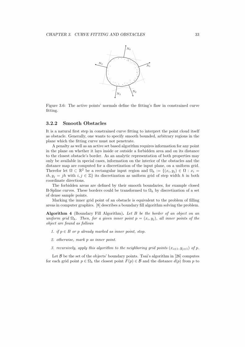
thus revealing that the overall distance of the approximating curve to the point cloudis defined as a linear combination of the curve’s normal vectors just only in the ac-tive points I(c∗). If we interpret the vectors from Xk to Pc(tk) as forces again, thedisequilibrium of the fitting is determined by the active points’ normals.
CHAPTER 3. CURVE FITTING AND OBSTACLES 33
N0
N1
N2N3
N4
Figure 3.6: The active points’ normals define the fitting’s flaw in constrained curvefitting.
3.2.2 Smooth Obstacles
It is a natural first step in constrained curve fitting to interpret the point cloud itselfas obstacle. Generally, one wants to specify smooth bounded, arbitrary regions in theplane which the fitting curve must not penetrate.
A penalty as well as an active set based algorithm requires information for any pointin the plane on whether it lays inside or outside a forbidden area and on its distanceto the closest obstacle’s border. As an analytic representation of both properties mayonly be available in special cases, information on the interior of the obstacles and thedistance map are computed for a discretization of the input plane, on a uniform grid.Therefor let Ω ⊂ R
2 be a rectangular input region and Ωh := (xi, yj) ∈ Ω : xi =ih, yj = jh with i, j ∈ Z its discretization as uniform grid of step width h in bothcoordinate directions.
The forbidden areas are defined by their smooth boundaries, for example closedB-Spline curves. These borders could be transformed to Ωh by discretization of a setof dense sample points.
Marking the inner grid point of an obstacle is equivalent to the problem of fillingareas in computer graphics. [8] describes a boundary fill algorithm solving the problem.
Algorithm 4 (Boundary Fill Algorithm). Let B be the border of an object on anuniform grid Ωh. Then, for a given inner point p = (xi, yj), all inner points of theobject are found as follows
1. if p ∈ B or p already marked as inner point, stop.
2. otherwise, mark p as inner point.
3. recursively, apply this algorithm to the neighboring grid points (xi±1, yj±1) of p.
Let B be the set of the objects’ boundary points. Tsai’s algorithm in [26] computesfor each grid point p ∈ Ωh the closest point F (p) ∈ B and the distance d(p) from p to

CHAPTER 3. CURVE FITTING AND OBSTACLES 34
F (p). This algorithm works by sweeping through Ωh. For example, sweep direction(x+, y−) means processing all points (xi, yj) ∈ Ωh in the given order j = n, . . . , 0 foreach single i = 0, . . . , n. The other sweeping directions (x+, y+), (x−, y+) and (x−, y−)are defined accordingly.
Algorithm 5 (Tsai’s Closest Point Solver). Tsai’s algorithm involves the followingsteps
1. for all discretized border points p compute the exact distance d(p) to the closestobstacle’s border and the exact foot point F (p) on that boundary. Mark theseborder grid points as done. For all other p ∈ Ω, set d(p) = ∞.
2. Iterate through each grid point p = (xi, yj) in each sweeping direction and un-dertake the following computations
(a) for each neighbor nk := (xi±1, yj±1) of p compute dtmpk = ‖p − F (nk)‖2.
(b) if dtmpk < mink d(nk), set dtmp
k = ∞.
(c) set d(p) = mink dtmpk and F (p) = F (nl) where l is the index of minimal
dtmpk .
The check on dtmpk in step 2b is necessary to ensure the monotony of the obtained
distance map d.
Penalty Method
A penalty method for curve fitting in the presence of smooth obstacles makes use ofthe information available from the two algorithms described above. The penalty termsums up the squared distances from those curve sample points inside an obstacle tothe closest obstacle’s border points
rso(c) =∑
k∈I(c)
‖Pc(tk) − Fk‖2
where I(c) := i : Pc(ti) inside an obstacle and Fk the closest point of Pc(tk) on thecorresponding obstacle’s border.
As long as there is only a single obstacle, the penalty method works straight forwardthis way by minimizing
P (c, αk) =
n∑
k=0
eSDM,k(c) + λFr(c) + αk
∑
k∈I(c)
‖Pc(tk) − Fk‖2.
However, if there are multiple obstacles, the penalty algorithm may face problems:as soon as the approximating curve leaves one forbidden region completely, it will jumpback to the interior in the next iteration step to fit the point cloud best, as there is nopenalty term for this obstacle anymore.
CHAPTER 3. CURVE FITTING AND OBSTACLES 35
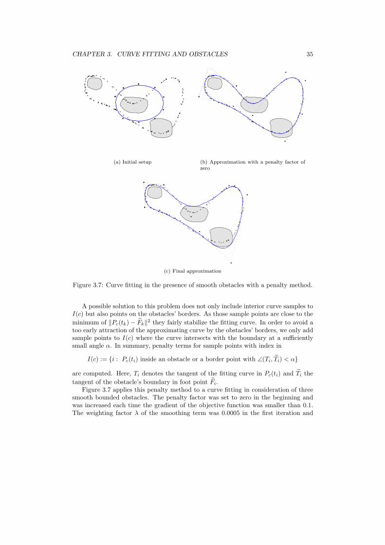
(a) Initial setup (b) Approximation with a penalty factor ofzero
(c) Final approximation
Figure 3.7: Curve fitting in the presence of smooth obstacles with a penalty method.
A possible solution to this problem does not only include interior curve samples toI(c) but also points on the obstacles’ borders. As those sample points are close to the
minimum of ‖Pc(tk) − Fk‖2 they fairly stabilize the fitting curve. In order to avoid a
too early attraction of the approximating curve by the obstacles’ borders, we only addsample points to I(c) where the curve intersects with the boundary at a sufficientlysmall angle α. In summary, penalty terms for sample points with index in
I(c) := i : Pc(ti) inside an obstacle or a border point with ∠(Ti, Ti) < α
are computed. Here, Ti denotes the tangent of the fitting curve in Pc(ti) and Ti the
tangent of the obstacle’s boundary in foot point Fi.Figure 3.7 applies this penalty method to a curve fitting in consideration of three
smooth bounded obstacles. The penalty factor was set to zero in the beginning andwas increased each time the gradient of the objective function was smaller than 0.1.The weighting factor λ of the smoothing term was 0.0005 in the first iteration and
CHAPTER 3. CURVE FITTING AND OBSTACLES 36
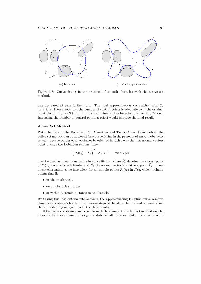
(a) Initial setup (b) Final approximation
Figure 3.8: Curve fitting in the presence of smooth obstacles with the active setmethod.
was decreased at each further turn. The final approximation was reached after 20iterations. Please note that the number of control points is adequate to fit the originalpoint cloud in figure 3.7b but not to approximate the obstacles’ borders in 3.7c well.Increasing the number of control points a priori would improve the final result.
Active Set Method
With the data of the Boundary Fill Algorithm and Tsai’s Closest Point Solver, theactive set method can be deployed for a curve fitting in the presence of smooth obstaclesas well. Let the border of all obstacles be oriented in such a way that the normal vectorspoint outside the forbidden regions. Then,
(Pc(tk) − Fk
)T
· Nk > 0 ∀k ∈ I(c)
may be used as linear constraints in curve fitting, where Fk denotes the closest pointof Pc(tk) on an obstacle border and Nk the normal vector in that foot point Fk. Theselinear constraints come into effect for all sample points Pc(tk) in I(c), which includespoints that lie
• inside an obstacle,
• on an obstacle’s border
• or within a certain distance to an obstacle.
By taking this last criteria into account, the approximating B-Spline curve remainsclose to an obstacle’s border in successive steps of the algorithm instead of penetratingthe forbidden region again to fit the data points.
If the linear constraints are active from the beginning, the active set method may beattracted by a local minimum or get unstable at all. It turned out to be advantageous
CHAPTER 3. CURVE FITTING AND OBSTACLES 37
global loop
local loop
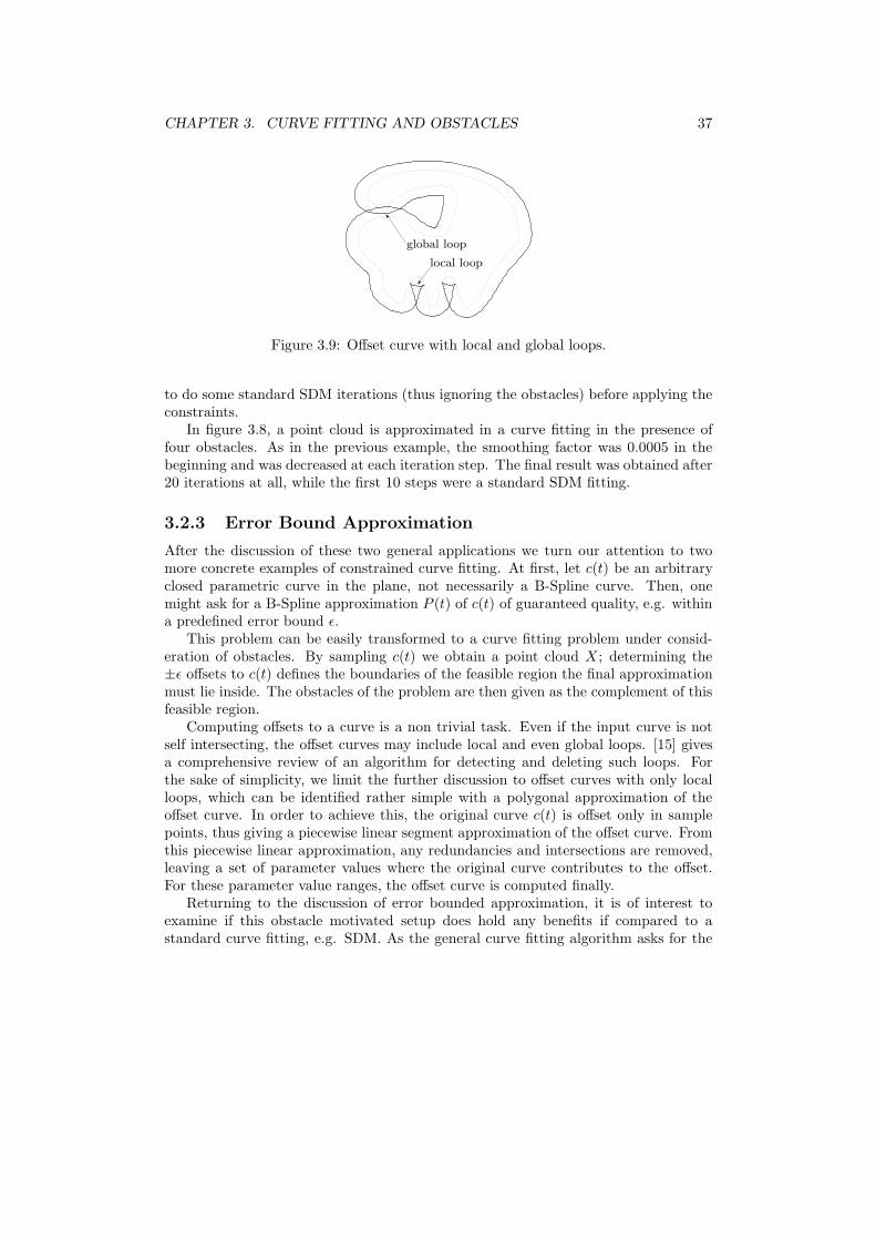
Figure 3.9: Offset curve with local and global loops.
to do some standard SDM iterations (thus ignoring the obstacles) before applying theconstraints.
In figure 3.8, a point cloud is approximated in a curve fitting in the presence offour obstacles. As in the previous example, the smoothing factor was 0.0005 in thebeginning and was decreased at each iteration step. The final result was obtained after20 iterations at all, while the first 10 steps were a standard SDM fitting.
3.2.3 Error Bound Approximation
After the discussion of these two general applications we turn our attention to twomore concrete examples of constrained curve fitting. At first, let c(t) be an arbitraryclosed parametric curve in the plane, not necessarily a B-Spline curve. Then, onemight ask for a B-Spline approximation P (t) of c(t) of guaranteed quality, e.g. withina predefined error bound ǫ.
This problem can be easily transformed to a curve fitting problem under consid-eration of obstacles. By sampling c(t) we obtain a point cloud X ; determining the±ǫ offsets to c(t) defines the boundaries of the feasible region the final approximationmust lie inside. The obstacles of the problem are then given as the complement of thisfeasible region.
Computing offsets to a curve is a non trivial task. Even if the input curve is notself intersecting, the offset curves may include local and even global loops. [15] givesa comprehensive review of an algorithm for detecting and deleting such loops. Forthe sake of simplicity, we limit the further discussion to offset curves with only localloops, which can be identified rather simple with a polygonal approximation of theoffset curve. In order to achieve this, the original curve c(t) is offset only in samplepoints, thus giving a piecewise linear segment approximation of the offset curve. Fromthis piecewise linear approximation, any redundancies and intersections are removed,leaving a set of parameter values where the original curve contributes to the offset.For these parameter value ranges, the offset curve is computed finally.
Returning to the discussion of error bounded approximation, it is of interest toexamine if this obstacle motivated setup does hold any benefits if compared to astandard curve fitting, e.g. SDM. As the general curve fitting algorithm asks for the
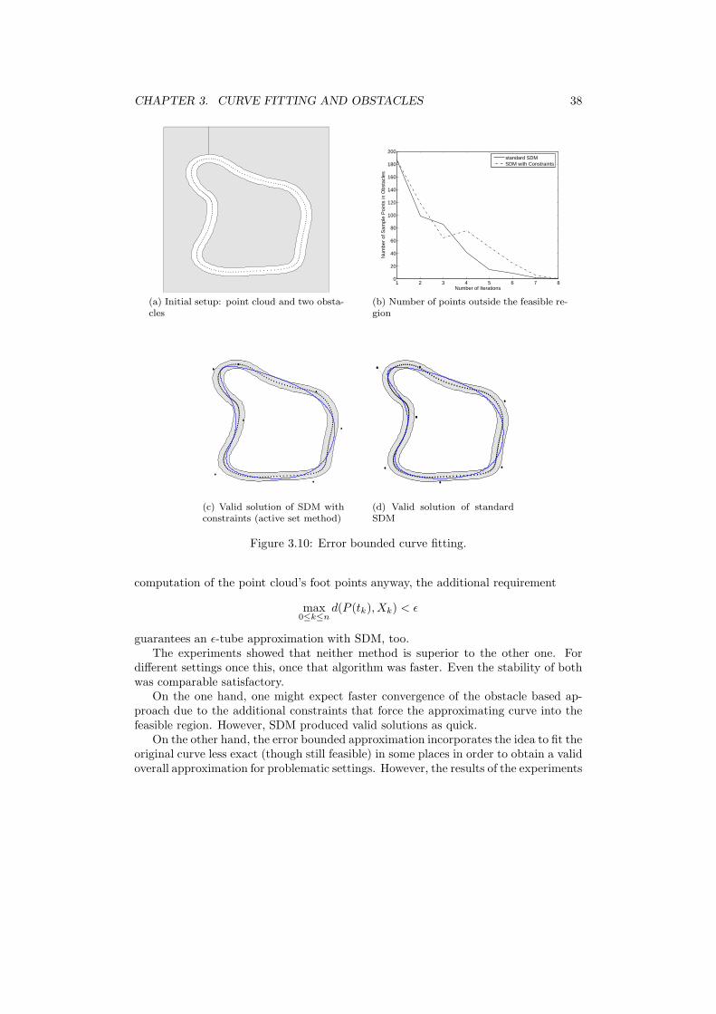
CHAPTER 3. CURVE FITTING AND OBSTACLES 38
(a) Initial setup: point cloud and two obsta-cles
1 2 3 4 5 6 7 80
20
40
60
80
100
120
140
160
180
200
Number of Iterations
Num
ber
of S
ampl
e P
oint
s in
Obs
tacl
es
standard SDMSDM with Constraints
(b) Number of points outside the feasible re-gion
(c) Valid solution of SDM withconstraints (active set method)
(d) Valid solution of standardSDM
Figure 3.10: Error bounded curve fitting.
computation of the point cloud’s foot points anyway, the additional requirement
max0≤k≤n
d(P (tk), Xk) < ǫ
guarantees an ǫ-tube approximation with SDM, too.The experiments showed that neither method is superior to the other one. For
different settings once this, once that algorithm was faster. Even the stability of bothwas comparable satisfactory.
On the one hand, one might expect faster convergence of the obstacle based ap-proach due to the additional constraints that force the approximating curve into thefeasible region. However, SDM produced valid solutions as quick.
On the other hand, the error bounded approximation incorporates the idea to fit theoriginal curve less exact (though still feasible) in some places in order to obtain a validoverall approximation for problematic settings. However, the results of the experiments

CHAPTER 3. CURVE FITTING AND OBSTACLES 39
(a) Sampled object’s boundary (b) Initial setup: point cloud after 20 shakes
(c) Final B-Spline hull after 10 iterations
Figure 3.11: B-Spline hull for a shaking object.
do not show this happening. And indeed, curve fitting with B-Splines rather requiresadditional control points in zones of bad approximation, which makes standard SDMan equivalent good solution again. The automatic insertion (and deletion) of controlpoints for SDM is discussed in [30].
Figure 3.10 compares both methods. The original curve, a B-Spline curve of degree3, was sampled to get a point cloud of 200 elements. The approximating B-Spline curvewas chosen to be of degree 2 and was ruled by seven control points. Both methodsperform similar, the resulting approximations distinguish significantly only for veryfew regions.
3.2.4 Shaking Objects
Another application of constrained curve fitting originates from the field of engineering.There, engineers face the problem of choosing an optimal hull for an object’s sweptvolume. Imagine a working engine: its shaking while in operation makes it take many

CHAPTER 3. CURVE FITTING AND OBSTACLES 40
different positions. The task is to surround the operating engine by an envelope onavoiding any contact between the engine and the hull at the same time.
Like in the previous sections we limit our discussion to the two dimensional case.The problem’s input is the boundary of the moving body, which is sampled to obtainan initial point cloud X . The shaking of the object is simulated by applying a certainnumber of random translations and rotations to the point cloud. The results of alldisplacements is summarized into a big point cloud
X :=⋃
i
αi(x) = Ri · x + ci : x ∈ X .
Matrix Ri =
(cos θi − sin θi
sin θi cos θi
)describes the two dimensional rotation matrix for
angle θi and ci ∈ R2 the i-th translation vector.
Then, computing a hull of X reduces to a curve fitting of a point cloud in thepresence of obstacles, where the obstacle is the point cloud itself (see section 3.2.1).
In figure 3.11, the computation of a B-Spline curve hull is visualized. The bound-ary of the initial object was sampled in approximately 150 points and exposed to 20movements afterward. The approximating quadratic B-Spline curve is controlled by 20control points. The final result was obtained after 10 iterations, the active set methodwas applied as constrained optimization solver.

Chapter 4
Curve Fitting on Manifolds
After studying unconstrained and constrained curve fitting of point clouds we wantto extend the work to curve fitting of point clouds on two dimensional manifolds. Inorder to avoid any approximation in three dimensions we choose the manifold to bea parametric surface and perform the optimization in the parameter space instead,while taking the inner geometry of the manifold into account at the same time. Onemight expect this additional work to improve the final fitting noticeable.
The following sections are organized as follows: first, some basic definitions andresults of Differential Geometry are sketched. Then, two modifications to the generalcurve fitting algorithm are discussed which incorporate intrinsic geometric propertiesof the manifold. Finally, experimental results of this theoretical work are presented.
4.1 Some Elementary Differential Geometry
We restrict our discussion of curve fitting on manifolds to parametrized surfaces. Incomputer aided geometric design such parametrized surfaces are very common.
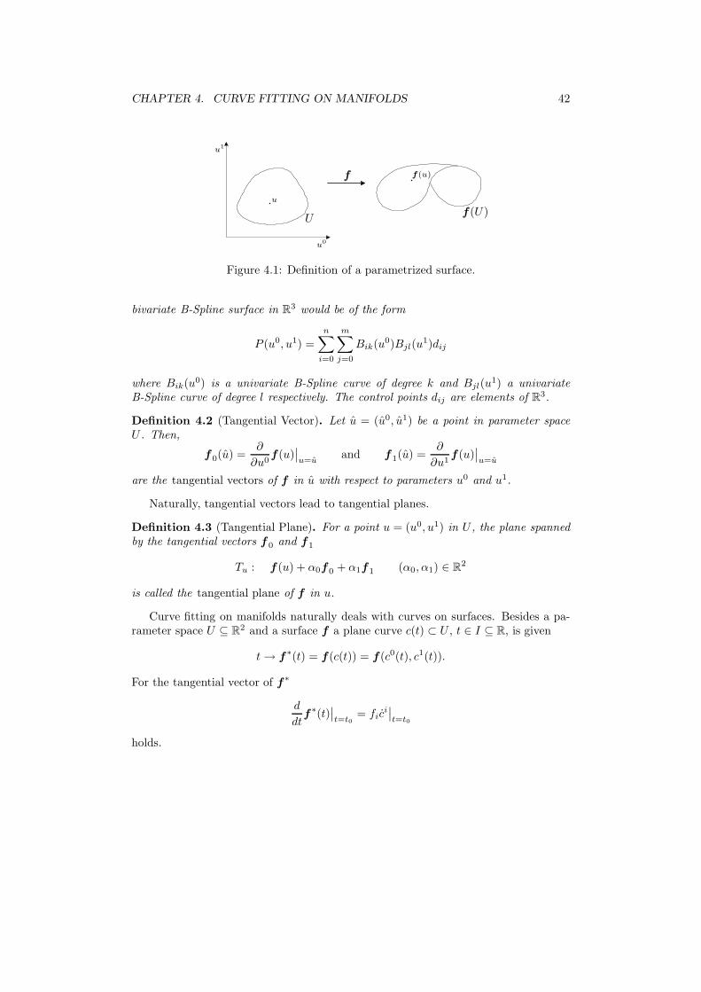
Definition 4.1 (Parametrized Surface). A parametrized surface is a vector valueddifferentiable mapping f : U ⊆ R
2 → R3. u = (u0, u1) ∈ U are called the surface’s
parameters, U is called the parameter space. f is given by its coordinate functions
f(u) =
f0(u0, u1)f1(u0, u1)f2(u0, u1)
.
B-Spline surfaces, a generalization of B-Spline curves, are a very popular examplefor parametrized surfaces.
Example 4.1 (Multivariate B-Splines). We obtain multivariate B-Splines from theunivariate B-Spline curves treated in Appendix B by a tensor product construct. A
41
CHAPTER 4. CURVE FITTING ON MANIFOLDS 42
u0
u1
u
U
f f(u)
f(U)
Figure 4.1: Definition of a parametrized surface.
bivariate B-Spline surface in R3 would be of the form
P (u0, u1) =n∑
i=0
m∑
j=0
Bik(u0)Bjl(u1)dij
where Bik(u0) is a univariate B-Spline curve of degree k and Bjl(u1) a univariate
B-Spline curve of degree l respectively. The control points dij are elements of R3.
Definition 4.2 (Tangential Vector). Let u = (u0, u1) be a point in parameter spaceU . Then,
f0(u) =∂
∂u0f(u)
∣∣u=u
and f1(u) =∂
∂u1f(u)
∣∣u=u
are the tangential vectors of f in u with respect to parameters u0 and u1.
Naturally, tangential vectors lead to tangential planes.
Definition 4.3 (Tangential Plane). For a point u = (u0, u1) in U , the plane spannedby the tangential vectors f0 and f1
Tu : f (u) + α0f0 + α1f1 (α0, α1) ∈ R2
is called the tangential plane of f in u.
Curve fitting on manifolds naturally deals with curves on surfaces. Besides a pa-rameter space U ⊆ R
2 and a surface f a plane curve c(t) ⊂ U , t ∈ I ⊆ R, is given
t → f∗(t) = f(c(t)) = f(c0(t), c1(t)).
For the tangential vector of f∗
d
dtf∗(t)
∣∣t=t0
= fici∣∣t=t0
holds.

CHAPTER 4. CURVE FITTING ON MANIFOLDS 43
PSfrag replacemen
u0
u1
c(t)
U
ff(c(t))
f(U)
c
t
I
Figure 4.2: Parametrized curve on parametrized surface.
In this expression, the Einstein summation convention comes into effect for theright handed side. According to the Einstein summation convention, an index, occur-ring more than once in a term, is summed up over all possible values. That is in thisexample
f ici∣∣t=t0
= f0c0(t0) + f1c
1(t0).
To study geometry on manifolds further, a tool to measure lengths and angles isnecessary. The first fundamental form may be used therefore.
Definition 4.4 (First Fundamental Form). The quadratic form G in a point u ∈ Udefined by
G(u) := (gij(u))i,j=1,2 =
⟨f i(u), f j(u)
⟩
is called the first fundamental form.
G(u) is a positive definite, symmetric matrix. By choosing f0(u), f1(u) as basisof the tangential plane Tu, the first fundamental form defines an Euclidean scalarproduct on Tu. In general, the first fundamental form assigns each tangential planeTu a scalar product. For two dimensional surfaces in R
3, the first fundamental formis the dot product induced from the standard scalar product in R
3 by restriction.As soon as a scalar product is available it’s possible to define a norm
‖u‖G :=√〈u, u〉G =
√uT · G(u) · u
and furthermore a metricdG(u, v) = ‖u − v‖G.
With the first fundamental form it becomes possible to work only on the surface,from an intrinsic point of view. The embedding space (the extrinsic view) isn’t impor-tant anymore.
If we consider the tangential plane Tu of f in u ∈ U again we see that it can beobtained by linearization of f in u
f (u + x) ≈ f (u) + ∇f (u)x = f(u) + f ixi.
As f0, f1 denotes a basis of Tu and f(u) is just the translation of the tangentialplane out of the origin, a point x = (x0, x1) has the same coordinates in U and in Tu.

CHAPTER 4. CURVE FITTING ON MANIFOLDS 44
Thus it’s convenient to apply the first fundamental form in the parameter space U asscalar product reflecting the inner geometry of the surface.
The first fundamental form is just a single example for a choice of a scalar productin every point of a manifold. A generalization of this concept is the Riemannian metrictensor, assigning each point of a manifold a symmetric, positive definite inner product.A manifold together with a Riemannian metric tensor is called a Riemannian manifold.
It is possible to generalize the computation of the gradient to Riemannian mani-folds. In R
n, the gradient ∇h of a continuously differentiable scalar valued function hcan be defined as that vector for which
Dvh = ∇h · v ∀v ∈ Rn (4.1)
holds, whereas Dv denotes the directional derivative of h with respect to v. Theanalogue of Dvh on surfaces is the directional derivative in a point p of the surface S
dph : Tp → R
defined by choosing v ∈ Tp and a smooth parametrized curve c : (−ǫ, ǫ) → S withc(0) = p and c(0) = v
dph(v) :=d
dt(f c)
∣∣t=0
.
By additionally replacing the standard scalar product in (4.1) with a Riemannianmetric G, we can define the gradient ∇Gh as
X = ∇Gh ⇔ dph(v) = 〈X, v〉G.
In the following, we consider only two dimensional surfaces again. In a pointp = f(u0, u1) of the surface, f0 and f1 form a basis of Tp. Thus the gradient X ∈ Tp
can be written as X = fiXi. Applying the definition of the gradient on Riemannian
manifolds and making use of the first fundamental form G as scalar product on Tp
gives∂h
∂f j
= dph(f j) = 〈X, f j〉G = 〈X if i, f j〉G = X igij .
By taking inverses, we get the components of the gradient X = ∇Gh as
X i = gij ∂h
∂f j
where gij denotes the inverse metric tensor elements. In matrix notation we can write(G symmetric!)
∇Gh = G−1∇h. (4.2)
4.2 Foot Point Computation
With the first fundamental form a measure incorporating properties of the surfaceis available for the parameter space. If we have a look at the general curve fitting
CHAPTER 4. CURVE FITTING ON MANIFOLDS 45
pg l1 l2
c(t)
d(x)=k
S
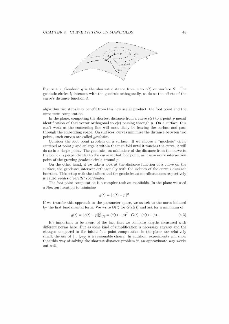
Figure 4.3: Geodesic g is the shortest distance from p to c(t) on surface S. Thegeodesic circles li intersect with the geodesic orthogonally, as do so the offsets of thecurve’s distance function d.
algorithm two steps may benefit from this new scalar product: the foot point and theerror term computation.
In the plane, computing the shortest distance from a curve c(t) to a point p meantidentification of that vector orthogonal to c(t) passing through p. On a surface, thiscan’t work as the connecting line will most likely be leaving the surface and passthrough the embedding space. On surfaces, curves minimize the distance between twopoints, such curves are called geodesics.
Consider the foot point problem on a surface. If we choose a ”geodesic” circlecentered at point p and enlarge it within the manifold until it touches the curve, it willdo so in a single point. The geodesic - as minimizer of the distance from the curve tothe point - is perpendicular to the curve in that foot point, as it is in every intersectionpoint of the growing geodesic circle around p.
On the other hand, if we take a look at the distance function of a curve on thesurface, the geodesics intersect orthogonally with the isolines of the curve’s distancefunction. This setup with the isolines and the geodesics as coordinate axes respectivelyis called geodesic parallel coordinates.
The foot point computation is a complex task on manifolds. In the plane we useda Newton iteration to minimize
g(t) = ‖c(t) − p‖2.
If we transfer this approach to the parameter space, we switch to the norm inducedby the first fundamental form. We write G(t) for G(c(t)) and ask for a minimum of
g(t) = ‖c(t) − p‖2G(t) = (c(t) − p)T · G(t) · (c(t) − p). (4.3)
It’s important to be aware of the fact that we compare lengths measured withdifferent norms here. But as some kind of simplification is necessary anyway and thechanges compared to the initial foot point computation in the plane are relativelysmall, the use of ‖ . ‖G(t) is a reasonable choice. In addition, experiments will showthat this way of solving the shortest distance problem in an approximate way worksout well.

CHAPTER 4. CURVE FITTING ON MANIFOLDS 46
Applying a Newton iteration to solve (4.3) requires the first and second derivativeof g(t). They are obtained by using the chain rule for functions in several variables
D(F G) = ((DF ) G) (DG)
where DF denotes the Jacobian
DF =
D0F0 · · · DmF0
.... . .
...D0Fn · · · DmFn
for F : Rm → R
n. DiFj means the i-th partial derivative of the j-th coordinatefunction of F .
Thus, the first derivative of (4.3) is
g′(t) = c(t) · G(t) · (c(t) − p) +1
2(c(t) − p) · G(t) · (c(t) − p)
whereas the element-wise derivation of the first fundamental form consists of terms ofthe form
d
dt
[f i(c(t)) · f j(c(t))
]= fT
i (c(t)) · Df j(c(t))c(t) + fTj (c(t)) · Df i(c(t))c(t).
Analogous, the second derivative of (4.3) turns out to be
g′′(t) = c(t) · G(t) · (c(t) − p) + 2c(t) · G(t) · (c(t) − p)+
c(t) · G(t) · c(t) +1
2(c(t) − p) · G(t) · (c(t) − p)
with the repeatedly element-wise derivated elements of G(t)
d2
dt2[f i(c(t)) · f j(c(t))
]= 2Df i(c(t)) · c(t) · Df j(c(t)) · c(t)+
fTj (c(t)) · D2f i(c(t)) · c(t) + fT
i (c(t)) · D2f j(c(t)) · c(t)+
fTj (c(t)) · Df i(c(t)) · c(t) + fT
i (c(t)) · Df j(c(t)) · c(t).
In summary, the update in the i-th step of a Newton iteration solving the footpoint problem on manifolds is given by
ti+1 = ti + δi
with
δi = −g′(ti)
g′′(ti).
By using the first fundamental form as measure for distances throughout the New-ton iteration, the successive selection rule can be applied as well for an additional stepwidth control, improving the stability of the algorithm.

CHAPTER 4. CURVE FITTING ON MANIFOLDS 47
4.3 Tangent Distance Minimization on Manifolds
Besides the foot point computation, the first fundamental form helps to adapt thegeneral curve fitting algorithm to manifolds in the computation of the error term. Instep 3 of algorithm 1, the current error of the approximation is written as a quadraticform, variable in the linear displacement of the control points. This function is thenminimized to obtain the update for the approximating B-Spline curve.
We derive a tangent distance minimization alike approximation of the squareddistance function on manifolds. Motivated by the results so far we do so in the pa-rameter space U . Let Pc(t) represent the approximating B-Spline curve, X = Xk :k = 0, . . . , n the point cloud and Pk = Pc(tk) the foot point of Xk computed withthe foot point algorithm discussed before. All these are elements of parameter spaceU . Then, a quadratic Taylor approximation of the squared distance function
d2(x) = ‖Pc(t) − x‖2
in Pk is the squared distance to the tangent in Pk
d2k(x) =
[(x − Pk)T · ∇d(Pk)
]2
(compare section 2.3.3). As d is the distance function, ‖∇d‖ = 1 holds. Expressingthis condition with the first fundamental form gives
‖∇Gd‖G =(G−1∇d
)TG · G−1∇d = ∇dT G−1∇d = 1.
Thus, we choose
esTDM,k =[(Pc(tk) − Xk)T · Nk
]2
subject to the side conditionNT
k · G−1k · Nk = 1
as error term for curve fitting on manifolds, inspired by tangent distance minimizationand realized in the parameter space.
In order to express the relation to standard TDM we refer to this method as sTDMshortly. Again, the successive reduction rule is necessary for an acceptable convergencebehavior due to the same reasons as for tangent distance minimization. The matrixnotation for TDM on surfaces does not differ from the expressions in 2.3.3 for standardTDM, with tk, dk and Nk computed as described above.
4.4 Results
The input to the following experiments are a point cloud and the approximating B-Spline curve in parameter space. In addition, we require a surface the fitting is sup-posed to happen on. Tensor product B-Spline surfaces are commonly used in CAGD.All the following surfaces are of this type, defined by 25 control points organized on a5 × 5 grid. Both univariate input B-Spline curves are of degree 2.

CHAPTER 4. CURVE FITTING ON MANIFOLDS 48
By replacing the original foot point computation with the formulas of section 4.2and using esTDM as error term, the general curve fitting algorithm 1 may be used fora curve fitting of point clouds on manifolds. Therefore, the algorithm is applied tothe curve and the point cloud in parameter space - only the final result is taken to R
3
for visualization. Like in all previous chapters, the fitting happens in two dimensions.Only this time, the surface’s properties influence the way distances are measured inU .
According to this idea, an approximation’s quality is measured with the normimplied by the first fundamental form. Thus,
eavg =1
n + 1
n∑
i=0
‖P (tk) − Xk‖2Gk
(4.4)
is used as average error, computed in parameter space.The first result is summarized in figure 4.4 and shows a curve fitting of a point
cloud with 200 points on a surface. The input situation in parameter space is given,including the approximating cubic B-Spline curve ruled by 12 control points. Similarto the standard curve fitting techniques, the smoothing term Fr2 (minimizing thebending energy) was applied. The weighting factor was set to 0.01 in the first stepand was halved at each successive iteration.
The final approximation was achieved after 20 iterations, the result is visualizedin parameter space as well as on the surface in the embedding space R
3. The dia-gram holding the decrease of the approximation error shows a reasonable convergencebehavior of sTDM.
After developing a special method for curve fitting on surfaces, the question whetherthe new algorithm outperforms a standard curve fitting neglecting any surface specificproperties arises naturally. The second experiment (in figure 4.5) compares sTDM toSDM. Of course, the initial setup was the same for both techniques and consisted of apoint cloud with 150 elements and an approximating B-Spline curve of degree 2 with9 control points.
Both methods were applied to fit the points in 30 iterations, at each step the errorwas measured with (4.4). Not only that the error of sTDM is smaller than that ofSDM, the final approximating curves are even of different shape. This advantage ofsTDM was observed throughout numerous experiments.
Chapter 3 deals with several scenarios of curve fitting in the presence of obstacles.The most general case considering smooth bounded forbidden regions can not be ap-plied directly to a fitting on surfaces, as the distance field computation would needto be adapted to take care of the surface’s characteristics. However, interpreting thepoint cloud itself as obstacle works out straight forward.
The objective function based on the sTDM error term subject to the constraints
(Pc(tk) − Xk)T· Nk > 0 0 ≤ k ≤ n
is minimized with the active set method. This is done in figure 4.6 for a point cloudconsisting of 150 points, a cubic B-Spline curve and 13 control points. The final resultwas obtained after 20 iterations.

CHAPTER 4. CURVE FITTING ON MANIFOLDS 49
(a) Initial setup in parameter space (b) Final approximation after 20 iterationsin parameter space
(c) Final approximation after 20 iterationson the surface
5 10 15 20 25 3010
−3
10−2
10−1
100
Number of Iterations
log 10
(eav
g)
(d) Decrease of error
Figure 4.4: Curve fitting on manifolds.
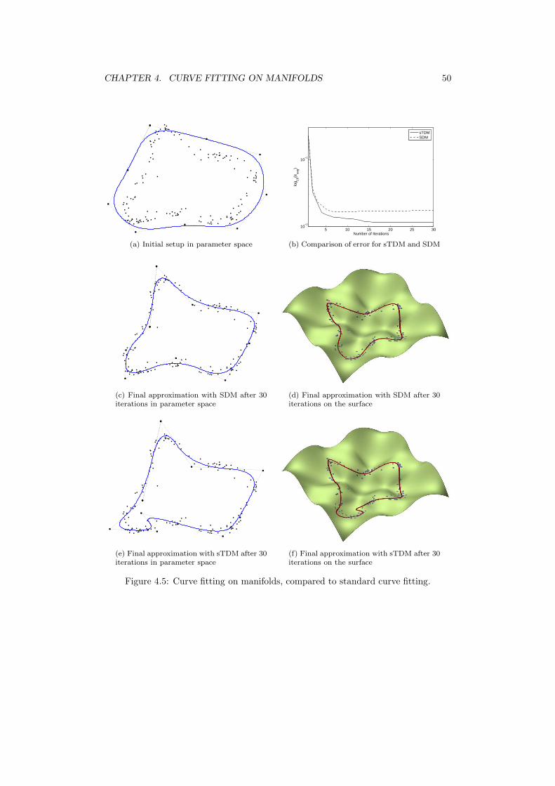
CHAPTER 4. CURVE FITTING ON MANIFOLDS 50
(a) Initial setup in parameter space
5 10 15 20 25 3010
−2
10−1
Number of Iterations
log 10
(eav
g)
sTDMSDM
(b) Comparison of error for sTDM and SDM
(c) Final approximation with SDM after 30iterations in parameter space
(d) Final approximation with SDM after 30iterations on the surface
(e) Final approximation with sTDM after 30iterations in parameter space
(f) Final approximation with sTDM after 30iterations on the surface
Figure 4.5: Curve fitting on manifolds, compared to standard curve fitting.
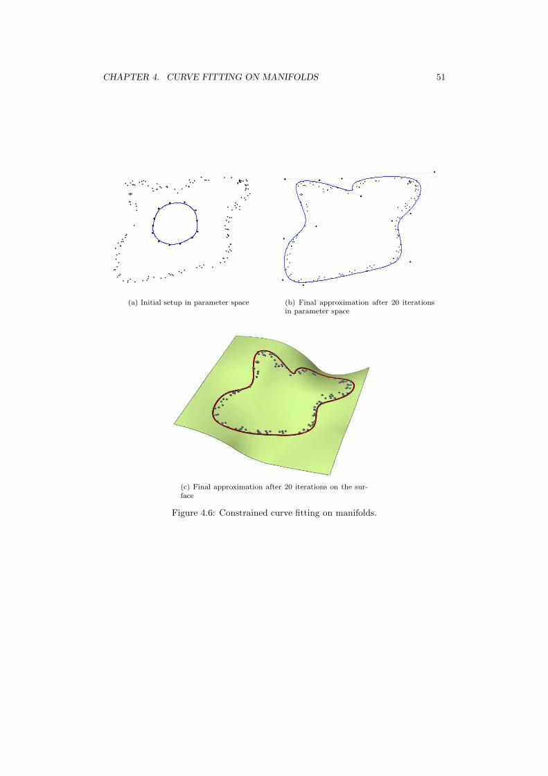
CHAPTER 4. CURVE FITTING ON MANIFOLDS 51
(a) Initial setup in parameter space (b) Final approximation after 20 iterationsin parameter space
(c) Final approximation after 20 iterations on the sur-face
Figure 4.6: Constrained curve fitting on manifolds.
Chapter 5
Curve Fitting in the L1 Norm
5.1 Introduction
So far, curve fitting relied on objective functions of the form
F (c) =
n∑
k=0
d2(Pc(tk), Xk) + λFr(c). (5.1)
A major characteristic of (5.1) is its use of the squared distance from the elements ofthe point cloud to the curve. Working with the squared distance function yields theadvantage of a straight forward to solve and easy to implement minimization problem.However, least square problems (as e.g. in the L2 norm) are known to be very sensitiveto outliers. Deploying the L1 norm instead
F (c) =
n∑
k=0
|d(Pc(tk), Xk)| + λFr(c)
promises to overcome this problem by a much more robust fitting.In the following we derive a quadratic approximation of the signed distance function
d. The basic idea is the same as in section 2.3.4, where a second order approximationof the squared distance function is formulated for SDM.
By using the same notation as in section 2.3.4, we write Pk for the foot point of theshortest distance of the approximating curve Pc(t) to the data point Xk and (Tk, Nk)for the Frenet frame in Pk. In these coordinates, Xk = (0, d) and the curvature centerK = (0, ρ). The signed distance to the circle of radius ρ centered at K turns out to be
f(x1, x2) =√
x21 + (x2 − ρ)2 − |ρ|.
Without loss of generality we may assume ρ < 0 locally. A second order Taylorapproximation of f(x1, x2) at (0, d) is thus given by
Fd(x1, x2) =1
2(d − ρ)x2
1 + x2. (5.2)
52

CHAPTER 5. CURVE FITTING IN THE L1NORM 53
x1
x2
(0,ρ)
(0,d)
Pc(t)
Fd=0
Fd>0
Fd<0
Figure 5.1: Quadratic approximation of the signed distance function.
If we compare (5.2) to the quadratic approximation (2.4) SDM is based upon, we seethat it is not only quadratic in the unknowns anymore. This is less surprising sincewe approximated the signed distance function and expect x2 (the coordinate axes indirection of Nk) to contribute its sign.
With the same argumentation as for SDM, ρ < d holds for our setup and makesthe factor of x2
1 greater than zero. The level sets of Fd are concave parabolas (in the(x1, x2) coordinate frame). Thus, Fd < 0 is true for points on the same side as thecurvature center K and Fd > 0 otherwise.
Similar to section 2.3.4 we express Fd(x1, x2) in global coordinates and get
Fd(c) =1
2(dk − ρk)
[(Pc(tk) − Xk)T · Tk
]2+ (Pc(tk) − Xk)T · Nk
where Tk and Nk are the tangent and normal in Pc(tk) respectively.In summary, curve fitting of point clouds in the L1 norm asks for a minimization
of
F (c) =n∑
k=0
el1,k(c) + λFr(c) (5.3)
where
el1,k(c) =
∣∣∣∣1
2(dk − ρk)
[(Pc(tk) − Xk)T · Tk
]2+ (Pc(tk) − Xk)T · Nk
∣∣∣∣ (5.4)
is the corresponding error term and Fr(c) a smoothing term again.We see that the general curve fitting algorithm 1 will still be applicable for curve
fitting in the L1 norm if we choose el1 as error term.Like the error terms discussed in the previous chapters we write (5.4) in matrix
notation |cT · Al1 · c + 2 · bTl1 · c + kl1|. By making use of the abbreviations
αk :=1
2(dk − ρk)
CHAPTER 5. CURVE FITTING IN THE L1NORM 54
andsk = (P (tk) − Xk)
T· Tk
we get(Al1)2i...2i+1,
2j...2j+1= αkBi(tk)Tk · T T
k Bj(tk) 0 ≤ i, j ≤ m
(bl1)2i...2i+1 = Bi(tk)(2αkskTk + Nk) 0 ≤ i ≤ m
andkl1 = αks2
k + dk.
5.2 Non-smooth Optimization
The objective function in (5.3) is a sum of absolute values. Since | . | is not differentiablefor all values we face a non-smooth optimization problem. Such problems are verycommon in practice and a wide variety of literature is available on this topic of convexoptimization. In this section we summarize some notations of non-smooth optimizationtheory and describe an algorithm to solve (5.3).
Non-smooth optimization introduces a generalization of the gradient, as the gradi-ent doesn’t exist in all cases anymore.
Definition 5.1. Let f : Rn → R be a convex function. Then, for x ∈ R
n, s ∈ Rn is
called a subgradient of f in x if
f(y) ≥ f(x) + sT (y − x) ∀y ∈ Rn.
The set of all subgradients of f in x is called the convex subdifferential ∂f(x).
If f is differentiable in x ∈ Rn and s ∈ ∂f(x), the definition of the subgradient
impliesf(x + td) − f(x) ≥ tsT d d ∈ R
n, t > 0.
Division by t and t → 0 gives
∇f(x)T d ≥ sT d ∀d ∈ Rn.
By choosing d = s −∇f(x) we get
(∇f(x) − s)T · s ≥ (∇f(x) − s)T · ∇f(x)
which is equivalent to (∇f(x) − s)2 ≤ 0. Therefore, if f is differentiable in x, thesubdifferential compromises only one element s = ∇f(x), the gradient of f in x.
Example 5.1. Let q(x) = 12xT Ax + bT x + c be a quadratic form. Then, for f(x) =
|q(x)|, the subdifferential is
∂f(x) =
Ax + b q(x) > 0α(Ax + b) − (1 − α)(Ax + b) : 0 ≤ α ≤ 1 q(x) = 0−Ax − b q(x) < 0

CHAPTER 5. CURVE FITTING IN THE L1NORM 55
Thus, a subgradient s ∈ ∂f(x) could be
s(x) =
Ax + b q(x) > 0−Ax − b q(x) ≤ 0
5.2.1 The Cutting Plane Method
Several different algorithms exist to solve non-smooth optimization problems such as(5.3). One of them is the cutting plane method.
Assume we already have a certain number of iterates x0, . . . , xk. In addition, foreach xj a subgradient sj ∈ ∂f(xj) is known. From the definition of the subgradientfollows directly
f(x) ≥ f(xj) + (sj)T (x − xj) 0 ≤ j ≤ k.
Therefore we can write
f(x) ≥ max0≤j≤k
f(xj) + (sj)T (x − xj)
=: fk(x).
fk(x) is a piecewise linear lower bound approximation of f(x). The basic idea of
the cutting plane method is to get the next iterate xk+1 by minimizing fk(x). As fk(x)is expected to approximate f(x) better for increasing k, the solution of
min fk(x) (5.5)
should approach a solution of the original non-smooth optimization problem for suffi-cient large k.
Lemma 5.1. xk+1 solves (5.5) if and only if (xk+1, ζk+1) ∈ Rn × R with ζk+1 :=
fk(xk+1) is a solution of
minimize ζsubject to f(xj) + (sj)T (x − xj) ≤ ζ 0 ≤ j ≤ k.
(5.6)
Proof. At first, let xk+1 be a solution of (5.5) and assume (xk+1, ζk+1) is not optimalfor (5.6). Then, there exists a (x, ζ) with ζ < ζk+1. Thus,
fk(x) = ζ < ζk+1 = fk(xk+1)
which is a contradiction to xk+1 being the optimal solution of (5.5).On the other hand, if (xk+1, ζk+1) is the optimal solution of (5.6), we assume that
xk+1 doesn’t solve (5.5). So there exists a x with ζ = fk(x) < fk(xk+1). From this itfollows that
ζ = fk(x) < fk(xk+1) = ζk+1
which is again a contradiction to (xk+1, ζk+1) being the optimal solution of (5.6).
CHAPTER 5. CURVE FITTING IN THE L1NORM 56
By making use of the previous lemma we are able to transform the non-smoothoptimization problem (5.5) to a smooth, constrained, linear program. The linearconstraints in (5.6) cut off regions of the solution space, thus giving the method itsname.
For application it turned out to be crucial to generalize (5.6) by adding a regular-ization term (”proximal term”)
minimize ζ + µk‖x − xk‖2
subject to f(xj) + (sj)T (x − xj) ≤ ζ 0 ≤ j ≤ k(5.7)
where µk denotes a monotone decreasing coefficient.(5.7) is a quadratic optimization problem with linear constraints that can be solved
by any standard technique such as the active set method. The structure of the mini-mization problem allows us to add additional constraints to restrict the solution spaceof x further.
Our common way to describe minimization problems is to write the objective func-tion as quadratic form and any constraints as system of linear inequalities. For (5.7)this gives for c = ( c
ζ ) with c ∈ R2m+2, ζ ∈ R, and I =
(I2m+2 0
0 0
)∈ R
2m+3 × R2m+3
minimize 12 · cT · I · c −
(ck
−1
)T
· c + 12
(ck
0
)T
· I ·
(ck
0
)
subject to
(sj
−1
)T
· c ≤ (sj)T · cj − f(cj) 0 ≤ j ≤ k.
Al1, bl1 and kl1 influence the problem only in the computation of sj and f(cj) =(cj)T · Al1 · c
j + 2 · bTl1 · c
j + kl1.
Algorithm 6 (Cutting Plane). Finally, a cutting plane algorithm involves the follow-ing steps
1. choose x0, set k = 0.
2. if xk is a reasonable good approximation of a minimum, leave.
3. otherwise, compute sk ∈ ∂f(xk).
4. solve the corresponding constrained quadratic program (5.7).
5. increase k and continue with step 2.
The following lemma gives a suitable stopping criteria for step 2.
Lemma 5.2. Let the non-smooth optimization problem min f(x) have a solution x∗.Furthermore xk describes the sequence of iterates obtained by the cutting plane
method and we write ζk+1 = fk(xk+1) again. If
f(xk+1) − ζk+1 ≤ ǫ
for ǫ > 0, thenf(xk+1) − f∗ ≤ ǫ
holds, whereas f∗ := f(x∗).
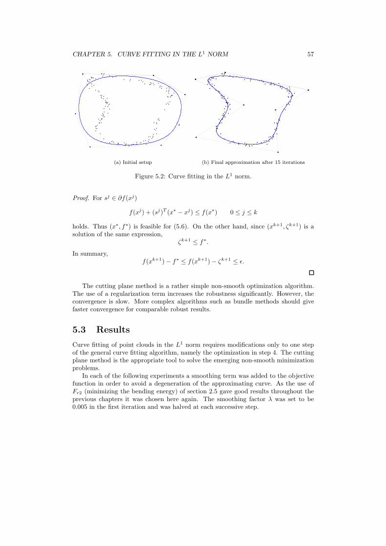
CHAPTER 5. CURVE FITTING IN THE L1NORM 57
(a) Initial setup (b) Final approximation after 15 iterations
Figure 5.2: Curve fitting in the L1 norm.
Proof. For sj ∈ ∂f(xj)
f(xj) + (sj)T (x∗ − xj) ≤ f(x∗) 0 ≤ j ≤ k
holds. Thus (x∗, f∗) is feasible for (5.6). On the other hand, since (xk+1, ζk+1) is asolution of the same expression,
ζk+1 ≤ f∗.
In summary,f(xk+1) − f∗ ≤ f(xk+1) − ζk+1 ≤ ǫ.
The cutting plane method is a rather simple non-smooth optimization algorithm.The use of a regularization term increases the robustness significantly. However, theconvergence is slow. More complex algorithms such as bundle methods should givefaster convergence for comparable robust results.
5.3 Results
Curve fitting of point clouds in the L1 norm requires modifications only to one stepof the general curve fitting algorithm, namely the optimization in step 4. The cuttingplane method is the appropriate tool to solve the emerging non-smooth minimizationproblems.
In each of the following experiments a smoothing term was added to the objectivefunction in order to avoid a degeneration of the approximating curve. As the use ofFr2 (minimizing the bending energy) of section 2.5 gave good results throughout theprevious chapters it was chosen here again. The smoothing factor λ was set to be0.005 in the first iteration and was halved at each successive step.

CHAPTER 5. CURVE FITTING IN THE L1NORM 58
5 10 15 20 25 30
10−2
10−1
Number of Iterationslo
g 10(e
avg)
Figure 5.3: Decrease of error for the L1 fitting in figure 5.2.
As mentioned in the theoretical presentation of the cutting plane method, thegeneralized form of (5.7) makes the optimization much more robust. The coefficient ofthe regulating term ‖x − xk‖2 was set to µk = e10−k, where k stands for the currentiteration.
Lemma 5.2 gives a possible stopping criteria for the cutting plane method. Wemade use of it and set ǫ = 10−4. It’s worth mentioning that single calls to the non-smooth minimization routine with these parameters took up to 200 iterations in theworst case to find a solution.
The first result of a curve fitting in L1 norm in figure 5.2 is a simple proof ofconcept for the method described above. The point cloud consisted of 150 points andwas approximated with a cubic B-Spline controlled by 8 de Boor-points. The finalapproximation was obtained after 15 iterations of the general curve fitting algorithm.
In difference to the curve fitting methods of the preceding sections we employ adifferent error measure here. Naturally, we replace the squared distance by absolutevalues, thus using the average sum of residues
eavg =1
n + 1
n∑
k=0
|P (tk) − Xk|.
Figure 5.3 visualizes the decrease of the average approximating error for the experimentof figure 5.2.
The development of a curve fitting in the L1 norm was motivated by the well knownfact that the L2 norm is very sensitive to outliers. The second experiment focuses onthis issue by adding four significant outliers to a point cloud with 150 elements. Theapproximating B-Spline curve was of degree 3 and had 8 control points.
The results of this second experiment are illustrated in figure 5.4. While the so-lution obtained with the squared distance minimization algorithm is attracted clearlyby the four additional points, the L1 based approach is not influenced visually. Twoadditional diagrams show the development of the average absolute error as well as theaverage distance error. As expected, SDM minimizes the squared distance better whilethe approximation in the L1 norm gives a smaller average absolute error.

CHAPTER 5. CURVE FITTING IN THE L1NORM 59
(a) Final approximation with SDM after 30iterations
(b) Final approximation in L1 norm after 30iterations
5 10 15 20 25 30
10−3
10−2
Number of Iterations
Ave
rage
squ
ared
dis
tanc
e er
ror
L1 approximationSDM
(c) Comparison of both methods’average distance error
5 10 15 20 25 30
10−2
10−1
Number of Iterations
Ave
rage
abs
olut
e er
ror
L1 approximationSDM
(d) Comparison of both methods’average absolute error
Figure 5.4: Comparison of curve fitting with SDM and in the L1 norm.
Figure 5.5: Constrained non-smooth optimization to enclose a point cloud.
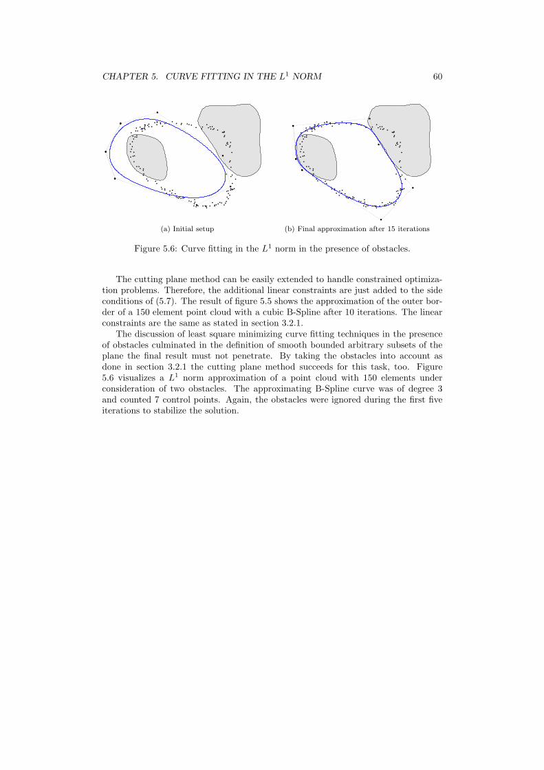
CHAPTER 5. CURVE FITTING IN THE L1NORM 60
(a) Initial setup (b) Final approximation after 15 iterations
Figure 5.6: Curve fitting in the L1 norm in the presence of obstacles.
The cutting plane method can be easily extended to handle constrained optimiza-tion problems. Therefore, the additional linear constraints are just added to the sideconditions of (5.7). The result of figure 5.5 shows the approximation of the outer bor-der of a 150 element point cloud with a cubic B-Spline after 10 iterations. The linearconstraints are the same as stated in section 3.2.1.
The discussion of least square minimizing curve fitting techniques in the presenceof obstacles culminated in the definition of smooth bounded arbitrary subsets of theplane the final result must not penetrate. By taking the obstacles into account asdone in section 3.2.1 the cutting plane method succeeds for this task, too. Figure5.6 visualizes a L1 norm approximation of a point cloud with 150 elements underconsideration of two obstacles. The approximating B-Spline curve was of degree 3and counted 7 control points. Again, the obstacles were ignored during the first fiveiterations to stabilize the solution.

Bibliography
[1] Christian Bar. Elementare Differentialgeometrie. de Gruyter, 2001.
[2] Pal Benk, Geza Kos, Tamas Varady, Laszlo Andor and Ralph Martin. Constrainedfitting in reverse engineering. Computer Aided Geomtric Design, Vol. 19, 3:173-205, 2002.
[3] Andrew Blake and Michael Isard. Active Contours. Springer, London, 2nd edition,2000.
[4] Martin Brokate. Praktische Analysis. Volesungsskript Universitat Kiel, 1998.
[5] Carsten Carstensen. Numerische Mathematik II. Volesungsskript TU Wien, 2003.
[6] Carl Geiger and Christian Kanzow. Theorie und Numerik restringierter Opti-mierungsaufgaben. Springer, 2002.
[7] Yaroslav Halchenko. Iterative closest point algorithm. L1 error approach via linearprogramming. Report, New Jersey Institute of Technology, 2003.
[8] Donald Hearn and M. Pauline Baker. Computer Graphics. Prentice Hall, 1997.
[9] Jean-Baptiste Hiriart-Urruty, Claude Lemarechal. Convex analysis and minimiza-tion algorithms. Springer, 1998.
[10] Michael Hofer and Helmut Pottmann. Energy-Minimizing Splines in Manifolds.ACM Transactions on Graphics (Proceedings of ACM SIGGRAPH), Vol. 23,3:284-293, 2004.
[11] Josef Hoschek. Intrinsic parameterization for approximation. Computer AidedGeomtric Design, 5:27-31, 1988.
[12] Bert Juttler. Differentialgeometrie. Vorlesungsskript Johannes Kepler UniversitatLinz, Sommersemester 2005.
[13] C.T. Kelley. Iterative methods for optimization. SIAM: Frontiers in Applied Math-ematics 18, 1999.
[14] Wolfgang Kuhnel. Differentialgeometrie. Vieweg, 2003.
61

BIBLIOGRAPHY 62
[15] In-Kwon Lee, Myung-Soo Kim and Gershon Elber. Planar curve offset based oncircle approximation. Computer-Aided Design, Vol. 28, 8:617-630; 1996.
[16] Marko M. Makela and Pekka Neittaamaki. Nonsmooth Optimization. World Sci-entific Publishing, 1992.
[17] Ashish Myles and Jorg Peters. Threading splines through 3D channels. Computer-Aided Design, Vol. 37, pages 139-148, 2005.
[18] Jorg Peters and Xiaobin Wu. SLEVEs for planar spline curves. Computer AidedGeometric Design, Vol. 21, 6:615-635, 2004.
[19] Les Piegl and Wayne Tiller. The NURBS book. Springer, Berlin, 1995.
[20] Michael Plass and Maureen Stone. Curve-fitting with piecewise parametric cubics.Computer Graphics, Vol. 17, 3:229-239, 1983.
[21] Helmut Pottmann and Michael Hofer. Geometry of the Squared Distance Functionto Curves and Surfaces. In H.C. Hege and K. Polthiers, editors, Visualization andMathematics III, pages 223-244, 2003.
[22] Helmut Pottmann and Stefan Leopoldseder. A concept for parametric surfacefitting which avoids the parametrization problem. Computer Aided Geometric De-sign, Vol. 20, 6:343-362, 2003.
[23] Helmut Pottmann, Stefan Leopoldseder and Michael Hofer. Approximation withactive B-spline curves and surfaces. Proceedings of Pacific Graphics 2002, pages8-25. IEEE Computer Society Press, 2002.
[24] Gabor Renner and Volker Weiß. Exact and approximate computation of B-splinecurves on surfaces. Computer-Aided Design, Vol. 36, 4:351-362, 2004.
[25] Eric Saux, Marc Daniel. An improved Hoschek intrinsic parametrization. Com-puter Aided Geomtric Design, 20:513-521, 2003.
[26] Yen-hsi Richard Tsai. Rapid and Accurate Computation of the Distance FunctionUsing Grids. Journal of Computational Physics 178:175-195, 2002.
[27] Johannes Wallner and Qinmin Yang. Swept volumes of many poses. In M. Des-brun and H. Pottmann, editors, SGP 2005: Third Eurographics Symposium onGeometry processing, pages 161-170. Eurographics Association, 2005.
[28] Wenping Wang, Helmut Pottmann, Yang Liu. Fitting B-Spline Curves to PointClouds by Squared Distance Minimization. Preprint, University of Hong Kong,2004.
[29] Volker Weiss, Laszl Andor, Gabor Renner and Tamas Varady. Advanced surfacefitting techniques. Computer Aided Geometric Design, 19:19-42, 2002.
[30] Huaiping Yang, Wenping Wang and Jiaguang Sunb. Control point adjustment forB-spline curve approximation. Computer-Aided Design, Vol. 36, pages 639-652,2004.
Appendix A
Splines
Curve design and interpolation problems are important topics in Geometry and Nu-merical Mathematics. Polynomial based approaches serve well due to their simpleformulation and their easy implementation in computer software. However, lookingfor a single polynomial meeting certain criteria (e.g. a certain number of interpolatingpoints) soon leads to functions of high polynomial degree. As this is neither intendednor useful in most cases, splines - piecewise polynomial functions - represent a moreconvenient solution to such problems.
Definition A.1 (Spline). Let ∆n : a = x0 < x1 < . . . < xn = b be a partition of[a, b] ∈ R. Then, s : [a, b] → R is called a (polynomial) spline of degree m for partition∆n if
s ∈ Cm−1[a, b] (A.1)
s|[xj,xj+1] ∈ Pm = p : deg(p) ≤ m 0 ≤ j < n (A.2)
The set of all s meeting (A.1) and (A.2) is denoted by Sm(∆n).
S1(∆n), S2(∆n) and S3(∆n) are called linear, quadratic and cubic splines.
Theorem A.1. Sm(∆n) is a vector space of dimension m + n. A basis of Sm(∆n) isgiven by B = p0, . . . , pm, q1, . . . , qn−1 with
pi(x) = (x − x0)i 0 ≤ i ≤ m
qj(x) = (x − xj)m+ =
(x − xj)
m x ≥ xj
0 thus1 ≤ j < n
Proof. B ⊂ Sm(∆n) is obvious due to construction. In order to prove the linearindependence of B, let
s(x) =
m∑
i=0
αipi(x) +
n−1∑
j=1
βjqj(x) ∀x ∈ [a, b].
63

APPENDIX A. SPLINES 64
On [x0, x1] we have
0 = s(x) =
m∑
i=0
αipi(x)
whereas follows αi = 0 for 0 ≤ i ≤ m, as the pi are linearly independent. On [x1, x2],s(x) simplifies to 0 = s(x) = β1q1(x), therefore β1 = 0. Analogous β2, . . . , βn−1 = 0 isshown and gives the linear independence of B.
B is a spanning set of Sm(∆n): As s|[x0,x1] ∈ Pm there exists a z1 ∈ Pm withz1|[x0,x1] = s|[x0,x1] and z1 ∈ spanp0, . . . , pm. For j = 2, . . . , n we define
zj(x) = zj−1(x) + νj−1qj−1(x) with zj(xj) = s(xj).
Then, the difference r := s − zn ∈ Sm(∆n), as in general
zj ∈ spanp0, . . . , pm, q1, . . . , qj−1.
On [x0, x1], r = z1 − zn ∈ spanq1, . . . , qn−1 and therefore r|[x0,x1] ≡ 0. On [x1, x2], rpossesses a m-fold zero at x1 (r ∈ Cm−1[a, b]) and at x2 r = s−zn = s−z2 a single zero.Thus, r ≡ 0 on [x1, x2]. By applying this argumentation to [x2, x3], . . . , [xn−1, xn] weget r ≡ 0 on [a, b].
Unfortunately, this basis turns out to be rather useless for application as its numeri-cal characteristics are poor: if elements of Sm(∆n) are written as linear combination ofB, the coefficients tend to grow large. B-Splines define a numerical more advantageousbasis of Sm(∆n).
Definition A.2 (B-Spline). Let (ti)i∈Z ∈ R : . . . ≤ t−2 ≤ t−1 ≤ t0 ≤ t1 ≤ t2 ≤ . . .be a monotone increasing sequence (called knot sequence). Then, the B-Spline Bik ofdegree k for knot sequence (ti)i∈Z is recursively defined by
Bi0(x) =
1 ti ≤ x < ti+1
0 thusBik(x) = wik(x)Bi,k−1(x) + (1 − wi+1,k(x))Bi+1,k−1(x)
The coefficients wik(x) are given by
wik(x) =
x−ti
ti+k−titi < ti+k
0 ti = ti+k
Some important properties of B-Splines are summarized in the following lemma.
Lemma A.1. Let Bik be a B-Spline for a given knot sequence (ti)i∈Z. Then, thefollowing properties hold
Bik|[tj ,tj+1) ∈ Pk (A.3)
supp(Bik) = x : Bik(x) 6= 0 = [ti, ti+k+1] ti < ti+k+1 (A.4)
Bik = 0 ti = ti+k+1 (A.5)
APPENDIX A. SPLINES 65
Bik ≥ 0 (A.6)∑
i∈Z
Bik = 1 (A.7)
Proof. Propositions (A.3) to (A.6) follow directly from the B-Spline definition. (A.7)is shown by induction over k. The initial case k = 0 is trivial. For k − 1 → k:
∑
i∈Z
Bik =∑
i∈Z
wi,kBi,k−1 + (1 − wi+1,k)Bi+1,k−1
=∑
i∈Z
wi,kBi,k−1 +∑
i∈Z
Bi+1,k−1 −∑
i∈Z
wi+1,kBi+1,k−1
=∑
i∈Z
Bi+1,k−1 =∑
i∈Z
Bi,k−1 = 1
The proof of the basis property of B-Splines for Sm(∆n) makes use of Marsden’sIdentity.
Lemma A.2 (Marsden’s Identity). Let Bik describe the B-Splines for a given knotsequence (ti)i∈Z. Then
(x − ζ)k =∑
i∈Z
φik(ζ)Bik(x)
with φi0(ζ) = 1, φik(ζ) =
k∏
l=1
(ti+l − ζ).
Proof. Marsden’s Identity is proved by induction over k. k = 0 is obvious due to (A.7).For k − 1 → k we apply the recursive definition of B-Splines
∑
i∈Z
φik(ζ)Bik(x) =∑
i∈Z
φik(ζ) [wik(x)Bi,k−1(x) + (1 − wi+1,k(x))Bi+1,k−1(x)]
=∑
i∈Z
[φik(ζ)wik(x) + φi−1,k(ζ)(1 − wik(x))] Bi,k−1(x)
For fixed i ∈ Z we simplify the coefficient of Bi,k−1(x):
φik(ζ)wik(x) + φi−1,k(ζ)(1 − wik(x)) = φik(ζ)x − ti
ti+k − ti+ φi−1,k(ζ)
ti+k − x
ti+k − ti
= (x − ζ)φik(ζ) − φi−1,k(ζ)
ti+k − ti+
φik(ζ)(ζ − ti) + φi−1,k(ζ)(ti+k − ζ)
ti+k − ti
= (x − ζ)[(ti+k − ζ) − (ti − ζ)] φi,k−1(ζ)
ti+k − ti= (x − ζ)φi,k−1(ζ).
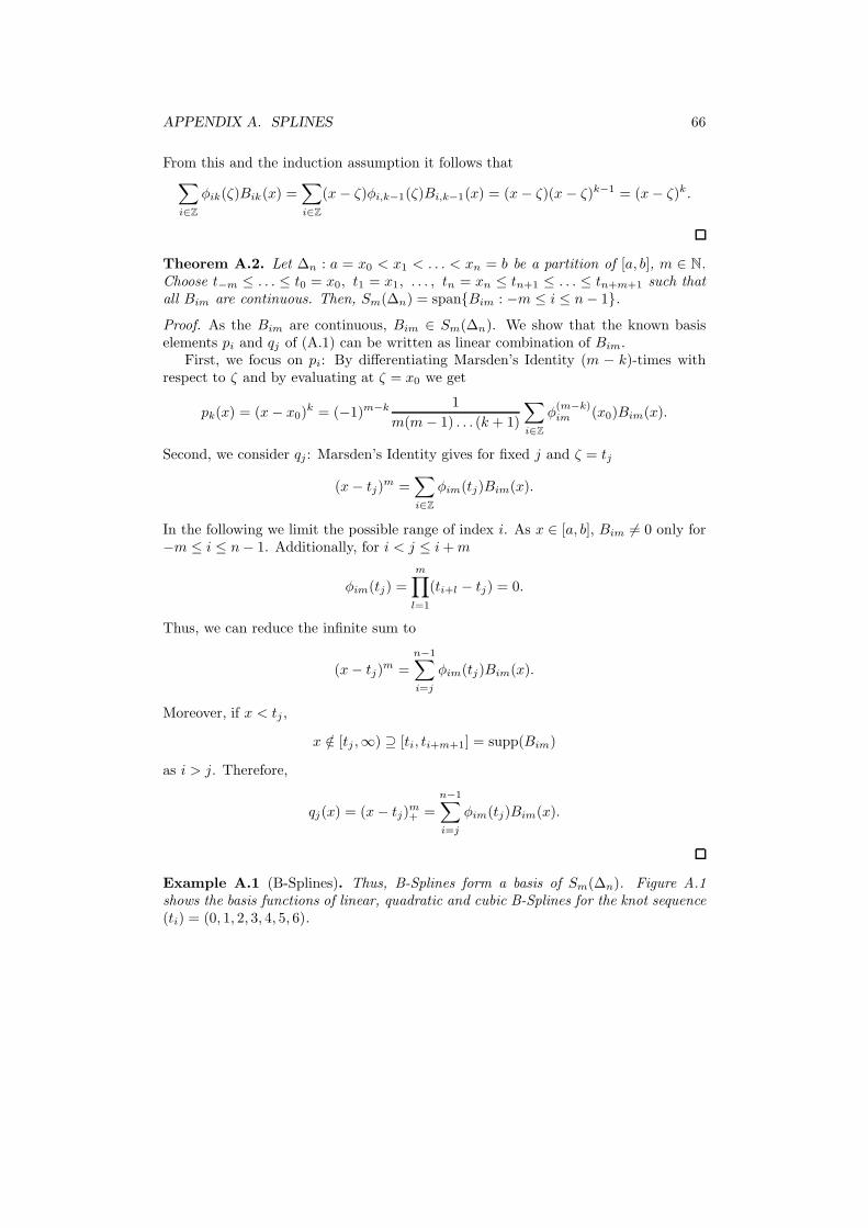
APPENDIX A. SPLINES 66
From this and the induction assumption it follows that∑
i∈Z
φik(ζ)Bik(x) =∑
i∈Z
(x − ζ)φi,k−1(ζ)Bi,k−1(x) = (x − ζ)(x − ζ)k−1 = (x − ζ)k.
Theorem A.2. Let ∆n : a = x0 < x1 < . . . < xn = b be a partition of [a, b], m ∈ N.Choose t−m ≤ . . . ≤ t0 = x0, t1 = x1, . . . , tn = xn ≤ tn+1 ≤ . . . ≤ tn+m+1 such thatall Bim are continuous. Then, Sm(∆n) = spanBim : −m ≤ i ≤ n − 1.
Proof. As the Bim are continuous, Bim ∈ Sm(∆n). We show that the known basiselements pi and qj of (A.1) can be written as linear combination of Bim.
First, we focus on pi: By differentiating Marsden’s Identity (m − k)-times withrespect to ζ and by evaluating at ζ = x0 we get
pk(x) = (x − x0)k = (−1)m−k 1
m(m − 1) . . . (k + 1)
∑
i∈Z
φ(m−k)im (x0)Bim(x).
Second, we consider qj : Marsden’s Identity gives for fixed j and ζ = tj
(x − tj)m =
∑
i∈Z
φim(tj)Bim(x).
In the following we limit the possible range of index i. As x ∈ [a, b], Bim 6= 0 only for−m ≤ i ≤ n − 1. Additionally, for i < j ≤ i + m
φim(tj) =
m∏
l=1
(ti+l − tj) = 0.
Thus, we can reduce the infinite sum to
(x − tj)m =
n−1∑
i=j
φim(tj)Bim(x).
Moreover, if x < tj ,
x /∈ [tj ,∞) ⊇ [ti, ti+m+1] = supp(Bim)
as i > j. Therefore,
qj(x) = (x − tj)m+ =
n−1∑
i=j
φim(tj)Bim(x).
Example A.1 (B-Splines). Thus, B-Splines form a basis of Sm(∆n). Figure A.1shows the basis functions of linear, quadratic and cubic B-Splines for the knot sequence(ti) = (0, 1, 2, 3, 4, 5, 6).
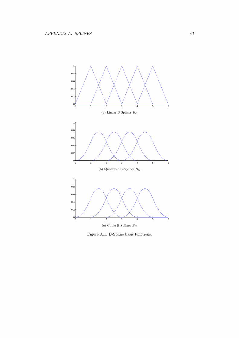
APPENDIX A. SPLINES 67
0 1 2 3 4 5 60
0.2
0.4
0.6
0.8
1
(a) Linear B-Splines Bi1
0 1 2 3 4 5 60
0.2
0.4
0.6
0.8
1
(b) Quadratic B-Splines Bi2
0 1 2 3 4 5 60
0.2
0.4
0.6
0.8
1
(c) Cubic B-Splines Bi3
Figure A.1: B-Spline basis functions.
Appendix B
B-Spline Curves
With B-Splines we have an advantageous basis of Sm(∆n), the vector space of allsplines of degree m for a given partition ∆n. In a next step, these basis elements arecombined to form B-Spline curves. In computer aided geometric design it’s desirableto control the design of curves or surfaces with parameters, which ideally can be linkeddirectly to the geometry of the created objects. For B-Spline curves the coefficientsof linear combinations of the basis B-Splines, often called control points, will play thisrole.
Definition B.1 (B-Spline Curve). Let (ti)i∈Z be a knot sequence and Bik the corre-sponding B-Splines. Furthermore, (di)i∈Z ∈ R
d is a sequence of given control points.Then, P : R → R
d
P (t) =∑
i∈Z
Bik(t)di
is called B-Spline Curve of degree k. The control points di are called de Boor-points,too.
The general properties of B-Splines of lemma A.1 naturally have a bearing on B-Spline curves. If the curve parameter t originates from [ti, ti+k+1], Bik = 0 holds fori < 0 and i > n due to (A.3). Therefore, the B-Spline curve can be written as finitesum
P (t) =
n∑
i=0
Bik(t)di.
As another conclusion from this lemma a control point di influences the curve P (t)only on [ti, ti+k+1]. Additionally, under these assumptions,
∑ni=0 Bik(t) = 1 holds.
Thus, the B-Spline curve P (t) is in the convex hull of the control points di.
Example B.1 (Open B-Spline Curve). For the given control points
(0.07
0.57
),
(0.25
0.81
),
(0.37
0.45
),
(0.35
0.27
),
(0.60
0.37
),
(0.59
0.60
),
(0.85
0.69
)
68

APPENDIX B. B-SPLINE CURVES 69
Figure B.1: Open B-Spline Curve.
we want to create a B-Spline curve of degree 3, interpolating the first and last controlpoint respectively. The corresponding knot sequence is for example
(0, 0, 0, 0, 0.25, 0.5, 0.75, 1, 1, 1, 1).
The B-Spline curve is given by
P (t) =
6∑
i=0
Bi3(t)di t ∈ [0, 1]
the result is plotted in figure B.1.
Example B.2 (Closed B-Spline Curve). In order to create the quadratic closed B-Spline Curve of figure B.2 for the control points
(0.2
0.62
),
(0.44
0.83
),
(0.72
0.61
),
(0.69
0.35
),
(0.48
0.34
),
(0.41
0.57
),
(0.18
0.50
)
the knot sequence can be chosen as(− 2
7 , − 17 , 0, 1
7 , 27 , 3
7 , 47 , 5
7 , 67 , 1, 8
7 , 97
).
The first two control points need to be repeated
d0, d1, . . . , d6, d7 = d0, d8 = d1.
Then, the closed B-Spline curve of degree 2 is
P (t) =
8∑
i=0
Bi2(t)di t ∈ [0, 1].

APPENDIX B. B-SPLINE CURVES 70
Figure B.2: Closed B-Spline Curve.