High Accuracy Terrain Reconstructionfrom Point Clouds Using Implicit

Deformable Model

Jules Morel1(B) , Alexandra Bac2 , and Takashi Kanai1

1 Kanai Laboratory, Graduate School of Arts and Sciences,The University of Tokyo, Tokyo, Japan

jules.morel@ifpindia.org2 Laboratoire d’Informatique et des Systemes, Aix Marseille University,

Marseille, France

Abstract. Few previous works have studied the modeling of forestground surfaces from LiDAR point clouds using implicit functions. [10] isa pioneer in this area. However, by design this approach proposes over-smoothed surfaces, in particular in highly occluded areas, limiting itsability to reconstruct fine-grained terrain surfaces. This paper presentsa method designed to finely approximate ground surfaces by relying ondeep learning to separate vegetation from potential ground points, fillingholes by blending multiple local approximations through the partition ofunity principle, then improving the accuracy of the reconstructed sur-faces by pushing the surface towards the data points through an iterativeconvection model.

Keywords: Implicit surface · Deformable model · Deep learning

1 Introduction

Digital terrain model (DTM) extraction is an important issue in the field ofLiDAR remote sensing of Earth surface. Indeed, further data processing proce-dures (segmentation, surface reconstruction, digital volume computation) usu-ally rely on a prior DTM computation to focus on features of interest (buildings,roads or trees for instance). In the last two decades, many filtering algorithmshave been proposed to solve this problem using Airborne LiDAR sensors (ALS)data.

However, most previous works address DTM extraction for ALS data, whichlargely differs from terrestrial LiDAR sensors (TLS) data. Unlike ALS pointclouds, TLS ones provide very dense sampling rates at the ground level, describ-ing the micro-topography around the sensor. However, the presence of vegetationand the terrain topography itself generate strong occlusions causing large datagaps at the ground level, and a risk of integrating objects above the groundwithin the DTM. Additionally, the scanning resolution of TLS devices depends,

c© Springer Nature Switzerland AG 2020V. V. Krzhizhanovskaya et al. (Eds.): ICCS 2020, LNCS 12142, pp. 251–265, 2020.https://doi.org/10.1007/978-3-030-50433-5_20

252 J. Morel et al.

by nature, on their distance to the sensor, resulting in spatial variations in pointdensity. Therefore, DTM extraction for TLS data requires dedicated approaches,in particular for 3D samples acquired in forest environments. [10] is a pioneer-ing effort designed to reconstruct detailed DTMs from TLS data under forestcanopies using implicit function. The basic idea of this work is (1) to approxi-mate locally the ground surface through adaptive scale refinement based on aquad-tree division of the scene, (2) then to simultaneously filter vegetation andcorrect approximations based on the points distribution in each quad-tree cell,and (3) to blend the local approximations into a global implicit model. In thepresent paper, we build upon this previous work and propose several innovationsin order to reconstruct high quality terrain models from laser scan point clouds.

2 Overview of the Method

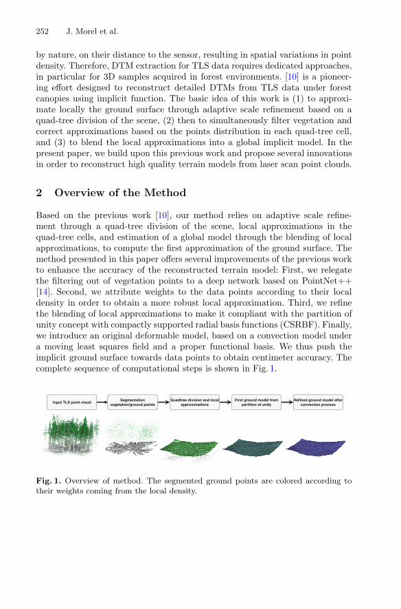
Based on the previous work [10], our method relies on adaptive scale refine-ment through a quad-tree division of the scene, local approximations in thequad-tree cells, and estimation of a global model through the blending of localapproximations, to compute the first approximation of the ground surface. Themethod presented in this paper offers several improvements of the previous workto enhance the accuracy of the reconstructed terrain model: First, we relegatethe filtering out of vegetation points to a deep network based on PointNet++[14]. Second, we attribute weights to the data points according to their localdensity in order to obtain a more robust local approximation. Third, we refinethe blending of local approximations to make it compliant with the partition ofunity concept with compactly supported radial basis functions (CSRBF). Finally,we introduce an original deformable model, based on a convection model undera moving least squares field and a proper functional basis. We thus push theimplicit ground surface towards data points to obtain centimeter accuracy. Thecomplete sequence of computational steps is shown in Fig. 1.

Input TLS point cloudSegmentation

vegetation/ground pointsQuadtree division and local

approximationsFirst ground model from

partition of unityRefined ground model after

convection process

Fig. 1. Overview of method. The segmented ground points are colored according totheir weights coming from the local density.

High Accuracy Terrain Reconstruction from Point Clouds 253

3 Filtering of Vegetation

3.1 Selection of Ground Points Using Deep Learning

In the estimation of ground surface from LiDAR point clouds, it is commonto first project the point cloud into a fine regular 2D (x,y) grid, of resolutionresMIN , and further select the points of minimum elevation in each cell. Theresulting point cloud is denoted Pmin. In order to ease the segmentation, weenriched each point of Pmin by geometric descriptors encoding the local linearityand planarity. In practice, we consider for each points its Cartesian coordinatesplus the averaged eigenvalues of the local covariance matrix of the 3D distributionof the KPCA neighbors, KPCA being defined by the user. In order to feed theseenriched point clouds into a convolutional architecture, we define a partition ofspace allowing splitting of an unordered 3D point cloud into overlapping fixedsize regions, each of them encoding the 3D local points distribution. In practice,we divide the point cloud Pmin into a regular 2D (x,y) grid, then distributecollocation points to the centroid of every occupied voxel. Then, we form eachbatch Bi by considering the 1024 nearest neighbors of each collocation point inthe (x,y) plane. These batches are designed to feed and train a deep learningmodel; this model eventually predicts a label for each point of each batch. Asbatches largely overlap, each input point belongs to several batches and thusreceive multiple predictions, one for every batch it belongs to. In the last step,we define a voting process to extract a final segmentation from the multiple votesper point. The resulting set of points denoted by P = {pi}i=1...N ⊂ R

3 servesas raw data for the proposed algorithm.

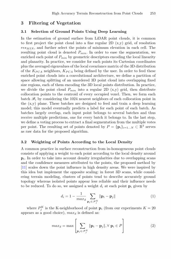
3.2 Weighting of Points According to the Local Density

A common practice in surface reconstruction from in-homogeneous point cloudsconsists of applying a weight to each point according to the local density aroundpi. In order to take into account density irregularities due to overlapping scansand the confidence measures attributed to the points, the proposed method by[11] scales down the point influence in high density areas. We were inspired bythis idea but implement the opposite scaling: in forest 3D scans, while consid-ering terrain modeling, clusters of points tend to describe accurately groundtopology whereas isolated points appear less reliable and their influence needsto be reduced. To do so, we assigned a weight di at each point pi given by

di = 1 − 1maxd

∑

pj∈PKj

‖pi − pj‖ (1)

where PKj is the K-neighborhood of point pi (from our experiments K = 20

appears as a good choice), maxd is defined as:

maxd = max

⎡

⎣∑

pj∈PKj

‖pi − pj‖,∀ pi ∈ P

⎤

⎦ (2)

254 J. Morel et al.

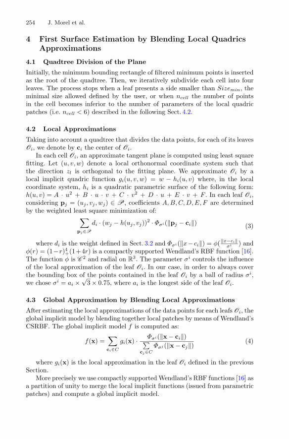
4 First Surface Estimation by Blending Local QuadricsApproximations

4.1 Quadtree Division of the Plane

Initially, the minimum bounding rectangle of filtered minimum points is insertedas the root of the quadtree. Then, we iteratively subdivide each cell into fourleaves. The process stops when a leaf presents a side smaller than Sizemin, theminimal size allowed defined by the user, or when ncell the number of pointsin the cell becomes inferior to the number of parameters of the local quadricpatches (i.e. ncell < 6) described in the following Sect. 4.2.

4.2 Local Approximations

Taking into account a quadtree that divides the data points, for each of its leavesOi, we denote by ci the center of Oi.

In each cell Oi, an approximate tangent plane is computed using least squarefitting. Let (u, v, w) denote a local orthonormal coordinate system such thatthe direction zl is orthogonal to the fitting plane. We approximate Oi by alocal implicit quadric function gi(u, v, w) = w − hi(u, v) where, in the localcoordinate system, hi is a quadratic parametric surface of the following form:h(u, v) = A · u2 + B · u · v + C · v2 + D · u + E · v + F . In each leaf Oi,considering pj = (uj , vj , wj) ∈ P, coefficients A,B,C,D,E, F are determinedby the weighted least square minimization of:

∑

pj∈P

di · (wj − h(uj , vj))2 · Φσi(‖pj − ci‖) (3)

where di is the weight defined in Sect. 3.2 and Φσi(‖x− ci‖) = φ(‖x−ci‖σi ) and

φ(r) = (1−r)4+(1+4r) is a compactly supported Wendland’s RBF function [16].The function φ is C 2 and radial on R

3. The parameter σi controls the influenceof the local approximation of the leaf Oi. In our case, in order to always coverthe bounding box of the points contained in the leaf Oi by a ball of radius σi,we chose σi = ai × √

3 × 0.75, where ai is the longest side of the leaf Oi.

4.3 Global Approximation by Blending Local Approximations

After estimating the local approximations of the data points for each leafs Oi, theglobal implicit model by blending together local patches by means of Wendland’sCSRBF. The global implicit model f is computed as:

f(x) =∑

ci∈C

gi(x) · Φσi(‖x − ci‖)∑cj∈C

Φσj (‖x − cj‖)(4)

where gi(x) is the local approximation in the leaf Oi defined in the previousSection.

More precisely we use compactly supported Wendland’s RBF functions [16] asa partition of unity to merge the local implicit functions (issued from parametricpatches) and compute a global implicit model.

High Accuracy Terrain Reconstruction from Point Clouds 255

5 Improvement of Surface Model with a ConvectionModel

Because occlusion phenomenon forces large quadtree cells, and thus coarser localapproximations, the first surface estimation described in Sect. 4 can be furtherimproved by being pushed closer to the data point. Inspired by the level-setsformulations [12,15] in the field of image processing, our method builds particu-larly on the work of Gelas [6] and describes the evolution of the surface driven bya time-dependent partial differential equation (PDE) where the so-called veloc-ity term reflects the 3D point cloud features. The level-set PDE is then solvedthrough a collocation method using CSRBF.

5.1 From Blended Quadrics Model to CSRBF Model

In order to both express the refined implicit surface and discretize the numericalproblem, we create a new base of functions. This basis is built according to thefollowing process: collocation centers are regularly distributed on a 3D grid, ofuser-defined resolution r, around the zero-levelset of the implicit function 4. Inorder to limit the number of collocations while allowing the surface to movein the vicinity of data points but, we decimate the clouds of collocation byremoving each center further than 2 × r from a data point or further than rfrom the zero-levelset. Considering Q the set of collocation, the basis of functionis then defined as the set of translates at each remaining collocation o ∈ Q ofWendland’s CSRBF Φro

(‖x − o‖) = φ(‖x−o‖ro

): where ro = r × √3 × 0.75.

First, we approximate the implicit function f defined in Eq. 4 in the newbasis Span{Φro

} as g(x) =∑

o∈Q

αo · Φro(‖x − o‖).

To retrieve {αo}o∈Q , we consider the system:∣∣∣∣∣∣∣∣

. . .Ao,o′

. . .

∣∣∣∣∣∣∣∣

∣∣∣∣∣∣∣∣

...αo

...

∣∣∣∣∣∣∣∣=

∣∣∣∣∣∣∣∣

...f(o′)

...

∣∣∣∣∣∣∣∣(5)

where o and o′ are two collocations, Ao,o′ = Φro(‖o′ − o‖) and the implicit

function f describing the blended quadrics model is expressed by Eq. 4. Thanksto the properties of Wendland’s CSRBF Φro

, the matrix of the Ao,o′ elements issparse, self-adjoint and positive definite. Thus, the system is inverted by usingthe LDLT Cholesky decomposition implemented by Eigen library.

5.2 Solving Convection Evolution Equation Using CSRBFCollocation

We define now the velocity vector V (p, t),p ∈ R3, t ∈ R, a function reflecting

the geometrical properties of the interface according to the data, and quantifyingthe local deformations over time. The velocity is actually computed at each

256 J. Morel et al.

collocation o ∈ O by minimization of an energy function inspired by the snakeapproaches introduced by Kass [8]. Indeed, we define the energy function ∀q ∈R

3, ξ(q) = γ · ξdata(q) + (1 − γ) · ξsurface(q), where ξdata(q) gives rise to samplepoints force and ξsurface(q) gives rise to external constraint forces. A weightingscalar parameter γ, defined by the user, adjusts the influence of both terms.

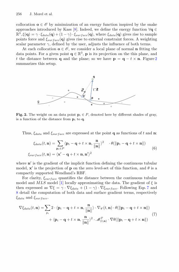
At each collocation o ∈ O, we consider a local plane of normal n fitting thedata points. For a given point q ∈ R

3, p is its projection on the this plane, andt the distance between q and the plane; so we have p = q − t × n. Figure 2summarizes this setup.

q

x'p

t . nn'

g

Fig. 2. The weight on an data point pi ∈ P , denoted here by different shades of gray,is a function of the distance from pi to q.

Thus, ξdata and ξsurface are expressed at the point q as functions of t and n:

ξdata(t,n) =∑

pi∈P

〈pi − q + t × n,n

‖n‖〉2 · θ(‖pi − q + t × n‖)

ξsurface(t,n) = 〈x′ − q + t × n,n′〉2(6)

where n′ is the gradient of the implicit function defining the continuous tubularmodel, x′ is the projection of p on the zero level-set of this function, and θ is acompactly supported Wendland’s RBF.

For clarity, ξsurface quantifies the distance between the continuous tubularmodel and MLS model [1] locally approximating the data. The gradient of ξ isthen expressed as ∇ξ = γ · ∇ξdata + (1 − γ) · ∇ξsurface. Following Eqs. 7 and8 detail the computation of both data and surface gradient terms, respectivelyξdata and ξsurface.

∇ξdata(t,n) =∑

pi

2 · 〈pi − q + t × n,n

‖n‖〉 · ∇G (t,n) · θ(‖pi − q + t × n‖)

+ 〈pi − q + t × n,n

‖n‖〉2 · M T(t,n) · ∇θ(‖pi − q + t × n‖)

(7)

High Accuracy Terrain Reconstruction from Point Clouds 257

where

⎧⎪⎪⎪⎪⎪⎪⎪⎪⎪⎪⎪⎨

⎪⎪⎪⎪⎪⎪⎪⎪⎪⎪⎪⎩

∇G (t,n) =

⎡

⎣1

‖n‖ · (I3 − n · nT

‖n‖2 ) · (pi − q) + t · n‖n‖

‖n‖

⎤

⎦

M(t,n) =

⎡

⎢⎣nx

I3 · t ny

nz

⎤

⎥⎦

∇θ(‖r‖) = (−20 · ‖r‖) · (1 − ‖r‖)3 · r‖r‖

The second gradient term is computed as:

∇ξsurface(t,n) = 2 · M T(t,n) · 〈x′ − q + t × n,n′〉 · n′ (8)

We retrieve (tmin,nmin), minimizing ξ(t,n) with the Fletcher-Reeves [5] con-jugate gradient algorithm available in the GSL library. The minimizer is initi-ated at the point q ∈ R

3 to (t0,n0) = (−−−−→q − x′ · n′,n′). From this minimization

process computed at each collocation o arises a deformation vector defined asvo = −tmin × nmin.

To push the surface to the data points according to the deformation vectorfield, we propose to follow a convection model as proposed by Osher [12]:

dg(p, t)dt

= vp ◦ ∇g(p, t) (9)

where vp is the deformation vector expressed at p, and ◦ is the element-wiseproduct. To solve Eq. 9, we assume that space and time are separable. We decom-pose g(p, t) = α(t) ·Φ(p) where Φ(p) is made of the basis functions values eval-uated at the point p and α(t) composed of the respective α values. Equation 9thus becomes the ordinary differential equation of evolution:

dα(t)dt

· Φ(p) = vp ◦ [α(t) · ∇Φ(p)] (10)

After the application of Euler’s method, Eq. 10 becomes:

α(t + τ) = α(t) − τ · Φ(p)−1 · H (t,p) (11)

where τ is the time step and H (t,p) = vp ◦ [α(t) · ∇Φ(p)]. The evolution ofthe CSRBF coefficients is finally given by Eq. 11. From this set of CSRBF, wecompute an implicit function and finally extract its zero level-set to produce theterrain surface model.

5.3 Re-normalization of Implicit Function

In order to prevent the apparition of new zero level components far away from theinitial surface, periodically reshaping the implicit function is a common strategy.In order to bound the function g defined in Sect. 5.1, hence its gradient ∇g, we

258 J. Morel et al.

bound the expansion of its coefficients αoc. In practice, inspired by [6], we bound

‖α(t)‖∞ if ‖α(t)‖∞ > β, where β is a positive constant. The evolution equationbecomes

⎧⎪⎨

⎪⎩

α(t + τ) = α(t) − τ · Φ(p)−1 · H (t,p)α(t + τ) = β

‖α(t+τ)‖∞· α(t + τ), if ‖α(t + τ)‖∞ > β

α(t + τ) = α(t + τ), otherwise(12)

5.4 Complexity

Using an octree data structure for the collocations layout, as advised by Wend-land [16], the matrix Φ(p) computation is O(NlogN) and the implicit functionevaluation g is O(logN). According to Botsch [2], the inversion of Φ(p) throughthe Cholesky factorization is O(nzf), where nzf is the number of nonzero fac-tors, which depends on the CSRBF center position and on the CSRBF supportsize. The cost of the re-normalization described in Sect. 5.3 is O(N).

6 Experiment and Validation

In order to train our deep learning model, labeled point clouds of forest plotmock-ups are required. To generate such data-sets, we simulate 3D point cloudsfrom artificial 3D terrains and trees models, as described in the followingSect. 6.1. As the accuracy of the terrain surface reconstructed by our methoddepends first on the efficiency of our deep network segmentation, we first mea-sured its ability to segment vegetation points from ground points on local minimaof simulated scenes. Section 6.3 describes the quantitative and qualitative resultsof terrain reconstruction on simulated and real TLS scans. Moreover, we evaluatethe improvement brought by the deformable model.

6.1 Training Data Generation

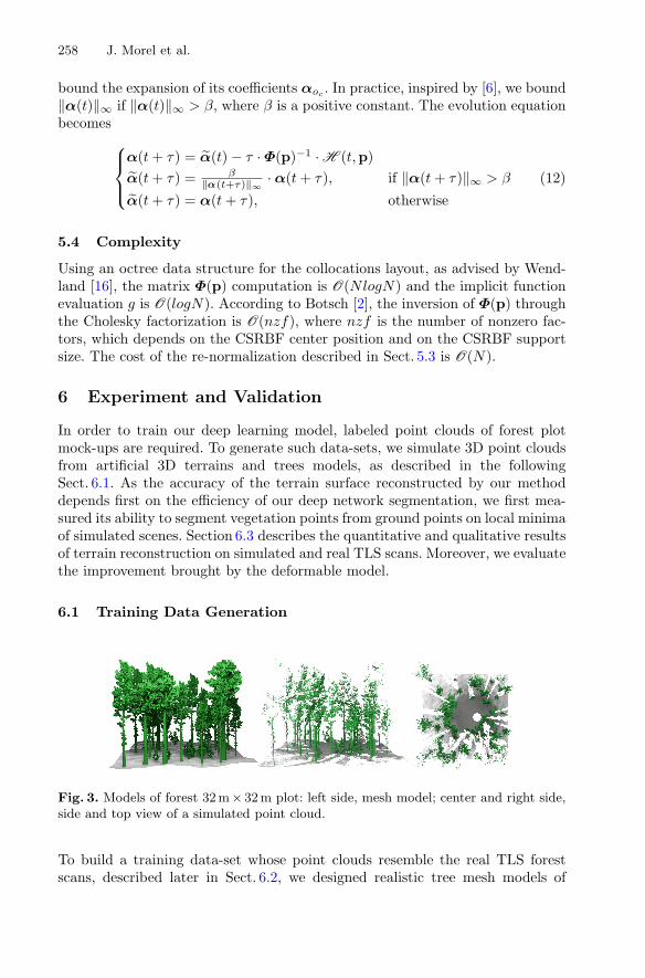
Fig. 3. Models of forest 32 m × 32m plot: left side, mesh model; center and right side,side and top view of a simulated point cloud.

To build a training data-set whose point clouds resemble the real TLS forestscans, described later in Sect. 6.2, we designed realistic tree mesh models of

High Accuracy Terrain Reconstruction from Point Clouds 259

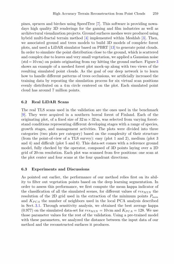
pines, spruces and birches using SpeedTree [7]. This software is providing nowa-days high quality 3D renderings for the gaming and film industries as well asarchitectural visualization projects. Ground surfaces meshes were produced usinghybrid multi-fractal terrain method [4] implemented within Meshlab [3]. Then,we associated ground and trees models to build 3D models of complete forestplots, and used a LiDAR simulator based on PBRT [13] to generate point clouds.In order to simulate the point distribution close to the ground, which is scatteredand complex due to leaves and very small vegetation, we applied a Gaussian noise(std = 10 cm) on points originating from ray hitting the ground surface. Figure 3shows an example of a meshed forest plot mock-up along with two views of theresulting simulated point clouds. As the goal of our deep network is to learnhow to handle different patterns of trees occlusions, we artificially increased thetraining data by repeating the simulation process for six virtual scan positionsevenly distributed on a 4 m circle centered on the plot. Each simulated pointcloud has around 7 million points.

6.2 Real LiDAR Scans

The real TLS scans used in the validation are the ones used in the benchmark[9]. They were acquired in a southern boreal forest of Finland. Each of theoriginating plot, of a fixed size of 32 m× 32 m, was selected from varying forest-stand conditions representing different developing stages with a range of species,growth stages, and management activities. The plots were divided into threecategories (two plots per category) based on the complexity of their structure(from the point-of-view of a TLS survey): easy (plot 1 and 2), medium (plot 3and 4) and difficult (plot 5 and 6). This data-set comes with a reference groundmodel, fully checked by the operator, composed of 3D points laying over a 2Dgrid of 20 cm resolution. Each plot was scanned from five positions: one scan atthe plot center and four scans at the four quadrant directions.

6.3 Experiments and Discussions

As pointed out earlier, the performance of our method relies first on its abil-ity to filter out vegetation points based on the deep learning segmentation. Inorder to assess this performance, we first compute the mean kappa indicator ofthe classification of all the simulated scenes, for different values of resMIN theresolution of the 2D grid used in the extraction of the minimum points Pmin

and KPCA the number of neighbors used in the local PCA analysis describedin Sect. 3.1. Through sensitivity analysis, we obtained the best average kappa(0.977) on the simulated data-set for resMIN = 10 cm and KPCA = 128. We usethose parameter values for the rest of the validation. Using a pre-trained modelwith these parameters, we analyzed the distance between the input data of ourmethod and the reconstructed surfaces it produces.

260 J. Morel et al.

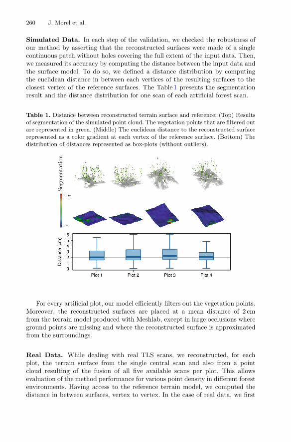
Simulated Data. In each step of the validation, we checked the robustness ofour method by asserting that the reconstructed surfaces were made of a singlecontinuous patch without holes covering the full extent of the input data. Then,we measured its accuracy by computing the distance between the input data andthe surface model. To do so, we defined a distance distribution by computingthe euclidean distance in between each vertices of the resulting surfaces to theclosest vertex of the reference surfaces. The Table 1 presents the segmentationresult and the distance distribution for one scan of each artificial forest scan.

Table 1. Distance between reconstructed terrain surface and reference: (Top) Resultsof segmentation of the simulated point cloud. The vegetation points that are filtered outare represented in green. (Middle) The euclidean distance to the reconstructed surfacerepresented as a color gradient at each vertex of the reference surface. (Bottom) Thedistribution of distances represented as box-plots (without outliers).

For every artificial plot, our model efficiently filters out the vegetation points.Moreover, the reconstructed surfaces are placed at a mean distance of 2 cmfrom the terrain model produced with Meshlab, except in large occlusions whereground points are missing and where the reconstructed surface is approximatedfrom the surroundings.

Real Data. While dealing with real TLS scans, we reconstructed, for eachplot, the terrain surface from the single central scan and also from a pointcloud resulting of the fusion of all five available scans per plot. This allowsevaluation of the method performance for various point density in different forestenvironments. Having access to the reference terrain model, we computed thedistance in between surfaces, vertex to vertex. In the case of real data, we first

High Accuracy Terrain Reconstruction from Point Clouds 261

extract the ground points using our deep learning network, then compute thedistance between the vertices of the reconstructed surface and the ground pointspackaged with the LiDAR scans. The results are shown in Table 2.

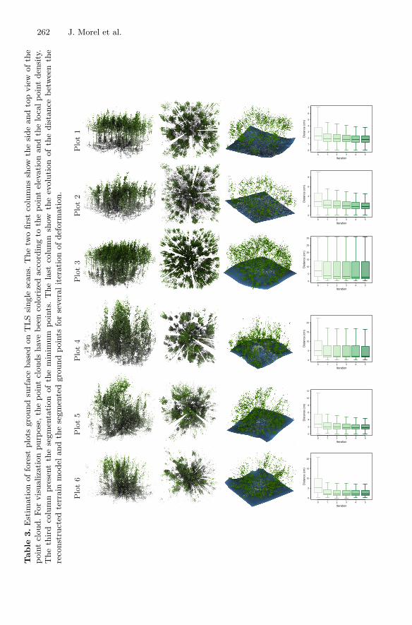
Finally, we analyzed the evolution of terrain model the iteration of deforma-tion, by measuring its distance distribution to the segmented ground points. Theresults are presented in Tables 3 and 4, for single and multiple scans respectively.

Table 2. Mean Hausdorff distance (cm) between reconstructed surface from sin-gle/multiple scan(s) and reference ground model.

Plot 1 2 3 4 5 6

Single - Mean Distance (cm) 6.04 5.82 22.23 26.89 12.85 21.76

Multiple - Mean Distance (cm) 2.58 3.14 5.93 8.27 2.88 7.17

As pointed out in the Table 2, the efficiency of our method to reconstruct aterrain model close to the reference depends on the terrain complexity and on thenature of the scans: for the simpler forest plots (1 and 2) single scans, our methodproduces accurate terrain models that are positioned 6 cm from the reference.Due to the missing points in the occlusion that expands with complexity, thisdistance increases for plots 3, 4, 5, and 6. However, in the case of multiple scans,the occlusion phenomenon lessens, which makes available anchor points allowingsharper terrain surfaces to be produced. In such cases, with our method, themean distances are around 3 cm on the simpler plot, and from 3 to 8 cm on amore complex topology.

In Tables 3 and 4, we analyzed the contribution of the deformation producedby the convection in the final accuracy of our terrain surfaces. For every plot,the mean of the distance distribution and its standard deviation decreases forboth single and multiple scans. The stronger drops occurs at the first iteration,the following ones remaining light in comparison. Except for plot 3 and 4 singlescans, the reconstructed surface sets at 2 cm on average from the segmentedground points after five iterations of convection.

The single scans of plots 3 and 4 highlight the limitation of our method:while the mean distance from the segmented ground points remained at 2 to3 cm, the distance distribution presents extreme values above 20 cm. This isdue to the failure of our deep learning model to correctly filter out vegetationpoints. Those two particular plots, while being scans from a single point presentsproblematic 3D points patterns, which vanish if scanned from multiple pointsof view. The forest mock-ups are crucial; they need to take proper account ofthe actual reality. Indeed, they are used to produce simulated data training anddetermine the quality of the segmentation, which is the first step of our methodand condition the reconstruction of the overall scene.

262 J. Morel et al.Table

3.E

stim

ati

on

offo

rest

plo

tsgro

und

surf

ace

base

don

TLS

single

scans.

The

two

firs

tco

lum

ns

show

the

side

and

top

vie

wofth

epoin

tcl

oud.For

vis

ualiza

tion

purp

ose

,th

epoin

tcl

ouds

hav

ebee

nco

lori

zed

acc

ord

ing

toth

epoin

tel

evati

on

and

the

loca

lpoin

tden

sity

.T

he

thir

dco

lum

npre

sent

the

segm

enta

tion

of

the

min

imum

poin

ts.

The

last

colu

mn

show

the

evolu

tion

of

the

dis

tance

bet

wee

nth

ere

const

ruct

edte

rrain

model

and

the

segm

ente

dgro

und

poin

tsfo

rse

ver

alit

erati

on

ofdef

orm

ati

on.

Plot1

Iteration

Dis

tanc

e (c

m)

0

1

2

3

4

5

6

7

0 1 2 3 4 5

Plot2

Iteration

Dis

tanc

e (c

m)

0

2

4

6

8

0 1 2 3 4 5

Plot3

Iteration

Dis

tanc

e (c

m)

0

5

10

15

20

25

30

0 1 2 3 4 5

Plot4

Iteration

Dis

tanc

e (c

m)

0

5

10

15

20

0 1 2 3 4 5

Plot5

Iteration

Dis

tanc

e (c

m)

0

2

4

6

8

10

12

0 1 2 3 4 5

Plot6

Iteration

Dis

tanc

e (c

m)

0

5

10

15

20

0 1 2 3 4 5

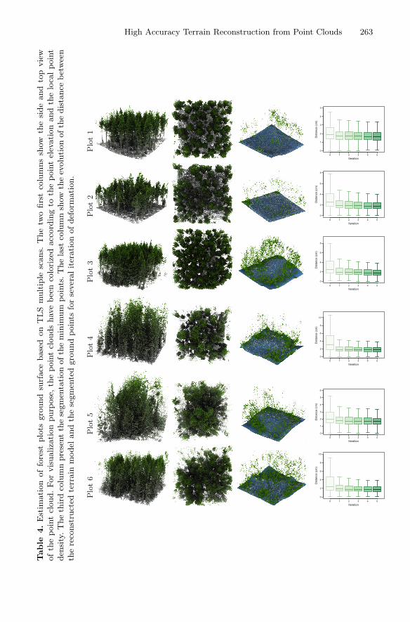
High Accuracy Terrain Reconstruction from Point Clouds 263Table

4.

Est

imati

on

of

fore

stplo

tsgro

und

surf

ace

base

don

TLS

mult

iple

scans.

The

two

firs

tco

lum

ns

show

the

side

and

top

vie

wofth

epoin

tcl

oud.For

vis

ualiza

tion

purp

ose

,th

epoin

tcl

ouds

hav

ebee

nco

lori

zed

acc

ord

ing

toth

epoin

tel

evati

on

and

the

loca

lpoin

tden

sity

.T

he

thir

dco

lum

npre

sent

the

segm

enta

tion

ofth

em

inim

um

poin

ts.T

he

last

colu

mn

show

the

evolu

tion

ofth

edis

tance

bet

wee

nth

ere

const

ruct

edte

rrain

model

and

the

segm

ente

dgro

und

poin

tsfo

rse

ver

alit

erati

on

ofdef

orm

ati

on.

Plot1

Iteration

Dis

tanc

e (c

m)

0

1

2

3

4

5

0 1 2 3 4 5

Plot2

Iteration

Dis

tanc

e (c

m)

0

2

4

6

8

0 1 2 3 4 5

Plot3

Iteration

Dis

tanc

e (c

m)

0

2

4

6

8

0 1 2 3 4 5

Plot4

Iteration

Dis

tanc

e (c

m)

0

2

4

6

8

10

0 1 2 3 4 5

Plot5

Iteration

Dis

tanc

e (c

m)

0

1

2

3

4

5

6

0 1 2 3 4 5

Plot6

Iteration

Dis

tanc

e (c

m)

0

2

4

6

8

10

0 1 2 3 4 5

264 J. Morel et al.

7 Conclusion

In this work, we propose an efficient method designed to recover terrain surfacemodel from 3D sample data acquired in forest environments. Our approach relieson deep learning to separate ground points from vegetation points. It handlesthe occlusion and builds a first approximation of the ground surface by blendingimplicit quadrics through the partition of unity principle. Then our method getsrid of the rigidity of the previous model by projecting it in a CSRBF basis beforedeforming it by convection. These contributions enable us to achieve state of theart performance in terrain reconstruction. In the future, it is worthwhile thinkingof how to design forest mock-ups adapted to train networks able to filter differentforest environments.

Acknowledgments. The authors would like to thank the reviewers for their thought-ful comments and efforts towards improving our manuscript and the Japan Society forthe Promotion of Science (JSPS) for providing Jules Morel fellowship.

References

1. Amenta, N., Kil, Y.J.: Defining point-set surfaces. In: ACM SIGGRAPH 2004Papers, pp. 264–270 (2004)

2. Botsch, M., Hornung, A., Zwicker, M., Kobbelt, L.: High-quality surface splattingon today’s GPUs. In: Proceedings Eurographics - IEEE VGTC Symposium Point-Based Graphics 2005, pp. 17–141. IEEE (2005)

3. Cignoni, P., Callieri, M., Corsini, M., Dellepiane, M., Ganovelli, F., Ranzuglia, G.:MeshLab: an open-source mesh processing tool. In: Eurographics Italian ChapterConference, vol. 2008, pp. 129–136 (2008)

4. Ebert, D.S., Musgrave, F.K.: Texturing & Modeling: A Procedural Approach. Mor-gan Kaufmann, Burlington (2003)

5. Fletcher, R., Reeves, C.M.: Function minimization by conjugate gradients. Com-put. J. 7(2), 149–154 (1964)

6. Gelas, A., Bernard, O., Friboulet, D., Prost, R.: Compactly supported radial basisfunctions based collocation method for level-set evolution in image segmentation.IEEE Trans. Image Process. 16(7), 1873–1887 (2007)

7. Interactive Data Visualization, Inc.: SpeedTree. IDV, 5446 Sunset Blvd. Suite 201Lexington, SC 29072 (2017). https://store.speedtree.com

8. Kass, M., Witkin, A., Terzopoulos, D.: Snakes: active contour models. Int. J. Com-put. Vis. 1(4), 321–331 (1988)

9. Liang, X., et al.: International benchmarking of terrestrial laser scanning approachesfor forest inventories. ISPRS J. Photogramm. Remote Sens. 144, 137–179 (2018)

10. Morel, J., Bac, A., Vega, C.: Terrain model reconstruction from terrestrial LiDARdata using radial basis functions. IEEE Comput. Graphics Appl. 37(5), 72–84(2017)

11. Ohtake, Y., Belyaev, A., Seidel, H.P.: 3D scattered data approximation with adap-tive compactly supported radial basis functions. In: Proceedings Shape ModelingApplications 2004, pp. 31–39. IEEE (2004)

12. Osher, S., Fedkiw, R.: Level Set Methods and Dynamic Implicit Surfaces, vol. 153.Springer, Heidelberg (2006)

High Accuracy Terrain Reconstruction from Point Clouds 265

13. Pharr, M., Jakob, W., Humphreys, G.: Physically Based Rendering: From Theoryto Implementation. Morgan Kaufmann, Burlington (2016)

14. Qi, C.R., Yi, L., Su, H., Guibas, L.J.: PointNet++: deep hierarchical feature learn-ing on point sets in a metric space. In: Advances in Neural Information ProcessingSystems, pp. 5099–5108 (2017)

15. Tsai, R., Osher, S., et al.: Review article: level set methods and their applicationsin image science. Commun. Math. Sci. 1(4), 1–20 (2003)

16. Wendland, H.: Scattered Data Approximation. Cambridge University Press, Cam-bridge (2005)