Scalable Surface Reconstruction

from Point Clouds with Extreme Scale and Density Diversity

Christian Mostegel Rudolf Prettenthaler Friedrich Fraundorfer Horst Bischof

Institute for Computer Graphics and Vision, Graz University of Technology ∗

{surname}@icg.tugraz.at

Abstract

In this paper we present a scalable approach for robustly

computing a 3D surface mesh from multi-scale multi-view

stereo point clouds that can handle extreme jumps of point

density (in our experiments three orders of magnitude). The

backbone of our approach is a combination of octree data

partitioning, local Delaunay tetrahedralization and graph

cut optimization. Graph cut optimization is used twice,

once to extract surface hypotheses from local Delaunay

tetrahedralizations and once to merge overlapping surface

hypotheses even when the local tetrahedralizations do not

share the same topology. This formulation allows us to ob-

tain a constant memory consumption per sub-problem while

at the same time retaining the density independent interpo-

lation properties of the Delaunay-based optimization. On

multiple public datasets, we demonstrate that our approach

is highly competitive with the state-of-the-art in terms of

accuracy, completeness and outlier resilience. Further, we

demonstrate the multi-scale potential of our approach by

processing a newly recorded dataset with 2 billion points

and a point density variation of more than four orders of

magnitude – requiring less than 9GB of RAM per process.

1. Introduction

In this work we focus on surface reconstruction from

multi-scale multi-view stereo (MVS) point clouds. These

point clouds receive increasing attention as their computa-

tion only requires simple 2D images as input. Thus the same

reconstruction techniques can be used for all kinds of 2D

images independent of the acquisition platform, including

satellites, airplanes, unmanned aerial vehicles (UAVs) and

terrestrial mounts. These platforms allow to capture a scene

in a large variety of resolutions (aka scale levels or levels of

details). A multicopter UAV alone can vary the level of de-

∗Results incorporated in this paper received funding from the European

Unions Horizon 2020 research and innovation programme under grant

agreement No 730294 and the EC FP7 project 3D-PITOTI (ICT-2011-

600545).

2.5 km 500 m

50 m 50 cm

5 cm

Figure 1. From kilometer to sub-millimeter. Our approach is capa-

ble to compute a consistently connected mesh even in the presence

of vast point density changes, while at the same time keeping a de-

finable constant peak memory usage.

tail by roughly two orders of magnitude. If the point clouds

from different acquisition platforms are combined, there is

no limit to the possible variety of point density and 3D un-

certainty. Further, the size of these point clouds can be im-

mense. State-of-the-art MVS approaches [10, 11, 12, 28]

compute 3D points in the order of the total number of ac-

quired pixels. This means that they generate 3D points in

the order of 107 per taken image with a modern camera. In

a few hours of time, it is thus possible to acquire images that

result in several billions of points.

Extracting a consistent surface mesh from this immense

amount of data is a non-trivial task, however, if such a mesh

could be extracted it would be a great benefit for virtual 3D

tourism. Instead of only being able to experience a city from

904

far away, it would then be possible to completely immerge

into the scene and experience cultural heritage in full detail.

However, current research in multi-scale surface recon-

struction focuses on one of two distinct goals (aside from

accuracy). One group (e.g. [8, 21]) focuses on scalabil-

ity through local formulations. The drawback of these ap-

proaches is that the completeness often suffers; i.e. many

holes can be seen in the reconstruction due to occlusions in

the scene, which reduces the usefulness for virtual reality.

The second group (e.g. [31, 33]) thus focuses on obtaining

a closed mesh through applying global methods. For ob-

taining the global solution, these methods require all data

at once, which sadly precludes them from being scalable.

Achieving both goals at once, scalability and a closed solu-

tion, might be impossible for arbitrary jumps in point den-

sity. The reason for this is that any symmetric neighborhood

on the density jump boundary can have more points in the

denser part than fit into memory, while having only a few

or even no points in the sparse part. However, scalability

requires independent sub-problems of limited size, while a

closed solution requires sufficient overlap for joining them

back together. To mitigate this problem, we formulate our

approach as a hybrid between global and local methods.

First, we separate the input data with a coarse octree,

where a leaf node typically contains thousands of points.

The exact amount of points is an adjustable parameter that

represents the trade-off between completeness and memory

usage. Within neighboring leaf nodes, we perform a lo-

cal Delaunay tetrahedralization and max-flow min-cut op-

timization to extract local surface hypotheses. This leads

to many surface hypotheses that partially share the same

base tetrahedralization, but also intersect each other in many

places. To resolve these conflicts between the hypotheses in

a non-volumetric manner, we propose a novel graph cut for-

mulation based on the individual surface hypotheses. This

formulation allows us to optimally fill holes which result

from local ambiguities and thus maximize the completeness

of the final surface. This allows us to handle point clouds

of any size with a constant memory footprint, where the ca-

pability to close holes can be traded off with the memory

usage. Thus we were able to generate a consistent mesh

from a point cloud with 2 billion points with a ground sam-

pling variation from 1m to 50µm using less than 9GB of

RAM per process (see Fig. 1 and video [24]).

2. Related Work

Surface reconstruction from point clouds is an exten-

sively studied topic and a general review can be found in [5].

In the following, we focus on the most relevant works with

respect to multi-scale point clouds and scalability.

Many surface reconstruction approaches rely on an

octree-structure for data handling. While it has been shown

by Kazhdan et al. [20] that consistent isosurfaces can be ex-

tracted from arbitrary octree structures, the vast scale differ-

ences imposed by multi-view stereo lead to new challenges

for octree-based approaches. Consequently, fixed depth ap-

proaches (e.g. [16, 19, 6]) are not well-suited for this kind

of input data. Thus, Muecke et al. [27] handle scale transi-

tions in computing meshes on multiple octree levels within

a crust of voxels around the data points and stitching the

partial solutions back together. However, this approach

is not scalable due to its global formulation. Fuhrmann

and Goesele [8] therefore propose a completely local sur-

face reconstruction approach, where they construct an im-

plicit function as the sum of basis functions. While this

approach is scalable from a theoretical stand point, the in-

terpolation capabilities are very limited due to a very small

support region. Furthermore, the pure local nature of the

approach is unable to cope with mutually supporting out-

liers (e.g. if one depthmap is misaligned with respect to

the other depthmaps), which occur quite often in practice

(see experiments). Kuhn et al. [21] reduce this problem by

checking for visibility conflicts in close proximity (10 vox-

els) of a measurement. Nevertheless, this approach still has

very limited interpolation capabilities compared to global

approaches. Recently, Ummenhofer and Brox [31] pro-

posed a global variational approach for surface reconstruc-

tion of large multi-scale point clouds. While they report that

they can process a billion points, the required memory foot

print for this problem size is already considerable (152 GB).

Aside from not being scalable due to the global formulation,

this approach also needs to balance the octree. As our ex-

periments demonstrate, this leads to severe problems if the

scale difference is too large.

Aside from octree-based approaches, there is also a con-

siderable amount of work that is based on the Delaunay

tetrahedralization of the 3D points [13, 15, 18, 22, 23, 33].

Opposed to octree-based approaches, the Delaunay tetra-

hedralization splits the space into uneven tetrahedra and

thus grants these approaches the unique capability to close

holes of arbitrary size for any point density. The key prop-

erty of these approaches is that they build a directed graph

based on the neighborhood of adjacent tetrahedra in the

Delaunay tetrahedralization. The energy terms within the

graph are then set according to rays between the cameras

and their corresponding 3D measurements. These visibility

terms make this type of approaches very accurate and robust

to outliers. The main differences between the approaches

mentioned above are how the smoothness terms are set and

what kind of post-processing is applied. One property that

all of these approaches share is that they are all based on

global graph cut optimization, which precludes them from

scalability. However, the complete resilience to changes in

point density makes these approaches ideal for multi-view

stereo surface reconstruction, which motivated us to scale

up this type of approaches.

905

c

p

(a) Delaunay Triangulation

αvis αvis αvis

αvis αvis

Sink/Inside

Source/Outside

(b) Dual Graph (c) Visibility Terms

Figure 2. Schematic of the base method [22] for graph cut optimization on the Delaunay tetrahedralization. In (a) we show a 2D cut

through the Delaunay tetrahedralization of a point cloud (small black dots). Additionally, we draw the ray going from camera c to a point

measurement p. In (b) we show the dual graph representation. The large black dots represent vertices in the dual graph and tetrahedra in

the primal tetrahedralization. The green dots represent imaginary tetrahedra which are connected to an infinity vertex. The small black

arrows are the directed edges of the dual graph (i.e. two edges for each facet in the Delaunay tetrahedralization). Additionally, each vertex

in the dual graph has one edge from the source and one edge to the sink (which are not plotted for better visibility). Each of the edges in

the graph has a capacity associated with it. This capacity is a combination of smoothness terms and visibility terms. In (c) we show how

the visibility terms are set for the ray drawn in (a), while the regularization terms are typically set on all edges (b).

3. Global Meshing by Labatut et al.

Our base method is a global meshing approach by La-

batut et al. [22], which requires a point cloud with vis-

ibility information as input (i.e. which point was recon-

structed using which cameras/images). With this data, they

first compute the Delaunay tetrahedralization of the point

cloud. This leads to a set of tetrahedra which are connected

to their neighbors through their facets. If the sampling is

dense enough, it has been shown that this tetrahedralization

contains a good approximation of the real surface [3]. Now

the main idea of [22] was to construct a dual graph represen-

tation of the Delaunay tetrahedralization and perform graph

cut optimization on this dual graph to extract a surface (a

visual representation of the dual graph is plotted in Fig. 2).

They formulated the problem such that after the optimiza-

tion each tetrahedron is either labeled as inside or outside.

This results in a watertight surface, which is the minimum

cut of the graph cut optimization and represents the transi-

tion between tetrahedra labeled as inside and outside.

The following optimization problem is solved by the

graph cut optimization to find the surface S:

argminS

Evis(S) + α · Esmooth(S) (1)

where Evis(S) is the data term and represents the penal-

ties for the visibility constraint violations (i.e. ray conflicts,

see Fig. 2.c). Esmooth(S) is the regularization term and is

the sum of all smoothness penalties across the surface. α

is a factor that balances the data and the regularization term

and thus it controls the degree of smoothness.

Many ways have been proposed to set these energy

terms [13, 15, 18, 22, 23, 33]. In an evaluation [25] on

the Strecha dataset [30], we found that a constant visibility

cost (Fig. 2.c) and a small constant regularization cost (per

edge/facets) lead to very accurate results. Thus we used this

energy formulation with α = 10−4 in all our experiments.

Note that this base energy formulation is not crucial for our

approach and can be replaced by other methods.

4. Making It Scale

To scale up the base method, it is necessary to first divide

the data into manageable pieces, which we achieve with an

unrestricted octree. On overlapping data subsets, we then

solve the surface extraction problem optimally and obtain

overlapping hypotheses. This brings us to the main con-

tribution of our work, the fusion of these hypotheses. The

main problem is that the property which gives the base ap-

proach its unique interpolation properties (i.e. the irregular

space division via Delaunay tetrahedralization) also makes

the fusion of the surface hypotheses a non-trivial problem.

We solve this problem by first collecting consistencies be-

tween the mesh hypotheses and then filling the remaining

holes via a second graph cut optimization on surface candi-

dates. In the following we explain all important steps.

Dividing and conquering the data. For dividing the

data, we use an octree, similar to other works in this

field [8, 20, 21, 27]. In contrast to these works, we treat

leaf nodes (aka voxels) of the tree differently. Instead of

treating a voxel as smallest unit, we only use it to reduce

the number points to a manageable size. We achieve this

by subdividing the octree nodes until the number of points

within each node is below a fixed threshold. As we want to

handle density jumps of arbitrary size, we do not restrict the

transition between neighboring voxels. This means that the

traditional local neighborhood is not well suited for com-

bining the local solutions, as this neighborhood can be very

large at the transition between scale levels. Instead, we

collect all unique voxel subsets, where each voxel in the

set touches the same voxel corner point (corner point, edge

and plane connections are respected). This limits the max-

imum subset size to 8 voxels. For each voxel subset, we

then compute a local Delaunay tetrahedralization and exe-

cute the base method (Sec. 3) to extract a surface hypothe-

sis. The resulting hypotheses strongly overlap each other in

most parts, but inconsistencies arise at the voxel boundaries.

In these regions, the tetrahedra topology strongly differs,

906

which results in a significant amount of artifacts and am-

biguity. For this reason, standard mesh repair approaches

such as [17, 4] are not applicable.

Building up a consistent mesh. In a first step, we collect

all triangles (within each voxel) which are shared among all

local solutions and add them to the combined solution. In

the following ”combined solution” will always refer to the

current state of the combined surface hypothesis. Note that

the initial combined solution is already a valid surface hy-

pothesis with many holes. Triangles which are part of the

combined solution are not revised by any subsequent steps.

Then we look for all triangles that span between two voxels

and are in the local solution of all voxel subsets that contain

these two voxels. If these triangles separate two final tetra-

hedra, we add them to the combined solution. In our case,

a final tetrahedron is a tetrahedron where the circumscrib-

ing sphere does not reach outside the voxel subset. After

this step, the combined solution typically contains a large

amount of holes at the voxel borders.

In the next step, we want to find edge-connected sets of

triangles (we will further refer to these sets as ”patches”)

with which we can close the holes in the combined solu-

tion. To create patch candidates, we search through the lo-

cal solutions. First, we remove triangles that would violate

the two-manifoldness of the combined solution (i.e. con-

necting a facet to an edge that already has two facets) or

would intersect the combined solution. Then we cluster all

remaining triangles in linear time to patches via their edge

connections. On a voxel basis, we now end up with many

patch candidates. While many candidates might be used to

close a hole, it happens that some of them are more suitable

than others. As the base approach produces a closed sur-

face for each voxel subset, this also means that it closes the

surface behind the scene. To avoid that such a patch is used

rather than one in the foreground, we rank the quality of a

patch by its centricity in the voxel subset. In other words,

we prefer patches which are far away from the outer bor-

der of the voxel subset, as the Delaunay tetrahedralization

is more stable in these regions. We compute the centricity

of a patch p as:

centricity(p) = 1−mini∈Ip

‖cp − i‖

rp, (2)

where cp is the centroid of the patch p, Ip is the set of inner

points (Fig. 3) of the voxel subset of p. rp is the distance

from the inner point to the farthest corner of the voxel in

which cp lies, which normalizes the centricity to [0,1].

For each voxel, we now try to fit the candidate patches

in descending order, while ensuring that the outer boundary

completely connects to the combined solution without vi-

olating the two-manifoldness or intersecting the combined

solution. If such a patch is found it is added to the com-

(a) (b) (c) (d)

Figure 3. For computing the centricity, we consider 4 types of in-

ner points: (a) Within a voxel, (b) on the plane between 2 voxels,

(c) on the edge between 4 voxels (d) on the point between 8 voxels.

Patch Candidate

Partially Closed Surface

Minimum Cut

Source

Sink

Figure 4. Hole filling via graph cut. We transform the mesh into

nodes (from 3D triangles) and weighted directed edges (from 3D

edges). In yellow we show triangles of the combined solution

which are relevant for our optimization, whereas the blue triangles

are not relevant. The orange triangles represent the patch candidate

for hole filling (Tp). The capacity of the graph edges corresponds

to the 3D edge length (colors show the capacity). Only the edges

from the source (black edges) have infinite capacity. The dashed

red line shows the minimum cut of this example.

bined solution. Thus this step closes holes which can be

completely patched with a single local solution.

Hole filling via graph cut To deal with parts of the scene

where the local Delaunay tetrahedralizations are very incon-

sistent, we propose a graph cut formulation on the triangles

of a patch candidate. For efficiency, this graph cut operates

only on surface patches for which the visibility terms have

already been evaluated by the first graph cut. The idea be-

hind the formulation is to minimize the total length of the

outer mesh boundary.

First, we rank all candidate patches by centricity. For

the best patch candidate, we extract all triangles in the com-

bined solution which share an edge connection with the

patch. The edges connecting the combined solution with the

patch define the ”hole” which we aim to close or minimize

(we refer to this set of edges as Eh and the corresponding

set of triangles as Th). Within the set of patch triangles (Tp),

we now want to extract the optimal subset of triangles (T∗)

such that the overall outer edge length is minimized:

T∗ = argminTi⊆Tp

∑

e∈Ei

‖e‖, (3)

where Ei is the set of outer edges (i.e. edges only shared by

one triangle) defined through the triangle subset Ti and Eh.

We achieve this minimization with the following graph

formulation (see also Fig. 4). For each triangle in the hole

907

set Th and the patch Tp we insert a node in the graph. Then

we insert edges with infinite capacity from the source to all

triangles/nodes in Th (to force this set of triangles to be part

of the solution). All triangles in Th are then connected to

their neighbors in Tp with directed edges, where the capac-

ity of the edge in the graph corresponds to the edge length

in 3D. Similarly, we insert two graph edges for each pair of

neighboring triangles in Tp, where the capacity is also equal

to the edge length. Finally, we insert a graph edge for each

outer triangle (i.e. all triangles with less than three neigh-

bors). These edges are connected to the sink and their ca-

pacity is the sum of all outer edges of the triangle. Through

this formulation, the graph cut optimization minimizes the

total length of the remaining boundary. After the optimiza-

tion, all triangles which are needed for the optimal bound-

ary reduction are contained in the source set of the graph.

These triangles are added to the combined solution and the

process is repeated with the next patch candidate.

5. Experiments

We split our experiments into three parts. First, we

present qualitative results on a publicly available multi-

scale dataset [9] and a new cultural heritage dataset with

an extreme density diversity (from 1m to 50µm). Second,

we evaluate our approach quantitatively on the Middlebury

dataset [29] and the DTU dataset [1]. Third, we assess the

breakdown behavior of our approach in a synthetic experi-

ment, where we iteratively increase the point density ratio

between neighboring voxels up to a factor of 4096.

For all our experiments, we use the same set of parame-

ters. The most interesting parameter is the maximum num-

ber of points per voxel (further referred to as ”leaf size”),

which represents the trade-off between completeness and

memory usage. We set this parameter to 128k points, which

keeps the memory consumption per process below 9GB.

Only in our first experiment (Citywall), we vary this param-

eter to assess its sensitivity (which turns out to be very low).

As detailed in our technical report [25], the base method

per se is not able to handle Gaussian noise without a loss of

accuracy. Thus, we apply simple pre- and post-processing

steps for the reduction of Gaussian noise. As pre-processing

step, we apply scale sensitive point fusion. Points are itera-

tively and randomly drawn from the set of all points within

a voxel. For each drawn point, we fuse the k-nearest neigh-

bors within a radius of 3 times the point scale (points cannot

be fused twice). This step can be seen as the non-volumetric

equivalent to the fusion of points on a fixed voxel grid. The

k-nn criterion only prohibits that uncertain points delete

too many more accurate points. We select k such that all

points of similar scale within the radius are fused if no sig-

nificantly finer scale is present (leading to k = 20). As

post-processing, we apply two iterations of HC-Laplacian

smoothing [32]. Both, post- and pre-processing, are com-

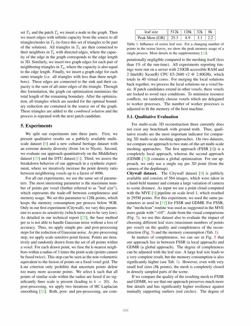
leaf size 512k 128k 32k 8k

Peak Mem [GB] 25.3 8.9 3.1 2.2

Table 1. Influence of octree leaf size. For a changing number of

points in the octree leaves, we show the peak memory usage of a

single process. More details in the supplementary [24].

putationally negligible compared to the meshing itself (less

than 1% of the run-time). All experiments reporting tim-

ings were run on a server with 210GB accessible RAM and

2 Intel(R) Xeon(R) CPU E5-2680 v2 @ 2.80GHz, which

totals in 40 virtual cores. For merging the local solutions

back together, we process the local solutions on a voxel ba-

sis. If patch candidates extend in other voxels, these voxels

are locked to avoid race conditions. To minimize resource

conflicts, we randomly choose voxels which are delegated

to worker processes. The number of worker processes is

adjusted to fit the memory of the host machine.

5.1. Qualitative Evaluation

For multi-scale 3D reconstruction there currently does

not exist any benchmark with ground truth. Thus, quali-

tative results are the most important indicator for compar-

ing 3D multi-scale meshing approaches. On two datasets,

we compare our approach to two state-of-the-art multi-scale

meshing approaches. The first approach (FSSR [8]) is a

completely local approach, whereas the second approach

(GDMR [31]) contains a global optimization. For our ap-

proach, we only use a single ray per 3D point (from the

camera of the depthmap).

Citywall dataset. The Citywall dataset [9] is publicly

available and consists of 564 images, which were taken in

a hand-held manner and contain a large variation of camera

to scene distance. As input we use a point cloud computed

with the MVE [9] pipeline on scale level 1, which resulted

in 295M points. For this experiment, we used the same pa-

rameters as used in [31] for FSSR and GDMR. For FSSR,

the ”meshclean” routine was used as suggested in the MVE

users guide with ”-t10”. Aside from the visual comparisons

(Fig. 5), we use this dataset also to evaluate the impact of

choosing different leaf sizes (maximum numbers of points

per voxel) on the quality and completeness of the recon-

struction (Fig. 5) and the memory consumption (Tab. 1).

In matters of completeness, we can see in Fig. 5 that

our approach lies in between FSSR (a local approach) and

GDMR (a global approach). The degree of completeness

can be adjusted with the leaf size. A large leaf size leads to

a very complete result, but the memory consumption is also

significantly higher (see Tab. 1). However, even with very

small leaf sizes (8k points), the mesh is completely closed

in densely sampled parts of the scene.

If we compare the quality of the resulting mesh to FSSR

and GDMR, we see that our approach preserves much more

fine details and has significantly higher resilience against

mutually supporting outliers (red circles). The degree of

908

resilience declines gracefully when the leaf size becomes

lower, and even for 8k points the output is, in this respect,

at least as good as FSSR and GDMR. The drawback of our

method is that the Gaussian noise level is somewhat higher

compared to the other approaches, which could be reduced

with more smoothing iterations.

Valley dataset. The Valley dataset is a cultural heritage

dataset, where the images were taken on significantly dif-

ferent scale levels. The most coarse scale was recorded

with a manned and motorized hang glider, the second scale

level with a fixed wing UAV (unmanned aerial vehicle),

the third with an autonomous octocopter UAV [26] and the

finest scale with a terrestrial stereo setup [14]. Each scale

was reconstructed individually and then geo-referenced us-

ing offline differential GPS measurements of ground con-

trol points (GCPs), total station measurements of further

GCPs and a prism on the stereo setup [2]. The relative

alignment was then fine-tuned with ICP (iterative closest

point). On each scale level we densified the point cloud

using SURE [28], which was mainly developed for aerial

reconstruction and is therefore ideally suited for this data.

We compute the point scale for SURE analog to MVE as

the average 3D distance from a depthmap value to its neigh-

bors (4-neighborhood). The resulting point clouds have the

following size and ground sampling distance: Stereo setup

(1127M points @ 43-47µm), octocopter UAV (46M points

@ 3.5-15mm), fixed wing UAV (162M points @ 3-5cm)

and hang glider (572M points @ 10-100cm), which sums up

to 1.9 billion points in total. This dataset is available [24].

On this dataset, FSSR and GDMR were executed with

the standard parameters, which also obtained the ”best” re-

sults for SURE input on the DTU dataset (see Sec. 5.2).

However, both approaches ran out of memory with these

parameters on the evaluation machine with 210 GB RAM.

To obtain any results for comparison we increased the scale

parameter (in multiples of two) until the approaches could

be successfully executed, which resulted in a scaling fac-

tor of 4 for FSSR and GDMR. The second problem of the

reference implementations is that they use a maximum oc-

tree depth of 21 levels for efficient voxel indexing, but this

dataset requires a greater depth. Thus both implementations

ignore the finest scale level. To still evaluate the transition

capabilities between octocopter and stereo scale, we also

executed both approaches on only these two scale levels

(marked as ”only subset”). The overall runtimes were 1.5

days for GDMR, 0.5 days for FSSR and 9 days for our ap-

proach. One has to be keep in mind that FSSR and GDMR

had two octree levels less (data reduction between 16 and

64), additionally to throwing away the lowest scale (half

of the points). Furthermore, our approach only required

119GB of memory with 16 processes, whereas GDMR re-

quired 150GB and FSSR 170GB, despite the large data re-

duction. Per process our approach once again required less

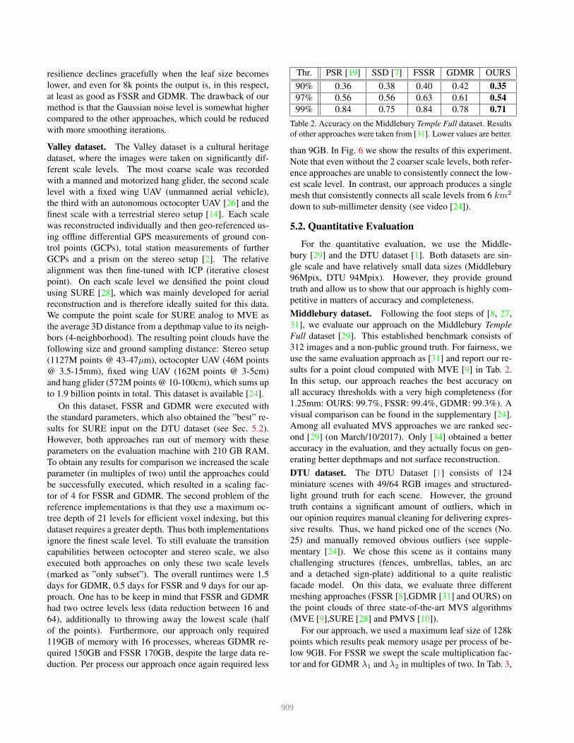
Thr. PSR [19] SSD [7] FSSR GDMR OURS

90% 0.36 0.38 0.40 0.42 0.35

97% 0.56 0.56 0.63 0.61 0.54

99% 0.84 0.75 0.84 0.78 0.71

Table 2. Accuracy on the Middlebury Temple Full dataset. Results

of other approaches were taken from [31]. Lower values are better.

than 9GB. In Fig. 6 we show the results of this experiment.

Note that even without the 2 coarser scale levels, both refer-

ence approaches are unable to consistently connect the low-

est scale level. In contrast, our approach produces a single

mesh that consistently connects all scale levels from 6 km2

down to sub-millimeter density (see video [24]).

5.2. Quantitative Evaluation

For the quantitative evaluation, we use the Middle-

bury [29] and the DTU dataset [1]. Both datasets are sin-

gle scale and have relatively small data sizes (Middlebury

96Mpix, DTU 94Mpix). However, they provide ground

truth and allow us to show that our approach is highly com-

petitive in matters of accuracy and completeness.

Middlebury dataset. Following the foot steps of [8, 27,

31], we evaluate our approach on the Middlebury Temple

Full dataset [29]. This established benchmark consists of

312 images and a non-public ground truth. For fairness, we

use the same evaluation approach as [31] and report our re-

sults for a point cloud computed with MVE [9] in Tab. 2.

In this setup, our approach reaches the best accuracy on

all accuracy thresholds with a very high completeness (for

1.25mm: OURS: 99.7%, FSSR: 99.4%, GDMR: 99.3%). A

visual comparison can be found in the supplementary [24].

Among all evaluated MVS approaches we are ranked sec-

ond [29] (on March/10/2017). Only [34] obtained a better

accuracy in the evaluation, and they actually focus on gen-

erating better depthmaps and not surface reconstruction.

DTU dataset. The DTU Dataset [1] consists of 124

miniature scenes with 49/64 RGB images and structured-

light ground truth for each scene. However, the ground

truth contains a significant amount of outliers, which in

our opinion requires manual cleaning for delivering expres-

sive results. Thus, we hand picked one of the scenes (No.

25) and manually removed obvious outliers (see supple-

mentary [24]). We chose this scene as it contains many

challenging structures (fences, umbrellas, tables, an arc

and a detached sign-plate) additional to a quite realistic

facade model. On this data, we evaluate three different

meshing approaches (FSSR [8],GDMR [31] and OURS) on

the point clouds of three state-of-the-art MVS algorithms

(MVE [9],SURE [28] and PMVS [10]).

For our approach, we used a maximum leaf size of 128k

points which results peak memory usage per process of be-

low 9GB. For FSSR we swept the scale multiplication fac-

tor and for GDMR λ1 and λ2 in multiples of two. In Tab. 3,

909

Figure 5. Visual comparison of the citywall dataset [9]. From left to right, we first show the output of our approach with different values for

the maximum number of points per octree node (ranging from 512k to only 8k). Then we show the results of the state-of-the-art methods

GDMR [31] and FSSR [8]. The first four rows show similar view points as used in [31] for a fair comparison. The regions encircled in red

highlight one of the benefits of our method, i.e. preserving small details while being highly resilient against mutually supporting outliers.

Concerning the maximum leaf size, larger leaf sizes lead to more complete results with our approach (blue circles). However, our method

is able to handle even very small leaf sizes (8k points) gracefully, with only a slight increase of holes and outliers.

Figure 6. Valley dataset. From top to bottom, we traverse the vast scale changes of the reconstruction (from 6 km2 down to 50 µm

sampling distance). From left to right, we show our results, GDMR [31] and FSSR [8]; with and without color. As GDMR and FSSR are

both not able handle the vast scale difference, we also show the results computed only with the point clouds of the octocopter UAV and

the stereo setup as input (red boxes). In the last row, we show all meshes as wire frames to highlight the individual triangles (yellow boxes

show the visualized region). Note that our approach consistently connects all scales.

910

MVE MeanAcc MedAcc MeanCom MedCom

FSSR 0.673 (2) 0.396 (3) 0.430 (3) 0.239 (1)

GDMR 1.013 (3) 0.275 (2) 0.423 (2) 0.284 (3)

OURS 0.671 (1) 0.262 (1) 0.423 (1) 0.279 (2)

SURE MeanAcc MedAcc MeanCom MedCom

FSSR 1.044 (1) 0.490 (3) 0.431 (1) 0.257 (1)

GDMR 1.099 (2) 0.301 (1) 0.519 (3) 0.357 (2)

OURS 1.247 (3) 0.365 (2) 0.509 (2) 0.368 (3)

PMVS MeanAcc MedAcc MeanCom MedCom

FSSR 0.491 (1) 0.318 (1) 0.624 (3) 0.395 (3)

GDMR 0.996 (3) 0.355 (3) 0.537 (1) 0.389 (1)

OURS 0.626 (2) 0.341 (2) 0.567 (2) 0.390 (2)

Table 3. Accuracy and completeness on scene 25 of DTU

Dataset [1]. We evaluate three different meshing approaches

(FSSR [8],GDMR [31] and OURS) on the point clouds of three

different MVS approaches (MVE [9],SURE [28] and PMVS [10]).

For all evaluated factors (mean/median accuracy and mean/median

completeness) lower values are better. In brackets we show the rel-

ative rank.

we compare our approach to the ”best” values of FSSR and

GDMR. With ”best” we mean that the sum of the median

accuracy and completeness is minimal over all evaluated

parameters. A table with all evaluated parameters can be

found in the supplementary [24].

If we take a look at the results, we can see that the relative

performance of each approach is strongly influenced by the

input point cloud. For PMVS input, our approach is ranked

second in all factors, while FSSR obtains a higher accuracy

at the cost of lower completeness and GDMR higher com-

pleteness at the cost of lower accuracy. On SURE input, our

approach performs worse than the other two. Note that in

this scene, SURE produces a great amount of mutually con-

sistent outliers through extrapolation in texture-less regions.

These outliers cannot be resolved with the visibility term as

all cameras observe the scene from the same side. For MVE

input, our approach achieves the best rank in nearly all eval-

uated factors.

5.3. Breakdown Analysis

In this experiment, we evaluate the limits of our ap-

proach with respect to point density jumps. Thus we con-

struct an artificial worst case scenario, i.e. a scenario where

the density change happens exactly at the voxel border. Our

starting point is a square plane where we sample 2.4 mil-

lion points and to which we add some Gaussian noise in

the z-axis. The points are connected to 4 virtual cameras

(visibility links), which are positioned fronto parallel to the

plane. Then we subsequently reduce the number of points

in the center of the plane by a factor 2 until we detect the

first holes in the reconstruction (which happened at a reduc-

tion of 64). Then we reduce the point density by a factor 4

until a density ratio of 4096.

Figure 7. Synthetic breakdown experiment. From left to right, we

reduce the number of points in the center of the square. The num-

ber in the top row shows the density ratio between the outer parts

of the square and the inner part. From top to bottom, we show the

different steps of our approach ((1) collecting consistencies, (2)

closing holes with patches and (3) graph cut-based hole filling).

We colored the image background red to highlight the holes in the

reconstruction. Note that the after the first step, many holes exist

exactly on the border of the octree nodes, which our further steps

close or at least reduce.

In Fig. 7 we show the most relevant parts of the exper-

iment. Up to a density ratio of 32, our approach is able to

produce a hole-free mesh as output. If we compare this to

a balanced octree (where the relative size of adjacent vox-

els is limited to a factor two), we can perfectly cope with 8

times higher point densities. When the ratio becomes even

higher, the number of holes at the transition rises gradually.

In Fig. 7, we can see that graph cut optimization is able to

reduce the size of the remaining holes significantly, even

for a density ratio of 4k. This means that even for extreme

density ratios of over 3 orders we can still provide a result,

albeit one that contains a few holes at the transition.

6. Conclusion

In this paper we presented a hybrid approach between

volumetric and Delaunay-based surface reconstruction ap-

proaches. This formulation gives our approach the unique

ability to handle multi-scale point clouds of any size with a

constant memory usage. The number of points per voxel is

the only relevant parameter of our approach, which directly

represents the trade-off between completeness and memory

consumption. In our experiments, we were thus able to re-

construct a consistent surface mesh on a dataset with 2 bil-

lion points and a scale variation of more than 4 orders of

magnitude requiring less than 9GB of RAM per process.

Our other experiments demonstrated that, despite the low

memory usage, our approach is still extremely resilient to

outlier fragments, vast scale changes and highly competi-

tive in accuracy and completeness with the state-of-the-art

in multi-scale surface reconstruction.

911

References

[1] H. Aanæs, R. R. Jensen, G. Vogiatzis, E. Tola, and A. B.

Dahl. Large-scale data for multiple-view stereopsis. Inter-

national Journal of Computer Vision, pages 1–16, 2016. 5,

6, 8

[2] C. Alexander, A. Pinz, and C. Reinbacher. Multi-scale 3d

rock-art recording. Digital Applications in Archaeology and

Cultural Heritage, 2(23):181 – 195, 2015. Digital imaging

techniques for the study of prehistoric rock art. 6

[3] N. Amenta and M. Bern. Surface reconstruction by Voronoi

filtering. In Proceedings of the fourteenth annual symposium

on Computational geometry (SCG), 1998. 3

[4] M. Attene. Direct repair of self-intersecting meshes. Graph-

ical Models, 76(6):658 – 668, 2014. 4

[5] M. Berger, A. Tagliasacchi, L. M. Seversky, P. Alliez, J. A.

Levine, A. Sharf, and C. T. Silva. State of the Art in Sur-

face Reconstruction from Point Clouds. In S. Lefebvre and

M. Spagnuolo, editors, Eurographics 2014 - State of the Art

Reports. The Eurographics Association, 2014. 2

[6] M. Bolitho, M. Kazhdan, R. Burns, and H. Hoppe. Mul-

tilevel streaming for out-of-core surface reconstruction. In

Proceedings of the Fifth Eurographics Symposium on Ge-

ometry Processing, SGP ’07, pages 69–78, Aire-la-Ville,

Switzerland, Switzerland, 2007. Eurographics Association.

2

[7] F. Calakli and G. Taubin. Ssd: Smooth signed dis-

tance surface reconstruction. Computer Graphics Forum,

30(7):1993–2002, 2011. 6

[8] S. Fuhrmann and M. Goesele. Floating scale surface recon-

struction. ACM Trans. Graph., 33(4):46:1–46:11, July 2014.

2, 3, 5, 6, 7, 8

[9] S. Fuhrmann, F. Langguth, and M. Goesele. Mve-a mul-

tiview reconstruction environment. In Proceedings of the

Eurographics Workshop on Graphics and Cultural Heritage

(GCH), volume 6, page 8, 2014. 5, 6, 7, 8

[10] Y. Furukawa and J. Ponce. Accurate, dense, and robust multi-

view stereopsis. IEEE Transactions on Pattern Analysis and

Machine Intelligence, 32(8), 2010. 1, 6, 8

[11] S. Galliani, K. Lasinger, and K. Schindler. Massively par-

allel multiview stereopsis by surface normal diffusion. In

International Conference on Computer Vision (ICCV), pages

873–881, 2015. 1

[12] M. Goesele, N. Snavely, B. Curless, H. Hoppe, and S. M.

Seitz. Multi-view stereo for community photo collections. In

International Conference on Computer Vision (ICCV), pages

1–8, Oct 2007. 1

[13] V. Hiep, R. Keriven, P. Labatut, and J.-P. Pons. To-

wards high-resolution large-scale multi-view stereo. In IEEE

Conference on Computer Vision and Pattern Recognition

(CVPR), pages 1430–1437, June 2009. 2, 3

[14] T. Holl and A. Pinz. Cultural heritage acquisition:

Geometry-based radiometry in the wild. In 2015 Interna-

tional Conference on 3D Vision, pages 389–397, Oct 2015.

6

[15] C. Hoppe, M. Klopschitz, M. Donoser, and H. Bischof.

Incremental surface extraction from sparse structure-from-

motion point clouds. In British Machine Vision Conference

(BMVC), pages 94–1, 2013. 2, 3

[16] A. Hornung and L. Kobbelt. Robust reconstruction of wa-

tertight 3d models from non-uniformly sampled point clouds

without normal information. In Proceedings of the Fourth

Eurographics Symposium on Geometry Processing, SGP

’06, pages 41–50, Aire-la-Ville, Switzerland, Switzerland,

2006. Eurographics Association. 2

[17] A. Jacobson, L. Kavan, and O. Sorkine-Hornung. Robust

inside-outside segmentation using generalized winding num-

bers. ACM Trans. Graph., 32(4):33:1–33:12, July 2013. 4

[18] M. Jancosek and T. Pajdla. Multi-view reconstruction pre-

serving weakly-supported surfaces. In IEEE Conference on

Computer Vision and Pattern Recognition (CVPR), pages

3121–3128, June 2011. 2, 3

[19] M. Kazhdan, M. Bolitho, and H. Hoppe. Poisson surface

reconstruction. In Proceedings of the fourth Eurographics

symposium on Geometry processing, volume 7, 2006. 2, 6

[20] M. Kazhdan, A. Klein, K. Dalal, and H. Hoppe. Uncon-

strained isosurface extraction on arbitrary octrees. In Pro-

ceedings of the Fifth Eurographics Symposium on Geometry

Processing, SGP ’07, pages 125–133, Aire-la-Ville, Switzer-

land, Switzerland, 2007. Eurographics Association. 2, 3

[21] A. Kuhn, H. Hirschmuller, D. Scharstein, and H. Mayer. A tv

prior for high-quality scalable multi-view stereo reconstruc-

tion. International Journal of Computer Vision, pages 1–16,

2016. 2, 3

[22] P. Labatut, J.-P. Pons, and R. Keriven. Efficient multi-view

reconstruction of large-scale scenes using interest points, de-

launay triangulation and graph cuts. In International Con-

ference on Computer Vision (ICCV), pages 1–8, Oct 2007. 2,

3

[23] P. Labatut, J.-P. Pons, and R. Keriven. Robust and efficient

surface reconstruction from range data. Computer Graphics

Forum, 28(8):2275–2290, 2009. 2, 3

[24] C. Mostegel, R. Prettenthaler, F. Fraundorfer, and

H. Bischof. Scalable Surface Reconstruction from

Point Clouds with Extreme Scale and Density Diversity:

Supplementary material including dataset and video.

https://www.tugraz.at/institute/icg/

Media/mostegel_cvpr17, 2017. 2, 5, 6, 8

[25] C. Mostegel and M. Rumpler. Robust Surface Re-

construction from Noisy Point Clouds using Graph

Cuts. Technical report, Graz University of Technol-

ogy, Institute of Computer Graphics and Vision, June

2012. https://www.tugraz.at/institute/icg/

Media/mostegel_2012_techreport. 3, 5

[26] C. Mostegel, M. Rumpler, F. Fraundorfer, and H. Bischof.

Uav-based autonomous image acquisition with multi-view

stereo quality assurance by confidence prediction. In The

IEEE Conference on Computer Vision and Pattern Recogni-

tion (CVPR) Workshops, June 2016. 6

[27] P. Muecke, R. Klowsky, and M. Goesele. Surface reconstruc-

tion from multi-resolution sample points. In Proceedings of

Vision, Modeling, and Visualization (VMV), 2011. 2, 3, 6

[28] M. Rothermel, K. Wenzel, D. Fritsch, and N. Haala. SURE:

Photogrammetric Surface Reconstruction from Imagery. In

Proceedings LC3D Workshop, 2012. 1, 6, 8

912

[29] S. M. Seitz, B. Curless, J. Diebel, D. Scharstein, and

R. Szeliski. A comparison and evaluation of multi-view

stereo reconstruction algorithms. In IEEE Conference on

Computer Vision and Pattern Recognition (CVPR), vol-

ume 1, pages 519–528. IEEE, 2006. http://vision.

middlebury.edu/mview/eval/. 5, 6

[30] C. Strecha, W. von Hansen, L. Van Gool, P. Fua, and

U. Thoennessen. On benchmarking camera calibration and

multi-view stereo for high resolution imagery. In IEEE

Conference on Computer Vision and Pattern Recognition

(CVPR), pages 1–8, June 2008. 3

[31] B. Ummenhofer and T. Brox. Global, dense multiscale re-

construction for a billion points. In International Conference

on Computer Vision (ICCV), December 2015. 2, 5, 6, 7, 8

[32] J. Vollmer, R. Mencl, and H. Mueller. Improved laplacian

smoothing of noisy surface meshes. In Computer Graphics

Forum, volume 18, pages 131–138. Wiley Online Library,

1999. 5

[33] H.-H. Vu, P. Labatut, J.-P. Pons, and R. Keriven. High accu-

racy and visibility-consistent dense multiview stereo. IEEE

Transactions on Pattern Analysis and Machine Intelligence,

34(5):889–901, May 2012. 2, 3

[34] J. Wei, B. Resch, and H. Lensch. Multi-view depth map

estimation with cross-view consistency. In British Machine

Vision Conference (BMVC). BMVA Press, 2014. 6

913