GEN - Governance and Economics research Network

GEN Working Paper A 2014-1 http://webs.uvigo.es/infogen

FISCAL EQUALISATION SCHEMES AND

SUB-CENTRAL GOVERNMENT BORROWING

Salvador Barrios*

Diego Martínez**

* European Commission, Joint Research Centre, IPTS

** Universidad Pablo Olavide at Seville and GEN

Fiscal equalisation schemes and sub-central government borrowing

Salvador Barrios* and Diego Martinez-Lopez** * European Commission, Joint Research Centre, IPTS

** Universidad Pablo Olavide at Seville and Governance and Economics research Network (GEN)

This version: 28th January 2015

Abstract: We analyse the role played by fiscal equalisation schemes in determining sub-national borrowing. We test

econometrically the link between the regional government primary fiscal balances and the GDP per capita in Canada,

Germany and Spain. We find that either poor or rich regions can display higher regional public borrowing on average and

explain how these results can be linked to the institutional design of regional equalisation systems in place in these

countries. Particularly, elements such as tax effort and fiscal capacities play a relevant role in this regard. Reforms of these

schemes can therefore prove instrumental in reducing regional heterogeneity in public borrowing.

Keywords: fiscal equalisation; regional GDP; regional public deficit; fiscal capacity.

JEL Code: R5, H7.

** Corresponding author. Department of Economics. University Pablo Olavide at Seville. Carretera de Utrera, km1. 41913 Seville. Spain. Email: dmarlop1@upo.es

We are especially thankful to E. Crivelli, F. de Castro, C. Diaz, D. Foremny, A. Herrero, S. Lago, A. Sacchi, A. Zabalza, Apostolis Philippopoulos, two anonymous referees and participants at the XXI Spanish Meeting on Public Economics and Cesifo Summer Workshop “Reforming the Public Sector”. We are also grateful to M. Grams and C. Fey for help with the data. D. Martinez also acknowledges the financial support from the Centro de Estudios Andaluces (PRY054/2014). A previous version of this work was presented in the Workshop "Fiscal relations across government levels in times of crisis", organised by the Directorate General for Economic and Financial Affairs of the European Commission. All remaining errors are ours alone. The views expressed in this paper are not necessarily those of the European Commission.

2

1. Introduction

Sub-central government public finances have deteriorated sharply in a number of developed economies since

the start of the global financial crisis, contributing significantly to the deterioration of general government fiscal

balances in countries with highly decentralised fiscal policies, see Ter-Minassian and Fedelino (2010). In some

cases sub-central governments public finances have experienced diverging evolutions, casting doubts on the

achievement of national fiscal objectives, see in particular European Commission (2012) and Foremny and von

Hagen (2012) for recent evidence. Existing sub-national borrowing rules and other fiscal restraints might play a

role in ensuring a greater homogeneity in regional borrowing. However, the heterogeneity in regional fiscal

constraints might be difficult to reduce when regions face very different fiscal needs and fiscal capacities. This

paper investigates the way differences in fiscal capacities, which are primarily determined by regional

differences in GDP per capita, influence regional public borrowing depending on the existing fiscal equalisation

scheme.

The effective contribution of sub-central governments towards national fiscal consolidation objectives might be

severely constrained for at least two reasons. First, regions usually face long-lasting income differentials which

make some of them largely dependent on intergovernmental grants to ensure a sufficient access to public goods

and services according to nationally-set standards. This regional heterogeneity in fiscal capacities can be

directly linked to differences in productivity and competitiveness levels which are arguably unlikely to vanish in

the medium-run and, in many instances, even the long-run, see Barrios and Strobl (2009). Second, the

decentralisation of fiscal policy also lead to an arguably imperfect transfer of fiscal responsibilities such that the

incentives of regional governments to keep their public finances in order might be lower than that of central

governments, leading to different borrowing behaviour. Indeed, when national resources are available for

regional redistribution, regional governments may be less concerned about the impact of their individual fiscal

3

decisions on the total amount of financial resources for other regions. This is known as the “common pool”

problems in fiscal federalism, see Velasco (2000) and Rodden et al. (2003).

Likewise, cross-regional income differences can have a protracted effect on public debt and deficit given that

the incentives to undertake structural reforms and/or to avoid budgetary slippages are notoriously low in

presence of permanent fiscal transfers, see Duval and Elmeskov (2006). Factual evidence suggests that the latter

is more likely if similar levels of public services are expected across constituencies with large differences in

GDP per capita and if the fiscal equalisation scheme does not provide appropriate mechanisms to deter and/or to

reduce excessive regional fiscal imbalances, see in particular Rodden (2006). The extent to which these

permanent redistribution schemes may face the opposition of richer (i.e., net creditor) regions and/or may

compromise the conduct of national fiscal policies remains an open source of discussion and controversy.

Generally speaking, the possibility for sub-national entities (i.e. states, regions or cities) to benefit from a

financial rescue either through a bailout or vertical grants modifies their inter-temporal budget constraint.

Regional fiscal policy decisions might thus be more distorted than, say, country-level fiscal policy decisions,

since regions naturally set their fiscal policy objectives by anticipating the resources stemming from the central

government.1 Recent cross-country evidence suggests for instance that in countries where vertical fiscal

imbalances are high, national public deficits also tend to be large, see Eyraud and Lusinyan (2013). A number of

factors have been put forward in the literature explaining how fiscal decentralisation could influence regional

borrowing and possibly affect country-level fiscal policy. These elements range from a variety of factors such as

the soft-budget constraint and misperception on the cost of public services, the size and age structure of the

1 See for instance Padovano (2014) for a recent analysis concerning Italian regions.

4

population or the degree of political fragmentation, see for instance Buettner and Wildasin (2006), Velasco

(2000), Alt and Lowry (1994), Egger et al. (2010), to name a few.

In this paper we argue that the design of fiscal equalisation schemes may also matter. This design usually refers

to the main components of the equalisation grants used for inter-regional solidarity, namely, the fiscal capacity

(i.e. the economic capacity of regions to finance their own public spending through taxes) and the normative

fiscal effort (i.e. the benchmark tax rate set at national level) determining the extent of transfers in favour of

relatively poor regions, see Boadway and Shah (2007). We show that regions with differing fiscal capacities

may incur into higher or lower indebtedness depending of the expected tax revenues redistributed through

central government grants and the degree of public revenues smoothing within the country. However,

depending on the design of fiscal equalisation scheme and national policy objectives, either rich or poor regions

may incur into higher deficits. Our empirical findings concerning the cases of Germany and Spain support these

hypotheses while the evidence on Canada remains mixed. In particular, while in the German case we see how

the poorer Lander are more prone to borrow (after controlling for other factors), the opposite occurs in Spain.

We then accommodate these results into a simple theoretical model where the key variables are the fiscal

capacities and the degree of redistribution existing in the equalisation scheme. Given the ambiguity found for

the Canadian sample, its interpretation is not immediate in light of our theoretical approach.

The sequence of argumentation for achieving these results has been the following. First, we have estimated a

fiscal reaction function for the regions of each country, explaining the subnational borrowing as a function of

the standard regressors used in the literature (business cycle, lagged public debt and others) together with the

GDP per capita. These econometric estimates provide country-specific results with different patterns in regional

public borrowing according to whether rich or poor territories are considered. We then investigate the extent to

which the particular design of the equalisation grants may condition the relationship between regional

5

borrowing and GDP per capita and explain the different patterns observed across countries according to their

specific regional fiscal redistribution scheme. To do so we use a simple theoretical model with a stylised

equalisation formula that illustrates the basic intuitions determining the differential fiscal behaviour of

subnational governments.

The rest of the paper is organised as follows. In Section 2 we provide a brief description of the territorial

financing system in Canada, Germany and Spain. We also undertake an econometric analysis of the link

between the regional primary deficit and the level of GDP per capita. In Section 3 we interpret our results using

the rationale given by a simple theoretical model in order to illustrate how the design of the fiscal equalisation

schemes may explain regional borrowing divergence. Section 4 discusses some policy implications and, finally,

Section 5 summarises our results and concludes.

2. Fiscal equalisation schemes and sub-central government borrowing: The cases of Canada, Germany

and Spain.

2.1 Fiscal decentralisation and intergovernmental transfer: descriptive statistics.

Canada, Germany and Spain are three countries with notoriously decentralised fiscal policies. All these

countries have experienced a substantial decentralisation of their public finances either on the spending side, tax

revenue side or both. These three countries differ notably however in terms of fiscal equalisation scheme and

regarding the evolution of regional indebtedness over the past two decades or so. Table 1 provides a synthetic

view on the different elements which, given the focus of this paper, are likely to influence the relationship

between public borrowing and regional income differences. The first salient difference concerns the degree of

tax revenues decentralisation. Considering 2010 figures, Canada stands out as the country where regions have

6

the highest level of own-tax revenues in relation to the total revenues of the general government and where the

degree of tax autonomy is also the most advanced. By contrast, German and Spanish regions have a

significantly lower degree of tax autonomy and tax revenues in relation to the general government total tax

revenues. Spanish and German regions have also less leeway in the determination of their own tax rates or tax

bases. Regional governments´ revenues and expenditure is more unbalanced in Spain compared to Canada and

Germany, although this gap has been reduced substantially since 1995. In Canada and Germany the share of

regional revenues stemming from federal grants ranged between 17% and 21% of total revenues over the period

and remained around that level for most of the period. In Spain, on the contrary, the share of total revenues

stemming from central government grants was largely dominant in 1995, representing 73.3% of total regional

revenues, and still substantial in 2010 at 49%.

These figures reflect important differences across these three countries in terms of design and implementation of

intergovernmental transfers. In Canada, these transfers are formula-based grants from the federal government

which are set according to the differences in fiscal capacities, see Bird and Tassonyi (2003). The latter also

means that Canadian provinces have little leeway to conduct discretionary fiscal policy. In addition to these

vertical transfers, Canadian provinces receive substantial funds to ensure the provision of healthcare and social

services which considered together represent around 65% of total transfers to the provinces, see Dahlby (2008).

In Germany fiscal equalisation is enshrined in the Constitution and it takes place after the splitting of the

revenues from shared taxes between the federal and Länder level in three successive stages. The redistribution

criteria depend on the tax capacities and financial needs of the Länder. Horizontal redistribution is topped up by

vertical redistribution from the federal government to further smooth per capita tax revenues between regions.

These vertical grants became especially relevant as of 1995, when East German Länder (as well as for some

small Western Länder) entered this scheme. In the case of East German States, this financial support followed

7

the transitory post-reunification specific funds, see Zipfel (2011) and Federal Ministry of Finance Germany

(2009).

In Spain the regional financing is essentially vertical through central government grants.2 The Spanish system

of regional redistribution is also more recent compared to Germany and Canada and the Constitution recognises

explicitly the equal access to public services across the national territory. From the early 1990s onwards, the

implicit criterion has evolved towards providing similar per capita financing across regions through a myriad of

funds. Overall the Spanish regional financing system has moved towards more financial autonomy through a

greater regional share of tax revenues and spending competences (most notably in the area of education and

health), which de facto translated into a greater dependence of Spanish autonomous communities towards

vertically redistributed funds. However, the regional financing system has been characterised by a high degree

of arbitrariness in terms of intergovernmental transfers, evolving towards a strategic game between the different

administrative levels. As a result, the imbalance between the regional expenditure attributions and the financial

means allocated for this purpose has tended to increase, see Vallés and Zárate (2004).

Given the above evidence one would expect that possible changes in the inter-governmental transfers to have a

substantial impact in Spain compared to Canada and Germany. Figure 1 suggests indeed that, both the size and

variability of financial transfers to the regions have been higher in Spain compared to Canada and Germany. In

all these countries the financial crisis has also had a significant impact on regional borrowing, especially so in

Canada and Spain, see Figure 2. In the Spanish case this illustrates the successive periods of tax revenues

windfalls and shortfalls linked to the housing boom that impacted more specifically Spanish regions´ public

2 The exceptions to this system are the Basque Country and Navarre who have a chartered regime. These regions hold large

autonomy in terms of tax collection (apart from customs tariffs) and send to the central government a pre-arranged amount (cupo and aportacion) in proportion to their relative income and population. As a consequence, these two regions do not participate to the Spanish fiscal equalisation scheme (see Ruiz-Huerta and Herrero, 2008).

8

finances, see Barrios and Rizza (2010). In the Canadian case this was mainly due to increased financing of

current expenditure through regional borrowing, see Guillemette (2010).3

2.2 Fiscal equalisation schemes in Canada, Germany and Spain.

Fiscal equalisation schemes lead to similar pattern of income redistribution across the three countries, see

Figure 3. Baring national differences in GDP per capita levels, the relationship between the degree of regional

income redistribution and the regional level of GDP per capita is rather similar in the three countries. Some

regions could be considered as specific cases such as for instance the two Canadian provinces of Newfoundland

and Labrador and Alberta which benefit from large tax revenues (royalties) thanks to abundant natural resources

(mainly oil and gas). The Spanish Navarre and Basque Country regions or the German city-states of Hamburg,

Bremen and Berlin could equally be considered as specific cases. Simple OLS regressions between the (log)

level of grant per capita and the (log) GDP per capita indicate that the redistributive effect of inter-governmental

grants tends to be similar in Germany and Spain. For instance a decrease in the level of GDP per capita of 10%

entails an increase of 40% and 38% of the inter-governmental grant per capita, in Germany and Spain.4 In

Canada this increase is about half these figures (22%). At this context, the existence of fiscal equalisation grants

in presence of large differences in regional income per capita are likely to increase regional public borrowing in

poor regions and in some cases also in rich regions. Figure 4 partly illustrate this by considering the link

between the GDP per capita and the change in public debt over 1995-2010 for Germany, Canada and Spain (for

this country the data available ends in 2009). In Canada and Spain the relationship between the regional GDP

3 Other arguably important aspects are not explicitly considered here such as the degree of regional government budgetary

monitoring, the existence of fiscal rules and the access to financial markets and private bank credits. In practice there are no major differences regarding regional fiscal rules and access to financial markets between the three countries considered here. A more detailed analysis of fiscal rules and borrowing for Canada, Germany and Spain can be found in Sutherland et al. (2005), Guillemette (2010), Zipfel (2011), Balassone and Zotteri (2002) and Argimon and Hernandez de Cos (2012).

4 The result for Germany has been obtained including the city states of Berlin, Bremen and Hamburg. When excluding these City States the redistributive nature of the German system appears slightly more pronounced going from 40% to 54%.

9

per capita and change in public debt appears at first sight positive, i.e. suggesting that richer regions tend to

have experienced a higher increase in public borrowing during this period. On the contrary, in the German case

the opposite seems to hold. It is of course very premature to draw conclusions from this evidence, given the

influence of a number of factors not accounted for, such as for instance the starting level of debt or the influence

of the business cycle, which may well condition the relationship between indebtedness and regional income per

capita differences. These other factors are considered in the next section.

2.3 Econometric analysis of the determinants of regional government borrowing with fiscal equalisation. In order to analyse the link between differences in income per capita and regional borrowing we adopt the fiscal

reaction function approach now widely used in the public finances literature, see Bohn (1998). We specify an

econometric model where regional borrowing represented by the primary balance (i.e. net lending minus

interest payment expressed in percent GDP) is a function of past borrowing, the debt level and business cycle

factors. The equation to be estimated can be written as follows:

tititititititi YcapOGDpbpb ,,6,5,41,31,21, εbbbbbb ++++++= −− X , (2.1)

where the indexes indicate the region (i) and the year (t), the dependent variable is the primary balance, which is

regressed on its past level (at t-1), D is the debt level, OG is the output gap and Ycap is the regional GDP per

capita while X is a vector of control variables and ε is a time and region-specific error component. Usually the

main parameter of interest in such fiscal reaction function is the coefficient β3 whereby a positive coefficient

would indicate that fiscal policy is sustainable. The output gap captures the impact of the business cycle on

fiscal policy and is indirectly intended to reflect the size of automatic stabilisers. The output gap has been

obtained here for each region using the Hodrick and Prescott (1997) filter with a smoothing parameter λ=6.25 as

suggested by Ravn and Uhlig (2002) for annual data. We use the nominal GDP to build this indicator such that

10

the output gap also includes the effect of inflation (and therefore of seigniorage revenues).5 In our analysis the

main coefficient of interest in equation (2.1) is β5, which is expected to be either positive or negative depending

on whether poor or rich regions (i.e. regions with a low or high value of Ycap , respectively) tend to incur into

higher net borrowing respectively. By estimating equation (2.1) for each country separately we aim to check

whether cross-country institutional differences might influence the sign of the estimated coefficient β5. The

primary balance is measured net of the grants received through regional equalisation.

In practice, however, it is difficult to know precisely whether these grants influence regional fiscal policy by

modifying the inter-temporal budget constraint as we guess or simply because they reflect the differences in

income per capita as their ultimate goal is to smooth cross-regional differences in fiscal capacities. We thus face

a clear identification problem when attempting to interpret the coefficient β5 of the GDP per capita variable. In

order to deal with this issue we include a number of control variables (represented by X in equation 2.1) to

reflect structural differences in financing capacity and regional public services needs following the literature on

regional fiscal policy, see in particular Buettner (2006).

The first control variable is the share of each region in the total population of the country reflecting the fact that

regions with larger population will tend to face higher public spending needs. In addition political factors may

also have a bearing on fiscal policy decisions, see for instance Fatas and Mihov (2003). We thus include as

additional control a dummy variable indicating whether in a given year regional elections took place. One could

also consider that the influence of a regional election process on regional fiscal behaviour might differ when it

coincides with general elections given that the latter might condition national fiscal policy and impact either

directly or indirectly on regional public finances. Consequently, we add another control variable taking a value 5 The statistical sources for Spain are the National Statistics Institute and the Ministry of Finance for the fiscal data. For Germany

we have used data from the Ministry of Finance for the fiscal variables and from DeStatis for the other variables. In the Canadian case we have used data from STATCAN, the Department of Finance and the Royal Bank of Canada for the fiscal variables.

11

equal to 1 when the regional election year coincides with a general election year and zero otherwise. For both

these election variables we use the data provided by Schakel (2011). Finally, we also control for the amount of

grants received during the period (t-1), which may affect the amount of revenues expected by the region in

period (t). The time period available for each of the variables listed above differs across countries. In order to be

able to compare results across countries more accurately we focus on the post 1994 period and leave regressions

including more years for robustness checks.

In the sequel we present results of the estimations of equation (2.1) by country, pooling all regions and years

together. When dealing with such pooled data it is natural to pay specific attention to the error in term εi,t of

equation (2.1). In a panel data context this term can be considered as being made of two components, an i.i.d.

term ti,φ with the classical statistical properties ensuring that equation (2.1) is correctly estimated and a panel-

specific (or fixed) effect such as μi which is assumed to be region-specific and invariant such that ititi µφε += ,, .

The parameter μi includes region-specific effects which, when not properly accounted for, can lead to biased

estimates. This region-specific parameter plays a specific role since it represents the potential elements specific

to a given region i that do not vary across time but that could also possibly bias the estimated relationship

between regional borrowing and the GDP per capita. This could be the case for regions with a special status,

such as the city-states in Germany or overseas regions entitled to specific grants such as the Canary Islands in

Spain. Therefore we estimate (2.1) by controlling for region-specific effects with a panel fixed effect estimation

removing the potential influence of region-specific unobserved parameters iµ .

The potential endogeneity bias resulting from the estimation of (2.1) (e.g. between the dependent variable and

its lagged value and the level of debt) requiring the use of instrumental variables. For this reason we also use a

bias corrected least-square dummy variable dynamic panel data estimator based on Blundell and Bond (1998)

system estimator which allows us to account for both endogeneity and region-specific fixed effects, while

12

correcting the standard errors based on Kiviet (1995) methodology (this is the so-called GMM system

estimator)6. Standard OLS estimations are also reported for information only.

Our main results are reported in Tables 3-5. The relationship between the regional GDP per capita and the

primary balance (primary surplus in our econometric analysis) displays different signs across countries when

using the panel fixed effect model according to Column (1). The results indicate that in Spain and Canada rich

regions tend to have lower primary surplus (i.e. higher primary deficit). The results for Germany go in the

opposite direction: relatively poor Länder tend to have higher deficits. In both the German and Spanish cases

the coefficients obtained on the GDP per capita variable are highly significant (at 1% level). The same

coefficient is statistically insignificant in the Canadian case. In the German case, our results indicate that a

Länder with a GDP per capita greater by 10% than the average will have a primary budget balance of 0.361pp

higher per year which is arguably an economically significant figure. In the Spanish case, the result suggests on

the contrary that richer regions would incur into higher borrowing in absence of intergovernmental transfers.

The coefficient is also economically significant since Spanish regions with an average GDP per capita of 10%

higher than the average will also have on average a -0.245 pp lower primary surplus.

These findings are consistent with previous works. Lago (2005) for instance obtains a similar result for the

Spanish regions over the period 1984-1999.7 For Germany, Schuknecht et al (2009) also show that the poorer

Länder (also net-recipients of intergovernmental transfers) have experienced a softer budget discipline from

financial markets and tended to run higher budget deficits than richer regions. The paper by Schuknecht et al

(2009) also includes Canadian provinces and shows a similar pattern. The federal government in Canada is

6 See Celasun and Kang (2006) for a discussion of the advantages of the GMM system estimators over other panel-estimators when

estimating a fiscal reaction function.

7 Lago (2005) considers in addition a variable measuring the spending responsibilities of Spanish regions, which were rather different across regions during the period covered by this author.

13

principle not allowed to bail-out its provinces while the German experience suggests that such bail-out can

formally happen as shown in the case of Bremen and Saarland and the recent Constitutional Court decisions.8

The evidence reported by Heppke-Falk and Wolff (2008) indeed suggests that after these Constitutional court

decisions favouring a bail-out of the Bremen and Saarland, the Länder with a high interest debt burden tend to

have lower risk premia.

The estimation of the fiscal reaction function (2.1) also allows us to check whether regional fiscal policy was

sustainable during the period considered. A positive coefficient on the (lagged) debt variable would indicate for

instance that a given region reacts to an increase in debt by increasing its primary surplus. On the contrary a

negative coefficient on the debt variable would indicate that a given regional government would tend to run

larger deficit (or lower surpluses) as a consequence of a rise in public debt. In all three countries we find that

regional governments tend to run unsustainable fiscal policies, although this characteristic is especially

pronounced in the Spanish case where the coefficient estimate on the public debt variable is both large and

significant9. Another common result is that regional fiscal policy appears to be largely pro-cyclical (i.e. a

deterioration of the output gap leading to an increase in the primary surplus and vice versa) with Spain again

showing an especially large coefficient in absolute terms.

Columns (2) of Tables 3-5 deal specifically with the impact equalisation transfers on the regional primary

balance. To do so we re-estimate the regressions reported in Column (1) by including the federal grants (lagged

one period to avoid a potential endogeneity bias) as explanatory variable. The sign and size of the coefficient on

the GDP per capita variable obtained previously still holds. It is worth observing that the coefficient estimated

8 The Saskatchewan and Alberta provinces were the only to be bailed-out in the Canadian case, although these bails-out took place

in the 1930s and 1940s respectively, see Bird and Tassonyi (2003).

9 See Potrafke and Reischmann (2012) for a further research of the German case.

14

on the lagged grant variable is only significant in the case of Germany and Canada although with opposite

signs. In Canada the level of federal grants received in the previous period tends to lower the primary surplus in

the subsequent period while the opposite holds in the German case. In all cases, however, the inclusion of the

grants received from the federal government level as additional control variable does not significantly change

the results reported in Column (1).

In Column (3) of Tables 3-5 we re-estimate our fiscal reaction function including the additional control

variables represented by the share of each region in the national population together with the two electoral

dummy variables. Including these variables does not alter our main result regarding the sign and size of the

coefficient estimate for the GDP per capita variable. These additional control variables are not significant

neither excepting in the German case where the congruence of regional and general elections tend to deteriorate

regional primary balances. Columns (4)-(6) report results on the same specification tested in Columns (1)-(3)

but using the GMM system estimator correcting for potential endogeneity. In substance the coefficient estimated

on the GDP per capita variable remains very similar and is only significant in the German and Spanish cases

although the size of this coefficient is slightly lower for the latter. A similar conclusion regarding the

sustainability of fiscal policy also holds.

We have also conducted a number of robustness checks of the results presented in Tables 3-4. In the Spanish

case we excluded the two regions with special status, namely Navarre and the Basque country. Results remained

broadly similar. In the German case we considered the impact of the German Constitutional Court judgement of

1992 in favour of indebted Länder including a dummy variable. A positive although non-significant coefficient

was obtained. This result can be explained by the fact that the Constitutional Court decision concerned two

regions with relatively high (Bremen) and medium (Saarland) GDP per capita. We also considered separately

the Western Länder during the period 1986-2011. In this case the GDP per capita remained positive albeit

15

insignificant suggesting that the inclusion of significantly poorer Eastern regions into the regional equalisation

scheme may have played the most decisive role to explain the divergence in regional borrowing during the

recent period. For additional robustness checks in the Canadian case we dropped resources-rich provinces.

Results remained qualitatively similar to the ones reported here.

3. Discussion of results

In this section, we aim at explaining how the previous empirical results can be rooted in a more comprehensive

framework, paying attention to the specific institutional characteristics of national equalisation systems. Let us

consider our two main econometric results: in the German case the poor regions borrow more than the rich

ones, in the Spanish case the opposite happens. Why are our econometric estimates country-specific? Can these

results be explained by country-specific features regarding the equalisation system? In the sequel we aim at

shedding some light on these questions using as illustration a simple, albeit general, theoretical model linking

the institutional design and implementation of equalisation grants to regional decisions on public borrowing.

Next, we sketch out the main conclusions derived from the theoretical model developed in detail in the technical

appendix of the paper. We shall focus on one of the main difference between regional and national fiscal policy,

namely, that regional governments are usually net receiver (or net payer) of permanent or quasi-permanent

fiscal equalisation transfers. In such framework, the fiscal equalisation is likely to affect the regional inter-

temporal budget constraint and then borrowing behaviour of the regions.

Let us assume a federal country consisting of two regions with different income per capita. The federal

government only redistributes across regions using its financial resources from taxing labour and capital

incomes. Each regional government provides a local public good aimed at maximising the utility of the

16

representative household over two periods of time. In this sense, we use a simple assumption regarding the

distribution of regional public revenues over time in order to highlight the mechanisms explaining the regional

borrowing vs. saving behaviour. Particularly, the regions which are not eligible for obtaining resources from the

equalisation system only can finance their public expenditures in period 2 on the basis of previous savings in

period 1. This simple assumption allows us to analyse specifically the link between equalisation and regional

decisions on deficit. An alternative approach would be to consider that borrowing and equalisation grants are

determined simultaneously but this would make it impossible to identify the nature of the causality between

regional income differences and borrowing behaviour. This allows us to separate, albeit theoretically, the

determination of regional public deficit from that of vertical redistributive grants. The financial resources

available at regional level come from labour income taxes (shared with the federal government) and borrowing

in period 1; for the next period, an equalisation grant can be provided and, in this case, savings from period 1

are appropriately capitalised. During the second period, the regional government must pay back the borrowing

(if any) used in the first period at a given interest rate.

The formula for equalisation grant is central in our discussion. We use a relatively standard expression for

equalisation as given by expression (3.1) below. This formula is rooted on the institutional design usually

followed in existing federations and has been extensively studied in the literature10:

−=

−−

ltwwNZ ljjj )(α ,

(3.1)

10 See Boadway and Flatters (1982), Zabalza (2003) and Ahmad and Searle (2005) as illustrations of the properties of this type of

intergovernmental grants.

17

where Nj is the population in region j, α is the degree (if partial or total) of fiscal equalisation, −

lt the normative

income tax rate at regional level ( 10 <<−

lt ), −

w the normative wage rate at regional level and l the labour

supply. Both −

lt and −

w can be thought as representing the level of fiscal effort and fiscal capacity, respectively,

which the central government sets as benchmark.

Despite their simplicity, the above assumptions and equalization grant equation provide a good illustration of

real world cases. The interpretation behind (3.1) is straightforward. The equalisation transfer is a proportion α of

the difference between the tax revenues raised by the regional government and a given (normative) level of

fiscal capacity. The degree of fiscal equalisation α will thus depend on the extent to which the central

government is seeking to equalise the level of public goods available in each region, given the size of the

population and the existing difference in income per capita which determine ex-ante the fiscal capacity of each

region.

The crucial points here are the assignment of financial resources available for the regional governments in each

period and the performance of the equalisation formula with respect to changes in its basic parameters.

Accordingly, any region (regardless its relative income per capita) will borrow in the period 1 when the

equalisation system guarantees it enough resources in period 2 for providing the public good and paying back

what takes borrowed in the past. The intuition of the reasoning keeps unchanged when the rich regions

transferring money to the poorer regions via equalisation system see how their payments reduce; they will

decrease then the savings generated in the first period.

Consequently, when the value of −

w increases, poor (rich) regions will receive (make) more resources (less

payments for redistribution) as equalisation grant, and that will lead to higher deficits (lower surplus) in the

regional public accounts. Interestingly, the equalisation formula may even well result in positive federal

18

transfers for the rich regions as well when −

w reaches high enough values (or equivalently when the rich region

contribution to the equalisation scheme decreases). In this context, rich regions receiving positive transfers (or

paying less) in the second period may behave as poor regions: they would smooth their consumption over time

by increasing their borrowing in the first period in order to match the higher level of consumption obtained

thanks to the intergovernmental transfer in the second period.

Things become more intricate when the impact of the degree of equalisation α and the normative fiscal effort −

lt

on the regional public borrowing are considered. One can easily show that the difference in GDP per capita (

jww−−

) plays a key role in the determination of the regional public borrowing. 11 It follows that changes in the

parameters determining the degree of fiscal redistribution and normative fiscal effort entering the fiscal

equalisation scheme as in equation (3.1) may have a different impact on regional borrowing depending on

whether a given region is relatively poor or relatively rich. When the normative fiscal effort rises (−

lt ), the poor

region increases its borrowing. The poor region has thus incentives to increase its public spending in the first

period thanks to higher borrowing given that it will benefit from larger revenues in the second period allowing a

higher level of public goods in both periods. The opposite situation holds for the rich region. One must note that

the impact of changes in the degree of equalisation α on the regional public borrowing is not analytically

unambiguous and will also depend on the relative fiscal capacity of the region and with the same dichotomy

than in the case of −

lt .

11 The technical appendix shows that the sign of the partial derivatives of public borrowing with respect to α and lt

−

is indeterminate

and depends on ( jww−−

), see expressions (A.29) and (A.30) reported therein.

19

Next, we illustrate how this simple model can be used to shed light on the Spanish and German experiences as

polar cases, where alternatively rich and poor regions tend to display higher primary deficits. Let us consider

first the Spanish case. There are two particular features of the Spanish case which are relevant for our purpose.

Firstly, the Spanish equalisation scheme is especially focussed on spending needs, that is, on the regional

population, see Blöchliger and Charbit (2008); equalization of fiscal capacities (parameter α) plays therefore a

negligible role. Secondly, the normative fiscal effort (−

lt ) used in the Spanish system tends to be very low with

respect to the actual tax bases in practically all the regions, see Ruiz-Huerta and Herrero, (2008). According to

our theoretical model, low values of α and −

lt lead to relatively low public borrowing of poor regions and

relatively high public borrowing in the rich regions. This result also corresponds to the empirical evidence

provided by our econometric findings for the Spanish case.

A similar exercise can be conducted in the German case. As discussed previously, the German Federal system

has an explicit aim of providing sufficient resources to ensure an equal access to public services by all Länder.

Despite the fact that fiscal equalisation is topped-up, the German territorial financing system is based on a

strong horizontal redistribution of tax revenues, especially through the redistribution of the VAT tax revenues

such that no single regional government will have less than the 95% of the average per capita budgetary

resources. This means that, in this case, the parameter α can be thought as being relatively high. There is no

explicit benchmark tax rate for the equalisation as de facto the Länder enjoy very little tax autonomy such that

little can be said about the influence of −

lt ; consequently, we can think of a value of −

lt pretty close to that of

federal government tax rate, that is, relatively high compared to the Spanish one. The German fiscal

equalisation system is also very much focused on fiscal capacities, see Federal Ministry of Finances (2009).

This suggests that the gap between w and −

w (which is a proxy of the differences in fiscal capacities) plays an

20

important role in Germany and that −

w is set at relatively high level, which in a sense is unsurprising given the

high level of regional inequalities in this country, especially since the reunification in 1991. As in the Spanish

case, our theoretical model again is aligned with the econometric results. Relatively high values of α and −

lt lead

poor regions to borrow relatively more than rich regions.

Things become more complex when considering the econometric results for Canada. The Canadian equalisation

system is in principle clearly focused on equalisation of fiscal capacities (i.e. α in our model) without apparently

giving much importance to differences in spending needs across provinces. However, a large share of

intergovernmental transfers is represented by the two programmes devoted to Health and Education spending

and these have a clear link with fiscal needs. In addition the scope of the intergovernmental grants is not as

general as in the German and the Spanish cases given that only a third of the Canadian population lives in net

recipient provinces and a number of provinces do not benefit from these grants.12 As evidenced earlier (see

Figure 3) the intensity of redistribution is also not very high given that the richer regions are not equalised down

(Dahlby, 2008). Concerning the normative fiscal effort (i.e. the −

lt variable), tax policy in Canada is highly

decentralised and provinces have large tax autonomy while regional redistribution is encapsulated into a

formula-based approach. Finally the role played by the difference between the fiscal capacity and its benchmark

level (i.e. the difference between w and −

w ) remains unclear given the characteristics of the Canadian fiscal

equalisation system combining generic and programme-oriented grants. Finally, since the mid-nineties, the

standard parameters of fiscal capacity is not computed over the all the Canadian provinces but excludes the

richest province and the five poorest ones. In such context, our econometric analysis would suggest that richer

12 See Dahlby (2008).

21

Canadian provinces tend to borrow relatively more, although this relationship is far from being statistically

significant as shown by our econometric results. Overall, given the institutional characteristics of Canadian

equalization system, with little room for manoeuvre for strategic behavior as a whole, such that, from a

theoretical viewpoint, no clear distinction emerges between rich and poor regions in terms of fiscal policy

making.

4. Policy implications: a discussion

A number of policy implications can be drawn from our analysis. Both the empirical evidence and theoretical

discussions presented in this paper indicate that the design and implementation of territorial financing systems

matter for public borrowing at subnational level13. The design of territorial financing systems may provide

strong incentives toward excessive regional deficits which should be considered as additional efficiency costs,

especially in times of fiscal hardship. Equalisation grants usually depend on cross-regional differences in fiscal

capacities, the latter being strongly correlated with differences in GDP per capita. Our empirical analysis of the

Canadian, German and Spanish cases suggests that this is indeed the case, implying that reforms of the

territorial financing system may alter this relationship and thus prove appropriate to reduce incentives to over-

regional borrowing. In the sequel we review the main features of the regional equalisation systems which we

have identified as the likely factors explaining this state of affairs.

Firstly, it is interesting to note that one of the most influential parameters driving equalisation is the standard

fiscal capacity −

w , which appears to have a positive impact on the variation of regional public borrowing, the

13 In a sense, our results are also in line with the standard dilemma between efficiency and equity when public policies are designed. A

particular territorial financing system admits different degrees of redistribution, with its corresponding price in terms of efficiency. The typical approach to the efficiency implications derived from equalisation began with the canonical contribution by Smart (1998) and continued with subsequent papers such as, for instance, Martinez-Lopez (2005), Buettner (2006) and Liu (2014).

22

more so when cross-regional differences in this parameter are large. The government should therefore reduce

the standard fiscal capacity offered by the equalisation grants when the territorial financing systems lead to

excessive regional borrowing. The reduction of −

w can be obtained in different ways: by computing −

w using the

regions with the lowest GDP per capita levels, applying an evolution index for updating −

w evolving below the

actual (and average) −

w of the federation, or by diminishing the average −

w by a given percentage before setting

up as benchmark value, etc.

The implicit political assumption behind using a relatively low value for −

w is that the equalisation system must

take as reference a minimum threshold in relation to the average fiscal capacity, which is also considered as

being politically desirable and acceptable. Moreover, the use of high values for fiscal capacity in the

equalisation formula may well result in considerably higher outlays by the federal government. The Canadian

reform of the equalisation system in 2007 provides a good example. The deterioration of the fiscal balances

during the Great Recession, fuelled among other things by the equalisation payments in favour of the recipient

provinces after including all the regions for the computation of −

w instead of the five provinces considered in

the old standard fiscal capacity, was corrected by the federal government imposing a cap on equalisation

payments from 2009 onwards. This cap consisted of a reduction de facto in −

w .

More generally speaking, regional governments willing to raise additional financial resources should also be

able to do so by changing their own taxes rather than counting on additional resources stemming from the

equalisation system. However, it is widely accepted that many regional governments have in general little

discretionary power on their own taxes. Reforms of the fiscal equalisation systems should thus be accompanied

by reforms on the regional tax policy side in order to re-balance the efficiency versus equity trade-off by

23

making regional governments also more accountable of their own fiscal policy choices at both the expenditure

and revenue sides.

Secondly, changes in the normative fiscal effort −

lt add a layer of complexity in regional fiscal policy making

possible explaining why regional borrowing behaviour may diverge. Our analysis shows indeed that the effect

of this parameter on regional public borrowing is pretty sensitive to whether the region considered is poor or

rich: there exists a positive relationship between the regional public debt and −

lt when poor regions are involved,

while the opposite occurs when rich regions are considered instead. Consequently, provided that the normative

fiscal effort is set up at a relatively high value, the poor regions will increase their public borrowing much more

that the rich regions. By contrast, when the parameter −

lt is reduced the incentives for borrowing are more

intense in the richest regions.

In this context, a common-sense recommendation would be to fix a benchmark value for the standard tax rate as

close as possible to its average value, even leaving aside extreme values for its computation (corresponding to

regions that can be classified as outliers). The rationale for this would be to promote more homogenous public

borrowing across regions according to their fiscal capacity. A possible strategy could for instance consist in

fixing the normative fiscal effort equal to the national tax rate set up by the federal government. The latter

would prove feasible as long as most of the taxes used in the equalisation system are shared between different

levels of government.

24

It should be noted however that reforms affecting −

lt almost are likely to have negligible when its real impact on

the equalisation payments is low, as in the Spanish case14. This in turn blurs the overall fiscal equalisation

scheme in which case the policy bargaining becomes dominant. Therefore, while increasing the tax autonomy of

subnational governments appears as a useful tool to improve the efficiency of territorial redistribution systems

(e.g. by improving regional fiscal accountability), such reforms should also be combined with a reinforced role

for the normative fiscal effort −

lt in the equalisation formula in order to avoiding undesirable effects on fiscal

performance. Such an effect is illustrated in the German case in which the incentives of Lander for reducing

their own tax revenues is large given the substantial compensation received in the form of federal grants, see

Buettner (2009).15 In this case the political benefits of cutting taxes may be strong enough to compensate the

revenues loss, see Baretti et al. (2002).

Thirdly, the degree of fiscal equalisation α is also likely to play an important role in the regional borrowing

game. Recall that this parameter indicates the percentage of the difference between the relative (and normative)

fiscal capacities of regions covered by the equalisation system. This parameter is clearly related to both the

degree of (territorial) redistribution chosen (which ultimately is a political choice) and to the tax power actually

assigned to the regional governments. The higher the latter the lower the degree of equalisation, given a

determined inequality aversion in the federation.

The definition of a value for α above 100 per cent would involve over-equalising the fiscal capacity of regions

and reducing their incentives for an efficient use of tax revenues. Providing that a 100 per cent guarantee from 14 Recall that the tax effort required by the Spanish equalisation system is very low in relation to the actual tax rates usually chosen

by the Spanish regions (Ruiz-Huerta and Herrero, 2008).

15 Buettner (2009) estimates that an own tax revenues fall of 1 euro is compensated by an equalisation transfers of about 34 cents in the German case.

25

the equalisation system would close the gap between fiscal capacities, regions would be immersed in a poverty

trap problem, given the political cost of raising revenues with taxes. However, despite this recognised adverse

consequence, existing vertical grant systems may sometimes result in over-equalisation. Nevertheless this effect

usually does not come from the equalisation system per se but from the confluence of a set of vertical grants

(including equalisation transfers, of course, but not only) in favour of some regions, altering substantially the

ranking of regions according to the criterion of financing per capita. For instance Hierro et al (2007) highlight

how the territorial distribution of fiscal resources after vertical grants turns out to be very progressive,

especially in Germany but also in Spain and Canada, with significant changes in the relative position of regions

when ranked according to their total (from taxes and grants) revenues per capita. Precisely, the 2007 Canadian

reform of the equalisation scheme introduced a regulation on this specific aspect according to which the total

fiscal capacity of any equalisation-receiving region (which includes all revenue sources and the equalization

payment) could not exceed the fiscal capacity of the poorest non-equalization-receiving region.

An additional source of complexity stems from the non-formula-based intergovernmental transfers, that is, in

the resources coming from the federal government which are not derived from an explicit scheme of

equalisation. While the influence of these non-formula based transfers has not been dealt with in our analysis, it

is difficult not to mention these when coming to policy conclusions. One must say in this respect that the

political bias in the territorial allocation of grants across regions is particularly strong the weaker and less

transparent the equalisation system is. Empirical evidence supporting these facts is also provided in Pitlik et al

(2006) for Germany and in Simon-Cosano et al (2013) for Spain. On this basis, recent policy recommendations

made by the OECD suggest that a reduced influence of the electoral and political factors should contribute to

simpler and more transparent regional equalisation systems (OECD, 2013).

26

Last, but not least, it is worth to discuss the potential implications of developing a federal version of the tragedy

of commons. In this sense, a number of non-efficient vertical and horizontal strategic interactions result in

unsound fiscal policies (Goodspeed, 2002; Boadway and Shah, 2007). Although this scenario seems to be

potentially likely, the evidence is mixed in our polar cases. Baskaran (2012) has partially disregarded this

possibility for Germany by empirically showing that the Lander have been more concerned with their chances

for receiving extraordinary resources than with their amounts, and hence the extent of federal resources for

territorial redistribution does not seem to matter. By contrast, Molina-Parra and Martínez-Lopez (2015) have

recently found some evidence that a kind of vertical interaction is present in the Spanish case: the higher the

federal deficit, the bigger fiscal imbalances at state level. In this paper, the over-borrowing of Spanish regions is

interpreted in terms of yardstick competition models but, alternatively, an interesting avenue for further research

could be driven by common pool problems16.

5. Conclusions

We have analysed the determinants of regional public borrowing under alternative fiscal equalisation schemes.

We have first tested econometrically the link between the fiscal capacity (measured by the level of GDP per

capita)17 and the public budget balances in Canada, Germany and Spain at regional level, i.e. three countries

with notoriously decentralised fiscal policies. Our analysis suggests that the relationship between these two

variables can be either positive (as in the German case) or negative (as in the Canadian and Spanish cases),

suggesting that either poor or rich regions tend to have on average higher primary deficits. We have found this

relationship to be significant only in the German and Spanish cases, however. 16 We thank a referee for proving us this suggestive extension.

17 A note of caution is necessary here. Since the seminal contribution by Buchanan (1950), the appropriate measure of fiscal capacity is still an open question. Our approach has simplified this issue by taking income per capita as proxy.

27

In order to interpret these results we have built a simple model of fiscal federalism in which central and regional

governments can borrow in financial markets and where the central government redistributes part of the tax

revenues between regions. We have shown how the federal income redistribution modifies the inter-temporal

budget constraint of the regions and under which conditions regional governments may incur into higher or

lower borrowing as a result.

In the German case we find that poorer regions tend to run significantly lower primary surpluses. We show that

these results can be explained by the fact that the German fiscal equalisation scheme is largely focused on

smoothing fiscal capacities. Hence, poorer regions will tend to run larger deficits as they expect the federal

government to fill their budgetary gap. In the Spanish case, by contrast, the fiscal equalisation scheme is more

focused on spending needs and less so on fiscal capacities since regions have relatively little taxing power. As a

result, richer regions will tend to run larger deficits compared to relatively poorer regions. On the contrary, in

the Canadian case we do not find a significant difference between poor and rich regions´ fiscal policy. This

result can be explained by the fact that in Canada inter-regional transfers are formula-based grants from the

federal government, leaving less scope for strategic behaviour than that existing in Germany and Spain.

In the real world, however, the link between the borrowing level and regional differences in income per capita is

more complex than the situations described in the simple model used in our paper. An important reason for this

is that the normative parameters setting regional financial transfers are either not clearly stated and left open to

(varying) political discretionary choices or both. Our results suggest that the nature of the relationship between

fiscal capacity and regional public borrowing depends on the country considered and can go both directions

depending on the specific fiscal equalisation scheme in place. Reforms of the territorial financing system can

therefore prove instrumental in order to reduce cross-regional heterogeneity in public borrowing, thus possibly

contributing to enhance national fiscal policy making in countries with highly decentralised public finances.

28

Tables

Table 1: Fiscal frameworks

Public expenditure (% of general gov. exp,)

Tax revenues (% of general gov. tax rev.)

Intergov. Transfer revenues (% total regional revenues)

Tax autonomy δ (% total regional revenues)

1995 2010 1995 2010 1995 2010 1995 2010

Canada 40.44 46.88 37.06 39.52 18.37 21.19 37.1 38.9

Germany 18.74 21.41 21.64 21.16 17.20 18.05 21.6 22.9

Spain 21.60 34.42 4.8 18.24 73.3 49.0 4.8 22.3

Sources: OECD and authors´ calculations. δ See OECD (2012) for a definition of the tax autonomy indicator. Table 2: Summary statistics of variables used for the estimation of the regional fiscal reaction functions (1995-2010): average value and standard errors (in parentheses) Primary balance

(net of gov. grants, % GDP)

GDP per capita Output gap Public debt (Gross, % GDP)

Intergov. grants (% GDP)

Canada -0.0324 (0.0350)

10.3503 (0.2710)

0.00005 (0.0020)

0.5862 (0.1927)

0.0611 (0.0405)

Germany -0.0411 (0.0325)

10.0279 (0.2395)

0.00002 (0.00154)

0.2128 (0.0921)

0.0198 (0.0251)

Spain -0.0533 (0.0427)

9.7058 (0.3144)

0.0002 (0.0007)

0.0529 (0.0234)

0.0478 (0.0377)

Sources: OECD and authors´ calculations

29

Table 3: Econometric results for Canada. Dependent variable: Provincial primary balance net of federal grants (1994-2008) (1) (2) (3) (4) (5) (6) (7) Fixed-effects Fixed-effects Fixed-effects GMM-system GMM-system GMM-system OLS

Primary balance (t-1) 0.800*** 0.668*** 0.671*** 0.967*** 0.852*** 0.851*** 0.812*** (0.0822) (0.0974) (0.0966) (0.0455) (0.0600) (0.0461) (0.0818)

GDP per capita (t-1) -0.00493 -0.00751 -0.00739 -0.00860 -0.0113 -0.0111 0.00121 (0.00664) (0.00660) (0.00667) (0.00634) (0.00802) (0.00891) (0.00561)

Output gap (t-1) -1.263** -1.185** -1.133** -1.350** -1.189** -1.125* -1.343** (0.561) (0.551) (0.547) (0.562) (0.588) (0.594) (0.532)

Public debt (t-1) -0.0258 -0.0170 -0.0204 -0.0234 -0.0199 -0.0228 0.00128 (0.0162) (0.0163) (0.0166) (0.0241) (0.0280) (0.0281) (0.00817)

Grants (t-1) -0.246** -0.216** -0.178 -0.150 -0.126* (0.101) (0.102) (0.120) (0.115) (0.0755)

Regional elections year (t) -0.00393 -0.00434 -0.00366 (0.00239) (0.00277) (0.00246)

Congruence regional/general elections (t) -0.000746 -0.000649 -0.00236 (0.00522) (0.00665) (0.00520)

Population share (t-1) -0.516 -0.479 0.000837 (0.366) (0.361) (0.0112)

Observations 140 140 140 130 130 130 140 R-squared 0.486 0.510 0.530 - - - 0.887 F-test for no fixed-effets (μi = 0) 1.60 [0.1211] 1.91 [0.0561] 2.11 [0.0333] - - - - Difference-in-Sargan statistic (level IV) - - - 19.29 [0.056] 18.76 [0.066] 23.17 [0.017] - Difference-in-Sargan statistic (Difference IV) - - - 3.57 [0.312] 3.53 [0.474] 8.07 [0.327] - Number of regions 10 10 10 10 10 10 Note: Bootstrap standard errors in parentheses for the LSDV estimations; *** p<0.01, ** p<0.05, * p<0.1. P-values for t F and Sargan test in square brackets.

30

Table 4: Econometric results for Germany. Dependent variable: Länder primary balance net of federal grants (1994-2011) (1) (2) (3) (4) (5) (6) (7)

Fixed-effects Fixed-effects Fixed-effects GMM-system GMM-system GMM-system OLS

Primary balance (t-1) 0.424*** 0.535*** 0.491*** 0.572*** 0.677*** 0.633*** 0.755*** (0.0622) (0.0663) (0.0660) (0.0641) (0.0534) (0.0508) (0.0609) GDP per capita (t-1) 0.0361*** 0.0325*** 0.0359*** 0.0283*** 0.0273*** 0.0302*** 0.0308*** (0.00705) (0.00687) (0.00663) (0.00925) (0.0104) (0.00994) (0.00489) Output gap (t-1) -1.508*** -1.237*** -1.086*** -1.463*** -1.175*** -1.065*** -2.149*** (0.389) (0.381) (0.369) (0.315) (0.326) (0.313) (0.368) Public debt (t-1) -0.00591 -0.0129 -0.0214 -0.00923 -0.0182 -0.0237 -0.0178** (0.0193) (0.0187) (0.0180) (0.0228) (0.0245) (0.0234) (0.00881) Grants (t-1) 0.255*** 0.215*** 0.253*** 0.212*** 0.0716 (0.0643) (0.0635) (0.0902) (0.0787) (0.0520) Regional elections year (t) -0.000102 -0.000393 0.000399 (0.00143) (0.00224) (0.00160) Congruence regional/general elections (t) -0.00695*** -0.00682** -0.00769*** (0.00233) (0.00286) (0.00258) Population share (t-1) -1.279*** -0.998** 0.0192 (0.421) (0.400) (0.0125) Observations 221 221 221 208 208 208 221 R-squared 0.497 0.533 0.578 . . . 0.945 F-test for no fixed-effets (μi = 0) 3.56 [0.000] 5.02 [0.000] 5.77 [0.000] - - - - Difference-in-Sargan statistic (level IV) - - - 3.24 [0.999] 3.81 [0.997] 4.20 [0.997] - Difference-in-Sargan statistic (Difference IV) - - - 0.75 [0.861] 1.46 [0.8333] 8.63 [0.280] - Number of regions 13 13 13 13 13 13 13

Note: Bootstrap standard errors in parentheses for the LSDV estimations; *** p<0.01, ** p<0.05, * p<0.1. P-values for t F and Sargan test in square brackets.

31

Table 5: Econometric results for Spain. Dependent variable: regions primary balance net of central government grants (1994-2009) (1) (2) (3) (4) (5) (6) (7)

Fixed-effects Fixed-effects Fixed-effects GMM-system GMM-system GMM-system OLS

Primary balance (t-1) 0.756*** 0.943*** 0.933*** 0.921*** 1.019*** 1.044*** 0.951*** (0.0633) (0.139) (0.141) (0.0375) (0.0348) (0.0280) (0.138)

GDP per capita (t-1) -0.0245*** -0.0255*** -0.0258*** -0.0180** -0.0177*** -0.0176*** -0.00622 (0.00604) (0.00606) (0.00614) (0.00771) (0.00624) (0.00673) (0.00517)

Output gap (t-1) -7.646*** -7.075*** -7.053*** -7.219*** -6.478*** -6.570*** -9.342*** (2.038) (2.067) (2.088) (2.466) (2.218) (2.238) (2.098)

Public debt (t-1) -0.247** -0.219** -0.238* -0.169 -0.152 -0.177 -0.0125 (0.106) (0.107) (0.124) (0.150) (0.126) (0.139) (0.0711)

Grants (t-1) 0.236 0.233 0.271*** 0.286*** -0.0268 (0.157) (0.159) (0.0758) (0.0649) (0.139)

Regional elections year (t) 0.00150 0.00140 0.000776 (0.00316) (0.00414) (0.00326)

Congruence regional/general elections (t) 0.00356 0.00462 0.00260 (0.0119) (0.0146) (0.0113)

Population share (t-1) 0.261 0.377 0.0340 (0.789) (0.734) (0.0327)

Observations 238 238 238 238 238 238 238 R-squared 0.540 0.545 0.546 . . . 0.786 F-test for no fixed-effets (μi = 0) 2.03 [0.0125] 2.18 [0.006] 2.09 [0.009] Difference-in-Sargan statistic (level IV) - - - 24.74 [0.025] 11.02 [0.609] 11.55 [0.565] - Difference-in-Sargan statistic (Difference IV) - - - 4.55 [0.208] 5.43 [0.246] 11.40 [0.122] - Number of regions 17 17 17 17 17 17 17 Note: Bootstrap standard errors in parentheses for the LSDV estimations; *** p<0.01, ** p<0.05, * p<0.1. P-values for t F and Sargan test in square brackets.

Figures

Figure 1: Financial transfers from federal to regional governments (percentage of national GDP)

Sources: OECD and authors´ calculations. "Other OECD" is the simple average figure for the US, Switzerland, Belgium and Austria.

Figure 2: The evolution of net lending (+)/net borrowing (-) in Canadian, German and Spanish regions. 1995-2010

Sources: OECD and authors´ calculations

0

0.01

0.02

0.03

0.04

0.05

0.06

0.07

0.08

0.09

19951996

19971998

19992000

20012002

20032004

20052006

20072008

20092010

Tota

l fed

eral

gran

ts to

Sta

tes (

% G

DP)

Spain Germany Canada other OECD

-5

-3

-1

1

3

1995 1996 1997 1998 1999 2000 2001 2002 2003 2004 2005 2006 2007 2008 2009 2010

% G

DP

Canada Germany Spain

Figure 3: Federal grants vs. GDP per capita in Canadian, German and Spanish regions

Note: Average figures for 1995-2009in current euros. Sources: STATCAN (Canada), DESTATIS (Germany), Ministerio de Economía y Finanzas (Spain) and authors´ calculations.

Figure 4: Regional debt variation between 1995 and 2011 vs. level of GDP per capita in 1995

Canada Germany

Spain

Sources: STATCAN (Canada), DESTATIS (Germany),Ministerio de Economía y Finanzas, INE (Spain) and authors´ calculations.

A lbeB r it

Man i

New

New

f

Nova

On ta

P r in

Queb

S as k

B adeB ay e

B ran

Hes s

Meck

Nie

d

Nord

Rhe i

S aa rS a ch

Sach

S chl

Th ü r

an

da

ara

g

as

tu

ba

le

ca

na

ca

nt

cs

ll

cs

lm ca

ta

ex

tr

ga

li

ma

dr

mu

rc

na

va

pa

is

rioj

va

le

-50

00

50

01

00

01

50

02

00

0

Gra

nts

pe

r c

ap

ita

1 0 0 0 0 1 5 0 0 0 2 0 0 0 0 2 5 0 0 0 3 0 0 0 0 3 5 0 0 0

G D P pe r c ap ita

G e rm a n lä n d e rC an a d ia n p ro v i nc e s S p a n ish A u to n o m o u s C o m m u n it ie s

Technical appendix with details on the theoretical model used in the section 3

Let us consider a two-period model in which economic agents work, produce and consume in period 1 (the

present) and only consume in period 2 (the future). Let a country made of two regions (A and B), with each

administrative level being embodied with its own government. Regions may have different sizes in terms of

population, denoted by NA and NB. Technology in region j (j=A, B) is given by the production function

( )jjjj klNfy ,1 = , where jy1 is the output in the period 1, l labour and kj private capital. Output y can be used

interchangeably as private good (that includes both labour and capital) or public good. The regional production

functions differ between regions in the productivity level only18. It is also assumed that labour is immobile

across regions while private capital is perfectly mobile both internally and abroad. Therefore the representative

household will enjoy a higher wage rate w in the most productive region (say region B) whereas the return of

capital r will be the same across the federation thanks to cross-regional capital flows.

The preferences of the representative household are identical in both regions A and B, and given by the

following utility function:

[ ])log()log()log()log()log( 2211jjjj gxglLxU ηbηg +++−+= , (A.1)

where, for the region j and period t, jtx is the level of consumption of private good, j

tg is the consumption of

public good g, L the total endowment of time by the household in period 1, γ and η are parameters of the utility

function measuring the preferences for leisure and public goods, respectively, and β is the discount factor

denoting the relative preference for current vs. future consumption. The budget constraints of the household in

periods 1 and 2 are given by:

jl

jj Slwx −−= )1(1 τ (A.2)

)1(1(2 Sjj rSx τ−+= , (A.3)

where Sj is the level of saving and Sτ and lτ ( 10 ≤≤ Sτ , 10 ≤≤ lτ ) are the tax rates on saving income and

labour income, respectively. Standard optimisation implies to maximise (A.1) subject to (A.2) and (A.3).

Previously, the last two expressions can be re-arranged to yield:

18 The production function and total factor productivity parameters are left unspecified in order to simplify the presentation.

)1()1(1

21 l

j

S

jj lw

rxx τ

τ−=

−++ .

(A.4)

Once the corresponding Lagrangian function is built, the first order conditions for the decision variables are

obtained:

( ) 01:1

1 =−λjj

xxFOC (A.5)

( ) 0)1(1

:2

2 =−+

−S

jj

rxxFOC

τλb (A.6)

( ) 0)1(: =−−−

− ljw

lLlFOC τλg

(A.7)

( ) 0)1(1

)1(: 21 =

−+−−+−

S

j

ljj

rxlwxFOC

ττλ ,

(A.8)

where λ is the Lagrange multiplier. Solving this four-equation system for jx1 , jx2 , l and λ as auxiliary variable,

the optimal values shown are obtained:

( )gb

τ++

−=

1)1(*

1Lwx l

jj

(A.9)

( ) ( )gb

ττb++

−+−=

1)1(1)1(*

2Sl

jj rLwx

(A.10)

( )gbb++

+=

11* Ll ,

(A.11)

where the value for λ is not reported for sake of brevity. Saving is retrieved from any of the budget constraints:

gbτb++−

=1

)1( LwS lj

j .

A.1 The case of unitary government

As usual in the literature, the case of unitary government is first considered as benchmark to assess the

efficiency of equilibrium when decentralisation of public spending and public revenue is introduced in the

model. The central government maximises the social welfare function given by:

BBAA UNUNW )1( δδ −+= , (A.12)

where δ is the weight of region A's utility over the national utility, reflecting the degree of inequality aversion

of the central government. The inter-temporal public budget constraint at national level is given by:

011 =−−−+ DlwNlwNgg Bl

BAl

ABA ττ (A.13)

0)1(22 =+−−−+ rDggrSNrSN BABS

BAS

A ττ , (A.14)

where D is the government borrowing level. Again, on the basis of the lagrangian function, the following first

order conditions are derived for the decision variables of the government:

( ) ( )( )( ) 0

11))1(1()(

1))1((1: =

+++−++++

++−

−++gb

bτbbµτ

δδbτr

rwNwNLNNFOC SBBAA

l

BA

l (A.15)

( ) 0)1(1)1(

)1)(1()1()(: =

+−+−−+

++++

+−+−

S

BAl

BBAA

S rNN

rwNwNLrFOC

τδδ

gbτµbτ

(A.16)

( ) 0:1

1 =−− µδηA

AA

gNgFOC

(A.17)

( ) 0)1(:1

1 =−+−

− µηδB

BB

gNgFOC ,

(A.18)

( ) 01

:2

2 =+

−−rg

NgFOC A

AA µδηb

(A.19)

( ) 01

)1(:2

2 =+

−+−

−rg

NgFOC B

BB µηδb ,

(A.20)

where we have omitted the corresponding condition for the Lagrange multiplier µ . The optimal values for these

decision variables can be derived by solving the above system of equations. With the exception of the optimal

public borrowing, they are not reported here because they involve rather cumbersome expressions but the

corresponding .nb files from Mathematica are available upon request. The aforementioned optimal public

borrowing in the unitary case, is retrieved by using the optimal values of endogenous variables in one of the

expressions concerning budget constraints: (A.13) or (A.14).

( ) ηbgbbηLl

lwNwNLDBBAA

)1(1)(*

+++++

−= . (A.21)

From equation (A.21) one can see that in the unitary government case, the sign of D* is unambiguously

negative. The main reason for this relates to the distinctive distortionary nature of capital vs. labour taxation.

The optimal tax rate on capital income is zero since capital taxation is more distortionary in this model than

labour taxation. It follows that labour is the only production factor that is taxed in this model. As a consequence,

no tax revenues are expected in the second period such that the unitary government must save in the first period

in order to obtain resources to finance the public good g in the second period. In the sequel we analyse the

borrowing behaviour of regional governments when these are introduced in the model.

A.2 Regional borrowing with equalisation in the Federation

We now compare the optimal public borrowing level obtained in the case of unitary government with the one

when financial transfers are operated between the central government and the two regions A and B. Both levels

of government share the labour income tax (at rates jlt and j

lT chosen, respectively, by the regional and the

central government with 10 ≤≤ jlt and 10 ≤≤ j

lT ). Regions are also allowed to borrow from financial markets.

The main difference with respect to the case of a unitary government is that regional governments are now

exclusively responsible for providing jg1 and jg2 . In order to finance the provision of the public good, regional

governments also benefit from fiscal equalisation grants transferred from the central government. Fiscal

equalisation is indirectly used to equalise the fiscal capacity of regions given that the tax bases on labour

income are inherently unequal due to differences in productivity levels between the two regions. The

equalisation of regional governments´ revenues takes place in the second period only.

The optimisation problems of each sub-national government can be solved simultaneously using the regional

budget constraint in each period as by:

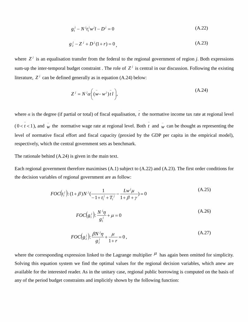
011 =−− jjjjj DlwtNg (A.22)

0)1(2 =++− rDZg jjj, (A.23)

where jZ is an equalisation transfer from the federal to the regional government of region j. Both expressions

sum-up the inter-temporal budget constraint . The role of jZ is central in our discussion. Following the existing

literature, jZ can be defined generally as in equation (A.24) below:

−=

−−

ltwwNZ jjj )(α , (A.24)

where α is the degree (if partial or total) of fiscal equalisation, −

t the normative income tax rate at regional level

( 10 <<−

t ), and −

w the normative wage rate at regional level. Both −

t and −

w can be thought as representing the

level of normative fiscal effort and fiscal capacity (proxied by the GDP per capita in the empirical model),

respectively, which the central government sets as benchmark.

The rationale behind (A.24) is given in the main text.

Each regional government therefore maximises (A.1) subject to (A.22) and (A.23). The first order conditions for

the decision variables of regional government are as follow:

( ) 0)11

1()1(: =++

−++−

+gb

µbj

jl

jl

jjl

LwTt

NtFOC (A.25)

( ) 0:1

1 =+ µηj

jj

gNgFOC

(A.26)

( ) 01

:2

2 =+

+rg

NgFOC j

jj µηb ,

(A.27)

where the corresponding expression linked to the Lagrange multiplier µ has again been omitted for simplicity.

Solving this equation system we find the optimal values for the regional decision variables, which anew are

available for the interested reader. As in the unitary case, regional public borrowing is computed on the basis of

any of the period budget constraints and implicitly shown by the following function:

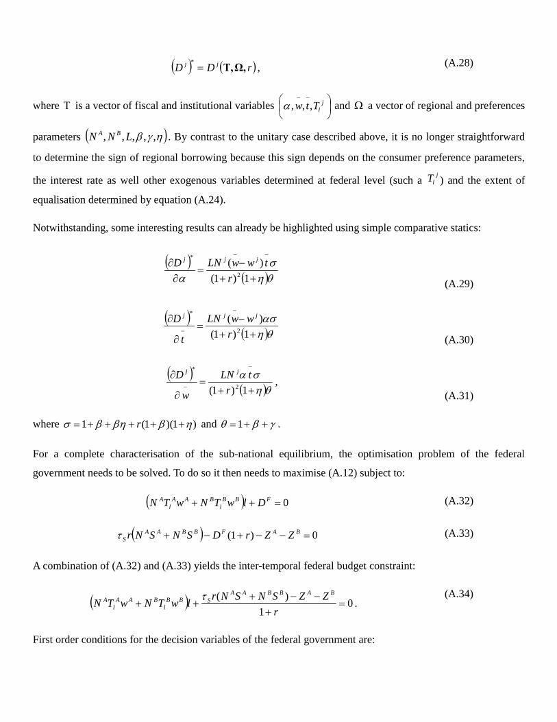
( ) ( )rDD jj Ω,Τ,=* , (A.28)

where Τ is a vector of fiscal and institutional variables

−−

jlTtw ,,,α and Ω a vector of regional and preferences

parameters ( )ηgb ,,,,, LNN BA . By contrast to the unitary case described above, it is no longer straightforward

to determine the sign of regional borrowing because this sign depends on the consumer preference parameters,

the interest rate as well other exogenous variables determined at federal level (such a jlT ) and the extent of

equalisation determined by equation (A.24).

Notwithstanding, some interesting results can already be highlighted using simple comparative statics:

( )( )θη

σα ++

−=

∂∂

−−

1)1()(

2

*

rtwwLND jjj

(A.29)

( )( )θη

ασ++

−=

∂

∂−

− 1)1()(

2

*

rwwLN

t

D jjj

(A.30)

( )( )θη

σα++

=∂

∂−

− 1)1( 2

*

rtLN

w

D jj

,

(A.31)

where )1)(1(1 ηbbηbσ +++++= r and gbθ ++=1 .

For a complete characterisation of the sub-national equilibrium, the optimisation problem of the federal

government needs to be solved. To do so it then needs to maximise (A.12) subject to:

( ) 0=++ FBBl

BAAl

A DlwTNwTN (A.32)

( ) 0)1( =−−+−+ BAFBBAAS ZZrDSNSNrτ (A.33)

A combination of (A.32) and (A.33) yields the inter-temporal federal budget constraint:

( ) 01

)(=

+−−+

++r

ZZSNSNrlwTNwTNBABBAA

SBBl

BAAl

A τ . (A.34)

First order conditions for the decision variables of the federal government are:

( ) ( )( ) 0)1

))1)(1((1

1: =+

+++−+

++−+

rrrwLN

TtNTFOC S

AA

Al

Al

AA

l θbτbµδb

(A.35)

( ) ( )( ) 0)1

))1)(1((1

)1(1: =+

+++−+

++−−+

rrrwLN

TtNTFOC S

BB

Bl

Bl

BB

l θbτbµδb

(A.36)

( ) ,0)1(1

)1()1(

))1()1((: =

−+

−+−

+++−+++−

S

BABl

Bl

BBAl

Al

AA

S rNN

rTtwNTtwNLrFOC

τδ

θµbτ

(A.37)

where that corresponding to the auxiliary variable of the langrangian has again been omitted. Equation system

(A.35)-(A.37) and the federal budget constraint are then solved for the endogenous variables, which are

available upon request. Federal public borrowing ( )*FD is determined using these optimal values in any of the

budget constraints:

( )( )

( )r

twwNwwNLD

BBAA

F

+

+

−+−

−=

−−−

1

1)()(*

θ

bα

(A.38)

References

Ahmad, E., Searle, B., 2005. On the Implementation of Transfers to Sub-national Governments. IMF Working Paper, 05-130.

Argimon, I., Hernandez de Cos, P., 2012. Fiscal Rules and Federalism as Determinants of Budget Performance. An Empirical Investigation for the Spanish Case. Public Finance Review. 40 (1), 30-65.

Alt, J.E., Lowry, R. C., 1994. Divided government, fiscal institutions and budget deficits: evidence from the States. American Political Science Review. 88(4), 811-828.

Balassone, F., Zotteri, S., 2002. Fiscal rules for sub-national governments: what lessons for EMU countries?, Paper prepared for the Conference on “Rules-Based Macroeconomic Policies in Emerging Market Economies” IMF and the World Bank Conference, Oaxaca – Mexico.

Baretti C., Huber B., and Lichtblau K. (2002). A tax on tax revenues: The incentive effects of equalizing transfers: Evidence from Germany. International Tax and Public Finance 9 (6), 631-649.

Barrios, S. Martinez-Lopez, D. (2014). Fiscal equalisation schemes and sub-central government borrowing. Working Paper #1401. Universidade de Vigo, GEN - Governance and Economics research Network.

Barrios, S., Strobl, E., 2009. The dynamics of regional inequalities. Regional Science and Urban Economics. 39(5), 575-591.

Barrios, S., Rizza, P., 2010. Unexpected changes in tax revenues and the stabilisation function of fiscal policy. Evidence for EU. European Economy - Economic Papers 404. Directorate General Economic and Monetary Affairs, European Commission.

Baskaran, T. (2012). Soft budget constraints and strategic interactions in subnational borrowing: Evidence from the German States, 1975-2005. Journal of Urban Economics 71 (1), 114.127. Bird, R., Tassonyi, A., 2003. Constraining Sub-national Fiscal Behaviour in Canada: Different Approaches", Similar results?, in: Rodden, J. A., G. S. Eskeland and J. Litvack, (Eds.), Fiscal decentralization and the challenge of hard budget constraints, MIT Press, Cambridge.

Blöchliger, H., Charbit, C., 2008. Fiscal equalization. OECD Economic Studies No. 44, 2008/1.

Blundell, R., Bond, S., 1998. Initial conditions and moment restrictions in dynamic panel data models. Journal of Econometrics. 87(1), 115-143.

Boadway, R., Flatters, F., 1982. Efficiency and Equalization Payments in a Federal System of Government: A Synthesis andExtension of Recent Results. Canadian Journal of Economics, 15 (4), 613-633.

Boadway, R. and A. Shah (2007). Intergovernmental fiscal transfers: principles and practice. Number 7171. Washington, D.C.: The World Bank Publications. Bohn, H., 1998. The Behaviour of U.S. Public Debt and Deficits. Quarterly Journal of Economics. 113, 949-963.

Buchanan, J. M. (1950). Federalism and fiscal equity. The American Economic Review, 583-599. Buettner, T., 2006. The incentive effects of fiscal equalization transfers on tax policy. Journal of Public Economics. 90(3), 477-497.

Buettner T., 2009. The contribution of equalization transfers to fiscal adjustments: Empirical results for German municipalities and a US-German comparison. Journal of Comparative Economics 37(3), 477-497.

Celasun, O. Kang, J. S., 2006. On the properties of Various Estimators for Fiscal Reaction Functions. IMF Working Paper 06/182, International Monetary Fund, Washington D.C.

Dahlby, B., 2008. The Canadian federal-provincial equalization system. CESifo DICE Report 1/2008.

Duval, R., Elmeskov, J., 2006. The Effects of EMU on Structural Reforms in Labour and Product Markets. ECB Working Paper No. 596.

Egger, P., Koethenbuerger, M. Smart, M., 2010. Do fiscal transfers alleviate business tax competition? Evidence from Germany. Journal of Public Economics. 94(3), 235-246.

European Commission, 2012. Public Finances Report in EMU 2012. Directorate General for Economic and Financial Affairs, Brussels.

Eyraud, L. and L. Lusinyan, (2013), Vertical Fiscal Imbalances and Fiscal Performance in Advanced Economies, Journal of Monetary Economics, forthcoming.

Fatás, A., Mihov, I., 2003. The case for restricting fiscal policy discretion. Quarterly Journal of Economics. 118(4), 1419-1447.

Federal Ministry of Finance (Germany), 2009. Federation/Länder financial relations on the basis of constitutional financial provisions. Berlin.

Foremny, D., von Hagen, J., 2012. Fiscal federalism in times of crisis. CEPR Discussion Paper #9154.

Goodspeed, T. J. (2002). Bailouts in a federation. International Tax and Public Finance 9(4), 409.421.

Guillemette, Y., 2010. Fiscal-Consolidation Strategies for Canadian Governments. OECD Economics Dept. Working Paper 818, OECD, Paris.

Heppke-Falk, K. H., Wolff, G. B., 2008. Moral Hazard and Bail-Out in Fiscal Federations: Evidence for the German Länder. Kyklos. 61(3), 425-446.

Hierro, L. A., Atienza, P. and Patiño, D. (2010). El efecto redistributivo de las transferencias en la financiación regional, Revista de Economía Aplicada, 53, 99-129. English version as wp: "Inequality and Progressiveness in the Distribution of Revenues of the States in Federal Countries: A Comparative Study," International Center for Public Policy Working Paper Series, Georgia State University.

Hodrick, R.J., Prescott, E. C., 1997. Postwar U.S. Business Cycles: An Empirical Investigation. Journal of Money, Credit and Banking. 29(1), 1-16.

Kiviet, J.F., 1995. On Bias, Inconsistency and Efficiency of Various Estimators in Dynamic Panel Data Models. Journal of Econometrics. 68, 53-78.

Lago, S., 2005. Evolving Federations and Regional Public Deficits: Testing the Bailout Hypothesis in the Spanish Case. Environment and Planning C: Government and Policy. 23 (3), 437-454.

Liu, Y., 2014. Does competition for capital discipline governments? The role of fiscal equalization. International Tax and Public Finance, 21(3), 345-374.

Martínez-López, D., 2005. On states’ behavior with equalization grants. Hacienda Pública Española, 174(3), 43-54.

Molina-Parra, A. and Martinez-Lopez, D. (2015). Do federal deficits motivate regional fiscal (im)balances? Evidence from the Spanish case. Mimeo. Forthcoming as working paper in the Governance and Economics research Network (GEN).

OECD, 2009. Explaining the sub-national tax-grants balance in OECD countries. OECD Network on Fiscal Relations across Levels of Government, Working Paper no. 11.

OECD, 2013. Fiscal Federalism 2014: Making Decentralisation Work, OECD Publishing.

Padovano, F. 2014. Distribution of transfers and soft budget spending behaviors: evidence from Italian regions. Public Choice, forthcoming.

Pitlik, H., F. Schneider and H. Strotmann, 2006. Legislative Malapportionment and the Politicization of Germany’s Intergovernmental Transfer System”, Public Finance Review, 34, 637-662.

Potrafke, N. and Reischmann, M. 2012. Fiscal Equalization Schemes and Fiscal Sustainability. CESifo Working Paper Series No. 3948.

Ravn, M. O., Uhlig, H., 2002. On Adjusting the Hodrick-Prescott Filter for the Frequency of Observations. Review of Economics and Statistics. 84 (2), 371-376.

Rodden, J. A., G. S. Eskeland and J. Litvack, (2003), "Fiscal decentralization and the challenge of Hard Budget constraints", MIT Press, Cambridge.

Rodden, J.A., 2006. Hamilton´s Paradox. The Promise and Peril of Fiscal Federalism. MIT Press, Cambridge.

Ruiz-Huerta, J. Herrero, A., 2008. Fiscal equalization in Spain, in: Bosch, N., Duran, J. M. (2008): Fiscal federalism and political decentralization. Edward Elgar.

Schakel, A.H., 2011. Congruence Between Regional and National Elections. Comparative Political Studies. XX(X), 1–32.

Schuknecht, L., Von Hagen, J., Wolswijk, G.., 2009. Government risk premiums in the bond market: EMU and Canada. European Journal of Political Economy. 25(3), 371-384.

Simon-Cosano, P., S. Lago-Peñas and A. Vaquero (2013). On the Political Determinants of Intergovernmental Grants in Decentralized Countries: The Case of Spain. Publius, 43 (2), 1-22.

Smart, M., 1998. Taxation and Deadweight Loss in a System of Intergovernmental Transfers. Canadian Journal of Economics, 31(1), 189-206.

Sutherland, D., Price, R., Joumard, I., 2005. Sub-Central Government Fiscal rules. OECD Economic Studies 41, 2005/2.

Ter-Minassian, T., Fedelino, A., 2010. Impact of the global crisis on sub-national governments' finance. Bank of Italy Occasional Paper.

Vallés, J., Zárate, A., 2004. Un análisis de las restricciones institucionales para el control de la deuda regional en perspectiva histórica. Moneda y Crédito. 219, 143-175.

Velasco, A., 2000. Debts and deficits with fragmented fiscal policymaking, Journal of Public Economics 76, 105-125.

Von Hagen, J., Bordignon, M., Dahlberg, M., Grewal, B. S., Peterson, P., Seitz, H., 2000. Sub-national Government Bailouts in OECD Countries: Four Case Studies. IDB Working Paper No. 126.

Von Hagen, J., Eichengreen, M., 1996. Federalism, fiscal restraints and European Monetary Union. American Economic Review. 86 (2), 134-138.

Zabalza, A., 2003. A general framework for the analysis of fiscal equalisation systems. Spanish Economic Review. 5, 205-232.

Zipfel, F., 2011. German finances: federal level masks importance of Länders. Deutsche Bank Research.