FIRST YEAR PHYSICS LABORATORY (P141) MANUAL

LIST OF EXPERIMENTS 2015-16

1. Measurement of ‘g’ using compound pendulum.

2. Measurement of Moment of inertia of different bodies and proof of parallel

axis theorem.

3. Measurement of Young’s modulus by bending of beam method.

4. Study of Soft massive spring.

5. Measurement of Specific Heat of Graphite.

6. Measurement of Electrical Equivalent of Heat.

7. Measurement of Thermal conductivity of a bad conductor.

8. Measurement of Co-efficient of Viscosity by dropping ball method.

9. Measurement of Surface Tension using capillary rise method.

1

Measurement of acceleration due to gravity (g) by a compound pendulum

Aim: (i) To determine the acceleration due to gravity (g) by means of a compound pendulum.

(ii) To determine radius of gyration about an axis through the center of gravity for the

compound pendulum.

Apparatus and Accessories: (i) A bar pendulum, (ii) a knife–edge with a platform, (iii) a sprit

level, (iv) a precision stop watch, (v) a meter scale and (vi) a telescope.

Theory:

A simple pendulum consists of a small body called a “bob” (usually a sphere) attached to

the end of a string the length of which is great compared with the dimensions of the bob and the

mass of which is negligible in comparison with that of the bob. Under these conditions the mass

of the bob may be regarded as concentrated at its center of gravity, and the length of the

pendulum is the distance of this point from the axis of suspension. When the dimensions of the

suspended body are not negligible in comparison with the distance from the axis of suspension to

the center of gravity, the pendulum is called a compound, or physical, pendulum. A rigid body

mounted upon a horizontal axis so as to vibrate under the force of gravity is a compound

pendulum.

In Fig.1 a body of irregular shape is pivoted about a horizontal frictionless axis through P and is

displaced from its equilibrium position by an angle θ. In the equilibrium position the center of

gravity G of the body is vertically below P. The distance GP is l and the mass of the body is m.

The restoring torque for an angular displacement θ is

τ = - mg l sinθ …(1)

For small amplitudes (θ ≈ 0),

� ������ � ���, …(2)

where I is the moment of inertia of the body through the axis P.

Eq. (2) represents a simple harmonic motion and hence the time

period of oscillation is given by

� 2�� ���� …(3)

Now � � �� ���, where IG is the moment of inertia of the

body about an axis parallel with axis of oscillation and passing

through the center of gravity G.

IG = mK2 …(4)

where K is the radius of gyration about the axis passing through

G. Thus,

G

P

l

Fig. 1

θ

O

L

2

� 2������������ � 2����� ��� …(5)

The time period of a simple pendulum of length L, is given by

� 2� ��� …(6)

Comparing with Eq. (5) we get

� � � � ��� …(7)

This is the length of “equivalent simple pendulum”. If all the mass of the body were concentrated

at a point O (See Fig.1) such that � � !�� � � , we would have a simple pendulum with the same

time period. The point O is called the ‘Centre of Oscillation’. Now from Eq. (7)

�� � �� � "� � 0 ...(8)

i.e. a quadratic equation in l. Equation 6 has two roots l1 and l2 such that

�$ � �� � �

and �$�� � "� …(9)

Thus both �$ and �� are positive. This means that on one side of C.G there are two positions of

the centre of suspension about which the time periods are the same. Similarly, there will be a pair

of positions of the centre of suspension on the other side of the C.G about which the time periods

will be the same. Thus there are four positions of the centers of suspension, two on either side of

the C.G, about which the time periods of the pendulum would be the same. The distance between

two such positions of the centers of suspension, asymmetrically located on either side of C.G, is

the length L of the simple equivalent pendulum. Thus, if the body was supported on a parallel

axis through the point O (see Fig. 1), it would oscillate with the same time period T as when

supported at P. Now it is evident that on either side of G, there are infinite numbers of such pair

of points satisfying Eq. (9). If the body is supported by an axis through G, the time period of

oscillation would be infinite. From any other axis in the body the time period is given by Eq. (5).

From Eq.(6) and (9), the value of g and K are given by

� 4�� �)� …(10)

" � *�$�� …(11)

By determining L, �$ and �� graphically for a particular value of T, the acceleration due to

gravity g at that place and the radius of gyration K of the compound pendulum can be

determined.

3

Description:

The bar pendulum consists of a metallic bar of about one meter long. A series of circular holes

each of approximately 5 mm in diameter are made along the length of the bar. The bar is

suspended from a horizontal knife-edge passing through any of the holes (Fig. 2). The knife-

edge, in turn, is fixed in a platform provided with the screws. By adjusting the rear screw the

platform can be made horizontal.

Procedure:

(i) Suspend the bar using the knife edge of the hook through a hole nearest to one end of the bar.

With the bar at rest, focus a telescope so that the vertical cross-wire of the telescope is coincident

with the vertical mark on the bar.

(ii) Allow the bar to oscillate in a vertical plane with small amplitude (within 40 of arc).

(iii) Note the time for 20 oscillations by a precision stop-watch by observing the transits of the

vertical line on the bar through the telescope. Make this observation three times and find the

mean time t for 20 oscillations. Determine the time period T.

(iv) Measure the distance d of the axis of the suspension, i.e. the hole from one of the edges of

the bar by a meter scale.

(v) Repeat operation (i) to (iv) for the other holes till C.G of the bar is approached where the time

period becomes very large.

Fig. 2 Fig. 3

4

(vi) Invert the bar and repeat operations (i) to (v) for each hole starting from the extreme top.

(vii) Draw a graph with the distance d of the holes as abscissa and the time period T as ordinate.

The nature of graph will be as shown in Fig. 3.

Draw the horizontal line ABCDE parallel to the X-axis. Here A, B, D and E represent the point

of intersections of the line with the curves. Note that the curves are symmetrical about a vertical

line which meets the X-axis at the point G, which gives the position of the C.G of the bar. This

vertical line intersects with the line ABCDE at C. Determine the length AD and BE and find the

length L of the equivalent simple pendulum from � � +,�-.� � �/� .

Find also the time period T corresponding to the line ABCDE and then compute the value of g.

Draw several horizontal lines parallel to X-axis and adopting the above procedure find the value

of g for each horizontal line. Calculate the mean value of g. Alternatively, for each horizontal

line obtain the values of L and T and draw a graph with T2 as abscissa and L as ordinate. The

graph would be a straight line. By taking a convenient point on the graph, g may be calculated.

Similarly, to calculate the value of K, determine the length AC, BC or CD, CE of the line

ABCDE and compute √12ΧB2 or √24Χ25. Repeat the procedure for each horizontal line. Find

the mean of all K.

Observations:

Table 1-Data for the T versus d graph

Serial no of

holes from one

end

Distance d of

the hole from

one end (cm)

Time for 20

oscillations (sec)

Mean time t for

20 oscillations

(sec)

Time period

T = t/20 (sec)

One

side of

C.G

1 ….. ….

….

….

….. …..

2 ….. …..

……

….

…. ……

3 …… ….

.….

……

….. ……..

Other

side of

C.G

1 ….. ….

….

….

….. …..

2 ….. …..

……

……

…. ……

3 …… ……

…….

……

….. ……..

5

TABLE 2- The value of 6 and K from T vs. d graph

No. of obs.

�

(cm)

T

(sec) � 4�� � �

(cm/sec2)

Mean‘’

(cm/sec2)

K

(cm)

Mean ‘K’

(cm)

1. ABCDE

2.

3.

(AD+BE)/2

..

..

..

..

..

..

..

..

√12ΧB2 or √24Χ25 ..

..

Computation of proportional error:

We have from Eq. (10) � 4�� 7�//�97 :�;9� …(12)

Since L = Lx/2 (Lx= AD+BE) and T = t/20, therefore, we can calculate the maximum proportional

error in the measurement of g as follows

<�� � �=<�/�/ >� � =2 <�� >� … (13)

?�@ = the value of the smallest division of the meter scale ?A = the value of the smallest division of the stop-watch

Precautions and Discussions:

(i) Ensure that the pendulum oscillates in a vertical plane and that there is no

rotational motion of the pendulum.

(ii) The amplitude of oscillation should remain within 40 of arc.

(iii) Use a precision stop-watch and note the time accurately as far as possible.

(iv) Make sure that there is no air current in the vicinity of the pendulum.

References:

1. Fundamentals of Physics: Resnick & Halliday

2. Practical physics: R.K. Shukla, Anchal Srivatsava, New Age International (P) Ltd, New Delhi

3. Eric J. Irons, American Journal of Physics, Vol. 15, Issue 5, pp.426 (1947)

Moment of Inertia of different bodies and parallel axis theorem

Aim: 1) Study moment of inertia of different bodies and 2) prove the parallel axis theorem

(Steiner’s theorem)

Objectives of the experiment (Part 1)

� Determining the moments of inertia of rotationally symmetric bodies from their period of

oscillation on a torsion axle.

� Comparing the periods of oscillation of two bodies having different masses, but the same

moment of inertia.

� Comparing the periods of oscillation of hollow bodies and solid bodies having the same

mass and the same dimensions.

� Comparing the periods of oscillation of two bodies having the same mass and the same

body shape, but different dimensions.

Thoery: The moment of inertia is a measure of the resistance of a body against a change of its

rotational motion and it depends on the distribution of its mass relative to the axis of rotation. For

a calculation of the moment of inertia J, the body is subdivided into sufficiently small mass

elements ∆mi with distances ri from the axis of rotation and a sum is taken over all mass

elements:

� � ∑ ∆��. ��� (1)

For bodies with a continuous mass distribution, the sum can be converted into an integral.

If, in addition, the mass distribution is homogeneous, the integral reads

� � . �� �� �� (2)

The calculation of the integral is simplified when rotationally symmetric bodies are

considered which rotate around their axis of symmetry. The simplest case is that of a hollow

cylinder with radius R. As all mass elements have the distance R from the axis of rotation, the

moment of inertia of the hollow cylinder is

��� � . � (3)

In the case of a solid cylinder with equal mass M and equal radius R, Eq. (II) leads to the

formula

��� � . 1� � �. 2�. �. �. ������� � �. �. ���

And the result is

��� � � . � (4)

Fig. 1: Calculation of the moments of inertia of a hollow cylinder, a solid cylinder and a sphere

That means, the moment of inertia of a solid cylinder is smaller than that of the hollow

cylinder as the distances of the mass elements from the axis of rotation are between 0 and R.

An even smaller value is expected for the moment of inertia of a solid sphere with radius

R (see Fig. 1). In this case, Eq. (2) leads to the formula

��� � . 1� � �. 2�. �. 2. �� �.�� ������� � 4�3 �#

and the result is ��� � % . . � (5)

Thus, apart from the mass M and the radius R of the bodies under consideration a

dimensionless factor enters the calculation of the moment of inertia, which depends on the shape

of the respective body.

The moment of inertia is determined from the period of oscillation of a torsion axle, on

which the test body is fixed and which is connected elastically to the stand via a helical spring.

The system is excited to perform harmonic oscillations. If the restoring torque D is known, the

moment of inertia of the test body is calculated from the period of oscillation T according to

� � &. ' ()*

(6)

Setup and carrying out the experiment

The experimental setup is illustrated in Fig 2.

– Put the sphere on the torsion axle, and mark the equilibrium position on the table.

– Rotate the sphere to the right by 180° and release it.

– Start the time measurement as soon as the sphere passes through the equilibrium position and

stop the measurement after five oscillations (5T).

– Calculate the period of oscillation T.

– Replace the sphere with the disk, and repeat the measurement.

– Replace the disk with the supporting plate.

– Repeat the measurement with the solid cylinder and then with the hollow cylinder.

– Finally carry out the measurement with the empty supporting plate.

Fig.2: Setup for measuring time period

Data

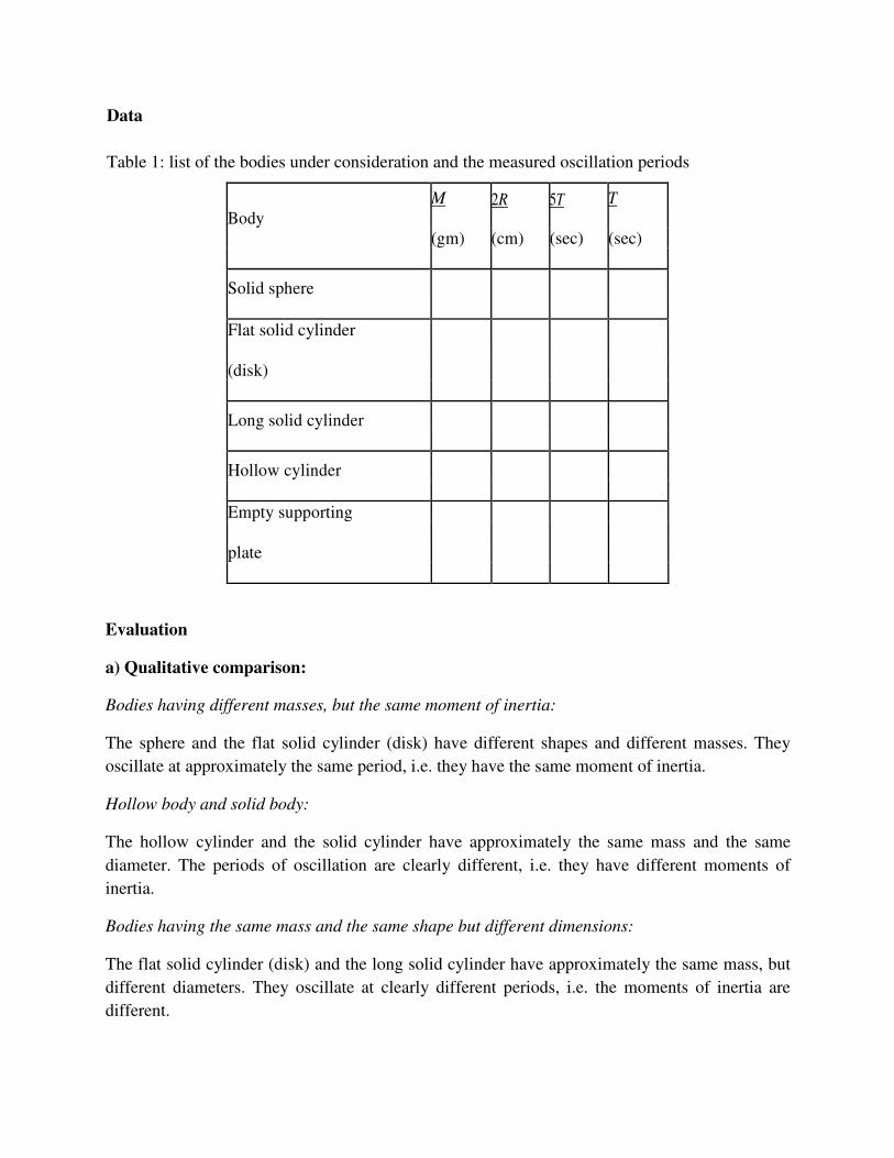
Table 1: list of the bodies under consideration and the measured oscillation periods

Body

M 2R 5T T

(gm) (cm) (sec) (sec)

Solid sphere

Flat solid cylinder

(disk)

Long solid cylinder

Hollow cylinder

Empty supporting

plate

Evaluation

a) Qualitative comparison:

Bodies having different masses, but the same moment of inertia:

The sphere and the flat solid cylinder (disk) have different shapes and different masses. They

oscillate at approximately the same period, i.e. they have the same moment of inertia.

Hollow body and solid body:

The hollow cylinder and the solid cylinder have approximately the same mass and the same

diameter. The periods of oscillation are clearly different, i.e. they have different moments of

inertia.

Bodies having the same mass and the same shape but different dimensions:

The flat solid cylinder (disk) and the long solid cylinder have approximately the same mass, but

different diameters. They oscillate at clearly different periods, i.e. the moments of inertia are

different.

b) Quantitative comparison:

With Eq. (6), the moments of inertia J can be calculated from the periods T listed in Table 1.

The restoring torque D of the torsion axle required for the calculation equal to D=0.023

Newton.meter/rad

Calculate dimensionless factors of Eqs. (3), (4) and (5) and compare with the values calculated

from the measuring data.

Body Moment of inertia J

(gm.cm2)

Measurement

(J/MR2)

Thoery

(J/MR2)

Solid sphere

disk

Solid cylinder

Hallow cylinder

Part 2: Verification of Steiner’s theorem (Parallel axis theorem)

Theory:The moment of inertia of an arbitrary rigid body whose mass element ∆mi have the

distances ri from the axis of rotation A is�+ � ∑ ∆��. ��� (1)

If the axis of rotation does not pass through the centre of mass of the body, application of Eq.(1)

leads to an involved calculation. Often it is easier to calculate the moment of inertia Js with

respect to the axis S, which is parallel to the axis of rotation and passes through the centre of

mass of the body.

For deriving the relation between JA and Js, the plane perpendicular to the axis of rotation where

the respective mass element ∆mi and the vector sipoints from the centre-of –mass axis to the

element. Thus

�� � , - .� (2)

And the squares of the distances in Eq.(1) are

�� � /,� - .�0 � , - 2. ,. .� - .� (3)

Therefore the sum in Eq.(1) can be split into three terms:

�+ � 12∆

���3 . , - 2. 12∆��..�

�3 . , - 2∆��..��

In the first summand,

∑ ∆��� � is the total mass of the body. In the last summand,∑ ∆��� . s5 � J7 is the moment of

inertia of the body with respect to the centre-of-mass axis. In the middle summand, ∑ ∆��� . .� �0because the vectors si start from the axis through the centre of mass.

Thus Steiner’s theorem follows from Eq(4)

�+ � . , - �� (5)

This theorem will be verified in the experiment with a flat circular disk as an example. Its

moment of inertia JA with respect to an axis of rotation at a distance a from the axis of symmetry

is obtained from the period of oscillation T of a torsion axle to which the circular disk is

attached. We have

� � &. ' ()*

(6)

D: restoring torque of the torsion axle

Fig 1. Schematic illustration referring to the derivation of Steiner’s theorem

Procedure:

The experimental setup is illustrated in Fig 2.

– Fix the centre of the circular disk to the torsion axle and mark the equilibrium position on the

table.

– Rotate the circular disk by 180° from the equilibrium position and release it.

– Start the time measurement as soon as the circular disk passes through the equilibrium position

and stop the measurement after five oscillations.

– Repeat the measurement four times alternately deflecting the disk to the left and to the right.

– Calculate the period of oscillation T from the mean value of the five measurements.

– Mount the circular disk on the torsion axle so that its centre is at a distance of 2 cm from the

axle, and, if necessary, mark the equilibrium position anew.

– Measure the time of five oscillations five times alternately deflecting the disk to the right and

to the left.

– Calculate the period of oscillation T.

– Repeat the measurement for other distances a from the axis of symmetry.

Fig.2 Setup for confirmation of Steiner’s theorem

Observations

Mass of the disk: M = --- g Radius of the disk: R = ---cm

Table 1: measured time of five oscillations (measured five times) for various distances a between

the axis of rotation and the axis of symmetry and oscillation periods T calculated from the mean

value of the measured values

a(cm) Measurement of time period for 5 oscillations T (sec)

0

2

4

6

8

10

12

14

16

Evaluation

With the aid of Eq. (6), the moment of inertia JA can be calculated from the values of the period

of oscillation listed in Table 1. The restoring torque D required for the calculation is equal

to D=0.023 Newton.meter

Calculate the moment of inertia at various distances and plot JA versus a2and interpret results.

1

TO DETERMINE YOUNG’S MODULUS OF ELASTICITY OF THE MATERIAL OF A

BAR BY THE METHOD OF FLEXURE

Aim: To determine the Young’s modulus of elasticity of the given material.

Apparatus: meter scale, screw gauge, spherometer and slide caliper

Theory: If a light bar of breadth b and depth d is placed horizontally on two Knife-edges

separated by a distance L, and a load of mass m, applied at the mid-point of the bar, produces a

depression l of the bar, then Young’s modulus Y of the material of the bar is given by

� � ������� (1)

whereg is the acceleration due to gravity. This is the working formula of the experiment, and is

valid so long as the slope of the bar at any point with respect to the unstrained position is much

less than unity. Here Y is determined by measuring the quantities b, d, Land the mean depression

lcorresponding to a load m. If b, d, L and l are measured in cm, m in gm, g is expressed in

cm/sec2, and then Y is obtained in dyne/cm

2.

Procedure:

(i) Measure the length of the given bar with a meter scale and place the centre of the bar at

the middle point of the two supports fixed to the table.

(ii) Place rectangular hook cum hanger at the centre of the scale. Place the spherometer such

that screw of spherometer is on top of the rectangular hook cum hanger.

(iii) Make the electrical connections as shown in the figure(1) by connecting power supply,

spherometer and galvanometer.

(iv) Switch on the power supply, adjust the circular scale such that screw of spherometer(S)

touches rectangular hook, indicating deflection in the Galvanometer (G)

(v) Take the initial reading on the spherometer.

(vi) Hang a weight to the hook and then you notice that galvanometer reading come back to

zero (why?). Again adjust the spherometer such that screw touches the hook and

galvanometer deflects. Take the depression of the bar reading corresponding the weight

hanged.

(vii) Continue the same procedure for all the weights. Avoid back lash error while using

spherometer.

(viii) Repeat the experiment once again with all the weights

2

Figure 1: Schematic diagram of electrical connections

(ix) Determine the vernier constant of the slide callipers and measure with it the breadth b of

the bar at three different places. Calculate the mean breadth of the bar. Note the zero

error, if any, of the slide callipers and find the correct value of b.

(x) Determine the least count of the screw gauge and measure depth d of the bar at a number

of places along the length of the bar. Find the mean value. Note the zero error, if any of

the screw gauge and obtain the correct value of d.

(xi) Draw a graph with the load m in gm along the X-axis and the corresponding depression l

in cm along the Y-axis and determine the value of Y.

Experimental Results:

Table-1

Least count of spherometer

Pitch of the screw p (cm) No. of divisions n on the

circular scale

Least count = p/n (cm)

…….

…………

……………

+ -

G

S

3

Table-2 :Load-depression data for chosen length

Distance between the knife-edges L = ……cm

No.

of

obs.

Load

in

(kg)

spherometer reading for

Increasing load (cm)-

first measurement

Spherometer reading

for increasing load

(cm)- second

measurement

Mean

reading

(cm)

Depression

l(cm)

Main

scale

Circular Total Main

scale

Circular Total

1

2

3

..

..

..

..

..

..

..

..

..

..

..

..

..

..

..

..

..

..

..

..

..

..

..

..

..

..

..

..

..

..

..

..

….(a)

…..(b)

…….(c)

…

…

0

(b)-(a)

(c)-(a)

…

…

Table-3

Vernier Constant (v.c.) of the slide calipers

….. Divisions of the vernier scale = ………… divisions of the main scale.

Value of l smallest main

scale division (l1)

Value of 1vernier division

(�� � � ��) (cm)

Vernier constant

v.c. = (�� � ��� (cm)

…………. ……………… …………………..

Table-4: Measurement of breadth (b) of the bar by slide calipers

No.

of

obs.

Readings (cm) of

the

Total

readingb(cm)

Mean b

(cm)

Zero

error(cm)

Correct b

(cm)

Main

scale

Vernier

Table-5: Least count (L.C.) of the screw gauge

Pitch of the screw p (cm) No. of divisions n on the

circular scale

Least count = p/n (cm)

…….

…………

……………

4

Table–6: Measurement of depth (d) of the bar by the screw gauge

No.

of

obs.

Readings (cm) of

the

Total

reading

d (cm)

Mean d

(cm)

Zero error

(cm)

Correct d

(cm)

Main

scale

Vernier

1

2

3

…

…

…

…

…

…

…

…

…

…

…

…

Discussions:

Even though entire scale or bar deforms by applying stress to given bar or scale, length Lin

� � ������� correspond to the portion between two knife edges but not the total length of the

given bar or meter scale. Why? Refer to supporting material.

Computation of proportional error: We have� � ������� . The quantities L, b, d, and �are

measured in this experiment. The maximum proportional error in Y due to errors in the

measurement of L, b, d, and �is given by

��� � ��3��� �� � ���� �

� � �3��� �� � ���� �

�

Precautions:(i) In the expression for Y, both the length L between the knife-edges and the depth

d of the bar occur in powers of three. But as d is much smaller than L, much care should be taken

to measure to minimize the proportional error in Y.

(ii) Care should be taken to make the beam horizontal and to load the bar at its mid-point.

(iii) Try to avoid parallax and back-lash errors during measurements.

Objectives: 1) To determine the spring constant and the mass correction factor for the given soft massive

spring by static (equilibrium extension) method.

2) To determine the spring constant and the mass correction factor for the given soft massive

spring by dynamic (spring mass oscillations) method.

3) To determine the frequency of oscillations of the spring with one end fixed and the other

end free i.e. zero mass attached.

4) To study the longitudinal stationary waves and to determine the fundamental frequency of

oscillations of the spring with both the ends fixed.

Apparatus: 1) A soft massive spring

2) A long and heavy retort stand with a clamp at the top end

3) A set of calibrated mass with hooks (including fractional mass)

4) A function generator with its connecting cord

5) A dual output power amplifier with the connecting cords

6) A mechanical vibrator mounted on the retort stand

7) A digital multimeter (to be used as frequency counter)

8) A digital stopwatch

9) A measuring tape (3.0 m)

10) Two measuring scales (1.0 m and 0.6 m)

11) A tissue paper

Introduction: A spring is a flexible elastic device, which stores potential energy on account of straining of

the bonds between the atoms of the elastic material of the spring. A variety of springs are

available which are designed and fabricated to suit the various mechanical systems. Most

common types of springs are compression springs, extension springs and torsion spring.

There are some special types of springs like leaf spring, V-spring, spiral spring etc. The coil

or helical type of springs can have cylindrical or conical shape.

Robert Hooke, a 17th

century physicist studied the behavior of springs under different loads.

He established an equation, which is now known as Hooke’s law of elasticity. This law states

that the amount by which a material body is deformed (the strain) is linearly proportional to

the force causing the deformation (the stress). Thus, when applied to a spring, Hooke’s law

implies that the restoring force is linearly proportional to the equilibrium extension. F = −

K x, where F is the restoring force exerted by the spring, x is the equilibrium extension and K

is called the spring constant. (The negative sign indicates that the force F is opposite in

direction to the extension x. Hence also the term ‘restoring force’.) For this equation to be

valid, x needs to be below the elastic limit of the spring. If x is more than the elastic limit, the

spring will exhibit ‘plastic behavior’, where in the atomic bonds in the material of the spring

get broken or rearranged and the spring does not return to its original state. It may be noted

that the potential energy U stored in a spring is given by U = ½ K x2.

Depending on the value of the spring constant, a spring can be called as a soft or hard spring.

A spring can be called mass-less or massive, depending on the mass, which needs to be

SOFT MASSIVE SPRING

attached to get a considerable extension in the spring. Sometimes springs are also categorized

by the ratio of spring constant to the mass of the spring (K/ms). A soft massive spring has a

low spring constant and its mass can not be neglected.

In the determination of the spring constant of a spring, we generally neglect the effect of the

mass of the spring on the equilibrium extension or the time period of oscillation of the spring

for a given mass attached. In the case of soft massive springs the mass of the spring cannot be

neglected. These types of springs have extension under their own weight and therefore need a

correction for the extension. Similarly, they oscillate without any attached mass, which

implies that the standard formula for the time period of oscillations of a spring needs

modification. People have theoretically worked out the modification and corrected the

formula for the equilibrium extension and also the time period of oscillations. Interestingly,

one finds that the mass correction factors in these two cases are not the same. In this problem,

we will experimentally study and verify the modified formulae.

An extended soft massive spring clamped at both the ends can be assumed to be a uniformly

distributed mass system. It has its own natural frequencies of oscillations (corresponding to

different normal modes) like a hollow pipe closed at both the ends. Using the method of

resonance we will excite and study different normal modes of vibrations of the spring. Here

the longitudinal stationary waves will be set up on the extended soft massive spring.

Description: In Part A, we will use the static method, where the equilibrium extension of a given spring

will be measured for different attached mass and the spring constant and the mass correction

factor will be determined. In Part B, we will use the dynamic method, where different mass

will be attached to the lower end of the spring with its upper end fixed and corresponding

time period of oscillations for such a spring-mass system will be measured. Also the

frequency of oscillations of the spring with the upper end fixed and the lower end free i.e. the

zero attached mass will be determined graphically. In Part C, we will use a mechanical

vibrator to force oscillations on the spring and excite different normal modes of vibrations of

the spring. Thus the longitudinal stationary waves will be set up on the spring. We will

measure the frequencies of excitation corresponding to different normal modes. From these,

the fundamental frequency of oscillation with both the ends fixed will be determined. We will

compare this frequency with the frequency of oscillations with one end fixed and the other

end free as determined earlier in Part B.

Theory: Part A:

Let Lo be the length of the spring when the spring is kept horizontal under no tension, m be

the mass attached to the free end of the spring, Lm be the length of the spring when the mass

is attached at its lower end, Sm be the equilibrium extension of the spring for mass m, ms be

the mass of the spring, K be the spring constant and g be the acceleration due to gravity.

Thus,

( )1omm LLS −=

Note that the tension in the spring varies along the spring from (m + ms)g at the top to mg at

the bottom.

We can write,

xgCgmmxT s −+= )()(

where, C is a constant of proportionality. C = ms/Lo and x is the distance from the top of the

given point; x varies from 0 to Lo.

We can determine the expression for Sm, by taking extension of a small element of length ∆x

and integrating over the total length of the spring.

The final expression, which we get is,

( )22

+=

K

gmmS s

m

where, (ms/2) is called the mass correction factor (static case) mcs.

Part B:

The expression for the time period of oscillations T for an ideal (mass-less) spring-mass

system is given by,

K

mT π2=

In case of the soft massive springs, we cannot neglect the mass of the spring since these

springs can oscillate without any attached mass. We thus need to modify the above

expression for T. This can be done using the principle of conservation of energy,

i.e. Potential Energy + Kinetic Energy = constant.

The modified expression, which we get is,

( )33

2K

mm

T

s

+

= π

where (ms/3) is again the mass correction factor (dynamic case) mcd. Note that the mass

correction factors in Part A and Part B are different.

The corresponding frequency of oscillations f ' is given by,

Tf

1'=

Part C:

The extended spring serves as a uniformly distributed mass system. It has its own natural

frequencies like a hollow pipe closed at both the ends [Note that, both the ends of the spring

may be taken to be fixed. The upper end is fixed in any case and the amplitude of the lower

end is so small, as compared to the extended length of the spring that it can be taken to be

zero].

The natural frequencies correspond to stationary waves; their wavelengths are given by

...,3,2,1,2

=

= nL

nnλ

Now, λn fn = velocity Vo of the waves on the spring, where fn is the frequency of the

longitudinal stationary waves set up on the spring; n = 1 is the fundamental, n = 2 the second

harmonic and so on:

( )42 L

nVVf o

n

on ==

λ

121 .........,.,,2

fnfL

Vf

L

Vf n

oo ===

This fundamental frequency f1 in this case should be twice that of the fundamental frequency

fo ' of the spring with zero mass attached to the spring.

Experimental Setup: For Part A and B, you will need a soft massive spring, a retort stand with a clamp, a set of

mass, a measuring tape / scales and a digital stopwatch.

For Part C, you will need a soft massive spring, a long and heavy retort stand with a clamp at

the top end and a mechanical vibrator clamped near the base of the stand. We will also need a

function generator. In this case, the soft massive spring should be clamped at the upper end

on the long retort stand. The lower end of the spring should be clamped to the crocodile clip

fixed at the centre of the mechanical vibrator. The lower end of the spring will be subjected to

an up and down harmonic motion using the mechanical vibrator. It must be ensured that the

amplitude of this motion is small enough so that these ends could be considered to be fixed.

Warning: 1) Do not extend the spring beyond the elastic limit. Choose ‘thoughtfully’ the value of the

maximum mass that may be attached to the lower end of the given spring.

2) Keep the amplitude of oscillations of the ‘spring-mass system’ just sufficient to get the

required number of oscillations.

3) Remember always to switch ‘ON’ the power supply to any instrument before applying the

input to it.

4) Use the mechanical vibrator very carefully. You should not get hurt with the sharp

edges/corners. Be extremely careful while clamping the lower end of the spring to the

vibrator using the crocodile clip.

5) The amplitude of vibrations should be carefully adjusted to the required level using the

voltage selection and amplitude knob of the function generator.

6) Use the measuring tape carefully to avoid any injury. The tape is metallic, and the edges

are very sharp.

Procedural Instructions: Part A:

(i) Measure the length Lo of the spring keeping it horizontal on a table in an unstretched

(all the coils touching each other) position.

(ii) Hang the spring to the ‘clamp’ fixed to the top end of the retort stand. The spring gets

extended under its own weight.

(iii) Take appropriate masses and attach them to the lower end of the spring. (Choose the

range of the mass carefully, keeping in mind the elastic limit).

(iv) Measure the length Lm of the spring in each case. (For better results you may repeat

each measurement two or three times.) Thus determine the equilibrium extension Sm

for each value of mass attached.

(v)Plot an appropriate graph and determine the spring constant K of the spring and also

the mass correction factor mcs. (Take g = 980 cm/s2 = 9.80 m/s

2).

Question 1: State and justify the selection of variables plotted on X and Y axes. Explain the

observed behavior and interpret the X and Y intercepts.

Part B:

(i) Keep the spring clamped to the retort stand.

(ii) Try to set the spring into oscillations without any mass attached, you will observe that

the spring oscillates under the influence of its own weight.

(iii)Attach different masses to the lower end of the spring and measure the time period of

oscillations of the spring mass system for each value of the mass attached. (Choose

the masses carefully, keeping in mind the elastic limit). You may use the method of

measuring time for a number of (may be 10, 20, 30 …..) oscillations and determine

the average time period.

(iv) Perform the necessary data analysis and determine spring constant K and the mass

correction factor mcd using the above data.

(v) Also determine frequency fo ' for zero mass attached to the spring from the graph.

Using the Eq.

)5(2

1'

c

om

Kf

π=

and the value of K from Part A, determine mc (the mass correction factor). Check

whether this is the same mass correction factor mcd obtained earlier.

Question 2: Does the above method of measuring the total time for a number of oscillations

help us to increase the reliability of time period measurement?

Part C:

(i) Keep the spring clamped to the long retort stand.

(ii)Clamp the lower end of the spring to the crocodile clip attached to the vibrator.

(iii) Connect the output of the function generator to the input of the mechanical vibrator

using BNC cable

(iv) Starting from zero, slowly go on increasing the frequency of vibrations produced by

the vibrator by increasing the frequency of the sinusoidal signal/wave generated by

the funtion generator. At a particular frequency you will observe that the midpoint of

the spring will oscillate with large amplitude indicating an antinode there. (You may

use a small piece of tissue paper to observe the amplitude at the antinode.) This is the

fundamental mode (first harmonic) of oscillation of the spring. Adjust the frequency

to get the maximum possible amplitude at the antinode. Measure and record this

frequency using the display on the function generator.

(v) Increase the frequency further and observe higher harmonics identifying them on the

basis of the number of loops you can see between the fixed ends.

(vi) Plot a graph of frequency for different number of loops (i.e. the harmonics) versus

the number of loops (harmonics). Determine this fundamental frequency fo from the

slope of this graph.

(vii) Compare this fundamental frequency fo with the frequency fo ' of the spring mass

system with one end fixed and the zero mass attached (as determined in Part B) and

show that fo ' = (fo/2).

Question 3: Explain why the two frequencies should be related by a factor of two? (Take the

analogy between the spring and an air column.)

References: 1) J. Christensen, Am. J. Phys, 2004, 72(6), 818-828.

2) T. C. Heard, N. D. Newby Jr, Behavior of a Soft Spring, Am. J. Phys, 45 (11), 1977,

pp. 1102-1106.

3) H. C. Pradhan, B. N. Meera, Oscillations of a Spring With Non-negligible Mass, Physics

Education (India), 13, 1996, pp. 189-193.

4) B. N. Meera, H. C. Pradhan, Experimental Study of Oscillations of a Spring with Mass

Correction, Physics Education (India), 13, 1996, pp. 248-255.

5) Rajesh B. Khaparde, B. N. Meera, H. C. Pradhan, Study of Stationary Longitudinal

Oscillations on a Soft Spring, Physics Education (India), 14, 1997, pp. 130-19.

6) H. J. Pain, The Physics of Vibrations and Waves, 2nd

Ed, John Wiley & Sons, Ltd., 1981.

7) D. Halliday, R. Resnick, J. Walker, Fundamentals of Physics, 5th

Ed, John Wiley & Sons,

Inc., 1997.

8) K. Rama Reddy, S. B. Badami, V. Balasubramanian, Oscillations and Waves, University

Press, Hyderabad, 1994.

1

Measurement of specific heat of graphite

Aim: Estimation of the specific heat of graphite

Apparatus: (i) Graphite sample, (ii) Heater filament, (iii) Stop watch (iv) Variac (variable

transformer), (v) Voltmeter, (vi) Ammeter and (vii) Chromel (Nickel-Chromium alloy) Alumel

(Nickel-Aluminium alloy) thermocouple and (viii) temperature reader

Part I: A graphite sample is heated by a variable power unit called variac. The variac supplies a

constant voltage to the coils as shown in fig. 1. To measure the temperature of graphite rod

connect the Chromel-Alumel (Type K) thermocouple to the graphite rod assembly. Apply

constant voltage with variac to the heater filament (say 30 V). Record the thermoelectric voltage

with time on a graph paper. Wait till graphite attains equilibrium temperature (Teq). At

equilibrium, the rate of loss of heat by the Graphite is equal to the rate at which the heat is

supplied. Therefore we can write,

Q = m s ∆T ……………………………… (1)

Or ���� � �� ���� ………………………………. (2)

where Q is the heat supplied; m is the mass of the sample;

s is the specific heat of the sample; ∆T is the change in the temperature.

But at equilibrium, the rate of heat supplied, ����Teq,equals the rate of heat lost by sample due

to radiation. Therefore,

������� � ���� � � � ……………………(3)

Where PTeq is the power input at Teq;

V is the voltage applied to the heating coil;

I is the current through the heating coil.

From Eq. (2) and (3), we get

�� �������� ���� …………………………(4)

Record the equilibrium temperature and estimate the ���� by measuring voltage supplied (V) and

current in the circuit (I).

2

Part – II: This part of the experiment is carried out in order to determine dT/dt at Teq, i.e.

[dT/dt]Teq

To find the�������, Graphite is heated to a temperature slightly above Teq by increasing

the supplied voltage to the filament. Ensure that graphite is heated to Teq +5 °C and then turn off

the variac. Temperature of the sample continuously falls down due to radiation. Record the

temperature of graphite versus time. Slope of the tangent drawn at Teq of T vs. t graph provides

us with [dT/dt]Teq

Thus the specific heat at a temperature Teq is given by,

��Teq� � �Teq

���������� J/Kg/

0C ……………………….(5)

here time ‘t’ should be recorded in seconds.

Experimental Setup: The figure 1 gives a diagrammatic sketch of the apparatus consisting of

the sample with a built-in heating element, a thermo-couple and variac. The voltmeter and the

ammeter are used for measuring voltage and current, respectively.

Figure 1: Schematic diagram of specific heat of graphite experiment

Heater Filament

Graphite Sample

To thermocouple

Variac V

A

3

Procedure:

1) Make connections and give an AC voltage of about 25- 35 V by using Variac to heat the

Graphite.

2) Record the temperature while heating and plot it simultaneously till temperature of

graphite becomes constant and estimate the equilibrium temperature.

3) At the equilibrium, note down the voltage across the heater and current passing through

it, as displayed respectively by the voltmeter and ammeter.

4) After reaching the equilibrium, increase the voltage by 5 V and observe that temperature

increases by few degrees.

5) Switch off the power supply and then record the voltage/temperature versus time while

cooling.

6) Plot Temperature ‘T’ vs time ‘t’ graph and then determine specific heat.

Questions: 1) What are Seebeck, Peltier and Thompson effects?

2) Does specific heat vary with temperature? Is it same for every material?

3) What are the possible errors in this method? How one can improve the accuracy?

4) What is the relation between thermoelectric voltage and temperature difference of the

junctions?

Additional reading: Susane Picard, David T Burns, Philippe Roger, Determination of specific

heat of graphite sample using absolute and differential methods, Metrologia 44 (2007) 294-302

Thermocouple reference: http://www.nist.gov/pml/mercury_thermocouple.cfm

1

Electrical Equivalent of Heat ‘J’

Aim: To determine the a) electrical equivalent of heat (J) and b) efficiency of an incandescent

lamp

Apparatus: Electrical equivalent of heat jar, calorimeters, India Ink, regulated power supply of

delivering up to 3A at 12 V, digital Volt-Ammeter, stop watch, thermometer and weighing

balance

Theory: The theory for electrical energy and power was developed using the principles of

mechanical energy, and the units of energy are the same for both electrical and mechanical

energy. However, heat energy is typically measured in quantities that are separately defined from

the laws of mechanics and electricity and magnetism. Sir James Joule first studied the

equivalence of these two forms of energy and found that there was a constant of proportionality

between them and this constant is therefore referred to as the Joule equivalent of heat and given

the symbol J. The Joule equivalent of heat is the amount of mechanical or electrical energy

contained in a unit of heat energy. The factor is to be determined in this experiment.

It is an experimental observation that when a current runs through a wire, the wire will

increase its temperature. On a microscopic level, this is because the electrons constituting the

current will collide with the atoms in the wire and in this collision process some energy is

transferred from the electrons to the wire. The initial source of this energy is electrical and

originates from a power supply. The final form of energy is heat as it radiates outward from and

throughout the wire. The amount of electrical energy transformed into heat will depend on the

current passing through the wire, the number and speed of the electrons and the resistance in the

wire which is related to the above collision process.

We can relate the power P to thermal energy transfer (heat) Q during some time interval ∆t

using the relationship P = Q/∆t.

Combining the definition of electrical power in terms of current I and electric potential

difference V with Ohm’s law V = IR when applied to a resistance R yields

P = Q /∆t = IV = I(IR) = I2R (1)

which we can rearrange to get

Q = P∆t = IV ∆t. (2)

The expression arises from the definition of the relationship between energy and power.

This amount of heat is being provided to the wire in a time ∆t while a given current I is flowing

through the resistance R (in our experiment, it is filament of the bulb). In our experiment, this

2

heat is then transferred to a container of water, causing the temperature of the water and jar to

rise according to the formula

H= Mw.cw.∆T+Me.ce.∆T (3)

Where Mw is mass of water, cw is specific heat of water, ∆T is temperature rise, Me is mass

of the jar and ce is specific heat of the jar.

The electrical equivalent of heat (J) is

J = Q/H (4)

Important instructions: When using the Electrical Equivalent of Heat (EEH) Apparatus, always observe the following precautions:

➀ Do not fill the water beyond the line indicated on the EEH Jar. Filling beyond this

level can significantly reduce the life of the lamp.

➀ Illuminate the lamp only when it is immersed in water.

➀ Never power the incandescent lamp at a voltage in excess of 13 V.

Procedure:

1. Measure and record the room temperature (Tr).

2. Weigh the EEH (electrical equivalent of heat) Jar (with the lid on), and record its mass

(Mj).

3. Remove the lid of the EEH Jar and fill the jar to the indicated water line with cold water.

DO NOT OVERFILL. The water should be approximately 10°C below room

temperature, but the exact temperature is not critical.

4. Add about 10 drops of India ink to the water; enough so the lamp filament is just barely visible when the lamp is illuminated.

5. Using leads with banana plug connectors, attach your power supply to the terminals of

the EEH Jar. Connect a voltmeter and ammeter as shown in Figure 1.1 so you can mea-

sure both the current (I) and voltage (V) going into the lamp. NOTE: For best results,

connect the voltmeter leads directly to the binding posts of the jar.

6. Turn on the power supply and quickly adjust the power supply voltage to about 11.5

volts, then shut the power off. DO NOT LET THE VOLTAGE EXCEED 13 VOLTS.

7. Insert the EEH Jar into one of the styrofoam Calorimeters.

8. Insert your thermometer or thermistor probe through the hole in the top of the EEH Jar.

Stir the water gently with the thermometer or probe while observing the temperature.

When the temperature warms to about 6 or 8 degrees below room temperature, turn the

power supply on.

9. Record the current, I, and voltage, V. Keep an eye on the ammeter and voltmeter

throughout the experiment to be sure these values do not shift significantly. If they do

3

shift, use an average value for V and I in your calculations. 10. When the temperature is as far above room temperature as it was below room tempera-

ture (Tr - Ti = Temperature - Tr), shut off the power and record the time (tf). Continue stirring the water gently. Watch the thermometer or probe until the temperature peaks and starts to drop. Record this peak temperature (Tf).

11. Weigh the EEH Jar with the water, and record the value (Mjw).

Data

Tr = _________________________________________

Mj = _________________________________________

Mjw = ________________________________________

V= ________________________________________

I= ________________________________________

ti =________________________________________

tf =________________________________________

Ti = ________________________________________

Tf =________________________________________

4

Calculations:

In order to determine the electrical equivalent of heat (Je), it is necessary to determine both the

total electrical energy that flowed into the lamp (E) and the total heat absorbed by the water (H).

E, the electrical energy delivered to the lamp:

E = Electrical Energy into the Lamp = V . I

. t = __________________________

t = tf - ti = the time during which power was applied to the lamp = ________

H, the heat transferred to the water (and the EEH Jar):

H = (Mw +Me)(1 cal/gm °C)(T f-Ti) = __________________________________

Mw = Mjw - Mj = Mass of water heated = ____________________________

Me = 23 grams. Some of the heat produced by the lamp is absorbed by the EEH Jar. For accurate

results, therefore, the heat capacity of the jar must be taken into account (The heat capacity of the

EEH Jar is equivalent to that of approximately 23 grams of water.)

Je, the Electrical Equivalent of Heat:

Je = E/H = _______________________________________________________

Questions

1.What effect are the following factors likely to have on the accuracy of your determination of Je,

the Electrical Equivalent of Heat? Can you estimate the magnitude of the effects?

a. The inked water is not completely opaque to visible light.

b. There is some transfer of thermal energy between the EEH Jar and the room

atmosphere. (What is the advantage of beginning the experiment below room

temperature and ending it an equal amount above room temperature?)

2. How does Je compare with J, the mechanical equivalent of heat. Why?

3. How do you determine the light efficiency of incandescent lamp?

References: PASCO scientific manual

5

b) Efficiency of Incandescent lamp:

Repeat Experiment 1, except do not use the India ink (step 4) and the styrofoam Calorimeter

(step 7). Record the same data as in Experiment 1, and use the same calculations to determine E

and H. (Convert H to Joules by multiplying by Je from the first part.)

In performing the experiment with clear water and no Calorimeter, energy in the form of visible

light is allowed to escape the system. However, water is a good absorber of infrared radiation, so

most of the energy that is not emitted as visible light will contribute to H, the thermal energy

absorbed by the water.

The efficiency of the lamp is defined as the energy converted to visible light divided by the total

electrical energy that goes into the lamp. By making the assumption that all the energy that

doesn't contribute to H is released as visible light, the equation for the efficiency of the lamp

becomes:

Efficiency = (E - Hj)/E.

Data

Tr = ______________________________________

Mj = ______________________________________

Mjw = ________________________________________

V = ______________________________________

I = ______________________________________

ti = ______________________________________

tf = ______________________________________

Ti = ______________________________________

Tf = ______________________________________

Calculations

In order to determine the efficiency of the lamp, it is necessary to determine both the total

electrical energy that flowed into the lamp (E) and the total heat absorbed by the water (H).

E, the electrical energy delivered to the lamp:

E = Electrical Energy into the Lamp = V . I

. t = __________________________

6

t = tf - ti = the time during which power was applied to the lamp = ________

H, the heat transferred to the water (and calorimeter):

H = (Mw +Me)(1 cal/gm C)(T f-Ti) = __________________________________

Mw = Mjw - Mj = Mass of water heated = ____________________________

Hj = H Je = ____________________________________________________

Me = 23 grams. Some of the heat produced by the lamp is absorbed by the EEH Jar. For accurate

results, therefore, the heat capacity of the jar must be taken into acount (The heat capacity of the

EEH Jar is equivalent to that of approximately 23 grams of water.)

Efficiency:

(E - Hj)/E= ____________________________________________________

Questions:

1. What effect are the following factors likely to have on the accuracy of your determination

of the efficiency of the lamp? Can you estimate the magnitude of the effects?

a. Water is not completely transparent to visible light.

b. Not all the infrared radiation is absorbed by the water.

c. The styrofoam Calorimeter was not used, so there is some transfer of thermal

energy between the EEH Jar and the room atmosphere.

2. Is an incandescent lamp more efficient as a light bulb or as a heater?

Measurement of Thermal Conductivity

Aim: To determine thermal conductivity of a bad conductor.

Apparatus: The Thermal Conductivity Apparatus includes the following equipment:

• Base, Weighing balance

• Steam chamber with hardware for mounting sample

• Ice mold with cover

• Materials to test: Glass, wood, lexan, masonite, and sheet rock (The wood, masonite, and

sheet rock are covered with aluminum foil for waterproofing.)

Theory:Heat can be transferred from one point to another by three common methods:

conduction, convection and radiation. Each method can be analyzed and each yields its own

specific mathematical relationship. Thermal Conductivity Apparatus allows one to investigate

the rate of thermal conduction through five common materials used in building construction.

The equation giving the amount of heat conducted through a material is:

Q = kATt/h.

In this equation, Q is the total heat energy conducted, A is the area through which conduction

takes place, T is the temperature difference between the sides of the material, t is the time during

which the conduction occurred and h is the thickness of the material. The remaining term, k, is

the thermal conductivity of a given material.

The importance of k lies in whether one wishes to conduct heat well (good conductor) or poorly

(good insulator).

The equation for determining k is:

k = Qh/ATt

The technique for measuring thermal conductivity is straightforward. A slab of the material to be

tested is clamped between a steam chamber, which maintains a constant temperature of 100 °C,

and a block of ice, which maintains a constant temperature of 0°C. A fixed temperature

differential of 100 °C is thereby established between the surfaces of the material. The heat

transferred is measured by collecting the water from the melting ice. The ice melts at a rate of 1

gram per 80 calories of heat flow (the latent heat of melting for ice).

The thermal conductivity, k, is therefore measured using the following equation:

� ����. ������� �

�����������. �80 ������ . ���������������� ��������. ��������� �����������. ��!. �����������

where distances are measured in centimeters, masses in grams, and time in seconds.

Procedure:

1. Fill the ice mold with water and freeze it. Do not freeze water with lid on jar. (A few

drops of a non-sudsing detergent in the water before freezing will help the water to flow

more freely as it melts and will not significantly affect the results.)

2. Run jar under warm water to loosen the ice in the mold. NOTE: Do not attempt to

“pry” the ice out of the mold.

3. Measure and record h, the thickness of the sample material.

4. Mount the sample material onto the steam chamber as shown in Figure 1. NOTE: Take

care that the sample material is flush against the water channel, so water willnot

leak, then tighten the thumbscrews. A bit of grease between the channel and the

sample will help create a good seal.

5. Measure the diameter of the ice block. Record this value as d1. Place the ice on top of

the sample as shown in Figure 1. Do not remove the ice but make sure that the ice can

move freely in the mold. Just place the open end of the mold against the sample, and

let the ice slide out as the experiment proceeds.

DATA AND CALCULATIONS

� Let the ice sit for several minutes so it begins to melt and comes in full contact

with the sample. (Don't begin taking data before the ice begins to melt, because

it may be at a lower temperature than 0 °C.)

� Obtain data for determining the ambient melting rate of the ice, as follows:

a. Determine the mass of a small container used for collecting the melted ice and record

it.

b. Collect the melting ice in the container for a measured time ta (approximately 10

minutes). c. Determine the mass of the container plus water and record it.

d. Subtract your first measured mass from your second to determine mwa, the mass of the

melted ice.

� Run steam into the steam chamber. Let the steam run for several minutes until

temperatures stabilize so that the heat flow is steady. (Place a container under

the drain spout of the steam chamber to collect the water that escapes from the

chamber.)

� Empty the cup used for collecting the melted ice. Repeat step 7, but this time with the steam running into the steam chamber. As before, measure and record mw, the mass of the melted ice, and t, the time during which the ice melted (5-10 minutes).

� Remeasure the diameter of the ice block and record the value as d2.

Figure 1: Thermal Conductivity experiment setup

DATA AND CALCULATIONS

1. Take the average of d1 and d2 to determine davg, the average diameter of the ice during

the experiment.

2. Use your value of davg to determine A, the area over which the heat flow between the ice

and the steam chamber took place. (Assume that A is just the area of the ice in contact

with the sample material.)

3. Divide mwa by ta and mw by t to determine Ra and R, the rates at which the ice melted

before and after the steam was turned on.

4. Subtract Ra from R to determine R0, the rate at which the ice melted due to the

temperature differential only.

5. Calculate k, the conductivity of the sample:

k (cal cm/cm2 sec) = _________

Data and Calculations Table

h d1 d2 ta m

wa t mw davg A Ra R R0

1

MEASUREMENT OF VISCOSITY OF LIQUID

Objectives:

To measure the viscosity of a sample liquid.

Apparatus:

(i) Glass tube (ii) Steel balls, (iii) Retort stand and clamps, (iv) Weighing balance, (v)

Screw gauge, (vi) Stopwatch, (vii) Sample liquid (castor oil/glycerin), (viii) Tweezers

and (ix) Rubber bands for marking calibration points, (x )Cleaning accessories

Introduction: Viscosity is a measure of the resistance of a fluid which is being deformed by

either shear stress or tensile stress. In everyday terms (and for fluids only), viscosity is

“thickness”. Thus, water is “thin”, having a lower viscosity, while honey is “thick”,

having a higher viscosity. Put simply, the less viscous the fluid is, the greater its ease of

movement (fluidity).In general, in any flow, layers move at different velocities and the

fluid‟s viscosity arises from the shear stress between the layers that ultimately opposes

any applied force.

In a Newtonian fluid, the relation between the shear stress and the strain rate is linear

with the constant of proportionality defined as the viscosity. In the case of a non-

Newtonian fluid, the flow properties cannot be described by a single constant viscosity.

Some non-Newtonian fluids thicken when a shear stress is applied (e.g. cornflour

suspensions), whereas some can become runnier under shear stress (e.g. non-drip paint).

Industrially, understanding the viscous properties of liquids is extremely important and

relevant to the transport of fluids as well as to the development and performance of

paints, lubricants and food-stuffs.

Theoretical background A body moving in a fluid feels a frictional force in a direction opposite to its

direction of motion. The magnitude of this force depends on the geometry of the body, its

velocity, and the internal friction of the fluid. A measure for the internal friction is given

by the dynamic viscosity η. For a sphere of radius r moving at velocity v in an infinitely

extended fluid of dynamic viscosity η, G.G. Stokes derived an expression for the

frictional force:

vrF 61 (1)

If the sphere falls vertically in the fluid, after a time, it will move at a constant velocity v,

and all the forces acting on the sphere will be in equilibrium (Fig. 1): the frictional force

F1 which acts upwards, the buoyancy force F2 which also acts upwards and the downward

acting gravitational force F3. The two forces F2 and F3 are given by:

2

grF 1

3

23

4

(2)

grF 2

3

33

4

(3)

where ρ1

= density of the fluid

ρ2

= density of the sphere

g = gravitational acceleration

The equilibrium between these three forces can be

described by:

321 FFF (4)

The viscosity can, therefore, be determined by measuring

the rate of fall v:

v

gr

122

9

2 (5)

where v can be determined by measuring the fall time t over a given distance s.

In practice, equation 5 has to be corrected since the assumption that the fluid

extends infinitely in all directions is unrealistic and the velocity distribution of the fluid

particles relative to the surface of the sphere is affected by the finite dimensions of the

fluid. For more accurate values of viscosity wall effect need to taken into account. The

modified expression for high viscous liquids with the correction is as follows:

v

rRrg

.9

)1).(.(..2 25.2

12

2

(6)

While Stokes‟ Law is straight forward, it is subject to some limitations.

Specifically, this relationship is valid only for „laminar‟ flow. Laminar flow is defined as

a condition where fluid particles move along in smooth paths in lamina (fluid layers

gliding over one another). The alternate flow condition is termed „turbulent‟ flow. This

latter condition is characterized by fluid particles that move randomly in irregular paths

causing an exchange of momentum between particles.

Units: The SI physical unit of viscosity is Pascal-second (Pa.s, equivalent to N.s/m2 or

kg/ms). The CGS unit is poise (P), named after Jean Louis Marie Poiseuille. It is more

commonly expressed as centipoise (cP) or milli Pascal-second (mPa.s). The convertion

factor is 1cP = 1mPa·s = 0.001Pa·s. Castor oil at room temperature has a viscosity of ~

650 cP or ~0.65 N.s/m2.

Fig. 1

3

Experimental Setup

The experimental set up, shown in Fig. 2, is

based on Stokes‟ Law. It is filled with the

sample liquid under investigation. A steel ball

is allowed to fall down this tube over a

calibrated distance. The falling time is recorded

and then utilized to determine the viscosity at

room temperature.

Procedure:

1.Mesurement of diameter of falling ball:

Determine the least count (vernier constant) of

the screw gauge.

Measure the radii of at least three balls using

the screw gauge.

2. Measuring the falling times:

Carefully clamp the glass tube to the retort

stand and make sure it is vertically aligned.

Choose marked calibrated positions and ensure

that the ball indeed falls with terminal velocity.

Pick one of the given balls and roll it in the

sample liquid to wet its surface thoroughly

before dropping into the glass tube.

Keep two stopwatches ready to measure the fall time between two different calibrated

positions.

Bring the ball with a tweezers over the tube and drop it carefully into the liquid at the

centre of the tube.

Watch the ball falling centrally through the liquid. When it reaches the first calibration

mark, start both the stopwatches. Note down the time taken by the ball separately to reach

the second and third calibration marks.

Measure the falling times similarly for all the balls supplied to you.

Measure the distance from first to second and third calibration marks to determine the

terminal velocity.

Finally calculate viscosity using Ladenburg correction as given in Eq. 6.

Observations:

Specification of glass tube

Inner diameter of the measuring tube = 2.88±0.01 cm,

Length of the cylinder = ………. cm

Radius of the steel ball

Fig. 2

4

Vernier constant of screw gauge = ……..

Observation # Linear scale

reading

Circular scale

reading

Total reading Average radius

1

2

3

Density of the sample liquid:

Calculated density of sample liquid, ρ1 = 1.26 ± 0.01 g/cc

Density of the steel ball

Least count of weighing balance = …………….

Observation # Mass Average Mass Average

density, ρ2

1

2

3

Determination of viscosity

Distance between 1st and 2

nd calibration mark = …………

Distance between 1st and 3

rd calibration mark = …………

Least count of the measuring scale = ……..

Ball # Falling

time from

1st to 2

nd

calibration

mark, t1

Falling

time from

1st to 3

rd

calibration

mark, t2

Velocity

between

1st and 2

nd

calibration

mark, v1

Velocity

between

1st and 3

rd

calibration

mark, v2

Average

terminal

velocity, v

Average

viscosity

with

correction,

η

Error estimation: Estimate the propagation of error and report it with the final result.

Precautions: 1. Avoid contaminating the balls, use tweezers or tissue paper to hold the balls.

2. Drop the balls centrally into the sample liquid.

Reference for wall correction: A.W.Francis, A.D.Little, Journal of Applied Physucs,

1933, vol.4, page.403-406

1

Measurement of surface tension of a liquid by capillary rise method

Objective:

To determine of the surface tension of a liquid by capillary rise method

Apparatus:

(i) Capillary tubes of different radii, (ii) Experimental liquid (water/soap solution/salt solution),

(iii) Beaker, (iv) Travelling microscope, (v) Glass plate to fix the tubes, (vi) A needle, (vii)

Laboratory Jack/support base to keep the beaker, (viii) Support stands and clamps.

Theory:

A molecule well within a liquid is surrounded by other molecules on all sides. The

surrounding molecules attract the central molecule equally in all directions, leading to a zero net

force. In contrast, the resulting force acting on a molecule at the boundary layer on the surface of

the liquid is not zero, but points into the liquid. This net attractive force causes the liquid surface

to contract toward the interior until the repulsive collisional forces from the other molecules halt

the contraction at the point when the surface area is a minimum. If the liquid is not acted upon by

external forces, a liquid sample forms a sphere, which has the minimum surface area for a given

volume. Nearly spherical drops of water are a familiar sight, for example, when the external

forces are negligible.

The surface tension γ is defined as the magnitude F of the force exerted tangential to the

surface of a liquid divided by the length l of the line over which the force acts in order to

maintain the liquid film.

γ =F/l (1)

In this experiment we will determine the surface tension of water by capillary rise

method. Capillarity is the combined effect of cohesive and adhesive forces that cause liquids to

rise in tubes of very small diameter. In case of water in a capillary tube, the adhesive force draws

it up along the sides of the glass tube to form a meniscus. The cohesive force also acts at the

same time to minimize the distance between the water molecules by pulling the bottom of the

meniscus up against the force of gravity.

Consider the situation depicted in Fig. 1, in which the

end of a capillary tube of radius, r, is immersed in a liquid

of density ρ. For sufficiently small capillaries, one

observes a substantial rise of liquid to height, h, in the

capillary, because of the force exerted on the liquid due to

surface tension. Equilibrium occurs when the force of

gravity on the volume of liquid balances the force due to

surface tension. The balance point can be used to measure

the surface tension.

Thus, at equilibrium force of gravity is given as,

�� � ������ (2) Fig. 1

2

where � is the acceleration due to gravity.

Force due to surface tension (see Fig. 2) is along the perimeter of the

liquid. Let θ be the angle of contact of the liquid on glass. The

vertical component of the force (upward) at equilibrium is given as

� � � � �� � ��� (3)

Assuming θ to be very small and neglecting the curvature of liquid

surface at the boundaries, one can obtain surface tension by equating

Eqs. 2 and 3 as follows:

� ��

���� (4)

Fig. 2

It should also be noted that surface tension of a liquid depends very markedly upon the presence

of impurities in the liquid and upon temperature. The SI unit for surface tension is N/m.

Procedure:

1. Fix the supplied capillary tubes on the glass plate

parallel to each other (see Fig. 3). The lower ends

of the tubes, which are to be immersed in water,

should be nearly at the same level. Fix the tubes

as close as possible. Fix the needle at about 1 cm

away from the capillary tubes.

2. Clamp the glass plate to the support stand and

check that the tubes remain perfectly vertical.

3. Keep the beaker filled with water on the support

base. Bring the clamp stand near the beaker. Let

the tubes immerse in water. Adjust the needle

such that the lower tip just touches the water

surface.

4. Determine the vernier constant of the travelling

microscope to be used. Fig. 3: Experimental set up

5. Focus the travelling microscope so that you can see the inverted (convex) meniscus of

water. Adjust the horizontal crosswire to be tangential to the convex liquid surface. Note

down the readings (say R1) on the vertical scale.

6. Turn the microscope screws in horizontal direction to view the next capillary tube and

follow the above step to note the position of liquid surface.

7. After noting the positions of liquid surface for all the tubes, move the microscope further

horizontally and focus to the needle. Now move the microscope vertically and let the

lower tip of the needle be focused at the point of intersection of the two cross wires. Note

down the readings on the vertical scale (say R).

8. Thus the height of the liquid can be calculated from the difference of the two readings

noted above, e.g. (R1-R).

9. Now to find the radius of the tube, lower the height of the support base and remove the

beaker. Carefully rotate the glass plate with the tubes so that the immersed lower ends

face towards you.

3

10. Focus one of the tubes using travelling microscope to clearly see the inner walls of the

tube. Let the vertical crosswire coincide with the left side inner wall of the tube. Note

down the reading (say L1). Turn the microscope screws in horizontal direction to view the

right side inner wall of the tube. Note down the reading (say R1). Thus the radius of the

tube can be calculated as ½(L1~R1).

11. Turn the microscope screws in horizontal direction to view the next capillary tubes and

follow the above step to find the radius of each tube.

12. Finally calculate the surface tension and estimate error in your experiment. Report the

result at the noted room temperature.

Observations:

Table# 1

Vernier Constant (v.c.) of the microscope

….. Divisions (say m) of the vernier scale = ………… divisions (say n) of the main scale.

Value of l smallest main

scale division (l1)

Value of 1 vernier division

(�� � �

���) (cm)

Vernier constant

v.c. = (�� � �� (cm)

…………. ……………… …………………..

Vernier constant (least count) of travelling microscope = ……..

Table # 2: Height of the liquid, h

Tube # Microscope reading for the position

of lower meniscus of liquid

Microscope reading for the

position of lower tip of the needle

Height of

the liquid

h Main scale

reading

Vernier

scale

reading

Total

reading

Main

scale

reading

Vernier

scale

reading

Total

reading

1

2

3

4

Table # 3: radii of the capillary tubes, r

Tube # Microscope reading for the

position of inner left wall of the

tube

Microscope reading for the

position of inner right wall of the

tube

Radius of the

capillary tube

r

Main

scale

reading

Vernier

scale

reading

Total

reading

Main

scale

reading

Vernier

scale

reading

Total

reading

1

2

3

Table # 4: Surface tension of the liquid, γ

Tube # Height of the

liquid h

Radius of the

capillary tube r

Surface tension

of the liquid, γ

Mean γ

1

2

3

Estimation of error:

Precautions:

(i) Capillary tubes should be perfectly vertical and fixed parallel to each other.

(ii) Presence of impurities in the liquid or the immersed tubes can alter the surface

tension. So cleanliness is desired.

(iii) Avoid bubbles in the liquid column.

(iv) Handle the glassware with extreme care.

(v) There should not be too much fluctuation of surrounding temperature.