Physics l8OE

Plasma Physics Laboratory

INTRODUCTION TO EXPERIMENTAL PLASMA PHYSICS

Volume 1

Alfred Y. WongPhysics Department

University of California at Los Angeles

Copyright© Spring, 1977

Plasma Physics Laboratory

Physics 180 E

CONTENTS:

Introduction

Symbols and Commonly Used Constants

Chapter I. Plasma Production1) The D.C. Discharge2) Discharge in Magnetic Multipole Machines

3) Experimental Procedure4) Appendix A: The Vacuum System5) Appendix 8: Construction of Plasma Sources

Chapter II. Basic Plasma Diagnostics1) Langmuir Probe2) Double Probe3) Microwave Interferometer4) Experimental Procedure5) Appendix A: Description of Probe and Circuitry

Chapter III. Energy Analyzer1) Energy Analyzer Design2) Performance of Ion Energy Analyzer3) Experimental Procedure4) Appendix A: Ion Beam Characteristics in Double Plasma

Device5) Appendix 8: Analyzer Specifications

Chapter IV. Ion Acoustic Waves1) Introduction2) Linear Dispersion of Ion Acoustic Wave3) Damping4) Ion Acoustic Shocks5) Description of Experiment6) Appendix A: Landau Damping of Ion Acoustic Waves7) Appendix B: Collective and Free-Streaming Contributions to

Propagating Ion Acoustic Waves

8) Appendix C: Damping of Ion Acoustic Waves in Presence of a Small Amount of Light Ions

9) Appendix D: Ion Acoustic Shocks10) Appendix E: Ion Beam-Plasma Interactions in a One

Dimensional Plasma

Chapter V. Electron Plasma Waves1) Basic Theory2) Experimental Configuration3) Experimental Procedure4) Appendix A: Equation for High Frequency Electric Field5) Appendix 8: Wave Detection

Acknowledgments

In the course of writing this volume, I have drawn upon the experience of many of my former and

present colleagues, in particular: Drs. W. Gekelman, W. Quon, K. MacKenzie, E. Ripin, and R. Stenzel.

Many graduate students have made many useful suggestions and contributions to the text: W. DiVergilio

contributed to the Appendix on ion beam-plasma interaction; K. Jones and D. Eggleston carefully proof-

read the many chapters and assisted in bringing the volume to its present form; R. Schumacher assisted

me in earlier drafts.

M

KTe≅

m

KTe=

M

KTe=

Symbols and Commonly Used Constants

Symbols

Cs= ion sound speed

E = particle kinetic energy

Eb = beam energy

Ies, Iis = electron, ion saturation current

K = Boltzmann's constant

M, mi = ionic mass

Tb = ion beam temperature equivalent

Te, Ti = electron, ion temperature

Vd = discharge potential

Vg = grid potential

Vf = floating potential

Vs = plasma space potential

ae = electron thermal speed

ai = ion thermal speed

e = electronic charge

fb(v) = beam ion velocity distribution

fe(v), fi(v) = electron, ion velocity distribution functions

k = wavenumber

m, me= electronic mass

n, ni = electron density, ion density

M

KTe=

e

i

T

T=

mne24π=

m

KTe8=

24 ne

KTeπγ

=

Mne24π=

piωω=

nb = beam density

Vb = Bohm (Tonks-Langmuir) speed

vb = beam velocity

Ve = average magnitude of electron velocity (3 dim)

vg = group velocity

vp = phase velocity

zo = axial plasma position

λD, λDe = electron Debyelength

θ =ion/electron temperature ratio

ω = frequency

ωp, ωpe = electron plasma frequency

ωpi = ion plasma frequency

ω = normalized wave frequency

σc = charge exchange cross sections, e.g. σAr+-Ar ~ 5 x 10 -15 cm2

(velocity dependent)

Physical Constants (CGS)

Boltzmann's constant K = 1.3807 _ 10-16 erg/° K

Elementary charge e = 4.8032 _ 10-10 statcoulomb

Electronic mass m = 9.1095 _ 10-28 gram

Hydrogen atom mass Mp = 1.6734 _ 10-24 gram

Speed of light in vacuum c= 2.9979 x 1010 cm/sec

Temperature associated with 1 eV = 1.1605 x 104 °K

Atomic Masses for Typical Plasma Gases

Gas Mass (AMU)

He 4.0026

Ne 19.9924

Ar 39.9624

Kr 83.9115

Xe 130.905

__Chapter I: Plasma Production

A plasma source which possesses the desirable characteristics of quiescence and uniformity has

been developed at the UCLA Plasma Physics Laboratory and is now being used in many parts of the

world for basic plasma research. Because this source is economical to build and simple to operate, it is

ideally suited to the undergraduate or graduate plasma laboratory. All the experiments to be described in

this text can be performed in this one device.

1) The D.C. Discharge

Plasma can be produced by electron bombardment of a neutral gas in an otherwise evacuated

vessel. In the D.C. discharge, a current is passed through a set of filaments (tantalum or thoriated tungsten

wire) to heat them by joule heating. A significant number of electrons in the hot filament can have an

energy greater than the work function and are emitted. These electrons, called primary electrons, are

accelerated by an external D.C. electric field such that they have sufficient energy to ionize the neutral

gas. The minimum energy required to remove the first valence electron from the neutral atom (the first

ionization energy) is in the neighborhood of 20 eV for commonly used gases at room temperature. A

discharge potential above this energy must be applied between the filaments (cathode) and the chamber

wall (anode) to obtain a discharge. The removed valence electron is called a secondary electron and is

scattered with less energy than the corresponding incident primary electron at any given time; most

electrons in the plasma are secondaries._

The probability of an ionizing collision (ionization cross section) generally has a broad maximum

for electrons with energy about 100 eV as seen in Figure I-l. The D.C. discharge is typically operated

with a potential of 30 to 100 volts between the cathode and the anode wall. Doubly ionizing collisions can

also occur when the primary electrons' energy exceeds the second ionization energy however, the

ionization cross section for double ionization is usually much smaller than for single ionizations. The

first and the second ionization energies of several commonly used gases are listed in Table I-l. Schematic

diagram of the D.C. discharge system is shown in Figure I-2.

a) Space charge limited emission: In the presence of an insignificant number of neutral atoms

(as in a vacuum tube) only a small current can flow between the cathode and the anode. This current

limiting is the result of space charge due to electrons that accumulate near the cathode and repel some of

the newly emitted electrons. The space charge limited emission current is given by the Child-Langmuir

law1:

where Vd is the discharge potential in volts and d is the distance between anode and cathode in cm. For

instance, for d = l5 cm, Vd = 40 V, J = 2.6 x 10 -6 A/cm2.

b) Temperature limited emission: In a plasma device, the initially small space charge limited

discharge current ionizes some neutrals. The ions produced partially neutralize the space charge allowing

a larger discharge current which produces more plasma. Eventually a sheath is formed around the

cathode making the plasma the effective anode. This reduces d to a few Debye lengths. For n = 1010 cm3

and Te = 3 eV, the Debye length is about 10-2 cm and the space charge limiting current density, J = 5.9

A/cm2.

The total emission current is, however, limited by the filament temperature. The temperature

limited emission current is given by the Richardson law: J = AT2e-W/KT A/cm2 where W and T are the

work function and temperature respectively of the filament metal. The theoretical limit for A is 4

meK2/h3 = 120 A/cm2 – Ko2. In actual practice, A varies from 30 - 200 A/cm2 - K o2. For tungsten, W ≈

4.5 eV, A ≈ 60 A/cm2 - K o2, and the melting temperature is 3650° K. The Richardson law gives for

tungsten at 2000° K, J= 1.1 x 10-3 A/cm2.

Comparison of the temperature and space charge limiting processes shows that in the presence of

the plasma, Jspace charge>>Jtemperature discharge current, which is just the emission current, is, then, a sensitive

function of the filament temperature.

One method of producing a high % ionization is to heat the filaments to a high temperature (white

hot at 3000° K) by high current pulses (50 amps for a filament of .030" diameter, 3" length). In this

manner, plasma densities exceeding 10l2 cm3 can be achieved while preserving filament life span.

J xV

dA cmd= × • ( )

−2 33 10 6

3 2

22. /

/

GAS FIRST IONIZATION LEVEL (eV) SECOND IONIZATION LEVEL (eV)

H 13.595 --------

He 24.481 54.403

Ne 21.559 41.07

Ar 15.755 27.62

Kr 13.9 26.4

Xe 12.127 21.2

Table 1-1

Source: CRC Handbook of Chemistry and Physics, 1967 Edition (Page E-56)

λ >> leff

n Ae eff( )( )l

An errel

do vn σ

σλ

on1=

leff

c) Balance between production and losses: The plasma production and losses can be

represented by the following rate equation:

In the steady-state, we have:

where N is the total number of plasma particles (electron-ion pair) in the system. Let σ represent the

ionization cross-section of the neutral gas to be ionized by electrons of energy eVd; nO the density of

neutrals; leff the average total distance a primary electron travels before it is lost from the plasma

(effective path length) nevd the primary electron flux through a surface of area A enclosing the filaments

and the ionizing collision mean free path for primary electrons.

Then, in the D.C. discharge

(I-1)

in the limit .For simplicity, imagine a primary electron discharge surface of area A as

nevd A

_

_

the end of a cylinder of length filled with neutral targets, recognizing the product

above as the number of primary electrons per unit volume times the total volume of

neutral atom targets accessible to the primaries. We can now understand (I-l) by rearranging it as

and identify as the total number of ionizing primary electrons available within the plasma

volume at any given instant of time and as the rate of ionizing collisions by a single primary

∂∂

= ( ) =N

tn n v A n

I

eproductiono err e d o eff

disch eσ σl l arg

∂∂

= ∂∂

− ∂

∂

Nt

Nt

Ntproduction loss

∂∂

= ∂

∂

Nt

Ntproduction loss

∂∂

= ( )( )N

tn A n v

productione err o dl σ ,

Neutral atomtargets

leff

∂∂

≅N

tnV

loss τ

iv

L=τ

∂∂

≅N

tnv A

lossi

effon

l>>=σ

λ 1electron. The limit states that the ionization mean free path is sufficiently long such

that the primary electrons are uniformly distributed inside the plasma volume. Under this condition of

uniform probability of plasma production over the entire volume equation (I-l) is valid.

There are generally three types of major losses of plasma particles.

1. Loss to the chamber wall.

2. Volume recombination - secondary electrons engage in low velocity

collisions with ions to produce neutrals.

3. Loss to probes, filament supports, any other obstacles, insulators or

conductors which become plasma sinks through surface recombination. The total plasma

loss can be expressed by:

where V is the volume of the system, n is the plasma density and τ is the plasma lifetime. In a system

where ions can flow to the chamber wall freely, the plasma lifetime is

where vi is the flow velocity of ions and L is the scale length of the system. Using this

expression, we obtain

where A is the total plasma surface area.

2) Discharge in Magnetic Multipole Machines

To increase the efficiency of the plasma source, lines of permanent magnets (B ~ 1.8 KG at the

surface) are installed on the surface of the chamber wall to form a multi-mirror surface field (multi-

magnetic cusps), as shown in Figure I-3. Particles can be reflected from the magnetic field region into the

center region of the system that is almost magnetic field free. The advantages of this magnetic multipole

machine can be out-lined as follows.

a) Longer primary path length, leff : Because primaries can be bounced back and forth in the

multipole system rather than flowing freely to the wall, their effective path can be much longer (up to two

hundred times of the system length has been measured2). Thus the production rate could increase

substantially.

b) Reduction of effective loss surface area A: The surface fields set up by the permanent

magnets prevent the direct flight of plasma particles to the walls. Instead, escaping particles must either

diffuse across the magnetic field (region 1 in Figure I-3) or be lost through the small cusp surface (region

2). The condition for reflection from a magnetic barrier is the variation of magnetic field in one cyclotron

orbit be small as the particle approaches the surface. This condition is much more likely to be satisfied by

electrons than ions. The dimensions of the loss area can be 102 - 103 times smaller than the total wall

surface.

c) High percentage ionization: By increasing the efficiency of the primary electrons and

reducing the loss, high fractional ionization rate can be achieved by a D.C. discharge in the multipole

machine. A high density, highly ionized, uniform and quiescent plasma can be produced.

An improvement over the cusp confinement by permanent magnets has been found which uses

two layers of internal surface conductors with oppositely directed currents,3 as shown in Figure I-4. This

configuration creates a surface magnetic layer of closed magnetic field lines. The spatial variation of

magnetic fields can be made sufficiently gentler than that using permanent magnets such that ions can be

reflected by the surface. Plasma particles are lost to the chamber wall and current carrying conductors

only by diffusion across the magnetic barriers. The diffusion velocity can be two to three orders of

magnitude smaller than the ion flow velocity in a system without the surface field.

3) Experimental Procedure

a) General familiarization: Leak in enough Argon to raise the neutral pressure to about 10-4 torr

and turn the filament power supply to a minimum voltage with the switch off. Then the switch is turned

on, and the filament voltage is carefully turned up until the cathode wires glow red hot. The discharge

power supply is set to the desired value (about 40 V) and then the filament voltage is turned up until the

desired discharge current (Id) is obtained. Notice that as the filament voltage is turned up, the discharge

current increases rapidly (emission limited current flow). Be very careful in the adjustment of the

filament voltage, since when the filament is hot enough to emit electrons, it is on the verge of melting.

The filament biased negatively with respect is slowly to the plasma destroyed by ion bombardment and

must be replaced periodically. The filament’s life span will be shortened if it is subjected to a large surge

of current. Thus, always vary the filament voltage slowly will be shortened until the discharge current is

obtained. The neutral gas pressure can be read off an ionization gauge. Pressure adjustments are made

with a leak valve. Some typical operating conditions are listed in Appendix B.

b) Saturation electron current and ion current measurement: Locate the radially movable probe

in the center of the chamber, connect the probe to a power supply and apply about +100 volts to clean the

probe surface by electron bombardment. Use a resistor in series to limit the cleaning current to 200 mA.

The probe s disc surface should glow dull red. Set up the simple bias (+3 volts) circuit of Figure

I-5 to draw electron saturation current I ne v Aes e= 14

* where n is the electron density, ve is the

average

velocity of the electrons collected by a planar probe, vme

KTe=

8

1 2

π, ,and A is the probe

surface area. Make sure the value R of the termination resistor you choose satisfies IesR << Vbias yet

produces a large enough voltage drop for oscilloscope or x-y recorder measurement. Calculate the

electron density n by choosing KTe ≅ 1 eV, the typical electron temperature of the discharge.

Set up a negative bias (-45 volts) circuit to obtain the ion saturation current, Iis. Check to see that

current is positive (if not, increase bias). Compute the ratio Ies/Iis. Does this ratio depend on the plasma

density? How should this ratio depend on ion mass?

c) Dependence of plasma parameters on external parameters: Measure the electron saturation

current as a function of:

1. Discharge voltage (with chosen neutral pressure and filament current).

2. Discharge current with chosen discharge voltage and neutral pressure). This is

adjusted by varying the filament current. Be careful not to turn the filament current up

too high and destroy the filaments.

3. Neutral pressure (10-5 - 10-3 torr, at fixed discharge and filament currents)

To make the results of these measurements more accurate, the electron saturation

current and the electron temperature should be measured by displaying the full Langmuir probe trace on

an oscilloscope. The student should look ahead to Chapter II, pages 43-49 for an explanation of the

Langmuir probe method.

Determine the dependence of plasma density on the discharge voltage. How does this dependence

relate to the variation of ionization cross section with electron energy (Figure I-l)? Compute the

fractional ionization, nonneutral for at least three different pressure settings. Does the fractional

ionization remain constant for a constant discharge current?

d) Plasma lifetime measurement: A flat stainless steel plate is placed in the magnetic field-free

region and biased at -75 volts with respect to the anode. This induces additional ion loss such that in the

* The factor _ arises from the following:

_ - Due to plasma at edge of sheath surrounding probe being composed of particles with velocity0 → ∞ toward probe face only.to the probe plane.

steady state, the balance equation becomes:

∂∂ τNt

n V Ieproduction

i

= +1

where ni is the plasma density when there is an ion current Ii extracted by the plate. The plasma

production rate may be expressed in terms of the discharge current Id and the effective electron path

length leff as:

∂∂

σNt

eV nIeproduction

d o effd

= ( ) l

If we withdraw the plate from the plasma, the balance equation becomes:

∂∂ τNt

n V

production

= 2

If the production rate and the lifetime of the plasma does not change for the second case,3 we obtain:

n V n V Ie

or n n VeI

i

i

2 12 1τ τ

τ= = −( )_

i) Using the saturation electron current to obtain the plasma densities, and

measuring the extracted ion current I, compute the lifetime.

ii) Estimate the effective path length of the primary electrons, eff, and express it in

terms of the system diameter.

iii) A more direct method of measuring consists in suddenly terminating the discharge and measuring the

decay of the plasma density.

∂∂

τnVt

nvA orVvA

( ) = − =

Introduce different areas of loss surface A and check the dependence of τ on A.

Experimentally the discharge current is repetitively pulsed on and off by a simple transistor

circuit as shown in Figure I-6. Plasma characteristics such as density and temperature can be sampled

with a boxcar integrator or an intensity-modulated scope to be described in Chapter II.

e) Radial density profile: Obtain the radial plasma density profile by monitoring the electron

saturation current as a function of radial position. Observe a uniform density in the center region and a

steep density gradient in the magnetic field region near the wall. Calculate

the density gradient length: Ln

dndx

=

−1 1 .Can the steep density gradient be explained in terms of

plasma production, particle reflection or plasma loss?

f) Quiescence: Monitor the density fluctuations by recording the fluctuations I about the mean

electron saturation current Io. This can be accomplished experimentally by displaying Io on an

oscilloscope and measuring the percentage signal fluctuation. This should be done with a 50 ohm

terminating resistor. (Explain)

- 22 -

4) Appendix A: The Vacuum System4,5

All vacuum systems used in the plasma physics laboratory employ a water-cooled oil vapor

diffusion pump backed by a rotary vacuum pump, as sketched in Figure I-7. In the normal mode of

operation, valves 1 (high vacuum valve) and 2 (foreline valve) are open and valve 3 (roughing line valve)

is closed. In this mode, the diffusion pump is pumping on the system and the rotary (or mechanical pump

is pumping on the diffusion pump. The base pressure of the system may be as low as 10-6 torr (mm Hg)

and the foreline pressure should be in the range 1 - 50 microns (1 micron =10-3 torr).

The oil diffusion pump cannot pump gases at pressures greater than a few hundred microns.

Attempting to operate the pump at pressures greater than this will result in the cracking of the diffusion

oil and possibly in the contamination of the system. Never expose a hot diffusion pump to pressures

greater than a few hundred microns. If the system is at atmospheric pressure, it must be pumped down to

less than 75 microns before the high vacuum valve is opened. This is accomplished by opening valve 3

(with valves 1 and 2 closed) and allowing the mechanical pump to pump the system through the roughing

line. When the system pressure is below 75 microns, valve 3 is closed and valves 1 and 2 are opened.

Valves 4 and 5-control neutral gas pressure in the system. Valve 4 functions as on-off valve,

while the leak valve controls the gas pressure. The two gases used most frequently in our laboratory are

Argon and Helium, and typical operating pressures range from 2 x 10-5 torr to 2 x 10-3 torr.

Valve 6 is used to bring the system to atmospheric pressure when it is desired to open the plasma

chamber.

Pressure Measurements

The wide range of pressures to be measured necessitates the use of two different types of pressure

gauges. The Hastings gauge, a thermocouple type of gauge, can read pressures from about 1 micron to

atmosphere. The Hastings gauge serves two purposes in our vacuum systems. When roughing out the

system, the Hastings gauge determines when the pressure is low enough to open the high vacuum valve

connecting the diffusion pump to the system. When the system is in the normal operating mode, the

gauge is used to monitor the foreline pressure.

In the normal operating mode, the system pressure is too low to be read with a Hastings gauge,

and an ionization gauge must be used. The ion gauge reads pressure accurately from about 10-3 to 10-8

torr. Operation of the gauge at pressures above a few microns for any length of time will severely shorten

the tube life. Be sure to turn off the filament of the ion gauge tube whenever the possibility of its being

exposed to higher than recommended pressures exists. AC power to the ion gauge, as well as to the

Hastings gauge should be left on at all times.

The ion gauge operates by ionizing the gas in the tube and measuring the collected ion current.

- 23 -

Therefore, the sensitivity of the gauge depends on the ionization cross section of the gas. The gauge is

calibrated for dry air and the correction chart for various gases appears in Table I-2.

Operating Procedures

When the system is in the normal operating mode only the gas control valves, 4 and 5, need be operated.

Valve 4 is opened and the leak valve is adjusted to obtain the desired neutral pressure. Close valve 4

when the experiment is completed.

Except in the event of a major leak, or for maintenance purposes, the diffusion and mechanical

pumps are never shut off. If the pumps must be shut off, steps 1 through 4 in the shut down procedure

should be followed. To put the system back into operation, follow steps 1 through 5 in the turn on

procedure.

The plasma chamber is left under high vacuum except when it is necessary to bring the chamber

to atmosphere in order to replace filaments or make other changes. In this case, steps 1 and 2 in the shut

down procedure are followed. To resume operation, follow steps 4 through 6 of the turn on procedure.

Turn On Procedure

1. Turn on water cooling for diffusion pump. Shut all valves.

2. Open valve 2 and turn on mechanical pump.

3. When foreline pressure reaches 50 microns or less, turn on diffusion pump. The diffusion

pump will take about one half hour to reach operating temperature.

4. When the diffusion pump is hot, close valve 2 and open valve 3 to rough out system.

5. When the system pressure goes below 50 microns, shut valve 3 and open valve 2. Slowly

open the high vacuum valve (1), while monitoring the foreline pressure. Do not allow the

foreline pressure to go above a few hundred microns. If the foreline pressure does not

drop below 1 hundred microns after a few minutes, there is probably a large leak in the

system, and the high vacuum valve should be shut.

6. The ionization gauge filament may be turned on after the high vacuum valve has been

open a few minutes.

Shut Down Procedure

1 Shut off ionization gauge filament and close high vacuum valve. (Valve 2) should be

open and valve 3 closed.)

2. Open valve 6, bringing the plasma chamber to atmospheric pressure.

3. Shut off diffusion pump heater. Allow one half hour for the pump to cool.

4. When the diffusion pump is cool, the mechanical pump and the cooling water may be

shut off.

- 24 -

- 25 -

5) Appendix B: Construction of Plasma Sources

Two double plasma device† configurations will be described here. One uses permanent magnetic

dipoles while the other does not. The choice of configuration depends upon the experimental

requirements. The following table summarizes the advantages of each configuration.

TABLE I-3

Simple DP DP with Surface Magnetic Confinement

1. Te can be varied with the 1. High % ionization can be achieved “Maxwell Demon”. using fewer filaments.

2. Spatial density inhomogeneity 2. Lower neutral pressure needed to can be easily adjusted. Achieve a given plasma density.

3. Plasma potential is controlled 3. Little or no cooling required because by the anode. of low filament dissipation power.

4. Suitable for afterglow studies.

a) Simple DP device: As illustrated in Figures I-8 - I-10, a vacuum chamber and filament structure are

the only components required to construct this device. The vacuum wall may serve as the discharge

anode whenever the plasma source desired is only a single plasma, Figure I-11.

The concentric inner grid of Figures I-9 and I-10 becomes the plasma anode when the device operates as a

double plasma source. In that case, the two plasmas are isolated from each other by a launching grid of

fine meshed wire. The potential of each plasma can be controlled independently from the potential of the

other.

† These sources are called Double Plasma or DP devices because two sources are usually used

together in wave experiments.

- 26 -

b) DP device3 with surface magnetic confinement:

i) The simple double plasma system described above can be converted into one with surface

magnetic confinement by permanent magnets if the wall is made sufficiently thin. (The wall must be

thick enough to withstand atmospheric pressure.) A non-magnetic stainless sheet (.090" thick) has been

rolled into a 14" (35 cm) diameter chamber. Access ports are welted into the 10 cm diameter holes on the

sides. Ferrite magnets (Crucible Magnetic Division 2.2 cm diameter by 2.5 cm long Bmax ≈ 2 kG) are

held in place on the surface with stainless steel straps as shown in Figure I-11. The placement of

permanent magnets on the outside surface prevents contamination of the vacuum system by impurities on

surfaces of magnets. This arrangement has the added advantage that in confinement experiments students

can check the effectiveness of surface magnetic confinement by removing the magnets. Optimization of

the spacing between adjacent rows of magnets can be easily achieved without reopening the vacuum

system.

ii) An economical method of producing this plasma with clean vacuum uses a non-magnetic

stainless steel restaurant vessel. Figure I-12 shows a 24 liter thin walled (0.92 mm of 1/32") vessel with

30 cm diameter and 33 cm length. For conversion into a plasma device, the vessel is covered with an

aluminum flange in which a groove is cut to vacuum seal the system by means of an 0-ring as shown in

Figure I-l3. Filaments and probes are inserted through this end flange. Radial probes as well as glass

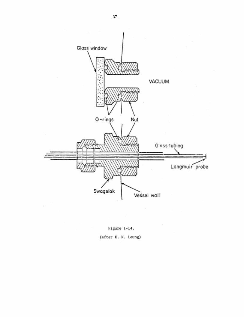
windows are installed on the side of the vessel, using swageloks as illustrated in Figure I-14. By simply

tightening the nut on the inner side of the vessel the 0-ring of the swagelok makes a good vacuum seal

against a flattened portion of the cylindrical wall. Using a 2" NRC oil diffusion pump and an Edwards

(ED-100) mechanical pump, an effective pumping speed of 285 liter/sec and a base pressure of 6 x 10-7

torr have been obtained.

The single vessel system with an external arrangement of magnets described above is easily

joined with another similar size vessel to form a double vessel system. In this case, the rim of the first

vessel is attached to the O-ring of flange A as seen in Figure I-16. The bottom of the second vessel is cut

away and then placed inside a deep O-ring groove of flange B. The two flanges are then clamped

together with another O-ring in between. Obviously a long multi-vessel system can be constructed by

applying this technique.

iii) Typical operating parameters for three representative D.C. discharge devices suitable for

introductory plasma experiments are summarized in Table I-4.

- 27 -

References

1. C. D. Child, Phys. Rev. 32, 492 (1911) I. Langmuir, Phys. Rev. 2, 450 (1913).

2. R. Limpaecher and K. R. MacKenzie, Rev. Sci. Instrum. 44, 726 (1973) UCLA PPG-114

(1972).

3. K. N. Leung, UCLA PPG-222 (1975).

4. S. Dushman, Scientific Foundations of Vacuum Techniques, 2nd Ed. (Wiley, New York)

1972.

5. G. Lewin, Fundamentals of Vacuum Science and Technology, (McGraw-Hill, New York)

1965.

- 28 -

- 29 -

- 30 -

- 31 -

- 32 -

- 33 -

TABLE I-4

OPERATING CONDITIONS FOR THREE TYPICAL REGIMES (Reference 3)

Device Characteristics: 24 liter volume, 30 cm diameter, 33 cm length, .92 mm wall thickness

5 tungsten wire filaments, .013 cm diameter (3 mil), 10 cm length

Discharge voltage = 60 V, Argon neutral gas

Surface MagneticConfinement

Plasma Density Neutral Pressure Total Discharge Current Filament HeatingCurrent(per filament)

None 2 x 108 cm-3 10-4 torr 1 amp 3 amp

Exterior surfacePermanent magnets

6 x 1010 cm-3 10-4 torr 1 amp 3 amp

Exterior surfacepermanent magnets

1 x 1012 cm-3 4 x 10-4 torr 10 amp 4 amp

- 34 -

- 35 -

- 37 -

- 38 -

- 39 -

- 40 -

Chapter II. Basic Plasma Diagnostics

One of the most important and frequently used plasma diagnostic techniques is the Langmuir

probe method. This method, which was first introduced by Langmuir1 about fifty years ago, can be

used to determine the values of the ion and electron densities, the electron temperature, and the

electron distribution function. This method involves the measurement of electron and ion currents

to a small metal electrode or probe as different voltages are applied to the probe. This yields a curve

called the probe characteristic of the plasma.

Another important technique, using microwaves, is frequently employed to measure plasma

parameters, especially in situations where it is difficult to insert probes into the medium. An

interferometer method is used to determine the phase shift of the microwaves transmitted through

the plasma and the average electron density is deduced from the amount of phase shift.

By combining the microwave or ratio frequency method with the probe technique, we can

measure the density to better than 1% accuracy. Electromagnetic waves propagating along a density

gradient with frequency o excite electron plasma waves at the critical density layer zo for which o =

p(zo), where p is the plasma frequency. Since the propagation of these electron plasma waves is a

sensitive function of the density profile, a careful mapping of the electron plasma wave propagation

characteristics will reveal the density along its propagation path. This more advanced method is

described in Chapter V.

1) Langmuir Probe

The fundamental plasma parameters can be determined by placing a small conducting probe

into the plasma and observing the current to the probe as a function of the difference between the

probe and plasma space potentials. The plasma space potential is just the potential difference of the

plasma volume with respect to the vessel wall (anode). It arises from an initial imbalance in electron

and ion loss rates and depends in part upon anode surface conditions, and filament emission current.

Referring to the probe characteristic, Figure II-l, we see that in region A when the probe

potential, Vp , is above the plasma space potential, Vs , the collected electron current reaches a

saturated level and ions are repelled, while in region B just the opposite occurs. By evaluating the

slope of the electron I-V characteristic in region B the electron temperature Te is obtained, and by

measuring the ion or electron saturation current and using the Te measurement, the density can be

computed.

The current collected by a probe is given by summing over all the contributions of the

various plasma species:I A n q vi i i

i

= ∑

(1)

where A is the total collecting surface area of the probe; vi = the average velocity of species I, and

vi =

1n

vf v dvi ( )r r

∫ for unnormalized f vi ( )r

. It is well known in statistical mechanics that collisions

among particles will result in an equilibrium velocity distribution f given by the Maxwellian function:

f v nKT

mExp

m v

KTαα

α

α

α

π( )

/r

r

=

−

−2

12

3 2 2

(2)

This distribution function is used to evaluate the average velocity of each species.

We will first consider a small plane disc probe which is often used in our experiments. When

it is placed in the xy plane, a particle will collide with the probe and give rise to a current only if it

has some vx component of velocity. Thus, the current to the probe does not depend on vy or vz.

The current to the probe from each species is a function of V º Vp - Vs.

I v nqA dvKT

mExp

m v

KTdv

KT

mExp

m v

KTy

y

z

z

( )/ /

=

−∞

∞

−∞

∞

∫ ∫2

12 2

12

1 2 2 1 2 2

π πα

α

α

α

α

α

α

α

⋅

∞

∫ dv vKT

mExp

m v

KTx x

x

v

212

1 2 2

π α

α

α

α

/

min

.

(3)

The lower limit of integration in the integral over vx is vmin since particles with vx component of

velocity less than vqV

mmin

/

=

21 2

α

are repelled, Figure II-2.

The integrals over vy and vz in (3) give unity so the current of each species is just

I v nqA dv vKT

mExp

m v

KTx xv

x

( )min

/

=

∞−

∫2

12

1 2 2

π α

α

α

α

(4)

- 42 -

a) The electron saturation current, Ies: In this region all electrons with vx component toward

probe are collected. We obtain the electron saturation current

I neA dv vKT

mExp

m v

KTneA

KT

mes x xe

e

e x

e

e

e

= −

−

= −

∞−

∫01 2

12

2 1 22

2π

π

/ /

(5)

Similarly, in region B and C where Vp < Vs and electrons are repelled, the total current is

I v I neA dv vKT

mExp

m v

KTis x xe

ev

e x

e

( )min

/

= −

−

∞−

∫2

1 212

2π.

(6)Substituting 1

22m v eVe min = − , (6) becomes

I v I neAKT

mExp

eV

KTise

e e

( )/

= −

2

1 2

π

(7)

since V < 0 in region B and C. Equation (7) shows that the electron current increases exponentially

until the probe voltage is the same as the plasma space potential (V = Vp - Vs = 0).

b) The ion saturation current, Iis: The ion saturation current is not simply given by an

expression similar to (5). In order to repel all the electrons and observer Iis, Vp must be

negative and have a magnitude near KTe/e as shown in Figure II-3. The sheath criterion2

requires that ions arriving at the periphery of the probe sheath be accelerated toward the

probe with an energy ~KTe, which is much larger than their thermal energy KTi. The ion

saturation current is then approximately given as

I neAKT

mise

i

=

21 2/

.

(8)

Even though this flux density is larger than the incident flux density at the periphery of the

collecting sheath, the total particle flux is still conserved because the area at the probe is smaller than

the outer collecting area at the sheath boundary.2-5

c) Floating potential V f : Next we consider the floating potential. When V = Vf, the ion and

electron currents are equal and the net probe current is zero. Combining equations (7) and (8), and

letting I = 0, we get

VKT

en

m

mfe i

e

= −

l

4

1 2

π

/

(9)

d) The electron temperature, Te : Measurement of the electron temperature can be obtained

from equation (7). For Iis < I we have

- 44 -

I v neAKT

mExp

eV

KTI Exp

ev

KTe

e ees

e

( )/

= −

=

2

1 2

π

(10)d n I

dV

e

KTe

l= .

(11)

By differentiating the logarithm of the electron current with respect to the probe voltage V for V <

0, the electron temperature is obtained. We note that the slope of lnI vs. V is a straight line only if

the distribution is a Maxwellian.

e) Measurement of the electron distribution function, fe(vx): The electron current to a plane

probe could be written in a more general expression as (again neglecting the ion current)

I nqA v f v dvnqA

mf qV d qVx x x

ev qV

= =∞ ∞

∫ ∫( ) ( ) ( )min

(12)dI

d qVf qV

( )( )α

where q = -e, the electron charge. This is a very simple way of obtaining the electron energy

distribution function. If we measure f(vx) as a function of plasma position, we can obtain the phase

space distribution f(vx,x). A further refinement is to observe the distribution at a given time t after a

certain event using a sampling oscilloscope. This results in the complete description, f(v,x,t), of the

electrons in a given system.

2) Double Probes5-8

A double probe consists of two electrodes of equal surface area, separated by a small distance

and immersed in the plasma, Figure II-4. One probe draws current I1 while the other is drawing

current I2. To find the electron temperature of the plasma, we consider quantitatively the current t o

the probe for various potential differences between the probes, Figure II-5. Since the probes are

floating at Vf of the plasma, i.e., the double probe circuit has no plasma ground (anode) connection,

the total current in the probe circuit must be zero. From (7) and (5), the current collected by probe

#1 is

I I is I es Expe V V V

KTf s

e1 1 1

1= −+ −

( )

(13)

Using the definition of the floating potential with (7),

I Expe V V

KTIes

f s

eis

( )−

=

- 46 -

(14)

hence (13) becomes

I I is ExpeV

KTe1 1

11= −

(15)

In the same manner we get

I I is ExpeV

KTe2 2

21= −

(16)

If the probe areas are equal, then (8) impliesI is I is Iis1 2= =

(17)

Zero net probe circuit current motivates the definition

I I I≡ = −1 2

Combining this with equations (15), (16), and (17) yieldsI I

I IExp

e

KTis

is e

−− −

=

ψ

(18)

where the double probe potential is defined by ψ ≡ −V V1 2 . Solving equation (18) for I

I Ie

KTise

= −

tanh

ψ2

(19)

Differentiating equation (19) with respect to ψ at ψ =0

dI

dI h

e

KT

e

KTise eψ

ψψ

ψ

= = − =

0

2

20

2sec

(20)

i.e., electron temperature is related to the slope of the double probe characteristic bydI

dI

e

KTiseψ

= −

2

(21)

The double probe can collect a maximum current equal to the ion saturation current and does

not disturb the plasma as much as the single probe with its anode connection. However, the small

amount of detected current (microampere range) does warrant a much more sensitive detection

circuit, as in Figure II-4.

The student is required to compare the electron temperatures and plasma densities obtained

with the single and the double probes.

- 48 -

3) Microwave Interferometer9,10

The basic idea behind this diagnostic scheme is as follows. The plasma acts like a dielectric

medium to electromagnetic radiation, and a wave propagating through the plasma will suffer a change

in phase

∆φ = −( )∫ k k dxvacuum plasma

L

0

(22)

where L is the path length of the plasma, kvacuum = w/c is the free space wave number of the

electromagnetic waves, and kplasma is the wave number of the wave propagating in the plasma, which

is given by the dispersion relation

kcplasma

pe=

−( )ω ω2 2 1 2/

(23)

Here w is the wave frequency, ωπ

pe

ne

m=

4 2 1 2/

, the electron plasma frequency and c is the speed of

light. If the plasma density is uniform over the distance L, we obtain from equation (23) for the

phase shift

∆φω ω

ω= − −

c

Lpe1 12

2

1 2/

.

(24)

a) Density measurement by phase shift: When wpe << w (note this restriction) we obtain a relation

between the phase shift and plasma density

∆φω ω

ω=

c

Lpe12

2

2 .

(25)

Defining the critical density by 4 2

2πω

n e

mc

e

≡ we can express equation (25) alternatively by

n

n k Lwhere k

w

cc vacvac= ≡

2∆φ,

(26)

Since all laboratory plasmas have a certain degree of inhomogeneity, i.e., some density

gradient, the phase shift Df is an integrated quantity as represented by equation (23). However, the

density profile can be obtained by relative density measurement using movable probes. If we write

n(x)=n0f(x), where f(x) contains the spatial variation in the plasma density, a relation similar t o

equation (26) can be achieved using

- 50 -

nn

k f x dx

c

vac

L0

0

2=

∫∆φ

( )

(27)

Thus with the help of the radial probe measurement on the relative density profile, the microwave

interferometer technique could be used to obtain the absolute density at any radial position.

b) Observation of cut-off: For w = wpe the relation given by equation (26) or (27) is no

longer valid (why?). One must use equation (23) or (24) directly and the relation between Dy and n

becomes quite complicated. However, when w = wpe, the wave number becomes purely imaginary and

no propagation is possible. By observing the cut-off, we can calculate the maximum density in the

plasma, nmax = nc, where nc is the critical density defined above. The student is required to compare

this microwave method with the Langmuir probe result.

4) Experimental Procedure

a) Follow the procedure as described in Chapter I to obtain a D.C. discharge. Clean up probes

and set up a sweeper circuit as described in Appendix A. Observe a Langmuir characteristic curve by

using the oscilloscope. For recording, the single sweep mode must be used with sweep rate of 1 to 2

seconds per cm, such that the mechanical movement of the recorder pin can follow the changes of

the signal. The manual sweeping circuit of Figure II-7a is a possible substitute for oscilloscope and

automatic sweeper when recording the Langmuir curve graphically.

b) Details of the probe characteristic: Take several single probe traces using the probe

sweeper circuit and the x-y recorder. Replot each trace on semi-log paper and subtract out the ion

saturation current to obtain the current contributed by the secondary electrons. At low neutral

pressures the primary electron current will appear as a long, high temperature (gently sloping) tail

with negative current in the ion saturation region of probe bias. In this case, subtract the primary

electron current (as well as the ion saturation current) from the total probe current to obtain actual

secondary electron current. (Primary electron current collected for a given probe bias can be

estimated by extrapolating the straight-line primary tail.) Obtain the electron temperature from the

slope of the curve and the density from both the ion and electron saturation currents.

Experimentally determine how the ratio Ies/Iis depends on the mass ratio.

You will find that the primary electron current usually overshadows the ion current.

However, the ratio of primary electron to ion current can be reduced significantly and the ion

saturation current can be observed by simply raising the neutral pressure to about 10-3 torr (explain

why).

c) Double probe: Set up the double probe manual sweeper circuit with the x-y recorder and

obtain a double probe trace. Compute the density and electron temperature and compare the result

- 52 -

with n and Te obtained from a single probe characteristic at the same time in the same region of the

plasma.

d) Microwave interferometer: The X-band microwave interferometer set-up is shown in

Figure II-6. Microwave signal generated by the oscillator is split into two paths, one propagating

through the plasma, V1 cos (wt + o1), the other through a variable phase shifter to provide a

reference signal, V2 cos(wt + o2). The signal propagating through the plasma is received by a pickup

horn on the other side of the vacuum system, and then added to the reference signal by the magic

tee: Vsum = V1 cos (wt + 01) + V2 cos (wt + 02). This signal is then fed into a crystal detector, which

produces a current signal I V2sum. By taking a time average of the current I from the crystal,

I V V V VVsum∝ = + + −2 12 1

2 12 2

21 2 1 2cos( )φ φ

(28)

For a given plasma density, f1 is fixed. Vary V2 with the variable attenuator and f2 with the phase

shifter to obtain a null (f1 f2 = p). Be careful not to overattenuate the reference signal V2 as this

will result in a phase independent signal [V2 = 0 in (28)].

The crystal diode output signal is so small that a high gain amplifier must be used.

Furthermore, the microwave signal should be gated on and off (i.e., square wave modulated output) t o

avoid confusion over D.C. shifting of the output signal in the high gain amplifier.

Turn off the plasma (by turning off the discharge), find the null again and record Df. In

finding the null, large errors can develop. To minimize these, plot <Vsum2> versus fz for the case

where the plasma is present and the case where it is turned off to obtain two cosine curves offset by

phase Df. Although this procedure is tedious, it is recommended for improved accuracy.

Calculate the plasma density using equation (26) and compare the results with those obtained

from the probe measurements. If the density is non-uniform, try to correct the result by measuring

relative density profile using a movable Langmuir probe. Difficulties arise whenever the dimensions

of the plasma container are comparable to the wavelength of the microwaves. In this case, the

waveguide horn is not large enough to sharply define the microwave beam and unwanted cavity

modes are excited in the vacuum chamber as a result. These modes have multiple paths through the

plasma and can drastically alter the measurement of Df. Hence, steel wool has been placed near both

the sending and receiving horns to attenuate these undesirable multiple path signals.

e) Density Measurement via Plasma Resonance: The most accurate local density

measurement in an inhomogeneous plasma is achieved by exciting the local plasma resonance p(x).

An oscillating electric field of frequency w0 is externally excited in the plasma by a capacitor plate

oriented to give an electric field along the density gradient as shown in Figure II-7. Where ever the

- 54 -

external frequency matches the local plasma frequency 0 = p(x0), the amplitude of the external

electric field is found to be enhanced by an order of magnitude or more. This resonance is best

detected by noting the deflection of an electron beam traversing the resonant location (Figure II-7)

in a direction perpendicular to the density gradient. (A detailed description of this electron beam

diagnostic is to be presented in Chapter V.) Since the external oscillating field frequency 0 can be

precisely measured, the plasma density can be determined to better than 1%. A Langmuir probe can

be calibrated using this technique.

Questions

1. Why does the ion saturation current depend on kTe?

2 If there is an excess of primary electrons in the plasma, what kind of effect can one see by using

(1) single probe, (2) double probe, and (3) microwave interferometer? Can you measure the

density of the primary electrons?

3. For a plasma consisting of positive and negative ions of equal mass, draw the probe

characteristics, carefully labeling the quantities Is+, Is-, Vf and Vs. How do you deduce T+ and T-?

4. What processes determine potential difference between the plasma and the anode?

5. When a fine conducting grid (called "plasma demon") is biased to some positive potential, it was

found that the electron temperature increases by a factor up to 2-3. Can you explain this effect?

5) Appendix A: Description of Probe and Circuitry

a) Langmuir probe: A typical disc Langmuir probe in our laboratory experiment is spot welded

onto a 0.010" diameter tungsten wire extending from the end of a glass insulating tube which is

surrounded by a ceramic support sleeve, [c.f. Chapter I, Figure I-14]. A circuit diagram which is

useful for plotting the current-voltage characteristics on an x-y recorder is given in Figure II- 4.

The probe voltage is obtained from a stabilized power supply (0 to 100 V), or better still a large

battery, and can be varied in polarity and magnitude with a potentiometer. The probe voltage is also

monitored on the x-axis of an x-y recorder which is easily calibrated with a voltmeter. As in Chapter

I, the probe current is found from the voltage drop across a small resistor. The y axis is most

conveniently calibrated by replacing the probe with a known resistor. More sophisticated circuits

which electronically generate a voltage ramp may also be used to obtain probe I-V characteristics.

One of these is shown in Figure II-8b.

The Langmuir characteristic is obtained by sweeping the probe voltage slowly between the

negative and positive limits so as to include all the important regions of the curve.

c) Double probe: The double probe used in these experiments consists of two planar discs

separated by a small distance. An alternative circuit to that of Figure II-4, suitable for

measuring the double probe characteristic is the same as shown in Figure II-7, except that

the ground (anode) is replaced by the second probe. No part of this circuit should be

grounded. Each component probe of the double probe should be cleaned in the same manner

as the Langmuir probe.

- 56 -

References

General Langmuir Probe

1. 0. Mawardi, Amer. J. Phys. 34, 112 (1966).

2. F. F. Chen, "Electric Probes," Plasma Diagnostic Techniques, Ed. by Huddlestone and Leonard

(Academic Press, 1965).

3. F. F. Chen, C. Etievant and D. Mosher, Phys. Fluids 2, 811 (1968).

4. J. G. Laframboise, "Theory of Spherical and Cylindrical Langmuir Probes in a Collisionless,

Maxwellian Plasma at Rest," UTIAS Report #100, Univ. Toronto (1966).

5. L. Schott, "Chapter 11," Plasma Diagnostics, Ed. by W. Lochte -Holtgreven (North Holland,

1968).

Double Probe

6. F. Johnson and L. Malter, Phys. Rev. 80, 59 (1950).

7. S. Ariga, J. Phys. Soc. Japan 31, 4, 1221 (1971).

8. P. Demchenko, L. Krupnik and N. Shulika, Sov. Phys. -Tec. Phys. 18, 8, 1054 (1974).

Microwave in Plasmas

9. C. Wharton, "Microwave Techniques," Plasma Diagnostic Techniques.

10. M. Heald and C. Wharton, Plasma Diagnostics with Microwaves (Wiley, 1965).

- 58 -

Chapter III Energy Analyzer

While a simple plane probe yields information on the electron density and temperature, an

ion energy analyzer using additional electrodes to eliminate the electron contribution is required t o

measure the ion temperature. In this chapter we will discuss its design, practical applications as well as

its limitations.

1) Energy Analyzer Design

One design of an ion energy analyzer as depicted in Figure III-l has been found to possess

adequate resolution for the study of ion distribution functions. It consists of two mesh grids (Gl and

G2) and a collector plate (P) located behind the grids.

The first grid is left at the plasma floating potential so that it repels electrons but allows

most ions to pass through. The second grid1, called the discriminator, is biased positively in order t o

retard those ions with energy per unit charge less than its potential φ, measured with respect to the

plasma potential. The collector plate, which is biased very negatively (typically ~60 V), repels the

residual high energy electrons which penetrate through the first grid and collects all the ion current.

A schematic of the relative potentials of different electrodes is shown in Figure III-2. The

placement of the analyzer and the physical connections to its various electrodes are depicted in

Figure III-3. The sawtooth output of a scope is used to provide a ramp for a electronic sweeper

which drives the discriminator. A display of the collector current vs the sweep voltage is shown in

Figure III-4.

1 Do not overbias the discriminator grid. The large electron current it collects can burn

out the fine mesh.

- 59 -

- 60 -

- 61 -

- 62 -

- 63 -

Ideally, the electric field inside the analyzer should point axially along the direction in which

the velocity component is to be analyzed. To achieve this, the hole size h of the mesh forming the

grid and the spacing s between adjacent electrodes must be of the order of 1 - 10λD. Each grid then

forms an equipotential surface with the discriminating electric field oriented perpendicular to the gird

surface. At higher plasma densities or larger mesh sizes such that h, s > > λD, the plasma in between

grid wires shields out the potential of each wire, giving rise to short-range radial electric fields

between plasma and grid wires. Particles going through the grids no longer see an axial discriminating

electric field and poor resolution of the ion distribution results. The finest mesh presently available

satisfies the above size criterion up to a plasma density of 1012/cm3. If the first grid is made of such a

fine mesh it lowers the plasma density inside the analyzer by as much as two orders of magnitude and

increases λD there by an order of magnitude. As a result, the allowable mesh size of the second grid is

somewhat larger. The lowering of plasma density inside the analyzer is a desirable feature, as long as

the collector current is within the limit of detectability, since the plasma behaves more like a

collection of single particles whose trajectories are easily predicted. If the ion energy exceeds 10 eV

sputtering and secondary emission from the electrodes must be taken into account. A fourth grid

might have to be introduced in front of the collector and biased slightly more negatively than the

collector in order to repel secondary electrons released from the collector surface due to ion

bombardment. If allowed to escape from the analyzer probe, this secondary electron emission will

result in a stray, positive collector current.

2) Analysis of Measurements

After the electrons have been screened out by the discriminator grid, the ion current reaching

the plate collector of area A is given by

I eA v F v dve

M

( ) ( )/φ φ=

∞

∫ 2 1 2

(1)

=

= =

∞ ∞

∫ ∫eA

MF v d

Mv eA

MF v dE where E Mve

Me

( ) ( )/22

1 2

212

φ φ

Differentiating (1) with respect to φ, we get an expression for the velocity distribution function F(v)

or G(φ) in terms of the first derivative of the current-voltage characteristic, I(φ) vs φ, namely

F vM

e A

dI

d( ) = − 2 φ

(2)

- 64 -

Let us consider a typical characteristic of I(φ) vs φ as in Figure III-4a. The derivative dI

dφ obtained by

methods mentioned below is represented in Figure 4b. This gives us the ion distribution as a function

of energy. If the velocity distribution function F(v) vs v is desired the abscissa must be re-scaled

according to the relation ve

M= 2 φ , as in Figure 4c. It should be pointed out that the I(φ)

characteristic should not be taken seriously at very low discriminating voltage φ, when the electric

fields introduced by the analyzer grids are comparable to the fluctuating fields inside the analyzer. In

practice the shape of the distribution is taken to be the curve starting from the right side in Figure 4b

and rising to a maximum near φ = 0 V. The left side of the maximum is discarded on account of the

poor resolution of the analyzer.

Ion Temperature

If F(v) is a Maxwellian function then, according to (1). I(φ) =

)KT

e(-(constant)=)I(

i

φφ Exp or

KT

e-(constant)=)I(

i

φφln

The plot of

ln I(φ) vs. φ

should be a straight line ant the inverse of its slope gives the ion temperature KTi directly.

Plasma Potential

The analyzer also measures the plasma potential, i.e. the potential at which all ions are

collected. Experimentally this potential is given by the value at which φφ

d)dI(

reaches a maximum.

- 65 -

- 66 -

3) Experimental Methods of Differentiation of Current-Voltage Characteristics

Ion distribution functions can be obtained from electronic circuits which differentiate the

normal current-voltage characteristic of the analyzer with respect to φ, Figure III-4b.

Experimentally, this differentiation can be carried out in two different ways: with a simple R-C

differentiating circuit, Figure III-5a, or a more sophisticated method using a lock-in detector, Figure

III-5b.

i) R-C differentiation

This method requires a very linear variation of the discriminator voltage φ with time t. With

the R-C differentiator synchronized with the discriminator voltage ramp, differentiation is carried

out with respect to time and therefore indirectly with respect to φ. The advantage of this method is

ifs fast response and instant display of the distribution function.

An oscilloscope plug-in unit which has an operational amplifier differentiation circuit is used.

When the analyzer's collector signal Vi is put into the circuit, shown in Figure III-5a, the output is

simply

V RCdv

dti

o ≅ −

ii) Differentiation by synchronous detection

In this method a small sinusoidal voltage φ1 cos ω0t is applied to the discriminator grid biased at

potential φ0 and the synchronous variation of the current as a function of energy selection potential

is measured. The current collected is

IeA

MG E dE

e( ) ( )φ

φ=

∞

∫(5)

Adding a small amplitude modulation φ1 cos ω0t to the linear variation of discriminator bias φ0

we define

φ ≡ φ0 + φ1 cos ω0t, with φ1 << φ0.

- 67 -

Then expanding (5) in a Taylor Series about φ0 produces

+|d

Id2

)t(+|

d

dIt)w(+)I()I(

00 2

2201

010 φφ φωφ

φφφφ

coscos_ …

(6)

By looking at the coefficient of the time varying component φ1 cosω0t we can find |ddI

0φφ and hence

the distribution function G(eφ0) according to (5).

Figure III-5b shows a schematic diagram for the measurement of ion distribution functions with

the aid of a lock-in detector.

A lock-in detector is a ultra-sensitive instrument, capable of detecting a small signal (signal-to-

noise ration as low as 40 db), provided this signal varies at the same frequency as a known reference

signal. It is generally used to multiply some input signal ΣnAn cos ωnt by a reference signal Brcos ωrt

and then time-average the product: the lock-in output signal S is then

>)]+t(Bt)[A(=<S rrnnn θωω coscosΣ

(7)

>)+t( t)(BA=< rrrr θωω coscos

= lim cos cos1 2

0TA B w t dt

Tr r r

Tθ∫

→ ∞

- lim cos sin sin1

0TA B w t w t dt

Tr r r r

Tθ∫

→ ∞

This final term time averages to zero, hence

. 2BA = S rr θcos (8)

- 68 -

The final result is proportional to the signal strength at the frequency ωr and is related to the angle θ

between the reference and its corresponding harmonic in the input signal. All other frequency

components do not maintain a constant phase relationship with the reference signal and are time

averaged to zero.

To relate this lock-in output S to the measurement of |ddI

0φφ in (6), write the reference

component in (7) as Br cos ωrt = φ1 cos ω0t and the input signal as ΣnAn cos ωnt = I(φ). According t o

(8) the detector output

)(e |d

dI

2 = S

0

21

0φ

φφ

φ ∝

is proportional to the ion energy distribution function.

4) Experiments with the Ion Energy Analyzer

Perform each of the following experiments in the double plasma (DP) device described in

Chapter 1, Appendix B.

a) Ion temperature measurement: Monitor the probe characteristics on both sides of

the DP device and

vary the known bias between the two chambers to balance the plasma potentials1 so that ion beams

are not present in either chamber. Obtain an analyzer I-V characteristic for at least two different

neutral pressures. Replot the characteristic on semi-log paper and determine the ion temperature.

Determine the plasma potential according to the potential φ at which φddI

reaches a maximum

[Figure III-4(b)]. Compare this measurement with the one made by the Langmuir probe.

b) Observation of ion beams: Bias the source chamber positive with respect to the target

chamber to launch an ion beam. The beam energy is determined by the difference in plasma

potentials between the source and target plasmas. Record an I-V characteristic to determine Ti and

Tb, the temperature of the beam, from the slope of a semi-log plot of this data.2 An example is

given in Figure III-6, 7 in which the I-V characteristics ant the corresponding ion distributions are

depicted. When a beam is directed into the analyzer, all the beam ions are collected whenever the

discriminator potential φ is such that eφ< Eb, where Eb is the beam energy. For

eφ > Eb, the beam ions are repelled so the I-V characteristic has the step function shape as in Figure

1Because of slight density gradients near the DP interface, plasma potentials are most

easily balanced when each Langmuir probe is placed about 10 cm from the launching grid.

2See Appendix A

- 69 -

III-6b and III-6c. When the I-V characteristic is differentiated to obtain the ion velocity distribution

function, F(v) vs. E, the ion beam appears as a bump on the tail centered around the beam's energy as

in Figure III-7b and III-7c.

Obtain similar ion velocity distribution functions for beam energies such as 2 eV, 4 eV, 10 eV,

using the operational amplifier plug-in for R-C differentiation. Verify the beam energy obtained

from the analyzer against the potential difference between target and source chambers.

In preparation for the next chapter, monitor the density fluctuation (δn/n) in the target

chamber with a Langmuir probe and see if there is a correlation between the fluctuations and the

beam energy. What beam energy and corresponding ion beam velocity maximizes the amplitude of

the fluctuations?

c) Ion beam decay-measurement of the charge exchange cross-section: The ion beam decays

spatially due to charge exchange collisions1 and elastic collisions with the background neutral atoms.

To derive an expression for this spatial decay, we note that a decrease dIb in the beam current in a

distance dx at the point where the beam current is Ib is proportional to -NoIbdx, where No is the

neutral density. The proportionality constant is the charge exchange cross-section, σ, which may be

visualized as the effective area a neutral atom presents to an incident beam ion for undergoing a

charge exchange collision.

1When a beam ion A+ collides with a cold neutral A, the ion A+ may capture an electron

from the atom A in accordance with

A+ + A → A + A+

(fast ion) + (slow neutral) → (fast neutral) + (slow ion)

resulting in a fast (beam) neutral and a cold ion. This charge-exchange process is utilized incurrent plasma fusion studies where intense neutral beams are produced from fast ion beams forthe purpose of injection heating.

- 70 -

- 71 -

Thus

dIb = -IbN0σdx

Integrating we have

ln Ib = ln I0 - N0σx

or

Ib = I0 Exp (-N0σx).

(9)

The beam current therefore decays exponentially. The cross-section can be computed by simply

measuring the e-folding decay length of the beam with the energy analyzer and assuming the cool

neutrals to be at room temperature.

Experiment

Vary the axial position of the analyzer for one beam energy and plot the spatial decay of the

beam for at least two different neutral pressures (10-4 and 8 × 10-4 torr for example). Use (9) above

to measure the collision cross-section for the beam energy you choose and compare it with the cross-

section for both elastic and charge exchange collisions in Reference 8 or 9. According to your data,

which collision process dominates?

- 72 -

References

1. J. Brophy, Basic Electronics for Scientists, 2nd Ed. (McGraw-Hill, 1972) p. 318.

2. S. Brown, Basic Data of Plasma Physics (MIT Press, 1967).

3. E. McDaniel, Collision Phenomena in Ionized Gasses (Wiley, 1964).

- 73 -

5) Appendix A: Ion Beam Temperature in Double Plasma Device

The ion beam-plasma system is formed in the DP device by biasing the source chamber anode

positive with respect to the target chamber anode. This results in a source plasma space potential

which is higher than the potential of the target plasma. If the difference between the source and

target space potentials is ?, then we have the situation shown in Figure III-B, where the space

potential is1

0 x ≤ 0

φ(x) = φ(x) 0 < x < L

-φ x ≥ L

Because the dynamics of the accelerated beam ions is of interest, a kinetic treatment (rather than

fluid theory) is appropriate. We start with the collisionless, steady state 0) = (tf

∂∂

Boltzmann

equation given by

0 = v

f

m

qE +

x

fv

xx ∂

∂∂∂

for each component plasma species, where x- = E ∂

∂φ. This equation is satisfied by the distribution

function

)KT

(x)q -

2KTmv(- C = v)f(x,

2 φExp ,

with C ≡ constant, as can be verified by direct substitution.

In the source chamber, the plasma ion distribution function is just a Maxwellian (Figure III-9a):

)KT2

Mv(- C = (v)fi

2

i Exp

From Figure III-8 it is obvious that only those source plasma ions (near the plasma-grid sheath

interface at x = 0) with v x > 0 can enter the grid sheath to become accelerated beam ions hence,

the restricted velocity distribution of Figure III-9b.

As these extracted plasma ions proceed as beam ions down the potential "hill" plotted in Figure

III8, they will all gain the same amount of energy Eb, where Eb ≡ eφ. Because of this, the beam ions

arriving at the end of the sheath (x = L) will have a minimum velocity vo given by

vEMo

b≡ 2

1Source plasma potential is chosen as ground reference to simplify the mathematical

analysis which follows.

- 74 -

- 75 -

Also,

N C Expv v

advb v

i

= −

∞

∫0

02 2

2

=

∞

∫C Expv

aExp

v

adv

i iv

02

2

2

20

=

C a Expv

aerfc

v

aii i

02

20

2π

where

erfc z Exp u duz

( ) ( )≡ −∞

∫2 2

π

with z denoting the minimum beam ion velocity normalized to plasma ion thermal velocity zv

ai

≡ 0 ..

>)v - m(v< = KT 2

1 2

1

2

Nm v v f v dv

v

v( ) ( )−∫ ,

(10)

where v1 and v2 are the lower and upper velocity limits, respectively; the normalization factor, N, is

given by

N f v dvv

v≡ ∫ ( )

1

2

and the average velocity, v , is

vN

vf v dvv

v= ∫1

1

2

( )

In the source chamber, plasma ions have v1 = -∞, v2 = +∞ and

f vM

KTExp

Mv

KTii i

( ) =

2 2

1

2 2

π.

Equation (10) yields an identity for this case.

However, for the accelerated beam ions at x ≥ L, we have (referring to figure III-9c) v1 = v0, v2

= +∞, and

f v C ExpMv

KT

E

KTbi

b

i

( ) = +

2

2,

where C is a constant.

- 76 -

(11)

- 77 -

We also need to find the average beam ion velocity vb before KTb can be computed from (11):

vbC

Nv Exp

v v

adv

b iv

= −

∫ 0

2 2

20

= − =∫C

NExp z a Exp y dy y

v

abz i

i

( ) ( ) ,2 22

2

122

)z(- )z( N2

Ca= 22

b

2i ExpExp

(z) erfc

)z(- a =

2

iπ

Exp

With the definition

ξπ

( )( )

( )z

Exp z

erfc z≡ − 2

we proceed to evaluate v:

< >= −

∞

∫vC

Nv Exp

v v

adv

b iv

2 2 02 2

20

=−

∞

∫ v Expv

adv

a erfc z

iv

i

22

20

2π

( ).

Changing the variable in the last integral to w≡av

i and integrating by parts gives

)a

v(av + a2

1 = >v<

i

0i0

2i

2 ξ

Using these expressions we can evaluate >)v - (v< 2b in (11) above by noting that

>v + v2v - v< = >)v - (v< 2bb

22b

v + >v<v2 - >v< = 2bb

2

v - >v< = 2b

2.

Thus according to (10):

]])a

v(a[ - )a

v(av + a2

1 M[= KT

2

i

0i

i

0i0

2ib ξξ

- 78 -

(z)].2 - (z)2z + [1 z2

Mv = 2

2

20 ξξ (12)

The low ion temperature Ti typical of DC discharges implies that

ai << v0 or z >> 1.

The following asymptotic expression can be used:

πz Exp z erfc zi

z ii

( ) ( ) ~( )

( )2

21

11 3 5 2 1

2+ ⋅ ⋅ ⋅ ⋅ ⋅ ⋅ −

=

∞

∑Keeping only the terms of order 1/z4 or larger in the denominator we get:

3 + z2 - z4z4

=

z4

3 +

z2

1 - 1

z (z)

24

5

42

_ξ

Placing this expression for ξ(z) into (12) gives

])3 + z2 - z(4

9 + z12 - z28 + z8[ KT = KT 224

246

ib

(13)

(Since z is large, the term inside the brackets is clearly positive, as it should be.) Note also as z → ∞

we get

KTKT

z

KT

VA

KT

ebi i

i

i~2 2 2

020

2

2

0

=

= ( ) → +φ.

Hence the temperature of the beam is less than the source temperature KTi andapproaches zero as V

ai

0 → ∞.

- 79 -

Chapter IV. Ion Acoustic Waves

In this and in the following chapters, we are going to examine the excitation and propagation

of plasma wave modes. ln a plasma with no applied magnetic field, the wave phenomena are

particularly simple because such a plasma has only two electrostatic normal modes--a high and a low

frequency mode. The high frequency mode is one in which the electrons oscillate rapidly about

stationary ions and is called the electron plasma wave. In the low frequency mode, ions and

electrons oscillate in phase producing longitudinal density perturbations called ion acoustic waves.

They were first predicted in 1929 on the basis of a fluid analysis by Tonks and Langmuiral1 who

found, for frequencies well below the ion plasma frequency and for isothermal changes, that the

phase velocity vp should be given by

).M

KT + KT( vie2

p ≅

These waves differ from ordinary sound waves in that the coupling between electrons and ions arises

from electric fields resulting from small charge separations. More recently, a number of authors2,3

have shown on the basis of the collisionless Boltzmann (Vlasov) equation that ion waves can exist

in a plasma even in the absence of collisions. The collisionless equations also predict an interesting

feature of the ion waves namely, that they should be damped by interaction with ions moving with

velocities close to the phase velocity of the wave.4 This damping, which was first predicted by

Landaus for electron plasma waves, is strong in the ease of ion acoustic waves even for wavelengths

large compared with the Debye length, if the ion and electron temperatures are comparable.

Ion acoustic waves can be excited by producing a density perturbation with a conducting

launch grid immersed in the plasma. Two commonly used techniques are described as follows:

i) Absorption method:6 Consider a grid immersed in the plasma as shown in Figure IV-la.

If the ion-collection region (approximately 10 λd) is a significant fraction of the interwire spacing,

then a modulation of the grid bias will produce a varying amount of absorption, i.e., a small density

perturbation is created in the transmitter probe vicinity and propagates down the plasma column.

ii) Velocity acceleration: A second method uses velocity accelerations produced by biasing

the potential of one plasma with respect to another as shown in Figure IV-lb. The inflow of plasma

- 80 -

- 81 -particles from one chamber to another sets up a density perturbation. In this case, a floating wire-

mesh grid defines the interface of the two plasmas.

Most excitation schemes create a propagating density perturbation by a combination of these

two methods. However, there are more advanced methods which do not require grids in the main

region where ion waves are excited and detected. For example, a slow electron drift can cause ion

waves to grow spatially from one end of a device to the central region by an order of magnitude a

large amplitude electron plasma wave excited by electron beams or externally imposed

electromagnetic waves can decay into an ion acoustic wave ant another electron plasma wave of

slightly lower frequency. These advanced methods will be treated in Volumes II ant III.

1) Physical Description

Ion acoustic waves derive their name from the similarity they bear to sound waves in a gas.

Sound waves are longitudinal density oscillations in which the compressions and rarefactions are

driven by collisions among the gas atoms. Ion acoustic waves are also longitudinal density

oscillations, but they are driven by collisionless effects--namely, the electric fields that arise from

the space charge developed by the slight displacements between ion and electron density

perturbations. Since the ions and electrons oscillate in phase, the ion space charge, which would

normally tend to push the ion compressions apart, is neutralized or shielded by the electrons.

However, due to their thermal motion, some electrons overshoot the ion charge clouds hence the

shielding is incomplete and an electric field is developed which then drives the wave. The higher the

electron temperature, the more incomplete the charge neutralization and the greater the wave electric

field and the phase velocity.

If the electron-to-ion temperature ratio is such that Te/Ti >> 1, a condition that can be met

in laboratory plasma, the dominant driving force comes from the electron pressure, and the ion

acoustic speed is simply given by Cs = [γeKTe/M]1/2. The ratio of specific heats, γe and γi, can be

assigned values from simple thermodynamic arguments. Since the frequency of the ion waves is so

low, the electrons move several wavelengths in one period and thus carry away any heat developed

- 82 -within that period. Therefore, the isothermal condition is valid for electrons, and γe = 1. The ion

compressions, however, are one-dimensional, γi is generally assumed to be 3. A comparison of fluid

theory and the more exact kinetic theory (Appendix A) of ion acoustic waves shows that the above

values of γe and γi give an excellent approximation to the exact result.

2) Simple Theoretical Derivation

a) Linear dispersion of ion acoustic waves: We will first present a very simple fluid model,

which reveals the wave motion carried by the bulk of the two charged species: ions and electrons.

Various refinements are then added to explain experimental observations. A more complete kinetic

theory, which includes interactions between waves and resonant particles as well as boundary

conditions at the exciter, is treated in Appendix A.

i) Elementary analysis: We shall first present a simple analysis of ion acoustic waves under

the following assumptions:

1) Ti = 0, which to a good approximation describes our plasma with Ti << Te .

2) Assume charge neutrality ni = ne = n. This is a good assumption for low frequency waves

in which ions and electrons move very nearly together.

3) Ions provide the main inertia since Mi >> me. Neglect electron inertia.

4) One-dimensional analysis since our plasma has a large cross section and the excited wave

is very nearly a plane wave.

Ions and electrons are described as charged fluids according to the following equations:

neE = dtdvnM i

(1)

nmdvdt

= - neE - p

xe e∂

∂(2)

Adding equations (1) and (2), and using assumptions (2) and (3), we obtain:

nM dvdt

= -p

x = - KT

nx

,i ee e

∂∂

∂∂

γ

where the adiabatic assumption pe ∝ nγe is used:

γe = ratio of specific heats for electrons = (r+2)/r,

- 83 -where r is the number of degrees of freedom.

Using the continuity equation for ions, assuming small wave amplitudes and linearizing (making

use of n1/n0 << 1, where n1 is the time dependent density term, and neglecting second order terms),

we obtain the wave equation:2

2e e

2

2

n

t = KT

Mn

x.∂

∂∂∂

γ

Assuming one-dimensional plane waves of the form Exp i(kx - ωt) yields the following dispersion

relation:

ω2 = k2Cs2,

where the phase velocity

2s

e eC = KTM

.γ

ii) Refinements:

1) Including the ion temperature and hence the ion pressure in equation (1) we obtain:

2

2

2s

eKT i i

k = C =

+ KTM

eω γ γ(3)

2) Next we include the wave electric field from the Poisson's equation

∂∂Ex

= 4 e(n n ).i eπ (4)

Under the assumption of small electron inertia, equation (2) yields a relationship between ne and the

local plasma potential φ:

e 0e

n = n [e

KT].Exp

π(5)

Inserting the relation (5) into equation (4) we obtain2

2 1 oex

= 4 e(n n [e

KT]).∂

∂π π φ

Exp

Writing ni = n0 + n1 , and noting that plasma density (n0 kDe-3 >>1) justifies the assumption eφ/KTe <<

1, we have for the wave potential

φ π =

4 en

k + k,i

2De

2 (6)

Now we include the finite ion temperature in equation (1) and rewrite it as

- 84 -

nMt( ) = n e

E KT

nio i i

2i

2

∂∂

∂∂

∂∂

∂∂

ν γx x x

= n e KTn

o

2

2 i i

2i

∂∂

− ∂∂

φ γx x2

(7)

Again using the continuity equation,2

i2

o2

2i i

2i

2

n

t =

n eM

+ KTM

n.∂

∂∂∂

∂∂

φ γx x

Fourier transforming and using (6)2

2

e

De

i is

k = KT

M

1

1 + (k k )

KTM

C ,ω γ∑ 2

2

2

+ ≈ (8)

which lacks the factor γe of equation (3) because of the assumption of equation (5), i.e., γe = 1.

This dispersion relation is plotted below in Figure IV-2. At low frequencies and small

wavenumbers, the dispersion curve is linear and has intercept at ω = 0 so that in this region the phase

and group velocities are identical. Since we have not considered any dissipation process in our

theoretical treatment so far, the wavenumber k is real. At higher frequencies and wavenumbers, the

curve bends over and the wave becomes dispersive that is, the phase velocity becomes a function of k

(it decreases with increasing k).

b) Wave damping:

i) Collisional damping by neutrals: ln a weakly ionized laboratory plasma where the neutral

density is much higher than the plasma density, the dominant damping mechanism of ion acoustic

waves is ion-neutral collisions. We may derive an expression for the spatial damping rate by including

a collision term in the equation of motion for the ions,

Mn ( vt

+ v + Mn = enE p

,ii

ii

i in i ii∂

∂∂∂

− ∂∂

ν ν νx x

(9)

where νin is the ion-neutral collision frequency.

Using equation (9) to replace equation (7) in our previous derivation and solving for the

dispersion relation, we obtain for the weak damping case

k C

iC

s

in

s

≈ +−

+

ω ν .

2(10)

Equation (10) shows that for weak damping the wavenumber has a real and an imaginary part. Since

the wave varies in space as Exp ikx, the imaginary part of the wavenumber will produce spatial

exponential damping proportional to Exp[-υinx/2Cs]. The distance the wave travels before its amplitude

- 85 -is reduced to e-1 of its initial value is then

- 86 -

δ ν C ,s in≡ 2

and the number of wavelengths in this distance is

δλ π

ωπν

1/ k2 /k

= ,i

r in

≡

- 87 -

where

k = kr + iki

If νin << ω, δ/λ >> 1 and we expect to see many wavelengths over the e-folding distance. In particular,

if the frequency is raised, the collisional damping will effectively decrease.

ii) Ion Landau damping: The total damping of ion acoustic waves will not continue to decrease

as ω approaches ωpi because the phase velocity becomes comparable to the ion thermal velocity and

there are resonant wave-particle interactions. Ions moving slightly slower than the wave can be

accelerated and transfer energy out of the wave, thus damping it collisionlessly. Similarly, ions moving

slightly faster than the wave can transfer their energy to the wave and make its amplitude grow. In a

Maxwellian plasma there are more ions moving slightly slower than the wave and the net effect is

damping. This collisionless damping due to the resonant wave-particle interaction is called Landau

damping and is named after the discoverer of a similar effect for electron plasma waves. Kinetic

theory (Appendix A) shows that the rate of Landau damping is proportional to the slope of the ion

distribution function ∂ ν ∂ν νfop

( ) evaluated at the phase velocity:

ki = (attenuation distance)-1 ∝ ∂∂

f( )

| pvνν

∝ − ∝ − −

[a

] 1

2TT

,pp e

i pii

νν ω

ωExp Exp

2

2

2

21

where equation (8) has been used for the expression of the phase velocity vp. The above expression

holds only in regimes where the damping is weak, ki/kr << 1; for example Te/Ti >> 1, vp >> ai.

As the excitation frequency ω approaches the ion plasma frequency ωpi, the phase velocity vp

is reduced (Figures IV-2 and IV-3) and moves closer to the region of maximum slope in the velocity

distribution function, giving rise to a larger ion Landau damping. Physically this can be explained by

the increasing difference between the number of particles traveling slower than the wave (which takes

energy from the wave) and the number traveling faster (giving energy to the wave).

If the attenuation distance normalized to a wavelength, δ/λ, is plotted against ω we would expect

the collisional damping to decrease and thus δ/λ to increase linearly with ω until ω approaches ωpi,

where Landau damping begins to dominate. At that point δ/λ should decrease. This behavior is

illustrated below in Figure IV-4. It is worth pointing out that with a certain temperature range, Te/Ti

- 88 -

≤ 5, the electron Landau damping is smaller than the ion Landau damping7 because the slope of the

electron velocity distribution function at the phase velocity vp is nearly flat (Figure IV-3) since the phase

- 89 -velocity is much less than the electron thermal velocity, p e e

1/2ev (KT / M ) a .≈ <<

3) Experimental Method

The experimental arrangement is described in Figure IV-5. A grid made of stainless steel mesh

partitions the plasma chamber into two independent halves. In this double plasma (DP) device, the

separation grid is negatively biased to prevent electrons of one half from going to the other half. To

insure that there is no ion beam in the target chamber, the plasma potentials are closely matched (as

observed by Langmuir probes in each half). The driver chamber's plasma potential is made to oscillate

at frequency ω relative to the target plasma potential by applying a signal to the driver anode. The

possibility of controlling the plasma potential by the anode lies in the fact that when the anode is biased

more positively than the plasma potential, it draws a larger electron current, depleting the plasma of

electrons and there-by raising the plasma potential. When a potential difference is established between

the source and target chambers, plasma particles flow from one chamber into another, setting up a

density perturbation.

The ion acoustic wave is then detected by a small disc probe (approximately 5 mm diameter).

Since perturbed ion and electron densities in an ion acoustic wave are very nearly equal (δne _ δni) and

the electron current δneeves is much larger than the ion current δnievis by the ratio mM

, the most

sensitive detection 1 of ion acoustic waves by a probe is achieved when it is biased positively to collect

electron saturation current. Another advantage of biasing the receiving probe at or above the plasma

potential is the resulting fast probe response the electron-rich sheath surrounding the probe permits

good communication between the plasma proper and the probe surface. Two diagnostic techniques

which effectively discriminate between the wave signal and extraneous high and low frequency noise

are: tone burst time-of-flight measurements and signal interferometry.

a) Tone burst or time-of-flight method: In this scheme a short burst of rf is pulsed onto the

exciter grid to launch an ion acoustic wavepacket of several cycles in duration. This traveling wavetrain

reaches a movable Langmuir probe (placed at a distance x from the grid) in a time longer than the

duration of the burst to facilitate a positive identification of the propagating signal. The phase velocity

vp is computed from the time delay τp:

pv = xτ p

,

1in an unmagnetized plasma only.

- 90 -where the time development of a selected peak in the wavetrain is followed

- 91 -

- 92 -

to determine τp.

On the other hand, the group velocity ∂∂

ωrk is just

gv = x τ b ,

where τb is the time delay measured at the center of the wavepacket. If the wave propagation is

dispersive vg ≠ vp, i.e., the selected peak in the wave-train will undergo a noticeable shift in phase within

the packet. (The total phase of all cycles within the packet, however, remains constant.)

The real component of the wavenumber kr follows from the above measurement of v and the

- 93 -known excitation frequency ω via the definition of phase velocity vp = ω/kr.

Information about damping is also available in the tone burst data. The spatial damping rate

is the inverse distance over which the wave packet amplitude decays by e-1.

The tone burst method has the advantages of: 1) Separating waves or disturbances with

different speeds, thus reducing the possible confusion arising from the superposition of directly

coupled signals, ion acoustic and ballistic effects (see Appendix B) 2) Separation of temporal behavior

from spatial behavior, and 3) Direct observation of wave forms and group velocities. The principal

disadvantage is that since it is a pulsed technique, the detection is more difficult if the signal is near or

below the background noise level. However, if the excitation is repetitively pulsed, electronic

processors such as the "box-car integrator" or sampling scopes are now available which can extract

signals out from the background noise (see data in Figure IV-6d).

The set-up of equipment and sample data for the tone burst method appear in Figure IV-6.

b) Interferometer method: Instead of observing the response of the plasma to a wavetrain

burst, we now apply a continuous sinusoidal signal via the exciter grid at the double plasma interface.

Again the positively biased probe detects the launched ion acoustic wave only now other continuous

signals (directly coupled, etc.) are superimposed on it.

With the continuous signal applied, the relative phase of the detected signal is measured point-

by-point in the plasma as the probe is steadily moved away from the exciter grid. In order to separate

the ion acoustic wave signal f(x,t) = A sin(kx - ωt) from the direct coupled exciter signal f(t) = B sin

ωt, a synchronous detection scheme similar to that described in Chapter III is used.

In this method a mixer multiples the total probe signal with the reference signal from the rf

oscillator to give the following output:

g(x,t) = AB sin ωt [sin ωt + sin(kx - ωt)]1.

An R-C integrating circuit (low-pass filter) integrates this composite signal g(x,t) in time producing the

resultant space dependent direct current signal (frequency independent)

h(x) ∝ Aion(x) cos (kx + α),

1 The two signals placed into the mixer must be of comparable, although small, amplitude

to avoid damaging this device. Usually the reference signal must be attenuated and theprobe signal amplified to achieve this condition. A 0.5 V maximum tolerable input istypical.

- 94 -where Aion(x) is the spatially dependent ion wave amplitude, k = 2π/λ, and α is an arbitrary constant

phase. This processed signal h(x) is the spatial profile of the wave modes launched in the plasma. This

is plotted on the chart recorder by transducing axial detecting probe positions into potentials calibrated

to the x-sweep function of this instrument.

- 95 -

T

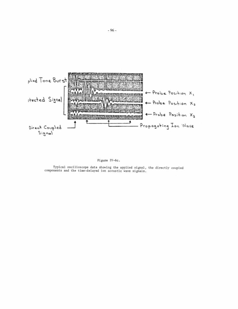
- 96 -

- 97 -

- 98 -

- 99 -

- 100 -his interferometer apparatus is summarized in Figure IV-7 along with a sample interferometer trace of

the ion acoustic signal h(x). Wavelengths and spatial damping rates are measured directly from such

recorder plots of h(x) vs. x. This diagnostic method holds the principal advantage of a long time

constant in the R-C filter, which averages out noise (uncorrelated signals) producing a good signal-to-

noise ratio.

4) Experimental Procedure

a) Tone burst: Set up the tone burst circuit of Figure IV-6 using an rf source to generate an

oscillating potential between the component chamber of the DP device.

i) Before activating the tone burst,

1) Monitor the ion distribution function to make sure no ion beam is present.

2) Double check the match of driver and target plasma potentials with Langmuir probes

positioned ~ 10 cm from the exciter grid.

3) Measure Ti to verify Ti << Te.

ii) Use the tone-burst generator to launch a wavetrain of sinusoidal oscillations. Observe the

propagation of the wavepacket with the disc probe (biased to collect electron saturation

current).

1) Measure δn/n by noting the density perturbation on a Langmuir trace or by biasing the

probe at a fixed potential above the plasma potential and monitoring the fluctuations in the

electron current δIe/Ie, which is proportional to δn/n, assuming there is no fluctuation of

temperature.

b) Measure δn/n by monitoring the ion wave signal at the floating potential,1 Vf, using the

capacitive probe of Appendix F.

3) Measure Vs, the plasma potential using a sampling technique. Collect the entire Langmuir

trace at a particular phase in the oscillating ion signal. Obtain Vs directly from the shape

of the Langmuir curve.

ii i) For a selected exciter frequency, find2

1) vp, the propagation velocity of the envelope of the wavepacket (group velocity), and

1 Convince yourself that if we assume the fluctuation of the floating potential is the same asthe fluctuating plasma potential, then

δn/n _ eδVs/KTe _ eδVf/KTe

Check this relation for several values of δn and Vf.

2 Both phase and group velocities are computed by displaying the applied exciter gridsignal and the received probe signal on the same scope trace and noting the time delayof corresponding features of the wave form as a function of the axial distance betweenthe receiving probe and separation grid.

- 101 -2) vg, the propagation velocity of a given peak within the wavepacket. Whenever this traveling

peak shifts phase (position) within the propagating packet, vp ≠ vg (dispersive wave

propagation).

iv) Check the parametric dependence of the signal investigated in step

iii):

1) Is damping getting stronger as ω approaches ωpi?

2) Compute the ion acoustic speed Cs by measuring Te in the target plasma with the Langmuir

probe. Does this value agree with the experimentally measured speed?

v) Carry out step iii) over as wide a frequency range as possible so that you can plot

1) ω vs. kr, the dispersion relationship, and

2) ω vs. δ/λ, where δ/λ is the spatial damping rate of the ion acoustic wave.

vi) Repeat the procedure in step v) for several different neutral pressure settings.

b) Interferometer: Set up the interferometer circuit as shown in Figure IV-7a. Again verify

that no ion beam is present and record interferometer traces with the continuous signal applied to the

exciter for a wide range of frequencies. Using this technique, replot the dispersion relation, ω vs. kr,

and the spatial damping dependence, ω vs. δ/λ, for several neutral pressure settings. Record any

irregular patterns in the waveforms and attempt to interpret your data in terms of more than one mode

propagating in the plasma (see Appendices B and E).

Appendix A: Landau Damping of Ion Acoustic Waves

1) General Dispersion Relation

We shall describe a more detailed theory of ion acoustic waves which includes the boundary

conditions at the excitation source. Ion dynamics will be included in this treatment to describe the

collisionless damping of ion waves.

In most experiments on ion acoustic waves, the frequency is much less than the electron-

electron collision frequency but greater than the ion-ion collision frequency. We shall therefore follow

the analysis of Jensen8 in treating the electrons as a fluid but shall describe the ions by a collisionless

Boltzmann equation in the manner of Fried and Gould.3 The electrons are characterized by an average

electron density ne, and average velocity ve, and isotropic pressure Pe. The equation of motion for

electrons is

nmdvdt

= neE p

xe e− ∂

∂(A-1)

where Pe = nKTe and E is the total electric field present at x at time t. The ions are described by a

velocity distribution function fi satisfying the one-dimensional collisionless Boltzmann equation

i i i idfdt

= ft

+ v f + eEM

fv

= 0.∂∂

∂∂

∂∂x

(A-2)

- 102 -A separate theoretical analysis10 has shown that axially propagating ion acoustic waves are

insensitive to radial boundary conditions because the strong shielding by electrons greatly reduces the

influence of electric fields at the boundary on the central propagating region. A one-dimensional

analysis should provide a reasonably good description of the propagation of ion acoustic waves.

We shall linearize (A-l) and (A-2) by letting

n = n0 + n1(x,t)

and

fi(x,v,t) = f0i(v) + f1i(x,v,t),

where foi(v) is the Maxwellian ion velocity distribution function. Since no external electric fields are

applied to the plasma volume (except at the exciter, located on the x = 0 boundary) the total electric field

E is just the self-consistent field due to the separation of the local plasma charges,

E = E1 (x,t).

Neglecting electron inertia (m/M << 1) and assuming isothermal conditions in equation (A-l) and

linearizing both equation (A-l) ant (A-2), one obtains

0 1 en eE KTn≈ ∂

∂1

x(A-3)

∂∂

ν ∂ ∂∂ν

ft

fa

eEM

fi i i1 1 1 0 = + =x

(A-4)

Next, Fourier analyze ant Laplace transform each of the first order terms in (A-3) and (A-4) into (k,ω)

space, as in the following steps, which involve integrations by parts:

- 103 -

dt dxn x t

xe dt e n x t e

o

i kx t i t ikx ,

, ∂∂

ω ω11 0

( ) = ( )∞

−∞

∞ − −( )−∞

∞ − ∞∫∫ ∫ dx ik n (x, t) e ikx− −

∞−∫ ( )

0 1

= dt n (0, t) e + ikn (k, )i t −−∞

∞

∫ 1 1ω ω

dt dx f (x, , t)

t e = dt

f (k,v, t)t

ei(kx t) i t

−∞

∞ ∞− −

−∞

∞

∫ ∫ ∫∂∂

∂∂0

1 1ν ω ω

= f (k,v, t) e dt i f (k,v, t) e1

i t1

i tω ωω

1 244 34 4 −∞

∞

−−∞∞

∫ ⇑ = 0 (See footnote 1)

= i f (k,v, ).− ω ω1

Solving the Fourier and Laplace, transformed versions of (A-3) and (A-4) for n1(k,ω) and f1i(k,v,ω),

respectively, produces

1o

en (k, ) =

in eE (k, )

kKT

iq( )k

ω ω ω1 − (A-5)

and

f (k,v, ) = i

kv eE (k, )

Mf (v)

v vg ( ,v) ,i

1 0ii1 ω

ωω ω

( )−∂

∂

(A-6)

where

q( ) dt n (0, t) ei tω ω≡−∞

∞

∫ 1

and

g( ,v) dt f (0,v, t) e .i tω ω≡−∞

∞

∫ 1

Note that n1(0,t) and f1 (0,v,t) are the boundary values of the electron and ion perturbations at the exciter

1 This term is zero because f (k,v,-∞) = 0 and the excitation is turned on very slowly at t

> -∞; there is a very small positive imaginary frequency component in ω = ωr + iδ suchthat the entire term vanishes at t = +∞.

- 104 -(x=0), and q(ω) and g(ω,v) are their respective Fourier transforms.

The Poisson's equation,

∂∂

− −

−∞

∞

∫1i o i

Ex

= 4 e(n n ) = 4 e dv n f (x,v, t) n (x, t) ,π π1 1 1 1 (A-7)

can also be Fourier-Laplace transformed to give

1 1 0 1i 1ikE (k, ) E (0, ) = 4 e dv n f (k,v, ) n (k, ) ,ω ω π ω ω−

−∞

∞

∫ (A-8)

where E (0,ω) is the field at the exciter grid (x = 0). Substituting (A-6) and (A-8) into (A-7) yields an

expression for the total electric field in the plasma

1 1iE (k, ) =

1ik (k, )

E (0, ) + 4 e vg ( ,v) dvi(kv )

q( )ik

ωε ω

ω π ωω

ω∞∞

∫ −−

(A-9)

Source Perturbed ion Electron density

electric distribution at perturbation

field source at source

where ε(k,ω) is defined as the dielectric constant for longitudinal waves, which describes the collective

response of the plasma to excitations of frequency ω and wave number k

ε ω πω ν

πk

n eMk

f v dvk

n ek Kt

o oi o

e

, ( )

©

( ) = +−

+−∞

∞

∫14 42

2

2

2 (A-10)

= +−

+−∞

∞

∫ ( )

©

12

2

2

2

ω ν νω ν

pi oi De

kf d

kkk

. * (A-11)

ion contribution electron contribution

The contribution of electrons (kDe2/k2) to shielding is large (since k << kDe under most experimental

conditions), as is expected from their high degree of mobility.

As indicated by the form of (A-9), the dominant contributions to the total plasma (wave) electric

field come from the set of ω's and k's which satisfy the dispersion relation ε(k,ω) = 0. The solution

to ε(k,ω) = 0 contains terms similar to those already derived in the fluid theory (equation 8 of Chapter

IV), plus an additional, imaginary part, which depends on the shape of the ion distribution function

foi(v) and pertains to wave damping.

- 105 -To see this dependence, let us solve for the roots (zeros) of the dispersion relation ε(k,ω) = 0

for a case of experimental interest, Te >> Ti, and ai << ω/k << ae, consistent with temperatures typically

observed in the DP device. first, rewrite the ion contribution to (A-11), which is an integration along

the real axis, using the identity

1/k v

= P1

/k v + i ( /k v)

ω ωπδ ω

(A-12)

where P denotes the Cauchy principal value and δ the delta function. Substitution of (A-12) into (A-

11) gives us a more explicit expression of the dielectric constant:

ε ωω ν ν

ω νπ

ωωk

kP

f dk

ik

f kkk

pi oi pioi

De, ( )

( ) ©

©( ) = +−

− +−∞

∞

∫12

2

2

2

2

2 (A-13)

valid for small damping ki << kr. Solving for ε(k,ω) = 0 using the relation

Pf d

k k

KTMk

oi

i

( )

© ν ν

ω ν ω ω−= − +

−∞

∞

∫ 11

3

2 2 2 2

we obtain analytic expressions for the real and imaginary wavenumbers kr and ki:

2

r

pi3KT

M k

k kk

1 + i

r De

ωω ω

2

2 12 2

2 2≅

+

or2

r

e i e

r Dek KT

M(1 + 3T / T )1 + k /k

ω2 2 2≅ (A-14)

and

The phase velocity calculated from the kinetic theory essentially agrees with the result of the fluid

theory (equation 8 of Chapter IV), since the wave motion is carried on by the main plasma moving as

a whole. The new result of the kinetic treatment lies in the imaginary wave number ki which describes

the contribution of the resonant particles traveling at the wave phase velocity. For a Maxwellian plasma

foi(v) = π-1/2 ai-1 Exp (-v2/ai

2),

- 106 -

i1/2

i

pi2

e

i

e

i

2

pi

i

ek =

2 a

T

TT2T

1 1 + 3TT

π ω ω

ωω

ω Exp

2

2

(A-15)

and the attenuation distance normalized to one wavelength is:

δλ π

ωω

π

ωω

= 1

2

k

k

r

i

TT

T

T

T

Ti

ee

i pi

i

e

pi

≅( ) −

+

−

3 2

31 1

3

2

2

2

3 2 12

2

1 2

Exp

(A-16)

where the approximation 1

1 + k /k = 1 /

2De

2pi2

2ω ω has been used.

- 107 - Appendix B: Collective and Free-streaming Contributions to Propagating Ion Acoustic Waves

When a grid is used to produce a local density perturbation and thereby launch an ion acoustic

wave, particles near the grid are accelerated and a perturbation on the velocity distribution function is

produced. This perturbation is carried by particles free-streaming contribution. When these particles

are collected by the detecting probe, their modulated velocity distribution makes a contribution to the

probe signal. This is called the free-streaming contribution to distinguish it from the collective plasma

behavior in ion acoustic waves derived in a homogeneous plasma. In the following we shall discuss

the collective and free-streaming behaviors in an experimental situation and their relative importance.

It is possible to distinguish one contribution from another through a systematic variation of plasma

parameters such as Te, Ti, n, the concentration of lighter ions, etc. This series of tests is summarized

in a table at the end of this appendix.

1) Free-streaming Ions and Spatial Landau Damping

In the laboratory, ion waves are detected by either collecting ions by a probe or energy analyzer,

or by monitoring the wave electric field by an electron beam diagnostic technique or a high impedance

probe. As explained below, each detection method emphasizes different aspects of ion waves. First,

we shall consider a method in which ion flux is detected.

a) Detection of ion flux: If the receiving probe is biased negatively to detect ion flux, J1, the

spatial variation of the detected signal is obtained via the inverse transform of the spatial Fourier

spectrum of the current:

J (x, ) = 1

2 dk J (k, ) e =

12

dk dv vf (k, ,v) e ,c

ikx

cli

ikx1 1ω

πω

πω∫ ∫ ∫−∞

∞

where c denotes the appropriate contour of integration in k space from the inverse Laplace transform.

Using the expression of f1i(k,ω,v) from equation (A-6), we obtain two types of contributions to the

current:

J xi

dvdk

kv

eM

E K f ei

dvvdk

kg eoi

ikxc

i collective term

iikx

c

ii free strea g term

1 12 2,

,

± , ©

) ) min

ωπ ω ω

π ων

ω νν( ) =−

( ) −

( )−∞∞

( ) −∞∞

−

∫ ∫ ∫ ∫1 24 4 4 4 4 4 4 4 34 4 4 4 4 4 4 4 11 24 4 4 4 44 34 4 4 4 4 4

(B-1)

i) Collective term: spatial Landau damping. In the collective term, the wave electric field E1 accelerates

the ions, ant together with the gradient of the ion distribution function produces and ion flow in the

velocity space. Integration over the entire velocity range - ∞ < v < ∞ sums up the contribution of ion

flow at each velocity to the overall ion flux. The collective effects are contained in the dielectric constant

term ε(k,ω) of the expression for the self-consistent field E (k,ω), as given in equation (A-9).

- 108 -The collective term is calculated by substituting (A-9) into (B-1)

and performing the integration over complex k space:

J collective E dviveM

f

k

Exp ik

k

x oi

k

res

res

Type A

res

1 12

0 ,( , )©

ω ων

∂ε ∂ ν ω= ( )

( ) ( )−

−∞∞

∫x

kres

6 74 4 4 4 44 84 4 4 4 4 4

+( )

−∞∞

∫ dviveM

f Exp iw

xoi

Type B

©

,

νν

ωε ων

ν1 24 4 4 4 4 4 34 4 4 4 4 4

+ similar terms with E(0,ω) replaced by vg(o, ,v) dvi(kv omegta)

ω−∞∞

∫+ similar terms with E(0,ω) replaced by q(0,ω). (B-2)

Here each boundary condition at x = 0[E1(0,ω), g(0,ω,v), and q(0,ω)] is propagated toward the detector

with a spatial phase Exp [ikresx], where kres is determined from the dominant root of ε(ω,k) = 0. This

behavior is represented by the type A terms in equation (B-2) and corresponds to the wave-particle

interaction proposed by Landau. A second spatial behavior Exp [ikeffx] is obtained from the integration

of the type B terms. It is similar to the phase mixing process to be discussed below except for the

plasma shielding term 1( /v,v)ε ω in the integrand.

Let us now consider the physical picture of free-streaming and phase-mixing processes. We

shall present an x-t diagram which illustrates the free-streaming behavior of the perturbed particle

distribution at the boundary. A simple argument gives a good estimate of the effective attenuation

distance x = (kerr)-1 due to phase-mixing among particles traveling at different velocities.

Consider an idealized grid which acts as a gate that either lets particles go through or absorbs

them completely. In Figure IV B-1, the grid located at x = 0 allows short bursts of particles to pass

through at intervals of τ. The lowest harmonic of this modulation corresponds to the frequency of our

exciter. The response of the receiver which detects ion flux I(t) as shown on the right is obtained by

an integration over velocity, i.e., I(t) = q vf(v) dv .−∞∞

∫ The velocity spread causes particles to

overtake one another or phase mix resulting in a loss of the original oscillating signal. An estimate of

the effective attenuation distance x0 at which phase mixing begins to occur is made by computing the

- 109 -time ∆τ required by the fastest ion (velocity v2) to overtake the slowest ion (velocity v1) of a previous

cycle. Referring to Figure IV B-!:

v2∆τ = v1 (τ + ∆τ) = x0.

This gives

∆∆ ∆

∆∆ ∆

τ νν

τ ν νν

τ ν νν

τ νν

πω

= x = = ( /2)

21

01 2 m

2 2m2

∧ _

where

m1 2

2 1 = +

2, = ν ν ν ν ν ν∆

or

.v

v

v2 = k

mmi

∆πω

(B-3)

- 110 - smaller the attenuation distance x0. As the frequency increases or the period shortens, the phase

mixing occurs over a shorter distance as expected. If vm is replaced by the thermal velocity ai and

assuming a velocity spread ∆v _ ai/2 then ki _ ω/4πai.

ii) Free-streaming term in the detection of ion flux. Returning to (B-1) we note that the second term

describes how a perturbation of the velocity distribution function at the exciter, g(x = 0,ω,v), propagates

out from the source. If the perturbed ion distribution g(ω,v) can be assumed to be Maxwellian, the free-

streaming term in equation (B-1) takes on the following form:

1 freestreami

2/3i

2/3J (x, ) (x

a) [ ( x/ a ) (1 i 3)].ω ω ω∝ Exp (B-4)

The above expression gives an effective decay constant ki _ ω/ai, which is similar to the result derived

from our physical model.

- 111 -

- 112 -

b) Detection of wave electric field E1(x,ω): If the fluctuation of plasma potential is monitored

by a probe technique or the wave electric field is directly measured by an electron beam method, the

detected quantity expressed in terms of the wave electric field E1(x,w) is just the spatial transform of

equation (A-9):

1c

1ikxE (x, ) =

12

dk E (k, ) eωπ

ω∫

= 1

2 dk [

E (0, ) + 4 e[ dv ]

ik (k, )]e .

c

1g (0, ,v)i(k /v

q(0, )ik

ikx

i

π

ω π

ε ω

ωω

ω

∫∫∞

∞

In using the residue theorem to evaluate this integral, we notice that there are again two kinds of poles,

a "free-streaming" pole at k = ω/v and a "collective" pole kres derived from the solution to ε(k,ω) = 0.

Summing these residues gives

1res

res k | (0, ) + 4 e

( ,v) dv

i( /v)

q( )E (x, ) =

[ik x]

kE

gk ikresk

1i

res resω ε ω π

ωω

ωExp∂∂

−∞

∞∫

i4 e v dv g ( ,v) e ( /v)x

( /v,v)i

i−

−∞∞∫π

ω ωωε ω

(B-5)

The first bracket contains the boundary conditions of the electric field, perturbed ion

distribution function and perturbed electron density, which propagate toward the electric field detector

with the spatial phase variation Exp [ikresx]; the last term of (B-5) is the contribution of the perturbed

ion flux generated at the exciter; those particles with a given free-streaming velocity v propagate with

an equivalent wavenumber k = ω/v. Summation over the entire velocity distribution taking the electron

shielding into account through the dielectric constant ε(ω/v,v) gives the total contribution of the free-

streaming ions to the wave field.

An estimate of the relative importance of the collective contribution and the free-streaming

contribution can be made. The former decays as Exp [-kix] ( where ki = Im kres) while the latter

approximately as Exp [-(ω/ai)x]. For our experimental conditions of high electron temperatures Te/Ti

>> 1 and a correspondingly high phase velocity, the Landau damping is weak for ω << ωpi and ki ≡ Im

kres << ω/ai. The collective behavior therefore dominates at distances x > ai/ω. Since the wavelength of

ion acoustic waves is given by:

λ πω ω

= 2 a (TT

ai e

i

i

>>1 2

we can safely state that at distances beyond one wavelength from the source the collective behavior

- 113 -makes the dominant contribution to the detected wave electric field.

2) Pseudo-ion waves

These are wave-like signals detected by the receiver probe, which are ion bursts emitted at

regular intervals by an excitation grid driven to large amplitudes (eφ0/KTe >> 1 where φ0 is the

oscillating potential of the grid with respect to the surrounding plasma).

Consider an exciter grid located at x = 0 with a typical sheath thickness of 20 λD in Figure IV

8-2. Particles at thermal velocities (KTi/M)1/2 enter the sheath region from below and are accelerated

if they encounter the correct phase of the oscillating electric field E(t) = E0 cos ωt. The trajectories of

certain particles are altered in such a way that upon crossing the grid they are further accelerated to a

maximum velocity v0 which can be estimated as follows:

12

Mv 2eo 02 ≤ φ

or

ν φo 0 e1/2

e1/2 2(e / KT ) (KT /M)≤

We note that only at a particular phase of the cycle are particles accelerated to the maximum velocity

v0 proportional to (eφ0/KTe)1/2. These fast ions can become the dominant contribution to a probe biased

to collect ion flux. As can be easily verified in the diagram, there is an associated wavelength λ =

2πv0/ω. Unlike ion acoustic waves, the wavelength and hence the phase velocity of this pseudo wave

are strongly dependent on the exciter amplitude. The attenuation arises from phase mixing among the

bursts in a manner similar to that in the free-streaming contribution discussed previously for ion

acoustic waves.

3) Experimental Differentiations Between Collective and Free-streaming Contributions to Ion

Acoustic Waves

These two major contributions to ion acoustic waves can be distinguished from each other by an

examination of their dependence on various plasma parameters. By "free-streaming contributions" we

imply both the small amplitude free-streaming mode and the large amplitude pseudo ion waves For

example, for frequencies near ωpi, ion acoustic waves are strongly Landau damped, while ballistic

contributions and pseudo waves are easily observed for ω ~ ωpi. Another important distinction is their

parametric dependence on the electron temperature. The collective behavior driven by electron

pressures is more sensitively dependent on Te than the free-streaming behavior.

As we shall discuss in Volume III, when there is an electron drift of velocity comparable to the

ion acoustic phase velocity, only the collective mode can grow spatially there are more electrons

traveling faster than the wave than those traveling slower. The free-streaming contribution and the

pseudo ion wave do not undergo any spatial growth at all as they are not dependent on resonant

particles. This is an example of using an external free energy source to distinguish the collective ant

- 114 -free-streaming contributions, These differences in parametric dependence are summarized in Table IV

B-l.

- 115 -TABLE IV B-1

Experimental differentiation between collective and free-streaming behaviors.

ION ACOUSTIC WAVES

Collective ContributionFree-streaming Contributi

Description Ion density perturbation driven by electricfield, which is caused by chargeseparation between ions and electrons.

Individual particles in perturbed idistribution f1(ν) free-stream at threspective velocities from the southe exciter

Dependence on Te/TiLandau damping (wave particleinteraction) decreases with increasing

Te/Ti. Vp = 3 1 2KT KT

Mi e+

.

δλ does not depend on Ti or Te/T

Apparent vp increases with Ti;

vp = 2

3 2

1 3

ax

aii

ω

.

φ Amplitude of exciter Vp independent of φ in linear regime Vp is independent of φ.

Effects of ion-ion collisions Landau damping is decreased, becauseion-ion collisions prevent wave-particleinteraction.

Phase-mixing increases with νii.

Addition of impurity ions traveling at vph. Landau damping increased drastically. Negligible change in damping.

Frequency range. Waves cannot be observed near ωpibecause of severe Landau damping.

Observable near and above ωpi

Methods of detections. Best observed if electric fields aredetected.

Best observed if ion current is de

δλ = damping distance normalized to the wavelenght

Vp = phase velocity

- 116 -Appendix C: Damping of Ion Acoustic Waves in Presence of a Small Amount of Light Ions12

The collisionless interactions between ions and ion acoustic waves can be increased by the

addition of a lighter ion species whose thermal velocity is close to the wave phase velocity in other

words, the population of resonant ions can be controlled by varying the amount of light ions. If the

amount of light ions is small, the wave phase velocity remains virtually the same, because the wave is

carried by the bulk plasma. Theoretically the only addition to the dielectric constant in equation (A-13)

is an imaginary term due to the newly added resonant ions: -iπ (ω* pi2/k2) f* oi(ω/k) where the *

quantities refer to the new species. Carrying out the same procedure as in Appendix A, we find

kk

f knn

MM

f kipi

roi r oi r= − ( ) + ( )

*

*

©© *πωω ω

2

2

contribution of light ions

If both the background ions and the light species have Maxwellian distributions and are at the same

temperature, then

i1/2

i

pi2

2e

i

e

i

2

pi2

e

i

2

pi2k =

2 aTT

12

TT

1 + n *n

M *M

12

TT

M *M

1

π ω ω

ωωω

ωω

Exp Exp

−

1 2

contribution of light ions

The mass dependence in the exponential term can make the contribution of light ions to

damping comparable to the background ions. For example, the addition of 3% Helium to an Argon

plasma of Te/Ti _ 10 would approximately double the spatial damping rate. A qualitative picture of the

two ion distributions together with the phase velocity is depicted in Figure IV C-l, which shows a larger

number of lighter ions traveling near the wave velocity.

- 117 -

- 118 -Appendix D: Ion Acoustic Shocks

This section deals with a nonlinear state13,14 which develops when the amplitudes of density or

potential perturbations become large (eφ/KTe or ∆n/n0 ≥ 10%). It can be looked upon as a propagating

discontinuity which separates two regions of different densities, potentials and temperatures. The

propagating speed of this shock, vs, is always greater than vp of an ion acoustic wave and a Mach

number Μ = vs/vp > 1 is associated with a shock of a given amplitude. We shall first point out the

nonlinearity in a simple fluid treatment which is supplemented by a kinetic argument showing the

importance of particle reflections from the shock front.

1) Theory

a) Fluid equations with nonlinear terms: In obtaining the linear dispersion [equation (3)] for

ion acoustic waves using the fluid approximation, we have neglected the nonlinear term ivxv i∂

∂ in

equation (1), the equation of motion for ions the inclusion of this term together with the equation of

motion for electrons gives:

i ii

is

ddt

= t

+ x

= 1n

Cnx

ν ν ν ν∂∂

∂∂

∂∂

(D-1)

for Te >> Ti and negligible electron inertia at ion frequencies.

When the fluid density and velocity n, vi are expressed as function of a single variable, u = x/t,

a simple relation exists between them. Let us rewrite (D-l) in terms of this new variable u using the

transformations ∂∂∂∂x

1t , = = d

du tut

ddu :

nuddu

+ nddu

+ Cdndu

= 0ii

is2ν ν ν (D-2)

or

(u )d = Cdnn

.i i sν ν 2 (D-3)

A similar analysis of the equation of continuity for ions gives:

i id = (u )dnn

.ν ν (D-4)

Equations (D-3) and (D-4) have compatible solutions if u = vi ± Cs is used in (D-2), and after

integration one obtains:

i s

0s

e = C

n

n = C

eK T

.νφ

ln (D-5)

The Boltzmann distribution n = n0 Exp (ef/KTe) has been used in the above expression. Equation (D-

- 119 -5) states that the fluid velocity is proportional to the plasma potential or to ln (n/n0); in other words, the

larger is the potential or density perturbation, the faster the local fluid element. As shown in Figure IV

D-1a, a large amplitude ion wave can steepen to form a sharp front because the higher density or

potential region travels faster.

ii) Second case: u = vi - Cs. The student can verify that this case does not give rise to a

shock formation; instead a rarefaction wave is developed.

The student will observe in the laboratory that ion acoustic shocks maintain

approximately constant shapes only over a rather limited distance on account of charge

exchange collisions, plasma inhomogeneities, and other processes.

- 120 -b) Ion reflections from the shock front: The plasma in which a shock travels is composed

of ions of a range of velocities. Ions are reflected from the shock front if their relative velocities, v, with

respect to the shock, are small enough such that 1/2 Mv2 £ qf0, where f0 is the potential jump in the

shock, Figure IV D-1. Let us consider a frame moving with the shock speed vs in which the shock

front appears stationary. Those background ions with v < vs in front of the shock will appear flowing

toward the shock front, Figure IV D-1a, with a relative speed v' = vs - v. The ion distribution f(v') in

the moving frame is depicted fin Figure IV D-1b which shows the range of velocities of ions to be

reflected: 0 < v' < (2qf0/M)1/2. After reflection, ions move in a direction away from the shock front

as shown in Figure IV D-1c. In the laboratory frame, these ions travel faster than the shock by the

same amount as they were traveling slower before reflection. In the experiment, the student is expected

to observe a density bump at the foot of the shock front as in Figure IV D-1c. An analysis of the

velocity distribution at this bump will show a beam-like distribution consisting of faster ions. The

percentage of fast ions observed experimentally could be checked against a theoretical estimate which

integrates over the shaded velocity range of Figure IV D-lb, once the ion temperature and the shock

speed vs are measured. Since the number of reflected particles is a sensitive function of the location

of vs ≅ Μ(KTe/M)1/2 with respect to the ion distribution, another experimental check of the theory can

be made by measuring the number of reflected particles as a function of Te /Ti.

c) Consequences of reflected ions: Ion reflections from the shock front result in a net

extraction of energy from the propagating front. In a plasma with infrequent collision, this reflection

process is the dominant dissipation process which leads to the formation of shocks (see the Sagdeev

potential of Chapter 8 in Chen's book, "Introduction to Plasma Physics".)

Secondly, the beam-like distribution that is formed by ion reflections from the shock front can

give rise to ion acoustic instabilities, similar to those in ion beam-plasma interactions. Ion wave

turbulence has indeed been observed ln the shock front as a result of such interactions.14

- 121 -

- 122 -

- 123 -

- 124 -

- 125 -

- 126 -2) Experiment

Adapt the tone-burst configuration outlined in Figure IV-6 to set-up diagrammed in Figure IV

D-2a. A long (~ 100 µsec) pulse is applied between the two chambers. The capacitor C0 across the

output of the pulser increases the rise time of the pulse so that a more gradual steepening of the ion

acoustic disturbance can be observed. The following experiments are suggested.

a) Vary the amplitude of the applied pulse and observe the plasma response. Verify that for

small density perturbations the response is linear --that is, the launched ion acoustic pulse has

approximately the same shape as the applied pulse. How large does the density perturbation have to

be before the edge of the pulse begins to steepen? Observe the plasma response for several values of

initial density perturbations δn/n. Under the most optimum conditions, when the spatial steepening of

the shock front can be clearly seen, record the evolution by making several exposures on one film.

b) Launch a small amplitude, linear ion acoustic tone burst and measure vp. Then launch a

shock and measure the shock speed, vs, as a function of the shock density perturbation. Plot vs vs. δn/n.

find out the range of Mach numbers, Μ = vs/Cs, that can be obtained in the experiment.

c) Observe the bump in front of the shock. record the characteristics of the shock, as a

function of Te/Ti, giving special attention to the bump just ahead of the shock. Use an ion energy

analyzer and a sampling scope to record the distribution function at the location of this bump. Does

the number of reflected particles and the shape of the distribution agree with the theoretical expectation?

Be as quantitative as you can.

d) Record the characteristics of the wave-train trailing behind the shock front. Study Chapter

8 in Reference 2 and explain the wave train in terms of the Sagdeev potential.

- 127 -

- 128 -

- 129 -

Reference

1. L. Tonks and I. Langmuir, Phys. Rev. 33, 195 (1929).

2. J. D. Jackson, J. Nucl. Energy: Pt. Cl, 171 (1960); I. B. Berstein, E. A. Frieman, R. M. Kulsrud,

and M. N. Rosenbluth, Phys. Fluids 3, 136 (1960); E. A. Jackson, Phys. Fluids 3, 786 (1960);

I. B. Bernstein and R. M. Kulsrud, Phys. Fluids 3, 937 (1960).

3. B. D. Fried and R. W. Gould, Phys. Fluids 4, 139 (1961).

4. T. H. Stix, The Theory of Plasma Waves (McGraw-Hill Book Company, Inc., New York 1862),

p. 132.

5. L. Landau, J. Phys. (USSR) 10, 25 (1946).

6. A. Y. Wong, R. W. Motley and N. D'Angelo, Phys. Rev. 133, A 436 (1964).

7. G. Sessler and G. Pearson, Phys. Rev. 162, 110 (1967).

8. V. O. jensen, Risö Rept. No. 54, Risö, Roskilde, Denmark, 1962 (unpublished).

9. The collisionless contribution by electron is treated theoretically in R. W. Gould Phys. Rev. 136,

A991 (1964); and experimentally by A. Y. Wong, Phys. Rev. Lett. 14, 252 (1965).

10. A. Y. Wong, Phys. Fluids 2, 1261 (1966).

11. B. D. Fried and S. D. Conte, The Plasma Dispersion Function, (Acad. Press, New York, 1961).

12. I. Alexeff, W. Jones, and D. Montgomery, Phys. Rev. Lett. 19, 422 (1967).

13. R. Taylor, H. Ikezi and D. Baker, Phys. Rev. Lett. 24, 206 (1970).

14. A. Wong and R. Means, Phys. Rev. Lett. 27, 973 (1971).

15. T. E. Stringer, Plasma Physics 6, 267 (1964).

16. B. D. Fried and A. Y. Wong, Phys. Fluids 9, 1084 (1966).

17. N. Sato, H. Sugai, R. Hatakeyama, Phys. Rev. Lett. 34, 931 (1975).

18. D. R. Baker, Phys. Fluids 16, 1730 (1973).

Appendix E: Ion Beam-Plasma Interactions in a One Dimensional Plasma

We have seen that in a magnetic field free plasma, with Te >> Ti, there exists a low frequency (ω< ωpi) normal mode, the ion acoustic wave, with phase velocity

ps

2D

s e1/2 = /k = C

1 + k, C (KT /M ) .ν ω

λ= ±

( )≡

2 1 2

If a cold ion beam with velocity vb is injected into such a plasma, we find, in addition to the background

ion modes, two ion beam modes. The dispersion relation for the four low frequency modes is given

by the fluid theory as

ε ωω

ω

ωω λ

( ,k) = 1 ( kv )

+ 1

k = 0pi

2pb

b2 2

D

2 2

2− (E-1)

- 130 -or

1 + k nn

C n

n

C

(v v ) = 02

Di

e

s

p

b

e

s

p b2λ

ν2

2

2

2− (E-2)

Exercise: Obtain equation (E-l) by treating the plasma as a three fluid system with Ti = Tb = 0 and

proceeding in the spirit of the ion acoustic wave derivation given in Chapter IV.

The nature of the solutions of equation (E-2) will be discussed for two cases of interest, vb >> Cs, and

vb ~ Cs.

1) Case 1: v b >> C s

If the beam velocity is much greater than the sound speed, the beam and background ions are not

strongly coupled. The background ions support slightly modified ion acoustic waves and the berm

ions support ion acoustic waves whose phase velocities are shifted by the beam velocity. The velocity

distributions are sketched in Figure IV E-l.

For this case, approximate solutions to equation (E-2) may be obtained by making the

assumptions outlined above, to be justified a posteriori. A second order equation for the background

ion modes may be obtained from (E-2) by neglecting vp (<< vb) in the last (beam ion) term, yielding the

solutions:

pi e

1/2s

2De

e

s

b

sv = +(n / n ) C

1 + knbn

C

C

λν

22

2

1 2

= ± © (E-3)

To obtain approximate solutions for the beam modes, a simple transformation to the beam frame yields

an equation similar to (E-2) but with the roles of ni and nb interchanged. The solution is:

v vn / n C

1 + knn

Cp b

b e s

2D

i

e

s

b

−( ) = ± ( )

−

1 2

22

2

1 2

λν

(E-4)

We see that the background ion modes no longer propagate with speed Cs, but with reduced speed

Cs' ~ (ni/ne)1/2 Cs. The acoustic waves carried by the beam are similarly modified. A full kinetic

treatment of the problem reveals that all four modes are weakly damped by ion Landau damping

when Te >> Ti and vb >> cs.

- 131 -

- 132 -

- 133 -2) Case 2: v b ~ C s

When the beam velocity is approximately equal to the sound speed, the beam and background ions

are strongly coupled. An unstable ion wave grows by absorbing free-streaming energy from the beam

ions. This "ion-ion instability" is a member of the important class of electrostatic two stream

instabilities,15 which arise whenever a relative drift exists between two plasma components.

Figure IV E-2 illustrates typical results of a numerical solution of the ion beam plasma dispersion

relation derived from fluid theory, including the finite ion temperature. For vb > 2Cs, the fast and slow

beam modes and the background ion acoustic wave discussed under case 1 appear. For beam velocities

below about twice the sound speed, 0.7 Cs ≤ vb < 2Cs, the slow beam wave and the background wave

couple to form an unstable wave with a finite growth rate. The fast mode continues to exist in a stable

form.

The lower limit of vb _ 0.7 Cs for the instability is a finite ion temperature effect the system

becomes stable when the beam and background ions overlap sufficiently in velocity space. Below this

limit the fluid theory is no longer adequate for the coupled mode with phase velocities 0 < vp < vb

kinetic theories,2,16 which take into account wave particle interactions, show that this mode is strongly

Landau damped.

3) Experiment 1 - Observation of Beam Ion Acoustic Waves

In this experiment we shall observe the fast and slow beam waves discussed under Case 1 (vb

>> Cs) in the theory section. The double plasma device is adjusted to obtain a beam in the target

chamber, vb >> Cs, and small-amplitude test waves are launched by varying the potentials between

the two chambers or by applying modulation to the separation grid. This excitation launches both

fast and slow beam waves so the tone burst method (described earlier in the chapter) must be used

to separate the responses. The two modes, traveling with different velocities, will become separated

in space away from the excitation point.

We may compute the propagation distances for complete separation of the responses, referring

to Figure IV E-3. A tone burst of length τ occupies a spatial extent ∆x = vbτ.

The responses will be fully separated when the distances xf and xs travelled by the fast and

slow modes are separated by ∆x:

xf - xs = vbτwhich occurs in a time τ,

vft - vst = vbτ

t = v v

= 2(n /n ) C

b

f s

b

b e1/2

s

ν τ ν τ−

- 134 -

- 135 -

- 136 -

where the subscripts f and s refer to the fast and slow modes, respectively.

Thus the beam travels a distance

x = v t = 2(n /n ) C

.bb

b e1/2

s

ν τ2(E-5)

Examination of (E-5) reveals the optimum experimental conditions for the identification of the two

beam modes:

a) τ short: Use a tone burst of a few cycles try one or two cycles at 400 kHz, or even a pulse.

b) n b large: Adjust the source and target chambers to obtain the maxi-mum beam density.

c) v b small: Choose 3Cs ≤ vb ≤ 5Cs to satisfy our criterion of a fast beam.

The beam waves will be strongly damped if the beam is scattered by ion neutral collisions, so the

neutral pressure should be kept as low as possible, preferably below 10-4 torr.

An example of tone burst detection of fast and slow beam waves and the background ion

acoustic wave is shown in Figure IV E-4. Note that the beam waves are much more weakly damped

than the ion acoustic waves. The student should compare his beam wave observations with the ion

acoustic wave observations made in a previous experiment. Relate the damping rates to the

observed background and beam ion temperatures.

The two beam modes may also be observed by interferometry using our excitation signal as a

reference. The two waves, with wave numbers k1 and k2, form a spatial beat pattern.3,17

4) Experiment 2 - Ion-ion Two Stream Instability18 (vb _ Cs)

The purpose of this experiment is to study some of the characteristics of the ion-ion two

stream instability. Stability limits and growth rates will be determined by the test wave method.

The student should thoroughly understand the results of the ion acoustic wave and energy analyzer

experiments before attempting this experiment.

Set up the DP device for the interferometric observation of ion acoustic waves. A CW signal

source is used to apply an excitation to the separation grid. Position the energy analyzer about 3

cm from the separation grid and adjust the source chamber potential to obtain a beam of energy

about 10 V. Set the beam current to about one-tenth the background ion current by adjusting the

source and target chamber densities.

Now readjust the beam energy to zero by varying the potential of the anode and obtain the

propagation of an ion acoustic wave in the absence of a beam as a reference.

Apply a CW excitation signal at 1/3 the ion plasma frequency and obtain an interferometer

trace by moving the Langmuir probe (biased above the plasma potential) axially starting at the

separation grid. The excitation amplitude should be kept as small as possible to avoid nonlinear

- 137 -effects. An excitation amplitude of 10 - 500 mVpp should be sufficient. This interferometer trace

should indicate the presence of a damped ion acoustic wave.

Increase the beam energy in steps of 0.25 V or less taking an interferometer trace at each step.

The student should look for the smooth transition (as a function of beam energy) of the ion

acoustic wave to the fast beat wave (refer to Figure IV E-2) and for the appearance of the spatially

growing wave.1 Continue increasing the beam energy until the instability is no longer observed. An

example of interferometer traces in the range of beam energies 0 < Eb < 7 V is given in Figure IV E-

5.

Plot the observed phase velocities and the damping or growth rates as a function of beam

velocity. Compare your results to Figure IV E-2 or to the experimental or theoretical results

presented in references 16 and 18.

5) Other Suggested Experiments

a) Spontaneous noise behavior: In the absence of a test wave, spontaneous density

fluctuations in the unstable frequency range (ω ≤ ωpi) will grow in the direction of beam

propagation. Obtain unstable beam conditions and measure the spatial growth rate and saturation

amplitude of the noise by biasing the Langmuir probe above the plasma potential and measuring the

ac probe current fluctuations. If a spectrum analyzer is available, the frequency dependence of the

noise behavior may be studied.

c) Ion velocity distribution: As the unstable waves grow, absorbing energy from the beam, the

beam particles are slowed down. The beam spreads in velocity space and eventually

merges with the background ions, saturating the instability. Use the energy analyzer to

study the spatial development of the ion distribution as a function of distance from the

beam injection point (separation grid). Correlate the behavior of test waves or noise with

the modification of the distribution. Reference 18 is highly recommended in connection

with this experiment.

d)

1Note: The excitation amplitude should be substantially reduced when observing the unstable

wave to prevent nonlinear saturation of the wave and resulting erroneous measurementof the growth rate.

- 138 -

- 139 -

vk ep

22223+=ωω

( )T eexke >>φ

Chapter V. Electron Plasma Waves

1) Introduction The electron plasma density oscillation is one of the most fundamental excitations inplasmas. In the simplest approximation it is driven by electric fields caused by displacements ofelectrons from the background ion distribution. Although it is easy to derive this modetheoretically for uniform plasmas ( is the dispersion) the experimental verification of the simpletheoretical formulation is a rather difficult task. The electric field arising from the out-of-phasemotion between electrons and ions in electron plasma waves (hereafter referred to as EPW) issignificantly larger than that in ion acoustic waves in which ions andelectrons move in near synchronism. This electric field makes thewave characteristics very sensitive to the radial boundary conditions or how the E-field isterminated at the wall. Wave reflections at the wall set up radial modes which complicate thesubsequent analysis. Secondly, the collective behavior of electrons depends on the plasma density. Thepropagation of EPW is very sensitive to the density profile or any local density perturbation,created by probes for example. These considerations require a large plasma in which a gooddensity uniformity is maintained in the propagation region. In addition caution must beexercised in the excitation and detection of these waves since the probe sheath itself, a densityand potential inhomogeneity, might play a significant part in the data, again making a straightforward interpretation impossible. Special diagnostics, such as a collimated electron beam, areused to measure the absolute amplitude of these waves, as an independent check on theconventional probe diagnostics.

EPW can be excited along with free steaming modes at the excitation source. Electronsstreaming through a grid to which the excitation signal is applied can be modulated to form free-streaming modes which propagate at the streaming velocity. If the excitation signal is largebursts of electrons are generated at the grid similar to the ballistic mode discussed in Chapter IV.

The experiments described in this chapter are designed to excite the collective mode,commonly discussed in basic theories, while avoiding the other modes which can be excited atthe source. It is hoped that the experimental results thus achieved will be sufficiently universalin character to be relatively independent of the characteristics of the particular experimentaldevice used. In the following an experimental method is described which emphasizes theexcitation of the collective mode and which produces waves in a region many wavelengths fromthe exciter.

Our experimental method takes advantage of the fact that among the possible electronmodes which can be excited by the grid, only the collective mode can growspatially in the presence of the electron beam, Free-streaming and ballisticmodes decrease in amplitude as they move away from the source as a result of phase-mixingamong particles of different velocities; the spatial phase of each velocity class varies accordingto exp (i ϖ/ψξ). It will be shown that the most unstable waves have frequencies and wavenumbers near the intersection of the dispersion curves (Figure V-1) for uniform plasmas

( )222 /3 kmkTepe +=ωω and electron beams ( )Dkv=ω . for such spatially growing modes avery small excitation signal can be used and the detector placed well away from the exciter,thereby reducing the direct coupling between the exciter and receiver. In the plasma properwhere the density profile has the highest uniformity, we can measure the EPW wavelengths andamplitudes using the interferometry technique and compare the results with the predictions of thetheory of EPW in a spatially uniform plasma.

2) Theory of Electron Plasma Waves in the Presence of an Electron Beam

1 02 2

+ ( ) + ( ) =

−( )−∞

+∞

−( )−∞

+∞

∫ ∫ω

∂

∂ω

ω∂

∂ω

pe

e

b pe

b

k

kf

vdv

kvnn k

kf

vdv

kv

ε ω ω ωp D bb

pek kv ikvn

n,( ) − +[ ] =

2 2

The one dimensional dispersion relation governing the propagation of Electron PlasmaWaves (EPW) in a uniform plasma has been derived in many texts1 and given by

To treat growth or damping of EPW in the presence of an electron beam we must resortto kinetic theories which include the interaction of the beam with the waves. One such kineticdescription has been given by O'Neil and Malmberg2 who started with the one dimensionaldispersion relation for a beam-plasma (assuming stationary ions)

(1)

(1)

where fe and fb are the background and beam electron velocity distribution functions

respectively, ( )nnb / is the ratio of the beam and background plasma densities, and all first orderquantities are assumed to vary as exp [i (kx- ϖt)].

To proceed with this theory we assume a Maxwellian distribution for the backgroundelectrons and a Lorentzian distribution for the beam electrons3. Equation (1) then gives for ourdispersion relation

(2)

where ( )ωε ,kp is the background plasma dielectric function

ε ωω

ωppe

fe

vkk

k dv

kv,( ) = +

∂

∂

−( )−∞

+∞

∫12

and ≡Dv beam drift velocity, ≡bv beam thermal spread.

In the following we shall treat a variety of beam plasma interactions ranging from a veryfast beam with a relatively small thermal spread (cold beam) to a slow beam with a broadthermal spread (warm beam). In our discussion we will restrict ourselves to the weak beamlimit, ( )nnb / << 1. In this limit we can separately treat three cases according to equation (2):

(i) ( ) 1,0, >>+−≈ bDp vikkvk ωωε

11 CC hh eenn ,, FF .. ,, II nn tt rr oo dd uu cc tt ii oo nn tt oo PP ll aa ss mmaa PP hh yy ss ii cc ss ..

22 OO ''NNee ii ll aanndd MMaa llmmbbee rrgg ,, PPhhyyss .. FF lluu ii ddss 11 11 ,, 88 ((11996688)) ,, pp .. 11775566 ..

33 ff 00 == (( ee )) -- 11 eexxpp (( --vv22 // ee22 )) ,, ffvv == bb // [[ ((vv--vvDD )) 22 ++ bb

22 ]] -- 11

ω ω2 2 2 23= +pe ek v

0,1 <>> pp εε

(ii) ( ) ( ) 0,1, ≈+−>> bDp vikkvk ωωε

(iii) ( ) 0, ≈ωε kp and ( ) 0≈+− bD vikkvω

(i) If ( ) 0, ≈ωε kp and 1>>+− bD vikkvω , equation (2) describes an EPW propagatingin the background plasma according to the uniform plasma dispersion relation with phasevelocity ϖ/k very different from the beam drift velocity Dv . This wave is unaffected by thepresence of the electron grow since it does not couple to the free energy carried by the electronbeam.

(ii) If ε ωp D bk w and kv ikv( , ) | |≈ − + >>0 1, we have a beam mode traveling near thebeam velocity whose propagation characteristics are very different from the EPW in (i). Solvingequation (2) for k, we obtain

k

n

n

v vv iv

peb

p

D bD b=

±

+( )+

ω ωε1

1 2

2 2

/

( )

Writing

αε

≡

<<

n

nb

p

11

1 2/

, we have

k v

v

v

v vr D

pe b

D

D b

=

±

+ω

ω

ωα1

2 2( )

k v

v

v

v vi D

b

D

pe

D b

=

±

+ω

ω

ωα

( )2 2

for .

For our choice of notation on (exp [i(kx- ϖt)]) spatial growth of the waves occurs when ki < 0.

Thus the cold beam case v vb D/ ≈( )0 yields weakly growing waves with

k

k

n

ni

r

pe pe b

p

= −

= −

<<

ω

ωα

ω

ω ε

11

1 2/

.

(iii) We have seen that the two modes ε p ≈ 0 and ω − +( ) ≈kv ikvD b 0 taken separately either undergo damping or do not grow significantly. If we wish to excite a mode which is easily observedexperimentally we must look for a mode which exhibits strong growth. Such a modecorresponds to the third case, ε ωp D bkv ikv≈ − +( ) ≈0 0, where the phase velocity of the beam

v

v

n

n

v

vb

D b

e

D

62

2

1 3

/

mode matches the phase velocity of the EPW of the background plasma as depicted in Region Aof Figure V-1. The solution of the dispersion relation [equation (2)] for this case can be obtainedby Taylor expansion in the region A about the intersection point ( )oo k,ω , (see Appendix 1). Inthis derivation a dimensionless parameter s has been found useful in describing the entire rangefrom warm to cold beams.

S = scaled thermal speed =

The cold beam case is represented by s ≈ 0 and the warm beam case by s ≥ 0.For comparison the qualitative behaviors of the solutions of the dispersion relation for the

limiting cases of warm and cold beams s=2, s=0, have been plotted in Figure V-2. (s=2 isconsidered a limiting case since the numerical results are essentially unaltered when s exceedsthis value.) The regions where spatial growth takes place are cross hatched. The physicalsignificance of these two results will be explained in the following sections.

3) Physical Pictures of the Beam-Plasma InstabilityAlthough it is difficult to describe a physical picture which is generally applicable to the

beam plasma instability it is possible to understand the physical mechanism of the instability intwo limiting cases corresponding to cold and warm beams.

The parameter s which characterize the beam conditions can be varied in several ways.We will, however, concern ourselves with constant but small beam density 1/ <<nnb , constant

beam De vv / and assume that s has variations due only to changes in

the thermal spread, Db vv / . Warm Electron Beam

Figure V-2a summarizes graphically the numerical results obtained from the solution ofequation (2) for a warm beam. The warm beam-plasma instability corresponds to the picture ofinverse Landau damping. When a wave has a phase velocity pv less than the beam drift

velocity, Dv , there are more beam electrons with v > vp than with v < vp (since the beam

distribution function has a positive slope for v < Dv , see Figure V-3). There is a net transfer ofenergy from the beam to the wave which then grows. This situation is also described in figuresV-1 and V-2a: on the curve ( ) 0, =ωε kp

, points with oωω > correspond to waves with phase

velocity Dp vkv <= /ω which are calculated to be growing waves according to equation (2).

Cold Electron BeamFor a very cold electron beam we take the beam thermal spread 0=bv and write

equation (2) as

or

kv v

n n

kD

p

D

b

p

= ±( )

ω ω

ε ω/,

/1 2

Since the Fourier components of the electric field have been assumed to vary as exp [i (kx -ϖt)], spatial growth will occur if k has a negative imaginary part corresponding to ( ) 0, <kp ωε .

Referring to Figure V-4 we can understand the physical mechanism for the cold beam

ε ω ωp Db

pekvn

n−( ) =

2 2

plasma interaction as follows:In the beam frame beam electrons in a density trough will experience a stationary electric

field due to the bunched electrons on both sides of the trough. If there is no background plasmathe vacuum electric field, Evac, will be such that electrons in the trough feel a force F = -eEvacwhich is repulsive and tends to keep them in the trough. However, in the presence of abackground plasma characterized by the dielectric function pε the total field seen by the beam

electrons is pvacT EE ε/= . If pε is negative ET is opposite to Evac in direction the electrons areexpelled from a trough causing further bunching of electrons at each side of a given trough.Therefore, the initial perturbation on the beam grows under the condition that the dielectricfunction of the background plasma is negative.

4) Experimental ApparatusThe experimental apparatus used for the study of EPW is the double gridded double

plasma (D.P.) chamber as shown in figure V-5.In the D.P. device, the source and target plasmas are independently produced in separate

chambers by primary electron bombardment of a neutral gas. The potentials are arranged in sucha way as to cause the target plasma to be at a positive potential with respect to the source plasma.The target chamber wall and grid 2 are grounded. The source chamber grid (grid 1) is biasednegatively at -Vbias with respect to grid 2. This negative bias on grid 1 inhibits the flow ofelectrons from the source to the target chamber, thus permitting the establishment of twodifferent plasma potentials in the source and target plasmas. The wall of the source chamber isnot anchored to any external DC potential; it adopts a negative potential with respect to thesource plasma potential because electrons are lost to the wall at a faster rate than ions. Thesource plasma then has a positive potential with respect to the wall and grid 1 but is negativewith respect to the target plasma. The resulting potential profile as depicted in Figure V-5baccelerates electrons from point A to point B, creating an electron beam for our experiment. Itshould be pointed out that only the tail of the source electron distribution can overcome thenegative potential barrier at A and is then accelerated in the region between the grids to B.

The drift velocity, Dv , of the beam is controlled by varying the voltage bias between the

grids. The ratio nnb / can be changed either by varying the target plasma density, n, or by

indirectly varying the beam density, bn , through variations in the source plasma density. The

thermal spread bv of the beam is controlled by both the source temperature and the drift velocity(or the bias Vbias). The reduction of the thermal spread with increased drift velocity is the sameas described in Appendix A of Chapter II.

Typical operating parameters are: no ≈108 - 109 cm-3, ve ~ (KTe/m)1/2 ~ 6 _ 107

cm/sec, nnb / ~(5-10) % and eD vv / ~(5-10), Db vv / ~10-50%. The plasma frequency lies in theconvenient range of 100-300 MHz where the standard laboratory test equipment is available.

As we have seen in the physical pictures, the beam-plasma instability is initiated bymodulating the beam density and thereby creating the associated spatially oscillating potentialalong the beam. Experimentally this is achieved by applying an oscillating voltage of the desirefrequency in addition to the DC bias between the grids. The RF and DC voltages areindependently applied to a grid signal mixer (GSM) which in turn applies the combined signal tothe grid. The function of the GSM is to provide isolation between the DC and RF supplies. Thetypical applied RF signal strength is 0.1 V peak-to-peak and in general should be as small aspossible in order to avoid ballistic modes produced at the excitation grid.

5) Diagnostics Three diagnostics are used in this study of EPW. They are the two-sided Langmuir

probe, the RF pickup probe, and the diagnostic electron beam. The two-sided Langmuir probeconsists of two, identical, separate metal discs (typically 5 mm diam., 0.5 mm thick) placed backto back in the target plasma (see Figure V-6a). These discs are oriented such that one disc facesthe grids. The probe has separate electrical connections for each disc. Each disc can separatelybe voltage-swept in the usual manner to obtain Langmuir characteristics. By means of electronicdifferentiation (OP-AMP or Lock-in Amplifier; see Chapter II) the electron distributions areobtained. The distribution of the background plasma is obtained from the disc facing away fromthe grids while the combined beam and background distribution is obtained from the disc facingthe grids. By electronically subtracting (Beam + Background) - (Background), we can extractthe beam-electron distribution. This provides a method for the experimental determination of thequantities DeDbb vvvvnn /,/,/ and therefore the scaled thermal spread "s" for the experiment.The experimental data for the EPW can then be compared with the theory using the same "s"value.

Experimental dispersion curve data are obtained using the interferometry technique (cfFigre IV-7a). In this method the relative amplitude and phase measurements are carried outusing the RF pickup probe as shown in Figure V-6d. This probe consists of a shielded probeshaft with a small ceramic insulator extending from the end. A small wire (5 mil. tantalum, 0.5cm long) extends from ther ceramic insulator. Its signal is amplified and mixed with a referencesignal to give the interferometry trace as the probe is moved along the axis, the direction of thewave propagation.

When the absolute magnitude of the wave electric field is desired, a daignostic electronbeam may be used. A small electron beam (8-10 kv, 2 mm diam., I < 1 µA, see Figure V-6c) isdirected perpendicularly to the direction of wave propagation in the region of interest. The beampasses from the electron gun through the EPW electric field and is allowed to impinge on aphosphor-coated (on vacuum side) glass window to produce an illuminated image which can beviewed from outside. In the absence of EPW the image produced is a small, bright spot. WhenEPW are present the spot is elongated along the direction of the detected wave electric field, (seeFigure V-6c). With the knowledge of the diagnostic beam voltage, the wave frequency andrelative spatial profile of the wave intensity along the beam, one can deduce the magnitude of theEPW electric field by measurement of the extent of elongation of the beam image spot. By

moving the diagnostic beam along k̂ one can determine the spatial growth rate of the EPWelectric field. This method provides absolute field measurements and has the least perturbationon the plasma. It is superior to metal disc or wire probes which can cause zeroth order changesin plasma density. Since the propagation characteristics of EPW are sensitively dependent on thebackground density, the usual probe diagnostics introduce errors in the measurements whichbecome significant when information about the absolute magnitude of the wave electric field isdesired.

Appendix A: Approximate Solution to the Beam Plasma Dispersion Equation near ( )oo k,ω .

Equation (2) can be cast into a convenient form by following the procedure of Malmbergand O'Neil. Since 0≈≈+− pbD vikkv εω , we taylor expand each factor on the LHS of equation

(2) about the intersection ( )oo k,ω . Writing oo kkk −≡−≡ δωωδω , equation (2) becomes

kk

k

k

k

ki

v

v

k

k

n

nop

k oo

p

k o o o

b

D o

p

o

b

o o o o

∂

∂

+

∂

∂

− +

=

ε δω

ε

ωδωω

δωω

δ δ ω

ωω ω

2 2

where use has been made of the fact that, since oω is real, Doo vk=ω . We can write this as

P Qk

k

k

k

iv

v

n

no o o o

b

D

p

o

bδωω

δ δωω

δ ω

ω+

− +

=

2 2

, (A-1)

where, for a Maxwellian plasma, fv

v vee

e= −( )[ ]1 2

πexp /

Pk v

vop

k

e

Do o

≡∂ ( )

∂

= +

ωε ω

ωω

,,

,

2 1 32

Q kv

v

v

vo

k

kk

e

D

e

D

p

o o

≡ ( ) = −

−

∂ ( )∂

ε ω

ω

,

,6 1 7

2 2

and

ω ω ωo pe

Do o o

v

vk v≅ +

=132

2

, .

By introducing the transformation

δωωo

RQ

P Qx= −

+

, R

n

n Qb p

o

≡−

ω

ω

2 1 3

1/

δkk Ry

RP

P Qx= − +

+

, s

v

v

n

n

v

vb

D

o

b

e

D

≡

6

2

2

1 3/

We obtain a simplified form of equation (2) in terms of dimensionless variables y(y - x +is)2 = 1.

This cubic equation has an exact analytic solution as shown in Appendix B. For comparisonwith experiment which measures spatial growth or damping rates, the above cubic equation issolved for complex y and real x, from which complex k and real ω are inferred.

Appendix B: Solutions of the dimensionless dispersion relation equaiton (3).To solve equation (3) numerically, one has at least two options:

A) Using a comples root finding computer code, one can obtain values of Im (y), Re (y)for a desired range of values of x and s.B) Write equation (3) in the form

y3 + ay2 + by + c = 0where

a = 2(is - x), b = (is - x)2, c = 0One then may use the cubic format formula: (See Mathematical Handbok, M. R. Spiegel)

with Vb a

≡−39

2

Wab a

≡−9 2

54

3

U W V W≡ + +( )3 21 3/

T R V W≡ − +( )3 21 3/

The three solutions to the cubic equation, for given a, b, c are:

aTUy3

11 −+=

( ) ( )TUi

aTUy −+−+−= 323

1

2

12

( ) ( )TUi

aTUy −−−+−= 323

1

2

13

With these formulas one can find the roots (y-values) for a given range of values of x ands, a procedure best carried out by straight forward computer calculation.