laboratory manual physics 327l - physics internal...

LABORATORY MANUAL

—

PHYSICS 327L

ASTRONOMY LABORATORY

2016-2017

Edited by

David Meier

Daniel Klinglesmith

Peter Hofner

New Mexico Institute of Mining and Technology

c©2017

NMT — Physics

Contents

1 Introduction 41.1 Introduction to Astronomy Laboratory . . . . . . . . . . . . . . . . . . . . . . . . . . 51.2 Facilities . . . . . . . . . . . . . . . . . . . . . . . . . . . . . . . . . . . . . . . . . . . 6

2 Naked Eye Astronomy 102.1 Lab I: Naked Eye Constellations [i/o] . . . . . . . . . . . . . . . . . . . . . . . . . . . 11

2.1.1 Constellations . . . . . . . . . . . . . . . . . . . . . . . . . . . . . . . . . . . . 112.1.2 Naked Eye Observing . . . . . . . . . . . . . . . . . . . . . . . . . . . . . . . 12

2.2 Lab II: Constellations and Stellar Magnitudes [o] . . . . . . . . . . . . . . . . . . . . 132.2.1 Constellations . . . . . . . . . . . . . . . . . . . . . . . . . . . . . . . . . . . . 132.2.2 Exercises . . . . . . . . . . . . . . . . . . . . . . . . . . . . . . . . . . . . . . 13

2.3 Lab III: Celestial Sphere / Coordinates [i/o] . . . . . . . . . . . . . . . . . . . . . . 162.3.1 Coordinate Systems . . . . . . . . . . . . . . . . . . . . . . . . . . . . . . . . 16

2.4 Lab IV: Earth - Sun - Moon System [i/o] . . . . . . . . . . . . . . . . . . . . . . . . 212.4.1 Sidereal vs. Synodic Period . . . . . . . . . . . . . . . . . . . . . . . . . . . . 212.4.2 Moon Phases . . . . . . . . . . . . . . . . . . . . . . . . . . . . . . . . . . . . 23

2.5 Lab V: Lights and Light Pollution [o] . . . . . . . . . . . . . . . . . . . . . . . . . . . 252.5.1 Lights . . . . . . . . . . . . . . . . . . . . . . . . . . . . . . . . . . . . . . . . 25

3 Telescopic Techniques 273.1 Lab VI: Introduction to Telescopes / Optics [i/o] . . . . . . . . . . . . . . . . . . . . 28

3.1.1 Simple Astronomical Refracting Telescope . . . . . . . . . . . . . . . . . . . . 283.1.2 Schmidt-Cassegrain Telescopes . . . . . . . . . . . . . . . . . . . . . . . . . . 293.1.3 Field of View . . . . . . . . . . . . . . . . . . . . . . . . . . . . . . . . . . . . 293.1.4 Resolving Power . . . . . . . . . . . . . . . . . . . . . . . . . . . . . . . . . . 303.1.5 Maximum & Minimum Useful Magnification / Exit Pupil . . . . . . . . . . . 303.1.6 Light Grasp / Surface Brightness . . . . . . . . . . . . . . . . . . . . . . . . . 313.1.7 Limiting Magnitude (Telescopic) . . . . . . . . . . . . . . . . . . . . . . . . . 323.1.8 Exercises . . . . . . . . . . . . . . . . . . . . . . . . . . . . . . . . . . . . . . 32

3.2 Lab VII: Introduction to CCD Observing [o] . . . . . . . . . . . . . . . . . . . . . . . 343.2.1 Introduction to CCDs . . . . . . . . . . . . . . . . . . . . . . . . . . . . . . . 343.2.2 CCD Properties . . . . . . . . . . . . . . . . . . . . . . . . . . . . . . . . . . 353.2.3 CCD Observing . . . . . . . . . . . . . . . . . . . . . . . . . . . . . . . . . . . 373.2.4 Differential Photometry . . . . . . . . . . . . . . . . . . . . . . . . . . . . . . 383.2.5 Assignment . . . . . . . . . . . . . . . . . . . . . . . . . . . . . . . . . . . . . 383.2.6 Appendix A: CCD observing at Etscorn Observatory . . . . . . . . . . . . . . 41

3.3 Lab VIII: Introduction to CCD Color Imaging [o] . . . . . . . . . . . . . . . . . . . . 43

2

3.3.1 Introduction to CCD Color Imaging . . . . . . . . . . . . . . . . . . . . . . . 433.3.2 Assignment . . . . . . . . . . . . . . . . . . . . . . . . . . . . . . . . . . . . . 44

3.4 Lab IX: Introduction to Spectroscopy [o] . . . . . . . . . . . . . . . . . . . . . . . . . 463.4.1 Introduction . . . . . . . . . . . . . . . . . . . . . . . . . . . . . . . . . . . . 463.4.2 Stellar Spectroscopy . . . . . . . . . . . . . . . . . . . . . . . . . . . . . . . . 463.4.3 Ionized Nebular Spectroscopy . . . . . . . . . . . . . . . . . . . . . . . . . . . 473.4.4 The Spectroscope . . . . . . . . . . . . . . . . . . . . . . . . . . . . . . . . . . 483.4.5 Spectroscopy Assignment . . . . . . . . . . . . . . . . . . . . . . . . . . . . . 493.4.6 Appendix A . . . . . . . . . . . . . . . . . . . . . . . . . . . . . . . . . . . . . 51

3.5 Lab X: Narrowband Imaging of Galaxies [i/o] . . . . . . . . . . . . . . . . . . . . . . 523.5.1 Introduction . . . . . . . . . . . . . . . . . . . . . . . . . . . . . . . . . . . . 523.5.2 Assignment . . . . . . . . . . . . . . . . . . . . . . . . . . . . . . . . . . . . . 52

4 The Solar System 544.1 Lab XI: Introduction to the Sun and its Cycle [i/o] . . . . . . . . . . . . . . . . . . . 55

4.1.1 Introduction . . . . . . . . . . . . . . . . . . . . . . . . . . . . . . . . . . . . 554.1.2 The Solar Sunspot Cycle . . . . . . . . . . . . . . . . . . . . . . . . . . . . . 55

4.2 Lab XII Lunar Mountains [i/o] . . . . . . . . . . . . . . . . . . . . . . . . . . . . . . 594.2.1 Forthcoming . . . . . . . . . . . . . . . . . . . . . . . . . . . . . . . . . . . . 59

4.3 Lab XIII: Kepler’s Law and the Mass of Jupiter [i/o] . . . . . . . . . . . . . . . . . . 604.3.1 Introduction . . . . . . . . . . . . . . . . . . . . . . . . . . . . . . . . . . . . 604.3.2 Recommended Methodology . . . . . . . . . . . . . . . . . . . . . . . . . . . . 624.3.3 Assignment . . . . . . . . . . . . . . . . . . . . . . . . . . . . . . . . . . . . . 63

4.4 Lab XIV: Lunar Eclipses / History of Astronomy [i/o] . . . . . . . . . . . . . . . . . 644.4.1 Lunar Eclipses / History of Astronomy . . . . . . . . . . . . . . . . . . . . . 64

5 General Observing Labs 675.1 Lab XV: Fall Dark Sky Scavenger Hunt [o] . . . . . . . . . . . . . . . . . . . . . . . 68

5.1.1 Set Up . . . . . . . . . . . . . . . . . . . . . . . . . . . . . . . . . . . . . . . . 685.1.2 Make Observations . . . . . . . . . . . . . . . . . . . . . . . . . . . . . . . . . 68

5.2 Lab XVI: Spring Dark Sky Scavenger Hunt [o] . . . . . . . . . . . . . . . . . . . . . 705.2.1 Set Up . . . . . . . . . . . . . . . . . . . . . . . . . . . . . . . . . . . . . . . . 705.2.2 Make Observations . . . . . . . . . . . . . . . . . . . . . . . . . . . . . . . . . 70

5.3 Lab XVII: Blind CCD Scavenger Hunt [i/o] . . . . . . . . . . . . . . . . . . . . . . . 725.3.1 Set Up . . . . . . . . . . . . . . . . . . . . . . . . . . . . . . . . . . . . . . . . 725.3.2 Make Observations . . . . . . . . . . . . . . . . . . . . . . . . . . . . . . . . . 72

5.4 Lab XVIII: Atmospheric Extinction [o] . . . . . . . . . . . . . . . . . . . . . . . . . . 745.4.1 Extinction . . . . . . . . . . . . . . . . . . . . . . . . . . . . . . . . . . . . . . 74

6 Non-observing Assignments 766.1 Lab XIX: Stellar Distribution Assignment [i] . . . . . . . . . . . . . . . . . . . . . . 776.2 Lab XX: Galactic Structure Assignment [i] . . . . . . . . . . . . . . . . . . . . . . . 816.3 Lab XXI: Counting Galaxies [i] . . . . . . . . . . . . . . . . . . . . . . . . . . . . . . 83

3

Chapter 1

Introduction

4

1.1 Introduction to Astronomy Laboratory

Whether one plans to be an observational, theoretical or computational astrophysicist it is impor-tant to develop skill and experience observing the sky. Observing the sky has been interesting notonly in its own right but also in guiding the development of theoretical physics throughout history.From Babylonian times through the classical period of Greece, observations of the sky set a societiescosmology, both mythological and secular. The prediction of a solar eclipse by Thales of Miletus inthe 6th century BCE was one of the cornerstone developments leading to the explanation of naturein terms of purely natural phenomena.

In the 15th - 17th centuries, scientists including Copernicus, Brahe, Kepler, Galileo, Decartesand Newton made and used observations of the heavens to begin to pin down the physical lawsthat govern both the terrestrial world as well as the Universe as a whole. Since this time therehas been a steady and continual interplay between astronomy and physics to delineate the natureof physical law. This promises to continue to be true into the future, with the discovery that thematter that makes up the standard model accounts for only ∼5 % of the Universe.

Because of this intimate connection, even purely theoretical astrophysicists need to understandthe observation process. It is vital for such students to develop experience regarding the capabilitiesand limitations imposed by the observing process. Without such it would be difficult to presenttestable predictions — the life blood of the scientific method.

In this Laboratory class you will obtain an understanding of the apparent motions of the heav-ens by direct observation. These motions will be put in context of the true underlying motions ofthe Earth, Moon and solar system bodies. Once a feel for the motions of the planetary bodies areobtained, you will proceed to investigate astronomical aspects of these and more distant bodies.To gain further knowledge of these objects telescopes are needed. You will next be introducedto the basics of optics, imaging, CCD detection, both black & white and color, and spectroscopy.This class will not focus heavily on research-level data calibration / analysis, however basic datacalibration, analysis and statistical interpretation procedures will be covered.1

Much of the telescope experience will be gained through the use of the equipment provided to thedepartment. The main site of the telescopic work will take place at the Frank T. Etscorn CampusObservatory, housed on the New Mexico Tech Campus. This facility (described below) is a well-equipped, research-grade astronomical facility, particularly well-suited to the Lab. Once expertise isacquired on the telescopes, students will push astronomical studies to fainter, more distant objectsincluding stars and galaxies. In all assignments, we strive to maintain a physics-based focus. Thatis, we must remember that our observations are in service of testing astrophysical principles. TheLaboratory assignments expect that the student already have a freshman-level understanding ofgeneral physics and astronomy but simultaneously be developing at least a junior-level understandof astrophysics (PHYS 325 and 326). By the end of Astronomy Laboratory, it is expected that thestudent will have the basic skills necessary to suggest interesting astronomical observing projects,assess their instrumental demands and feasibility, and then, ultimately be able to carry out theobservations, with a minimum of ’hand-holding’.

1[i/o] after each lab in the Table of Contents indicates whether the lab includes an indoor component, [i], anoutdoor component, [o], or both, [i/o].

5

1.2 Facilities

Figure 1.1: A basic map giving directions to the Frank T. Etscorn campus observatory.

We are lucky to live in a location that maintains relatively dark skies, where observations ofthe night sky are still impressive. NMT has its own campus observatory, the Frank T. EtscornCampus Observatory (FTEO), that capitalizes on this feature. FTEO is equipped with a numberof telescopes and control room space that may be used in this Laboratory (Figure 1.2). Locatednorth of the NMT golf course driving range (figure 1.1), this observatory is impressively equippedfor both rigorous scientific research and ’amateur astronomy’. The main building contains a controlcenter, student work space, storage space and a resource room. FTEO includes three enclosed 14”Celestron Schmidt - Cassegrain telescopes, one in the ’Tak dome’ controlled from the ’Tak controlroom’ in the main building, a second in the ’roll-off’ dome north of the main building, and onein the ’Sheif’ dome, which is not generally used for the Astronomy Lab. FTEO also includes theflagship visual telescope, a permanently mounted 20-inch Tectron Dobsonian telescope, mountedon a equatorial platform inside a 15-foot diameter dome. It gives spectacular views of the moon,planets and many, many extended objects. It is used at all of our local star parties.

The most commonly used telescope for Astronomy Lab is the ’Tak C-14’ (Figure 1.3). TheCelestron C-14 is housed in the large dome that can be seen in the looking south image. Combinedwith the SIBG ST10XME CCD, an Optec focal reducer and the Software Bisque Paramount MEmount, it gives excellent image quality with ∼1.25 arcsecond pixels and a field of view of 20’ ×16’. There is an integrated CFW8A filter wheel that has V,B,R,I and clear filters allowing scientificmulti color imagery. The TAK control center is located in the central portion of the main building.The computer system is the same as those in the Etscorn Control center, a computer and twomonitors running Software Bisques TheSky V6 and CCDsoft V5. The CCD attached to the C-14is a SBIG ST10XME. In order to obtain approximately the same field of view with the other twoC-14s we have added an Optec focal reducer. We also have a SBIG high resolution spectrographthat can be use on either the TAK or either of the C-14s.

6

The original Etscorn building has a ’roll-off roof’ that houses a Celestron C-14 with a SBIGSTL 1001E CCD mounted on a Software Bisque Paramount ME (Figure 1.4). The combination ofthe 14-inch F/11 Schmidt-Cassegrain telescope with the SBIG 1001E CCD gives a plate scale of1.25 arc-seconds/pixel with a field of view of 21.3 arc-minutes. The internal 5 position filter in theSTL1001E houses a B, V, R, I and clear filter set. The scope also includes a set of narrow bandfilters, including Hα, Hβ , [SII] and [OIII]. The control room for the roll-off roof enclosure actuallyhouses two control computers. One for each of the Celestron C-14s. In this image the computerand two monitors on right side of the image control roll-off roof C-14. The monitor on the left sideis of each control space displays Software Bisques TheSky6 which controls the telescope pointingand tracking. The monitor on the right side has Software Bisques CCDSoft V5 which controls thetaking and saving of our CCD imagery.

The entire facility is built behind an earthen berm that is high enough to keep out most of thecity lights.

Rules/Etiquette: You are responsible for the care of the equipment you use during the obser-

Figure 1.2: An overview of the Frank T. Etscorn campus observatory with the main buildinglabeled.

7

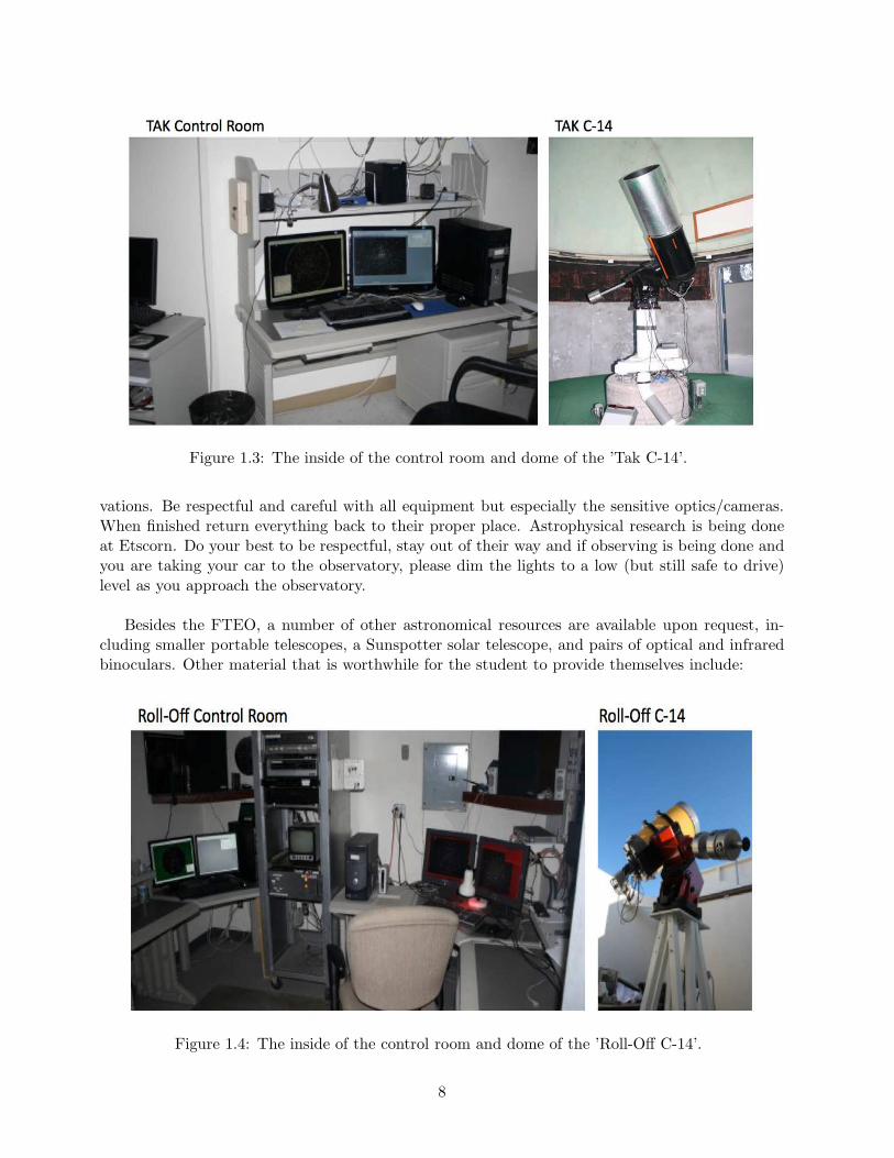
Figure 1.3: The inside of the control room and dome of the ’Tak C-14’.

vations. Be respectful and careful with all equipment but especially the sensitive optics/cameras.When finished return everything back to their proper place. Astrophysical research is being doneat Etscorn. Do your best to be respectful, stay out of their way and if observing is being done andyou are taking your car to the observatory, please dim the lights to a low (but still safe to drive)level as you approach the observatory.

Besides the FTEO, a number of other astronomical resources are available upon request, in-cluding smaller portable telescopes, a Sunspotter solar telescope, and pairs of optical and infraredbinoculars. Other material that is worthwhile for the student to provide themselves include:

Figure 1.4: The inside of the control room and dome of the ’Roll-Off C-14’.

8

1. Stars and Planets (4th edition - or any ed. with up-to-date 2015/2-15 tables) — Jay M.Pasachoff [Or any equivalent text]

2. A flash light with a red covering (e.g. red cellophane)

3. a compass (your cellphone may have this already)

4. a protractor (the big hobby ones are best but a standard small one and a ruler will work)

5. a notebook/pens & pencils

6. (Recommended) if you have a smart device installing a planetarium app (there are severalgood, free ones) is worthwhile

9

Chapter 2

Naked Eye Astronomy

10

2.1 Lab I: Naked Eye Constellations [i/o]

Please answer the following questions on separate paper/notebook. In addition to giving the answer,please include a short description of how you obtained your answer. Make sure to list the referencesyou use (particularly for the last questions). For this assignment, working in groups is not permitted.

2.1.1 Constellations

1) Name two constellations that are visible in the evening sky (dusk - midnight) thisweek?

2) What constellation contains the position: Right Asc: 12h34m56s; Dec: -01o23′

45′′

?

3) What constellation is directly south of Sagittarius? (There may be more than one correctanswer.)

4) Name one constellation that borders Andromeda?

5 - 7) The ’Summer Triangle’ is an asterism that is composed of the stars Vega, Deneb,and Altair. In which constellations do each of these three stars reside?

8 - 9) Sirius is the brightest star in the night sky. What constellation is it in? Siriusis often called the ’Dog Star’. Why does this ’make sense’?

10 - 13) Determine the constellation that each of the following objects reside in:Messier 31, Messier 45, NGC 7000, PKS 2000-330.

14) Suppose you are born on February 1st (birth sign: Aquarius), in what constella-tion does the Sun reside on that day? (Hint: trick question.)

15) If you look high in the sky at midnight on your birthday (assume February 1st),name at least one visible constellation.

16) In what constellation does Jupiter reside on November 1st, 2016?

17) From Socorro, can you ever see any part of the constellation, Horologium? (Assumeyou can see to the horizon.)

18 - 20) Write ∼1 page on the constellation of your choice. Include in the discussion:Where is it in the sky? When is it visible from Socorro (if it is)? Does it contain any especiallyinteresting/famous astronomical objects? If so what, if not what is the visual magnitude of thebrightest star in the constellation? What is the history of the constellation? What is a mythologyassociated with the individual/object represented by the constellation (it need not by exclusivelythe ’Greek’ myth).

11

2.1.2 Naked Eye Observing

Reminder: For any ’observation’ you do (naked eye/binoculars/telescope/CCD) please record thedetails of your observation. These include: the weather/sky conditions; rough estimate of thestability of the seeing (twinkling); location of object in the sky; location and nature [city lights?trees blocking part of the view? etc.] of the ground site where you observe from; time/date ofthe observation; integration time/filters/telescope/etc. [if applicable]; and the members of yourobserving ’team’.

21) Using a star chart determine what the constellation Cygnus looks like and whereto look for it in the sky. Go outside on a clear evening and locate the constellationCygnus. Using ’hand measurements’ estimate the size of the constellation in degrees.Does your answer make sense? Hint: Based on the number of constellations that cover thearea of the celestial sphere, what would you guess is the typical constellation size.

22 - 25) Testing your limiting magnitude: Find a location where you can (comfortably)view the constellation Cygnus for a sustained period. Carefully draw the constellationof Cygnus (or a part of it) as you see it in the sky. Draw the bright stars as wellas the faint stars. Focus your attention on the stars that are just barely visible toyou unaided eye. Record their positions, relative to the bright stars (which form a’cross’), carefully so that you may identify them on a star chart afterward. I expectyou to record at least a dozen faint stars in the Cygnus area so that you have goodstatistics. Once you have sketched the faint stars (please include your sketch with theassignment) consult the Field Guide, a star chart or an online database to determinethe visual (V) magnitudes of your faint stars. On your sketch label the name of thestar and its V band magnitude. Determine what is the magnitude of the faintest starsyou identify. (Suggestions: 1) Let you eyes dark adapt for ∼10 minutes before beginning; 2) tryto choose a reasonably dark site to observe from; 3) a red flashlight may be helpful to see the paperto sketch; 4) the more carefully you sketch the position the more likely you will correctly identifythem on a star chart.)

12

2.2 Lab II: Constellations and Stellar Magnitudes [o]

For this assignment, working in small groups is permitted for the observations, however each stu-dent should do their own measurement of the constellation position and brightness. Reminder: Forany ’observation’ you do (naked eye/binoculars/telescope/CCD) please record the details of yourobservation. These include: the weather/sky conditions; rough estimate of the stability of theseeing (twinkling); location of object in the sky; location and nature [city lights? trees blockingpart of the view? etc.] of the ground site where you observe from; time/date of the observation;integration time/filters/telescope/etc. [if applicable]; and the members of your observing ’team’.

2.2.1 Constellations

The purpose of this assignment is to teach you how to find your way around the night sky. This willbe done by asking you to identify several constellations and draw their locations in the sky whenyou observe them. This assignment may be repeated a couple of time throughout the semester.Working in small groups is permitted for the first part but the remaining parts should be doneindividually. All students should have their own sketch of the constellations.

2.2.2 Exercises

1) Find the following constellations in the night sky: Cygnus, Lyra, Aquila, Cassiopeia,Pegasus and Sagittarius. (You may consult a star chart or planetarium app to helpyou recognize and locate the constellation, but once found you must put it away andnot consult it until problems 2 - 3) are fully completed.)

2) Draw a sketch of the constellations (only sketch the main backbone of the constel-lation, but attempt to include at least six stars) listed above in their correct locationsat the time you observe them, on the provided sheet. Be sure to note the exact timeof your observations and careful identify the direction corresponding to North. Youwill use the same map for all constellations. Pay particular attention to the relativeposition in the sky, the angular separations of the stars and the apparent brightnessof the stars. Use the ’hand method’ for estimating angular separations1.

3) For each constellation number the six brightest stars in order of their decreasingbrightness. Pick the brightest star in all six constellations listed and call this star’zeroth’ magnitude. Next adopt ’fifth-magnitude’ for the faintest stars you can de-cern. Estimate the stellar magnitudes of the other stars by extrapolating between 0-ththrough 5-th magnitude. Compare each star to the other stars and to the two limitingcases. Do not use catalog or star chart magnitudes when doing this problem. Thepurpose of this problem is to help you understand how to estimate stellar magnitudebased on stars in the field.

1The hand method is crude but useful tool for estimating angular separations. Holding your hand out at armslength and close one eye. The angular size projected by the width of your pinkie fingernail is ∼ 1o. 2o

∼ the widthof a finger, 10o

∼ the width of your fist, and 25o∼ the width from thumb tip to pinkie tip of a fully spread hand.

Intermediate angles can be built up from combinations of these measures.

13

4) Once you have completed sketching the constellations and estimating magnitudesbased solely on your observations consult a star chart such as Stars & Planets to seehow well you did. What correlation do you notice between the naming convention ofstars in the star chart and their apparent magnitude?

5) Take a piece of standard letter paper and cut out an 8”times8” square. Hold this’window’ at arms length perpendicular to the direction your are looking. Count thenumber of stars you are able to see through this window towards a random loca-tion in the sky. Record the number of stars and the location you are looking onthe chart you drew the constellations. Repeat for at least two other random loca-tions on the sky. Record these on the chart. Average the number of stars you seein the three measurements. Next calculate the solid angle your window projects onthe sky (you will need to measure the distance from your eye to the aperture anduse elementary geometry to calculate this). This will give you a measure of theN = (# of stars visible)/(solid angle of the window). Scale this number to the 4π steradi-ans of the full sky to obtain an estimate of the number of visible stars in the night sky(only half of which are potentially viewable at any given time of the year. Compareyour numbers to the true number (look up online) and discuss differences / uncer-tainties.

6) The constellations that you are being given are from the western European tra-dition which are derived from Greek and Roman cultures. Each culture has its ownstories about the sky. Find a story associated with one of the above star groups froma different culture and describe.

14

Figure 2.1:

15

2.3 Lab III: Celestial Sphere / Coordinates [i/o]

For this assignment, working in small groups is permitted for the observations, however each studentshould do their own measurement of the stellar position. Reminder: For any ’observation’ you do(naked eye/binoculars/telescope/CCD) please record the details of your observation. These include:the weather/sky conditions; rough estimate of the stability of the seeing (twinkling); location of ob-ject in the sky; location and nature [city lights? trees blocking part of the view? etc.] of the groundsite where you observe from; time/date of the observation; integration time/filters/telescope/etc.[if applicable]; and the members of your observing ’team’.

2.3.1 Coordinate Systems

The usefulness of a coordinate system on the surface of a sphere is apparent to anyone trying tonavigate the surface of the Earth. As such it makes sense to generate coordinate systems for the’virtual’ spherical surface of the sky (the celestial sphere). There are any number of ways to ac-complish this but here we focus on two, the altitude-azimuth and equatorial systems.

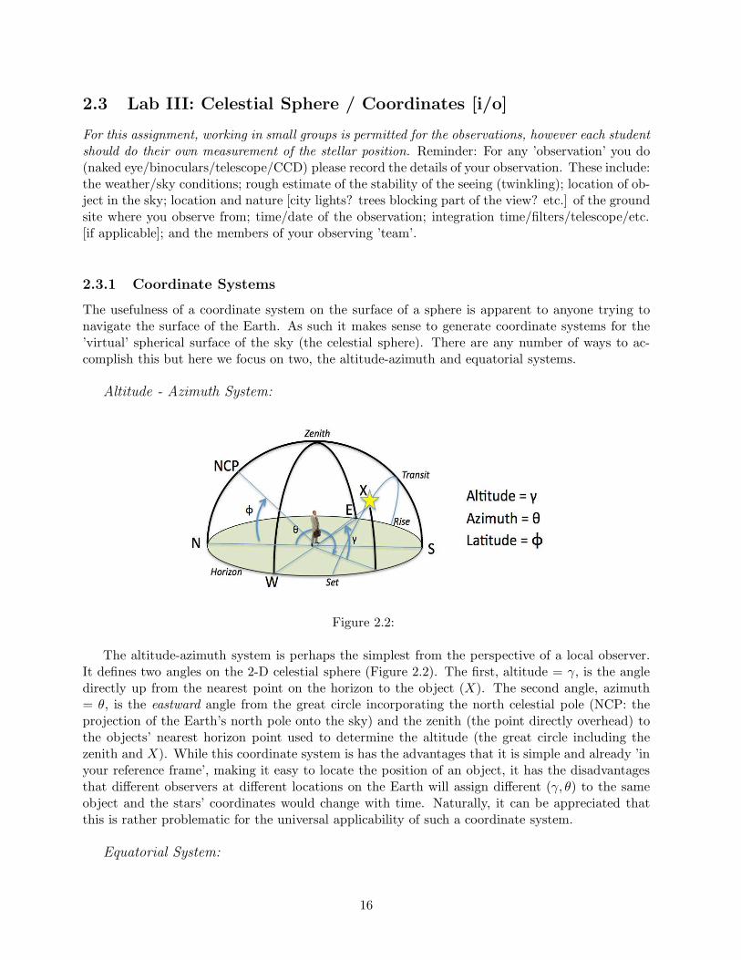
Altitude - Azimuth System:

Figure 2.2:

The altitude-azimuth system is perhaps the simplest from the perspective of a local observer.It defines two angles on the 2-D celestial sphere (Figure 2.2). The first, altitude = γ, is the angledirectly up from the nearest point on the horizon to the object (X). The second angle, azimuth= θ, is the eastward angle from the great circle incorporating the north celestial pole (NCP: theprojection of the Earth’s north pole onto the sky) and the zenith (the point directly overhead) tothe objects’ nearest horizon point used to determine the altitude (the great circle including thezenith and X). While this coordinate system is has the advantages that it is simple and already ’inyour reference frame’, making it easy to locate the position of an object, it has the disadvantagesthat different observers at different locations on the Earth will assign different (γ, θ) to the sameobject and the stars’ coordinates would change with time. Naturally, it can be appreciated thatthis is rather problematic for the universal applicability of such a coordinate system.

Equatorial System:

16

Figure 2.3:

The other commonly used alternative is to select a coordinate system permanently attached tothe celestial sphere. Here we project Earth’s latitude - longitude system upward to the celestialsphere (Figure 2.3). The longitude equivalents (or meridians) are given the name right ascension,α, and are reported in hours:minutes:seconds from 0 hr - 24 hr (for reasons that will become appar-ent momentarily). α are great circles running through the NCP and the SCP, with the particularone running through zenith referred to as your meridian (sometimes just meridian). An objectpassing your meridian is said to be transiting. Also from the geometry of Figure 2.3, the altitudeof the NCP (roughly the star Polaris) is equal to the observer’s latitude, φ, along this meridian.Just as the zero point of the longitude system on Earth is arbitrary (currently the longitude linerunning through Greenwich, England), so to is the zero point of right ascension. We arbitrarilychoose the zero of the right ascension to be the observed location of the Sun on the vernal equinox.[Note: remember that unlike the stars, the Sun appears to move across the celestial sphere. Atthe vernal equinox, roughly noon on March 21st (not counting DST), the Sun is at the locationwhere the ecliptic intersects the celestial equator (Figure 2.4).] When viewed from above the northpole, α increases in the counter-clockwise (eastward) direction. Because of the Earth’s rotation,the celestial sphere appears to rotate east to west in a regular fashion. Hence right ascension ticksby your meridian like a clock, hence the units (Figure 2.4, right).

The clock metaphor is quite good, with the following two caveats, 1) unlike typical dial clocksyou are used to, the hour hand (your meridian) remains fixed and the dial (right ascension on thesky) rotates clockwise (when facing south) past the hand, and 2) the clock dial has 24 hours insteadof 12 hr. From this we can define a couple of time related concepts. The first is hour angle, H,which is the difference between the α(your meridian) and α(object) (- if east of your meridian and+ if west). The second is local sidereal time, LST , (’star time’). LST is defined as:

LST = α + H, (2.1)

and corresponds to either the α(meridian) or the hour angle of the right ascension = 0 line. Know-ing your LST and your latitude uniquely defines the appearance of the night sky. The latitudeequivalents for the sky are given the name declination, δ. They represent the projection of the

17

Figure 2.4:

Earth’s latitude lines onto the celestial sphere. The projection of the Earth’s equator, fittinglyenough called the celestial equator, marks the zero of declination. Declination lines are parallel tothe celestial equator (and hence are not great circles), with + for the northern hemisphere and -for the southern. The apparent path of the Sun across the celestial sphere is called the ecliptic andis inclined 23.o5 from the celestial equator (Figure 2.4). Therefore the position of the Sun on thevernal equinox is (α, δ) = (00:00:00, 0).

Converting Between Systems:

Since alt-az coordinates are often simpler to work with from an observational perspective, itis worthwhile gaining experience converting between the two coordinate systems. By measuring(γ, θ) and knowing φ, we can convert alt-az coordinates to equatorial by use of spherical trigonom-etry. Figure 2.5 illustrates the relevant geometry. From spherical trigonometry, with the followingassumptions: 1) a triangle, with interior angles a, b, c, lying on the surface of a unit sphere, 2) all(angular) sides ABC are great circles, and 3) all sides and angles are expressed in angular units,then we can use the spherical cosine law:

Side B : cos(B) = cos(A)cos(C) + sin(A)sin(C)cos(b)

Side C : cos(C) = cos(A)cos(B) + sin(A)sin(B)cos(c).

Or given that A = 90 − φ, B = 90 − δ, C = 90 − γ, a = parallactic angle, b = 360 − θ, and c = H:

sin(δ) = sin(φ)sin(γ) + cos(φ)cos(γ)cos(θ), (2.2)

and

cos(H ′) =sin(γ) − sin(φ)sin(δ)

cos(φ)cos(δ), (2.3)

where H ′ is the hour angle converted to angular units. Equation 2.2 can be used to obtain thedeclination, δ, once you have measured the altitude and azimuth of the object (γ, θ). Once youhave δ, equation 2.3 can give you H. Next you can get ST , by remembering that ST=00:00:00at noon on March 21st and shifts forward (24/365) hr per day and 1 hr per hr on a given day.[Example: ST (Nov 4th @ 6 pm) = (227/365)×24 hr + 6 hr = 20 hr 56 m — do not forget to ac-count for daylight savings time if applicable.] Equation 2.1 can then be used to find α given H andLST . Using other spherical trigonometric relations relations it is possible to develop the reverse

18

conversions (get γ, θ from α, δ) but we will not focus on it here. (If you care to try to calculate therelations, use eq. 2.3 to solve for γ instead of H, and use the sine rule to get θ in terms of H, δ and γ).

Given this long-winded introduction, the goal of the assignment is to measure the γ, θ of a star ata given (sidereal) time and from that derive the α, δ and compare to catalogs to verify your accuracy.

Figure 2.5:

1) Locate Polaris (the tail star of the Little Dipper). Measure the angle from thenorthern horizon to Polaris. Assume this gives φ, the latitude of Socorro. To do thisyou will need a compass to locate north-south so that you may determine your merid-ian and a protractor (angle measuring device) in order to determine φ. Compare tothe true value (Google Earth is very convenient for this).

2) What is δ for an object at zenith?

3) Locate some object in a sky chart that appears to be on your meridian. Record its(α, δ). Calculate the α of the meridian given the LST . Is α of your object equal to theα you calculated? Discuss any discrepancies.

4) Locate the star α Scorpii (Antares) in the sky. Measure and record its altitude, γand its azimuth θ at a given time. Draw a sketch similar to figure 1, for your star andlabel your measured angles.

5) Calculate the right ascension and declination of Antares from your measurements.Look up the α, δ of Antares and discuss any discrepancies (both measurement andassociated with incorrect/inaccurate assumptions.)

6) Calculate the azimuth of Antares’s rise, assuming α and δ are known quantities

19

(hint: what is γ for an object just rising?). Determine the clock time of its rise (hint:since it is up in the sky your answer should be before the current clock time.)

20

2.4 Lab IV: Earth - Sun - Moon System [i/o]

Please answer the following questions on separate paper/notebook. Make sure to list the refer-ences you use (particularly for the last questions). For this assignment, working in small groupsis permitted for the observations. Reminder: For any ’observation’ you do (naked eye / binoculars/ telescope / CCD) please record the details of your observation. These include: the weather/skyconditions; rough estimate of the stability of the seeing (twinkling); location of object in the sky;location and nature [city lights? trees blocking part of the view? etc.] of the ground site where youobserve from; time/date of the observation; integration time/filters/telescope/etc. [if applicable];and the members of your observing ’team’.

The coupled motions of the Earth and Moon lead to a number of important effects for the Earth-Sun-Moon system. These motions are of fundamental importance for wide range of subjects, includ-ing the appearance of the day/night sky, our place in the solar system, Earth’s seasons/weather,our system of timekeeping, even to humanity’s socio-political structure. In this assignment you willmix theoretical calculations with careful observations of the Sun/Moon/Stars to better understandthe important Earth-Moon motions.

2.4.1 Sidereal vs. Synodic Period

The apparent motions of the Sun and stars are due to the complex motion of the Earth, includingrotation, revolution and precession of the axis. To reasonable approximation orbits are circular.The subtleties come from the coupled nature of the motion. Because of this there are multipledefinitions of key times like day, month and year, depending on the point of view adopted. Takethe day for example. There are two different definitions of the day, 1) the sidereal day — the timeit takes for the Earth to rotate 360o on its axis relative to the distant stars, and 2) the solar day –the time it takes the Sun to go from on your meridian back around to your meridian again. Sincethe Earth revolves while it is rotating, these two times are not the same. We define the hour as1/24th of a solar day, so a Solar day is 24 hr long. For the Earth both rotation and revolutionare counter-clockwise as viewed from above the north pole. Hence the Earth must rotate a littlebit extra to get a given spot on the surface of the Earth pointing back toward the Sun, becausethe angle between the Earth and Sun has changed relative to the stars due to the small amountof revolution within the day (see Figure 2.6). By geometry the extra amount of time required tocover the extra angle is, textra = (1 day/365.2422 day)*24 hr = ≃4 min. Therefore the siderealday is ≃23h56m. Since our clocks are synchronized to 24 hr, if we return look at the sky at thesame exact clock time the next day, the stars will appear to have moved 4 min westward. Orstars in the sky appear to rotate at a sidereal rate of 1o (well technically 360

365.2422

o) westward per so-

lar day. This is in comparison to the apparent rotation rate of stars on a given day of ≃ 15o per hour.

In this assignment you will observe the sky to confirm these motions both for a day and thecorresponding effects for the month.

1) Find a bright star on your meridian. (How do you know if the star is on themeridian?) Record your ground position and exact clock time/date. Now wander offand have a good time. Return to your spot exactly 1 hr later, find the star and measurethe angle off your meridian, including direction and an estimate of your uncertainty,

21

Figure 2.6: Due to the extra counter-clockwise revolution of the Earth around the Sun, the Earthmust rotate an extra 1/365.24 fraction of a circle (4 min) to return the Sun to the meridian.

(this is the Hour Angle: + to West, - to the East). From your measurements estimateby how much do the stars appear to move in a 1 hr period, due to the rotation ofthe Earth? Discuss whether your answer conforms to what you expect given youruncertainties. You will need to be cognizant of the declination of the source in this measurement.

2) Find a bright star on your meridian. It makes sense to use the same one youadopted in problem 1). Record your ground position and exact clock time/date (oruse those from problem 1). Come back to the exact same spot at the same timebetween 2-4 days later (depending on weather for example) and measure the angleoff the your meridian. Repeat the above after waiting between 8 - 12 days and afterapproximately one month. From your measurements estimate by how much do thestars appear to move in a 24 hr period, due to the difference between the siderealand solar day? Discuss whether your answer conforms to what you expect given youruncertainties.

For the Moon the sidereal month is again the time it takes for the Moon to complete one orbitrelative to the distant stars. The Synodic or Lunar month is the time for the Moon to cycle throughits phases (e.g. return to the same Earth-Moon-Sun relative geometry).

3) Following the analogous arguments for the sidereal day vs. solar day, sketch thegeometry of the Earth-Moon-Sun system necessary to calculate the synodic (lunar)month, given that the sidereal month is 27.3217 days. Include at least two (important)positions of the Moon in the diagram (as in Figure 2.6). The Moon also revolves counter-clockwisewhen viewed from above.

4) Using your sketch calculate the length of the synodic (lunar) month. Do you bestto get four significant digit accuracy.

5) Use two lunar eclipses, which to good approximation meets the requirement ofthe Moon having the exact same phase, to determine the Synodic month. (You mayfind lists of lunar eclipses in Stars and Planets. Try selecting lunar eclipses that areroughly a year apart.) Also look up the true Synodic month in a reference. Discuss

22

the accuracy of your measurement and possible reasons for any discrepancies betweenthe three numbers.

6) The Moon is tidally locked to the Earth (the same ’face’ of the Moon alwayspoints toward Earth). What is 1 ’lunar’ (analogous to a ’solar’) day on the Moon (Sundirectly overhead to the next time the Sun is directly overhead)? Explain why.

2.4.2 Moon Phases

Figure 2.7: The geometry of the Earth - Moon - Sun system for determining Moon phases. If youare standing on the Earth’s surface at the location of the tick mark and the corresponding Moonphase is on your meridian, then the clock time is given.

We are all aware that the position of the Sun in the sky is a (reasonably) accurate clock (in factthe first good clock). This clock is not exact (consider the solar analemma), but sets the basis of theday. So how could you tell time at night if you didn’t have a mechanical one? Moon phases resultfrom the relative geometry of the Earth - Sun - Moon system (Figure 2.7). A combination of theposition of the Moon and its phase will tell you where the Sun is in the sky and hence can be usedto tell time. As a simple example consider the Full Moon. The fact the phase of the Moon is fullindicates that the Sun is 180o away from the Moon. So if the Full Moon is on your meridian, then itis local midnight (e.g. the Sun is at the Nadir). This of course does not include humanity’s changingof clock time, for example Daylight Savings Time, and other subtle effects you are to contemplatein problem 9. For the case when the Moon is not at your meridian then you must remember therate at which the Moon (and stars) appear to ’rotate’ across the sky. For example, in our FullMoon case, if the Full Moon was at an hour angle of -2 hr (towards the east) then the Moon is 2 hrfrom reaching meridian, hence the Sun is 2 hr from reaching Nadir. So you clock time must be 10pm.

In this portion of the assignment you will watch the cycle of the phases of the Moon proceedthrough >1 month and determine the time based on the moon phase/position.

7) If you go out (in the northern hemisphere) at 3 am and see a gibbous moon highin the southern sky, is it a Waxing or Waning gibbous? Explain your reasoning.

23

Figure 2.8:

8) Observe the Moon’s phase over a period of more than one lunar month. Youneed not observe every night but you should have at least six measurements dispersedthroughout this period. For each observation make sure to record the time you didthe observation, the position of the Moon in the sky (altitude-azimuth) and the phase(percent illuminated). Be as precise as you can for the Moon phase. Here binocularsmight be helpful in seeing precisely where the terminus of the shadow occurs on theMoon. But this is not required (your answer for the the next part will be more preciseif you are careful). Sketch the phase of each observation on a sheet of paper or in yournotebook.

Figure 2.8 assists you in determining the relative phase/geometry for case when the Moon isnot in an obvious phase like first or third quarter, or full etc. If you carefully locate the shadowterminus on lunar features then you can consult a Moon map to accurately determine the angu-lar extent of the illuminated portion, L, compared to the true angular diameter, Dm. The ratioL/Dm = 1

2(1− cosθ) gives θ, where θ is the angle from the New Moon geometry (noon if the NewMoon is at your meridian).

9) For two of your measurements, use the phase of the Moon together with itsposition on the sky to calculate the clock time (do not forget to account for daylightsavings time if applicable). Compare this to your recorded clock time. Discuss anydiscrepancies between the two.

24

2.5 Lab V: Lights and Light Pollution [o]

For this assignment, working in small groups is permitted for the observations, however each shouldturn in their own list. Reminder: For any ’observation’ you do (naked eye / binoculars / telescope/ CCD) please record the details of your observation. These include: the weather/sky conditions;rough estimate of the stability of the seeing (twinkling); location of object in the sky; location andnature [city lights? trees blocking part of the view? etc.] of the ground site where you observefrom; time/date of the observation; integration time/filters/telescope/etc. [if applicable]; and themembers of your observing ’team’.

2.5.1 Lights

One of the key culprits for decreasing the joy and splendor of the night sky is light pollution.Because so many of us live in cities light pollution is a major concern. However, some things canbe done to minimize light pollution by controlling the type and shielding lights have.

In this assignment we will judge the quality of lights on the NMT campus in terms of lightpollution. The provide ”Night Spectra Quest” contains a small diffraction grating that will allowyou to determine the type of light source you are looking at. The types of lamps that you mightfind around campus are listed on the back of the card. You might want to make a copy of thethat list so you don’t need to keep turning the card over and over. By the time you are donewith this project you should have memorized the spectra of the various lamps. In order to see aspectrum when looking through the grating you need to hold the card horizontal, length parallelto the ground, look through the hole at the light and then look either to the left or the right to seethe spectrum.

Figure 2.9:

You will be given map of the NMT campus with a portion highlighted to select. Your mission,if you accept (and you have no choice), is to count the number of each type of light source either ona pole or attached to a building in your selected territory. You do not need to count light sourcescoming from inside a building. Looking at the spectra on the back of the card you can see that thelights that gives off the least amount of light are the low pressure Mercury and Sodium. Basically

25

they have no continuum light. The other important factor in reducing light pollution is how thelight is projected. Figure 2.9 gives you examples of different quality light projection schemes.

In fact it is the law in New Mexico that all outdoor lights over 75 Watts must be up withina shield so that the lamp cannot be seen when the observer is at eyelevel with the bottom of theshield. This is really hard to comply with for lights on the sides of building. Designers tend tobelieve that putting more light is better than proper shield. But you can see from the image thatthe little person standing next to the light has the best view when the light is directed down andnot into your eyes.

So what I want from each student is a list of the types of lights, how many of eachkind and the quality of the shield. Mark locations on the map for each light source.Label each light source with the following label (a-j)/(1-4). The letters a - i wouldcome from the card. And the letter ”j” would stand for other types of light not onthe card. For the shield parameter, ”1” is the worst and ”4” is the best. For a lightsource on a building that is not pointed down you could use ”5”. I suspect that all ofyou have some kind of cell phone camera, so a few pictures would be nice.

Include a short (∼1/2 page) summary of the lights in your section of campus. Arethey well designed or bad light pollutors? Which lighting types do you personally feeldo the best job of safely illuminating the area? Are areas overlit? Underlit? For thosewho live off campus, you might briefly try the same experiment in your neighborhood.Are the results different from campus? How so?

26

Chapter 3

Telescopic Techniques

27

3.1 Lab VI: Introduction to Telescopes / Optics [i/o]

Please answer the following questions on separate paper/notebook. Make sure to list the refer-ences you use (particularly for the last questions). For this assignment, working in small groups ispermitted. Reminder: For any ’observation’ you do (naked eye/binoculars/telescope/CCD) pleaserecord the details of your observation. These include: the weather/sky conditions; rough estimateof the stability of the seeing (twinkling); location of object in the sky; location and nature [citylights? trees blocking part of the view? etc.] of the ground site where you observe from; time/dateof the observation; integration time/filters/telescope/etc. [if applicable]; and the members of yourobserving ’team’.

3.1.1 Simple Astronomical Refracting Telescope

The simplest of astronomical telescopes are built of two converging lenses, one typically of longfocal length (fob; objective) and the second of short focal length (fep; eyepiece), separated by adistance, fob + fep. Figure 3.1 labels the geometric setup of a simple astronomical refractingtelescope. From figure 3.1 we see that the lens combination acts to angularly magnify (m ≡ α′/α)and invert the image of a object.

Figure 3.1: A simple astronomical refracting telescope. The l is a shorthand notation for a con-verging lens. The simple astronomical telescope is an inverting instrument.

From the leftmost triangle we see that in the small angle approximation α′ ≃ h/siep . From thecentral triangle we further see that α ≃ h/soep ≃ h/(fob +fep). Making use of the basic lensmaker’sequation: 1/fep = 1/siep + 1/soep , it can be demonstrated that m = fob/fep. Namely for a giveneyepiece focal length, fep, a long objective focal length, fob leads to high magnification, while for agiven objective focal length, a short eyepiece focal length leads to high magnification. Furthermore’f/ratio’ (written f/#) can be defined as, f/# ≡ fob/Dob, where Dob is the diameter of the objec-tive lens. The f/# is solely of function of the design of the objective lens. For a given Dob, biggerf/# imply high magnification, while for a given fob, bigger f/# imply smaller light grasp (see below).

28

3.1.2 Schmidt-Cassegrain Telescopes

Many of the telescopes you will use are not simple refracting telescopes, but the above conceptscan be fairly easily adapted to apply. For simple (Newtonian) reflecting telescopes the focal lengthof the objective is just the distance from the mirror to the focus point of the converging (or diverg-ing) rays. Etscorn Observatory has a number of Schmidt-Cassegrain telescopes. The focal pathof Schmidt-Cassegrains are folded and so a bit more complex. Here we just use its reported focallength as fob. However it can be determined from the optics of the mirrors, with fob correspondingto extending the converging rays from the secondary lens back along the line until they reach thediameter of the telescope, Dob.

SCT fob ≃ fmfb/(fm−d), where fm is the focal length of the primarymirror, fb is the distance between the secondary mirror and the focal plane, and d is the distancefrom the secondary mirror to the primary mirror.

Figure 3.2: Schematic of a Schmidt-Cassegrain, with its focal length drawn.

The TA will demonstrate the use of the Schmidt-Cassegrain telescopes at Etscorn,including use of the domes, checking the collimation of the telescopes, focusing thetelescope and pointing the telescope using the TheSky6.0 software.

3.1.3 Field of View

The field of view (FOV) of a telescope depends on its optics, both the objective and the eyepiece.To a crude approximation the FOV of the simplest eyepieces are, FOVep ∼ Dep/fep, where Dep

is the diameter of the eyepiece lens (or more properly any limiting aperture stops inside). How-ever, modern eyepieces have become optically quite complex and so nominally we take the FOVep

(often referred to as ’apparent FOV’) of an eyepiece as a given. They are often written on theeyepiece directly. Low quality eyepieces, like the Hyugens, Ramsden and Kellner types typicallyhave a FOVep ≃ 25 − 45o. Very high quality, wide field eyepieces, such as Erfles and Naglershave FOVep ≃ 65 − > 82o. However the typical common use eyepieces, such as Plossls andOrthoscopics, have intermediate FOVep ≃ 50o. Due to magnification the FOV of the telescopesystem, FOVtel, is much smaller. The telescopic magnification ’zooms in’ on the FOVep by a factorequal to the total magnification. So telescopic FOV (often referred to as ’true FOV’) is given by

29

F OVtel = F OVep/m.

The larger the FOV the larger fraction of diffuse astronomical objects that can be viewed simul-taneously. The angular drift rate of an object on the sky is 15o/hr × cos δ, (δ = declination). Sofor simple telescopes without tracking motors, larger FOVs also mean longer times for the object tobe viewed without readjusting the pointing of the telescope. However, larger FOV naturally implylow magnifications.

3.1.4 Resolving Power

In the (better) wave theory of light, the point source response function (or point spread function;PSF) is the Fourier transform of the aperture function (the shape of the aperture). For circularapertures of size, Dob, the PSF is an ’Airy disk’. From the central peak to the first null of an Airydisk is θ1/2 = 1.22 λ/Dob, so a star viewed in the visible (λ = 5500 A) will exhibit a full widthzero intensity (FWZI) size of 2× θ1/2(”) ≃ 280/Dob(mm). No objects spaced by less then this cantheoretically be separated completely. Small telescopes, with perfect optical systems, well focused,on sturdy mounts, and in very stable atmosphere can reach close to the theoretical limit. But sincethese are difficult conditions to obtain, practical resolving power of an aperture rarely is this good.For larger apertures, the atmosphere limits resolving power to about 1-2

′′

. A typical approximationto estimate the ability to resolve two point sources (up to the atmospheric limit) is to assume oneFWZI PSF separation between the two sources. With this assumption then point sources (stars)that are separated by s ≃ 4θ1/2 = 560/Dob(mm), ought to be resolved by an objective of sizeDob. This roughly corresponds to ’20/20’ vision in daylight.

3.1.5 Maximum & Minimum Useful Magnification / Exit Pupil

The eye’s aperture at night ranges from 5 - 7 mm, so from s ≃ 560/Dob(mm), we obtain the resolv-ing power of the unaided eye to be roughly s ∼ 100

′′

, or about 118 th of the size of the Full Moon.

This practical limit of the eye implies a maximum useful telescope magnification. Any telescopicmagnification that magnifies the maximum theoretical limit of the aperture (≃ 140/Dob(mm))greater than 100

′′

is of no practical use. Doing so would just result in zooming in on the unre-solved blob of light limited by the telescope optics and not lead to seeing any finer detail (andjust make it appear fainter — see the Surface Brightness subsection). Inserting numbers, oneobtains mmax ≃ 0.75 − 1.0 × Dob(mm), or phrased in terms of the eyepiece focal length:fep(min) ≃ f/#(objective). Therefore for small hobby telescopes, the maximum useful magnifica-tion is ∼ 100 - 150×. The larger, stably-mounted telescopes at Etscorn can support roughly twicethis magnification. Note: these numbers are approximate and depending on the observer, site andquality of the telescope, these numbers vary somewhat.

The exit pupil, Dex, is the physical size of the image of the objective as seen through the eye-piece. From Figure 3.3 it can be seen that α = (Dex/2)/fep = (Dob/2)/fob, hence the exit pupilsize is given by Dex = (fep/fob)×Dob or Dex = Dob/m. The higher the magnification for a givenobjective focal length, the smaller the exit pupil. This is why it often takes some effort to get youreye aligned properly to see the image when working at high magnification. The exit pupil also con-trols the minimum useful magnification of a system. If the exit pupil gets bigger than 7 mm, thenthe entire light collected by the telescope is not focused down tight enough to completely enter the

30

Figure 3.3: The geometry for determining exit pupil.

eye. For a completely dark-adapted eye aperture of 7 mm, this implies a mmin = Dob(mm)/7.It is for this reason that most astronomical binoculars tend to be manufactured such that the ratioof the magnification to the objective is ∼7 (such as 7 × 50, 12 × 70, 15 × 80), and ’terrestrial’binoculars have the above ratio of ∼4 (Deye in daylight; such as 8 × 25, 10 × 42).

3.1.6 Light Grasp / Surface Brightness

Light grasp, GL, represents how much more light an objective collects compared to the eye. It issimply given by the ratio of the area of the objective to the area of the eye, and hence is roughlyGL = (Dob(mm)/7)2. Light grasp is the main benefit of large telescopes, not so much magnifica-tion, as seen in the previous section.

When magnifying by m, a scope spreads (roughly) the same amount of light over a surfacearea m2 larger. Hence the surface brightness, SB, of an object is m2 fainter. However a scopealso collects more light, in proportion to GL. So the surface brightness of an object when viewedthrough a telescope is:

SBtel = SBeye ×GL

m2=

(

Dob

Deye

)2

(

fob

fep

)2

(as long as Dex < Deye), where SBeye is the surface brightness the object would have with theunaided eye. The maximum SBtel corresponds to the case when the magnification is minimum,m = mmin, so SBmax = SBeye. The best surface brightness a telescope can provide is that of theunaided eye! A telescope just makes that same surface brightness be observed over a larger area.(Note: this does not account for ’integration time’. Surface brightness sensitivity can be improvedby ’integrating’ longer than the eye does or by using more efficient photon detectors like CCDs —more later.) We define SBeye as 100%. Thus:

SBtel(%) = 100% × GL

m2=

(

fep

Deye

)2

(f/#)2= 2% × fep(mm)

(f/#)2.

High magnification makes objects large but dim, while low magnification keeps objects bright butcompact.

31

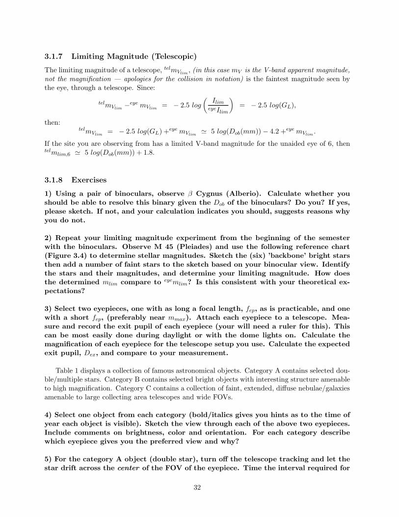
3.1.7 Limiting Magnitude (Telescopic)

The limiting magnitude of a telescope, telmVlim, (in this case mV is the V-band apparent magnitude,

not the magnification — apologies for the collision in notation) is the faintest magnitude seen bythe eye, through a telescope. Since:

telmVlim−eye mVlim

= − 2.5 log

(

IlimeyeIlim

)

= − 2.5 log(GL),

then:telmVlim

= − 2.5 log(GL) +eye mVlim≃ 5 log(Dob(mm)) − 4.2 +eye mVlim

.

If the site you are observing from has a limited V-band magnitude for the unaided eye of 6, thentelmlim,6 ≃ 5 log(Dob(mm)) + 1.8.

3.1.8 Exercises

1) Using a pair of binoculars, observe β Cygnus (Alberio). Calculate whether youshould be able to resolve this binary given the Dob of the binoculars? Do you? If yes,please sketch. If not, and your calculation indicates you should, suggests reasons whyyou do not.

2) Repeat your limiting magnitude experiment from the beginning of the semesterwith the binoculars. Observe M 45 (Pleiades) and use the following reference chart(Figure 3.4) to determine stellar magnitudes. Sketch the (six) ’backbone’ bright starsthen add a number of faint stars to the sketch based on your binocular view. Identifythe stars and their magnitudes, and determine your limiting magnitude. How doesthe determined mlim compare to eyemlim? Is this consistent with your theoretical ex-pectations?

3) Select two eyepieces, one with as long a focal length, fep, as is practicable, and onewith a short fep, (preferably near mmax). Attach each eyepiece to a telescope. Mea-sure and record the exit pupil of each eyepiece (your will need a ruler for this). Thiscan be most easily done during daylight or with the dome lights on. Calculate themagnification of each eyepiece for the telescope setup you use. Calculate the expectedexit pupil, Dex, and compare to your measurement.

Table 1 displays a collection of famous astronomical objects. Category A contains selected dou-ble/multiple stars. Category B contains selected bright objects with interesting structure amenableto high magnification. Category C contains a collection of faint, extended, diffuse nebulae/galaxiesamenable to large collecting area telescopes and wide FOVs.

4) Select one object from each category (bold/italics gives you hints as to the time ofyear each object is visible). Sketch the view through each of the above two eyepieces.Include comments on brightness, color and orientation. For each category describewhich eyepiece gives you the preferred view and why?

5) For the category A object (double star), turn off the telescope tracking and let thestar drift across the center of the FOV of the eyepiece. Time the interval required for

32

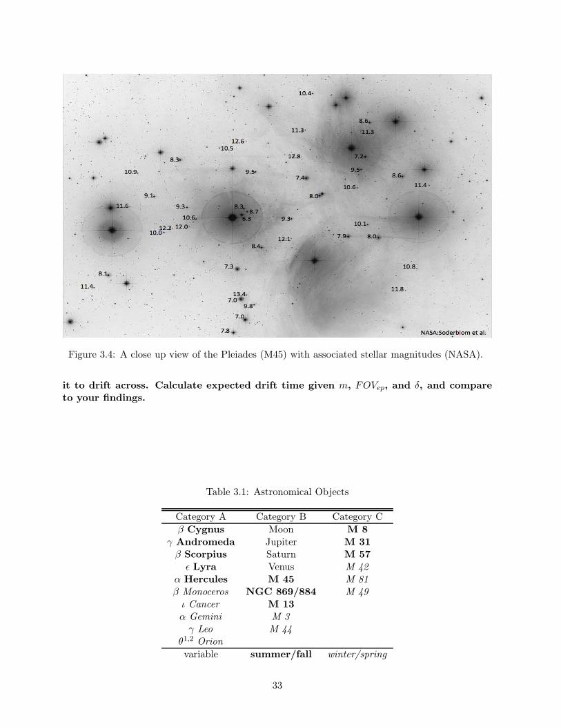
Figure 3.4: A close up view of the Pleiades (M45) with associated stellar magnitudes (NASA).

it to drift across. Calculate expected drift time given m, FOVep, and δ, and compareto your findings.

Table 3.1: Astronomical Objects

Category A Category B Category C

β Cygnus Moon M 8γ Andromeda Jupiter M 31

β Scorpius Saturn M 57ǫ Lyra Venus M 42

α Hercules M 45 M 81β Monoceros NGC 869/884 M 49

ι Cancer M 13α Gemini M 3

γ Leo M 44θ1,2 Orion

variable summer/fall winter/spring

33

3.2 Lab VII: Introduction to CCD Observing [o]


3.2.1 Introduction to CCDs

CCDs (charge coupled devices) are devices that convert individual photons of light into electriccurrent. CCDs have revolutionized astronomy, allowing even small ’amateur astronomy’ telescopesto generate images of the quality of >1-meter class telescopes + film. As a feature of the 1970ssemi-conductor revolution, CCDs have the great advantage of being nearly linear, highly efficientphoton detectors. The quantum efficiency, Qe, of CCDs are typically ∼75%, compared to the ∼1% offered by film.

CCDs convert photons to e− by a process similar to the photoelectric effect (though the e− donot leave the material). When a photon strikes an atom in a semi-conductor an e− can be knockedout and promoted into a weakly bonded (free to flow) ’conduction band’. These e− can then betrapped by a electric potential and steered to a counting device (Figure 3.5). Pixels are read out ina ’bucket brigade’ (’pass the bucket along’) fashion, with rows of e− containing pixels being passedacross the array. The end pixels passing their e− to a serial register, which are then shifted downthe serial register one-by-one to a read out amplifier (Figure 3.6). By keeping careful track of thetiming one can reconstruct the location on the array that is currently being read out. When theCCD is being read out, integrations are not occurring.

Figure 3.5: Left) The energy band structure of a semi-conductor. Right) A schematic of a simplifiedCCD pixel (Wikipedia).

34

3.2.2 CCD Properties

There are a number of important properties associated with CCDs. We review some of these here(Table 1 and 2 list several of the important characteristics of the CCD you will use at Etscorn):

• Pixels: Each element in the array is a pixel. Sizes of modern arrays are in the millionsof pixels. The physical size of the pixel is important for setting the resolution of the array.The Etscorn Tak dome’s CCD has a native pixel size of 6.8µm, but can be binned 2 × 2 or3 × 3 (to give lower pixel resolution, but higher sensitivity). When coupled with the opticsof the telescope it is possible to determine the ’plate scale’, ps, of a CCD/telescope setup.The ps is the (angular dist.)/(physical dist.) on the focal plane. The plate scale for a simpleastronomical telescope is:

ps(rad/mm) = 1/fobj(mm) − or − ps(”/mm) = 206265/fobj (mm). (3.1)

Or finding the ps in terms of pixel size:

ps(”/pxl) = [206265/fobj(mm)][s(mm/pxl)], (3.2)

where s is the physical pixel size. For the Etscorn CCD in medium res. mode (2× 2 binning;Table 2), the pixel size is, s = 13.4 × 10−3 mm. The fobj(native) of the C-14 is 3911 mm,however the telescope has been equipped with a (roughly) ×2 focal reducer, so the actual fobj

is about 1955 mm, so ps(”/pxl) ≃ 1.4.

• Quantum Efficiency: The fraction of photons falling on the detectors that are actuallyregistered and result in production of an electron. Obviously the higher the number thebetter. Typical Qe are ∼ 75 % for good CCDs and tend to be somewhat better at the redend of the spectrum than the blue. The Qe of the human eye is between 5 - 10 % dependingon whether you are using the rods or cones.

• Errors/Uncertainties: CCDs have sources of noise/uncertainties:

– Bias: The e− in a pixel when no light is shining on it. It can be calibrated out by takinga zero second ’exposure’.

– Dark Current, Dc: Thermal energy can cause e− to be excited into the conduction band.This thermally generated signal is called dark current. Dark current is a strong functionof temperature, so cooling CCDs greatly reduce dark current. In good cooled CCDs darkcurrent is often very low. For the SBIG ST-10 CCD at Etscorn Dc = 0.5e−/sec/pxl.Dark current is calibrated out by taking an exposure of exactly the same integrationtime as the target, but with the shutter closed, and then subtracting it off the targetobservation.

– Read Noise, RN : Read noise is the amplifier noise associated with reading out eachpixel. It is not a Poisson process and hence its S/N ratio does not reduce with thenumber of counts, CNT .

– Flat Fielding: The Qe of every single pixel is not the same. Different pixels have differentsensitivities. To normalize out this effect, we need a uniform, white source to image totell us the relative response of each pixel. Taking the corresponding flat, white image iscalled flat fielding.

35

– Saturation (’Full Well Capacity’): There is a maximum number of e− that a pixel canhold. If the pixel reaches this level then a new incoming photon will not be able toproduce a measurable e−. Integrating longer will not result in any more e− detected,and so saturation sets constraints on the length of time you can integrate for a givenbrightness source. For the Etscorn CCD, the full well capacity (the number of e− a givenpixel can hold) is 77,000.

– Gain, g: An image count (CNT) need not be equal to one e−. In fact it is in generalnot. The conversion between e− and CNT (or ADU) in an image is given by the gain.For the Etscorn CCD, g = 1.3e−/CNT . Since the CCD has a gain of 1.3 e−/CNT, thatmeans that the CCD saturates at 60,000 CNTS. Going above this count number in animage means you have saturated and hence lost linear (or any) relation between numberof photons detected and counts registered. Adjust integration time, filters, or aperturessuch that you do not go above this number if you are doing quantitative work.

Figure 3.6: Left) Schematic of the read out of a CCD chip. Right) A picture of the SBIG ST-10CCD that is on the Etscorn Observatory C-14 telescope.

Table 1

Parameter Value

CCD Kodak KAF-3200ME

# of Pixels 2184×1472Pixel Size 6.8×6.8 µmFull Well Capacity ∼77,000 e−

Dark Current 0.5 e−/pxl/secExposure 0.12 - 3600 secA/D gain 1.3e−/CNTRead Noise 8.8e−/pxl RMS4500A Qe 62 %

6500A Qe 82 %Cooling 1 stage, H2O-assisted

thermoelectric fan

T regulation 0.1 oC

Table 2

Mode Full Frame Half Frame Quarter Frame

High Res. 2184×1472 1092×736 584×370(unbinned) 6.8µm 6.8µm 6.8µmMed. Res. 1092×736 546×368 275×186(2×2) 13.6µm 13.6µm 13.6µmLow Res. 728×490 364×245 184×124(3×3) 20.4µm 20.4µm 20.4µm

36

3.2.3 CCD Observing

Calibration: Figure 3.7 shows the basic calibration strategy for CCD imaging. One obtains sev-eral flat field frames (aim for high S/N but not near saturation - say 10,000 CNT; and then averageto make a master ’flat’), (optionally) several bias frames (tint=0 sec, then average to get a master’bias’), then one integrates on the target for the needed time, tint, and on the ’dark’ for the sametime. The ’dark’ is subtracted from the ’target’, and the ’bias’ from the ’flat’, respectively. Thenthese two outcome files are divided to give the final image. The TA will give instructions on howto do this with the available software.

Sensitivities: We also need to have some idea as to the amount of integration time you willneed to detect an object. In this assignment, you will essentially determine this by trial and error,but in the long run it will be useful to be able to estimate this ahead of time. Given here is anapproximate ’CCD equation’ for determining the sensitivity required. The signal-to-noise per pixel,S/N |pxl, of an object of brightness mV can be given as:

S/N |pxl =PtarQetint

(PtarQetint + PskyQetint + Dctint + RN2)1/2, (3.3)

where Ptar (Psky) is the rate of photon arrival per pixel per sec for the target (sky). Ptar is oftenlooked up in tables for a given telescope but we crudely calculate it below. Since the collecting ofphotons (or e−) is a random process, the standard deviation increases as the

√CNT , so that S/N

increases roughly as the√

CNT (in the ’photon noise’ limit). When the signal CNT gets low, thenthe Dc and RN terms become significant and alter the S/N behavior.

Figure 3.7: The basic CCD calibration strategy.

37

A useful rule of thumb to remember is that a V-band = 0th magnitude star generates a photonrate, P ′, of 1000 γ s−1 cm−2 A−1. The C-14 at Etscorn has an aperture of roughly 103 cm2, and ifwe crudely estimate that the width of the V band filter is 1000A, then we obtain a photon rate ofP (V = 0) ∼ 109 γ s−1. However, this flux of photons (or e− in the pixels) are not focused into onepixel. Normally you will try to have several pixels across a resolution element (either the resolutionof the telescope optics or the atmospheric seeing). So crudely estimating a star is spread over 10pixels (assumed uniformly illuminated) then Ptar(V = 0) ∼ 108 e− s−1 pxl−1 (note: the image isnormally spread over closer to 100 pxl and not uniformly illuminated, so this is a bit of an optimisticestimate). One can find the Ptar(V ) for any V band magnitude by: Ptar(V ) = Ptar(0) ∗ 10−0.4V .

The sky is not, in general, completely dark. Roughly (at a decent site) the sky has a V bandsurface brightness of ∼ 20mag/arcsec2. So this flux and the noise associated with it contributesto the noise budget. We can estimate the photon (or e−) rate associated with the sky, by a similaranalysis as above, except that because the sky is extended, we have the count rate per pxl withoutthe further correction needed for the star. For the CCD in medium res., full frame mode, the ps is∼1.4”/pxl, so msky(mag/pxl) = msky(mag/”2) − 2.5log(ps2) ≃ 19.6. Therefore if we assume thesky brightness is ∼19 mag/pxl, then Psky ≃ (109e−s−1pxl−1) ∗ 10−0.4∗19 ≃ 25e−s−1pxl−1. Dc, Qe

and RN for the Etscorn CCD are given in Table 1. Using these numbers we obtain that in a tint

= 1 sec integration on a V=0 mag star, we have a S/N ≃ 9000 (does not include issues related tosaturation). Likewise for the same tint, V= 5, 10 and 15 mag correspond to S/N per pixel of 900,90, and 6, respectively.

3.2.4 Differential Photometry

Often one wants to determine the magnitude of an object in the sky. To determine this by doing ab-solute photometry (measuring relative to a reference calibrator like an A0 star) can be rather trickyand we do not discuss the subtleties here. However, if you have multiple sources in a single image,say one being considered a known reference magnitude and the other being the target of interest,then one can effectively do differential photometry. This is where you measure the CNT on a sourceof known magnitude and then use that to set the ’zero-point’ to convert between CNT and mag.Since m1−m2 = −2.5log(F1/F2), then it can be seen that mtar = mref +2.5log(Fref )−2.5log(Ftar).By measuring Fref and Ftar from the image, and knowing the magnitude of the reference, thenyou can determine the magnitude of the target star. The differential nature of this photometry isimportant, because you are looking through the same patch of atmosphere, therefore eliminatingmost of the atmospheric related corruptions.

3.2.5 Assignment

In this assignment you will become familiar with the techniques needed to execute CCD imagingwith the 14” at Etscorn. The TA will lead you through the steps to operate the dome, telescope andsoftware on site. But here I list the basic observations / analysis that you are expected to do forthis assignment.

1) Turn on the dome, telescope and software systems. Establish a working direc-tory on the computer. Focus the telescope. Choose the V band filter from the filterwheel. Obtain several ’flat field’ frames by observing the inside of the dome. Do notforget to record the instrumental set up parameters for each file taken. The header

38

of the .FIT (Flexible Image Transport System) files do include some of this useful information.Working with the CCD in 2x2 binned medium resolution mode is fine.

2) Locate the RR Lyrae star AV Peg (see Figure 3.8 for information on its posi-tion, magnitude and ephemeris). Take target frame-dark frame pairs at a number ofroughly log spaced tint. Say something like 0.3s, 1s, 3s, 10s, 30s etc. or whatever turnsout to be relevant for this source. Calibrate each frame and then plot the source CNTon AV Peg vs. tint. (The calibration can be done directly in the software and themeasurements of the CNT [or flux] can be done in a number of packages, ’fv’ beinga fairly simple one.) Find a ’blank spot’ in the image and measure the RMS of theCNT in the same size region used for the source. Plot RMS CNT vs. tint.

3) The figure caption of Figure 3.8 gives information about the stars in the AV Pegfield. Two stars, of magnitude 9.34 (labeled 93) and 9.53 (95), are near AV Peg. Theirdistances from AV Peg are given. By measuring the number of pixels between eitherstar and AV Peg in the image and comparing to the given separation you will obtaina plate scale in ”/pxl. Compare this to that expected theoretically for the system.

4) Choose just the best tint for AV Peg (high S/N but not with the CNT nearsaturation values) and repeat integrations with that tint on AV Peg once every 1/2hour (or so) for at least three hours. Note: the members of the group [or groups] can splitup the 3 hours and have one group do the early observations and another the later observations ifwished.

5) Determine the V band magnitude of AV Peg for each measurement from dif-ferential photometry on each of the ’93’ and ’95’ reference stars, and average. Plotthe V band magnitude vs. time. Do you see it vary? At the level it should have?(http://www.aavso.org/vsp may be useful here.)

6) RR Lyrae stars have roughly constant absolute magnitudes of MV ≃ 0.75. Thismakes then useful (and famous) as ’standard candles’ for determining distances toastronomical objects [e.g. globular clusters and galaxies]. Using your determined Vband apparent magnitude, derive the distance to AV Peg assuming its absolute Vband magnitude is the standard 0.75.

7) Select any two deep sky objects (see for example the Messier and Caldwell Cat-alogs in Stars and Planets) that do not completely fill the FOV of the CCD. Make andpresent a V band calibrated image of each. Once you get comfortable, these may be donequickly between your 1/2 hour waits for AV Peg.

39

Figure 3.8: A finder chart for the AV Peg area. The coordinates, V band magnitude range, and variability periodare shown. (At least) two reference stars useful for differential photometry are labeled. The star labeled 93 has aV magnitude of 9.34 and is separated by 295” from AV Peg. The star labeled 95 has a V magnitude of 9.53 and isseparated by 403” from AV Peg.

40

3.2.6 Appendix A: CCD observing at Etscorn Observatory

Here is a very short summary of an example observing session at the Etscorn Observatory 14” SCT.The TA will give a much more detailed introduction at the telescope. (Subject to change.)

Start Up:

— Turn the computer on (and login) in the control room (CR)— Open up the SkyX application on the computer (telescope and CCD control)— Open telescope control, focus control, camera control and find windows

>display>[telescope control, camera, focuser, find]— Remove the white sheet and the lens cap from the telescope— Turn the telescope, the mount, and the CCD camera on in the dome— Create subfolders < flats >, < raw > and < final > in working directory— Connect SkyX to the telescope

>telescope>startup>connect telescope- find home? = yes

Flat Fielding:

— Connect SkyX to the camera— In SkyX camera control set the camera to cool down:

>camera>temp setup — select ∆T to cool CCD— While cooling, turn on white light at base of telescope mount, position dome so telescope points to the wall— In SkyX set the camera exposures (odd number):

>camera> — Select filter>camera> — Select exposure time>camera> — Toggle subframe=on (full field)- Take exposures till you are happy with the # of counts in the flat>camera> — Toggle autosave=on, set path to < flats > folder>camera>setup>autosave; [when happy with the setup]- Take odd # of exposures to median

— Open up the CCDSoft application on the computer- (In CCDSoft do not ’connect’ to the camera.)

— In CCDSoft make a master flat:>image>combine>combine folder of imagesselect path < flats >select all flat .FIT files>median>combine>combine [highlight image window] >file>save as> < flats > folder— Save combined master flat as a .FIT file.

Focusing:

— Turn on focus paddle— Focus the telescope with the hand paddle/mask (the software should hold focus as the temperature changes).

- select star to focus on:>find>slew

— Open and align dome slit to new position (the dome slit ’overshoots’ so go slowly when almost fully open)— Click off all dome lights

>camera> — Select exposure time>camera>Take Photo — take exposure, find star in image

— In dome, put focus mask on telescope— Check focus

>camera>Take Photo — take exposure, note the starburst pattern on all stars>focus> — change focus in steps, take exposure- take exposure>focus> — Adjust focus setting till you observe the middle spike centered between the other two spikes- repeat exposure till happy with focus>focus>add datapoint>focus>activate

— In dome, remove focus mask from telescope

Observing:

— You are now ready to take science images.>find> enter name; or select lists>slew to slew- Select integration time, filter, turn autosave=on (if you wish to save image); autodark=on

— In SkyX set image path to < raw >, adopting a rememberable nomenclature— [Alternatively you can leave autosave off and save manually. But if so be careful to not forget to save all needed files!]

41

— take images>camera> — Select exposure time>camera>Take Photo — take exposure

— Save dark corrected files as .FIT files in < raw > (if not autosaved).

Data Reduction:

— Reopen the CCDSoft application on the computer— Apply the master flat field to images:

- In CCDSoft apply flat:>image>reduce>flat fieldchoose master flat from < flats > folder and image to flat field from < raw > folder>okay- save corrected image as .FIT in < final > folder- Repeat for all science images

Shut Down:

— In SkyX ’home’ the telescope and disconnect:

>telescope>startup>find home to slew to home

>telescope>shutdown>disconnect to disconnect telescope once homed

>camera>disconnect to disconnect camera

— Close SkyX

— Close CCDSoft

— Power off the mount, telescope and CCD camera

— Put lens cap on the telescope and white sheet completely over the telescope

— Close up the dome slit (the dome slit ’overshoots’ so go slowly when nearly closed)

— Turn off any dome lights and lock dome

— Save you data somewhere that you can take with you

— Shut off computer and monitor .

42

3.3 Lab VIII: Introduction to CCD Color Imaging [o]


3.3.1 Introduction to CCD Color Imaging

Color information is one of the best tools we have as astronomers to understand the physics occur-ring in an object (whether it be ’broadband’ or ’spectral line’). Different radiation mechanisms emitat different wavelengths and so by comparing different wavelengths we can constrain the relativeimportance of the different emission mechanisms (or other properties such as temperature).

In a previous lab you became familiar with basic CCD / telescope operation and simple reduc-tion / analysis. The goal of this lab is to extend this so that you can obtain color images (andbegin to contemplate the science associated with the color). Color imaging is done by making anumber of single wavelength (filter) images and then combining them in post-processing. Typicalastronomical filters available in the optical include U, B, V, R, and I. Figure 3.9 shows the trans-mission fraction as a function of wavelength for the filters at Etscorn along with the Qe of the CCD.Nominally the B (Blue) filter peaks around 4450A and has a width of ∼1000A, while V (’visual’or green) peaks around 5500A and has a width of ∼900A, R (red) peaks around 6600A and hasa width of ∼1400A, and I (’infrared’) peaks around 8000A and has a width of ∼1500A. Another’filter’ is the L or luminance ”filter”, which is clear — that is it is equivalent to no filter or just theblack line in Figure 3.9. The CCD does not have the same sensitivity in each filter. The relativesensitivity of the CCD in a filter is the integral of the transmission weighted by the CCD response.Notice that the combination of the CCD response and the bandwidth of the filter makes CCD mostsensitive in R. Because the sensitivities are unequal you will need different integration times (or totake more images of the same integration time) to achieve equivalent sensitivities in each filter. [Ofcourse the color of the object also influences the brightness in each band, but that is the sciencewe are after.]

The basic strategy behind color imaging is to proceed just as you did for a single filter observa-tion, but then repeat those steps individually for each filter (typically at least three filters are usedso that you can build an RGB color image. Make sure to obtain a separate flat field frame for eachfilter. You will then use the CCDsoft software to combine the reduced images in each band into acolor map:

Make Color Image (In CCDSoft):

— Open four combined images in < final > folder— Align the images:

— click the star/tack icon on top of main window

43

Figure 3.9: The filter response (transmission fraction) vs. λ in nm (10A).

— select the same star in each image— click >Image>Align>Align Centroid

— Combine the images to make a color image:— click >Image>color>color combine— Correctly associate the B filter with the blue channel, V with the green, R with red and

L with luminance— click ’reset’ and ’show preview’

— Adjust the histograms for each color until the image in the preview window makes a goodcolor image:

— >Histogram Editor>adjust sliders— Your goal is to adjust the histograms such that the background is black and the majority

of the stars are white (or close to it)— When you are happy with the preview click >combine

— Save your beautiful color image somewhere, again with a understandable naming conventione.g. M57 rgb. Note: The resultant image with be a bitmap and not a .FIT file.

The Instructor/TA will give you a more detailed explanation at the telescope.

In this class you will want to image in the B, V, R and L bands. The first three will give youthe red - green - blue RGB components and the last, through no filter, gives you the overall whitelight response.

3.3.2 Assignment

1) Pick a relatively bright deep sky object (the Messier or Caldwell catalogs are agood place to start) of interest to you (preferably one that has significant color differ-entiation to it). Observe it at Etscorn to obtain the best color image you can. Selectionof several candidate objects that you expect to be interesting (and bright enough to be doable),should be done ahead of time. Come prepared!

44

2) Summarize your observing strategy and details of the success/problems associ-ated with getting a good color image.

3) Once you have obtained a nice color image of the object, describe the imagein careful detail (please send me both a print out of the image and a copy of theelectronic image file). It should take you at least a paragraph to describe suitablyquantitatively. Note features such as overall colors and shapes, as well as fine detaillike wisps, dust lanes, voids, etc... [I don’t want just ’It’s round and blue” or the like.]

4) Find an online color image of the object and compare to yours [cite its refer-ence]. Do they agree? How do the observational/instrumental differences betweenthe Etscorn telescope you use and the one used to take the comparison image impactany differences you see?

5) Write at least a one page typed report on the astrophysics of your chosen ob-ject. Include the four component images (BVRL), the color image (in color) andthe online reference image (also in color) Make sure that a major component of thewrite up focuses on the reasons for the colors you observe. This should be writtenin a fairly formal ’report style’, including citation of all referenced literature. Here Idemand that you include at least one peer-reviewed research journal article in yourdiscussion. (Do not give me just encyclopedia/textbook/wikipedia descriptions.) Important ref-erence webpages that will help you include the NASA Astrophysics Data System [NASA-ADS:http://adsabs.harvard.edu/abstract service.html] to find the literature articles, the SIMBAD As-tronomical Database [SIMBAD: http://simbad.u-strasbg.fr/simbad/] for detailed information onGalactic sources, and the NASA Extragalactic Database (NED: http://ned.ipac.caltech.edu/) forextragalactic objects.

45

3.4 Lab IX: Introduction to Spectroscopy [o]

Please answer the following questions on separate paper/notebook. Make sure to list the references you use (particu-

larly for the last question). For this assignment, working in groups is permitted. Reminder: For any ’observation’ you

do (Spectroscope/CCD) please record the details of your observation. These include: the weather/sky conditions;

rough estimate of the stability of the seeing (twinkling); location of object in the sky; location and nature [city lights?

trees blocking part of the view? etc.] of the ground site where you observe from; time/date of each observation;

integration time/filters/telescope/etc. [if applicable]; and the members of your observing ’team’.

3.4.1 Introduction

The light from astronomical objects are extremely rich, carrying vital information on the object’scomposition, temperature, densities, internal structure, and dynamics to us. Spectra from theseobjects are a complex mix of continuum emission, absorption lines and emission lines. The nature ofthe emission mechanism depends on the part of the spectrum one observes. In the optical, emittedlight tends to be associated with hot ionized gas and stars, which exhibit temperatures of thousandsof degrees K. The continuum emission of most bright objects are (very roughly) thermal blackbodyemission associated with hot (∼3000 - 30,000 K) objects. Absorption and emission lines are relatedto quantum electronic transitions between atoms (both neutral and ionized) and molecules as theseare transitions have characteristic transition energies of ∼few eV (1 eV = 11,600 K in temperatureunits).

3.4.2 Stellar Spectroscopy

With a spectroscope, we can split the incoming optical light into its constituent wavelengths andbegin to investigate the information carried in the spectrum. Here we focus on stars and ionizedgas nebulae (HII regions), as they are the brightest objects in optical spectra. Most of the emissionfrom stars are continuum in nature. The emission originates from the hot, opaque interiors of thestar. As it leaves the star it passes through a more diffuse, transparent stellar atmosphere, whichimprints a series of absorption lines atop the continuum. Because of hydrostatic equilibrium, themore massive the star, the higher the pressure and hence the hotter and bluer the continuum. Thestrength of the spectral lines seen in the atmosphere depend both on the excitation and temperatureof the atmosphere. We know that the atmosphere of stars are mainly H (and some He), but theselines are not always the strongest (in absorption). At very hot temperatures (> 30, 000 K) H isprimarily ionized, making neutral H abundances small and Balmer H lines weak. As temperaturesdrop too low then little H is excited out of the ground state and the Balmer (n=2) lower state isunpopulated. The optimal temperature of Balmer absorption lines occur at about 10,000 K. Atcool temperatures of a few thousand degrees, the small excitation gaps associated with metals andeven molecules come to dominate. Figure 3.10 gives a very schematic view of the expected stellarspectral properties as a function of temperature.

The stellar temperature axis is often characterized by spectral classification rather than tem-perature. The standard spectral classification goes as O, B, A, F, G, K, M, (and for brown dwarfsL, T). The earlier in the alphabet the more prominent the H Balmer series, so A stars have themost prominent Balmer lines and hence have temperatures around 10,000 K. The spectral classifi-cations are further subdivided by arabic numerals from 0 - 9, with 0 being hottest and 9 coolest.

46

Finally a luminosity classification, marked by Roman numerals is included. ”V” means dwarf ormain sequence stars, ”III” means giant stars and ”I” are supergiants. The spectral classification ofthe Sun (a 1 solar mass main sequence star) is G2V. Spectral lines in the atmosphere are pressurebroadened and so linewidths are related to the stellar atmospheric pressure. Giants and supergiantsare very large stars with puffy, low density / pressure atmospheres and hence narrower spectrallines. However, given our spectroscope’s resolution, this can be difficult to distinguish.

3.4.3 Ionized Nebular Spectroscopy

Diffuse ionized clouds of gas (HII regions — the ’II’ = singly ionized, while ’III’ = doubly ionized,’IV’ = triply ionized, etc.) are different from stars in a number of respects. These difference resultin qualitatively different spectra. Firstly, the HII regions are generally hot, low density and freefrom (optical) continuum emission. Therefore, by Kirchoff’s laws, we expect the HII regions to havea pure emission line spectrum. Secondly, for typical solar metallicity environments, it happens thatheating and cooling rates conspire to keep HII region at a roughly constant electron temperatureof about 10,000 K. The temperature of the nebula is set by balancing heating rates associatedwith energetic photons from the massive stars’ radiation and cooling rates from recombination lineemission. The hotter the star the higher the heating rate. But the higher the heating rate, themore excited and ionized the nebula becomes and hence the more species / transitions availableto recombine and emit photons that carry energy away from the cloud. In solar metallicity gas,abundances of trace species like C, N, O, S, Ne and their partially ionized forms, are enough tocool the gas down to ∼10,000 K even for much hotter stars. Because of these two points, we expectthat the observed spectra to reflect gas abundances for a plasma of about 10,000 K. Lines such asthe Balmer lines of H, plus low ionization states of C, N, O and S (e.g. CIII, NII, OI-OIII, SIIetc.), and HeI are common.

0

0.2

0.4

0.6

0.8

1

2000 3000 4000 5000 6000 7000 8000 9000 10000

Nor

mai

lized

inte

nsity

Wavelength (Angstroms)

24000K12000K

6000K3000K

Visible Range

Ionized H, He

Neutral H, He

Ionized/Neutral metals

Molecules

Figure 3.10: Normalized blackbody curves for four temperatures shown for wavelengths’ somewhatlarger than the visible range (marked). Typical sources of emission/absorption lines at varyingtemperatures are also marked.

47

3.4.4 The Spectroscope

Figure 3.11: The interior of the SBIG Spectroscope. (Image: SBIG)

In this assignment you will use the Etscorn SBIG - SGS spectroscope + SBIG ST-7 CCD camerato image spectra of a number of the brightest available astronomical objects. The SGS spectro-scope/CCD system contains two CCDs. One is a small square chip, known as the autoguider. ThisCCD gives a normal image of the sky in the direction of the slit. It is this camera that you willuse to place and keep your object of interest centered on the slit. The slit, aligned vertically, cannormally be identified as a dark stripe across the object, when properly centered. An LED canbe turned on inside the spectroscope to illuminate the slit, if you are having difficulties locatingit. (Don’t forget to turn it off before making your science exposures.) The second chip is usedto obtain the object spectrum. It is a rectangular chip of width 765 pixels. The spectrum shouldappear roughly horizontal on this CCD. The more horizontal the better in terms of wavelengthcalibration.

Also provided is a mercury (Hg) pen light for wavelength calibration. (Two important noteswith this light source. 1) Minimize your exposure to the light source as much as possible because itemits a fair amount of UV radiation that can ’burn’ the skin and eyes with prolonged exposure. 2)Do not slew the telescope while the pen light is plugged in. The cable is short and a slew can pullit apart.) Plugging in the Hg pen light will illuminate it and project a Hg spectrum on the CCD(use a short exposure so as to not saturate the chip). The wavelength axis (the horizontal axis ofthe chip) can then be calibrated.

The CCD is controlled by CCDSoft and the telescope by Sky6.0 as before, while the calibra-tion/spectral analysis is done by the computer program, Spectra also available on the same desktop.The calibration procedure is described briefly in Appendix A. The spectroscopy is quite flexible,though we will not use all the modes because they can be tedious to set up. Modes available

48

include two slits, a broad 72µm width and a narrow 18µm width. The broad width slit gives upspectral resolution for increased sensitivity. The narrow slit gives higher spectral resolution butis best suited for bright (naked eye) objects. This assignment will exclusively use the narrow slit.There are two diffraction gratings inside the spectroscopy. One (the low resolution grating) has150 rules/mm and gives a dispersion of 4.27 A/pxl, (for the ST-7 9µm pixels). The spectral resolu-tion is approximately twice the dispersion. The bandwidth of this grating is ∼3300A. The secondgrating has 600 rules/mm and therefore has four times the dispersion/spectral resolution (1.07Adispersion), but 1/4 the bandwidth (it can cover only about 750A at once). A micrometer on thebottom of the spectroscopy can be used to change the central frequency of the spectrum projectedonto the CCD. For this assignment we will use the low resolution grating exclusively. It is currentlyset to accept a wavelength range of about 3600 - 6800 A. This should be acceptable and thereforeadjusting the micrometer is likely not needed.

3.4.5 Spectroscopy Assignment

In this assignment you will become acquainted with the spectroscopy and the spectra of brightstars / nebulae. We will not make use of all the features of the spectroscope, but will use enoughto see its power.

1) Obtain broad band (∼3600 - 7000A) spectra in low resolution mode for a rangeof bright stars of different spectral classifications. I recommend the following stars: γOrion (Bellatrix) — B2III, β Orion (Rigel) — B8I, α Canis Major (Sirius) — A1V,α Canis Minor (Procyon) — F5V, α Auriga (Capella) — G6III, β Gemini (Pollux)— K0III, α Taurus (Aldebaran) — K5III, and α Orion (Betelgeuse) — M2I. Displaythese spectral along a spectral classification sequence so that you can see how thespectrum changes with class.

2) Identify the main spectral features you see in each of the above stars’ spectrum.(You need not identify all of them but do identify the most obvious features). Table1 includes an (incomplete) list of the more important and likely to be observed lines.Describe which features are found in which spectral classification. Do they follow whatis alluded to in the ’Stellar Spectroscopy’ section and Figure 3.10?

3) Comment on the meaning of the shape of the underlying continuum emission ineach spectral class. Does your observed continuum profiles match those shown in Fig-ure 3.10 for the appropriate temperature/spectral class (blackbodies)? If not explainwhy not.

4) The luminosity class of the brightest apparent magnitude red stars you observetend to be giants (III) or supergiants (I). Explain, in terms of ”observation bias”, whythis might be.

5) Estimate the strength of the 6563A Balmer Hα line versus spectral classificationand plot. Normally optical (absorption) spectral line strengths are reported as ’Equiv-alent Widths’ (EW). EW has units of wavelength and is the width of a rectangle havingthe height of the continuum at the line wavelength and the area of the line. That is:

49

Table 1 — Selected Spectral Lines (Incomplete)Line λ Line λ Line λ

OII 3726 HI11 3771 HI10 3798HI9 3825 NeIII 3869 HI8 / HeI 3889CaII [K] 3934 NeIII 3967 CaII [H] 3968HIǫ 3970 NII 3995 HeI 4026MnII 4030 FeI 4045 CIII 4068SrII 4077 HIδ 4101 HeI 4144CaI 4226 Fe/Ca/CH [G] ∼4300 HIγ 4340OIII 4363 HeI 4388 HeII 4541CaI 4454 HeI 4471 MgII 4481HeI 4541 CIII 4647 HeII 4686HeI 4713 HIβ 4861 HeI 4922FeI 4958 OIII 4959 OIII 5007FeI / MgII [b] 5167-5183 MgH band 5210 FeII 5217OI 5577 NeII/NII 5754 HeI 5876Na [D] 5890-6 TiI 6260 OI 6300CrI 6330 FeI 6400 CaI 6440FeI /CaI 6494 NeII 6548 NII 6549HIα 6563 NeII/NII 6583 HeI 6678SII 6717 SII 6731 CaII 8500CaII 8544 CaII 8664TiO band edge: 4750, 4800, 4950, 5450, 5550, ∼5870, ∼6180, 6560, 7050, 7575VO band: 5230, 5270, 5470, 7800-8000, 8400-8600CaH band: 6385, 6900, 6950 O2[terr.]: 6870, 7600 H2O[terr.]: 7150

EW =∫

(1 − Iλ/Icont)dλ, where Iλ is the intensity of the line profile and Icont is the (ex-trapolated) continuum intensity at the wavelength of the line. However, since we havenot calibrated the intensity axis, for this part of the assignment you may simply plot(1−Iλo

/Iconto) vs. spectral class, where Iλois the count value at the deepest point on the

line and Iconto is the extrapolated count value of the continuum at the same wavelength.

6) Take a spectrum of Jupiter or Venus in the same spectral setup. Carefully de-scribe its spectrum. Does it look like a stellar spectrum? If so what spectral class?What modifications from this class do you observe? Why does Jupiter’s/Venus’ spec-trum look this way?

7) Take a spectrum of M 42 (the great Orion Nebula). Do your best to get bothsome of the Trapezium stars (θ1 Orion A-D) and the nebular emission (easy to get)on the slit simultaneously. Identify the brightest spectral features from both the starsand the nebula. Describe the spectrum of this object. Are there emission / absorption/ continuum lines from the stars? From the nebula? (That is does the type of spectralfeature change with vertical position along the slit?) What spectral class would givefor the trapezium stars based on your work in problems 1 - 4? Does this make sensefrom the perspective of them being the ionization source of the Orion Nebula? Arethe HII region lines the same as the stellar lines?

50

3.4.6 Appendix A

You will be led through the basic observing strategy at Etscorn Observatory by the instructor/TAs, but a rough outline is included here:

1. Initiate the usual set up for using the C-14

2. Slew to a bright object.

3. In CCDSoft image the object with the ’autoguider’. Exposures should be very short (∼0.1 for these brightobjects).

4. Using fine motion control, move the object to sit on the slit.

5. Save the autoguider image as an .SBIG file.

6. Plug in the Hg pen light and take a short exposure with the ’imager’. Check to see that you see the characteristicspectrum of Hg. Bright lines include: 4046, 4358, 5461A and a pair at 5770/5791 A.

7. Make a subimage of your calibration image that is ≤20 pixels in the vertical direction.

8. Save this calibration lamp image as an .SBIG file.

9. Unplug the Hg pen light.

10. Open up the Spectra program.

11. Click the ’Load Cal’ spectrum, and input the Hg .SBIG file.

12. Select one of the Hg lines near the red end of the spectrum (the left), e.g. either one of the 5770/5791 pair orthe 5461. Center it between the green vertical lines in the display. Identify its wavelength and select it fromthe ’Identify Spectral Line (Angstroms)’ menu. Select ’Mark line 1’. Using the slide bar on the display, moveto a Hg line on the blue side of the spectrum (e.g. the 4358A), center it, select it from the ’Identify SpectralLine (Angstroms)’ menu, and click ’Mark Line 2’. At which point Spectra will calculate the dispersion (thenumber should come out near 474A/mm) and calibrate the wavelength axis.

13. In CCDSoft take ’imager’ observations of your object. You will need to test different integration times.

14. Make a subimage of your object image that is ≤20 pixels in the vertical direction.

15. Save this object image as an .SBIG file. And as a .FITS file if you wish to load it into other data packageslike fv or ds9 at a later time.

16. Click the ’Load Spectrum’ button, and input the object .SBIG file. The spectrum should be calibrated. Perusethe spectrum with the slidebar in the display. Verify that you can identify spectral features. I recommend

starting with Sirius because it is very bright and has an obvious spectral pattern. If your calibration with theHg is not great then you can further ’self cal’ if the object has the bright Balmer series. You can select twoBalmer lines and repeat the ’Mark Line’ step to calibrate again on the ’science spectrum’.

17. When happy with the spectrum, click ’Write text file’ and the program will save your calibrated object spectrumto a .txt file, on which you can perform subsequent analysis.

18. Slew to a new object, Goto #13 and repeat. Spectra should remember your calibration. If the slit does notproduce a perfectly horizontal spectrum then the wavelength calibration will be somewhat dependent of theposition of the object (vertically) along the slit. To optimize calibration accuracy, try to put the stars in thesame vertical position on the slit.

51

3.5 Lab X: Narrowband Imaging of Galaxies [i/o]

Please answer the following questions on separate paper/notebook. Make sure to list the references you use (particu-

larly for the last question). For this assignment, working in groups is permitted. Reminder: For any ’observation’ you

do (Spectroscope/CCD) please record the details of your observation. These include: the weather/sky conditions;

rough estimate of the stability of the seeing (twinkling); location of object in the sky; location and nature [city lights?

trees blocking part of the view? etc.] of the ground site where you observe from; time/date of each observation;

integration time/filters/telescope/etc. [if applicable]; and the members of your observing ’team’.

3.5.1 Introduction

We have seen that the spectra of different objects are different. When observing extended objectssuch as nebulae and galaxies it is often tedious to try and slide a slit across the whole object todetermine spectral make up. Narrow band imaging permits a rapid characterization of the dis-tribution of an individual spectral line. Then the overall spectrum can be built up by observingthrough a number of narrow band filters.

In this lab you will use the narrow band filters available at the roll-off dome telescope at EtscornObservatory to image the ionized gas in galaxies of different types. The available filters, in additionto the broadband clear filter, are the [SII] (6720A), Hα (6563 A), [OIII] (5007 A) and Hβ (4861A). The Hα and Hβ lines are the Balmer recombination lines of hydrogen and thus trace ionizedhydrogen gas that is in the process of recombining, so called HII regions. The ratio of the Hα to Hβline generally has a constant ratio depending on the radiative transfer in the HII region. Differencesin the Hα/Hβ, tend to be due to extinction, since extinction is wavelength dependent. [OIII] and[SII] are higher excitation lines and therefore requires more energetic photons to excite. Often the[OIII]/Hβ and [SII]/Hα ratios (relatively free of extinction) are used to gauge the level of excitationin an ionized region. A particularly common use of these ratios is for identifying/characterizingAGN (accretion onto a black hole) emission (high ratios) versus normal stellar ionization (low ra-tios).

3.5.2 Assignment

In this assignment, you will use narrow band filters to image a couple of galaxies and look for changesin their line emission properties. Given the sensitivity expected in these observation, detailed lineratios are not the focus. Qualitative comparisons between the stellar (clear filter) and ionizedemission will be the focus. You are to observe the galaxy, M82 (a starburst dwarf), and chooseone from the following list (M 51 (spiral), M81 (spiral), M101 (spiral), NGC 4449 (giant irregular)).

1) Obtain narrow band images in each of the four narrow bands (Hα, Hβ, [OIII],[SII]) for the two galaxies of choice. Follow the procedure used to obtain color images(the color CCD lab writeup is posted on the class webpage) up through the alignmentstage, except with each narrow filter replacing each color image. (It is not necessaryto create an RGB ’color’ image from the narrow bands.) Don’t forget to take flats foreach filter. The Hα and [SII] are in the red while Hβ and [OIII] are in the blue, sothe number of images taken and combined should roughly follow a B:R = 5:2 pattern.Make sure to save the four final combined-aligned narrow band filter images as .fits

52

files for later analysis. Also obtain a clear filter image of each galaxy.

2) Compare the different filter images to the clear image. Do you see differences?Mark or explain where the narrow band filters are relatively brighter. These cor-respond to ionized gas regions. How do they relate to position in the galaxy? Itis potentially likely that for the spiral galaxies you will not see extensive [OIII] and[SII] emission (aside from the continue you see in the clear filter). Is this true? If socompare the [SII] to Hα and the [OIII] to Hβ images. If there is no extra emission inthe [SII] and [OIII] images aside from the continuum, the can serve as ’off’ spectra tocompare to Hα and Hβ ’on’ positions. One easy way to compare images is to use theds9>frames option to blink aligned .fit images. If there is additional emission in theO and S lines, describe how it differs from Hα. Does the nucleus of the spiral galaxiesstand out in emission lines?

53

Chapter 4

The Solar System

54

4.1 Lab XI: Introduction to the Sun and its Cycle [i/o]


4.1.1 Introduction

The Sun is the nearest star and hence provides us a close up look at the nature of a stellar pho-tosphere (visible light surface). The surface of the Sun is a boiling caldron of gas that is laced bymagnetic fields and blemished by dark patches known as sunspots. These sunspots are regions ofenhanced magnetic field strength that are carried across the apparent surface of the Sun by differ-ential rotation. Since the Sun is the prime source of energy for the Earth, the changing propertiesof the solar surface have an important impact on life on Earth.

In this assignment we will investigate a number of surface properties by ’observing’ (both by youand by others) the Sun over a period of time. Observing the Sun without proper protectioncan lead to dire consequences — like blindness. Do not observe the Sun in any wayother than directly instructed (either through an appropriate filter or by projectingthe sunlight onto a viewing screen).

4.1.2 The Solar Sunspot Cycle

Sunspots, while having a degree of randomness, exhibit clear evolutionary trends that yield im-portant information regarding the properties of the Sun. The first important thing to note is thatsunspots follow a cycle. The number of sunspots rise and fall in cyclic pattern with a ∼11.2 yearcycle (well 22.4 year cycle [more below]). Figure 4.1 shows the sunspot number versus time for thelast ∼75 years, along with predictions for the next ∼25 years. Right now we are on the downwardhalf of solar cycle # 24. The sunspot number, N , is defined as:

N = k(10 × g + t) (4.1)

where k is a constant that is observer dependent and established by ’calibration’ (assume k = 2 [toaccount for the back side of the Sun here]), g is the number of sunspot groups, and t is the totalnumber of individual spots discernible. The distribution and number of sunspots are determined bythe behavior of the Sun’s magnetic field. Figure 4.2 shows the distribution of sunspots with solarlatitude versus time. The diagram is referred as a ’butterfly’ diagram because of the distinctivebutterfly wing pattern of the sunspots. It is noticed that as a new solar cycle begins the sunspotsare preferentially seen towards the high latitudes (∼ ±30o) of the Sun. As the cycle progresses thesunspots appear closer and closer to the solar equator. This behavior stems from the wrapping upof the magnetic field in the differentially rotating solar disk.

55

The Sun rotates on its axis (tilted by ∼ 7o) just like the Earth. However, unlike the Earth, thefact that the Sun is not a rigid object means that the pole and equator of the Sun do not rotateat the same rate. To good approximation, a sunspot’s positions on the surface of the Sun is fixed,and rotates east to west with the Sun’s rotation rate, maintaining its given latitude. This alsomakes sunspots a useful probe of the rotation rate of the Sun. Since we are rotating around theSun as we watch it rotate, there is a distinction between the Solar rotation period determined froma stationary distant platform (e.g., stars; ’sidereal’ period) and that observed by calculating theperiod it takes a sunspot to appear to complete one revolution (synodic period).

In this assignment you will observe the Sun once with the Sunspotter solar telescope. TheSunspotter is a specially designed simple refracting telescope that projects a 56× magnified imageof the Sun onto a platform, where you can lay a piece of paper and sketch the Sun, without doingdamage to your eyes. Instructions for its use is written on the side of the device.

Figure 4.1: The sunspot number versus time for the last ∼75 years, along with predictions for thenext ∼25 years. Image from NASA; David Hathaway.

Figure 4.2: The sunspot ’butterfly’ diagram. Image courtesy Mt. Wilson Solar Observatory.

56

1) Explain physically way sunspots appear dark relative to the rest of the Solarphotosphere.

2) Using the Sunspotter, sketch the image of the Sun carefully. Note the sunspotpositions and any other features you see. Compare your sketch to that taken the sameday (weather permitting) by the Mt. Wilson Solar observatory daily sketches foundat http://obs.astro.ucla.edu/cur drw.html. How does your sketch compare?

The Mt. Wilson Solar Observatory (MWSO) has been sketching the distribution and magneticproperties of the Sun (semi-)continuously since 1917! The sketches are wonderful solar resourcesand for the remaining quantitative work, we will make use of this database. The sketches are foundat http://obs.astro.ucla.edu/cur drw.html (”Previous Drawing Archive (via FTP)” link near thebottom of the page). Figure 4.3 illustrates an example of one of the sketches (June 25th, 2000).The plots include the time (UT), date, observing conditions, the sunspots visible, their solar coor-dinates (degrees latitude and longitude — 0o longitude point being the point on the Sun directlyabove Earth), and when available the magnetic field strength and polarity. Each sunspot is labeledby R or V to indicate the direction of the B-field (R = North or ’+’ and V = South or ’−’), and anumber which gives the B-field strength in units of 100 Gauss.

Figure 4.3: A sample Mt. Wilson Solar Observatory sketch of the Sun. Seehttp://obs.astro.ucla.edu/cur drw.html

3) Making use of the MWSO sketches, determine the synodic rotation period of theSun. To do this you will need to pick a sunspot in one of the sketches and then trackits motion across the surface of the Sun. Recording the solar latitude, longitude anddate/time at two times as widely spaced as feasible is the best way to get accuracy.Calculate the rotation period for (at least) two sunspots, one with a solar latitude

57

< 5o, and one with a solar latitude > 35o. You are free (encouraged) to pick any timein the past 75 years of sketches (as long as they include the necessary information).Hint: You might wish to consult Figure 4.1 to determine when the Sun has a lot of sunspots, andFigure 4.2 to determine when you might expect sunspots at the appropriate latitudes.

4) Compare your determined synodic period to the ’official’ values. Discuss anydiscrepancies. Compare the determined period from the < 5o data with the > 35o. Arethey the same?

5) Select a MWSO sketch (it can be one of the same ones as used in problem 3)and calculate the sunspot number using eq. 4.1). Compare it the expected numberdisplayed in Figure 4.1 for that date.

6) Select three MWSO sketches from three consecutive solar maxima. For eachsketch inspect the polarity (direction) behavior of the sunspots in both the northernand southern solar hemispheres. Do you notice any regularities when compared tothe rotation direction of the Sun/sunspots? If so what is it? How does the northernhemisphere behavior compare to the southern hemisphere? How does one 11 yearcycle compare to the next. Use this to give a reason why 22 years is a better indicatorof a complete solar cycle.

7) Qualitatively explain/sketch, in terms of the deforming of the magnetic fieldlines due to differential rotation, why you see the sunspot polarity behavior that youdo.

58

4.2 Lab XII Lunar Mountains [i/o]

Please answer the following questions on separate paper/notebook. Make sure to list the refer-ences you use (particularly for the last questions). For this assignment, working in small groups ispermitted for the lunar eclipse observations only. Reminder: For any ’observation’ you do (nakedeye/binoculars/telescope/CCD) please record the details of your observation. These include: theweather/sky conditions; rough estimate of the stability of the seeing (twinkling); location of objectin the sky; location and nature [city lights? trees blocking part of the view? etc.] of the groundsite where you observe from; time/date of the observation; integration time/filters/telescope/etc.[if applicable]; and the members of your observing ’team’.

4.2.1 Forthcoming

59

4.3 Lab XIII: Kepler’s Law and the Mass of Jupiter [i/o]

Please answer the following questions on separate paper/notebook. Make sure to list the referencesyou use (particularly for the last question). For this assignment, working in groups is permit-ted. Reminder: For any ’observation’ you do (CCD) please record the details of your observation.These include: the weather/sky conditions; rough estimate of the stability of the seeing (twin-kling); location of object in the sky; location and nature [city lights? trees blocking part of theview? etc.] of the ground site where you observe from; time/date of each observation; integrationtime/filters/telescope/etc. [if applicable]; and the members of your observing ’team’.

4.3.1 Introduction

In this assignment you will tackle, in earnest, deriving experimental physics results from a series ofastronomical observations.

The four brightest moons of Jupiter, discovered by Galileo with the ’invention’ of his telescope,are in order of increasing distance from the planet, Io, Europa, Ganymede and Callisto (I Eat GreenCheese). These moons hold a privileged place in astrophysics. Galileo demonstrated that theseobject orbit Jupiter and not the Earth. The fact that these objects orbited Jupiter like a mini-solarsystem helped undermine the pre-Copernican belief that the Earth was the center of the Cosmos.

Figure 4.4: Example of what the image of Jupiter’s moons might look like through a telescope. I= Io, E = Europa, G = Ganymede and C = Callisto.

With Newton’s explanation of Kepler’s law for orbiting bodies, we now know that for circularorbits (which the orbits of the Galilean moons can be considered at the level of this class) withthe central object’s mass much greater than the orbiting bodies, then gravity supplies the neededcentripedal force:

mmv2m

rm=

GMJmm

r2, (4.2)

where mm and MJ are the mass one of the moons and Jupiter, respectively, vm is the orbitalvelocity of the moon and r is the distance from Jupiter’s center to the moon. The orbital velocityis:

vm =2πr

P, (4.3)

where P is the orbital period of the moon. Hence:

P 2 =

[

4π2

GMJ

]

r3. (4.4)

So by determining the period, P , and the radius, r, of the moon’s orbit we may measure themass of Jupiter, MJ . This is the primary goal of this lab assignment. You will set up and under-take an observing strategy that lets you measure P and r. You are allowed three ’knowns’,

60

i) the distance to the Jupiter/moons system, dJ = 6.53 × 1011 m, ii) the angular sizeof Jupiter’s disk, θJ = 44

′′

and iii) you may use webpages (see below) to locate whichmoon is Io at the beginning of your observations, [but you may not use the webpagesto determine orbits of the moons.] (Note: the first two values change with time since bothJupiter and the Earth are revolving around the Sun at different rates. The values I give correspondapproximately to the first week in Feb 2015. If you want more precise values for a given day thatyou observe, consult a planetarium program.)

Such observations sound, in principle, simple to do. Simply observe the Jupiter / moons systemrepeated and watch the ’merry-go-round’ of motion take place, timing P and measuring off theposition (Figure 4.4). However there are a few subtleties, that you as a budding observationalastronomer must consider:

• You need to convert angular separation to a physical scale.

• You will need the maximum possible spatial resolution to get precision measurements, at thesame time not losing field-of-view, so that you can keep as many of the moons in view aspossible.

• Jupiter is very bright and can easily saturate the CCD.

• Orbits are such that they take more than one night to cover an appreciable fraction of anorbit.

So in this assignment you will get experience handling such setup/technical issues to arrive ataccurate results. I discuss hints of each of the subtleties, in turn, below:

• Physical scale: You will need to be able to measure the position of the moon accurately. Theobvious reference given the knowns you are provided is the disk of Jupiter, itself. Because youhave the distance to the system and the angular size of the disk, you will be able to determinethe physical distance covered by one pixel at Jupiter’s distance. From that you can measureseparations in numbers of pixels and convert.

• High resolution: Since you will reference based on Jupiter’s disk, you need as many pixelsacross the disk of Jupiter as possible. Use the CCD is full resolution mode instead of themedium resolution mode we have been using. This will make the CCD pixels be half the size(1/4 the area) of the pixels in your previous images. However read out the full array, so thatyou still maintain the same field of view because the moons extend several arcminutes awayfrom the disk. [This will make your files 4× bigger in size. Make sure you have space forthe files.] Also work hard to get the focus of the telescope the best possible, since a blurrydisk will compromise your measurements. If temperatures change significantly throughoutthe night you might need to focus regularly.

• Brightness: Switching to full resolution mode should decrease the rate at which you saturatethe detector (you have made your ’light bucket’ 1/4 the size), but Jupiter is so bright that itlikely will saturate the CCD even at the shortest possible exposure time, tint. Select the filterwith the narrowest bandwidth (Blue) and tint at its minimum value. This should give you asmall enough count rate such that you can accurately measure the size of Jupiter’s disk, andstill detect the moons. (You will need to play with the image contrast to see the moons.)

61

• You will need to track the positions of the moons for a whole night (and perhaps back-to-back nights) to get a good fraction of a cycle (enough to determine what r and P are). UseIo to do the analysis as its orbit is the shortest, but you can try the other moons sincethey should be in the frame also. The following webpages/applets allow you to plot theconfiguration of the moons at a given time. This will help you identify which moon is Io.[http://www.shallowsky.com/jupiter/ -or- http://www.12dstring.me.uk/jovianmoons.htm]. Irecommend that you take measurements across the entire night and possibly back-to-backnights. So that this doesn’t become to oppressive, I recommend the following observing schedul-ing: the class splits into two groups, each with 3-4 students. On each night one of the groupsobserve. During that night each student observes for about 3 hours and then is relieved byanother group member. Upon both groups completing their observations, all images are sharedamongst everyone in the class so that each student has access to a 9-18 hours of tracking,while only being at the telescope observing for a total of ∼3 hours. [Note: Like ’real astro-nomical observing’ you will be at the telescope for a while but will only need to take a ∼0.1simage once every 15mins or so. So you will have plenty of free time on your hands. Bringsomething to fill the downtime.]

4.3.2 Recommended Methodology

You will need to measure r and P so that you can determine, MJ . There are several possiblemethodologies to do this. I list some variations on the basic theme below (assuming to you will useIo as the moon of choice). I recommend that the class gets together when scheduling and adoptsone methodology for everyone, since you will share data.

1) Image the location of the moon (relative to Jupiter’s disk) on ∼15 min intervals for ∼1/4of a cycle starting at the time when the moon transits/is occulted by Jupiter till it reaches itsmaximum separation. This will directly give r (the maximum separation) and P (say 4× the timeit took to go 1/4 cycle).

2) Measure the time it takes the moon to transit (cross) Jupiter’s disk, ∆t. Combining ∆t andDJ will allow you to calculate vm (remember the Eratosthenes Lab). Then observe at sparser timeintervals to determine the maximum separation of the moon (r) (or have the other group do thiscomponent). Coupling vm with r will give you P (see eq. 4.3).

3) Observe in regularly spaced time increments for as long a feasible. Then plot the separationvs. time. The plot should exhibit a sinusoidally varying pattern. If you observe long enough to beable to fit a sinusoid to the data and predict the maximum separation (and when it occurs) thenyou will have obtained r and P . This method works best if you observe the moon on either side ofits maximum separation.

You can determine when transits and occultations occur by consulting the following webpage:http://www.skyandtelescope.com/observing/a-jupiter-almanac/then select ’Phenomena of Jupiter’s Moons in 2015’ partway down the webpage.

***Important***: Given the nature of the CCD / mount setup, the position on the CCD chipflips 180o when the position of the object crosses the meridian. So if you track Jupiter’s moons ondifferent sides of the meridian throughout an observing run you will need to account for this flip isthe data analysis.

62

4.3.3 Assignment

1) Given dJ and θJ , determine the diameter of Jupiter’s disk, DJ , in meters.

2) Observe Jupiter and its moons repeatedly and regularly over an extended timeperiod. For each observation accurately record the time. After collecting data from ev-eryone, (individually) measure the separation of the moon from the center of Jupiter’sdisk for each observation together with the time. Plot or tabulate the separation (pix-els or physical separation — see problem 1]) vs time.

3) Using some version of the above methodologies, determine, r and P for Io. If youwish to attempt to determine the r and P for another moon in addition to Io then I will give youextra credit.

4) Determine MJ from your r and P . Compare this to the known value of MJ

(cite the source you use to get this information). Please do not look up the mass ofJupiter, or a given moon’s orbital period, before completing the schedule observations.Discuss, quantitatively, any errors between your determination and the correct value.Specifically focus on what piece of the calculation / observation was the cause limitingthe precision of your determination. Again for extra credit: If you happened to havedetermined P and r for a second moon, then determine MJ from that moon andcompare to your original determination. Do they agree? Should they?

63

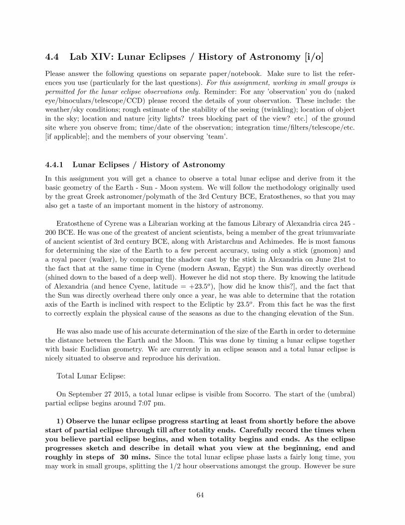
4.4 Lab XIV: Lunar Eclipses / History of Astronomy [i/o]

Please answer the following questions on separate paper/notebook. Make sure to list the refer-ences you use (particularly for the last questions). For this assignment, working in small groups ispermitted for the lunar eclipse observations only. Reminder: For any ’observation’ you do (nakedeye/binoculars/telescope/CCD) please record the details of your observation. These include: theweather/sky conditions; rough estimate of the stability of the seeing (twinkling); location of objectin the sky; location and nature [city lights? trees blocking part of the view? etc.] of the groundsite where you observe from; time/date of the observation; integration time/filters/telescope/etc.[if applicable]; and the members of your observing ’team’.

4.4.1 Lunar Eclipses / History of Astronomy

In this assignment you will get a chance to observe a total lunar eclipse and derive from it thebasic geometry of the Earth - Sun - Moon system. We will follow the methodology originally usedby the great Greek astronomer/polymath of the 3rd Century BCE, Eratosthenes, so that you mayalso get a taste of an important moment in the history of astronomy.

Eratosthene of Cyrene was a Librarian working at the famous Library of Alexandria circa 245 -200 BCE. He was one of the greatest of ancient scientists, being a member of the great triumvariateof ancient scientist of 3rd century BCE, along with Aristarchus and Achimedes. He is most famousfor determining the size of the Earth to a few percent accuracy, using only a stick (gnomon) anda royal pacer (walker), by comparing the shadow cast by the stick in Alexandria on June 21st tothe fact that at the same time in Cyene (modern Aswan, Egypt) the Sun was directly overhead(shined down to the based of a deep well). However he did not stop there. By knowing the latitudeof Alexandria (and hence Cyene, latitude = +23.5o), [how did he know this?], and the fact thatthe Sun was directly overhead there only once a year, he was able to determine that the rotationaxis of the Earth is inclined with respect to the Ecliptic by 23.5o. From this fact he was the firstto correctly explain the physical cause of the seasons as due to the changing elevation of the Sun.

He was also made use of his accurate determination of the size of the Earth in order to determinethe distance between the Earth and the Moon. This was done by timing a lunar eclipse togetherwith basic Euclidian geometry. We are currently in an eclipse season and a total lunar eclipse isnicely situated to observe and reproduce his derivation.

Total Lunar Eclipse:

On September 27 2015, a total lunar eclipse is visible from Socorro. The start of the (umbral)partial eclipse begins around 7:07 pm.

1) Observe the lunar eclipse progress starting at least from shortly before the abovestart of partial eclipse through till after totality ends. Carefully record the times whenyou believe partial eclipse begins, and when totality begins and ends. As the eclipseprogresses sketch and describe in detail what you view at the beginning, end androughly in steps of 30 mins. Since the total lunar eclipse phase lasts a fairly long time, youmay work in small groups, splitting the 1/2 hour observations amongst the group. However be sure

64

Figure 4.5: Left) —The approximate trigonometry for calculating the time that the moon is eclipsedby the Earth’s shadow assuming the Sun is infinitely far away and all orbits are circular. Right)The particular geometry of the Moon passing through the Earth’s shadow relevant for the eclipse(courtesy of Wikipedia).

that the overall timing measurements are accurate.

Figure 4.5 gives a crude approximation to the geometry of a lunar eclipse, assuming the Sun isinfinitely far away and all orbits are circular. The Moon’s velocity in its orbit, vm, can be foundfrom the length of a month and the distance to the Moon, dm. Also vm can be found from timingthe eclipse, together with the diameter of the shadow, Dsh. In the infinitely distance Sun approx-imation Dsh equals the diameter of the Earth, De, BCE, since De was known form Eratosthenes’gnonom experiment. (You may use modern values of for De.)

2) Derive the relation for dm in terms of Tecl (defined below) and De for the crudegeometry in Figure 4.5. Tecl is the period of time it takes the Moon to traverse the full Earth’sshadow; e.g. from the start of (umbral) partial eclipse to the end of totality, then corrected for thefact that the Moon doesn’t cross the shadow through the exact middle. See Figure 4.5 or Wikipediafor the exact geometry but you should attempt to verify this based on your observations.

3) Why does the Moon remain visible during totality, unlike the case for total solareclipses?

4) Why do total lunar eclipses last much longer than total solar eclipse (for a station-ary observer)?

5) From you eclipse timing measurements, determine Tecl and hence your experimentalvalue of dm. Compare your value to the true dm. Your results should be of the correct orderof magnitude but will not be accurate.

65

This is because in reality the Sun is not infinitely far away so the Sun’s rays are not parallellike they appear in Figure 4.5.

6) Sketch the geometry and rederive an equation for dm for the true solar configuration.In this case you will need the distance and diameter of the Sun, ds and Ds, respectively. Eratos-thenes (and his immediate predecessor Aristarchus had determined ds (and hence Ds), though withsignificantly less precision (see problem 8).

7) From your eclipse timing and the new equations derived in problem 6, calculate abetter dm. Again you may use modern values for ds and Ds. Discuss any remainingdiscrepancies from the true value for dm.

8) While Aristarchus/Eratosthenes’ estimate of ds was only accurate to an order ofmagnitude, the precision was enough to realize that the correct calculation in problem6 was necessary. Discuss possible ways that they were able to determine ds, using only3rd century BCE technology. Hint: it is a very difficult measurement based on Moon phases.

66

Chapter 5

General Observing Labs

67

5.1 Lab XV: Fall Dark Sky Scavenger Hunt [o]

You will not be required to write a report for this lab. Instead, you must work with your groupmembers and share your drawings and documentations of the objects you observed, and do someresearch to discover the official name of each object (NGC and Messier numbers are fine whereapplicable) You will need to turn in (one copy per group) all of the following information:Telescope, eyepieces, drawings, and descriptions (completely labeled with object coordinates, nameand number).

5.1.1 Set Up

This experiment is designed to help you get acquainted with objects that are best observed on avery dark, clear night, as well as to aid you in becoming proficient at finding objects using theirequatorial coordinates.

First, decide with your group what telescope you will use for the observations. Next, obtaintwo eyepieces: one of low magnification (30+ mm focal length), and one of high magnification(10mm to about 25mm). Set up your telescope, and then obtain a laser-collimator and check thecollimation of your telescope, making any necessary adjustments to the primary mirror. Once yourtelescope is properly collimated, you may begin your observations.

5.1.2 Make Observations

1) Using the sets of coordinates in the list below, use your field guides or star charts(whichever you have available) to find the object at those coordinates. You may needto refer to more than one star chart in order to get the best sense of the postion of agiven object, in reference to surrounding constellations/bright stars. Work your waydown the list sequentially, and make the following observations. (HINT: It is best touse low-magnification eyepieces to find your objects, then switch to higher magnifica-tion for your observations.)

2) Observe each object using the highest magnification of the eyepieces you chose,so long as the 85% to 90% of the object fits within the field of view. Draw what yousee (in your journals!), and take the time to let your eyes adapt to the finer detailsof the object you are looking at, and make sure the drawing is as detailed as possible(you should spend at least between 5 and 10 minutes observing a given object at highmagnification). Be mindful of the time you take: you don’t need to attain artisticperfection in your drawing, just make sure it is accurate, and contains as much infor-mation as you can perceive.

For each drawing, include the following information: A description of the object, details incolor and structure, relative sizes, and what you believe the object actually is (i.e. if it is a galaxy,which galaxy specifically?), and note any other objects surrounding the one in question within thesame field of view, and what those are, if applicable. For objects which you know the commonname of, include the classification name (i.e. Messier number or NGC number) where applicable.Your descriptions should be as detailed as possible. For example, when looking at a distant galaxy,

68

describing the object as ”fuzzy” is not acceptable.

List of Object Coordinates (RA ; Dec)

1. 18h:18m:48s ; −13◦:47’:50”

2. 18h:51m:06s ; −06◦:16’:00”

3. 17h:17m:07s ; +43◦:08’:13”

4. 00h:42m:44s ; +41◦:16’:08”

5. 01h:19m:33s ; +45◦:02’:34”

6. 02h:19m:04s ; +57◦:08’:06”

7. 18h:53m:35s ; +33◦:01’:47”

8. 18h:44m:22.8s ; +39◦:36’:45.8”

9. 19h:59m:36s ; +22◦:43’:18”

10. 22h:11m:24s ; −11◦:51’:17” *

11. 00h:22m:56s ; +01◦:39’:50” *

12. 01h:33m:52s ; +30◦:39:29

13. 03h:47m:00s ; +24◦:27’:00”

14. 03h:56m:59s ; +18◦:41’:23” *

15. 05h:00m:22s ; +05◦:53’:42”

* These objects can be very difficult to find.

69

5.2 Lab XVI: Spring Dark Sky Scavenger Hunt [o]

You will not be required to write a report for this lab. Instead, you must work with your groupmembers and share your drawings and documentations of the objects you observed, and do someresearch to discover the official name of each object (NGC and Messier numbers are fine whereapplicable) You will need to turn in (one copy per group) all of the following information:Telescope, eyepieces, drawings, and descriptions (completely labeled with object coordinates, nameand number).

5.2.1 Set Up

This experiment is designed to help you get acquainted with objects that are best observed on avery dark, clear night, as well as to aid you in becoming proficient at finding objects using theirequatorial coordinates.

First, decide with your group what telescope you will use for the observations. Next, obtaintwo eyepieces: one of low magnification (30+ mm focal length), and one of high magnification(10mm to about 25mm). Set up your telescope, and then obtain a laser-collimator and check thecollimation of your telescope, making any necessary adjustments to the primary mirror. Once yourtelescope is properly collimated, you may begin your observations.


1) Using the sets of coordinates in the list below, use your field guides or star charts(whichever you have available) to find the object at those coordinates. You may needto refer to more than one star chart in order to get the best sense of the postion of agiven object, in reference to surrounding constellations/bright stars. Work your waydown the list sequentially, and make the following observations. (HINT: It is best touse low-magnification eyepieces to find your objects, then switch to higher magnifica-tion for your observations.)

2) Observe each object using the highest magnification of the eyepieces you chose,so long as the 85% to 90% of the object fits within the field of view. Draw what yousee (in your journals!), and take the time to let your eyes adapt to the finer detailsof the object you are looking at, and make sure the drawing is as detailed as possible(you should spend at least between 5 and 10 minutes observing a given object at highmagnification). Be mindful of the time you take: you don’t need to attain artisticperfection in your drawing, just make sure it is accurate, and contains as much infor-mation as you can perceive.

For each drawing, include the following information: A description of the object, details incolor and structure, relative sizes, and what you believe the object actually is (i.e. if it is a galaxy,which galaxy specifically?), and note any other objects surrounding the one in question within thesame field of view, and what those are, if applicable. For objects which you know the commonname of, include the classification name (i.e. Messier number or NGC number) where applicable.Your descriptions should be as detailed as possible. For example, when looking at a distant galaxy,

70

describing the object as ”fuzzy” is not acceptable.

List of Object Coordinates (RA ; Dec)

1. 05h:41m:42s ; −01◦:50’:43”

2. 08h:51m:24s ; +11◦:49’:00”

3. 09h:55m:54s ; +69◦:40’:59”

4. 09h:55m:34s ; +69◦:04’:02”

5. 07h:05m:18s ; −10◦:38’:00”

6. 11h:18m:56s ; +13◦:05’:27”

7. 11h:20m:15s ; +12◦:59’:24”

8. 10h:47m:49s ; +12◦:34’:52”

9. 14h:03m:12s ; +54◦:20’:58”

71

5.3 Lab XVII: Blind CCD Scavenger Hunt [i/o]

You will not be required to write a report for this lab. Instead, you must work with your groupmembers and share your images and documentations of the objects you observed, and do someresearch to discover the official name of each object (NGC and Messier numbers are fine where ap-plicable). You will need to turn in all of the following information: Observing conditions, time/date,telescope, CCD settings, calculations of altitude, descriptions (completely labeled with object co-ordinates, name/number/identifier, type of astronomical object, nature of object), and images ofeach.

5.3.1 Set Up

This experiment is designed to help you get acquainted with objects that are best observed on avery dark, clear night, as well as to aid you in becoming proficient at finding objects using theirequatorial coordinates. It will also re-enforce your ability to determine if an astronomical object isup at a given observing session, as you learned in lab 2.3.

First, decide upon your group. There are a maximum of 4 people to a group. Next, mutuallydecide upon an observing date and time. It is okay if your date is uncertain by a few days, howeveradopt a local time that you are likely to observe (say something like 8:00 or 9:00pm) and do notlet this time slip.

1) Calculate the altitude, γ, of the object for each of the (α, δ) coordinates listed below.The goal is to determine (before you go to observe) whether that object is high enoughin the sky that it can be observed. Adopt a minimum acceptable altitude of 30o. [Itis not acceptable to consult a star chart or application to determine if the object isup. All calculations should be shown.] It is possible to split the list up amongst the group,so that each person in the group do a subset of the calculations. It is, perhaps, helpful to makea quick computer code to do the calculations. It is allowable to state that an object is not abovethe horizon without calculating a specific altitude if you can make a clear and precise explanationof why it cannot be visible, based on its coordinates or similarity in coordinates to an object youalready determined was below the horizon.

The following methodology might be useful to you (following from lab 2.3). First determinethe H (hour angle — might be helpful for differentiating rising sources from setting sources) fromthe LST and α using eq. 2.1. Then from the side ’C’ spherical cosine law applied to figure 2.5, wehave: sin(γ) = sin(φ)sin(δ) + cos(φ)cos(δ)cos(H). So knowing φ (= 34o06′), δ and H allows youto determine γ. If γ is greater than 30o at your time, then it should be observed.


2) Once you have obtained a list of objects that you conclude are above 30o on thedate/time of your observations. You will go to Etscorn Observatory at that time andobtain a CCD image of all objects that are up for that calculated time. Note: the skyappears to move throughout the night. So depending on how fast you are at getting quality CCDimages of objects, some objects may set before you get through the entire list. As such, you will needto plan your observing strategy to make sure you get the objects that are setting early in the session.

72

3) For each CCD image, you will report the following information (which can be writ-ten on the printout of the image directly): A description of the object, including whatis its name/catalog ID (e.g., M 31, NGC 1234), details of shape and structure, itsapproximate angular sizes (if it completely fits in the field of view), and what theobject actually is (i.e. a double star, planetary nebula, open cluster, globular cluster,diffuse nebula, elliptical galaxy, spiral galaxy, irregular galaxy, etc.).

4) As you observe the object, record from SkyX the altitude at the time you madethe observation. Compare the value with what you calculated. Compare and discusscauses for any discrepancies.

Your grade will be based primarily on the ability to correctly identify all the objects that areup at your given observing time and obtain quality CCD images from them.

List of Object Coordinates (RA [h:min]; Dec [o, ’])

1) 01:33.2 ; +60:422) 01:36.7 ; +15:473) 01:42.4 ; +51:344) 02:03.9 ; +42:195) 04:03.3 ; +36:256) 05:34.5 ; +22:017) 05:52.4; +32:338) 06:28.8 ; -07:029) 07:29.2 ; +20:5510) 07:36.9 ; +65:3611) 09:55.8 ; +69:4112) 11:14.8 ; +55:0113) 12:30.8 ; +12:2414) 12:39.5 ; -26:4515) 12:56.0 ; +38:1916) 12:56.7 ; +21:4117) 13:29.9 ; +47:1218) 15:05.7 ; -55:3619) 16:41.7 ; +36:2820) 18:18.8 ; -13:4721) 18:44.3 ; +39:3922) 18:51.1 ; -06:1623) 20:34.8 ; +60:0924) 21:30.0 ; +12:10

73

5.4 Lab XVIII: Atmospheric Extinction [o]

For this assignment, working in small groups is permitted for the observations, however each shouldturn in their own list. Reminder: For any ’observation’ you do (naked eye / binoculars / telescope/ CCD) please record the details of your observation. These include: the weather/sky conditions;rough estimate of the stability of the seeing (twinkling); location of object in the sky; location andnature [city lights? trees blocking part of the view? etc.] of the ground site where you observefrom; time/date of the observation; integration time/filters/telescope/etc. [if applicable]; and themembers of your observing ’team’.

5.4.1 Extinction

To obtain accurate photometric calibration of the brightness of a star as it would appear abovethe atmosphere effects of the atmosphere must be accounted for. Examples of these effects includetwinkling, extinction and differential extinction (reddening). This is an exercise where you willlearn about atmospheric extinction. You will take a series of images of a Landolt Standard Starfield, SA 112. There are 20 standard (known and calibrated magnitudes) stars in this field. Wewill pick the bluest and the reddest and compare the amount of extinction. You will need to takea series of images in each of 4 filters (B, V, R, L) starting when SA 112 is highest in the sky. Thiscorresponds to the starlight passing through a minimum amount of the atmosphere or the lowestair mass. For a simple plane-parallel, uniform density atmosphere air mass is given by:

X ≃ sec z,

where z is the zenith angle, z = 90 − γ, with γ the altitude. So X = 2 corresponds to a z ≃ 60o

or γ ≃ 30o. More complicated formulae for the true atmosphere may be found online.

Observations will continue throughout the night as the field gets lower in the sky. Observeat least until the field’s air mass is greater than 2. This will likely take at least threehours of continual observing. The class may be divided into groups and take differentportions of the time, so that an individual need not stay up for the full time. Obser-vations should be carried out on nights that are photometric. This means the sky will need to beclear and stable, i.e. no clouds and not much wind or humidity. You will need to watch the focuschanges during the observing time as well as the location of the dome shutter.

In order to cover the largest amount of air mass we need to start as soon as it gets dark enough.So one team will need to get there as early as possible to start taking the flat-fields. You willneed a set of flat fields for each of the 4 filters. Then start taking ∼ 2 − 3 minute exposures,in a sequence of B, V, R, L. Images will need to be saved in the correct filter folder. It will helpif you put the filter name in the file name. A sequence of exposures will take about 15 minutesor four per hour for at least three hours. If all goes well, this will give a minimum of twelve airmass samples permitting good fitting. Make sure to record the altitude of each observation.

The data processing steps will be to flat-field correct with the corresponding filter flat field. Thiscan be done with CCDsoft on the weather station computer while the images are being collected.Then you will need to use DS9 or fv to obtain:

74

• Determine the total counts in a circle centered on the star and how many pixels in the circle.

• Measure the median of the counts in an annulus or equal size aperture adjacent, but notincluding the star, to determine the background.

• To get the net star counts subtract the (median background)×(number of pixels in the circle)from the total within the circle.

• Convert this to magnitudes via -2.5 log (net star counts)

1) Plot the measured magnitude for each filter vs. the air mass. You will find the airmass value listed in the .FITS header.

2) Calculate the air mass from the above equations and compare to the value listed inthe header.

3) Fit a straight line to the data plotted in 1) and find the slope and intercept. Theslope is the extinction in magnitudes per unit air mass and the intercept is the mag-nitude of the star outside the atmosphere (when the airmass is zero). Is there a goodstraight line fit to the data? If not, why not? Is there a difference in the slope be-tween the red star and the blue star in the field? Which has the largest amount ofextinction? Why?

75

Chapter 6

Non-observing Assignments

76

6.1 Lab XIX: Stellar Distribution Assignment [i]

A lab write up is required for this assignment. Please tabulate the information in the table pro-vided or on separate paper/notebook if too little space is available for you). Make sure to listthe references you use (particularly for the last questions). For this assignment, working in smallgroups is not permitted.

In this exercise, you will use equatorial and galactic coordinate systems to explore how stars ofdifferent spectral types (specifically classes O and G) are distributed in the Milky Way galaxy. Youwill be given two lists: one of 24 O-type stars, and one of 24 G-types. You will investigate whetherthe distribution of these two types of stars in the Galaxy is different, and if so, characterize andexplain the distribution.

1) Using the Simbad database system at http://simbad.u-strasbg.fr/, find the coor-dinates for each star in the lists and record the equatorial and galactic coordinates, aswell as the actual spectral (O or G) and luminosity (0 through 9) classes. For example,an O9.5 star is star of spectral class O and luminosity class 9.5.

2) Next plot RA vs. DEC for these stars on the chart below (Figure 6.1), using’O’ for the O stars and ’X’ for the G stars. Describe and what you see from thedistribution in this graph. For assistance, look up images of the coordinate system on the weband try to get a good sense of how our galaxy is distributed across the celestial sphere. You willneed to be very careful in analyzing your data. Also remember that the coordinate grid displayedis a (aitoff-hammer) projection of the celestial sphere and as such the grid element is not a square.Degrees near the poles are much smaller on the projection than at the equator.

3) Galactic coordinates offer a heliocentric, angular grid to measure an object’sposition with respect to the galactic center and the galactic plane from our point ofview. Now, make another plot, this time of galactic longitude l vs. galactic latitude b(you may use a square grip [graph paper] for this if you wish). Again describe and tryto explain what the graph shows. Though you won’t need to calculate galactic longitude andlatitude from RA & Dec, as they are given in Simbad entries for a given star, it is sometimes usefulto understand the mathematical relationship between equatorial and galactic coordinate systems.You will find the equations below. Note carefully that, if you do use these equations in calculationsof ℓ and b in the future, they do not always give answers in the correct quadrant of a radial coordi-nate system due to their sinusoidal nature (for example, cos 0 = 1, but so does cos 2π, cos 4π, etc...).

sin b = sin δNGP sin δ + cos δNGP cos δ cos(α − αNGP ) (6.1)

cos b sin(lNCP − l) = cos δ sin(α − αNGP ) (6.2)

cos b cos(lNCP − l) = cos δNGP sin δ − sin δNGP cos δ cos(α − αNGP ), (6.3)

where α, and δ represent right ascension, and declination, respectively Also,

αNGP = 12h51m26.28s

δNGP = 27◦7′41.7”

lNCP = 123◦55′55.2”

77

4) Create a histogram (number of objects within a given interval, or bin, of a cer-tain variable) by plotting the number of stars in a given galactic latitude interval vsdifferent bin sizes of b. This should give you a sense of the angular offset from thegalactic plane for these stars.

5) Now find the actual linear distance above the plane of the Milky Way. To dothis, you will need your recorded spectral and luminosity class values for each star,as well as the absolute and apparent visual magnitudes provided for each star in thetables. Then, use information from Appendix G and p. 62 of Carroll & Ostlie tofind the distance to the star. Use this information to find z, the distance above theGalactic Plane that the star resides (you can determin z from simple trigonometry).Recreate the histograms from Step 3, this time as a function of z.

6) Interpret your data: Why is the distribution of O-type stars in the Galaxydifferent from that of G-type stars? Come up with reasons as to why certain types ofstars, based on their masses, luminosities, makeups, etc... might exist only in certainparts of our galaxy (if that is the case). If you need help understanding your plots andwhat they imply, ask your TA. As a hint, consider their very different main-sequencelifetimes given by the formula,

tms = 1010 M

Msol

Lsol

L(6.4)

(in years). You should be able to explain the difference in distribution based on thistimeline, and if you assume that both types of stars are born with a given randomvelocity σ, and will then travel through the galaxy throughout their life.

78

Table 6.1: List of O and G StarsDesignation Sp. Type / (α, δ) (ℓ, b) V Mv Designation Sp. Typ / (α, δ) (ℓ, b) V Mv

Lum. Class Coordinates Coordinates Lum. Class Coordinates Coordinates

Alpha (α) Aur Alpha (α) Cam

Alpha (α) Aqr Delta (δ) Cir

Alpha1 (α1) Cen Delta (δ) Ori

Beta (β) Aqr Zeta (ζ) Oph

Beta (β) Cet Zeta (ζ) Ori

Beta (β) Crv Zeta (ζ) Pup

Beta (β) Dra Theta1 (θ1) Ori

Beta (β) Her Theta2 (θ2) Ori

Beta (β) Hya Iota (ι) Ori

Beta (β) Lep Lamda (λ) Cep

Gamma (γ) Hya Lamda (λ) Ori

Gamma (γ) Per Mu (µ) Col

Delta (δ) Dra Xi (ξ) Per

Epsilon (ǫ) Gem Sigma (σ) Ori

Epsilon (ǫ) Leo Tau (τ) CMa

Epsilon (ǫ) Oph 9 Sge

Epsilon (ǫ) Vir 9 Sgr

Zeta (ζ) Cyg 10 Lac

Zeta (ζ) Her 14 Cep

Zeta (ζ) Hya 15 Mon

Eta (η) Boo 16 Sgr

Eta (η) Boo 19 Cep

Eta (η) Peg 29 CMa

Mu (µ) Vel 68 Cyg

79

Figure 6.1:

80

6.2 Lab XX: Galactic Structure Assignment [i]

A short lab write up is required for this lab. Please plot the data on the given coordinate grid.Make sure to list the references you use (particularly for the last questions). For this assignment,working in small groups is not permitted.

The Universe is characterized by structure on all scales ranging from subatomic to cosmological.In this assignment you will investigate the structure on 1 - 1000 kpc scales (without having to doextensive outdoor observations). The Messier and Caldwell Catalogs are two well known catalogsof deep-sky (non-stellar or non-planetary) objects. The catalogs each list 109 of the bright nebulae,star clusters, galaxies and other detritus. These catalogs represent a good inventory of the bright-est Galactic non-stellar objects and the closest galaxies, therefore are excellent for observationallydetermining the structure of the Galaxy and the local Universe.

1) Find a copy of the Messier and Caldwell catalogs listing at least (α, δ) and typeof object [pg 213 - 223 in Star & Planets or find them online]. On the attached skycoordinate grid (Figure 6.2), mark the position of the every galaxy with an open circle(O), the position of every globular cluster with an asterisk (*) and everything else witha cross (X). You need not be exact but you should place the mark within a few degreesof accuracy. Also remember that the coordinate grid displayed is a (aitoff-hammer) projectionof the celestial sphere (α vs. δ) and as such the grid element is not a square. Degrees near thepoles are much smaller on the projection than at the equator. Also the projection of a disk willnot appear exactly as a circle, but instead will appear more like a skewed football.

2) Upon completing problem 1, inspect your plot and identify trends in the struc-ture of the sources. a) Mark with a line through the rough midplane of any bands/stripsof similar sources. Label what these bands correspond to (e.g. celestial equator, eclip-tic, Galactic plane, Super-Galactic plane, etc.). What is the significance of each ’band’structure seen on this plot? b) Globular clusters (your ’*’) are known to reside in a large roughlyspherical halo centered on the center of the Galaxy. In fact Harlow Shapley used just this fact tolocate the center of the Milky Way (and hence the fact that we are not at its center). From yourdistribution of globular clusters roughly locate and label the center of the Galaxy.How does this ’center’ correspond to the other distributions you observe (particularlythe X’s)? c) Do the other galaxies (O’s) appear randomly distributed across the sky?If so, does this make sense? If not, then what astrophysical process might be at workto cause the distribution to not be uniform. d) Describe the astrophysics mechanismsthat control all other observed bands.

3) Using what you learned in the blind scavenger hunt lab, mark the approximateregion of the sky visible to Etscorn Observatory (altitude/elevation, γ > 30o) for thecurrent evening (state what time you have adopted).

81

Figure 6.2:

82

6.3 Lab XXI: Counting Galaxies [i]

For this assignment, working in small groups is not permitted. Reminder: For any ’observation’you do (naked eye / binoculars / telescope / CCD) please record the details of your observation.These include: the weather/sky conditions; rough estimate of the stability of the seeing (twin-kling); location of object in the sky; location and nature [city lights? trees blocking part of theview? etc.] of the ground site where you observe from; time/date of the observation; integrationtime/filters/telescope/etc. [if applicable]; and the members of your observing ’team’.

Since trying to count all of the stars in our galaxy would take a little too long, you will countall of the galaxies that appear to be in the Leo Cluster of galaxies.

I have setup a nice viewing device in room 249 so you can look at one of the POSSII sky surveytransparencies. It contains the area of Leo Cluster. You will measure an area of the image that is10 by 10 centimeters square. Since the plate scale is 67.14 arc seconds/mm you will be looking atan area of 1.8 square degrees on the sky.

Figure 6.3:

I have put an overlay on the transparency that has a 10 by 10 grid centered on the cluster. Thebig cross should be centered on the large elliptical galaxy at the center of the cluster. I want you tocount the galaxies in each of the 1 cm squares and record them as a 10 x 10 matrix. Then you cansum up the counts in all of the squares. As a final step I would like you to draw contour lines on topof your 10 x 10 matrix. The image below shows the very center of the cluster. You should check andsee that the big cross is centered on the large elliptical galaxy. If not, reposition the grid so that it is.

1) Are all of the galaxies that you counted really members of the cluster?

83

2) How could you tell if they are members of the cluster?

3) Who is George Abell and what does he have to do with the Leo Cluster?

84

laboratory manual physics 327l - physics internal...

Documents