finite groups of lie type and their representa- tions

FINITE GROUPS OF LIE TYPE AND THEIR REPRESENTA-TIONS

GERHARD HISS

Lehrstuhl D fur Mathematik, RWTH Aachen University, 52056 Aachen, GermanyEmail: [email protected]

This article is a slightly expanded account of the series of four lectures I gaveat the conference. It is intended as a (non-comprehensive) survey covering someimportant aspects of the representation theory of finite groups of Lie type, wherethe emphasis is put on the problem of labelling the irreducible representations andof finding their degrees. All three cases are covered, representations in characteristiczero, in defining as well as in non-defining characteristics.

The first section introduces various ways of defining groups of Lie type and someclasses of important subgroups of them. The next three sections are devoted to therepresentation theory of these groups, each section covering one of the three cases.

The lectures were addressed at a broad audience. Thus on the one hand, I havetried to introduce even the most fundamental notions, but on the other hand, I havealso tried to get right to the edge of todays knowledge in the topics discussed. Asa consequence, the lectures were of a somewhat inhomogeneous level of difficulty.In this article I have omitted the most introductory material. The reader may findall background material needed from representation theory in the textbook [51] byIsaacs.

For this survey I have included a few more examples, as well as most of the ref-erences to the results presented in my talks. The sections in this article correspondto the four lectures I have given, the subsections to the sections inside the lectures,and the subsubsections to the individual slides.

1 The finite groups of Lie type

In this first section we give various examples and constructions for finite groupsof Lie type, we introduce the concepts of finite reductive groups and groups withBN -pairs. All of this material can be found in the books by Carter [9, 10] andSteinberg [77, 78].

1.1 Various constructions for finite groups of Lie type

One of the motivations to study finite groups of Lie type stems from the fact thatthis class of groups constitutes a large portion of the class of all finite simple groups.

1.1.1 The classification of the finite simple groups

“Most” finite simple groups are closely related to finite groups of Lie type. This isa consequence of the classification theorem of the finite simple groups.

Hiss: Finite groups of Lie type and their representations 2

Theorem 1.1 (Classification of the finite simple groups) Every finite sim-ple group is

(1) one of 26 sporadic simple groups; or(2) a cyclic group of prime order; or(3) an alternating group An with n ≥ 5; or(4) closely related to a finite group of Lie type.

So what are finite groups of Lie type? A first answer could be: Finite analogues ofLie groups.

1.1.2 The finite classical groups

Examples for finite analogues of Lie groups are the finite classical groups, i.e. fulllinear groups or linear groups preserving a form of degree 2, defined over finitefields. Let us list a few examples of classical groups.

Example 1.2 GLn(q), GUn(q), Sp2m(q), SO2m+1(q) . . . (q a prime power) areclassical groups. To be more specific, we may define

SO2m+1(q) = {g ∈ SL2m+1(q) | gtrJg = J},

with

J =

1. . .

1

∈ F2m+1×2m+1q .

Related groups, e.g. SLn(q), PSLn(q), CSp2m(q), the conformal symplectic group,etc. are also classical groups.

Not all classical groups are simple, but closely related to simple groups. For ex-ample, the projective special linear group PSLn(q) = SLn(q)/Z(SLn(q)) is simple(unless (n, q) = (2, 2), (2, 3)), but SLn(q) is not simple in general.

1.1.3 Exceptional groups

There are groups of Lie type which are not classical, namely, the exceptional groupsG2(q), F4(q), E6(q), E7(q), E8(q) (q a prime power), the twisted groups 2E6(q),3D4(q) (q a prime power), the Suzuki groups 2B2(22m+1) (m ≥ 0), and the Reegroups 2G2(32m+1) and 2F 4(22m+1) (m ≥ 0). The names of these groups, e.g. G2(q)or E8(q) refer to simple complex Lie algebras or rather their root systems.

Some of the questions we are going to discuss in this section are: How are groupsof Lie type constructed? What are their properties, subgroups, orders, etc?

1.1.4 The orders of some finite groups of Lie type

The orders of groups of Lie type are given by nice formulae.


Example 1.3 Here are these order formulae for some finite groups of Lie type.|GLn(q)| = qn(n−1)/2(q − 1)(q2 − 1)(q3 − 1) · · · (qn − 1).|GUn(q)| = qn(n−1)/2(q + 1)(q2 − 1)(q3 + 1) · · · (qn − (−1)n).|SO2m+1(q)| = qm2

(q2 − 1)(q4 − 1) · · · (q2m − 1).|F4(q)| = q24(q2 − 1)(q6 − 1)(q8 − 1)(q12 − 1).|2F 4(q)| = q12(q − 1)(q3 + 1)(q4 − 1)(q6 + 1) (q = 22m+1).

Is there a systematic way to derive these formulae?

1.1.5 Root systems

We take a little detour to discuss root systems and related structures. Let V be afinite-dimensional real vector space endowed with an inner product (−,−).

Definition 1.4 A root system in V is a finite subset Φ ⊂ V satisfying:(1) Φ spans V as a vector space and 0 6∈ Φ.(2) If α ∈ Φ, then rα ∈ Φ for r ∈ R, if and only if r ∈ {±1}.(3) For α ∈ Φ let sα denote the reflection on the hyperspace orthogonal to α:

sα(v) = v − 2(v, α)(α, α)

α, v ∈ V.

Then sα(Φ) = Φ for all α ∈ Φ.(4) 2(β, α)/(α, α) ∈ Z for all α, β ∈ Φ.

1.1.6 Weyl group and Dynkin diagram

Let Φ be a root system in the inner product space V . The group

W := W (Φ) := 〈sα | α ∈ Φ〉 ≤ O(V )

is called the Weyl group of Φ. Another important notion is that of a base of Φ.This is a subset Π ⊂ Φ such that

(1) Π is a basis of V .(2) Every α ∈ Φ is an integer linear combination of Π with either only non-

negative or only non-positive coefficients.The Weyl group acts regularly on the set of bases of Φ. The Dynkin diagram of Φis defined with respect to one such base. It is the graph with nodes α ∈ Π, and4(α, β)2/(α, α)(β, β) edges between the nodes α and β. For example, the Dynkindiagram of a root system of type Br looks as follows.

Br: f f f f f. . .


1.1.7 Chevalley groups

Chevalley groups are subgroups of automorphism groups of finite classical Lie alge-bras. A Classical Lie algebra is a Lie algebra corresponding to a finite-dimensionalsimple Lie algebra g over C.

These have been classified by Killing and Cartan in the 1890s in terms of rootsystems. Let Φ be the root system of g, and let Π be a base of Φ. It was shown byChevalley, that g has a particular basis, now called Chevalley basis, C = {er | r ∈Φ, hr, r ∈ Π}, such that all structure constants with respect to C are integers.

Let gZ denote the Z-form of g constructed from C, i.e. the set of Z-linear combi-nations of C inside g. Then gZ is a Lie algebra over the integers, free and of finiterank as an abelian group. If k is any field, then gk := k ⊗Z gZ is the classical Liealgebra corresponding to g.

1.1.8 Chevalley’s construction (1955, [11])

Let g be a finite-dimensional simple Lie algebra over C with Chevalley basis C. Forr ∈ Φ, ζ ∈ C, there is xr(ζ) ∈ Aut(g) defined by

xr(ζ) := exp(ζ · ad er).

Here, ad er denotes the endomorphism x 7→ [x, er] of g. The matrices of xr(ζ) withrespect to C have entries in Z[ζ]. This allows to define xr(t) ∈ Aut(gk) by replacingζ by t ∈ k. Then

G := 〈xr(t) | r ∈ Φ, t ∈ k〉 ≤ Aut(gk)

is the Chevalley group corresponding to g over k.Names such as Ar(q), Br(q), G2(q), E6(q), etc. refer to the type of the root

system Φ of g.

1.1.9 Twisted groups (Tits, Steinberg, Ree, 1957 – 61)

Chevalley’s construction gives many of the finite groups of Lie type, but not all.For example, the unitary group GUn(q) is not a Chevalley group in this sense.However, GUn(q) is obtained from the Chevalley group GLn(q2) by twisting:

Let σ denote the automorphism (aij) 7→ (aqij)

−tr of GLn(q2). Then

GUn(q) = GLn(q2)σ := {g ∈ GLn(q2) | σ(g) = g}.

Similar constructions give the twisted groups 2E6(q), 3D4(q), and the Suzuki andRee groups 2B2(22m+1), 2G2(32m+1), 2F 4(22m+1). These constructions were foundby Tits, Steinberg and Ree between 1957 and 1961 (see [80, 75, 70, 71]), although2B2(22m+1) was discovered in 1960 by Suzuki [79] by a different method.

1.2 Finite reductive groups

The construction discussed in this subsection introduces a decisive class of finitegroups of Lie type.


1.2.1 Linear algebraic groups

Let Fp denote the algebraic closure of the finite field Fp. For the purpose of thissurvey, a (linear) algebraic group G over Fp is a closed subgroup of GLn(Fp) forsome n. Here, and in the following, topological notions such as closedness refer tothe Zariski topology of GLn(Fp). The closed sets in the Zariski topology are thezero sets of systems of polynomial equations.

Example 1.5 (1) SLn(Fp) = {g ∈ GLn(Fp) | det(g) = 1}.(2) SOn(Fp) = {g ∈ SLn(Fp) | gtrJg = J} (n = 2m + 1 odd).

The algebraic group G is semisimple, if it has no closed connected soluble normalsubgroup 6= 1. It is reductive, if it has no closed connected unipotent normalsubgroup 6= 1. In particular, semisimple algebraic groups are reductive. For athorough treatment of linear algebraic group see the textbook by Humphreys [49].

1.2.2 Frobenius maps

Let G ≤ GLn(Fp) be a connected reductive algebraic group. A standard Frobeniusmap of G is a homomorphism

F := Fq : G→ G

of the form Fq((aij)) = (aqij) for some power q of p. (This implicitly assumes that

(aqij) ∈ G for all (aij) ∈ G.)

Example 1.6 SLn(Fp) and SO2m+1(Fp) admit standard Frobenius maps Fq for allpowers q of p.

A Frobenius map F : G → G is a homomorphism such that Fm is a standardFrobenius map for some m ∈ N. If F is a Frobenius map, let q ∈ R, q ≥ 0 suchthat qm is a power of p with Fm = Fqm .

1.2.3 Finite reductive groups

Let G be a connected reductive algebraic group over Fp and let F be a Frobeniusmap of G. Then

GF := {g ∈ G | F (g) = g}

is a finite group. The pair (G, F ) or the finite group G := GF is called finitereductive group or finite group of Lie type, though the latter terminology is alsoused in a broader sense.

Example 1.7 Let q be a power of p and let F = Fq be the corresponding standardFrobenius map of GLn(Fp), (aij) 7→ (aq

ij). Then GLn(Fp)F = GLn(q), SLn(Fp)F =SLn(q), SO2m+1(Fp)F = SO2m+1(q).


All groups of Lie type, except the Suzuki and Ree groups can be obtained in thisway by a standard Frobenius map. The projective special linear group PSLn(q)is not a finite reductive group unless n and q − 1 are coprime (in which case it isequal to SLn(q)).

For the remainder of this section, (G, F ) denotes a finite reductive group overFp.

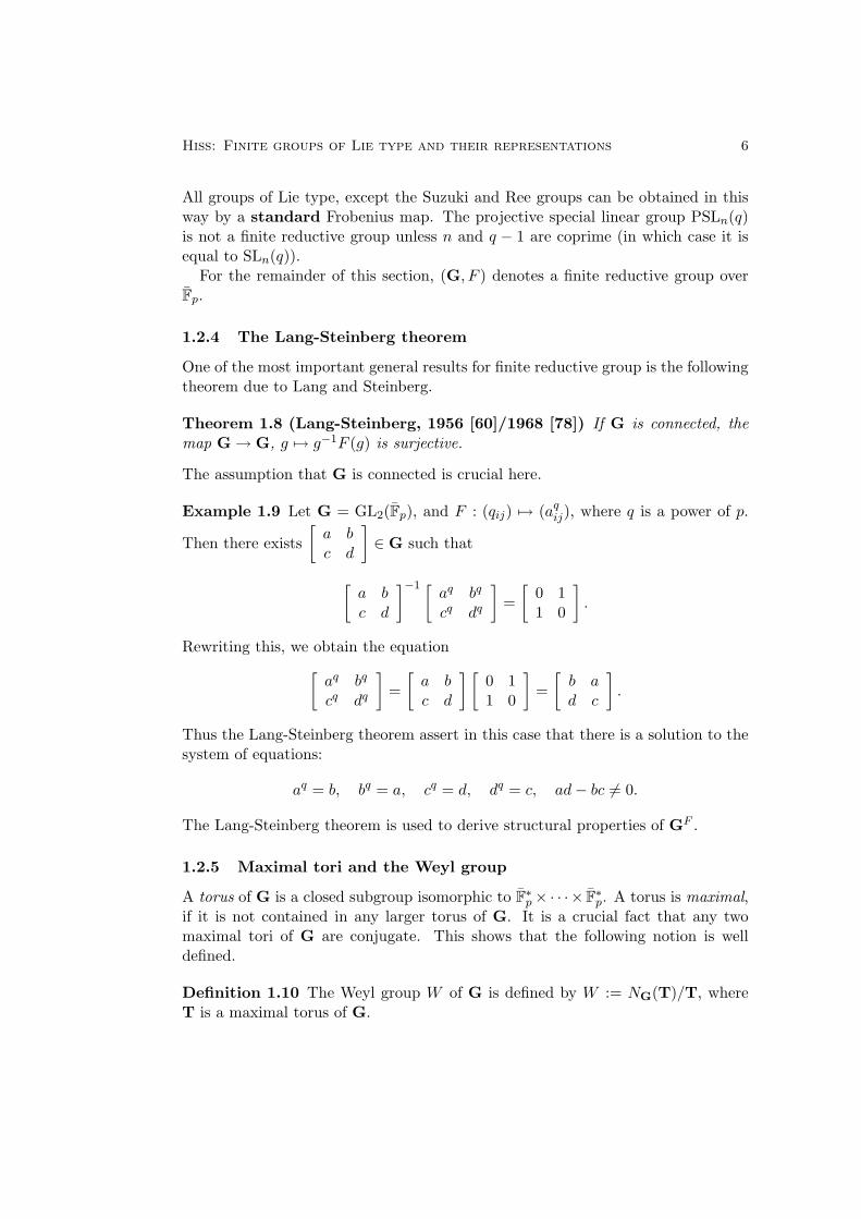
1.2.4 The Lang-Steinberg theorem

One of the most important general results for finite reductive group is the followingtheorem due to Lang and Steinberg.

Theorem 1.8 (Lang-Steinberg, 1956 [60]/1968 [78]) If G is connected, themap G→ G, g 7→ g−1F (g) is surjective.

The assumption that G is connected is crucial here.

Example 1.9 Let G = GL2(Fp), and F : (qij) 7→ (aqij), where q is a power of p.

Then there exists[

a bc d

]∈ G such that

[a bc d

]−1 [aq bq

cq dq

]=

[0 11 0

].

Rewriting this, we obtain the equation[aq bq

cq dq

]=

[a bc d

] [0 11 0

]=

[b ad c

].

Thus the Lang-Steinberg theorem assert in this case that there is a solution to thesystem of equations:

aq = b, bq = a, cq = d, dq = c, ad− bc 6= 0.

The Lang-Steinberg theorem is used to derive structural properties of GF .

1.2.5 Maximal tori and the Weyl group

A torus of G is a closed subgroup isomorphic to F∗p× · · ·× F∗p. A torus is maximal,if it is not contained in any larger torus of G. It is a crucial fact that any twomaximal tori of G are conjugate. This shows that the following notion is welldefined.

Definition 1.10 The Weyl group W of G is defined by W := NG(T)/T, whereT is a maximal torus of G.


Example 1.11 (1) Let G = GLn(Fp) and T the group of diagonal matrices. ThenT is a maximal torus of G, NG(T) is the group of monomial matrices, and W =NG(T)/T can be identified with the group of permutation matrices, i.e. W ∼= Sn.

(2) Next let G = SO2m+1(Fp) as defined in Example 1.2. Then

T := {diag[t1, . . . , tm, 1, t−1m , . . . , t−1

1 | ti ∈ F∗p, 1 ≤ i ≤ m}

is a maximal torus of G.For 1 ≤ i ≤ m− 1 let si be the permutation matrix corresponding to the double

transposition (i, i + 1)(m− i,m− i + 1). Put

sm :=

I 0 0 0 00 0 0 1 00 0 −1 0 00 1 0 0 00 0 0 0 I

,

where I denotes the identity matrix of degree m− 1. Then s1, . . . , sm are elementsof NG(T), and the cosets si := siT ∈ W , 1 ≤ i ≤ m, generate W , which is thus aCoxeter group of type Bm (see below).

1.2.6 Maximal tori of finite reductive groups

A maximal torus of (G, F ) is a finite reductive group (T, F ), where T is an F -stable maximal torus of G. A maximal torus of G = GF is a subgroup T of theform T = TF for some maximal torus (T, F ) of (G, F ).

Example 1.12 A Singer cycle in GLn(q) is an irreducible cyclic subgroup ofGLn(q) of order qn − 1. We will show below that a Singer cycle is a maximaltorus of GLn(q).

The maximal tori of (G, F ) are classified (up to conjugation in G) by F -conjugacyclasses of W . These are the orbits in W under the action v.w := vwF (v)−1,v, w ∈W .

1.2.7 The classification of maximal tori

Let T be an F -stable maximal torus of G, W = NG(T)/T.Let w ∈ W , and w ∈ NG(T) with w = wT. By the Lang-Steinberg theorem,

there is g ∈ G such that w = g−1F (g). One checks that gT is F -stable, andso (gT, F ) is a maximal torus of (G, F ). (Indeed, F (gT) = F (g)F (T)F (g)−1 =g(wTw−1)g−1 = gT since w ∈ NG(T).)

The map w 7→ (gT, F ) induces a bijection between the set of F -conjugacy classesof W and the set of G-conjugacy classes of maximal tori of (G, F ). For more detailssee [10, Section 3.3].

We say that gT is obtained from T by twisting with w.


1.2.8 The maximal tori of GLn(q)

Let G = GLn(Fp) and F = Fq a standard Frobenius morphism, where q is a powerof p.

Then F acts trivially on W = Sn, i.e. the maximal tori of G = GLn(q) areparametrised by partitions of n. If λ = (λ1, . . . , λl) is a partition of n, we write Tλ

for the corresponding maximal torus. We have

|Tλ| = (qλ1 − 1)(qλ2 − 1) · · · (qλl − 1).

Each factor qλi − 1 of |Tλ| corresponds to a cyclic direct factor of Tλ of this order.This follows form the considerations in the next subsection.

1.2.9 The structure of the maximal tori

Let T′ be an F -stable maximal torus of G, obtained by twisting the reference torusT with w = wT ∈ W . This means that there is g ∈ G with g−1F (g) = w andT′ = gT. Then

T ′ = (T′)F ∼= TwF := {t ∈ T | t = wF (t)w−1}.

Indeed, for t ∈ T we have gtg−1 = F (gtg−1) [= F (g)F (t)F (g)−1] if and only ift ∈ TwF .

Example 1.13 Let G = GLn(Fp), and T the group of diagonal matrices. Letw = (1, 2, . . . , n) be an n-cycle. Then

TwF = {diag[t, tq, . . . , tqn−1

] | t ∈ Fp, tqn−1 = 1},

and so TwF is cyclic of order qn − 1. It also follows that the maximal torus of Gcorresponding to w acts irreducibly on Fn

q and thus is a Singer cycle. On the otherhand, a maximal torus of G corresponding to an element of W not conjugate to wacts reducibly on V since it lies in a proper Levi subgroup. Since every semisimpleelement of G, in particular a generator of a Singer cycle, lies in some maximal torusof G, it follows that a a Singer cycle is indeed a maximal torus.

1.3 BN-pairs

The following axiom system was introduced by Jacques Tits to allow a uniformtreatment of groups of Lie type, not necessarily finite ones.

1.3.1 BN-pairs

We begin by defining what it means that a group has a BN -pair.

Definition 1.14 Let G be a group. The subgroups B and N of the group G forma BN -pair, if the following axioms are satisfied:

(1) G = 〈B,N〉;


(2) T := B ∩N is normal in N ;(3) W := N/T is generated by a set S of involutions;(4) If s ∈ N maps to s ∈ S (under N →W ), then sBs 6= B;(5) For each n ∈ N and s as above, (BsB)(BnB) ⊆ BsnB ∪BnB.

The group W = N/T is called the Weyl group of the BN -pair of G. It is a Coxetergroup with Coxeter generators S.

1.3.2 Coxeter groups

Let M = (mij)1≤i,j≤r be a symmetric matrix with mij ∈ Z∪{∞} satisfying mii = 1and mij > 1 for i 6= j. The group

W := W (M) :=⟨s1, . . . , sr | (sisj)mij = 1(i 6= j), s2

i = 1⟩group

(where the relation (sisj)mij = 1 is omitted if mij = ∞), is called the Coxetergroup of M , the elements s1, . . . , sr are the Coxeter generators of W .

The relations (sisj)mij = 1 (i 6= j) are called the braid relations. In view ofs2i = 1, they can be written as

sisjsi · · · = sjsisj · · · mij factors on each side.

The matrix M is usually encoded in a Coxeter diagram, a graph with nodes cor-responding to 1, . . . , r, and with number of edges between nodes i 6= j equal tomij − 2.

Example 1.15 The involutions si introduced in Example 1.11(2) satisfy the rela-tions s2

i = 1 for 1 ≤ i ≤ m, (sisi+1)3 = 1 for 1 ≤ i ≤ m − 1 and (sm−1sm)4 = 1.All other pairs of the si commute. The matrix encoding these relations is called aCoxeter matrix of type Bm. Its Coxeter diagram is as follows.

Bm: f f f f f. . .m m− 1 2 1

1.3.3 The BN-pair of GLn(k) and of SOn(k)

Let k be a field and G = GLn(k). Then G has a BN -pair with:• B the group of upper triangular matrices;• N the group of monomial matrices;• T = B ∩N the group of diagonal matrices;• W = N/T ∼= Sn the group of permutation matrices.

Let n = 2m + 1 be odd and let SOn(k) = {g ∈ SLn(k) | gtrJg = J} ≤ GLn(k) bethe orthogonal group. If B, N are as above for GLn(k), then

B ∩ SOn(k), N ∩ SOn(k)

is a BN -pair of SOn(k). (This would not have been the case had we defined SOn(k)with respect to an orthonormal basis as SOn(k) = {g ∈ SLn(k) | gtrg = I}.) UsingExamples 1.11 and 1.15 we see that the Weyl group of SOn(k) is a Coxeter groupof type Bm.


1.3.4 Split BN-pairs of characteristic p

Let G be a group with a BN -pair (B,N). This is said to be a split BN -pair ofcharacteristic p, if the following additional hypotheses are satisfied:

(6) B = UT with U = Op(B), the largest normal p-subgroup of B, and T acomplement of U .

(7)⋂

n∈N nBn−1 = T . (Recall T = B ∩N .)

Example 1.16 (1) A semisimple algebraic group G over Fp and a finite group ofLie type of characteristic p have split BN -pairs of characteristic p.

In G one chooses a maximal torus T and a maximal closed connected solublesubgroup B of G containing T. Such a B is called a Borel subgroup of G. Then Band NG(T) form a split BN -pair of G of characteristic p.

(2) If G = GLn(Fp) or GLn(q), q a power of p, then U is the group of uppertriangular unipotent matrices. In the latter case, U is a Sylow p-subgroup of G.

1.3.5 Parabolic subgroups and Levi subgroups

Let G be a group with a split BN -pair of characteristic p. Any conjugate of B iscalled a Borel subgroup of G. A parabolic subgroup of G is one containing a Borelsubgroup.

Let P ≤ G be a parabolic subgroup. Then

P = UP L = LUP (1)

such that UP = Op(P ) is the largest normal p-subgroup of P , and L is a complementto UP in P . The decomposition (1) is called a Levi decomposition of P , and L is aLevi complement of P , and a Levi subgroup of G.

A Levi subgroup is itself a group with a split BN -pair of characteristic p.

1.3.6 Examples for parabolic subgroups

In classical groups, parabolic subgroups are the stabilisers of isotropic subspaces.Let G = GLn(q), and (λ1, . . . , λl) a partition of n. Then

P =

GLλ1(q) ? ?

. . . ?GLλl

(q)

is a typical parabolic subgroup of G. A corresponding Levi subgroup is

L =

GLλ1(q)

. . .GLλl

(q)

∼= GLλ1(q)× · · · ×GLλl

(q).

If B denotes, once again, the group of upper triangular matrices in G, then a Levidecomposition of B is given by B = UT with T the diagonal matrices and U theupper triangular unipotent matrices.


1.3.7 The Bruhat decomposition

Let G be a group with a BN -pair. Then

G =⋃

w∈W

BwB (2)

(we write Bw := Bw if w ∈ N maps to w ∈ W under N → W ). The disjointunion (2) of G into B,B-double cosets, is called the Bruhat decomposition of G.(The Bruhat decomposition for GLn(k) follows from the Gaussian algorithm.)

Now suppose that the BN -pair is split, B = UT = TU . Let w ∈ W . ThenwT = Tw since T � N , and so BwB = BwU . Moreover, there is a subgroupUw ∈ U such that BwU = BwUw, with “uniqueness of expression”. This meansthat every element g ∈ BwUw can be written in a unique way as g = bwu withb ∈ B and u ∈ Uw. If furthermore, G is finite, this implies

|G| = |B|∑

w∈W

|Uw|.

1.3.8 The orders of the finite groups of Lie type

Let G be a finite group of Lie type of characteristic p. Then G has a split BN -pairof characteristic p. Thus

|G| = |B|∑

w∈W

|Uw|.

Assume for simplicity that G = GF for a standard Frobenius map F = Fq. Then|Uw| = q`(w), where `(w) is the length of w ∈W , i.e. the length of the shortest wordin the Coxeter generators S of W expressing w.

By theorems of Solomon (1966, [72]) and Steinberg (1968, [78]),

∑w∈W

q`(w) =r∏

i=1

qdi − 1q − 1

,

where d1, . . . , dr are the degrees of the basic polynomial invariants of W . This givesthe formulae for |G| displayed in Example 1.3. An analogous, but slightly morecomplicated argument yields the order formulae for the twisted groups. For detailssee [9, Chapter 14].

2 Representations in defining characteristic

In this section we introduce the fundamental problems in the representation theoryof finite groups of Lie type in the defining characteristic case. A comprehensiveaccount of the knowledge in this area is given in Jantzen’s monograph [57]. Seealso [50].


2.1 Classification of representations

2.1.1 A fundamental problem in representation theory

Let G be a finite group and k a field. It is a fundamental fact that there areonly finitely many irreducible k-representations of G up to equivalence. This sug-gests the problem of classifying all irreducible representations of G over k. Moreambitious is the following fundamental task:

Classify all irreducible representations of all finite simple groups overall fields.

As already mentioned, “most” finite simple groups are groups of Lie type, and asa first step towards a classification of their irreducible representations one needsto find labels for these, their degrees, etc. It is useful to begin with the case ofalgebraically closed fields k. Instead of talking of representations we also use theequivalent language of kG-modules.

2.1.2 Three Cases

In the following, let G = GF be a finite reductive group. Recall that G is aconnected reductive algebraic group over Fp and that F is a Frobenius morphismof G. Let k be algebraically closed with char(k) = ` ≥ 0. It is natural to distinguishthree cases:

1. ` = p (usually k = Fp); defining characteristic2. ` = 0; ordinary representations3. ` > 0, ` 6= p; non-defining characteristic

In this section we consider Case 1, and the remaining two sections are devoted toCases 2 and 3.

2.2 Representations of (finite) reductive groups

2.2.1 A rough survey

Let us begin with a rough survey. Let k = Fp and let (G, F ) be a finite reductivegroup over k.

By a k-representation of G we understand an algebraic homomorphism, i.e. ahomomorphism of groups that is also a morphism of algebraic varieties. We listsome fundamental facts about the classification of irreducible k-representations ofG and of G = GF .

1. An irreducible k-representation of G has finite degree.2. The irreducible k-representations of G are classified by dominant weights, i.e.

we have labels for these irreducible k-representations.3. Under a natural condition on G, every irreducible k-representation of G =

GF is the restriction of an irreducible k-representation of G to G.We thus have to discuss the following questions. What are dominant weights?Which irreducible representations of G restrict to irreducible representations of G?


2.2.2 Character group and cocharacter group

For the remainder of this lecture, let G be a connected reductive algebraic groupover k = Fp and let T be a maximal torus of G. (All of these are conjugate.)Recall that T ∼= k∗ × k∗ × · · · × k∗. The number r of factors is an invariant of G,the rank of G.

Put X := X(T) := Hom(T, k∗). Again, Hom refers to algebraic homomorphismsof algebraic groups. Then X is an abelian group which we write additively. ThusX ∼=

⊕r1 Hom(k∗, k∗). Now Hom(k∗, k∗) ∼= Z, so X is a free abelian group of rank r.

(Indeed, every χ ∈ Hom(k∗, k∗) is of the form χ(t) = tz for some z ∈ Z.) Similarly,Y := Y (T) := Hom(k∗,T) is free abelian of rank r.

The groups X and Y are called the character group and cocharacter group,respectively. There is a natural duality X × Y → Z, (χ, γ) 7→ 〈χ, γ〉, defined byχ ◦ γ ∈ Hom(k∗, k∗) ∼= Z.

2.2.3 The character groups and cocharacter groups of GLn(k) and SLn(k)

Let G = GLn(k). Take

T := {diag[t1, t2, . . . , tn] | t1, . . . , tn ∈ k∗},

the maximal torus of diagonal matrices. (Thus GLn(k) has rank n.) The charactergroup X has basis ε1, . . . , εn with

εi(diag[t1, t2, . . . , tn]) = ti.

The cocharacter group Y has basis ε′1, . . . ε′n with

ε′i(t) = diag[1, . . . 1, t, 1, · · · , 1],

where the t is on position i. Clearly, {εi} and {ε′i} are dual with respect to thepairing 〈−,−〉.

Now let G = SLn(k) with k = Fp. Take

T := {diag[t1, t2, . . . , tn] | t1, . . . , tn ∈ k∗, t1t2 · · · tn = 1} ,

the maximal torus of diagonal matrices. (Thus SLn(k) has rank n − 1.) Thecharacter group X has basis ε1, . . . , εn−1 with

εi(diag[t1, t2, . . . , tn]) = ti.

Y has basis ε′1, . . . ε′n−1 with

ε′′i (t) = diag[1, . . . 1, t, 1, · · · , 1, t−1],

where the t is on position i. Clearly, {εi} and {ε′′i } are dual with respect to thepairing 〈−,−〉.


2.2.4 Roots and coroots

Let B be a Borel subgroup of G containing T. Then B = UT with U � B andU ∩T = {1}. (Recall that G has a split BN -pair of characteristic p.)

The minimal subgroups of U normalised by T are called root subgroups. A rootsubgroup is isomorphic to Ga := (k, +). The action of T on a root subgroupgives rise to a homomorphism T → Aut(Ga). Since Aut(Ga) ∼= k∗, we obtainan element of X. The characters obtained this way are the positive roots of Gwith respect to T and B. The set of positive roots is denoted by Φ+, and the setΦ := Φ+ ∪ (−Φ+) ⊂ X is the root system of G.

One can also define a set Φ∨ ⊂ Y of coroots of G with respect to T and B.Indeed, let α ∈ Φ+ and let Uα ≤ U be the corresponding root subgroup. Thenthere is a homomorphism ϕ : SL2(k)→ G with

ϕ

{[1 a0 1

]| a ∈ k

}= Uα,

and

ϕ

{[a 00 a−1

]| a ∈ k∗

}≤ T.

Now define α∨ ∈ Y = Hom(k∗,T) by α∨(a) := ϕ

{[a 00 a−1

]}for a ∈ k∗.

2.2.5 The roots and the coroots of GLn(k) and of SLn(k) and the rootsof SO2m+1(k)

Let G = GLn(k) and T the maximal torus of diagonal matrices. We choose B asgroup of upper triangular matrices. Then U is the subgroup of upper triangularunipotent matrices.

The root subgroups are the groups

Uij := {In + aIij | a ∈ k}, 1 ≤ i < j ≤ n,

where Iij denotes the elementary matrix with 1 on position (i, j) and 0 elsewhere.The positive root αij determined by Uij equals εi − εj .

Indeed, if t = diag[t1, . . . , tn], then t(In +aIij)t−1 = In + tit−1j aIij . On the other

hand, (εi − εj)(t) = tit−1j . We have

Φ = {αij | αij = εi − εj , 1 ≤ i 6= j ≤ n}

andΦ∨ = {α∨ij | α∨ij = ε′i − ε′j , 1 ≤ i 6= j ≤ n}.

Note that ZΦ and ZΦ∨ have rank n− 1.Now let G = SLn(k) and T be as in 2.2.3 and let B and U be as above. The

root subgroups are the same as for GLn(q). The positive root αij determined byUij equals εi − εj if j 6= n, and αin = εi +

∑n−1j=1 εj . We have α∨ij = ε′′i − ε′′j for


i < j < n and α∨in = ε′′i for i < n. In this example X/ZΦ is cyclic of order n, andY = ZΦ∨.

Finally, assume that n = 2m + 1 and p are odd, and let G = SOn(k). Let T, Band U denote, respectively, the group of diagonal, upper triangular and upper trian-gular unipotent matrices contained in G. Then T is as in Example 1.11. Clearly, abasis of X = X(T) consists of ε1, . . . , εm with εi(diag[t1, . . . , tm, 1, t−1

m , . . . , t−11 ]) =

ti, 1 ≤ i ≤ m. The root subgroups are the groups

Uij := {In + aIij − aI2m−j+2,2m−i+2 | a ∈ k}, 1 ≤ i < j ≤ m,

together with

U′ij = {In + aIi,2m−j+2 − aIj,2m−i+2 | a ∈ k}, 1 ≤ i < j ≤ m,

and

Ui = {In + aIi,m+1 − aIm+1,2m−i+2 − a2/2Ii,2m−i+2}, 1 ≤ i ≤ m.

The positive roots αij and α′ij determined by Uij and U′ij , respectively, equal εi−εj

and εi + εj , respectively. Moreover, the positive roots determined by Ui equals εi,1 ≤ i ≤ m. In this case X = ZΦ.

2.2.6 The root datum

The quadruple (X, Φ, Y,Φ∨) constructed from G satisfies:1. X and Y are free abelian groups of the same rank and there is a duality

X × Y → Z, (χ, γ) 7→ 〈χ, γ〉.2. Φ and Φ∨ are finite subsets of X and of Y , respectively, and there is a bijection

Φ→ Φ∨, α 7→ α∨.3. For α ∈ Φ we have 〈α, α∨〉 = 2. Denote by sα the “reflection” of X defined

bysα(χ) = χ− 〈χ, α∨〉α,

and let s∨α be its adjoint (s∨α(γ) = γ − 〈α, γ〉α∨).Then sα(Φ) = Φ and s∨α(Φ∨) = Φ∨.

A quadruple (X, Φ, Y,Φ∨) as above is called a root datum.The algebraic group G is determined by its root datum (and p) up to isomor-

phism. More precisely, we have the following. Suppose that G and G1 are con-nected reductive groups over Fp with Borel subgroups B = UT and B1 = U1T1,respectively. Let, furthermore, ΓG := (X, Φ, Y,Φ∨) and ΓG1 := (X1,Φ1, Y1,Φ∨

1 ) bethe corresponding root data. There is an obvious notion of isomorphism of rootdata.

Theorem 2.1 (Isomorphism theorem) Suppose that f : ΓG1 → ΓG is an iso-morphism of root data. Then there exists an isomorphism ϕ : G→ G1 of algebraicgroups with ϕ(T) = T1. Moreover, ϕ is uniquely determined up to conjugationin T.

An exact statement and a proof of the isomorphism theorem can be found inSpringer’s book [73, Thm. 9.6.2].


2.2.7 The Weyl group

The Weyl group W = NG(T)/T acts on X and we have

W ∼= 〈sα | α ∈ Φ〉 ≤ Aut(X).

Suppose that G is semisimple. Then rankX = rank ZΦ. In this case Φ is a rootsystem in V := X⊗ZR and W is its Weyl group (where V is equipped with an innerproduct (−,−) satisfying 〈β, α∨〉 = 2(β, α)/(α, α) for all α, β ∈ Φ). Moreover, Wis a Coxeter group with Coxeter generators {sα | α ∈ Π}, where Π ⊂ Φ+ is a baseof Φ. Note that Π is uniquely determined by this property. Indeed, Π consists ofthose elements of Φ+ which cannot be written as sums of elements of Φ+.

2.2.8 Weight spaces

Let M be a finite-dimensional algebraic kG-module. This means that the k-re-presentation of G afforded by M is algebraic. For λ ∈ X = X(T) = Hom(T, k∗)put

Mλ := {v ∈M | tv = λ(t)v for all t ∈ T}.

If Mλ 6= {0}, then λ is called a weight of M and Mλ is the corresponding weightspace. (Thus Mλ is a simultaneous eigenspace for all t ∈ T.) It is a crucial fact,that M is a direct sum of its weight spaces, i.e.

M =⊕λ∈X

Mλ.

This follows from the fact that the elements of T act as commuting semisimplelinear operators on M .

2.2.9 Dominant weights and simple modules

The elements of the set

X+ := {λ ∈ X | 0 ≤ 〈λ, α∨〉 for all α ∈ Φ+} ⊂ X

are called the dominant weights of T (with respect to Φ+).

Example 2.2 Let G = GLn(Fp) and let T be the maximal torus of diagonalmatrices. Use the notation for the roots and coroots of G from subsubsection 2.2.5.

An element λ ∈ X is of the form λ =∑n

i=1 λiεi with λi ∈ Z for all 1 ≤ i ≤ n.Now λ ∈ X+ if and only if 〈λ, α∨ij〉 ≥ 0 for all 1 ≤ i < j ≤ n. Since α∨ij = ε′i − ε′j ,this is the case if and only if λi − λj ≥ 0 for all 1 ≤ i < j ≤ n. It follows that X+

corresponds to the ordered sequences λ1 ≥ λ2 ≥ . . . ≥ λn of integers.

We order X by µ ≤ λ if and only if λ− µ is a sum of roots in Π. We then havethe following classification of the simple kG-modules.


Theorem 2.3 (Chevalley, late 1950s, cf. [12]) (1) For each λ ∈ X+ there isa simple kG-module L(λ).

(2) dim L(λ)λ = 1. If µ is a weight of L(λ), then µ ≤ λ. (Consequently, λ iscalled the highest weight of L(λ).)

(3) If M is a simple kG-module, then M ∼= L(λ) for some λ ∈ X+.

The dimensions of the dim L(λ) are not known except for some special cases.

2.2.10 The natural and the adjoint representations of GLn(k)

Let G = GLn(k). Let M := kn be the natural module of kG. Then the weights ofM are the εi, 1 ≤ i ≤ n. The highest of these is ε1 (recall that εi − εj ∈ Φ+ fori < j). Thus M = L(ε1).

Next, let M := {x ∈ kn×n | tr(x) = 0}. Then M is a simple kG-module byconjugation (the adjoint module). The weights of M are the roots αij and 0. Thehighest one of these is α1n = ε1 − εn. Thus M = L(ε1 − εn) = L(αin).

2.2.11 Steinberg’s tensor product theorem

For q = pm, put

X+q := {λ ∈ X | 0 ≤ 〈λ, α∨〉 < q for all α ∈ Π} ⊂ X+.

(Recall that Π ⊂ Φ+ is a base of Φ.) Let F = Fp denote the standard Frobeniusmorphism (aij) 7→ (ap

ij). If M is a kG-module, we put M [i] := M , with twistedaction g.v := F i(g).v, g ∈ G, v ∈M .

Theorem 2.4 (Steinberg’s tensor product theorem, [76]) For λ ∈ X+q write

λ =∑m−1

i=0 piλi with λi ∈ X+p . (This is called the p-adic expansion of λ.) Then

L(λ) = L(λ0)⊗k L(λ1)[1] ⊗k · · · ⊗k L(λm−1)[m−1].

Thus it suffices to determine the dimensions of the simple modules Lλ for λ in thefinite set X+

p . The next theorem gives a classification of the simple modules forthe finite groups of Lie type.

Theorem 2.5 (Steinberg, [76]) If λ ∈ X+q , then the restriction of L(λ) to G =

GF mis simple. If G is simply connected, i.e. Y = ZΦ∨, then every simple kG-

module arises this way.

2.2.12 The irreducible representations of SL2(k)

Let G = SL2(k). Then G acts as group of k-algebra automorphisms on the poly-nomial ring k[x1, x2] in two variables, the action being defined by:[

a bc d

] [x1

x2

]=

[ax1 + bx2

cx1 + dx2

].


For j = 0, 1, . . . let Mj denote the set of homogeneous polynomials in k[x1, x2]of degree j. Then Mj is G-invariant, hence a kG-module, and dim Mj = j + 1.Moreover, Mj is a simple kG-module, in fact Mj = L(jε1), if 0 ≤ j < p. Ingeneral, write j = j0 + pj1 + · · · + pmjm with 0 ≤ ji < p. Then, by Steinberg’stensor product theorem, L(jε1) = Mj0 ⊗k M

[1]j1⊗k · · · ⊗k M

[m]jm

.Thus SL2(p) has exactly the simple modules M0, . . . ,Mp−1 of dimensions 1, . . . , p.

This description of the p-modular irreducible representations of SL2(q) (for powersq of p) is due to Brauer and Nesbitt [6].

2.2.13 Weyl modules

From now on assume that G is simply connected, i.e. Y = ZΦ∨. For each λ ∈ X+,there is a distinguished finite-dimensional kG-module V (λ). These V (λ) are calledWeyl modules.

The Weyl modules are constructed via reduction modulo p. Let Φ be the rootsystem of G and let g be the semisimple Lie algebra over C with root system Φ.For λ ∈ X+, let V (λ)C be a simple g-module with highest weight λ. This hasa suitable Z-form V (λ)Z. Then V (λ) := k ⊗Z V (λ)Z can be equipped with thestructure of a kG-module.

This construction generalises the construction of the Chevalley groups as groupsof automorphisms on a Z-form of their adjoint module.

2.2.14 Formal characters

Let M be a finite-dimensional kG-module. Recall that

M =⊕λ∈X

Mλ.

Clearly, dim M can be recovered by the vector (dim Mλ)λ∈X . It is convenient toview this as an element of ZX, the group ring of X over Z. We introduce a Z-basiseλ, λ ∈ X, of ZX with eλeµ = eλ+µ.

Definition 2.6 The formal character of M is the element

chM :=∑λ∈X

dim Mλ eλ

of ZX.

2.2.15 Characters of Weyl modules

The characters of the Weyl modules V (λ) can be computed from Weyl’s characterformula, which is not reproduced here. In particular, dim V (λ) is known.

Put aλ,µ := [V (λ):L(µ)] := multiplicity of L(µ) as a composition factor of V (λ).It is known that aλ,λ = 1, and if aλ,µ 6= 0, then µ ≤ λ. We obviously have

chV (λ) = chL(λ) +∑µ<λ

aλ,µ chL(µ).


Once the aλ,µ are known, chL(λ) and thus dim L(λ) can be computed recursivelyfrom chV (µ) with µ ≤ λ (there are only finitely many such µ).

2.3 Lusztig’s conjecture

Lusztig’s conjecture proposes a formula to compute the multiplicities aλ,µ in certaincases. The conjecture is in terms of Kazhdan-Lusztig polynomials.

2.3.1 The Iwahori-Hecke algebra

Let M = (mij)1≤i,j≤r be a symmetric matrix with mij ∈ Z∪{∞} satisfying mii = 1and mij > 1 for i 6= j. Recall that

W =⟨s1, . . . , sr | (sisj)mij = 1(i 6= j), s2

i = 1⟩group ,

is the Coxeter group of M . Let A be a commutative ring and v ∈ A. The algebra

HA,v(W ) :=⟨Ts1 , . . . , Tsr | T 2

si= v1 + (v − 1)Tsi , braid rel’s

⟩A-alg.

is called the Iwahori-Hecke algebra of W over A with parameter v. The braidrelations are

TsiTsjTsi · · · = TsjTsiTsj · · · (mij factors on each side).

It is a well known fact that HA,v(W ) is a free A-algebra with A-basis Tw, w ∈W .Note that HA,1(W ) ∼= AW , so that HA,v(W ) is a deformation of AW , the group

algebra of W over A.

2.3.2 Kazhdan-Lusztig polynomials

Let W be a Coxeter group as above and let ≤ denote the Bruhat order on W . Letv be an indeterminate, put A := Z[v, v−1] and u := v2.

There is an involution ι on HA,u(W ) determined by ι(v) = v−1 and ι(Tw) =(Tw−1)−1 for all w ∈ W . (The square root v of u is needed in order for Tw to beinvertible in HA,u(W ).)

Theorem 2.7 (Kazhdan-Lusztig, [58]) There is a unique basis C ′w, w ∈ W of

HA,u(W ) such that(1) ι(C ′

w) = C ′w for all w ∈W ;

(2) C ′w = v−`(w)

∑y≤w Py,wTw with Pw,w = 1, Py,w ∈ Z[u], deg Py,w ≤ (`(w) −

`(y)− 1)/2 for all y < w ∈W .

The Py,w ∈ Z[u], y ≤ w ∈W , are called the Kazhdan-Lusztig polynomials of W .


2.3.3 The affine Weyl group

Recall that the Weyl group W acts on X as a group of linear transformations. Letρ := 1

2

∑α∈Φ+ α, and define the dot-action of W as follows:

w.λ := w(λ + ρ)− ρ, λ ∈ X, w ∈W.

DefineWp = 〈sα,z | α ∈ Φ+, z ∈ Z〉.

Here, sα,z(λ) = sα.λ+zpα is an affine reflection of X. Then Wp is a Coxeter group,called the affine Weyl group.

Each Wp-orbit on X contains a unique element in C := {λ ∈ X | 0 ≤ 〈λ +ρ, α∨〉 ≤ p for all α ∈ Φ+}.

2.3.4 Lusztig’s conjecture

Let λ0 ∈ X with 0 < 〈λ0 + ρ, α∨〉 < p for all α ∈ Φ+. Such a λ0 only exists ifp ≥ h := h(W ) := max{〈ρ, α∨〉 | α ∈ Φ+} + 1). The following theorem combinesspecial cases of the linkage principle and the translation principle.

Theorem 2.8 (Humhreys, 1971, [48]; Jantzen, 1974, [56]) For w ∈Wp suchthat w.λ0 ∈ X+

p we have chL(w.λ0) =∑

w′ bw,w′ chV (w′.λ0), with w′ ∈ Wp suchthat w′.λ0 ≤ w.λ0 and w′.λ0 ∈ X+. The bw,w′ are independent of λ0.

For p ≥ h, the computation of chL(λ) for any λ ∈ X+ can be reduced to one ofthese cases. In the following formulation of Lusztig’s conjecture, let w0 denote thelongest element in W ≤Wp.

Conjecture 2.9 (Lusztig’s conjecture, 1980, [64]) The numbers bw,w′ are giv-en by bw,w′ = (−1)`(w)+`(w′)Pw0w′,w0w(1), in particular, the bw,w′ are also indepen-dent of p.

Theorem 2.10 (Andersen-Jantzen-Soergel, [2]) Lusztig’s conjecture is trueprovided p >> 0.

3 Representations in characteristic zero

Here we describe, to some extent, the ordinary representation theory of finite groupsof Lie type. The material in this section can be found in the textbooks [10, 15] byCarter and Digne-Michel.

3.1 Harish-Chandra theory

In the following, unless otherwise said, let G be a finite reductive group of charac-teristic p. Also, k denotes an algebraically closed field of characteristic ` ≥ 0. InSection 2 we have considered the situation ` = p. In this section we will mainly,but not exclusively, investigate the case ` = 0.


Recall that there is a distinguished class of subgroups of G, the parabolic sub-groups. One way to describe them is through the concept of split BN -pairs ofcharacteristic p. A parabolic subgroup P has a Levi decomposition P = LU ,where U = Op(P )�P is the unipotent radical of P , and L a Levi complement of Uin P , i.e. L is a Levi subgroup of G. Levi subgroups of G resemble G; in particular,they are again groups of Lie type. Inductively, we may use the representations ofthe Levi subgroups to obtain information about the representations of G. This isthe idea behind Harish-Chandra theory.

3.1.1 Harish-Chandra induction

Assume from now on that ` 6= p. Let L be a Levi subgroup of G, and M a kL-module. View M as a kP -module via π : P → L (a.v := π(a).v for v ∈M , a ∈ P ).Put

RGL (M) := {f : G→M | a.f(b) = f(ab) for all a ∈ P, b ∈ G} .

This construction is analogous to the definition of modular forms in number theory.Then RG

L (M) is a kG-module, called Harish-Chandra induced module. Theaction of G is given by right multiplication in the arguments of the functions inRG

L (M): g.f(b) := f(bg), g, b ∈ G, f ∈ RGL (M).

It is an important fact that RGL (M) is independent of the choice of P with P → L.

In the case of ` > 0, this result is due to Dipper-Du [18], and, independently, toHowlett-Lehrer [47].

3.1.2 Centraliser algebras

With L and M as before, put

H(L,M) := EndkG(RGL (M)).

Then H(L,M) is the centraliser algebra (or Hecke algebra) of the kG-moduleRG

L (M), i.e.

H(L,M) ={γ ∈ Endk(RG

L (M)) | γ(g.f) = g.γ(f) for all g ∈ G, f ∈ RGL (M)

}.

The centraliser algebra H(L,M) is used to analyse the submodules and quotientsof RG

L (M).

3.1.3 Iwahori’s example

The following example is a special case of the results of Iwahori [52]. It marksthe first appearance of the Iwahori-Hecke algebra in the representation theory offinite groups. Suppose that ` = 0. Let G = GLn(q), L = T , the group of diagonalmatrices, M the trivial kL-module. Then

H(L,M) = Hk,q(Sn),


the Iwahori-Hecke algebra over k with parameter q associated to the Weyl group Sn

of G. Recall the k-algebra presentation of Hk,q(Sn):⟨T1, . . . , Tn−1 | braid relations , T 2

i = q1k + (q − 1)Ti

⟩k-algebra ,

with the braid relations

TiTi+1Ti = Ti+1TiTi+1 (1 ≤ i ≤ n− 2).

3.1.4 Harish-Chandra classification

Let V be a simple kG-module. Then V is called cuspidal, if V is not a submoduleof RG

L (M) for some proper Levi subgroup L of G and some kL-module M . Harish-Chandra theory, i.e. Harish-Chandra induction and the concept of cuspidality yieldsthe following classification.

Theorem 3.1 (Harish-Chandra [40], Lusztig [63, 65], ` = 0; Geck-Hiss-Malle [36], ` > 0) There is a bijection

{V | V simple kG-module } /iso.l(L,M, θ) |

L Levi subgroup of GM simple, cuspidal kL-module

θ irreducible k-representation of H(L,M)

/conj.

This theorem allows to partition the isomorphism classes of the simple kG-modulesinto Harish-Chandra series. Two simple kG-modules lie in the same Harish-Chandra series, if and only if they arise from the same cuspidal pair (L,M), whereL is a Levi subgroup and M a simple, cuspidal kL-module.

3.1.5 Problems in Harish-Chandra theory

The above theorem leads to the following three fundamental tasks:(1) Determine the cuspidal pairs (L,M).(2) For each of these, “compute” H(L,M).(2) Classify the irreducible k-representations of H(L,M).

The state of the art in this program in case ` = 0 is mainly due to Lusztig (see[65]):

(1) Lusztig has constructed and classified the simple cuspidal kG-modules. Theyarise from etale cohomology groups of Deligne-Lusztig varieties.

(2) For each cuspidal pair (L,M) consider the ramification group

WG(L,M) := (NG(L,M) ∩N)L/L

(the subgroup N ≤ G here is the one from the BN -pair of G). If G = GF withZ(G) connected, then it turns out that WG(L,M) is a Coxeter group. More-over, the centraliser algebra H(L,M) is an Iwahori-Hecke algebra corresponding toWG(L,M).

(3) Furthermore, H(L,M) ∼= kWG(L,M). This is a consequence of the Titsdeformation theorem.


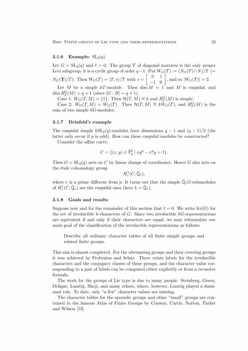
3.1.6 Example: SL2(q)

Let G = SL2(q) and ` = 0. The group T of diagonal matrices is the only properLevi subgroup; it is a cyclic group of order q−1. Put WG(T ) := (NG(T )∩N)/T (=

NG(T)/T ). Then WG(T ) = 〈T, s〉/T with s =[

0 1−1 0

], and so |WG(T )| = 2.

Let M be a simple kT -module. Then dim M = 1 and M is cuspidal, anddim RG

T (M) = q + 1 (since [G : B] = q + 1).Case 1: WG(T,M) = {1}. Then H(T,M) ∼= k and RG

T (M) is simple.Case 2: WG(T,M) = WG(T ). Then H(T,M) ∼= kWG(T ), and RG

T (M) is thesum of two simple kG-modules.

3.1.7 Drinfeld’s example

The cuspidal simple kSL2(q)-modules have dimensions q − 1 and (q − 1)/2 (thelatter only occur if p is odd). How can these cuspidal modules be constructed?

Consider the affine curve

C = {(x, y) ∈ F2p | xyq − xqy = 1}.

Then G = SL2(q) acts on C by linear change of coordinates. Hence G also acts onthe etale cohomology group

H1c (C, Qr),

where r is a prime different from p. It turns out that the simple QrG-submodulesof H1

c (C, Qr) are the cuspidal ones (here k = Qr).

3.1.8 Goals and results

Suppose now and for the remainder of this section that ` = 0. We write Irr(G) forthe set of irreducible k-characters of G. Since two irreducible kG-representationsare equivalent if and only if their characters are equal, we may reformulate ourmain goal of the classification of the irreducible representations as follows:

Describe all ordinary character tables of all finite simple groups andrelated finite groups.

This aim is almost completed. For the alternating groups and their covering groupsit was achieved by Frobenius and Schur. There exists labels for the irreduciblecharacters and the conjugacy classes of these groups, and the character value cor-responding to a pair of labels can be computed either explicitly or from a recursiveformula.

The work for the groups of Lie type is due to many people: Steinberg, Green,Deligne, Lusztig, Shoji, and many others, where, however, Lusztig played a domi-nant role. To date, only “a few” character values are missing.

The character tables for the sporadic groups and other “small” groups are con-tained in the famous Atlas of Finite Groups by Conway, Curtis, Norton, Parkerand Wilson [13].


3.2 Deligne-Lusztig theory

We begin this subsection by displaying an example of a generic character table.

3.2.1 The generic character table for SL2(q), q even

C1 C2 C3(a) C4(b)

χ1 1 1 1 1

χ2 q 0 1 −1

χ3(m) q + 1 1 ζam + ζ−am 0

χ4(n) q − 1 −1 0 −ξbn − ξ−bn

Here, the parameters a, b label conjugacy classes, and m,n label irreducible char-acters. The range of these parameters is as follows: a,m = 1, . . . , (q − 2)/2,b, n = 1, . . . , q/2. Moreover, the entries ζ and ξ are “generic roots of unity”,namely

ζ := exp(2π√−1

q − 1), ξ := exp(

2π√−1

q + 1).

The conjugacy classes C3(a) and C4(b) have representatives as follows[µa 00 µ−a

]∈ C3(a) (µ ∈ Fq a primitive (q − 1)th root of unity),

[νb 00 ν−b

]∈∼ C4(b) (ν ∈ Fq2 a primitive (q + 1)th root of unity).

(The symbol ∈∼ indicates that an element in class C4(b) is conjugate in GL2(F2) tothe element on the left hand side.) Specialising q to 4, gives the character table ofSL2(4) ∼= A5.

3.2.2 Deligne-Lusztig varieties

Let r be a prime different from p and put k := Qr. Let (G, F ) be a finite reductivegroup, G = GF . Deligne and Lusztig [14] construct for each pair (T, θ), where Tis an F -stable maximal torus of G, and θ ∈ Irr(TF ), a generalised character RG

T,θ

of G. (A generalised character of G is an element of Z[Irr(G)].)Let (T, θ) be a pair as above. Choose a Borel subgroup B = TU of G with Levi

subgroup T. (In general B is not F -stable.) Consider the Deligne-Lusztig varietyassociated to B,

XB = {g ∈ G | g−1F (g) ∈ U}.

This is an algebraic variety over Fp.


3.2.3 Deligne-Lusztig generalised characters

The finite groups G = GF and T = TF act on XB, and these actions commute.Thus the etale cohomology group H i

c(XB, Qr) is a Qr[G × T ]-module, and so itsθ-isotypic component H i

c(XB, Qr)θ is a QrG-module, whose character is denotedby ch H i

c(XB, Qr)θ.Only finitely many of the vector spaces H i

c(XB, Qr) are 6= 0. Now put

RGT,θ =

∑i

(−1)ich H ic(XB, Qr)θ.

Then RGT,θ is independent of the choice of B containing T.

3.2.4 Properties of Deligne-Lusztig characters

The above construction and the following facts are due to Deligne and Lusztig,[14].

Facts 3.2 Let (T, θ) be a pair as above. Then(4) RG

T,θ(1) = ±[G : T ]p′ .(2) If T is contained in an F -stable Borel subgroup B, then RG

T,θ = RGT (θ) is the

Harish-Chandra induced character.(3) If θ is in general position, i.e. NG(T, θ)/T = {1}, then ±RG

T,θ is an irreduciblecharacter.

(4) For χ ∈ Irr(G), there is a pair (T, θ) such that χ occurs in the (unique)expansion of RG

T,θ into Irr(G). (Recall that Irr(G) is a basis of Z[Irr(G)].)

3.2.5 Unipotent characters

Definition 3.3 (Deligne-Lusztig, [14]) A k-character χ of G is called unipo-tent, if χ is irreducible, and if χ occurs in RG

T,1 for some F -stable maximal torusT of G, where 1 denotes the trivial character of T = TF . We write Irru(G) for theset of unipotent characters of G.

The above definition of unipotent characters uses etale cohomology groups. So far,no elementary description known, except for GLn(q); see below. Lusztig classi-fied Irru(G) in all cases, independently of q. Harish-Chandra induction preservesunipotent characters, so it suffices to construct the cuspidal unipotent characters.

3.2.6 The unipotent characters of GLn(q)

Let G = GLn(q). Then Irru(G) = {χ ∈ Irr(G) | χ occurs in RGT (1)}. This is the

set of constituents in the permutation character with respect to the action on thecosets of the subgroup of upper triangular matrices. Moreover, there is a bijection

Pn ↔ Irru(G), λ↔ χλ,

where Pn denotes the set of partitions of n.


The degrees of the unipotent characters are “polynomials in q”:

χλ(1) = qd(λ) (qn − 1)(qn−1 − 1) · · · (q − 1)∏

h(λ)(qh − 1),

with a certain d(λ) ∈ N, and where h(λ) runs through the hook lengths of λ.

3.2.7 The degrees of the unipotent characters of GL5(q)

λ χλ(1)

(5) 1(4, 1) q(q + 1)(q2 + 1)(3, 2) q2(q4 + q3 + q2 + q + 1)(3, 12) q3(q2 + 1)(q2 + q + 1)(22, 1) q4(q4 + q3 + q2 + q + 1)(2, 13) q6(q + 1)(q2 + 1)(15) q10

3.3 Lusztig’s Jordan decomposition of characters

In this subsection we introduce Lusztig’s classification of the set of irreduciblecharacters of G, known as Jordan decomposition of characters.

3.3.1 Jordan decomposition of elements

An important concept in the classification of elements of a finite reductive groupis the Jordan decomposition of elements.

Since G ≤ GLn(Fp), every g ∈ G has finite order. Hence g has a uniquedecomposition as

g = su = us (3)

with u a p-element and s a p′-element. It follows from Linear algebra that u isunipotent, i.e. all eigenvalues of u are equal to 1, and s is semisimple, i.e. diagonal-isable.

The decomposition (3) is called the Jordan decomposition of g ∈ G. If g ∈ G =GF , then so are u and s.

3.3.2 Jordan decomposition of conjugacy classes

This yields a model classification for the classification of the irreducible charactersof G in case ` = 0 and, conjecturally, also in case 0 6= ` 6= p.

For g ∈ G with Jordan decomposition g = us = su, we write CGu,s for the

G-conjugacy class containing g. This gives a labelling

{conjugacy classes of G}l

{CGs,u | s semisimple, u ∈ CG(s) unipotent}.


(In the above, the labels s and u have to be taken modulo conjugacy in G andCG(s), respectively.) Moreover,

|CGs,u| = |G :CG(s)||CCG(s)

1,u |.

This is the Jordan decomposition of conjugacy classes.

3.3.3 Example: The general linear group once more

G = GLn(q), s ∈ G semisimple. Then

CG(s) ∼= GLn1(qd1)×GLn2(q

d2)× · · · ×GLnm(qdm)

with∑m

i=1 nidi = n. (This gives finitely many class types.) Thus it suffices toclassify the set of unipotent conjugacy classes U of G. By Linear algebra we have

U ←→ Pn = {partitions of n}

CG1,u ←→ (sizes of Jordan blocks of u)

This classification is generic, i.e., independent of q.In general, i.e. for other groups, it depends slightly on q. For example, SL2(q)

has two unipotent conjugacy classes if q is even, and three, otherwise.

3.3.4 Jordan decomposition of characters

Let (G, F ) be a connected reductive group. Let (G∗, F ) denote the dual reductivegroup. If G is determined by the root datum (X, Φ, Y,Φ∨), then G∗ is defined bythe root datum (Y, Φ∨, X,Φ).

Example 3.4 (1) If G = GLn(Fp), then G∗ = G.(2) If G = SO2m+1(Fp), then G∗ = Sp2m(Fp).

Main Theorem 3.5 (Lusztig, [65]; Jordan decomposition of characters)Suppose that Z(G) is connected. Then there is a bijection

Irr(G)←→ {χs,λ | s ∈ G∗ semisimple , λ ∈ Irru(CG∗(s))}

(s taken modulo conjugacy in G∗). Moreover, χs,λ(1) = |G∗:CG∗(s)|p′ λ(1).

3.3.5 The irreducible characters of GLn(q)

Let G = GLn(q). Then

Irr(G) = {χs,λ | s ∈ G semisimple, λ ∈ Irru(CG(s))}.

We have CG(s) ∼= GLn1(qd1) ×GLn2(q

d2) × · · · ×GLnm(qdm) with∑m

i=1 nidi = n.Thus λ = λ1 � λ2 � · · ·� λm with λi ∈ Irru(GLni(q

di)). Moreover,

χs,λ(1) =(qn − 1) · · · (q − 1)∏m

i=1 [(qdini − 1) · · · (qdi − 1)]

m∏i=1

λi(1).

The character table of GLn(q) has first been determined by Green (1955, [37])after preliminary work by Steinberg (1951, [74]).


3.3.6 The degrees of the irreducible characters of GL3(q)

As an example, we give the degrees of all irreducible characters of GL3(q).

CG(s) λ χs,λ(1)

GL1(q3) (1) (q − 1)2(q + 1)

GL1(q2)×GL1(q) (1) � (1) (q − 1)(q2 + q + 1)

GL1(q)3 (1) � (1) � (1) (q + 1)(q2 + q + 1)

GL2(q)×GL1(q)(2) � (1)

(1, 1) � (1)q2 + q + 1

q(q2 + q + 1)

GL3(q)(3)

(2, 1)(1, 1, 1)

1q(q + 1)

q3

3.3.7 Concluding remarks

There are also results by Lusztig [66] in case Z(G) is not connected, e.g. if G =SLn(Fp) or G = Sp2m(Fp) with p odd.

For such groups, CG∗(s) is not always connected, and the problem then is todefine unipotent characters for CG∗(s)F .

The Jordan decomposition of conjugacy classes and characters allow for theconstruction of generic character tables in all cases.

Let {G(q) | q a prime power} be a series of finite groups of Lie type, e.g.{GUn(q)} or {SLn(q)} (n fixed). Then there exists a finite set D of polynomi-als in Q[x] such that the following holds: If χ ∈ Irr(G(q)), then there is f ∈ D withχ(1) = f(q).

4 Representations in non-defining characteristic

In this final section we report on the knowledge in the representation theory ofgroups of Lie type in the non-defining characteristic case. The reference [22] con-tains a more detailed survey. The current knowledge in this area is presented inthe monograph by [8] by Cabanes and Enguehard.

Throughout this section let G be a finite group and let k be an algebraicallyclosed field of characteristic ` ≥ 0. If G is a finite group of Lie type of characteris-tic p, we also assume that ` 6= p.

4.1 Harish-Chandra theory

We begin with a recollection of Harish-Chandra theory.

4.1.1 Harish-Chandra Classification: Recollection

Let G be a finite group of Lie type of characteristic p 6= `. Recall that Harish-Chandra theory yields a classification of the simple kG-modules according to The-


orem 3.1. This implies three tasks, on whose state of the art we now comment.• H(L,M) is an Iwahori-Hecke algebra corresponding to an “extended” Coxeter

group, namely WG(L,M) (Geck-Hiss-Malle [36], which follows the argumentsof Howlett-Lehrer [46]); the parameters of H(L,M) are not known in general.• If G = GLn(q), everything is known with respect to these tasks (Dipper,

[16, 17] and Dipper-James, [19, 20, 21])• if G is classical group and ` is “linear” for G, everything known with respect to

these tasks (Gruber-Hiss [39]). (We shall introduce linear primes and discussthese results below.)

• In general, the classification of the cuspidal pairs is open.

4.1.2 Example: SO2m+1(q)

This example is a special case of the results in [36]. Let G = SO2m+1(q), assumethat ` > m, and put e := min{i | ` divides qi − 1}, the order of q in F∗` . Any Levisubgroup L of G containing a cuspidal unipotent (see below) module M is of theform

L = SO2m′+1(q)×GL1(q)r ×GLe(q)s.

In this case WG(L,M) ∼= W (Br)×W (Bs), where W (Bj) denotes a Weyl group oftype Bj . Moreover, H(L,M) ∼= Hk,q(Br)⊗Hk,q(Bs), with q as follows:

Br : f f f f f. . .? q q q q

Bs : f f f f f. . .? 1 1 1 1

The question marks indicate the unknown parameters.

4.2 Decomposition numbers

Decomposition numbers allow the passage from characteristic zero representationsof a group to representation in positive characteristic. For groups of Lie type theyalso allow to define the concept of unipotent modules.

From now on assume that ` > 0.

4.2.1 Brauer Characters

Let X be a k-representation of G of degree d. The character χX of X defined asusual by g 7→ Trace(X(g)) has some deficiencies, e.g. χX(1) only gives the degreed of X modulo `. Instead one considers the Brauer character ϕX of X. This isobtained by consistently lifting the eigenvalues of the matrices X(g) for g ∈ G`′

to characteristic 0. (Here, G`′ is the set of `-regular elements of G.) Thus ϕX :G`′ → K, where K is a suitable field with char(K) = 0, and ϕX(g) = sum of theeigenvalues of X(g) (viewed as elements of K). In particular, ϕX(1) equals thedegree of X.


We write IBr`(G) for the set of irreducible Brauer characters of G, IBr`(G) ={ϕ1, . . . , ϕn}. (If ` - |G|, then IBr`(G) = Irr(G).) Let g1, . . . , gn be representativesof the conjugacy classes contained in G`′ (same n as above!). The square matrix

[ϕi(gj)]1≤i,j≤l

is the Brauer character table or `-modular character table of G.

4.2.2 Goals and Results

Once more, we reconsider our aim.

Describe all Brauer character tables of all finite simple groups and re-lated finite groups.

In contrast to the case of ordinary character tables (cf. Section 3), this is wideopen:

(1) For alternating groups the knowledge is complete only up to A17.(2) For groups of Lie type only partial results are known, on which we shall

comment below.(3) For sporadic groups up to McL and other “small” groups (of order ≤ 109),

there is an Atlas of Brauer Characters, see [55]. More information is available on theweb site of the Modular Atlas Project: (http://www.math.rwth-aachen.de/˜MOC/).

4.2.3 The Decomposition Numbers

For χ ∈ Irr(G) = {χ1, . . . , χm}, write χ for the restriction of χ to G`′ . Then thereare integers dij ≥ 0, 1 ≤ i ≤ m, 1 ≤ j ≤ n such that χi =

∑lj=1 dij ϕj . These

integers are called the decomposition numbers of G modulo `. The matrix D = [dij ]is the decomposition matrix of G.

4.2.4 Properties of Brauer characters

Two irreducible k-representations are equivalent if and only if their Brauer char-acters are equal. IBr`(G) is linearly independent (in Maps(G`′ ,K)) and so thedecomposition numbers are uniquely determined. The elementary divisors of Dare all 1, i.e. the decomposition map defined by Z[Irr(G)] → Z[IBr`(G)], χ 7→ χ issurjective. Thus:

Knowing Irr(G) and D is equivalent to knowing Irr(G) and IBr`(G).

If G is `-soluble, Irr(G) and IBr`(G) can be sorted such that D has shape

D =[

In

D′

],

where In is the (n× n) identity matrix (Fong-Swan theorem).


4.3 Unipotent Brauer characters

The concept of decomposition numbers can be used to define unipotent Brauercharacters of a finite reductive group.

4.3.1 Unipotent Brauer characters

Let (G, F ) be a finite reductive group of characteristic p. Recall that char(k) =` 6= p. Recall also that

Irru(G) = {χ ∈ Irr(G) | χ occurs in RGT,1 for some maximal torus T of G}.

This yields a definition of IBru` (G).

Definition 4.1 (Unipotent Brauer characters) IBru` (G) = {ϕj ∈ IBr`(G) |

dij 6= 0 for some χi ∈ Irru(G)}. The elements of IBru` (G) are called the unipotent

Brauer characters of G.

A simple kG-module is unipotent, if its Brauer character is.

4.3.2 Jordan decomposition of Brauer characters

The investigations are guided by the following main conjecture.

Conjecture 4.2 Suppose that Z(G) is connected. Then there is a labelling

IBr`(G)↔ {ϕs,µ | s ∈ G∗ semisimple , ` - |s|, µ ∈ IBru` (CG∗(s))},

such that ϕs,µ(1) = |G∗:CG∗(s)|p′ µ(1).Moreover, D can be computed from the decomposition numbers of unipotent

characters of the various CG∗(s).

This conjecture is known to be true for GLn(q) (Dipper-James, [19, 20, 21]) andin many other cases (Bonnafe-Rouquier, [5]). The truth of this conjecture wouldreduce the computation of decomposition numbers to unipotent characters. Con-sequently, we will restrict to this case in the following.

4.3.3 The unipotent decomposition matrix

Put Du := restriction of D to Irru(G)× IBru` (G).

Theorem 4.3 (Geck-Hiss, [33]; Geck, [32]) Under some mild conditions on `(for the exact form of these see [32]), |Irru(G)| = |IBru

` (G)| and Du is invertibleover Z.

Thus under these conditions, the numbers of unipotent ordinary characters andof unipotent `-modular characters are the same. This already indicates a closeconnection between the two representation theories.

The following conjecture is due to Geck, who has formulated it in a much moreprecise form, which is published in [34, Conjecture 3.4]


Conjecture 4.4 (Geck) Under some mild conditions on `, the sets Irru(G) andIBru

` (G) can be ordered in such a way that Du has shape1? 1...

.... . .

? ? ? 1

.

This would give a canonical bijection Irru(G)←→ IBru` (G).

4.3.4 About Geck’s Conjecture

Geck’s conjecture on Du is known to hold in the following cases:• GLn(q) (Dipper-James [19, 20])• GUn(q) (Geck [29])• G classical and ` “large” (cyclic defect) (Fong-Srinivasan, [26, 28])• G a classical group and ` “linear” (Gruber-Hiss [39])• Sp4(q) (White [82, 83, 84])• Sp6(q) (White [85]; An-Hiss [1])• G2(q) (Hiss-Shamash [43, 44, 45])• F4(q) (Kohler [59])• E6(q) (Geck-Hiss [34]; Miyachi [67])• Steinberg triality groups 3D4(q), q odd (Geck [30]; Himstedt [41])• Suzuki groups (cyclic defect)• Ree groups (Himstedt-Huang [42])

4.3.5 Linear primes

Let (G, F ) be a finite reductive group, where F = Fq is the standard Frobeniusmorphism (aij) 7→ (aq

ij). Put e := min{i | ` divides qi − 1}, the order of q in F∗` . IfG is classical ( 6= GLn(q)) and e and ` are odd, then ` is linear for G. This notionis due to Fong and Srinivasan [25, 27].

Example 4.5 G = SO2m+1(q), |G| = qm2(q2−1)(q4−1) · · · (q2m−1). If `||G| and

` - q, then ` | q2d − 1 for some minimal d. Thus ` | qd − 1 (` linear and e = d odd)or ` | qd + 1 (e = 2d).

Now Irru(G) is a union of Harish-Chandra series E1, . . . , Er. This follows from thefact that Harish-Chandra induction preserves unipotent characters, i.e. the irre-ducible constituents of a Harish-Chandra induced unipotent character are unipo-tent.

Theorem 4.6 (Fong-Srinivasan, [25, 27]) Suppose that G 6= GLn(q) is clas-sical and that ` is linear. Then Du = diag[∆1, . . . ,∆r] with square matrices ∆i

corresponding to Ei.


In fact it follows from the results of Fong and Srinivasan that if ` is linear, unipotentcharacters of distinct Harish-Chandra series lie in distinct `-blocks.

Let ∆ := ∆i be one of the decomposition matrices from above. Assume however,that ∆ does not correspond to the principal series of the orthogonal group SO+

2m(q).Then the rows and columns of ∆ are labelled by bipartitions of a for some integer a.This is a consequence of Harish-Chandra theory and the fact that the Iwahori-Heckealgebras of the Harish-Chandra induced cuspidal characters are of type B.

Theorem 4.7 (Gruber-Hiss, [39]) Under the above assumptions,

∆ =

Λ0 ⊗ Λa

. . .Λi ⊗ Λa−i

. . .Λa ⊗ Λ0

.

Here Λi ⊗ Λa−i is the Kronecker product of matrices, labelled by those bipartitionswhose first component is a partition of i, and Λi is the `-modular unipotent decom-position matrix of GLi(q).

In the cases where the theorem applies, the decomposition matrices are describedby decomposition matrices of general linear groups. This justifies the term “linear”for these primes.

4.4 (q-)Schur algebras

4.4.1 The v-Schur algebra

Let v be an indeterminate an put A := Z[v, v−1]. Dipper and James [21] havedefined a remarkable A-algebra SA,v(Sn), called the generic v-Schur algebra, satis-fying:

(1) SA,v(Sn) is free and of finite rank over A.(2) SA,v(Sn) is constructed from the generic Iwahori-Hecke algebra HA,v(Sn),

which is contained in SA,v(Sn) as an embedded subalgebra (a subalgebra with adifferent unit).

(3) Q(v) ⊗A SA,v(Sn) is a quotient of the quantum group Uu(gln) with v = u2.(This is due to Beilinson, Lusztig and MacPherson [4]; see also [23].)

4.4.2 The q-Schur algebra

Let G = GLn(q). Then Du = (dλ,µ), with λ, µ ∈ Pn. Let SA,v(Sn) be the v-Schur algebra, and let S := Sk,q(Sn) be the finite-dimensional k-algebra obtainedby specialising v to the image of q ∈ k. This is called the q-Schur algebra, andsatisfies (cf. [21]):

(1) S has a set of (finite-dimensional) standard modules Sλ, indexed by Pn.(2) The simple S-modules Dλ are also labelled by Pn.


(3) If [Sλ : Dµ] denotes the multiplicity of Dµ as a composition factor in Sλ,then [Sλ : Dµ] = dλ,µ.As a consequence, the dλ,µ are bounded independently of q and of `.

4.4.3 Connections to defining characteristics

Let Sk,q(Sn) be the q-Schur algebra introduced above. Suppose that ` | q − 1 sothat q ≡ 1(mod `). Then Sk,q(Sn) ∼= Sk(Sn), where Sk(Sn) is the Schur algebradefined by Schur and investigated by J. A. Green [38].

A partition λ of n may be viewed as a dominant weight of GLn(k) (identifyingλ = (λ1, λ2, . . . , λm) ∈ Pn with the dominant weight λ1ε1 + λ2ε2 + · · ·+ λmεm; seeExample 2.2). Thus there are corresponding kGLn(k)-modules V (λ) and L(λ).

If λ and µ are partitions of n, we have

[V (λ) : L(µ)] = [Sλ : Dµ] = dλ,µ.

The first equality comes from the significance of the Schur algebra, the second fromthat of the q-Schur algebra.

Thus the `-modular decomposition numbers of GLn(q) for prime powers q with` | q− 1, determine the composition multiplicities of certain simple modules L(µ)in certain Weyl modules V (λ) of GLn(k), namely if λ and µ are partitions of n.

Facts 4.8 (Schur, Green) Let λ and µ be partitions with at most n parts. Then:1. [V (λ) : L(µ)] = 0, if λ and µ are partitions of different numbers (see [38,

6.6]).2. If λ and µ are partitions of r ≥ n, then the composition multiplicity [V (λ) :

L(µ)] is the same in GLn(k) and GLr(k) (see [38, Remark in 6.6]).

The theory of Schur considers only polynomial representations, i.e. homomorphismswhich are also morphisms of algebraic varieties. This is a subclass of all algebraicrepresentations. The highest weights of polynomial representations are charac-terised by the fact that the coefficients λi (with respect to the basis ε1, . . . , εn;see 2.2.3) are all non-negative. Hence the `-modular decomposition numbers of allGLr(q), r ≥ 1, ` | q−1 determine the composition multiplicities of all polynomialWeyl modules of GLn(k).

4.4.4 Connections to symmetric group representations

As for the Schur algebra, there are standard kSn- modules Sλ, called Specht mod-ules, labelled by the partitions λ of n. The simple kSn-modules Dµ are labelledby the `-regular partitions µ of n (no part of µ is repeated ` or more times). The`-modular decomposition numbers of Sn are the numbers [Sλ : Dµ]. We write λ′

for the conjugate of a partition λ.

Theorem 4.9 (James, [53]) [Sλ:Dµ] = [V (λ′):L(µ′)], if µ is `-regular (notationon the right hand side from GLn(k) case).


Karin Erdmann has shown, that any [V (λ):L(µ)] occurs as a decomposition numberof a symmetric group, even if µ is not `-regular.

Theorem 4.10 (Erdmann, [24]) For partitions λ, µ of n, there are `-regularpartition t(λ′), t(µ′) of `n + (`− 1)n(n− 1)/2 such that

[V (λ):L(µ)] = [St(λ′):Dt(µ′)].

4.4.5 Amazing conclusion

Recall that ` is a fixed prime and k an algebraically closed field of characteristic `.Each of the following three families of numbers can be determined from any one ofthe others:

1. {[Sλ : Dµ] | λ, µ ∈ Pn, n ∈ N}, i.e. the `-modular decomposition numbers ofSn for all n.

2. The `-modular decomposition numbers of the unipotent characters of GLn(q)for all primes powers q with ` | q − 1 and all n.

3. The composition multiplicities of the simple polynomial kGLn(k)-modules inthe polynomial Weyl modules of GLn(k) for all n.

Thus all these problems are really hard.

4.4.6 James’ conjecture

Let G = GLn(q). Recall that e = min{i | ` divides qi−1}. James [54] has computedall matrices Du for n ≤ 10.

Conjecture 4.11 (James, [54]) If e` > n , then Du only depends on e (neitheron ` nor q).

Theorem 4.12 (1) The conjecture is true for n ≤ 10 (James, [54]).(2) If ` >> 0, Du only depends on e (Geck, [31]).

In fact, Geck proved Du = DeD` for two square matrices De and D`, and thatD` = I for ` >> 0. This result has later been extended by Geck and Rouquier [35].

Theorem 4.13 (Lascoux-Leclerc-Thibon [61, 62]; Ariki [3]; Varagnolo-Vasserot [81]) The matrix De can be computed from the canonical basis of acertain highest weight module of the quantum group Uv(sle).

In order to compute all unipotent decomposition matrices Du for GLn(q), one needsto determine the matrices D`. Once James’ Conjecture 4.11 is proved, it sufficesto consider the primes ` < e/n. Notice that e = 1 if ` | q − 1. If, in addition,` > n, then De is the identity matrix, since in this case the Schur algebra Sk(Sn)is semisimple. Thus the result of Theorem 4.13 can not be used to compute anydecomposition number of a symmetric group along the lines indicated in 4.4.5.


4.4.7 A unipotent decomposition matrix for GL5(q)

Let G = GL5(q), e = 2 (i.e., ` | q + 1 but ` - q − 1), and assume ` > 2. Then Du

equals(5) 1

(4, 1) 1(3, 2) 1(3, 12) 1 1 1(22, 1) 1 1 1(2, 13) 1 1(15) 1 1 1

The triangular shape defines ϕλ, λ ∈ P5.

4.4.8 On the degree polynomials

The degrees of the ϕλ are “polynomials in q”.

λ ϕλ(1)

(5) 1(4, 1) q(q + 1)(q2 + 1)(3, 2) q2(q4 + q3 + q2 + q + 1)(3, 12) (q2 + 1)(q5 − 1)(22, 1) (q3 − 1)(q5 − 1)(2, 13) q(q + 1)(q2 + 1)(q5 − 1)(15) q2(q3 − 1)(q5 − 1)

Theorem 4.14 (Brundan-Dipper-Kleshchev, [7]) The degrees of χλ(1) andof ϕλ(1) as polynomials in q are the same.

4.4.9 Genericity

Let {G(q) | q a prime power with ` - q} be a series of finite groups of Lie type, e.g.{GUn(q)} or {SO2m+1(q)} (n, respectively m fixed).

Question 4.15 Is an analogue of James’ conjecture true for {G(q)}?

If yes, there are only finitely many matrices Du to compute (there are only finitelymany e’s and finitely many “small” `’s). The following is a weaker form.

Conjecture 4.16 The entries of Du are bounded independently of q and `.

This conjecture is known to be true for GLn(q) (Dipper-James [21]), G classical and` linear (Gruber-Hiss, [39]), and for GU3(q) and Sp4(q) (Okuyama-Waki, [69, 68]).


Acknowledgements

This article ows very much to Frank Lubeck, to whome I wish to express mysincere thanks. I gladly acknowledge his substantial assistance in preparing mytalks by reading the slides diligently, by suggesting numerous improvements andby explaining subtle details to me. He also read this manuscript with great care.

I also thank Jens C. Jantzen for helpful explanations of some aspects of therepresentation theory of finite groups of Lie type in defining characteristic.

References

[1] J. An and G. Hiss, Restricting the Steinberg character in finite symplectic groups,J. Group Theory 9 (2006), 251–264.

[2] H. H. Andersen, J. C. Jantzen and W. Soergel, Representations of quantum groupsat a pth root of unity and of semisimple groups in characteristic p: independence ofp, Astrisque No. 220 (1994), 321 pp.

[3] S. Ariki, On the decomposition numbers of the Hecke algebra of G(m, 1, n), J. Math.Kyoto Univ. 36 (1996), 789–808.

[4] A. A. Beilinson, G. Lusztig and R. MacPherson A geometric setting for the quantumdeformation of GLn, Duke Math. J. 61 (1990), 655–677.

[5] C. Bonnafe and R. Rouquier, Categories derivees et varietes de Deligne-Lusztig, Publ.Math. Inst. Hautes Etudes Sci. 97 (2003), 1–59.

[6] R. Brauer and C. Nesbitt, On the modular characters of groups, Ann. of Math. 42(1941), 556–590.

[7] J. Brundan, R. Dipper and A. Kleshchev, Quantum linear groups and representationsof GLn(Fq), Mem. Amer. Math. Soc. 149 (2001), no. 706.

[8] M. Cabanes and M. Enguehard, Representation theory of finite reductive groups,(CUP, Cambridge 2004).

[9] R. W. Carter, Simple groups of Lie type, (John Wiley & Sons, London-New York-Sydney 1972).

[10] R. W. Carter, Finite groups of Lie type: Conjugacy classes and complex characters,(John Wiley & Sons, Inc., New York 1985).

[11] C. Chevalley, Sur certains groupes simples, Tohoku Math. J. 7 (1955), 14–66.[12] Seminaire C. Chevalley, 1956–1958. Classification des groupes de Lie algebriques, 2

vols., (Secretariat mathematique, 11 rue Pierre Curie, Paris 1958), ii+166 + ii+122pp.

[13] J. H. Conway, R. T. Curtis, S. P. Norton, R. A. Parker and R. A. Wilson, Atlas ofFinite Groups, (Oxford University Press, Eynsham, 1985).

[14] P. Deligne and G. Lusztig, Representations of reductive groups over finite fields, Ann.of Math. 103 (1976), 103–161.

[15] F. Digne and J. Michel, Representations of finite groups of Lie type, London Math.Soc. Students Texts 21, (CUP, Cambridge 1991).

[16] R. Dipper, On the decomposition numbers of the finite general linear groups, Trans.Amer. Math. Soc. 290 (1985), 315–344.

[17] R. Dipper, On the decomposition numbers of the finite general linear groups, II,Trans. Amer. Math. Soc. 292 (1985), 123–133.

[18] R. Dipper and J. Du, Harish-Chandra vertices, J. reine angew. Math. 437 (1993),101–130.

[19] R. Dipper and G. D. James, Representations of Hecke algebras of general lineargroups, Proc. London Math. Soc. 52 (1986), 20–52.


[20] R. Dipper and G. D. James, Identification of the irreducible modular representationsof GLn(q), J. Algebra 104 (1986), 266–288.

[21] R. Dipper and G. D. James, The q-Schur algebra, Proc. London Math. Soc. 59(1989), 23–50.

[22] R. Dipper, M. Geck, G. Hiss and G. Malle, Representations of Hecke algebras andfinite groups of Lie type, in Algorithmic algebra and number theory (Heidelberg, 1997)(B. H. Matzat et al., eds.), (Springer-Verlag, Berlin 1999), 331–378.

[23] J. Du, A note on quantized Weyl reciprocity at roots of unity, Algebra Colloq. 2(1995), 363–372.

[24] K. Erdmann, Decomposition numbers for symmetric groups and composition factorsof Weyl modules, J. Algebra 180 (1996), 316–320.

[25] P. Fong and B. Srinivasan, The blocks of finite general linear and unitary groups,Invent. Math. 69 (1982), 109–153.

[26] P. Fong and B. Srinivasan, Brauer trees in GL(n, q), Math. Z. 187 (1984), 81–88.[27] P. Fong and B. Srinivasan, The blocks of finite classical groups, J. reine angew. Math.

396 (1989), 122–191.[28] P. Fong and B. Srinivasan, Brauer trees in classical groups, J. Algebra 131 (1990),

179–225.[29] M. Geck, On the decomposition numbers of the finite unitary groups in non-defining

characteristic, Math. Z. 207 (1991), 83–89.[30] M. Geck, Generalized Gelfand-Graev characters for Steinberg’s triality groups and

their applications, Comm. Algebra 19 (1991), 3249–3269.[31] M. Geck, Brauer trees of Hecke algebras, Comm. Algebra 20 (1992), 2937–2973.[32] M. Geck, Basic sets of Brauer characters of finite groups of Lie type, II, J. London

Math. Soc. 47 (1993), 255–268.[33] M. Geck and G. Hiss, Basic sets of Brauer characters of finite groups of Lie type,

J. Reine Angew. Math. 418 (1991), 173–188.[34] M. Geck and G. Hiss, Modular representations of finite groups of Lie type in non-

defining characteristic, in Finite reductive groups (Luminy, 1994) (M. Cabanes, ed.),Progr. Math., 141, (Birkhauser Boston, Boston, MA 1997), 195–249.

[35] M. Geck and R. Rouquier, Centers and simple modules for Iwahori-Hecke algebras,in Finite reductive groups (Luminy, 1994) (M. Cabanes, ed.), Progr. Math., 141,(Birkhauser Boston, Boston, MA 1997), 251–272.

[36] M. Geck, G. Hiss and G. Malle, Towards a classification of the irreducible repre-sentations in non-defining characteristic of a finite group of Lie type, Math. Z. 221(1996), 353–386.

[37] J. A. Green, The characters of the finite general linear groups, Trans. Amer. Math.Soc. 80 (1955), 402–447.

[38] J. A. Green, Polynomial representations of GLn, Lecture Notes in Mathematics 830,(Springer-Verlag, Berlin-New York 1980).

[39] J. Gruber and G. Hiss, Decomposition numbers of finite classical groups for linearprimes, J. Reine Angew. Math. 485 (1997), 55–91.

[40] Harish-Chandra, Eisenstein series over finite fields, in Functional analysis and relatedfields, (Springer-Verlag, New York 1970), 76–88.

[41] F. Himstedt, On the 2-decomposition numbers of Steinberg’s triality groups 3D4(q),q odd, J. Algebra 309 (2007), 569–593.

[42] F. Himstedt and S. Huang, Character table of a Borel subgroup of the Ree groups2F4(q2), LMS J. Comput. Math. 12 (2009), 1–53.

[43] G. Hiss, On the decomposition numbers of G2(q), J. Algebra 120 (1989), 339–360.[44] G. Hiss and J. Shamash, 3-blocks and 3-modular characters of G2(q), J. Algebra 131

(1990), 371–387.


[45] G. Hiss and J. Shamash, 2-blocks and 2-modular characters of the Chevalley groupsG2(q), Math. Comp. 59 (1992), 645–672.

[46] R. B. Howlett and G. I. Lehrer, Induced cuspidal representations and generalizedHecke rings, Invent. Math. 58 (1980), 37–64.

[47] R. B. Howlett and G. I. Lehrer, On Harish-Chandra induction for modules of Levisubgroups, J. Algebra 165 (1994), 172–183.

[48] J. E. Humphreys, Modular representations of classical Lie algebras and semi-simplegroups, J. Algebra 19 (1971), 57–79.

[49] J. E. Humphreys, Linear algebraic groups, Graduate Texts in Mathematics, No. 21,(Springer-Verlag, New York-Heidelberg 1975).

[50] J. E. Humphreys, Modular representations of finite groups of Lie type, (CUP, Cam-bridge 2006).

[51] I. M. Isaacs, Character theory of finite groups, Corrected reprint of the 1976 original[Academic Press, New York], (AMS Chelsea Publishing, Providence, RI, 2006).

[52] N. Iwahori, On the structure of a Hecke ring of a Chevalley group over a finite field,J. Fac. Sci. Univ. Tokyo Sect. I 10 (1964), 215–236.

[53] G. D. James, The decomposition of tensors over fields of prime characteristic, Math. Z.172 (1980), 161–178.

[54] G. D. James, The decomposition matrices of GLn(q) for n ≤ 10, Proc. London Math.Soc. 60 (1990), 225–265.

[55] C. Jansen, K. Lux, R. A. Parker and R. A. Wilson, An Atlas of Brauer Characters,(Oxford University Press, New York 1995).

[56] J. C. Jantzen, Zur Charakterformel gewisser Darstellungen halbeinfacher Gruppenund Lie-Algebren, Math. Z. 140 (1974), 127-149.

[57] J. C. Jantzen, Representations of algebraic groups, Second edition, (AMS, Provi-dence, RI 2003).

[58] D. Kazhdan and G. Lusztig, Representations of Coxeter groups and Hecke algebras,Invent. Math. 53 (1979), 165–184.

[59] C. Kohler, Unipotente Charaktere und Zerlegungszahlen der endlichen Chevalley-gruppen vom Typ F4, Dissertation, RWTH Aachen University, 2006.

[60] S. Lang, Algebraic groups over finite fields, Amer. J. Math. 78 (1956), 555–563.[61] A. Lascoux, B. Leclerc and J.-Y. Thibon, Une conjecture pour le calcul des matrices

de decomposition des algebres de Hecke du type A aux racines de l’unite, C. R. Acad.Sci. Paris Ser. I 321 (1995), 511–516.

[62] A. Lascoux, B. Leclerc and J.-Y. Thibon, Canonical bases of q-deformed Fock spaces,Internat. Math. Res. Notices 1996, no. 9, 447–456.

[63] G. Lusztig, Irreducible representations of finite classical groups, Invent. Math. 43(1977), 125–175.

[64] G. Lusztig, Some problems in the representation theory of finite Chevalley groups, inThe Santa Cruz Conference on Finite Groups (Univ. California, Santa Cruz, Calif.,1979), Proc. Sympos. Pure Math., 37, (Amer. Math. Soc., Providence, R.I. 1980),313–317.

[65] G. Lusztig, Characters of reductive groups over a finite field, Ann. Math. Studies107, (Princeton University Press, Princeton, NJ 1984).

[66] G. Lusztig, On the representations of reductive groups with disconnected centre,in: Orbites unipotentes et representations, I. Groupes finis et algebres de Hecke,Asterisque 168, 1988, 157–166.

[67] H. Miyachi, Rouquier blocks in Chevalley groups of type E, Adv. Math. 217 (2008),2841–2871.

[68] T. Okuyama and K. Waki, Decomposition numbers of Sp(4, q), J. Algebra 199 (1998),544–555.


[69] T. Okuyama and K. Waki, Decomposition numbers of SU(3, q2), J. Algebra 255(2002), 258–270.

[70] R. Ree, A family of simple groups associated with the simple Lie algebra of type(F4), Amer. J. Math. 83 (1961), 401–420.

[71] R. Ree, A family of simple groups associated with the simple Lie algebra of type(G2), Amer. J. Math. 83 (1961), 432–462.

[72] L. Solomon, The orders of the finite Chevalley groups, J. Algebra 3 (1966), 376–393.[73] T. A. Springer, Linear algebraic groups, 2nd edition, (Birkhauser, Boston 1998).[74] R. Steinberg, A geometric approach to the representations of the full linear group

over a Galois field, Trans. Amer. Math. Soc. 71 (1951), 274–282.[75] R. Steinberg, Variations on a theme of Chevalley, Pacific J. Math. 9 (1959), 875–891[76] R. Steinberg, Representations of algebraic groups, Nagoya Math. J. 22 (1963), 33–56.[77] R. Steinberg, Lectures on Chevalley groups, Notes prepared by John Faulkner and

Robert Wilson, (Yale University, New Haven, Conn. 1968).[78] R. Steinberg, Endomorphisms of linear algebraic groups, (AMS, Providence, R.I.

1968).[79] M. Suzuki, A new type of simple groups of finite order, Proc. Nat. Acad. Sci. U.S.A.

46 (1960), 868–870.[80] J. Tits, Les “formes relles” des groupes de type E6, Seminaire Bourbaki; 10e annee:

1957/1958. Textes des conferences; Exposes 152 a 168; 2e ed. corrigee, Expose 162,15 pp. (Secretariat mathematique, Paris 1958), 189 pp.

[81] M. Varagnolo and E. Vasserot, On the decomposition matrices of the quantized Schuralgebra, Duke Math. J. 100 (1999), 267–297.

[82] D. L. White, The 2-decomposition numbers of Sp(4, q), q odd, J. Algebra 131 (1990),703–725.

[83] D. L. White, Decomposition numbers of Sp(4, q) for primes dividing q1, J. Algebra132 (1990), 488–500.

[84] D. L. White, Decomposition numbers of Sp4(2a) in odd characteristics, J. Algebra177 (1995), 264–276.

[85] D. L. White, Decomposition numbers of unipotent blocks of Sp6(2a) in odd charac-teristics, J. Algebra 227 (2000), 172–194.

finite groups of lie type and their representa- tions

Documents