finite element modeling of woodwind instruments

Proceedings of 20th International Symposium on Music Acoustics(Associated Meeting of the International Congress on Acoustics)

25-31 August 2010, Sydney and Katoomba, Australia

Finite Element Modeling of Woodwind Instruments

Antoine Lefebvre and Gary P. ScavoneComputational Acoustic Modeling Laboratory (CAML)

Centre for Interdisciplinary Research in Music Media and Technology (CIRMMT)Schulich School of Music of McGill University

555 Sherbrooke Street West, Montreal, QC H3A 1E3, Canada

PACS: 43.75.Ef,43.20.Mv

ABSTRACT

The input impedance of simple woodwind-like instruments is evaluated using the Finite Element Method (FEM)and compared to theoretical calculations based on the transmission-matrix method (TMM). Thermoviscous lossesare accounted for with an impedance boundary condition based on acoustic boundary layer theory. The systems aresurrounded by a spherical radiation domain with a second-order non-reflecting spherical-wave boundary condition on itsouter surface.

For simple geometries, the FEM results are shown to match theory with great accuracy. When considering toneholes,boundary layer losses must be added to the TMM model to achieve good agreement with the FEM calculations. Forgeometries with multiple closed or open toneholes, discrepancies between the FEM and the TMM results become moresignificant and appear related to internal or external interactions. For closed side holes, this effect is more important atlow frequencies, thus affecting the first few resonances. For open side holes, this effect is particularly important nearthe tonehole cutoff frequency but extends to lower frequencies as well. In general, the TMM does not model toneholeinteractions, thus posing a limitation to its accuracy.

INTRODUCTION

The input impedance of woodwind instruments is typically cal-culated using the Transmission-Matrix Method (TMM) (Plitnikand Strong 1979; Caussé et al. 1984; Keefe 1990). The TMMapproximates the geometry of a structure as a sequence ofconcatenated one-dimensional cylindrical or conical segments.Toneholes are considered to exist at their center point, betweenadjacent segments. The TMM evaluates only the acoustic fieldwithin a system. Thus, the use of the TMM to model musicalinstruments with complex geometries (bends, open holes, ...)will likely lead to errors of unknown magnitude. Further, oneof the hypotheses on which the transmission matrix method isbased – that the evanescent modes excited near each disconti-nuity decay sufficiently within each segment of the model tobe independent from one another – is generally not fulfilled, asreported by Keefe (1983).

In this paper, we make use of the Finite Element Method (FEM)to calculate the input impedance of woodwind-like instrumentgeometries and compare the results with the TMM. The FEMsolves the Helmholtz equation ∇2 p+ k2 p = 0, taking into ac-count any complexities of the geometry under study with nofurther assumptions. There are two primary problems in us-ing the FEM for this purpose: (1) how to properly model theboundary layer losses in the instruments; and (2) how to modelthe sound radiation into a free field. We present solutions tothese problems and show that the FEM provides a valuablecomputational approach for woodwind instrument modeling,both for the verification of the accuracy of the TMM and forhandling complex geometries. The main disadvantage of theFEM compared to the TMM is the excessively long calculationtime (hours instead of seconds).

The results reported in this paper focus primarily on compar-

isons of resonance frequency values as determined using theFEM and TMM. Where appropriate, we also calculate varia-tions in computed values in cents. There are 100 cents in anequal-tempered semitone and the interval in cents between twofrequencies f1 and f2 is determined as 1200log2 ( f2/ f1). It hasbeen reported by Helmholtz (1945, Sec. G) that adjustmentsby players of up to ±20 cents from equal tempered tuning arerequired in certain musical contexts. Thus, we feel that a mu-sical instrument should be designed with a tuning precisionof ±1 cent with respect to an equal tempered scale, with amaximum limit of ±5 cents deviation, in order to avoid overlyburdening a player with extreme tuning adjustments duringperformance.

In the next section, we present the details of the boundary condi-tions used for the FEM simulations. Then, details of the TMMequations are reviewed. Finally, the results of simulations ofinstrument-like systems of increasing complexity are presented.

FEM DETAILS

Our FEM simulations were computed using the software pack-age COMSOL. All open simulated geometries include a sur-rounding spherical radiation domain that uses a second-ordernon-reflecting spherical boundary condition on its surface, asdescribed by Bayliss et al. (1982). Further discussion on thistopic can be found in Tsynkov (1998) and Givoli and Neta(2003).

Thermoviscous boundary layer losses may be approximatedwith a special boundary condition such as presented by Pierce(1989, p. 528), Bossart et al. (2003) or Chaigne et al. (2008,p. 211, Eq. 5.138). It is the expression from Chaigne et al.(2008) that we implemented as our boundary condition (with a

ISMA 2010 1

25-31 August 2010, Sydney and Katoomba, Australia Proceedings of ISMA 2010

minor correction, the term γ−1 was missing):

Ywall =−vn

p=

1ρc

√jk[sin2

θ√

lv +(γ−1)√

lt]. (1)

The meaning of the mathematical symbols are:

vn normal velocity on the boundary,k = 2π f/c wave number,θ angle of incidence of the wave,µ fluid viscosity,ρ fluid density,γ ratio of specific heats,c speed of sound in free space,

Pr Prandtl number,lv = µ/ρc vortical characteristic length,lt = lv/Pr thermal characteristic length.

The angle of incidence may be calculated from cosθ = n̂ ·v̂/||v̂||, where the normal vector n̂ is unit length. The propertiesof air at 25°C are used for all the simulation cases.

From the simulation results, the input impedance is evaluatedby dividing the complex values of the pressure and normalvelocity found on the input plane. Because the solution is com-puted as a plane wave near the input end (which is defined atleast 3 to 5 times the diameter of the pipe away from the firsttonehole), these values are constant on the surface. In order toaverage any numerical errors, we perform an average on thesurface: pin = (1/Sin)

∫Sin

pdS and vin = (1/Sin)∫

SinvdS. The

normalized input impedance is then Zin = pin/ρcvin.

For all the simulation results in this paper, curved third-orderLagrange elements are used. The resonance frequencies of thesimulated objects are estimated by a linear interpolation of thezeros of the angle of the reflection coefficient R = (Z−1)/(Z+1). The simulations are performed from 100Hz to 1500Hz insteps of 10Hz.

TMM DETAILS

In the following sections, the results of FEM simulations ofinstruments of increasing complexities are compared to theo-retical calculations using the TMM. All studied systems arecomprised of cylindrical or conical bores with open or closedtoneholes. The theoretical expression of the transmission matrixof a lossy cylinder is:

Tcyl =

[cosh(ΓL) Zc sinh(ΓL)

sinh(ΓL)/Zc cosh(ΓL)

], (2)

where Γ is a complex-valued propagation wavenumber andZc is a complex-valued characteristic impedance. They can becalculated exactly with Γ =

√ZvY t and Zc =

√Zv/Y t , where

Zv = jk(

1− 2kva

J1(kva)J0(kva

)−1, (3)

Y t = jk(

1+(γ−1)2

ktaJ1(kta)J0(kta)

). (4)

The meaning of the symbols are:

a radius of the waveguide,

kv =√− jk/lv viscous diffusion wave number,

kt =√− jk/lt thermal diffusion wave number,

J0 Bessel function of order 0,J1 Bessel function of order 1.

Various references discuss the theory of wave propagation in awaveguide with boundary layer losses (Kirchhoff 1868; Tijde-man 1975; Keefe 1984; Pierce 1989; Chaigne et al. 2008).

The transmission matrix of a lossy conical waveguide is (Kulik2007):

Tcone =

[−rtout sin(k̄L−θout) irZc sin(k̄L)

irtintout sin(k̄L+θin−θout)/Zc rtin sin(k̄L+θin)

],

(5)where xin and xout are respectively the distance from the apex ofthe cone to the input and output planes of the cone, r = xout/xin,L = xout − xin is the length of the cone, θin = arctan(kxin),θout = arctan(kxout), tin = 1/sinθin, tout = 1/sinθout and k̄ =(1/L)

∫ xoutxin

k(x)dx, where k(x) is the propagation constant (k =iΓ in our notation) which depends on the radius at the positionx.

Two different tonehole models are compared in this paper, in-cluding that of Dalmont et al. (2002) and an updated modelfrom Lefebvre and Scavone (2010) (which itself is derived usingthe FEM). The transmission matrix of the tonehole is definedas:

Thole =

1+ Za2Zs

Za(1+ Za4Zs

)

1/Zs 1+ Za2Zs

. (6)

For the model of Dalmont et al. (2002):

Z(o)s = j (kti + tank(t + tm + tr)) , (7)

Z(o)a = jkta, (8)

Z(c)s =− j cotk(t + tm), (9)

Z(c)a = jkta, (10)

where ti/b= 0.82−1.4δ 2+0.75δ 2.7, ta/b=−0.28δ 4, tm/b=δ (1+0.207δ 3)/8 and tr is calculated with Eq. 12. When bound-ary layer losses are included, k is replaced by kc = ω/c +(1− j)α with α = (1/b)

√kν/(2ρc)(1+ (γ − 1)/ν), where

ν =√

Pr.

For the updated tonehole model, Eqs. 35, 37 and 40 are usedfrom Lefebvre and Scavone (2010) with a modification to theopen shunt impedance to include boundary layer losses, whichbecomes:

Z(o)s = j tan{ktr + kc(ti + t + tm)}. (11)

In the formulation by Dalmont et al. (2002), the inner lengthcorrection does not include boundary layer losses. We founda better match with the simulation results if the inner lengthcorrection, but not the radiation length correction, includesboundary layer losses.

The open end of our instrument-like systems are modeled witha semi-infinite unflanged pipe radiation impedance given by(Caussé et al. 1984):

Z̄r = 0.6113 jka− j(ka)3[0.036−0.034logka+0.0187(ka)2]+

(ka)2/4+(ka)4[0.0127+0.082logka−0.023(ka)2].

(12)

VALIDATION

The FEM approach was validated for geometries where theTMM is known to be accurate (for 1D wave propagation). Theseconfigurations included a cylindrical and a conical waveguide

2 ISMA 2010, associated meeting of ICA 2010

Proceedings of ISMA 2010 25-31 August 2010, Sydney and Katoomba, Australia

0 200 400 600 800 1000 1200 1400 1600Frequency (Hz)

10−2

10−1

100

101

102

Zin

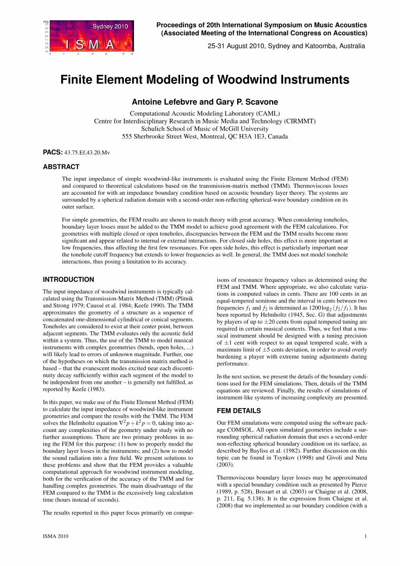
Figure 1: Normalized input impedance of a closed cylinder ofdiameter 15mm and length 300mm: FEM results (filled circles)and theoretical solution (solid line).

with varying boundary conditions at their ends. We were par-ticularly interested in verifying the accuracy of the boundarylayer impedance model and non-reflecting radiation boundarycondition.

A 3D FEM simulation of a closed cylindrical pipe of diame-ter 15mm and length 300mm was first computed. To minimizecomputation time, system symmetries were exploited. The cylin-der was split in two along its primary axis and a null normalacceleration boundary condition was imposed on the plane ofsymmetry. A rigid boundary (v̂n = 0) was created at the pipeend, while the boundary condition along the side walls wasthat given by Eq. 1. The results of the FEM simulation (filledcircles) are shown in Fig. 1 compared to the TMM calculations(solid line). The mesh consists of 2003 cubic elements, giv-ing a total of 12354 degrees of freedom. The first resonancefrequency obtained using the FEM and TMM was 571.74Hzand 571.69Hz, respectively, a difference smaller than 0.2 cents.The ratio of the resonance magnitude is about 0.1 dB. Resultsfor the second resonance were even closer, indicating that theboundary condition for wall losses provides accurate results.

The second validation simulation involved replacing the rigidboundary at the pipe output with the impedance boundary con-dition of Eq. 12, which is the same expression used for theTMM calculations. Discrepancies were again below 0.2 cents.

Next, we simulated the same cylindrical pipe but with the openend radiating into a spherical radiation domain of 50cm radiusand a non-reflecting boundary condition on its outer edge. Theexterior of the pipe was considered rigid (boundary layer losseswere neglected outside the pipe). We found that the refinementof the mesh along the edge at the opening of the pipe influencessignificantly the radiation length correction of the pipe. Wesimulated the same open pipe with an increasing number ofelements on this edge and found that the circumference mustbe approximated with about 300 elements to attain numericalconvergence. Once again, discrepancies were below 0.2 cents.

The same procedure was performed for a conical pipe of length300mm, with an input diameter of 15.0mm and an output diam-eter of 30.7mm (half angle is 1.5 degrees). The discrepanciesbetween the resonance frequencies computed using the FEMand TMM were slightly larger than for the cylindrical geome-try, but they were still below 0.5 cents for the closed cone andthe cone terminated by the radiation impedance. We believethese discrepancies may come from the theoretical model (Ku-lik 2007), which does not take into account the variation of thecomplex characteristic impedance along the cone. This error issufficiently small to be neglected. For the cone radiating into a

Method f1 [Hz] (cents) f2 [Hz] (cents)

Cylinder with one hole closed

FEM 280.68 842.84Dalmont w/o losses 280.80 (0.7) 842.90 (0.1)Dalmont with losses 280.80 (0.7) 842.86 (0.1)Lefebvre w/o losses 280.72 (0.3) 842.90 (0.1)Lefebvre with losses 280.71 (0.1) 842.86 (0.1)

Cylinder with one hole open


Cone with one hole closed


Cone with one hole open

FEM 572.85 1019.35Dalmont w/o losses 573.98 (3.4) 1020.70 (2.3)Dalmont with losses 573.86 (3.1) 1020.55 (2.0)Lefebvre w/o losses 573.57 (2.2) 1019.46 (0.2)Lefebvre with losses 573.30 (1.4) 1019.11 (-0.4)

Table 1: Comparison of the resonance frequencies for the cylin-drical and conical waveguide with one open or closed tonehole.The numbers in parentheses represent the intervals in centsrelative to the FEM result.

sphere, the first resonance was approximately 1 cent lower inthe FEM simulation, indicating that the radiation model of anunflanged pipe may be inadequate when used at the end of aconical waveguide (though the discrepancy is relatively small).

From these validation tests, we conclude that the boundarycondition for the thermoviscous losses and the non-reflectingspherical wave boundary condition can be used successfully forthe simulation of woodwind instruments and that the maximumerror in the calculated resonance frequencies up to 1500Hzusing the TMM is on the order of 1 cent.

WAVEGUIDES WITH A SINGLE TONEHOLE

The input impedance of a cylindrical and a conical waveguidewith a single tonehole was calculated with the FEM and TMM.These geometries allow us to verify the accuracy of the toneholemodels while avoiding possible interactions between adjacentholes. In the FEM, the boundary condition approximating theboundary layer losses is defined on all interior surfaces, includ-ing the tonehole walls. Boundary layer losses are not normallyaccounted for along tonehole walls using the TMM. Thus, dis-crepancies between the FEM and TMM results in this sectionare primarily attributable to these losses and, for the conicalwaveguide, the influence of a main bore taper.

The cylindrical and conical pipes described in the validationsection were modified to include a tonehole of height t = 2mmand δ = b/a = 0.7. For the cylindrical pipe, the tonehole islocated at 87.7mm from the open end, while it is located at141.4mm from the open end of the conical waveguide.

The FEM simulations are in good agreement with TMM calcula-tions for closed side holes. The revised TMM model proposed in

ISMA 2010, associated meeting of ICA 2010 3


Method f1 [Hz] (cents) f2 [Hz] (cents) f3 [Hz] (cents) f4 [Hz] (cents)

Closed toneholes

FEM 143.23 297.43 460.45 630.03Dalmont with losses 144.01 (9.3) 298.39 (5.6) 461.02 (2.1) 630.73 (1.9)Lefebvre with losses 143.45 (2.5) 297.72 (1.7) 460.62 (0.6) 630.00 (-0.1)

Open toneholes

FEM 172.26 364.93 569.13 774.87Dalmont with losses 172.62 (3.6) 365.77 (3.9) 570.81 (5.1) 778.62 (8.4)Lefebvre with losses 172.63 (3.8) 365.73 (3.8) 570.48 (4.1) 777.26 (5.3)

Table 2: Comparison of the simulated and calculated resonance frequencies of a conical waveguide with three open or closed toneholes.

102 103

Frequency (Hz)

10−2

10−1

100

101

102

Zin

102 103

Frequency (Hz)

10−2

10−1

100

101

102

Zin

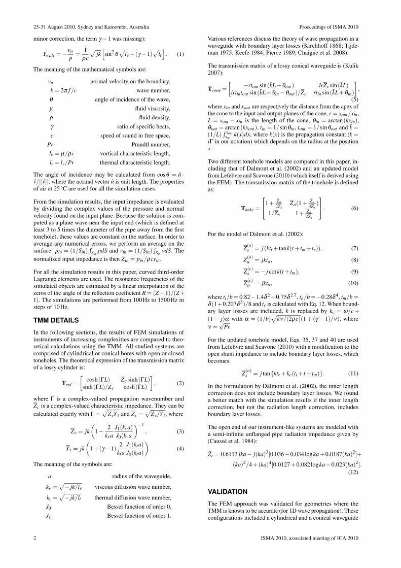
Figure 2: Input impedance of a conical waveguide with threetoneholes: all closed (top graph) and all open (bottom graph).Comparison between the FEM (filled circles) and the TMM(solid). The dashed line is an interpolation between the FEMdata points.

Lefebvre and Scavone (2010) significantly improves the resultsfor toneholes of large diameter and short height. The incorpora-tion of wall losses in the tonehole model does not change theresonances in this case, possibly because these toneholes areshort (t = 2mm). For the conical waveguide, the error of 0.4cents for the first resonance is of the same magnitude as theerror found for the conical waveguide with no toneholes in theprevious section and is therefore not caused by the toneholemodel.

For the open tonehole on a cylindrical bore, the updated TMMtonehole model with boundary layer losses accurately repro-duces the resonance frequencies obtained with the FEM. Theinner length correction needs to include boundary layer lossesas in Eq. 11 to obtain a good match. The effect of the bound-ary layer losses on the tonehole model is expected to be moreimportant for tall toneholes.

There is a discrepancy of 1.4 cents between the FEM and therevised open tonehole TMM model with boundary layer losses

0 200 400 600 800 1000 1200 1400 1600Frequency (Hz)

0.0

0.2

0.4

0.6

0.8

1.0

|Rin|

0 200 400 600 800 1000 1200 1400 1600Frequency (Hz)

0.2

0.3

0.4

0.5

0.6

0.7

0.8

0.9

l o[m

]

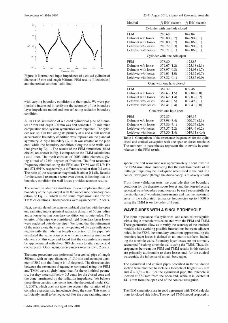
Figure 3: Magnitude of the reflection coefficient (top graph) andopen cylinder equivalent length (bottom graph) for a conicalwaveguide with three open toneholes. Comparison between theFEM (filled circles) and the TMM (solid).

on a conical waveguide. This suggests a potential small effectof the conical waveguide taper on the behaviour of the tonehole.

A CONE WITH THREE TONEHOLES

A conical waveguide of 966.5mm length with an input diameterof 12.5mm and an output diameter of 63.1mm was simulated.Three toneholes, each of 2mm height, were located at distancesof 760mm, 818mm and 879mm from the input plane withrespective diameters of 37.1mm, 39.3mm and 41.6mm. Thesedimensions are close to those of the three toneholes closestto the bell of an alto saxophone. The input impedance of thisinstrument for all toneholes closed and all toneholes open isshown in Fig. 2.

The frequencies of the first four resonances of this system forboth closed and open toneholes are presented in Table 2. Whenall toneholes are closed, the resonance frequencies calculatedusing the TMM with the Lefebvre tonehole model are signifi-cantly closer to those found using the FEM. The discrepanciesbetween these results decrease with increasing frequency andare perhaps caused by internal tonehole interactions.




Closed toneholes

FEM 146.83 439.72 737.72 1032.82Dalmont with losses 146.79 (-0.5) 439.74 (0.1) 737.70 (-0.1) 1032.80 (-0.1)Lefebvre with losses 146.80 (-0.4) 439.78 (0.2) 737.77 (0.1) 1032.92 (0.2)

Open toneholes

FEM 294.55 879.06 1448.49Dalmont with losses 293.44 (-6.6) 879.82 (1.5) 1452.50 (4.8)Lefebvre with losses 293.44 (-6.6) 879.75 (1.3) 1450.66 (2.6)

Table 3: Comparison of the simulated and calculated resonance frequencies of a simple clarinet-like system with twelve open or closedtoneholes.

0 200 400 600 800 1000 1200 1400 1600Frequency (Hz)

10−2

10−1

100

101

102

Zin

200 400 600 800 1000 1200 1400Frequency (Hz)

10−2

10−1

100

101

102

Zin

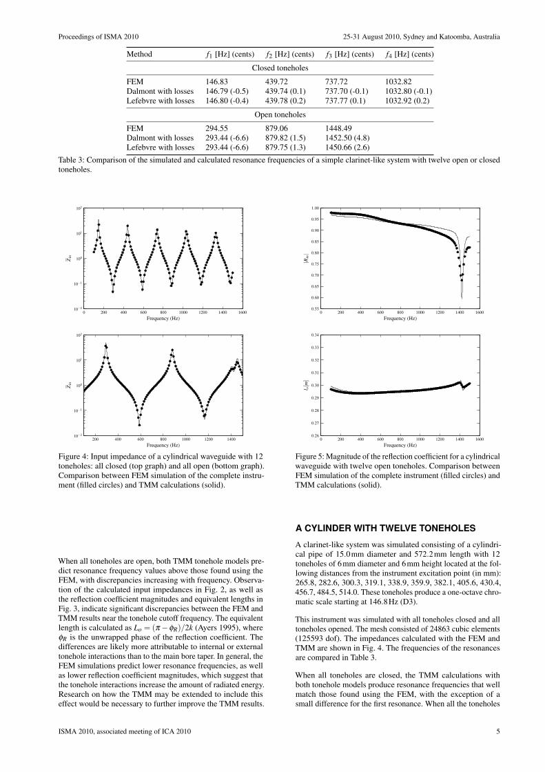
Figure 4: Input impedance of a cylindrical waveguide with 12toneholes: all closed (top graph) and all open (bottom graph).Comparison between FEM simulation of the complete instru-ment (filled circles) and TMM calculations (solid).

When all toneholes are open, both TMM tonehole models pre-dict resonance frequency values above those found using theFEM, with discrepancies increasing with frequency. Observa-tion of the calculated input impedances in Fig. 2, as well asthe reflection coefficient magnitudes and equivalent lengths inFig. 3, indicate significant discrepancies between the FEM andTMM results near the tonehole cutoff frequency. The equivalentlength is calculated as Lo = (π−φR)/2k (Ayers 1995), whereφR is the unwrapped phase of the reflection coefficient. Thedifferences are likely more attributable to internal or externaltonehole interactions than to the main bore taper. In general, theFEM simulations predict lower resonance frequencies, as wellas lower reflection coefficient magnitudes, which suggest thatthe tonehole interactions increase the amount of radiated energy.Research on how the TMM may be extended to include thiseffect would be necessary to further improve the TMM results.

0 200 400 600 800 1000 1200 1400 1600Frequency (Hz)

0.55

0.60

0.65

0.70

0.75

0.80

0.85

0.90

0.95

1.00

|Rin|

0 200 400 600 800 1000 1200 1400 1600Frequency (Hz)

0.26

0.27

0.28

0.29

0.30

0.31

0.32

0.33

0.34

l o[m

]

Figure 5: Magnitude of the reflection coefficient for a cylindricalwaveguide with twelve open toneholes. Comparison betweenFEM simulation of the complete instrument (filled circles) andTMM calculations (solid).

A CYLINDER WITH TWELVE TONEHOLES

A clarinet-like system was simulated consisting of a cylindri-cal pipe of 15.0mm diameter and 572.2mm length with 12toneholes of 6mm diameter and 6mm height located at the fol-lowing distances from the instrument excitation point (in mm):265.8, 282.6, 300.3, 319.1, 338.9, 359.9, 382.1, 405.6, 430.4,456.7, 484.5, 514.0. These toneholes produce a one-octave chro-matic scale starting at 146.8Hz (D3).

This instrument was simulated with all toneholes closed and alltoneholes opened. The mesh consisted of 24863 cubic elements(125593 dof). The impedances calculated with the FEM andTMM are shown in Fig. 4. The frequencies of the resonancesare compared in Table 3.

When all toneholes are closed, the TMM calculations withboth tonehole models produce resonance frequencies that wellmatch those found using the FEM, with the exception of asmall difference for the first resonance. When all the toneholes



102 103

Frequency (Hz)

10−2

10−1

100

101

102Z

in

102 103

Frequency (Hz)

10−2

10−1

100

101

102

Zin

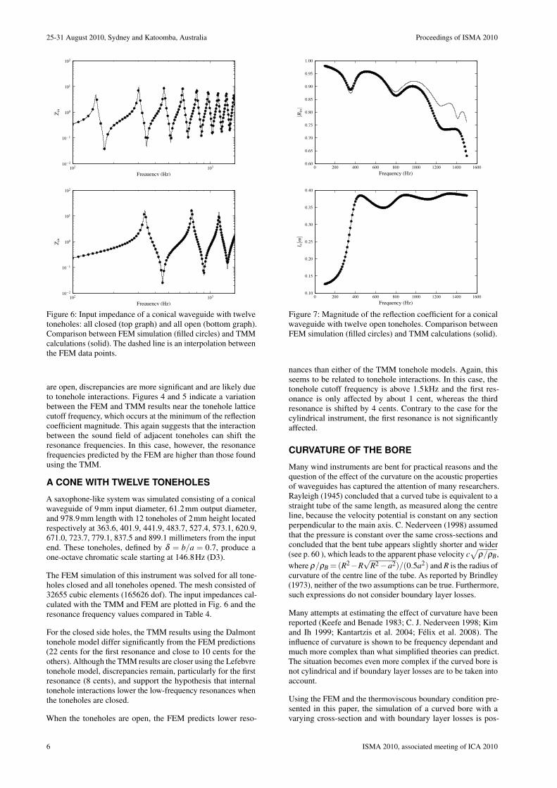
Figure 6: Input impedance of a conical waveguide with twelvetoneholes: all closed (top graph) and all open (bottom graph).Comparison between FEM simulation (filled circles) and TMMcalculations (solid). The dashed line is an interpolation betweenthe FEM data points.

are open, discrepancies are more significant and are likely dueto tonehole interactions. Figures 4 and 5 indicate a variationbetween the FEM and TMM results near the tonehole latticecutoff frequency, which occurs at the minimum of the reflectioncoefficient magnitude. This again suggests that the interactionbetween the sound field of adjacent toneholes can shift theresonance frequencies. In this case, however, the resonancefrequencies predicted by the FEM are higher than those foundusing the TMM.

A CONE WITH TWELVE TONEHOLES

A saxophone-like system was simulated consisting of a conicalwaveguide of 9mm input diameter, 61.2mm output diameter,and 978.9mm length with 12 toneholes of 2mm height locatedrespectively at 363.6, 401.9, 441.9, 483.7, 527.4, 573.1, 620.9,671.0, 723.7, 779.1, 837.5 and 899.1 millimeters from the inputend. These toneholes, defined by δ = b/a = 0.7, produce aone-octave chromatic scale starting at 146.8Hz (D3).

The FEM simulation of this instrument was solved for all tone-holes closed and all toneholes opened. The mesh consisted of32655 cubic elements (165626 dof). The input impedances cal-culated with the TMM and FEM are plotted in Fig. 6 and theresonance frequency values compared in Table 4.

For the closed side holes, the TMM results using the Dalmonttonehole model differ significantly from the FEM predictions(22 cents for the first resonance and close to 10 cents for theothers). Although the TMM results are closer using the Lefebvretonehole model, discrepancies remain, particularly for the firstresonance (8 cents), and support the hypothesis that internaltonehole interactions lower the low-frequency resonances whenthe toneholes are closed.

When the toneholes are open, the FEM predicts lower reso-

0 200 400 600 800 1000 1200 1400 1600Frequency (Hz)

0.60

0.65

0.70

0.75

0.80

0.85

0.90

0.95

1.00

|Rin|

0 200 400 600 800 1000 1200 1400 1600Frequency (Hz)

0.10

0.15

0.20

0.25

0.30

0.35

0.40

l o[m

]

Figure 7: Magnitude of the reflection coefficient for a conicalwaveguide with twelve open toneholes. Comparison betweenFEM simulation (filled circles) and TMM calculations (solid).

nances than either of the TMM tonehole models. Again, thisseems to be related to tonehole interactions. In this case, thetonehole cutoff frequency is above 1.5kHz and the first res-onance is only affected by about 1 cent, whereas the thirdresonance is shifted by 4 cents. Contrary to the case for thecylindrical instrument, the first resonance is not significantlyaffected.

CURVATURE OF THE BORE

Many wind instruments are bent for practical reasons and thequestion of the effect of the curvature on the acoustic propertiesof waveguides has captured the attention of many researchers.Rayleigh (1945) concluded that a curved tube is equivalent to astraight tube of the same length, as measured along the centreline, because the velocity potential is constant on any sectionperpendicular to the main axis. C. Nederveen (1998) assumedthat the pressure is constant over the same cross-sections andconcluded that the bent tube appears slightly shorter and wider(see p. 60 ), which leads to the apparent phase velocity c

√ρ/ρB,

where ρ/ρB =(R2−R√

R2−a2)/(0.5a2) and R is the radius ofcurvature of the centre line of the tube. As reported by Brindley(1973), neither of the two assumptions can be true. Furthermore,such expressions do not consider boundary layer losses.

Many attempts at estimating the effect of curvature have beenreported (Keefe and Benade 1983; C. J. Nederveen 1998; Kimand Ih 1999; Kantartzis et al. 2004; Félix et al. 2008). Theinfluence of curvature is shown to be frequency dependant andmuch more complex than what simplified theories can predict.The situation becomes even more complex if the curved bore isnot cylindrical and if boundary layer losses are to be taken intoaccount.

Using the FEM and the thermoviscous boundary condition pre-sented in this paper, the simulation of a curved bore with avarying cross-section and with boundary layer losses is pos-




Closed toneholes

FEM 147.19 302.58 461.63 628.60Dalmont with losses 149.06 (21.9) 304.10 (8.7) 463.98 (8.8) 631.94 (9.2)Lefebvre with losses 147.85 (7.8) 302.63 (0.3) 461.97 (1.3) 628.76 (0.2)

Open toneholes

FEM 334.14 733.03 1154.32Dalmont with losses 334.31 (0.8) 734.35 (3.1) 1158.30 (6.0)Lefebvre with losses 334.28 (0.7) 734.06 (2.4) 1156.56 (3.4)

Table 4: Comparison of the simulated and calculated resonance frequencies of a conical waveguide with twelve open or closed toneholes.

Method f1 [Hz] (cents) f2 [Hz] (cents) f3 [Hz] (cents) f4 [Hz] (cents) f5 [Hz] (cents)

straight (1) 145.03 304.92 473.41 640.97 804.22curved (2) 145.04 (0.1) 304.97 (0.2) 473.58 (0.6) 641.30 (0.9) 804.57 (0.8)curved (3) 145.05 (0.2) 305.09 (0.9) 473.98 (2.1) 642.07 (3.0) 805.39 (2.5)

straight (TMM) 144.90 (-1.6) 305.24 (1.8) 473.68 (1.0) 640.95 (0.0) 804.19 (-0.1)

Table 5: Comparison of the simulated and calculated resonance frequencies of a conical waveguide with twelve open or closed toneholes.

24

23

15.5 12.5 12.5

76 70 30

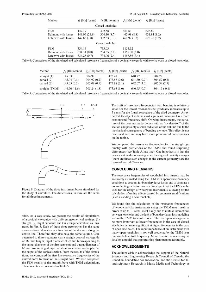
Figure 8: Diagram of the three instrument bores simulated forthe study of curvature. The dimensions, in mm, are the samefor all three instruments.

sible. As a case study, we present the results of simulationsof a conical waveguide with different geometrical settings: (1)straight, (2) slight curvature and (3) stronger curvature, as illus-trated in Fig. 8. Each of these three geometries has the samecross-sectional diameter as a function of the distance along thecentre line. Therefore, they also have the same volume. Con-catenated to these segments was a straight conical waveguideof 760mm length, input diameter of 23mm (corresponding tothe output diameter of the first segment) and output diameter of63mm. An unflanged pipe radiation impedance was applied atthe output of the conical section. From the results of the simula-tions, we compared the first five resonance frequencies of thecurved bores to those of the straight bore. We also comparedthe FEM results of the straight bore with TMM calculations.These results are presented in Table 5.

The shift of resonance frequencies with bending is relativelysmall for the lowest resonances but gradually increases up to3 cents for the fourth resonance of the third geometry. As ex-pected, the object with the most significant curvature has a morepronounced frequency shift. On wind instruments, the curva-ture of the bore normally comes with an “ovalisation” of thesection and possibly a small reduction of the volume due to themechanical consequence of bending the tube. This effect is notdiscussed here and may have more pronounced consequenceson the tuning.

We compared the resonance frequencies for the straight ge-ometry with predictions of the TMM and found surprisingdifferences (see Table 5, last line). One hypothesis is that theevanescent modes occurring when the angle of conicity changes(there are three such changes in the current geometry) are thecause of such differences.

CONCLUDING REMARKS

The resonance frequencies of woodwind instruments may beaccurately estimated using the FEM with appropriate boundaryconditions to account for boundary layer losses and to simulate anon-reflecting radiation domain. We expect that the FEM can beused for the design of woodwind instruments, allowing for thecalculation of tuning effects caused by geometry modifications(such as adding a new tonehole).

We found that the calculation of the resonance frequenciesof woodwind-like instruments using the TMM may result inerrors of up to 10 cents, most likely due to mutual interactionsbetween toneholes and the lack of boundary layer loss modelingwithin the TMM tonehole model. The discrepancies appear tobe more important at lower frequencies in the case of closedside holes but more significant at higher frequencies in the caseof open side holes. The input impedance of an instrument withmany open toneholes is not well predicted by the TMM nearthe tonehole cutoff frequency. More research is necessary todevelop a model that captures this phenomenon accurately.

ACKNOWLEDGMENTS

The authors wish to acknowledge the support of the NaturalSciences and Engineering Research Council of Canada, theCanadian Foundation for Innovation, and the Centre for In-terdisciplinary Research in Music Media and Technology at



McGill University. The first author gratefully acknowledges theFonds Québécois de la Recherche sur la Nature et les Technolo-gies for a doctoral research scholarship.

REFERENCES

Ayers, R. Dean (1995). “Two complex effective lengths formusical wind instruments”. J. Acoust. Soc. Am. 98, pp. 81–87.

Bayliss, Alvin et al. (1982). “Boundary Conditions for the Nu-merical Solution of Elliptic Equations in Exterior Regions”.SIAM Journal on Applied Mathematics 42, pp. 430–451.

Bossart, R. et al. (2003). “Hybrid numerical and analyticalsolutions for acoustic boundary problems in thermo-viscousfluids”. J. Sound Vibrat. 263, pp. 69–84.

Brindley, G. S. (1973). “Speed of Sound in Bent Tubes and theDesign of Wind Instruments”. Nature 246, pp. 479–480.

Caussé, René et al. (1984). “Input impedance of brass musi-cal instruments – Comparison between experimental andnumerical models”. J. Acoust. Soc. Am. 75, pp. 241–254.

Chaigne, Antoine et al. (2008). Acoustique des instruments demusique. Paris, France: Éditions Belin.

Dalmont, Jean-Pierre et al. (2002). “Experimental Determina-tion of the Equivalent Circuit of an Open Side Hole: Linearand Non Linear Behaviour”. Acustica 88, pp. 567–575.

Félix, Simon et al. (2008). “Effect of bending portions of the aircolumn on the acoustical properties of a wind instrument”.J. Acoust. Soc. Am. 123, p. 3447.

Givoli, Dan and Beny Neta (2003). “High-order non-reflectingboundary scheme for time-dependent waves”. Journal ofComputational Physics 186, pp. 24–46.

Helmholtz, Hermann von (1945). On the sensation of tone.Dover Publications.

Kantartzis, Nikolaos V. et al. (2004). “A 3D multimodal FDTDalgorithm for electromagnetic and acoustic propagationin curved waveguides and bent ducts of varying cross”.COMPEL 23, pp. 613–624.

Keefe, Douglas H. (1983). “Acoustic streaming, dimensionalanalysis of nonlinearities, and tone hole mutual interactionsin woodwinds”. J. Acoust. Soc. Am. 73, pp. 1804–1820.

— (1984). “Acoustical wave propagation in cylindrical ducts:Transmission line parameter approximations for isothermaland nonisothermal boundary conditions”. J. Acoust. Soc.Am. 75, pp. 58–62.

— (1990). “Woodwind air column models”. J. Acoust. Soc.Am. 88, pp. 35–51.

Keefe, Douglas H. and Arthur H. Benade (1983). “Wave prop-agation in strongly curved ducts”. J. Acoust. Soc. Am. 74,pp. 320–332.

Kim, Jun-Tai and Jeong-Guon Ih (1999). “Transfer matrix ofcurved duct bends and sound attenuation in curved expan-sion chambers”. Appl. Acoust. 56, pp. 297–309.

Kirchhoff, G. (1868). “On the Influence of Heat Conductionin a Gas on Sound Propagation”. Ann. Phys. Chem. 134,pp. 177–193.

Kulik, Yakov (2007). “Transfer matrix of conical waveguideswith any geometric parameters for increased precision incomputer modeling”. J. Acoust. Soc. Am. 122, EL179–EL184.

Lefebvre, Antoine and Gary P. Scavone (2010). “Refinementsto the Model of a Single Woodwind Instrument Tonehole”.Proceedings of the 2010 International Symposium on Musi-cal Acoustics. Sydney and Katoomba, Australia.

Nederveen, Cornelis Johannes (1998). Acoustical Aspects ofWoodwind Instruments. Revised. DeKalb, Illinois: NorthernIllinois University Press, p. 147.

Nederveen, Cornelis Johannes (1998). “Influence of a toroidalbend on wind instrument tuning”. J. Acoust. Soc. Am. 104,pp. 1616–1626.

Pierce, Allan D. (1989). Acoustics, An Introduction to Its Phys-ical Principles and Applications. Woodbury, New-York:Acoustical Society of America, p. 678.

Plitnik, George R. and William J. Strong (1979). “Numericalmethod for calculating input impedances of the oboe”. J.Acoust. Soc. Am. 65, pp. 816–825.

Rayleigh, J.W.S. (1945). The Theory of Sound. Vol. 2. NewYork: Dover Publications.

Tijdeman, H. (1975). “On the propagation of sound waves incylindrical tubes”. J. Sound Vibrat. 39, pp. 1–33.

Tsynkov, S. V. (1998). “Numerical solution of problems onunbounded domains. A review”. Applied Numerical Mathe-matics 27, pp. 465–532.


finite element modeling of woodwind instruments

Documents