fingerprint matching using small sensors
TRANSCRIPT
Faculty of engineering, LTH
Centre for mathematical sciences
Master Thesis
Fingerprint Matching using SmallSensors
Rikard [email protected]
Supervisor
Magnus Oskarsson
Examiner
Anders Heyden
April 2017

Abstract
Fingerprint software is widely used in applications such as smartphones. There has tobe some overlap between two fingerprint samples in order for them to be considered asbelonging to the same finger. Determining if this overlap exists is normally not a problemif a fingerprint sensor is big enough to capture a sample from the whole finger at once.However, if the sensor is small it might capture samples from different parts of the samefinger such that there is no overlap. To find a predictor one needs a training set butconstructing the set using small sensors lead to a highly noisy set. This project examinessome methods to filter the noise. None of the filtering methods provided a conclusiveimprovement on all datasets compared to the already implemented method. The mostpromising methods, however, includes a substitution of the SVM algorithm with S3VMand either to use no filtering, random downsampling of the majority class or a recursivefilter.
Keywords. Fingerprint, small sensor, noise, filter, SVM, S3VM , SMOTE, ADASYN.

Acknowledgements
I would like to thank the R&D team at Precise Biometrics for providing the foundationfor an interesting project. Special thanks to Karl Netzell for exceptional guidance andinsightful comments. Thanks also to Rutger Petersson for taking me on board and toMagnus Oskarsson for supervising the project.
Contents
1 Introduction 41.1 Fingerprint systems . . . . . . . . . . . . . . . . . . . . . . . . . . . . . . 51.2 Fingerprint characteristics . . . . . . . . . . . . . . . . . . . . . . . . . . 71.3 Template matching . . . . . . . . . . . . . . . . . . . . . . . . . . . . . . 71.4 System errors . . . . . . . . . . . . . . . . . . . . . . . . . . . . . . . . . 91.5 A brief introduction to machine learning . . . . . . . . . . . . . . . . . . 101.6 Problem formulation . . . . . . . . . . . . . . . . . . . . . . . . . . . . . 10
2 Theory 122.1 The matching module . . . . . . . . . . . . . . . . . . . . . . . . . . . . 122.2 Matching module errors . . . . . . . . . . . . . . . . . . . . . . . . . . . 132.3 Machine learning . . . . . . . . . . . . . . . . . . . . . . . . . . . . . . . 15
2.3.1 Predictor errors . . . . . . . . . . . . . . . . . . . . . . . . . . . . 162.3.2 Overfitting . . . . . . . . . . . . . . . . . . . . . . . . . . . . . . . 162.3.3 Crossvalidation . . . . . . . . . . . . . . . . . . . . . . . . . . . . 17
2.4 Algorithms . . . . . . . . . . . . . . . . . . . . . . . . . . . . . . . . . . . 182.4.1 Linear predictors . . . . . . . . . . . . . . . . . . . . . . . . . . . 182.4.2 Support Vector Machine (SVM) . . . . . . . . . . . . . . . . . . . 192.4.3 Semi-Supervised Support Vector Machine (S3VM) . . . . . . . . . 202.4.4 Parameter selection . . . . . . . . . . . . . . . . . . . . . . . . . . 22
2.5 Dataset characteristics . . . . . . . . . . . . . . . . . . . . . . . . . . . . 232.5.1 Noise . . . . . . . . . . . . . . . . . . . . . . . . . . . . . . . . . . 23
3 Datasets and tools 243.1 The dataset structure . . . . . . . . . . . . . . . . . . . . . . . . . . . . . 243.2 The datasets . . . . . . . . . . . . . . . . . . . . . . . . . . . . . . . . . . 25
3.2.1 Dataset SA . . . . . . . . . . . . . . . . . . . . . . . . . . . . . . 253.2.2 Dataset SB . . . . . . . . . . . . . . . . . . . . . . . . . . . . . . 253.2.3 Dataset SC . . . . . . . . . . . . . . . . . . . . . . . . . . . . . . 253.2.4 Match information . . . . . . . . . . . . . . . . . . . . . . . . . . 263.2.5 Memory limitations . . . . . . . . . . . . . . . . . . . . . . . . . . 26
3.3 Tools . . . . . . . . . . . . . . . . . . . . . . . . . . . . . . . . . . . . . . 273.3.1 Matlab/Octave . . . . . . . . . . . . . . . . . . . . . . . . . . . . 273.3.2 LIBLINEAR . . . . . . . . . . . . . . . . . . . . . . . . . . . . . . 273.3.3 SVMLIN . . . . . . . . . . . . . . . . . . . . . . . . . . . . . . . . 283.3.4 FLANN . . . . . . . . . . . . . . . . . . . . . . . . . . . . . . . . 28
1

CONTENTS 2
4 The original algorithm 294.1 Introduction . . . . . . . . . . . . . . . . . . . . . . . . . . . . . . . . . . 294.2 The training algorithm AP . . . . . . . . . . . . . . . . . . . . . . . . . . 30
4.2.1 The inner training algorithm AP . . . . . . . . . . . . . . . . . . 31
5 The new algorithm 335.1 Introduction . . . . . . . . . . . . . . . . . . . . . . . . . . . . . . . . . . 335.2 The training algorithm AN . . . . . . . . . . . . . . . . . . . . . . . . . . 33
5.2.1 The inner training algorithm AN . . . . . . . . . . . . . . . . . . 345.3 The selection function µN . . . . . . . . . . . . . . . . . . . . . . . . . . 345.4 The filter functions ρ . . . . . . . . . . . . . . . . . . . . . . . . . . . . . 34
5.4.1 ADASYN . . . . . . . . . . . . . . . . . . . . . . . . . . . . . . . 355.4.2 SMOTE . . . . . . . . . . . . . . . . . . . . . . . . . . . . . . . . 375.4.3 Grey data . . . . . . . . . . . . . . . . . . . . . . . . . . . . . . . 375.4.4 Mark below . . . . . . . . . . . . . . . . . . . . . . . . . . . . . . 375.4.5 Random downsampling . . . . . . . . . . . . . . . . . . . . . . . . 385.4.6 Recursive . . . . . . . . . . . . . . . . . . . . . . . . . . . . . . . 385.4.7 Voting filter . . . . . . . . . . . . . . . . . . . . . . . . . . . . . . 38
5.5 Feature transformation . . . . . . . . . . . . . . . . . . . . . . . . . . . . 40
6 Results 426.1 Evaluation procedure . . . . . . . . . . . . . . . . . . . . . . . . . . . . . 42
6.1.1 The baseline . . . . . . . . . . . . . . . . . . . . . . . . . . . . . . 436.1.2 Parameters for the ρ and µN functions . . . . . . . . . . . . . . . 436.1.3 Initial subset . . . . . . . . . . . . . . . . . . . . . . . . . . . . . 44
6.2 Algorithmic performance using β0N = βP . . . . . . . . . . . . . . . . . . 44
6.3 Algorithmic performance using β0N = βR . . . . . . . . . . . . . . . . . . 46
6.3.1 Convergence . . . . . . . . . . . . . . . . . . . . . . . . . . . . . . 466.4 Overfitting . . . . . . . . . . . . . . . . . . . . . . . . . . . . . . . . . . . 476.5 Feature transform - Centroid method . . . . . . . . . . . . . . . . . . . . 48
7 Conclusions 497.1 Future work . . . . . . . . . . . . . . . . . . . . . . . . . . . . . . . . . . 49
7.1.1 Feature transformation . . . . . . . . . . . . . . . . . . . . . . . . 497.1.2 Robust SVM . . . . . . . . . . . . . . . . . . . . . . . . . . . . . 50
8 Appendix 518.1 The original training structure . . . . . . . . . . . . . . . . . . . . . . . . 51
8.1.1 Functions . . . . . . . . . . . . . . . . . . . . . . . . . . . . . . . 518.2 The new training structure . . . . . . . . . . . . . . . . . . . . . . . . . . 53
8.2.1 Functions . . . . . . . . . . . . . . . . . . . . . . . . . . . . . . . 538.2.2 An example . . . . . . . . . . . . . . . . . . . . . . . . . . . . . . 55

CONTENTS 3
Symbols, terms and functions
Table 1 contains a summary of the symbols, terms and functions that are used in thisreport.
Symbol/Term/Function MeaningR The set of real numbers.Rn The set of n-dimensional vectors over R.N The set of natural numbers.T Enrollment template.I Verification template.F Feature vector.T Multitemplate.I Set of verification templates.F Multifeature.X Domain set.Y Label set.LD,f True error.AL(S) Linear training algorithm SVM or S3VM working on dataset S.AP (S) Original training algorithm working on dataset S.AN(S) New training algorithm working on dataset S.λP Predictor returned by the original training algorithm AP (S)λN Predictor returned by the new training algorithm AP (S)α Feature function.β Score function.γ Decision function.FAR False Accept Rate.FRR False Reject Rate.Sample Digital representation of a part or a full fingerprint.Template Compact representation of sample.Multitemplate Collection of templates.Genuine match Match between two templates from the same finger.Impostor match Match between two templates from two different fingers.
Table 1: Symbols, terms and functions.

Chapter 1
Introduction
Biometric recognition refers to the use of distinctive anatomical and behavioral char-acteristics, called biometric identifiers, for recognizing individuals [1, p.2]. Examples ofanatomical characteristics are fingerprints, irises and facial features. Speech is an exampleof a behavioral characteristic. This method of recognition has garnered interest duringthe last century since biometric identifiers cannot be shared or misplaced. Fingerprintsare among the more popular biometric identifiers [1, p.12]. In 1893, the Home MinistryOffice, UK, accepted that no two individuals have the same fingerprints [1, p.2]. Sincethen, fingerprints have been used extensively in crime investigations. Early fingerprintanalysis used a manual method of visual comparison which was tedious and slow. Morerecently, with the help of computers, the process has been able to become automated. Be-cause of this, fingerprint technology has been integrated into devices such as smartphonesand tablets to provide a method for easy system access.
Precise Biometrics AB provides fingerprint software and smart card readers for digitalauthentication of identity. Their fingerprint algorithm solution has been integrated intohundreds of millions of mobile phones and tablets worldwide. It is well suited for productswith limited processing power and memory such as payment cards, wearables, accesscontrol systems, the Internet of Things and products with small sensors. Since the adventof devices such as smartphones where space is a valuable commodity, it has been of interestto shrink the size of the fingerprint sensors [1, p.89]. However, the smaller sensor sizemakes it harder to accurately perform fingerprint recognition. Precise Biometrics hasdeveloped high performing algorithm solutions specifically for use with small sensors.There is nevertheless room for improvement. This project evaluates different methodsaimed at improving these algorithms.
This report is divided into eight chapters. Chapter 1 contains an overview of concepts ofimportance to fingerprint systems. Chapter 2 then provides a more in depth look at someof these concepts. An introduction to the datasets and tools used in this project is foundin chapter 3. How the concepts, datasets and tools are connected in Precise Biometrics’current system is explored in chapter 4. Chapter 5 contains the details of the changesmade to the system during this project. The effects of these changes and some commentsare found in chapter 6 and 7. Chapter 8 provides information about the implementationsof the functions in chapter 4 and 5.
4

CHAPTER 1. INTRODUCTION 5
1.1 Fingerprint systems
A fingerprint system may be a verification system or an identification system [1, p.3]. Averification system authenticates the claimed identity of a person by comparing a capturedfingerprint with a previously captured template containing fingerprint data connected tothe claimed identity. The output of a verification system is an accept or reject decisionindicating whether the system believes that the person is who he/she claims to be.
With an identification system, the person makes no prior identity claim. Instead theentire template database is searched for a match. The output in this case is the identityconnected to a template that matched sufficiently well. The output may be empty ifno template matched well enough. An identification system can be implemented byletting a verification system perform a one-to-many comparison against an entire templatedatabase. The focus in this project is on the verification system.
Two processes are shown in figure 1.1: enrollment and verification. The enrollmentprocess registers the fingerprint information from individuals and saves it in the systemstorage. The verification process is responsible for confirming the claim of identity ofthe subject. The claim can be made with the help of a user name, a PIN number orthrough information stored on a proximity card, depending on the type of system. Asseen in figure 1.1, the enrollment and the verification processes can be broken down intothe following modules:
• Capture: a digital representation of a fingerprint is captured using a sensor. Thecaptured representation is known as a sample.
• Template creation: the sample is processed to extract the essential informationcontained in the fingerprint. This creates a more compact representation of thesample, known as a template. Using the template instead of the raw sample isoften beneficial in terms of storage space and system speed.
• Matching : the matching module decides whether two templates should be consid-ered as belonging to the same finger. This module can be broken down into threesub-modules. The first sub-module takes a verification template (obtained from anew sample) and an enrollment template (from the system storage) as inputs andproduces a feature set containing information about the similarity of the two tem-plates. This feature set is used as input to the second sub-module which calculatesa similarity score. The similarity score is then compared to a predefined systemthreshold in the third sub-module. The templates are deemed to represent the samefinger only if the similarity score is above the system threshold. If this is the case,the matching module makes a match (or accept) decision. If the score is below thethreshold, the decision is non-match (or reject).

CHAPTER 1. INTRODUCTION 6
Sample Template
Template identifier
Enrollment process
Datastorage
Templatecreation
Capture
Sample Template
Claimed identity
Verification process
Datastorage
Templatecreation
Capture Matching Template
Match or non-match
Figure 1.1: Overview of the enrollment and verification processes. The enrollment process isresponsible for creating and storing the enrollment template that has been extracted from acaptured sample. In the verification process, a new sample is captured and converted intoa verification template. This template is then compared to a previously stored enrollmenttemplate and a match/accept or non-match/reject decision is made depending on the similarityof the two templates and the system threshold.

CHAPTER 1. INTRODUCTION 7
1.2 Fingerprint characteristics
The fingerprint system in section 1.1 and figure 1.1 utilizes a module called templatecreation which extracts the essential information from a captured sample. This sectionexplores the kind of information that may be extracted during this stage.
A fingerprint is the reproduction of the exterior appearance of the fingertip epidermis(the outer of the two layers that make up the skin). Figure 1.2 shows some of themost characteristic features of a fingerprint, ridges and valleys [1, p.97]. The ridges arethe dark lines and the valleys are the bright lines. A fingerprint consists of a series ofinterleaved ridges and valleys. It is common to describe ridge characteristics with threelevels of detail. Level 1 is the overall global ridge flow pattern. Level 2 (local level) arethe minutiae (small detail) points. Among Level 3 are things like pores and the localshape of ridge edges.
The global patterns in Level 1 can be classified into three categories, loops, deltas andwhorls [1, p.98]. Examples of these can be seen in figure 1.3. Compared to the otherareas of the fingerprint which consist of mainly parallel ridges, these areas contain highercurvature and frequent ridge terminations. The loop, delta and whorl types are typicallycharacterized by ∩, ∆ and O shapes respectively.
Minutiae are part of the local level (Level 2) characteristics [1, p.99]. Examples of minu-tiae are ridges that come to an end or divide into two ridges as can be seen in figure 1.4.These are called ridge endings and bifurcations respectively. Minutiae are the most com-monly used characteristics in automatic fingerprint matching and it has been observedthat minutiae do not change during an individual’s lifetime.
Level 3 contains the very local characteristics [1, p.101]. These include the width, shapeand edge contour of the ridges. The ridges are dotted with sweat pores which can alsobe used to identify a person assuming a sufficiently high resolution fingerprint sensor isused.
In order for the characteristics to be used in an automatic system they have to be quanti-fied in some way. A ridge ending minutia may for example be quantified using three num-bers; the two planar coordinates and the directional angle of the ridge ending tip.
1.3 Template matching
The matching module compares two templates and returns a decision on whether theymatch or not. The output of the first sub-module in the matching module is a feature set.This feature set is produced by comparing the two input templates. A template is simplyput a collection of numbers (called descriptors) that are quantifications of the fingerprintcharacteristics as seen in section 1.2. A possible method for measuring the similarity oftwo templates is to measure the distance between their descriptors using some norm, e.g.the Euclidean or Hamming norm.

CHAPTER 1. INTRODUCTION 8
Figure 1.2: Example of a fingerprint sample. The dark lines are the ridges. The white spaceinbetween the ridges are the valleys.
Figure 1.3: Examples of loops (∩), deltas (∆) and whorls and (O) in fingerprints.
Figure 1.4: A ridge ending and a bifurcation.

CHAPTER 1. INTRODUCTION 9
Figure 1.5: The overlap between the enrollment template (red) and the verification template(green) is non-existent due to a small sensor.
1.4 System errors
There are many reasons why the fingerprint system could make the wrong decision andallow or deny access to the wrong person [1, p.12-14]. Problems with the sensor couldlead to errors of the types: Failure to Detect (FTD) and Failure to Capture (FTC), whichrespectively refer to the sensor failing to detect the presence of a finger and failure tocapture a sample of sufficient quality. Failure to Process (FTP) occurs when the templateextraction module is unable to extract a usable template from the sample.
An information limitation error occurs for example when a verification template andan enrollment template are from different parts of the same finger and there is verylittle overlap between the two [1, p.12]. This situation is common if the sensor size issmall and unable to capture a full fingerprint in one sample. Figure 1.5 illustrates thisproblem. Even though both the enrollment and the verification template come fromthe same finger it is very likely that the owner of this fingerprint would be rejecteddue to the lack of similarity between the two templates. To increase the possibilityof overlap between the enrollment and verification template, a method which is usedby Precise Biometrics is to let users provide a set of enrollment templates, known asa multitemplate (figure 1.6), from each finger during the enrollment phase. With thismethod, a finger is accepted if the verification template is sufficiently similar to any ofthe templates in a multitemplate. Naturally, provided that the sensor is small enoughand that the templates in the multitemplate are evenly distributed over the finger, averification template is going to lack similarity to many, if not most, of the templatesin the multitemplate. This is true regardless of whether or not the verification templateand the multitemplate are created from the same finger.

CHAPTER 1. INTRODUCTION 10
Figure 1.6: A multitemplate is a collection of enrollment templates (red). The verificationtemplate (green) overlaps only some of the templates in the multitemplate.
1.5 A brief introduction to machine learning
Precise Biometrics utilizes machine learning in the second and third sub-module of thematching module to support its accept or reject decisions. In [2, p.vii, p.19] the subjectof machine learning is introduced as a method of programming computers to learn usingexamples. The goal is to find meaningful, exploitable patterns among a set of examples.Machine learning algorithms may be divided into three different groups; supervised, semi-supervised and unsupervised [2, p.23]. The names of the three groups are connected tothe type of example sets that the different types of algorithms expect as input whenlearning. Supervised learning algorithms expect the data in the training set to be pairedwith a label that indicates what class the example belongs to. Unsupervised learningdoes not expect the data to be labeled. Semi supervised learning is a mixture of thesupervised and unsupervised learning; the dataset can consist of a mixture of labeled andunlabeled data.
1.6 Problem formulation
It is time to formulate the problem that is investigated in this project. The focus is onthe matching module. The second and third sub-module in the matching stage (section1.1) uses machine learning to learn when to make an accept or reject decision. Section1.5 described machine learning as a method for learning from a set of examples. In thisproject, an example is a feature set (section 1.1). The example is connected to a labelindicating whether the feature set is produced by two templates from the same finger ornot. Section 1.4 however mentioned that, when a small sensor is involved, a verificationtemplate is often going to lack similarity to many of the templates in a multitemplateregardless of whether they come from the same finger or not. This means that the example

CHAPTER 1. INTRODUCTION 11
set is going to suffer from noise. The problem that is investigated in this project can beformulated as follows: Is there a better method to remove noise from the example setcompared to the one currently in use by Precise Biometrics?

Chapter 2
Theory
This chapter explores some concepts of importance to the matching module which wasintroduced in section 1.1. However, the details of the actual implementation of thismodule is located in subsequent chapters. Section 2.1 introduces some notation andfunctions that are useful for further discussion of the matching module. Details on howto quantify the performance of the matching module is found in section 2.2. Section 2.3contains a formal introduction to machine learning and some of the common concepts andissues encountered when dealing with this subject. A main concept is the predictor. Sometraining algorithms for linear predictors are explored in section 2.4. These algorithmsrequire a training dataset. Section 2.5 presents some common problems encounteredwhen constructing a training set.
2.1 The matching module
The matching module was introduced in section 1.1 and its place in the overall finger-print system can be seen in figure 1.1. This section contains further details about thismodule.
A template can be regarded as a vector in Rm containing a quantification of the character-istics of a fingerprint sample. Examples of these characteristics were presented in section1.2. The input to the matching module is an enrollment template, T, and a verificationtemplate, I. The output is a binary decision on whether these two templates should beconsidered as belonging to the same finger or not. It was further specified in section 1.1that the matching module consists of three sub-modules. The first sub-module is thefeature function, α : Rm × Rm → Rn. A feature vector is acquired using α(T, I). Thisfeature vector contains information about the similarity of T and I and is the input tothe second sub-module.
The score function is β : Rn → R. A similarity score for a feature vector F can becalculated using β(F). As the name implies, this function calculates a single numberthat measures the similarity of two templates (the dependency of β on the two templates
12

CHAPTER 2. THEORY 13
is implicit in F). Finally, the decision function is γ : R → {0, 1}. A decision is acquiredfrom a similarity score S using γ(S).
The function s(T, I) is used in section 2.2 when discussing error measurements. Thisfunction produces a similarity score from two templates and can be defined as a compositefunction, s := β ◦ α : Rm × Rm → R.
The complete matching module function, m, is acquired by also including the γ functionafter the similarity score calculation, m := γ ◦ β ◦ α : Rm × Rm → {0, 1}. This functiontakes two templates and makes an accept or reject decision.
Finally, a function that is going to be of importance during the remainder of this projectand should be kept in mind especially when reading section 2.3 is the composition ofthe similarity function and the decision function, λ := γ ◦ β : Rn → {0, 1}. This func-tion makes a decision given a feature vector containing similarity measurements of twotemplates.
2.2 Matching module errors
The similarity score that is used in the second sub-module in the matching module canwithout loss of generality be assumed to lie in the interval [0, 1]. The closer a score isto 1, the more certain is the system that the verification template and the enrollmenttemplate comes from the same finger. A decision that the two templates do indeed comefrom the same finger is called a match. The opposite decision is called a non-match. Twotypes of errors can be committed at this stage, the false match and the false non-match.The false match error occurs when the system deems templates from two different fingersto be from the same finger. The false non-match error occurs when templates from onefinger are mistaken for being from two different fingers. False match and false non-matchare often referred to as false acceptance and false rejection. These terms are commonlyused in the commercial sector and are also used in this report. It is also common to usethe false acceptance rate (FAR) and false rejection rate (FRR), as described in detailbelow, when doing performance evaluation of a fingerprint system.
With T and I as in section 2.1, the null and alternate hypothesis are [1, p.16]:
H0: I 6= T, verification template does not come from the same finger as the enrollmenttemplate.
H1: I = T, verification template comes from the same finger as the enrollment template.
The associated decisions are as follows.
D0 : non-acceptance.
D1: acceptance.
Before the final decision in the matching module, the similarity score s(T, I) is produced.By collecting scores from many different template comparisons, both from comparisonsfrom the same finger and from different fingers, one can estimate the score distribution

CHAPTER 2. THEORY 14
p(s). The genuine distribution is a conditional distribution p(s|H1) of scores generatedfrom template comparisons from the same finger. The impostor distribution p(s|H0) isthe score distribution given comparisons from different fingers. If the similarity score isless than a system threshold, t, then D0 is decided, else D1. The FRR and FAR can nowbe declared as
FRR = P (D0|H1) =∫ t0p(s|H1)ds
FAR = P (D1|H0) =∫ 1
tp(s|H0)ds
The FAR and FRR are functions of the system threshold t. By changing the threshold,the FAR and FRR also changes. From figure 2.1 it is apparent that to decrease the FARone can simply increase the threshold. This however has the unfortunate effect of alsoincreasing the FRR. If one wants to decrease the FRR however, the FAR increases. De-pending on where a system is to be deployed, a low FAR level can be more important thana low FRR. In that case it would be beneficial to choose a high system threshold.
By varying the system threshold, new pairs of FAR and FRR can be acquired. Plottingeach pair in a DET graph (Detection Error Tradeoff) is a convenient method of evaluatingand comparing the performance of different systems. Figure 2.2 shows examples of DETcurves for different systems. Since both the FAR and FRR ideally should be a smallas possible for a good system, a curve that is as close as possible to the bottom ispreferred.
Figure 2.1: The FAR and FRR for a given threshold. By moving the threshold it is possible todecrease the FAR at the expense of increasing the FRR and vice versa.

CHAPTER 2. THEORY 15
Figure 2.2: DET curves for different systems. A system with a DET curve close to the bottomis preferred. Here, the red curve indicates the worst performing system.
2.3 Machine learning
This section expands on section 1.5 with a formal introduction to machine learning.
The output of the learning or training process is a prediction rule or predictor [2, p.34].A predictor is used to assign a label to an object. The domain set, X , is the set ofobjects that can be labeled. In this project X = Rn. The label set, Y , is the set oflabels that can be assigned to the objects in X . For binary classification the label set isusually {0, 1} or {−1, 1}. A predictor is a mapping from the domain set to the label set,h : X → Y . The training set, S = {(x1, y1)...(xN , yN)}, is a finite set of pairs in X × Y .A(S) denotes the predictor that is returned by algorithm A using training set S. Theperfect predictor f : X → Y labels all points in the domain set correctly, i.e yi = f(xi)for all i. It is assumed that objects in X are distributed according to some distribution Dsuch that given a subset C ⊂ X , the probability distribution D assigns a number D(C)which determines how likely it is to observe a point x ∈ C. A general dataset, S, canbe thought of as being generated by sampling xi according to the distribution D andassigning a label with yi = f(xi).
The true error of a predictor, h, is LD,f (h) := D({x : h(x) 6= f(x)}) i.e. the probabilityof randomly choosing an example x for which h(x) 6= f(x). The distribution D andthe perfect predictor, f , are unknown during the training process. These are what the

CHAPTER 2. THEORY 16
training process is trying to find.
2.3.1 Predictor errors
The goal of the training is to find a predictor h : X → Y that minimizes LD,f (h) [2, p.35].However since D and f are unknown, an estimated error measurement instead has to beused. Assume a dataset S on the same form as in section 2.3. Then the empirical erroris calculated as
LS(h) =|i ∈ [m] : h(xi) 6= yi|
m, [m] = {1, ...,m}. (2.1)
Error measurements that are used extensively in this project were introduced in section2.2. These are the False Accept Rate (FAR) and the False Reject Rate (FRR). Thefollowing shows how to estimate these values for a predictor, h : X → R, using a set ofdiscrete pairs such as S.
Let t ∈ R. Using [2, p.244] gives the definitions
True positives : a(h, t) = |i : yi = +1 ∧ sgn(h(xi)− t) = +1|False positives : b(h, t) = |i : yi = −1 ∧ sgn(h(xi)− t) = +1|False negatives : c(h, t) = |i : yi = +1 ∧ sgn(h(xi)− t) = −1|True negatives : d(h, t) = |i : yi = −1 ∧ sgn(h(xi)− t) = −1|
(2.2)
FRR and FAR are calculated according to
FRR =False negatives
True positives+ False negatives(2.3)
and
FAR =False positives
True negatives+ False positives. (2.4)
The FRR and FAR of a predictor h on a dataset S are thus
FRRS(h, t) =c(h, t)
a(h, t) + c(h, t)(2.5)
and
FARS(h, t) =b(h, t)
d(h, t) + b(h, t)(2.6)
The variable t in 2.2, 2.5 and 2.6 corresponds, in this project, to the system threshold(sections 1.1 and 2.2).
2.3.2 Overfitting
When using an estimated error measurement to measure the fitness of a predictor it is pos-sible to encounter a problem known as overfitting [2, p.36]. This is a phenomenon wherethere is a dissonance between the predictor’s estimated error and the true error.

CHAPTER 2. THEORY 17
Assume that a predictor h, has been found using the training set S with empirical errorLS(h) = 0. If h has been overfitted it is possible that LD,f (h) > LS(h). This implies thateven though the predictor may seem to be perfect, it could still be making errors whenencountering new data points if the empirical error is a poor approximation of the trueerror. A predictor is said to be overfitted if the difference between LD,f (h) and LS(h) islarge [2, p.173].
2.3.3 Crossvalidation
In order to make sure a predictor has not overfitted, one should evaluate a trained predic-tor on data that the predictor has not previously encountered during the training session.A method for simulating new data encounters is to partition the available dataset into atraining set and a test set. The training set is used to train the predictor. The predictoris then used on the test set where some error measure is applied to gauge the performanceof the predictor.
A method that is commonly used to evaluate a predictor’s performance is known as k-FoldCrossvalidation [2, p.150]. In k-fold crossvalidation the dataset of size m is partitionedinto k subsets (folds) of size m/k. For each fold, the algorithm is trained on the unionof the other folds and then the error of its output is estimated using the fold. Figure2.3 shows an example of a 3-fold crossvalidation. The final performance measure of apredictor is some aggregate of the performance on each fold. Some common aggregationmethods are the mean or the max method. The mean method calculates the mean of theevaluation results of all folds. The max method simply chooses the worst result amongthe folds.
To obtain reliable performance estimation or comparison, a large number of estimates arealways preferred. In k-fold crossvalidation, only k estimates are obtained. A commonlyused method to increase the number of estimates is to run k-fold crossvalidation multipletimes [11]. The data is reshuffled and re-stratified before each round.

CHAPTER 2. THEORY 18
Figure 2.3: 3-fold crossvalidation. The full dataset is split into three equal parts. Two parts areused to train a predictor and the remaining part is used to evaluate the predictor. This processis repeated three times until each part has been used for evaluation.
2.4 Algorithms
After the introduction to predictors, h : X → Y , in section 2.3 the following sub-sections contain the algorithms AL(S) that are utilized to find linear predictors in thisproject.
2.4.1 Linear predictors
Many learning algorithms that are being widely used in practice rely on linear predictors,partly because of the ability to train them efficiently in many cases. In addition, linearpredictors are intuitive, easy to interpret, and fit the data reasonably well in many naturallearning problems [2, p.117]. The decision boundary for binary linear predictors is ahyperplane. Assigning a label to a new data point is the same as observing on which sideof the hyperplane the data point falls.
Let φ : R→ Y . The family of linear predictors then have the form
hw,b(x) = φ(w · x + b) (2.7)
where w,x ∈ Rn, b ∈ R [2, p.117]. Often, φ is the sign function. In this case the predictionrule can be written more clearly as
hw,b(x) =
{1, if w · x + b > 0
0, otherwise(2.8)

CHAPTER 2. THEORY 19
It is sometimes convenient to introduce w′ = (b, w1, w2, ..., wn) ∈ Rn+1 and x′ = (1, x1, ..., xn) ∈Rn+1. The decision rule can now be written in a simpler form as
hw′(x) = φ(w′ · x′) (2.9)
or
hw′(x′) =
{1, if w′ · x′ > 0
0, otherwise(2.10)
2.4.2 Support Vector Machine (SVM)
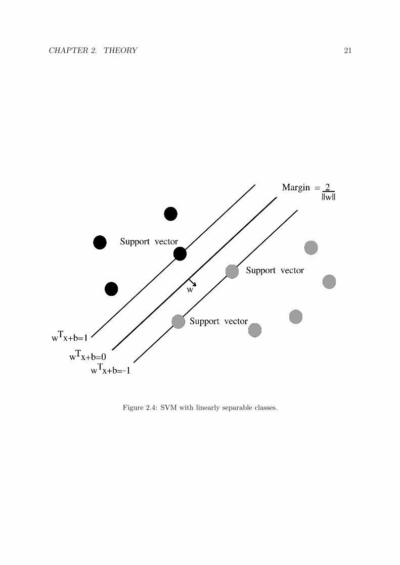
The basic SVM algorithm finds a predictor that belongs to the family of linear predictors[2, p.202]. SVM searches for a separating hyperplane that not only makes sure that datapoints from different classes fall on different sides of the plane but also maximizes themargin between the plane and the closest points of each class. Larger margins shouldlead to better generalization and prevent overfitting in high-dimensional attribute spaces[10].
There are different types of SVM; Hard-SVM and Soft-SVM [2, p.202]. Hard-SVM as-sumes that the different classes are linearly separable and returns a hyperplane withmaximum margin. However, in many scenarios the classes are not linearly separable. Inthis case Soft-SVM is a better choice. Soft-SVM is a generalization of the Hard-SVMand allows for some misclassified data points.
The procedure to find a separating hyperplane is similar in both the hard and the softcase. A training dataset, S, of the form established in 2.3 is needed. In this case xi ∈ Rn
and yi ∈ {1,−1}. Assume that S contains L data-label pairs. Figure 2.4 shows theHard-SVM where the classes are linearly separable. The data points in the figure arein R2 but the following reasoning also applies for points in Rn. As can be seen in thefigure, yi(w · xi + b) ≥ 1 holds for all data points in the set. A support vector fulfillsw · x + b = ±1. Let x+ and x− be support vectors on either side of the separating planei.e w ·x+ + b = 1 and w ·x−+ b = −1. Now, the margin M can be calculated using
M =w
||w||· (x+ − x−) =
w · x+ −w · x−||w||
=1− b− (−1− b)
||w||=
2
||w||(2.11)
So the margin is inversely proportional to ||w||. Hence, by minimizing ||w|| the marginis maximized. The Hard-SVM can thus be formulated as the optimization problem
minw‖w‖2 (2.12)
subject to yi(w · xi + b) ≥ 1 i = 1, ..., L
As mentioned, the Soft-SVM is a generalization of the Hard-SVM. This generalizationallows the SVM algorithm to be used even if the classes are not linearly separable. Theextension is done by introducting slack terms, ηi ∈ R+ for every point such that if the

CHAPTER 2. THEORY 20
point is misclassified then ηi ≥ 1. The Soft-SVM formulation is
minw,ηi
‖w‖2 + C
L∑i
ηi (2.13)
subject to yi(w · xi + b) ≥ 1− ηi i = 1, ..., L
The parameter C is a regularization parameter that indicates the relative cost betweenmisclassified points and the width of the margin. With a small C, misclassified points caneasily be ignored which allows for a larger margin. A large C implies that it is importantto avoid misclassification even if this means that the margin will be smaller. If C = ∞,the Hard-SVM is acquired since no misclassifications are allowed.
With the help of a suitable penalty function Φ(w; xi, yi) it is possible to formulate equa-tion 2.13 in another way,
minw
1
2||w||2 + C
L∑i
Φ(w; xi, yi) (2.14)
The penalty function could be either Φ1(w; xi, yi) = max(1−yiw ·xi, 0) or Φ2(w; xi, yi) =max(1− yiw · xi, 0)2 .
2.4.3 Semi-Supervised Support Vector Machine (S3VM)
While the Soft-SVM extended the Hard-SVM, an algorithm known as S3VM extendsthe Soft-SVM [10]. The ordinary SVM algorithms assume that each data point that isused for training is labeled. S3VM only needs some of the data points to be labeled.When working with S3VM the set of labeled data is known as the training set and theunlabeled data is the working set. If the working set is empty the method becomes thestandard SVM algorithm. If the training set is empty, the method becomes a form ofunsupervised learning. Semi-supervised learning occurs when both the working and thetest set is non-empty. In S3VM, two constraints are added for each unlabeled point in thetraining set. One constraint calculates the misclassification error as if the point belongsto class 1 and the other as if the point belongs to class -1. The objective function thencalculates the minimum of the two possible misclassification errors. The S3VM problemformulation is
minw,b,η,ξ,z
‖w‖+ C
[L∑i=1
ni +L+K∑j=L+1
min(ξj, zj)
](2.15)
subject to yi(w · xi + b) + ηi ≥ 1 η ≥ 0 i = 1, ..., Lw · xi − b+ ξj ≥ 1 ξj ≥ 0 j = L+ 1, ..., L+K
−(w · xi − b) + zj ≥ 1 zj ≥ 0
CHAPTER 2. THEORY 21
Figure 2.4: SVM with linearly separable classes.

CHAPTER 2. THEORY 22
Figure 2.5: Example of the difference in the solutions found by SVM and the S3VM algorithms.The black and the grey data points belong to a positive and a negative class respectively. Theordinary SVM algorithm finds a separating boundary that maximizes the margin to the twoclasses. However, by including unlabeled data (white points), the boundary is adjusted to alsomaximize the margin with the respect to the unlabeled data points.
2.4.4 Parameter selection
In addition to a training set and a label set, the previously introduced algorithms dependon the parameter C. It is common to let this parameter be C for one class and C · Cpfor the other class. These parameters affect the final weight vector and have to chosenbefore the training session. In case the training set is very imbalanced, a careful choice ofparameters can be the difference between finding a good or a bad predictor. A commonmethod of finding suitable parameters is to perform a grid search with crossvalidation[7]. A grid search is performed by systematically testing various pairs of C and Cp andthen simply choose the pair that yielded the best predictor. However, to avoid the risk offinding a predictor that performs well only on the available dataset but poorly on otherdatasets (i.e an overfitted predictor), crossvalidation is recommended [7]. Crossvalidationensures that the predictor is found using one dataset but tested on another. This shouldbe a better indicator of the expected performance of predictor than if the predictor wastrained and tested on the same dataset.
It is also recommended that the initial grid search is performed on a coarse grid [7]. Afiner grid search should then be performed around the point(s) of best performance in thecoarse grid. Finer and finer searches can then be added if it is deemed beneficial.
A practical method for finding good parameters is to start with a coarse grid with ex-ponentially growing sequences of C and Cp [7]. For example C = (2−5, 2−3, ..., 215) andCp = (2−15, 2−13, ..., 23).
CHAPTER 2. THEORY 23
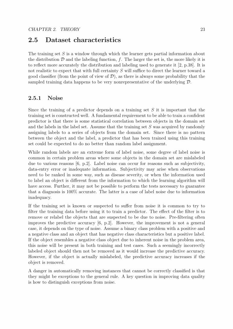
2.5 Dataset characteristics
The training set S is a window through which the learner gets partial information aboutthe distribution D and the labeling function, f . The larger the set is, the more likely it isto reflect more accurately the distribution and labeling used to generate it [2, p.38]. It isnot realistic to expect that with full certainty S will suffice to direct the learner toward agood classifier (from the point of view of D), as there is always some probability that thesampled training data happens to be very nonrepresentative of the underlying D.
2.5.1 Noise
Since the training of a predictor depends on a training set S it is important that thetraining set is constructed well. A fundamental requirement to be able to train a confidentpredictor is that there is some statistical correlation between objects in the domain setand the labels in the label set. Assume that the training set S was acquired by randomlyassigning labels to a series of objects from the domain set. Since there is no patternbetween the object and the label, a predictor that has been trained using this trainingset could be expected to do no better than random label assignment.
While random labels are an extreme form of label noise, some degree of label noise iscommon in certain problem areas where some objects in the domain set are mislabeleddue to various reasons [6, p.2]. Label noise can occur for reasons such as subjectivity,data-entry error or inadequate information. Subjectivity may arise when observationsneed to be ranked in some way, such as disease severity, or when the information usedto label an object is different from the information to which the learning algorithm willhave access. Further, it may not be possible to perform the tests necessary to guaranteethat a diagnosis is 100% accurate. The latter is a case of label noise due to informationinadequacy.
If the training set is known or suspected to suffer from noise it is common to try tofilter the training data before using it to train a predictor. The effect of the filter is toremove or relabel the objects that are suspected to be due to noise. Pre-filtering oftenimproves the predictive accuracy [6, p.2]. However, the improvement is not a generalcase, it depends on the type of noise. Assume a binary class problem with a positive anda negative class and an object that has negative class characteristics but a positive label.If the object resembles a negative class object due to inherent noise in the problem area,this noise will be present in both training and test cases. Such a seemingly incorrectlylabeled object should then not be removed as it would increase the predictive accuracy.However, if the object is actually mislabeled, the predictive accuracy increases if theobject is removed.
A danger in automatically removing instances that cannot be correctly classified is thatthey might be exceptions to the general rule. A key question in improving data qualityis how to distinguish exceptions from noise.

Chapter 3
Datasets and tools
The theoretical training dataset S that is needed to find a predictor was introduced insection 2.3. Section 3.1 describes the general structure of the realizations of S that areused in this project. Detailed information about the three datasets that are used as a basisfor the evaluations in chapter 6 is found in section 3.2. In section 3.3 some informationabout the development environment and external packages used in the implementationof the new training algorithm is presented.
3.1 The dataset structure
A typical fingerprint sample database at Precise Biometrics is constructed using a setof volunteers who provide multiple samples from multiple fingers. They provide bothenrollment and verification samples. In case a sensor is not large enough to cover thewhole fingerprint, the volunteers are instructed to move the finger between each samplecapture to make sure at least one sample from each part of the fingerprint has beencaptured at some point.
By creating a template from each of the enrollment samples collected from a single finger,a set of templates known as a multitemplate is formed, denoted T = {T1, ...,Tk}. A setof verification templates is denoted I = {I1, ..., Il}. A fingerprint template database thenconsists of a collection of pairs (T ,I), collected from each finger from each person. Afeature vector is acquired by using the α function introduced in section 2.1 on two tem-plates. The set of feature vectors acquired by matching a verification template with all thetemplates in a multitemplate is called a multifeature and is denoted F = α(T , I).
A training set S can now be created by repeatedly selecting a verification template anda multitemplate from two of the fingers in the database and creating a multifeature fromthese using the α function. If the verification template and the multitemplate comes fromthe same finger, the feature vectors in the resulting multifeature will all be consideredgenuines, otherwise they will be considered impostors. In this project, yi = 1 is the labelfor genuines and impostors are yi = −1. The dataset S is a set of labeled multifeaturesS = {(F1, y1), ..., (Fk, yk)}. Let F denote a single feature vector. Since a multifeature is
24

CHAPTER 3. DATASETS AND TOOLS 25
just a set of feature vectors where all feature vectors have the same label, it is also possibleto view S as a collection of labeled single feature vectors S = {(F1, y1), ..., (Fk, yk)}.
If one views S as a set of labeled feature vectors, S is in many cases going to contain ahigh degree of noise. This is because of the situation described in section 1.4; due to thesmall sensor size, each genuine multifeature is going to contain feature vectors that willresemble impostor feature vectors but they will nonetheless be labeled genuine (i.e yi = 1)in S. The level of feature noise in S depends on how evenly distributed the templates inthe multitemplates are over the fingers. Other factors that contribute are the size of thesensor as well as the number of templates in the multitemplates.
3.2 The datasets
The results of the changes made to the original training algorithm in this project areevaluated on three different datasets of different sizes. These datasets are referred to asSA, SB and SC . The following subsections present some specifics about the datasets.
3.2.1 Dataset SA
Dataset SA consists of feature vectors from Np = 50 people. Each person contributedwith samples from Nf = 6 fingers and Ne = 35 samples per finger during the enrollmentphase. They also provided Nv = 10 verification samples per finger. This gives a totalof NG = Np · Nf · Ne · Nv = 105000 genuines. When creating the impostors, no featurevectors from different fingers from the same person were included and only the firstverification template from each finger was used. Thus the number of impostors wereNI = Np · (Np − 1) · N2
f · Ne = 3087000. The number of multifeatures are 91200; 3000genuine and 88200 impostor multifeatures.
3.2.2 Dataset SB
The next dataset consists of feature vectors from 94 people and so called super impostors.These are impostors that have very similar features compared to genuines so they areeasily mistaken. However, the number of samples provided per finger is variable so aconcise expression for the number of genuines and impostors in this set is not as easilyprovided. The number of genuines are 223872 and impostors 11784960 spread out on6996 genuine and 368280 impostor multifeatures.
3.2.3 Dataset SC
Dataset SC contains feature vectors from 98 people. The number of genuines are 784000and impostors 4792200. These are spread out on 39200 genuine and 239610 impostormultifeatures.

CHAPTER 3. DATASETS AND TOOLS 26
3.2.4 Match information
Each feature vector in the datasets has a 7-dimensional numerical vector that containsinformation about the two templates that were used when creating the feature vector.Table 3.1 describes the information in the vector. The match information can be used topartition the dataset into training and test sets in such a way that no fingers from thesame person ends up in both the training and the test set. The match information is alsoused to construct the label set Y .
Column Description1 ID of the person who is the owner of the enrollment template.2 ID of the finger of the person who is the owner of the enrollment template.3 Index of the enrollment template.4 ID of the person who is the owner of the verification template.5 ID of the finger of the person who is the owner of the verification template.6 Index of the verification template.7 The match score given by a score function.
Table 3.1: Match information.
3.2.5 Memory limitations
When working on large datasets, it is necessary to consider the memory limitations ofthe computer architecture in use. In Matlab/Octave the datasets are represented usingdouble precision floating point format, i.e 8 bytes. With datasets containing severalmillions of elements, it can be impossible to load the whole dataset into memory. Table3.2 shows the sizes of the datasets. Both the original training algorithm in chapter 4 andthe new algorithm in chapter 5 work around this issue. The evaluations in chapter 6 areperformed on a computer with 12GB RAM.
Dataset Rows Columns Elements Approx size in RAM (GB)SA 3192000 114 363888000 3SB 12008832 128 1537130496 12SC 5576200 120 669144000 5
Table 3.2: Dataset sizes.

CHAPTER 3. DATASETS AND TOOLS 27
3.3 Tools
The following are the important tools used in this project.
3.3.1 Matlab/Octave
MATLAB (matrix laboratory) is a multi-paradigm numerical computing environmentand fourth-generation programming language. A proprietary programming language de-veloped by MathWorks, MATLAB allows matrix manipulations, plotting of functionsand data, implementation of algorithms, creation of user interfaces, and interfacingwith programs written in other languages, including C, C++, C#, Java, Fortran andPython.1
GNU Octave is software featuring a high-level programming language, primarily in-tended for numerical computations. Octave helps in solving linear and nonlinear prob-lems numerically, and for performing other numerical experiments using a language thatis mostly compatible with MATLAB. It may also be used as a batch-oriented language.Since it is part of the GNU Project, it is free software under the terms of the GNUGeneral Public License.2
3.3.2 LIBLINEAR
LIBLINEAR is a library for large linear classification developed by the machine learninggroup at National Taiwan University [3]. It is designed to efficiently handle data withmillions of instances and features and can be integrated into MATLAB/Octave.
LIBLINEAR supports two popular binary linear classifiers: logistic regression (LR) andlinear support vector machine (SVM). Given a set of instance-label pairs (xi, yi), i =1, ..., l, xi ∈ Rn, yi ∈ {−1, 1}, both methods solve the following unconstrained optimiza-tion problem with different penalty functions Φ(w;xi, yi),
minw∈Rn
1
2||w||p + C
∑k=1
Φ(w;xi, yi) (3.1)
where C > 0 is a penalty parameter. For SVM the two common penalty functions aremax(1− yiw ·xi, 0) and max(1− yiw ·xi, 0)2. These two types are known as L1-SVM andL2-SVM respectively. For LR the loss function is log (1 + e−yiw·xi).
1https://en.wikipedia.org/wiki/MATLAB2https://en.wikipedia.org/wiki/GNU Octave

CHAPTER 3. DATASETS AND TOOLS 28
3.3.3 SVMLIN
SVMLIN is a software package for linear SVMs created by Vikas Sindhwani at the Depart-ment of Computer Science at the University of Chicago [12]. SVMLIN can also utilizeunlabeled data and thus implements the S3VM algorithm introduced in section 2.4.3.The usage is very similar to LIBLINEAR as SVMLIN also has a MEX-wrapper whichmakes it available to MATLAB users.
3.3.4 FLANN
FLANN is a library developed by Marius Muja and David G. Lowe at the computerscience department at University of British Columbia [9]. The library performs fast ap-proximate nearest neighbor searches in high dimensional spaces. This library providesabout one order of magnitude improvement in query time over the best previously avail-able software.

Chapter 4
The original algorithm
This chapter introduces Precise Biometrics’ current training algorithm, AP (S), for thematching module. Section 4.1 expands on the theory established in chapter 2. Section4.2 looks at the specifics of the original training algorithm.
4.1 Introduction
The focus in this project lies on the matching module; more specifically, on the second andthird sub-modules as introduced in section 1.1. In section 2.1, these sub-modules wereformalized using the λ(F) function that makes a binary decision given a feature vectorF that contains the similarity information of two templates. The λ function should ofcourse be such that the correct decision is given with high probability.
Section 2.1 describes the λ function as a composite of the functions β and γ. The βfunction produces a similarity score given a feature vector, while the γ function makesa binary decision given a similarity score. These functions have previously only beenintroduced in terms of domains and co-domains but will now be explored further.
The β and γ functions used by Precise Biometrics are on the forms β(F; w) = F ·w andγ(s; t) = sgn(s−t). Thus, λ(F; w, t) = γ(β(F; w)−t) = sgn(F·w−t) which is recognizedas a linear predictor, due to section 2.4.1. Section 2.3 introduced the concept of trainingdata S and a training algorithm A(S) as objects needed to find a predictor. The detailsof the training data that is used by Precise Biometrics was specified in section 3.1. Thischapter explores Precise Biometrics’ training algorithm, denoted AP . The details of thefunctions that are used in the implementation of AP can be found in section 8.1. Thesedetails are best understood after reading this chapter.
29

CHAPTER 4. THE ORIGINAL ALGORITHM 30
4.2 The training algorithm AP
Since λ is a linear predictor it would be natural to use one of the linear training algorithms,AL, presented in section 2.4 on a dataset S to find a predictor. However, one immediatelyencounters a few issues when using this approach. First, the datasets used in this projectand by Precise Biometrics in general are, as seen in section 3.2.5, on the scale of millionsof feature vectors. The biggest dataset that is considered in this project takes up 12 GBwhen loaded into memory. With the computer setup used in this project it is unfeasibleto work directly on datasets of this magnitude.
Secondly, the predictor should generalize between fingers, meaning that it should notwork just on one specific kind of finger but on many. Therefore the performance of thepredictor on the individual feature vectors in S should not hold the same importance ashow well it does on the multifeatures. Also, as explained previously, the genuine featurevectors in S can be expected to contain a high degree of noise due to lack of overlapbetween verification templates and most templates in multitemplates.
Third, the AL algorithms both need two hyperparameters C and CP and there is nouniversal rule on how to choose these parameters.
To somewhat relieve the first two issues, the first step in AP is to extract a subset U ⊂ S.This is done by using the function
µP (F ; β) = argmaxF∈F
β(F) (4.1)
on every multifeature, Fk, in S. This function selects the highest scoring feature vectorin a multifeature where the score is calculated according to a score function β. Hence, Ucontains one vector from each multifeature. Depending on the number of multifeatures inS, the subset U can be considerably smaller. In section 3.2 the difference in size betweenS and U for the datasets used in this project can be seen. In addition to reducing thesize of the dataset, µP also acts as a filter for removing some noise depending on the βfunction used.
U is then used as input to an inner training algorithm, AP (U), the details of which
can be found in section 4.2.1. This algorithm returns the linear predictor λP and thecorresponding score function βP . It is thus possible to select a new subset from S usingβP .
The AP algorithm consists of a few iterations like this were a subset is used to traina predictor that is used to select a subset. An initial score function β0
P produces thesubset/predictor progression
Un = µP (S; βn−1P ) (4.2)
λnP = AP (Un). (4.3)
Let the sequence of score functions after K iterations be B = (β1P , ..., β
KP ). The best
performing score function is then chosen as the final score function using
βP (B) = argminβ∈B
FRRµP (S,β)(β, t) (4.4)

CHAPTER 4. THE ORIGINAL ALGORITHM 31
The predictor returned by AP (S) is thus the predictor λP that corresponds to βP . Figure4.1 illustrates the training process.
4.2.1 The inner training algorithm AP
As described in the previous section, the input to the inner training algorithm, AP isthe subset U ⊂ S where S is the full dataset. The core of AP are calls to the algorithmASVM(E) for E ⊂ U . Along with a dataset, ASVM expects two hyperparameters, C andCp. Suitable parameters are found using the parameter selection method described insection 2.4.4, i.e. a crossvalidated grid search. The crossvalidation is a version of 10-foldwhere the subset E that is used as input to ASVM is 1/10:th the size of U . However,instead of using U\E for performance evaluation of ASVM(E) as would be expected fork-fold crossvalidation, U is used.

CHAPTER 4. THE ORIGINAL ALGORITHM 32
Subset selection (μP)
Start
Dataset (S)
End
Partition
Train AL
Evaluate
Parameter selection
Dataset (E)
Predictor
Dataset (V)
Train AL
Best parameters
Evaluate
Predictor selection
Predictor (λP)
Predictor (λP)Performance (FRR@FAR)
Dataset (U*)
Predictor (λP)
Predictor (λP)
Training algorithm (AP)
Inner training algorithm (ÂP)
Parameter search
Performance (FRR@FAR)
Dataset (U)
Dataset (U)
^
^
^
Figure 4.1: The algorithm AP . A subset U is selected from a dataset S. Then, U is used inthe inner algorithm AP to train a predictor λP . The predictor λP is found by performing acrossvalidated parameter search and then training a predictor on U with the parameters thatwere found. A new subset can be selected using λP . The predictor λP is evaluated on the newsubset. The new subset can also be used in AP to perform additional training iterations.

Chapter 5
The new algorithm
This chapter introduces the new training algorithm AN(S). Section 5.1 describes theoverall strategy motivating the changes. Section 5.2 contains the details of the newtraining algorithm. In section 5.3 and 5.4, the new data selection functions are presented.Section 5.5 describes a feature manipulation method that is outside the scope of thisproject but could nevertheless be interesting to consider.
5.1 Introduction
The objective of this project is to investigate if and how the original training algorithmAP can be improved. The main strategy in the quest for improving AP is to generalize thedata selection function µP . Since µP selects only one feature vector per multifeature, thereis a possibility that valuable information is lost. The functions used in the implementationof the new training algorithm, AN , are listed in section 8.2 along with some designmotivations.
5.2 The training algorithm AN
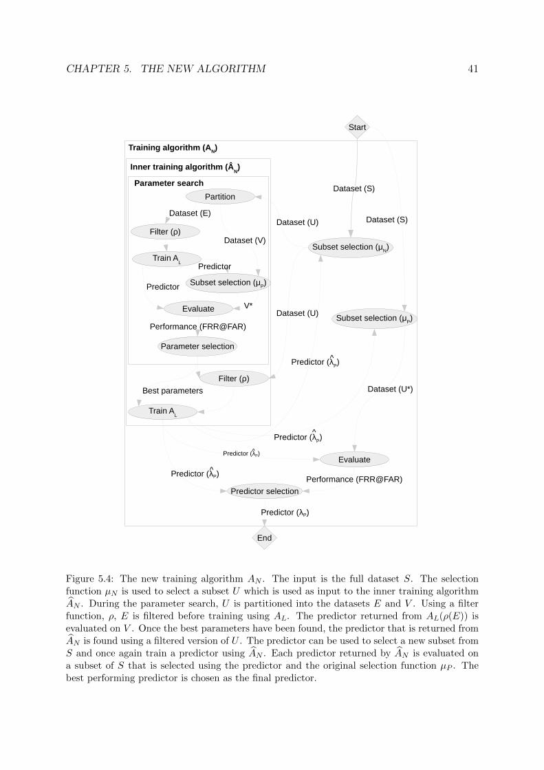
Similar to the original training algorithm AP , the input to the new training algorithmAN is a set S of of the form seen in section 3.1. The subset selection in the originaltraining algorithm was handled by the function µP which selects a subset U from the fulldataset S. In AN , this subset selection is handled using the new function µN(S) (detailsin section 5.3). Aside from µN and some changes in the implementation of AN in code,AN and AP is similar at this stage. The major changes are in the inner training algorithmAN . Figure 5.4 shows the structure of AN .
33

CHAPTER 5. THE NEW ALGORITHM 34
5.2.1 The inner training algorithm AN
As with the original inner training algorithm, AP , the input to the new training algo-rithm, AN , is a subset U of the full dataset S. In AN this subset is selected using µN .The algorithm returns the predictor λN = AN(U). Similar to AP , AN also employs acrossvalidated grid search method to find the hyperparameters C and Cp. However, the
subset E ⊂ U that was used as input to the AL algorithm in AP is first processed bya preprocessing function ρ(E) (section 5.4). Different ρ functions need a different set of
parameters. In the implementation of AN , the original grid search has been extended toalso include a parameter search for the selected ρ function.
A new AL algorithm is introduced in the new training structure, the S3VM algorithm(section 2.4.3). This method can handle a mixture of unlabeled and labeled data.
To achieve a good separation of training and test sets, the cross validation function hasbeen changed to employ a 50/50-split instead of the previous 90/100-split. This meansthat U is partitioned into two sets, E and V , of roughly equal size. Dataset E is used tofind the predictor AL(E) and V is used in the FRR calculation.
5.3 The selection function µN
The new training data selection method µN is an extension of the original µP function.While µP selects the highest scoring feature vector in a multifeature according to a scorefunction, µN allows selection of multiple of the highest scoring feature vectors from eachmultifeature. How many can also depend on whether the the multifeature is a genuineor an impostor. Three parameters are required for µN ; the number of genuines, NG, toinclude in E, the number of impostors, NI , to include in E and the number of genuinesand impostors, N , to include in V .
5.4 The filter functions ρ
This section introduces the new inner training data filter methods ρ(E) for the datasetE. These methods are classified as either additive or subtractive depending on whetherthey add or or remove data points from E.
The genuines are the minority class and should therefore be upsampled in some way. It ispossible to use both the additive and the subtractive methods to upsample the genuines,if the ρ methods are combined with a suitable µN method. By choosing a µN method thatselects many feature vectors from each genuine multifeature, for example the five highestscoring feature vectors instead of only the single highest, a subtractive ρ method couldthen be used to remove some elements from E. When using the additive ρ functions,E should however probably contain the best genuine candidates. By using the µN thatchooses only the highest scoring feature vector in each multifeature, one acquires a small

CHAPTER 5. THE NEW ALGORITHM 35
but confident dataset. By allowing more feature vectors per multifeature, a bigger butless confident dataset is acquired.
In the implementation of ρ (section 8.2), the subtractive methods do not actually removeelements from E. They merely relabel feature vectors from ±1 to 0 or 2 depending on themethod of choice. The implementation of the SVM algorithm ignores feature vectors thatare labeled 0 or 2. However, S3VM uses the 0-labeled vectors as unlabeled but ignoresthe 2-labeled vectors. The following subsections provide a description of the differentρ methods investigated during this project. Table 5.1 contains a brief summary of themethods.
Preprocessing method ρ TypeADASYN AdditiveSMOTE AdditiveGrey data SubtractiveMark below SubtractiveRandom downsampling SubtractiveRecursive SubtractiveVote Subtractive
Table 5.1: Data preprocessing methods used in this project.
5.4.1 ADASYN
Adaptive Synthetic Sampling Approach for Imbalanced Learning (ADASYN) generatesmore data for the minority class examples that are difficult to classify using a weighteddistribution. In [5] the ADASYN algorithm is described as follows:
ADASYN
InputTraining dataset Dtr with m samples {xi, yi}, i = 1, ...,m, where xi is an instance inthe n dimensional feature space X and yi ∈ Y = {−1, 1} is the class identity labelassociated with xi. Define ms and ml as the number of minority class examplesrespectively. Therefore, ms ≤ ml and ms +ml = m.
Procedure(1) Calculate the degree of class imbalance
d = ms/ml (5.1)
where d ∈ (0, 1].(2) If d < dth then (dth is a preset threshold for the maximum tolerated degree ofclass imbalance ratio):
(a) Calculate the number of synthetic data examples that need to be generated forthe minority class:
G = (ml −ms)× θ (5.2)

CHAPTER 5. THE NEW ALGORITHM 36
Where θ ∈ [0, 1] is a parameter used to specify the desired balance level aftergeneration of the synthetic data. θ = 1 means a fully balanced dataset is createdafter the generalization process.
(b) For each example xi ∈ minorityclass, find K nearest neighbors based on theEuclidean distance in n dimensional space, and calculate the ratio ri defined as
ri = ∆i/K, i = 1, ...,ms (5.3)
where ∆i is the number of examples in the K nearest neighbors of xi that belongto the majority class, therefore ri ∈ [0, 1];
(c) Normalize ri according to ri = ri/∑ms
i=1 so that ri is a density distribution(∑
i ri = 1).
(d) Calculate the number of synthetic data examples that need to be generated foreach minority example xi,
gi = r ×G (5.4)
where G is the total number of synthetic data examples that need to be generatedfor the minority class as defined in equation 5.2. (e) For each minority class dataexample xi, generate gi synthetic data examples according to the following steps:
– Do the Loop from 1 to gi
(i) Randomly choose one minority data example, xzi from the K nearest neigh-bors for data xi.
(ii) Generate the synthetic data example
si = xi + (xzi − xi)× λ (5.5)
where (xzi − xi) is the difference vector in n dimensional space, and λ is arandom number: λ ∈ [0, 1].
– End Loop
The key idea of the ADASYN algorithm is to use a density distribution ri as a criterionto automatically decide the number of synthetic samples that need to be generated foreach minority data example. ri is a measurement of the distribution of weights fordifferent minority class examples according to their level of difficulty in learning. Theresulting dataset post ADASYN will not only provide a balanced representation of thedata distribution (according to the desired balance level defined by the θ coefficient), butit will also force the learning algorithm to focus on those difficult to learn examples. Twoparameters are needed as input, θ and K.

CHAPTER 5. THE NEW ALGORITHM 37
5.4.2 SMOTE
Synthetic Minority Oversampling Technique (SMOTE) is a technique in which the minor-ity class (in this project, the genuines) is oversampled [4]. Instead of creating exact copiesof existing minority class samples like in a simple upsampling approach, SMOTE inter-polates between samples to create synthetic samples. The synthetic samples are createdby introducing a new sample along each of the lines connecting to the k nearest neighborsof each minority class sample. One parameter, a ∈ N is needed for this algorithm. Letthe number of genuines in the training set be NG. After applying this method, the newnumber of genuines will be NG = a ·NG.
Figure 5.1: The SMOTE algorithm. The black class is being upsampled. The five nearestneighbors to the point X are X1 through X5. A new data point is being introduced along thelines connecting to the neighbors.
5.4.3 Grey data
This function assigns the label 0 to all but the highest scoring vector in each multifeature.If E contains only the highest scoring features from all multifeatures, the functions doesnothing. Since the original SVM algorithm ignores vectors labeled 0, this function shouldbe used together with S3VM .
5.4.4 Mark below
Mark below calculates the average score, savg of the highest scoring 10% of genuines inE. Given a variable a ∈ R, the method then relabels data points whose score s is lessthan s < a · savg. The new label is 0.

CHAPTER 5. THE NEW ALGORITHM 38
5.4.5 Random downsampling
The random down-sampling approach is among the simpler approaches to class balanc-ing. This method randomly chooses data points to remove or reclassify. Unlike theup-sampling methods which are applied to the minority class, this method is applied tothe majority class. There are pros and cons with this method. A predictor’s confidenceand training time is generally positively correlated with the size of the dataset; a biggerdataset produces a more confident predictor but it takes longer to find it. The randomdown-sampling method removes data points randomly from the training set. Two pa-rameters are required as it is possible to remove points both from the genuines and theimpostors. Assume that the number of genuines and impostors in the training set isNG and NI respectively. Given parameters a, b ∈ (0, 1] the new number of genuines andimpostors are NG = a ·NG and NI = b ·NI .
5.4.6 Recursive
In [6] it is suggested that the same algorithm can be used to train both the predictor anda filter. This method thus finds a predictor λL using AL(E). Then, λL (or rather its scorefunction βL) is applied to the same set E to remove the genuines with the worst score.The name of this method is due to it being implemented recursively, meaning that themethod allows for a filter to be found using AL(ρ(E)) when ρ is the recursive method.The parameter needed for this function is the number of recursive calls that should bemade. This method is illustrated in figure 5.2.
5.4.7 Voting filter
The K-nearest neighbors algorithm has, since 1972, been used extensively as a filtermethod [6]. The voting filter relabels a data point according to a majority vote amongits nearest nearest neighbors. If a majority of the neighbors surrounding a genuine areimpostors, the genuine is relabeled to 0. Two parameters are needed for this method; thenumber of neighbors to use and how many of those neighbors that need to be impostorsin order for the data point to be relabeled.

CHAPTER 5. THE NEW ALGORITHM 39
Filter (ρ)
E
Remove
Train AL
Predictor
E
E*
Filter (p)
E**
Figure 5.2: The recursive filter. Dataset E is used to train a predictor. The predictor is thenused to relabel or remove the points from E that were not classified correctly, thus creatingdataset E∗. Depending on recursive depth, E∗ can be used as input to the same filter.

CHAPTER 5. THE NEW ALGORITHM 40
5.5 Feature transformation
Note: the theory suggested in this section can not currently be easily implemented dueto Precise Biometrics’ system architecture. These changes are nevertheless interesting toconsider.
None of the algorithmic changes so far have made any transformations to the featurevectors in S. Selecting the feature vector with the highest score from each multifeatureis done under the assumption that the most characteristic information contained in themultifeature can be fairly well represented by this single vector. This is often true ifthe enrollment and the verification templates are from roughly the same parts of thesame finger so that there is a good amount of overlap. However, there is a risk that theverification template does not overlap one single enrollment template well. In this case theverification template may instead overlap several enrollment templates, but only partially.Selecting only the highest scoring feature vector to represent the whole multifeature couldthen be a bad representation of the multifeature characteristics.
A simple method of capturing some extra information about the multifeature that was im-plemented during this project is to concatenate each feature vector with its correspondingmultifeature centroid.
Figure 5.3: The centroid method. The stars are centroids of two multifeatures. In this figure,the features are in R2. Concatenating each feature with the centroid extends the features toR4.
CHAPTER 5. THE NEW ALGORITHM 41
Subset selection (μP)
Start
Dataset (S)
End
Partition
Train AL
Evaluate
Parameter selection
Dataset (E)
Predictor
Dataset (V)
Train AL
Best parameters
Evaluate
Predictor selection
Predictor (λP)
Predictor (λP)Performance (FRR@FAR)
Dataset (U*)
Predictor (λP)
Training algorithm (AN)
Inner training algorithm (ÂN)
Parameter search
Performance (FRR@FAR)
Dataset (U)
Dataset (U)Filter (ρ)
Subset selection (μN)
Dataset (S)
Filter (ρ)
Subset selection (μP)
Predictor
V*
Predictor (λP)
Predictor (λP)
^
^
^
^
Figure 5.4: The new training algorithm AN . The input is the full dataset S. The selectionfunction µN is used to select a subset U which is used as input to the inner training algorithmAN . During the parameter search, U is partitioned into the datasets E and V . Using a filterfunction, ρ, E is filtered before training using AL. The predictor returned from AL(ρ(E)) isevaluated on V . Once the best parameters have been found, the predictor that is returned fromAN is found using a filtered version of U . The predictor can be used to select a new subset fromS and once again train a predictor using AN . Each predictor returned by AN is evaluated ona subset of S that is selected using the predictor and the original selection function µP . Thebest performing predictor is chosen as the final predictor.

Chapter 6
Results
This chapter presents the effects of the changes made to the algorithm AP during thisproject. Section 6.1 describes how these effects are measured. Section 6.2 - 6.5 presentsthe results.
6.1 Evaluation procedure
When creating the algorithm AN , the old algorithm AP was used as a base. The changesmainly consist of the new selection function µN (section 5.3), the preprocessing functionsρ (section 5.4) and the additional AL algorithm S3VM . By varying the parameters of theµN function along with different combinations of ρ functions and AL algorithms, differentversions of the AN algorithm are acquired. This chapter is dedicated to investigating theperformance of some versions of AN .
The predictors (or rather the associated score functions) returned by the different versionsare evaluated with the FRR@FAR measure (section 2.3.1). To calculate the FRR@FARfor a predictor, a few things are required. Beyond the predictor itself one also needs tospecify the desired FAR level and provide a dataset to test the predictor on. A goodpredictor should give low FRR on a low FAR level but due to the size of the datasetsin this project it is not possible to calculate a confident FRR on very low FAR levels.The predictors in this project are thus evaluated using FRR@1/10000. Table 6.1 showshow many falsely accepted impostors this actually implies for the different datasets SA,SB and SC used in this project. The most confident results are therefore going to be theones acquired from dataset SB and the least from SA.
Dataset Impostor multifeatures False accepts at FAR=1/10000SA 88200 8SB 368280 36SC 239610 23
Table 6.1: False accepts for the different datasets.
42

CHAPTER 6. RESULTS 43
The dataset that is used when calculating FRR@FAR for a predictor should be selectedwith care. It is important that a predictor performs well on data points it has neverencountered before since this is the situation that the predictor will experience in thereal world. Crossvalidation is often used in order to simulate new data. However, thistechnique requires multiple training sessions. Depending on the dataset S and the settingsused for AN , the search for a predictor AN(S) can take a long time, sometimes days.The FRR@FAR values in section 6.2 are therefore calculated using the same datasetas used for training. This method is also the preferred method by Precise Biometricswhen measuring the performance of a predictor and should be at least indicative ofthe performance that would be acquired by crossvalidation. An estimate of the differencebetween the performance reported by a non-crossvalidated versus a crossvalidated methodis provided in section 6.4.
6.1.1 The baseline
To investigate whether or not the changes made to AP during this project have any kindof effect it is important to have a baseline to compare against. The goal of this projectis to examine if some dataset processing could be included in the training algorithm soas to reliably achieve a better performing predictor. In AP , some dataset processing isalready done through µP . The ρ functions and the S3VM algorithm are however newto this project. The baseline algorithm hence utilizes the µP function but no ρ function.Furthermore, the AL algorithm used in the original training algorithm is SVM. Thesesettings are considered the baseline.
6.1.2 Parameters for the ρ and µN functions
Some of the ρ functions require one or a set of parameters to specify how to processa dataset. Through the new parameter search method (section 5.2.1) these parameters
can be included in the crossvalidated grid search in AN , along with the hyperparametersrequired for the AL algorithms.
While the µN parameters also can be included in the new parameter search method, therange of suitable parameters is small; since the subset U ⊂ S that is selected from S isloaded into RAM, U should not be too big. The inner training algorithm AN includes acrossvalidation step when searching for hyperparameters. However, this ensures that thepredictor returned by the inner training algorithm AN(U) does not overfit on dataset U .Depending on how well U represents the characteristics of S this could also imply thatthe predictor does not overfit on S. To hopefully increase the chance that the importantcharacteristics in S are also in U one can include more feature vectors per multifeaturein U using the µN function.
The three parameters needed for the µN function are in this chapter denoted NG, NI andN as introduced in section 5.3.

CHAPTER 6. RESULTS 44
6.1.3 Initial subset
The initial subset U1 ⊂ S in AN depends on an initial score function β0N . Each feature
vector in the datasets used in this project is connected to a score that has been assignedby a previous score function, βP . This is the score function given by a few iterations in theoriginal AP algorithm. A possible initial subset could then be selected using the scores inthe datasets. In this case, AN could be considered as a continuation of AP . However, ifAN is to be considered as a replacement for AP it is informative to also examine to whatextent AN :s performance depends on the initial score function. This is evaluated by alsoperforming tests using a random initial score function βR.
6.2 Algorithmic performance using β0N = βP
By using β0N = βP to select U1 using the µN function it can be expected that the initial
selection is already relatively good so only a few iterations in AN should be needed. Thenumber of iterations are set to 10. The tests are also performed using a parameter searchfor the ρ functions that need it. This parameter search is, however, not extensive inorder to keep the training time down. Instead, each ρ function is supplied with a smallset of parameter candidates among which the parameter search method selects the bestsuited. The results of this case are presented in table 6.2. The baseline algorithm ishighlighted with blue. The best settings found on each dataset is highlighted with green.Since tests using dataset SC can take days to complete for some settings, some tests arenot performed on this dataset. The tests on SC were mostly performed after observing agood result for some settings on SA or SB.
As seen in table 6.2, there are settings that perform better than the baseline settings.There is however no setting that manages to considerably outperform the baseline for allthree datasets. The setting that seems to have the highest chance of providing a universalimprovement is to switch from ASVM to AS3VM , use a recursive filter and performing theparameter search on the five highest scoring feature vectors in each multifeature. Thissetting manages to outperform the baseline on both SA and SC while the result on SB issomewhat improved.
Increasing N (and thereby increasing the resemblance between subset U and dataset S
when performing evaluations in AN) seems to provide a slight increase in performance,at least when using ASVM . As could be expected, increasing NG from 1 to 2 or 5 withoutalso including some ρ function decreases the performance since this introduces noise thatis not filtered out.
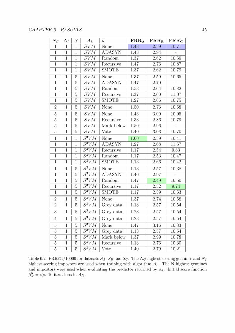
CHAPTER 6. RESULTS 45
NG NI N AL ρ FRRA FRRB FRRC
1 1 1 SVM None 1.43 2.59 10.711 1 1 SVM ADASYN 1.43 2.94 -1 1 1 SVM Random 1.37 2.62 10.591 1 1 SVM Recursive 1.47 2.76 10.871 1 1 SVM SMOTE 1.37 2.62 10.79
1 1 5 SVM None 1.37 2.59 10.651 1 5 SVM ADASYN 1.47 2.70 -1 1 5 SVM Random 1.53 2.64 10.821 1 5 SVM Recursive 1.37 2.60 11.071 1 5 SVM SMOTE 1.27 2.66 10.75
2 1 5 SVM None 1.50 2.76 10.58
5 1 5 SVM None 1.43 3.00 10.955 1 5 SVM Recursive 1.33 2.86 10.795 1 5 SVM Mark below 1.50 2.96 -5 1 5 SVM Vote 1.40 3.03 10.70
1 1 1 S3VM None 1.00 2.59 10.411 1 1 S3VM ADASYN 1.27 2.68 11.571 1 1 S3VM Recursive 1.17 2.54 9.831 1 1 S3VM Random 1.17 2.53 10.471 1 1 S3VM SMOTE 1.13 2.66 10.42
1 1 5 S3VM None 1.13 2.57 10.381 1 5 S3VM ADASYN 1.40 2.97 -1 1 5 S3VM Random 1.47 2.49 10.501 1 5 S3VM Recursive 1.17 2.52 9.741 1 5 S3VM SMOTE 1.17 2.59 10.53
2 1 5 S3VM None 1.37 2.74 10.582 1 5 S3VM Grey data 1.13 2.57 10.54
3 1 5 S3VM Grey data 1.23 2.57 10.54
4 1 5 S3VM Grey data 1.23 2.57 10.54
5 1 5 S3VM None 1.47 3.16 10.835 1 5 S3VM Grey data 1.13 2.57 10.545 1 5 S3VM Mark below 1.37 2.99 10.785 1 5 S3VM Recursive 1.13 2.76 10.305 1 5 S3VM Vote 1.40 2.79 10.21
Table 6.2: FRR@1/10000 for datasets SA, SB and SC . The NG highest scoring genuines and NI
highest scoring impostors are used when training with algorithm AL. The N highest genuinesand impostors were used when evaluating the predictor returned by AL. Initial score functionβ0N = βP . 10 iterations in AN .

CHAPTER 6. RESULTS 46
6.3 Algorithmic performance using β0N = βR
If one instead selects U1 using a random initial score function, i.e β0N = βR, the results
in table 6.3 are acquired. Comparing the FRR of each setting in table 6.3 with thecorresponding FRR in table 6.2 suggest that AN might be able to manage without aninitial score provided by AP since the acquired FRR values are similar to those acquiredwhen using β0
N = βP . The new training algorithm AN should therefore be able to functionas replacement for AP and not just a continuation.
Table 6.3 also reports the training times when using AN on the different datasets. Forthe big and complex dataset SC , this time is several hours. During some test runs itwas observed that for SC most of this time was spent in AL. Another test using therandom downsampling ρ function was therefore performed in an effort to bring down thetraining time. As table 6.3 shows, the training time is indeed reduced when using randomdownsampling for all datasets while still maintaining similar FRR values compared to theno ρ function case. If one accepts a slight FRR difference, the training time should thusbe able to be reduced.
NG NI N AL ρ FRRA FRRB FRRC TA TB TC
1 1 1 SVM None 1.53 2.64 10.70 17 133 7351 1 1 SVM Random 1.40 2.70 10.69 11 90 921 1 1 S3VM None 1.07 2.62 10.46 43 237 10451 1 1 S3VM Random 1.23 2.53 10.49 17 73 118
Table 6.3: FRR@1/10000 for datasets SA, SB and SC . The training times TA, TB and TC arein minutes. The NG highest scoring genuines and NI highest scoring impostors are used whentraining with algorithm AL. The N highest genuines and impostors were used when evaluatingthe predictor returned by AL. Initial score function β0N = βR. 10 iterations in AN .
6.3.1 Convergence
The interior of algorithms AP and AN both produce a sequence of score functions B =(β1, ..., βn) as seen in section 4.2. By measuring the performance of these score functionson the full dataset S, a sequence of FRR@FAR values is acquired. This sequence can beused to evaluate the convergence of AN for specific settings. The sequence for datasetSB is shown in figure 6.1. The solid line represents the FRR evolution given the initialscore function β0
N = βP . The dashed line instead uses β0N = βR. After four iterations
the FRR values are roughly the same regardless of the initial score function used. Thesettings that are used are NG = NI = N = 1 and ASVM and no ρ function.

CHAPTER 6. RESULTS 47
Figure 6.1: Convergence for dataset SB with NG = NI = N = 1, ASVM and no ρ function.Solid line is training using the initial score function β0N = βP while dashed uses β0N = βR. 10training iterations in AN .
6.4 Overfitting
The implementation of the new training algorithm includes an evaluation method thatmeasures the degree of overfitting experienced in AN(S). This method uses a 5 × 2-crossvalidation as seen in section 2.3.3. Algorithm AN is thus evaluated ten times ondifferent datasets. The subset S1 ⊂ S is used to find the predictor λN returned byAN(S1). Another subset S2 ⊂ S is then used to evaulate the performance of λN . Sincethe crossvalidation method is 5× 2 the subsets S1 and S2 are (roughly) equal in size anddisjoint. The settings used for AN are the same as in section 6.3.1. Datasets SB and SCwere used for this evaluation.
For SB, the mean difference of the performance measured on S2 compared to S1 is 1.60%using β0
N = βP and 1.07% using β0N = βR. For SB, these numbers are 0.54% and 0.61%
respectively. Thus, AN does seem to experience some overfitting using these settings,more so on dataset SB compared to SC .

CHAPTER 6. RESULTS 48
6.5 Feature transform - Centroid method
Section 5.5 introduced a feature transformation method which consisted of appending themultifeature centroid to the feature vectors in the dataset. As noted, this theory can notbe easily implemented due to the surrounding architecture of Precise Biometrics’ system.Hence, no extensive testing has been done with this method. However, the method wastested on dataset SA with ASVM , the original selection function µP and no ρ and 10training iterations. The centroid method achieved a FRR@1/10000 of 0.33%. This isconsiderably better than the results presented for SA in section 6.2. The centroid datasetwas generated from SA through a function that could easily handle a set of SA:s size. Togenerate similar datasets from SB and SC would require a modification of this functionbut since the centroid method was deemed unimplementable due to the surroundingsystem architecture, similar tests for SB and SC were not performed.

Chapter 7
Conclusions
None of the dataset processing techniques explored in this project is able to considerablyimprove on the originally used technique on all three datasets. The ρrecursive function forexample, produces the best results among the tested ρ functions on dataset SC . The samegood performance can, however, not be seen on the other datasets using this function. Itmight be the case that a more careful parameter search could make a technique performwell on a general dataset. However, the reason for not doing an extensive ρ functionparameter search in this project was simply due to the considerable time it would take. Itcould therefore be beneficial to explore methods of reducing the training times. One suchmethod that was explored in this project was to downsample the impostors randomly.This reduced the training time while still maintaining a similar performance comparedto the baseline.
The downsampling method reduces the time spent in the AL algorithms. Another majortime sink observed when implementing AN was the loading of large amounts of data fromdisk to memory. A time efficient algorithm implementation should thus avoid unnecessaryloadings. For precise memory control, Matlab/Octave might not be the best choice oflanguage.
The performance of AN does not seem to be heavily influenced by the initial subsetselection when using the baseline settings so it should be able to function as a replacementfor AP .
7.1 Future work
7.1.1 Feature transformation
The centroid method presented in section 5.5 showed promising results on dataset A.Even though it is not possible at the moment to implement this technique due to PreciseBiometrics’ surrounding system architecture it could be interesting to investigate thistechnique on bigger datasets in case it proves to be a successful technique. The centroidtechnique suggest that there might be other, better ways of capturing the characteristics of
49

CHAPTER 7. CONCLUSIONS 50
a multifeature compared to simply choosing one of the feature vectors in the multifeatureaccording to some criteria as is done today.
7.1.2 Robust SVM
During the final stages of this project an interesting paper named Support Vector Ma-chines Under Adversarial Label Noise was found [8]. This paper presented a robust SVM,meaning an SVM that was built under the assumption that the labels contain noise. Therobust SVM is formulated using a modification of the ordinary SVM dual problem withonly a relatively simple modification of the kernel. It is reported to not add much com-plexity beyond the original SVM.
Chapter 8
Appendix
The appendix contains descriptions of functions and function dependencies from theoriginal and the new training structure. Provided is also a usage example for the newtraining structure.
8.1 The original training structure
This section contains the implementation details of the original training algorithm AP .This algorithm is implemented using a mixture of Matlab/Octave and C functions. The
subset selection µP is implemented in C while the inner training algorithm AP usesMatlab/Octave functions with the exception of AL which uses the LIBLINEAR package
(i.e C/C++). Algorithm AP corresponds to the function pb ml train in the list offunctions in section 8.1.1.
8.1.1 Functions
The following are short descriptions of the Matlab/Octave functions in the implemen-
tation of AP . These can also be found in figure 8.1 where arrows indicate functiondependencies.
pb ml trainThe main function for the inner algorithm A. Trains a predictor given a dataset.
pb ml filter featuresRemoves feature dimensions that have the same value for all instances in the trainingset.
pb ml load featuresLoads the training set from .txt files.
pb ml normalize featuresNormalizes the features using the method of choice.
51

CHAPTER 8. APPENDIX 52
pb ml print modelPrints weight vector and the scale parameters of the trained predictor to a C-file for usein the next step in the training loop.
pb ml train modelControl function for the hyper-parameter search and crossvalidation.
pb ml crossvalidatePerforms a crossvalidation over a grid of hyper-parameters given a set of hyper-parameters.
pef plot roc simplePlots a ROC curve for a predictor.
pb ml liblinear predict Predicts labels for a dataset given a linear predictor.
pef compute frr at farComputes FRR given a predictor, dataset and a FAR value.
pb ml liblinear train Wrapper function for the LIBLINEAR package. Trains a predic-tor given a training set.

CHAPTER 8. APPENDIX 53
8.2 The new training structure
Nearly every function that forms the implementation of the original training algorithmAP has been changed when designing and implementing the new training algorithm, ANalthough the general structure is the same. The modifications and additions to AP weremade with two criteria in mind; speed and versatility. When working with datasets of themagnitude seen in this project, poorly designed functions could slow down the trainingtime considerably. Hence, whenever possible, functions were constructed using a timesaving design. To achieve a better versatility, AP , was modified according to a plug andplay philosophy so that ρ and AL functions could easily be switched. This would alsomake it easy to investigate new such functions after this project has ended.
A major new feature in the implementation ofAN is that all the code is gathered under onemain function. In the original training structure, the function pb ml train implementsAP . In the new training structure pb ml train corresponds to AN while the innertraining algorithm, AN is implemented using pb ml train model.
Collecting the entire training process under one main function makes it easier for usersto handle to training process.
8.2.1 Functions
The following are short descriptions of the important functions in the new training struc-ture. These can also be found in figure 8.2 where arrows indicate function dependen-cies.
pb ml trainThe main function for the training algorithm AN . Trains a predictor given a dataset.
calculate scoresAssigns a score to each point in a dataset.
pb ml predictCalculates a score for each point in a dataset.
pb ml predict linear scoreMEX-wrapper for the C function pb ml predict linear score
add dataset infoExtracts information such as the number of people, fingers, enrollment templates andverification templates.
pb ml train modelThe main function for the inner training algorithm AN .
new original searchInitialization method for the grid search for the parameters required in the AL algo-rithms.

CHAPTER 8. APPENDIX 54
grid searchSearches for best parameters among a given set.
pb ml crossvalidateCrossvalidation function.
cont evalCalculates FRR from a set of scores.
partition 50 50Partitions a dataset into two (roughly) equally sized parts.
select subsetSelects a training and test set according to the given NG, NI and N parameters (section5.3).
select training dataFilters the training data according to the chosen ρ function.
recursiveThe recursive ρ function.
flann selectThe majority vote ρ function.
SMOTEThe SMOTE ρ function.
ADASYNThe ADASYN ρ function.
random samplingThe random downsampling ρ function.
mark belowThe mark below ρ function.
get modelTrains using the selected linear training algorithm AL.
compute rankRanks the features in each multifeature with respect to a score function.

CHAPTER 8. APPENDIX 55
8.2.2 An example
Algorithm AliasSupport Vector Machine linear svmSemi-Supervised Support Vector Machine linear svm semi supervisedLogistic Regression linear lr
Table 8.1: Available algorithms and corresponding code alias.
The following table contains the pre-processing methods that have been implementedduring this project. Vectors in this table are row vectors. Further explanations of thesemethods are referred to section 5.4.
Method Alias Parameter format Parameter rangeSMOTE smote a a ∈ N+
ADASYN adasyn [a b] a ∈ N+, b ∈Grey data delabel - -Random downsampling random [a b] a, b ∈ (0, 1]Recursive recursive a a ∈ N+
Mark below mark below a a ∈ RVote flann [a b] a, b ∈ N+, a ≥ b ∈ (0, 1]
Table 8.2: Pre-processing methods.

CHAPTER 8. APPENDIX 56
The following is a MATLAB script showing an example of how to specify options andwhat type of options that can be specified in the new training environment.
1 % Folder with genuines and impostors files.
2 options.folder=’./Features/dataset_a’;
3 % Number of highest genuines and impostors to test
4 % on in each crossvalidation iteration.
5 options.test_on_max=1;
6 % Number of highest genuines to train
7 % on in each crossvalidation iteration.
8 options.training_set_genuines=1;
9 % Number of highest impostors to train
10 % on in each crossvalidation iteration.
11 options.training_set_impostors=1;
12 % Model to use during training.
13 options.modeltypes=’linear svm’;
14 % Training data selection method.
15 options.data_selectors=’flann’;
16 % Parameters to use for training data selection.
17 options.training_ops=[5 2];
18 % Number of crossvalidation iterations to use.
19 options.crossval_folds=10;
20 % Number of training iterations to run.
21 options.training_iterations=10;
22 % Number of evaluation iterations to run.
23 options.evaluation_iterations=0;
24 % FAR level to evaluate the results on.
25 options.fars=[1/10000];
26 % Level of console outputs during training.
27 options.verbosity=2;
28 % Train using the square of each feature.
29 options.use_square=1;
30 % Use the standard deviation method to find
31 % scaling parameters.
32 options.use_std=1;
33 % Block size to read into memory (approximate).
34 options.block_size_bytes=1e9;
35 % Use random initial subset selection.
36 options.initial_zero_score=0;
37 % Run test
38 [frrs,ref_frr,eval_frr,time,w,scale,discarded_cols]=pb_ml_train(options);

CHAPTER 8. APPENDIX 57
Fig
ure
8.1
:S
tru
ctu
reof
the
imple
men
tati
onofAP
.T
he
arro
ws
show
fun
ctio
nd
epen
den
cies
.

CHAPTER 8. APPENDIX 58
Fig
ure
8.2:
Str
uct
ure
ofth
eim
ple
men
tati
onofAN
.T
he
arro
ws
show
fun
ctio
nd
epen
den
cies
.

Bibliography
[1] Maltoni, Davide, et al. Handbook of fingerprint recognition. Springer Science & Busi-ness Media, 2009.
[2] Shalev-Shwartz, Shai, and Shai Ben-David. Understanding machine learning: Fromtheory to algorithms. Cambridge university press, 2014.
[3] Fan, Rong-En, et al. ”LIBLINEAR: A library for large linear classification.” Journalof machine learning research 9.Aug (2008): 1871-1874.
[4] Chawla, Nitesh V., et al. ”SMOTE: synthetic minority over-sampling technique.”Journal of artificial intelligence research 16 (2002): 321-357.
[5] He, Haibo, et al. ”ADASYN: Adaptive synthetic sampling approach for imbalancedlearning.” Neural Networks, 2008. IJCNN 2008.(IEEE World Congress on Computa-tional Intelligence). IEEE International Joint Conference on. IEEE, 2008.
[6] Brodley, Carla E., and Mark A. Friedl. ”Identifying mislabeled training data.” Journalof artificial intelligence research 11 (1999): 131-167.
[7] Hsu, Chih-Wei, Chih-Chung Chang, and Chih-Jen Lin. ”A practical guide to supportvector classification.” (2003): 1-16.
[8] Biggio, Battista, Blaine Nelson, and Pavel Laskov. ”Support Vector Machines UnderAdversarial Label Noise.” ACML 20 (2011): 97-112.
[9] Muja, Marius, and David G. Lowe. ”Fast approximate nearest neighbors with auto-matic algorithm configuration.” VISAPP (1) 2.331-340 (2009): 2.
[10] Bennett, Kristin, and Ayhan Demiriz. ”Semi-supervised support vector machines.”NIPS. Vol. 11. 1998.
[11] Refaeilzadeh, Payam, Lei Tang, and Huan Liu. ”Cross-validation.” Encyclopedia ofdatabase systems. Springer US, 2009. 532-538.
[12] Sindhwani, Vikas, and S. Sathiya Keerthi. ”Large scale semi-supervised linearSVMs.” Proceedings of the 29th annual international ACM SIGIR conference on Re-search and development in information retrieval. ACM, 2006.
59