finding next gen – cryengine 2 - home - amd · finding next gen – cryengine 2 martin mittring14...

Advanced Real-Time Rendering in 3D Graphics and Games Course – SIGGRAPH 2007

97

Chapter 8

Finding Next Gen – CryEngine 2

Martin Mittring14

Crytek GmbH

Figure 1. A screenshot from the award-winning Far Cry game, which represented “next gen” at the time of its release

Figure 2. A screenshot from the upcoming game Crysis from Crytek

14 email: [email protected]

Chapter 8: Finding Next Gen – CryEngine 2

98

8.1 Abstract In this chapter we do not present one specific algorithm; instead we try to describe the approaches the German company named Crytek took to find certain rendering algorithms that work well together. We believe this information is valuable for anyone that wants to implement similar rendering algorithms because often the implementation challenges arise when combining with other algorithms. We will also describe briefly the path to it as that covers alternative approaches you also might want to consider. This is not a complete description of everything that was done on the rendering side because for this chapter we picked certain areas that are of interest specifically for this audience and limited ourselves to a presentable extend. The work presented here takes significant advantage of research done by the graphics community in recent years and combines it with novel ideas developed within Crytek to realize implementations that efficiently map onto graphics hardware. 8.2 Introduction Crytek Studios developed a technically outstanding Far Cry first person shooter game and it was an instant success upon its release. Far Cry raised the bar for all games of its genre. After our company shipped Far Cry1, one convenient possibility was to develop a sequel using the existing engine with little modifications - more or less the same engine we used for Far Cry. While this could have been an easy and lucrative decision, we believed that it would prove to be limiting for our goals – technically and artistically. We made the decision that we want to develop a new next-generation engine and improve the design and architecture, along with adding many new features. The new game, named Crysis2, would follow Far Cry with the same genre, but would tremendously increase in scope – everything had to be bigger and better. The new engine, the CryEngine 2, would make that possible. After reading the design document and an intense deliberation session amongst all designers, programmers and artists, we arrived at a set of goals for the new engine to solve:

1 Shipped March 2003, Publisher: Ubisoft, Platform: PC 2 Not released yet, Publisher: Electronic Arts, Platform: PC


99

x The game would contain three different environments

Achieving all three environments is a challenge as it’s hard to optimize for levels with completely different characteristics.

x Cinematographic quality rendering without hitting the Uncanny Valley The closer you get to movies quality, the less forgiving the audience will be.

x Dynamic light and shadows

Pre-computing lighting is crucial to many algorithms that improve performance and quality. Having dynamic light and shadows prevents us from using most of those algorithms because they often rely on static properties.

x Support for multiple GPU and multiple CPU (MGPU & MCPU) Development with multithreading and multiple graphic cards is much more complex and often it’s hard to not scarify other configurations.

Figure 5. Ice environment

Figure 4. Alien indoor environment

Figure 3. Jungle paradise

Many objects, height map, ocean, big view distance, ambient lighting with one main directional light source

Many point lights, dark, huge room like sections, geometry occlusion, fog volumes

Ice Material layer, subsurface scattering


100

x Game design requested a 21km×21km game play area We considered doing this; but production, streaming, world persistence would not be worth the effort. We ended up having multiple levels with up to 4km×4km.

x Target GPU from shader model 2.0 to 4.0 (DirectX10) Starting with Shader Model 2.0 was quite convenient but DirectX10® development with early hardware and early drivers often slowed us down.

x High Dynamic Range We had good results with HDR in Far Cry, and for the realistic look we wanted to develop the game without the LDR limitations.

x Dynamic environment (breakable) This turned out to be one of the coolest features but it wasn’t easy to achieve.

x Developing game and engine together That forced us to have the code always in some usable state. That’s simple for a small project but becomes a challenge when doing on a large scale.

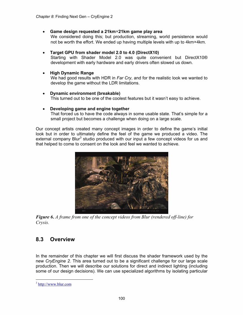
Our concept artists created many concept images in order to define the game’s initial look but in order to ultimately define the feel of the game we produced a video. The external company Blur3 studio produced with our input a few concept videos for us and that helped to come to consent on the look and feel we wanted to achieve.

Figure 6. A frame from one of the concept videos from Blur (rendered off-line) for Crysis. 8.3 Overview In the remainder of this chapter we will first discuss the shader framework used by the new CryEngine 2. This area turned out to be a significant challenge for our large scale production. Then we will describe our solutions for direct and indirect lighting (including some of our design decisions). We can use specialized algorithms by isolating particular

3 http://www.blur.com


101

lighting approach into a contained problem and solving it in the most efficient way. In that context, we approach direct lighting primarily from the point of view of shadowing (since shading can be done quite easily with shaders of varied sophistication). Indirect lighting can be approximated by ambient occlusion, a simple darkening of the ambient shading contribution. Finally we cover various algorithms that solve the level of detail problem. Of course this chapter will only cover but a few rendering aspects of our engine and many topics will be left uncovered – but it should give a good “taste” of the complexity of our system and allow us to dig in into a few select areas in sufficient details. 8.4 Shaders and Shading

8.4.1 Historical Perspective on CryEngine 1 In Far Cry we supported graphics hardware down to NVIDIA GeForce 2 which means we not only had pixel and vertex shader but also fixed function transform and lighting (T&L) and register combiner (pre pixel shader solution to blend textures) support. Because of that and to support complex materials for DirectX and OpenGL our shader scripts had complex syntax. After Far Cry we wanted to improve that and refactored the system. We removed fixed function support and made the syntax more FX-like as described in [Microsoft07]. Very late in the project our renderer programmer introduced a new render path that was based on some über-shader approach. That was basically one pixel shader and vertex shader written in CG/HLSL with a lot of #ifdef. That turned out to be much simpler and faster for development as we completely avoided the hand optimization step. The early shader compilers were not always able to create shaders as optimal as humans could do but it was a good solution for shader model 2.0 graphics cards. The über-shader had so many variations that compiling all of them was simply not possible. We accepted a noticeable stall due to compilation during development (when shader compilation was necessary) but we wanted to ship the game with a shader cache that had all shaders precompiled. We ended up playing the game on NVIDIA and on ATI till the cache wasn’t getting new entries. We shipped Far Cry with that but clearly that wasn’t a good solution and we had to improve that. We describe a lot more details about our first engine in [Wenzel05].

8.4.2 CryEngine 2 We decided to reduce a number of requirements for cleaner engine. As a result we removed support for OpenGL and fixed function pipeline support. This allowed us to make the shader scripts more FX format compatible. Then developing shaders became much more convenient and simple to learn.


102

We still had the problem with too many shader combinations and wanted to solve that. We changed the system by creating a shader cache request list. That list was gathered from all computers in the company over the network and it was used during the nightly shader cache compilation. However compilation time was long so we constantly had to reduce the amount of combinations. We had the following options:

x Dynamic branching x Reducing combinations and accepting less functionality

x Reducing combinations and accepting less performance

x Separating into multiple passes

We did that in multiple iterations and together with a distributed shader compilation we managed to compile all shaders for a build in about an hour.

8.4.3 3DcTM for Normal Maps The 3DcTM texture format introduced by ATI [ATI04] allows compressing normal maps in one byte per texel with good quality and only little extra shader cost (reconstructing the z component). Uncompressed normal maps cost 4 bytes per texel (XYZ stored in RGB, one byte usually wasted for padding). In our new engine we decided to not do texture compression at load time. Textures become processed by our resource compiler tool and there we generate the mip levels and apply the compression. This way we get smaller builds and faster loading. For hardware that doesn’t allow 3DcTM compression we convert the 3DcTM to DXT5 at load time. The formats are quite similar and conversion is simple. The minor quality loss is acceptable for low spec. Older NVIDIA cards have 3DcTM emulation in the drivers so we don’t have to take care of that (appears without visible quality loss, however, with this solution requires 2 byte per texel storage).

8.4.4 Per-Pixel Scene Depth Using an early z pass can reduce per pixel shading cost because many pixel can be rejected based on the z value before a pixel shader needs to be executed. From beginning on we based our rendering on early z because we expected heavy pixel shader usage. For that we have to accept a higher draw call count. For many effects the depth value would be useful. As it wasn’t possible to bind the z buffer we decided to output that value to a texture. At first we used the R16G16 texture format as this was available on all hardware and the 16 bit float quality was sufficient. Initially we had some use for the second channel but later we optimized that away. On ATI R16 was an option and to save some memory and bandwidth we used that format. We realized on some hardware the R16G16 is actually slower than the R32 format so we used R32 when R16 was not available. An even better option is using the z buffer directly as we don’t need


103

extra memory and the early z pass can run faster (double speed without color write on some hardware). So we ended up using R16, R32 or even native z buffer – depending on what is available. The depth value allows some tricks known from deferred shading. With one MAD operation and a 3 component interpolator it’s possible to reconstruct the world space position. However for floating point precision it’s better to reconstruct positions relative to the camera position or some point near to it. That is especially important when using 24bit or 16bit float in the pixel shader. By offsetting all objects and lights it’s possible move the 0, 0, 0 origin near the viewer. Without doing this decals and animations can flicker and jump. We used the scene depth for per pixel atmospheric effects like the global fog, fog volumes and soft z buffered particles. Shadow mask generation uses scene depth to reduce draw call count. For the water we use the depth value to soft clip the water and fade in a procedural shore effect. Several post processing effects like motion blur, Depth of Field and Edge blurring (EdgeAA) make use of the per pixel depth as well. We describe these effects in detail in [Wenzel07].

8.4.5 World Space Shading In Far Cry we transformed the view and the light positions into tangent space (relative to the surface orientation). All data in the pixel shader was in tangent space so shading computations were done in that space. With multiple lights we were running into problems passing the light parameters over the limited amount of interpolators. To overcome this problem we switched to use world-space shading for all computations in Crisis (in actuality we use world-space shading with an offset in order to reduce floating point precision issues). The method was already needed for cube map reflections so code became more unified and shading quality improved as this space is not distorted as tangent space can be. Parameters like light position now can be passed in pixel shader constants and don’t need to be updated for each object. However when using only one light and simple shading the extra pixel cost is higher. 8.5 Shadows and Ambient Occlusion

8.5.1 Shadowing Approach in CryEngine 1 In our first title Far Cry we had shadow maps and projected shadows per object for the sun shadows. We suffered from typical shadow map aliasing quality issues but it was a good choice at that time. For performance reasons we pre-computed vegetation shadows but memory restrictions limited us to very blurry textures. For high end


104

hardware configurations we added shadow maps even to vegetation but combining them with the pre-computed solution was flawed. We used stencil shadows for point lights as that were an easier and more efficient solution. CPU skinning allowed shadow silhouette extraction on the CPU and the GPU rendered the stencil shadows. It became obvious that this technique would become a problem the more detailed objects we wanted to render. It relied on CPU skinning, required extra CPU computation, an upload to GPU, extra memory for the edge data structures and had hardly predictable performance characteristics. The missing support for alpha-blended or tested shadow casters made this technique not even usable for the palm trees – an asset that was crucial for the tropical island look (Figure 7).

Figure 7. Far Cry screenshot: note how the soft precomputed shadows combine with the real-time shadows For some time during development we had hoped the stencil shadows could be used for all indoor shadows. However the hard stencil shadows look and performance issues with many lights made us search for other solutions as well. One of such solutions is to rely on light maps for shadowing. Light maps have the same performance no matter how many lights and allow a soft penumbra. Unfortunately what is usually stored is the result of the shading, a simple RGB color. That doesn’t allow normal mapping. We managed to solve this problem and named our solution Dot3Lightmaps [Mittring04]. In this approach the light map stores an average light direction in tangent space together with an average light color and a blend value to lerp between pure ambient and pure directional lighting. That allowed us to render the diffuse contribution of static lights with soft shadows quite efficiently. However it was hard to combine with real-time shadows. After Far Cry we experimented with a simple modification that we named Occlusion maps. The main concept is to store the shadow mask value, a scalar value from 0 to 1 that represents the percentage of geometry occlusion for a texel. We stored the shadow mask of multiple lights in the light map texture and the usual four texture channels allowed four lights per texel. This way we rendered diffuse and specular contributions of static lights with high quality soft shadows while the light color and strength remained adjustable. We kept lights separate so combining with other shadow types was possible.


105

8.5.2 The Plan for CryEngine 2 The time seemed right for a clean unified shadow system. Because of the problems mentioned we decided to drop stencil shadows. Shadow maps offer high quality soft shadows and can be adjusted for better performance or quality so that was our choice. However that only covers the direct lighting and without the indirect lighting component the image would not get the cinematographic realistic look we wanted to achieve. The plan was to have a specialized solution for the direct and another one for the indirect lighting component.

8.5.3 Direct Lighting For direct lighting we decided to apply shadow maps (storing depth of objects seen from the light in a 2D texture) only and drop all stencil shadow code.

8.5.3.1 Dynamic Occlusion Maps To efficiently handle static lighting situations we wanted to do something new. By using some kind of unique unwrapping of the indoor geometry the shadow map lookup results could be stored into an occlusion map and dynamically updated. The dynamic occlusion map idea was good and it worked but shadows often showed aliasing as now we not only had shadow map aliasing but also unwrapping aliasing. Stretched textures introduced more artifacts and it was hard to get rid of all the seams. Additionally we still required shadow maps for dynamic objects so we decided to get the maximum out of normal shadow maps and dropped the caching in occlusions maps.

8.5.3.2 Shadow Maps with Screen-Space Randomized Look-up Plain shadow mapping suffers from aliasing and has hard jagged edges (see first image in Figure ). The PCF extension (percentage closer filtering) limits the problem (second image in Figure ) but it requires many samples. Additionally at the time hardware support was only available on NVIDIA graphics cards such as GeForce 6 and 7 generation and emulation was even slower. We could implement the same approach on newer ATI graphics cards by using Fetch4 functionality (as described in [Isidoro06]). Instead of adding more samples to the PCF filter we had the idea to randomize the lookup per pixel so that less samples result in similar quality accepting a bit of image noise. Noise (or grain) is part of any film image and the sample count offers an ideal property to adjust between quality and performance. The idea was inspired by soft shadow algorithms for ray tracing and already applied to shadow maps on GPU (See [Uralsky05] and [Isidoro06] for many details with regards to shadow map quality improvement and optimization).


106

The randomized offsets that form a disk shape can be applied in 2D when doing the texture lookup. When using big offsets the quality for flat surfaces can be improved by orienting the disk shape to the surface. Using a 3D shape like a sphere can have higher shading cost but it might soften bias problems. To get acceptable results without too much noise multiple samples are needed. The sample count and the randomization algorithm can be chosen depending on quality and performance needs. We tried two main approaches: randomly rotated static kernel [Isidoro06] and another technique that allowed a simpler pixel shader.

Figure 8. Example of shadow mapping with varied resulting quality: from left to right: no PCF, PCF, 8 samples, 8 samples+blur, PCF+8 samples, PCF+8 samples+blur The first technique requires a static table of random 2D points and a texture with random rotation matrices. Luckily the rotation matrixes are small (2×2) and can be efficiently stored in a 4 component texture. As the matrices are orthogonal further compression is possible but not required. Negative numbers can be represented by the usual “scale and bias” trick (multiply the value by 2 and subtract 1) or by using floating point textures. We tried different sample tables and in the Figure 8 you can see an example of applying this approach to a soft disc that works quite well. For a disc shaped caster you would expect a filled disk but we haven’t added the inner samples as the random rotation of those are less useful for sampling. The effect is rarely visible but to get more correct results we still consider changing it. The simpler technique finds its sample positions by transforming one or two random positive 2D positions from the texture with simple transformations. The first point can be placed in the middle (mx, my) and four other points can be placed around using the random value (x, y).

(mx, my) (mx+x, my+y) (mx-y, my+x) (mx-x, my-y) (mx+y, my-x)

More points can be constructed accordingly but we found it only useful for materials rendered on low end hardware configurations (where we would want to keep the sample count low for performance reasons).


107

Both techniques also allow adjusting the kernel size to simulate soft shadows. To get proper results this kernel adjustment would be dependent on the caster distance and the light radius but often this can be approximated much easier. Initially we randomized by using a 64x64 texture tiled with a 1:1 pixel mapping over the screen (Figure 9)

Figure 9. An example of the randomized kernel adjustment texture

This texture (Figure 9) was carefully crafted to appear random without recognizable features and with most details in the higher frequencies. Creating a random texture is fairly straight-forward; we can manually reject textures with recognizable features and we can maximize higher frequencies applying a simple algorithm that finds a good pair of neighbor pixels that can be swapped. A good swapping pair will increase high frequencies (computed by summing up the differences). While there are certainly better methods to create a random texture with high frequencies), we only describe but this simple technique as it served our purposes. Film grain effect is not a static effect so we could potentially animate the noise and expect it to hide low sample count even more. Unfortunately the result was perceived as a new type of artifact with low or varying frame rate. Noise without animation looked pleasing for static scenes; however with a moving camera some recognizable static features in the random noise remained on the screen.

8.5.3.3 Shadow Maps with Light-Space Randomized Look-up Fortunately we found a good solution for that problem. Instead of projecting the noise to the screen we projected a mip-mapped noise texture in world space in the light/sun direction. In medium and far distance the result was the same but because of bilinear magnification the nearby shadow edges became distorted and no longer noisy. That looked significantly better – particularly for foliage and vegetation, where the exact shadow shape was hard to determine.

8.5.3.4 Shadow Mask Texture We separated the shadow lookup from shading in our shaders in order to avoid the instruction count limitations of Shader Model 2.0, as well as to reduce the number of resulting shader combinations and be able to combine multiple shadows. We stored the 8 bit result of the shadow map lookup in a screen-space texture we named shadow


108

mask. The 4 channel 32 bit texture format offers the required bit count and it can be used as a render target. As we have 4 channels we can combine up to 4 light contributions in a texel.

Figure 10. Example of shadow maps with randomized look-up. Left top row image: no jittering 1 sample, right top row image: screen space noise 8 samples, left bottom: world space noise 8 samples, right bottom: world space noise with tweaked settings 8 samples


109

Figure 11. Example of the shadow mask texture for a given scene: Left: final rendering with sun (as a shadow caster) and two shadow-casting lights, right: light mask texture with three lights in the RGB channels

Figure 12. Example of the shadow mask texture for a given scene - Red, Green and Blue channel store the shadow mask for 3 individual lights In the shading pass we bind this texture and render multiple lights and the ambient at once. We could have used the alpha channel of the frame buffer but then we would have more passes and draw call count would raise a lot. For opaque objects and alpha test surfaces the shadow mask is a good solution but it doesn’t work very well for alpha blended geometry. All opaque geometry is represented in the depth buffer but alpha blended geometry is not modifying the depth buffer. Transparent geometry requires normal shadow map lookup in the shader.

8.5.3.5 Shadow Maps for Directional Light Sources In Far Cry we had only a few shadow casting objects and each had its own shadow map. For many objects its better to combine them on one shadow map. A simple parallel projection in the direction of the light works but near the viewer the shadow map resolution is quite low and then shadows appear blocky. Changing the parameterization like finding a projection matrix that moved more resolution near the viewer is possible but not without problems. We tried trapezoidal shadow maps ([MT04]) (TSM) and perspective shadow maps ([SD02]) (PSM). We had more success with cascaded shadow maps (CSM) where multiple shadow maps of the same resolution cover the viewer area with multiple projections. Each projection is enclosed by the previous one with decreasing world to texel ratio. That technique was giving satisfactory results but wasted some texture space. That was because the projection only roughly concentrated to the area in front of the viewer. To find proper projection the view frustum (reduced by the shadow receiving distance) can


110

be sliced up. Each shadow map needs to covers one slice. Slices farther away can cover bigger world space areas. If the shadow map projection covers the slices tightly then minimal shadow map area is wasted. With earlier shadow techniques we already had aliasing of the shadow maps when doing camera movements and rotations. For PSM and TSM we haven’t been able to solve the issue but for CSM and its modification it was possible. We simply snapped the projections per shadow map texel and that resulted in a much cleaner look.

8.5.3.6 Deferred Shadow Mask Generation The initial shadow mask generation pass required rendering of all receiving objects and that resulted in many draw calls. We decoupled shadow mask generation from the receiver object count by using deferred techniques. We basically render a full screen pass that binds the depth texture we created in the early z pass. Simple pixel shader computations give us the shadow map lookup position based on the depth value. The indirection over the world-space position is not needed. As mentioned before we used multiple shadow maps so the shadow mask generation pixel shader had to identify for each pixel in which shadow map it falls and index into the right texture. Indexing into a texture can be done with DirectX10 texture arrays feature or by offsetting the lookup within a combined texture. By using the stencil buffer we were able to separate processing of the individual slices and that simplified the pixel shader. Indexing was not needed any more. The modified technique runs faster as less complex pixel shader computations need to be done. It also carves away far distant areas that don’t receive shadows.

8.5.3.7 Unwrapped Shadow Maps for Point Lights The usual shadow map approach for point light sources require a cube map texture lookup. But then hardware PCF cannot be used and on cube maps there is much less control for managing the texture memory. We unwrapped the cube map into six shadow maps by separating the six cases with the stencil buffer, similar we did for CSM. This way we transformed the point light source problem to the projector light problem. That unified the code and resulted in less code to maintain and optimize and less shader combinations.

8.5.3.8 Variance Shadow Maps For terrain we initially wanted to pre-compute a texture with start and end angle. We also tried to update an occlusion map in real-time with incremental updates. However the


111

problem has always been objects on the terrain. Big objects, partly on different terrain sectors required proper shadows. We tried to use our normal shadow map approach and it gave us a consistent look that wasn’t soft enough. Simply making the randomized lookup with a bigger radius would be far too noisy. Here we tried variance shadow maps [DL06] and this approach has worked out nicely. The usual drawback of variance shadow maps arises with multiple shadow casters behind each other but that’s a rare case with terrain shadows.

Figure 13. Example of applying variance shadow maps to a scene. Top image: variance shadow maps aren’t used (note the hard normal shadows), bottom image: with variance shadow maps (note how the two shadow types combine)

8.5.4 Indirect Lighting The indirect lighting solution can be split in two sub-problems: the processing intensive part of computing the indirect lighting and the reconstruction of the data in the pixel shader (to support per-pixel lighting).

8.5.4.1 3D Transport Sampler For the first part we had planned to develop a tool called 3D transport sampler. This tool would make it possible to compute the global illumination data distributed on multiple machines (for performance reasons). Photon mapping ([Jensen01]) is one of the most accepted methods for global illumination computation. We decided to use this method because it can be easily integrated and delivers good results quickly. The photon


112

Figure 14. Real-time ambient maps with one light source mapper was first used to create a simple light map. The unwrapping technique in our old light mapper was simple and only combined triangles that were connected and had a similar plane equation. That resulted in many small 2D blocks we packed into multiple textures. When used for detailed models it became inefficient in texture usage and it resulted in many small discontinuities on the unwrapping borders. We changed the unwrapping technique so it uses the models UV unwrapping as a base and modifies the unwrapping only where needed. This way the artist had more control over the process and the technique is more suitable for detailed models. We considered storing Dot3Lightmaps (explained earlier) but what we tried was a method that should result in better quality. The idea was to store light contributions for four directions oriented to the surface. This is similar to the technique that was used in Half-Life 2 ([McTaggart04]) but there only three directions were used. The more data would allow better quality shading. The data would allow high quality per-pixel lighting and accepting some approximations it could be combined with real-time shadows. However storage cost was huge and computation time was high so we aborted this approach. Actually our original plan was to store some light map coefficients per texel and others per vertex. Together with a graph data structure that is connected to the vertices it should be possible to get dynamic indirect lighting. Low frequency components of the indirect lighting could be stored in the vertices and high frequency components like sharp corners could be stored per texel. Development time was critical so this idea was dropped.

8.5.4.2 Real-Time Ambient Map (RAM) As an alternative we chose a much simpler solution which only required storing one scalar ambient occlusion value per texel. Ambient occlusion ([ZIK98, Landis02]) can be computed by shooting rays in all directions – something that was reusable from the photon mapper. The reconstruction in the shader was using what was available: the


113

texel with the occlusion value, the light position relative to the surface, the light color and the surface normal. The result was a crude approximation of indirect lighting but the human eye is very forgiving for indirect lighting so it worked out very well. To support normal maps some average light direction is needed and because of the lack of something better the light direction blended with the surface normal was used. This way the normal maps still can be seen and shading appear to have some light angle dependency. Having ambient brightness, color and attenuation curve adjustable allowed designers to tweak the final look. The technique was greater extended to take portals into account, to combine multiple lights and to support the sun. For huge outdoor areas computing the RAM data for every surface wouldn’t be feasible so we approached that differently.

8.5.4.3 Screen-Space Ambient Occlusion One of our creative programmers had the idea to use the z buffer data we already had in a texture to compute some kind of ambient occlusion. The idea was tempting because all opaque objects could be handled without special cases in constant time and constant memory. We also could remove a lot of complexity in many areas. Our existing solutions worked but it we had issues to handle all kind of dynamic situations. The approach was based on sampling the surrounding of a pixel and with some simple depth comparisons it was possible to compute a darkening factor to get silhouettes around objects. To get the ambient occlusion look this effect was limited to only nearby receivers. After several iterations and optimizations we finally had an unexpected new feature and we called it “Screen-Space Ambient Occlusion” (SSAO). We compute the screen-space ambient occlusion in a full screen pass. We experimented by applying it on ambient, diffuse and specular shading but we found it works best on ambient only. That was mostly because it changed the look away from being realistic and that was one of our goals. To reduce the sample count we vary the sample position for nearby pixels. The initial sample positions are distributed around the origin in a sphere and the variation is achieved by reflecting the sample positions on a random 3D plane through the origin. n: the normalized random per pixel vector from the texture

i: one of the 3D sample positions in a sphere

float3 reflect( float3 i, float3 n ) { return i - 2 * dot(i, n) * n; The reflection is simple to compute and it’s enough to store the normalized plane normal in a texture.


114

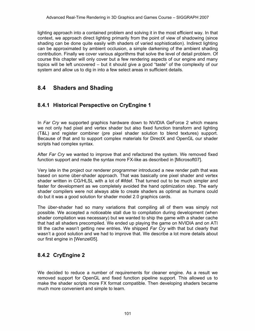
Figure 15. Screen-Space Ambient Occlusion in a complete ambient lighting situation (note how occluded areas darken at any distance)

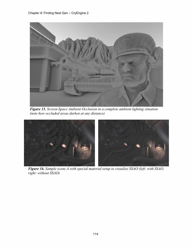
Figure 16. Sample scene A with special material setup to visualize SSAO (left: with SSAO, right: without SSAO)


115

Figure 17. Sample scene B with special material setup to visualize SSAO (left: with SSAO, right: without SSAO)

Figure 18. Sample scene A with special material setup to visualize SSAO (left: with SSAO, right: without SSAO) 8.6 Level of Detail

8.6.1 Situation Level of Detail (LOD) is especially important if the rendering complexity cannot be easily restricted. Most games have either quite limited view range often realized with fog or strong occlusion set up by level designers. That’s why many games are dominated by indoor environments but in Far Cry we wanted to show big landscapes with many details without restricting the players view or position. In Crysis we kept the view range but added more objects with more variety and higher quality. Quality means more complex pixel and vertex shaders, higher resolution textures, new texture types (e.g. subsurface) and more vertices. As we additionally decided to use an early z pass and real-time shadows we have to pay an even higher price for each object. Because of the higher draw call count this is mainly a CPU burden and that is one of the areas where DirectX10 is better. In Far Cry we simply switched between artist-created LOD models. We also used impostors for vegetation and improved them for Crysis but that’s beyond the scope this chapter.


116

In Crysis we considered using a smooth LOD transition based on moving vertices. Such techniques often introduce many restrictions for the asset creation. Without such restrictions assets often can be more optimal and created more quickly. That is especially true for vegetation rendered alpha-tested or alpha-blended. For some time we had no transition between LODs and for demo purposes we disabled lower LOD levels completely. Demo machines have high spec hardware and there the smaller LOD levels had no increased effect. Lower LODs are usually small on the screen so per pixel cost is low. Having many LOD levels can be even counterproductive, as those cannot be instanced together and, so we suffer from higher draw call count.

8.6.2 Dissolve One of our programmers finally had the idea of a soft LOD transition based on dissolving the object in the early z pass. As we later on render with z equal comparison we only had to adjust the early z pass. That was not completely true as surfaces can have exactly the same z value and then with additive blending those pixels would become twice as bright. However as the first rendering pass of each object has frame buffer blending disabled the problem should only occur with subsequent passes. As we can combine multiple lights in one pass this is a rare case anyway. The dissolve texture is projected in screen space, and by combining the random value from the texture with a per object transition value, the pixels are rejected with the texkill operation or simple alpha-test. With the Alpha2Coverage feature and full scene anti-aliasing (FSAA) of modern cards that can be even done on a sub-pixel level. Even without FSAA the dissolve is not that noticeable if we enable our edge-blurring post processing effect. Initially we had the transition state only depend on object distance but objects that are in transition are slower to render and for quality reasons it’s better to hide it. That’s why we added code to finish started transitions within a defined small amount of time. We not only use the dissolve for transitions between 3D objects but also to fade out far away objects and to hide the transition to impostors.

8.6.3 Water Surface LOD The ocean or big water surfaces in general have some unique properties that can be used by specialized render algorithms. Our initial implementation that we used in Far Cry was based on a simple disk mesh that moved around with the player. Pixel shading, reflections and transparency defined the look. However we wanted to have real 3D waves, not based on physical simulation but a cheap procedural solution. We experimented with some FFT based ocean waves simulation ([Jensen01a], [Tessendorf04]). To get 3D waves vertex position manipulation was required and the mesh we used so far wasn’t serving that purpose.


117

8.6.4 Square Water Sectors The FFT mentioned earlier only outputs a small sector of the ocean and to get a surface till the horizon we rendered the mesh multiple times. Different LODs had different index buffers but they all referenced to one vertex buffer that had the FFT data. We shared the vertex buffer to save performance but for better quality down sampling would be needed. To reduce aliasing artifacts in the distance and to limit the low polygonal look in the near we faded out the perturbation for distant vertices and limited the perturbation in the near. The algorithm worked but many artifacts made us search for a better solution.

8.6.5 Screen-Space Tessellation We tried a brute force approach that was surprisingly simple and worked out very well. We used a precomputed screen space tessellated quad and projected the whole mesh onto the water surface. This ensures correct z buffer behavior and even clips away pixels above the horizon line. To modify the vertex positions with the FFT wave simulation data we require vertex texture lookup so this feature cannot be used on all hardware.

Figure 2. Screen-space tessellation in wireframe

The visible vertical lines in the wireframe are due to the mesh stripification we do for better vertex cache performance. The results looked quite promising however vertices on the screen border often moved farther away from the border and that was unacceptable. Adding more vertices even outside of the screen would solve the problem but attenuating the perturbations on the screen border are hardly noticeable and have only minimal extra cost.


118

Figure 3. Left: screen space tessellation without edge attenuation (note the area on the left not covered by water), right: screen space tessellation with edge attenuation For better performance we reduced the mesh tessellation. Artifacts remained acceptable even with far less vertices. Tilting the camera made it a slightly worse but not as much as we expected. The edge attenuation made the water surface camera dependent and that was bad for proper physics interaction. We had to reduce the wave amplitude a lot to limit the problem.

8.6.6 Camera Aligned The remaining issues aliasing artifacts and physics interaction bothered our shader programmer and he spent some extra hours finding a solution for this. This new method used a static mesh like the one before. The mesh projection changed from a perspective to a simple top down projection. The mesh is dragged around with the camera and the offset is adjusted to get most of the mesh in front of the camera. To render up to the horizon line the mesh borders are expanded significantly. Tessellation in that area is not crucial as perturbation can be faded to 0 before that distance.

Figure 204. Camera aligned water mesh in wire frame. Left: camera aligned from top down, right: camera aligned from viewer perspective The results of this method are superior to the screen space ones which becomes mostly visible in motion with subtle camera movement. Apart from the distance attenuation the wave extent is now viewer independent and as the FFT data is CPU accessible physics interactions are now possible.


119

Figure 21. Left: Camera aligned, right: screen space tessellation as comparison 8.6 Conclusion Through some intricate path we not only found our next generation engine but we also learned a lot. That learning process was necessary to find, validate and compare different solutions so in retro perspective it can be classified to research. Why we chose certain solutions in favor of others is mostly because of quality, production time, performance and scalability. Crysis, our current game, is a big scale production and to handle this the production time is very important. Performance of a solution is hardware dependent (e.g. CPU, GPU, memory) so on a different platform we might have to reconsider. The current engine is streamlined for a fast DirectX9/DirectX10 card with one or multiple CPU cores. Having the depth from the early z pass turned out to be very useful; many features now rely on this functionality. Regular deferred shading also stores more information per pixel like the diffuse color, normal and other material properties. For the alien indoor environment that would probably be the best solution but other environments would suffer from that decision. In a one light source situation deferred shading simply cannot play out its advantages. 8.6 Acknowledgements This presentation is based on the passionate work of many programmers, artist and designers. Special thanks I would like to contribute to Vladimir Kajalin, Andrey Khonich, Tiago Sousa, Carsten Wenzel and Nick Kasyan. Because we have been launch partners with NVIDIA we had on-site help not only for G80 DirectX9 and DirectX10 issues. Special thanks to those NVIDIA engineers namely Miguel Sainz, Yury Uralsky and Philip Gerasimov. Leading companies of the industry Microsoft, AMD, Intel and NVIDIA and many others have been very supportive. Additional thanks to Natalya Tatarchuk and Tim Parlett that helped me to get this done.


120

8.7 References [ATI04] ATI 2004, Radeon X800 3DcTM Whitepaper

http://ati.de/products/radeonx800/3DcWhitePaper.pdf

[DL06] DONNELLY W. AND LAURITZEN A. 2006. Variance shadow maps. In Proceedings of the 2006 ACM SIGGRAPH Symposium on Interactive 3D graphics and games, pp. 161-165. Redwood City, CA

[ISIDORO06] ISIDORO J. 2006. Shadow Mapping: GPU-based Tips and Techniques. GDC

presentation. http://ati.amd.com/developer/gdc/2006/Isidoro-ShadowMapping.pdf [JENSEN01] JENSEN, H. W. 2001. Realistic image synthesis using photon mapping, A. K. Peters, Ltd., Natick, MA. [JENSEN01a] JENSEN, L. 2001, Deep-Water Animation and Rendering, Gamasutra article

http://www.gamasutra.com/gdce/2001/jensen/jensen_pfv.htm [LANDIS02] LANDIS, H., 2002. RenderMan in Production, ACM SIGGRAPH 2002 Course

16. [MICROSOFT07] MICROSOFT DIRECTX SDK. April 2007. http://www.microsoft.com/downloads/details.aspx?FamilyID=86cf7fa2-e953-475c-

abde-f016e4f7b61a&DisplayLang=en [MT04] MARTIN, T. AND TAN, T.-S. 2004. Anti-aliasing and continuity with trapezoidal

shadow maps. In proceedings of Eurographics Symposium on Rendering 2004, pp. 153–160, 2004.

[MCTAGGART04] MCTAGGART, G. 2004. Half-Life 2 Shading, GDC Direct3D Tutorial http://www2.ati.com/developer/gdc/D3DTutorial10_Half-Life2_Shading.pdf [MITTRING04] MITTRING, M. 2004. Method and Computer Program Product for Lighting a

Computer Graphics Image and a Computer. US Patent 2004/0155879 A1, August 12, 2004.

[SD02] STAMMINGER, M. AND DRETTAKIS, G. 2002. Perspective shadow maps. In

SIGGRAPH 2002 Conference Proceedings, volume 21, 3, pages 557–562, July 2002 [TESSENDORF04] TESSENDORF, J. 2004. Simulating Ocean Surfaces. Part of ACM

SIGGRAPH 2004 Course 32, The Elements of Nature: Interactive and Realistic Techniques, Los Angeles, CA

[URALSKY05] URALSKY, Y. 2005. Efficient Soft-Edged Shadows Using Pixel Shader

Branching. In GPU Gems 2, M. Pharr, Ed., Addison-Wesley, pp. 269 – 282. [WENZEL05] WENZEL C. 2005. Far Cry and DirectX. GDC presentation, San Francisco, CA http://ati.amd.com/developer/gdc/D3DTutorial08_FarCryAndDX9.pdf


121

[WENZEL06] WENZEL, C. 2006. Real-time Atmospheric Effects in Games. Course 26: Advanced Real-Time Rendering in 3D Graphics and Games. Siggraph, Boston, MA. August 2006

http://ati.amd.com/developer/techreports/2006/SIGGRAPH2006/Course_26_SIGGRAPH_2006.pdf

[WENZEL07] WENZEL C. 2007. Real-time Atmospheric Effects in Games Revisited.

Conference Session. GDC 2007. March 5-9, 2007, San Francisco, CA. http://ati.amd.com/developer/gdc/2007/D3DTutorial_Crytek.pdf

[ZIK98] ZHUKOV, S., IONES, A., AND KRONIN, G. 1998. An ambient light illumination model.

In Rendering Techniques ’98 (Proceedings of the Eurographics Workshop on Rendering), pp. 45–55.

finding next gen – cryengine 2 - home - amd · finding next gen – cryengine 2 martin mittring14...

Documents