FINAL REPORT

NASA CONTRACT NAS8-39716

TEMPERATURE DEPENDENCE OF DIFFUSIVITIES

IN LIQUID ELEMENTS (LMD)

Period of Performance

2/3/93 through 5/31/98

Principle Investigators

R. MICHAEL BANISH

FRANZ ROSENBERGER (Retired)

Center for Microgravity and Materials ResearchUniversity of Alabama in Huntsville

Huntsville, Alabama 35899

https://ntrs.nasa.gov/search.jsp?R=19990106564 2018-06-07T23:59:44+00:00Z

Table of Contents

Introduction .................................................................................................................... 1

1Background ............................................................................................................

2Objectives and Tasks ..............................................................................................

Work Performed under this Contract ............................................................................ 2

Measurement Methodology .............................................................................. 2Early methodology investigations ......................................................... 3Codastefano methodology ...................................................................... 4

Hardware Design and Construction ................................................................... 5Choice of radiation dtectors .................................................................. 5

Diffusion sample and Ampoule ............................................................. 6Isothermal liner/radiation shield ........................................................... 8

Choice of Isotopes to be Used ........................................................................... 8Class-like self-diffusion behavior of molten elements ......................... 9

High/low energy photons for wall effect investigations ........................ 10Systems to be used in diffusivity measurements .................................. 10

Convective Effects on Diffusivity Measurements ............................ -............... 11Numerical modelling of magnetic fields to suppress convecuon ......... 11Numerical modelling of bouyancy-driven convection ........................... 14

Risk Mitigation Flight Opportunity ................................................................... 15Application of the technique to indium ................................................. 16

References ..................................................................................................................... 20

Publications and Invited Presentations ......................................................................... 22

AppendicesReal-time Diffusivity Measurements in Liquids at Several Temperature

with one Sample ..............................................................................................

On the Sensitivity of Liquid Diffusivity Measurements to Deviationsfrom 1-D Diffusion ..........................................................................................

Numerical simulations of the convective contamination of diffusivity

measurements in liquids .................................................................................

23

34

41

INTROD UCTION

This report is a summary of the work performed under NASA grant NAS8-39716 (Liquid

Metal Diffusion). This research was to advance the understanding of diffusion mechanisms in

liquid metals and alloys through accurate diffusivity measurements over a wide range of

temperatures, including the proximity of the materials melting points. Specifically, it was driven

towards developing a methodology (and subsequent flight hardware) to enable several diffusion

coefficient measurements (i.e., at several different temperatures) to be performed using a single

sample.

The Liquid Metal Diffusion (LMD) was funded as a Flight Definition Project in February 1993

in response to NRA 91-OSSA-20 (Microgravity Science and Applications Division). The Science

Concept Review for LMD was held during April 1994. In January 1995 we were informed that

we had failed this review and the project was change to ground-based activities only. A new

proposal was submitted for the next NRA addressing the panels concerns.

As part of NASA's Risk Mitigation program, a scaled-down version of the hardware was

funded in July of 1995 for a flight opportunity utilizing experiment on the Microgravity Isolation

Mount. This experiment was to determine the self-diffusivity of indium at 185°C. The LMD was

transferred to the Mir Space Station in STS-81 and returned on STS-84 (January - May 1997).

Three, out of five, self-diffusion data sets were returned. A description of this

experiment/hardware is included below.

This summary is only intended to give the reader an overview of the results obtained for the

tasks outlined in the original proposal. Research that was not published is explained in more

detail. At the end of this report is a list of refereed publications and invited talks that were given asa result of this work. The reader is directed to these for further details.

Background

The diffusion of species in liquids governs numerous materials preparation processes of

technological importance. In particular, a detailed understanding of diffusion in liquid metals and

alloys is pivotal for the interpretation of various phenomena encountered in metallurgical and

semiconductor manufacturing processes. Transport experiments in gases and crystalline solids can

readily be designed to yield diffusion coefficients with great accuracy at normal gravity [1]. In

liquids, however, such measurements are hampered by uncontrollable and significant contributionsfrom convection.

Simple scaling illustrates the difficulty of obtaining purely diffusive transport in liquids: In a

system with a diffusivity of 10 -5 cm2/s and a characteristic diffusion distance of about 1 cm, the

diffusion velocity is of the order of 10 -5 cm/s. If true diffusion is to be observed, convective

contributions to mass transport must be small compared to the diffusion fluxes. Therefore,

convection velocities parallel to the concentration gradient must be of order 10 .7 cm/s (10 ,/k/sec !)

or less. Hence, the results of diffusion experiments in liquids tend to be contaminated by

buoyancy-driven flows.

As a consequence, the standard deviations of liquid diffusivity data obtained on Earth range

typically from several 10% to several 100% [2]. This high uncertainty is particularly deplorable

since, due to the complex structures of liquids and, thus, the lack of realistic structure models, our

theoretical understanding of diffusion in liquids is very limited. There are currently various

theoreticalmodelsfor thetemperaturedependenceof diffusivitiesin liquids. The predictionsrangefrom apureArrhenius-typebehavior (exponentialincreasewith temperature)to combinationsofArrheniuslawswith powerlaws andpurepower laws [2,3]. However,due to thelargescatterofexistingliquid diffusivity data,it is currentlynot possibleto adequatelyevaluatethesetheories.Thus, accurateliquid diffusion dataareneededto provideguidancein the developmentof bothfundamentaldiffusiontheoryandtransportmodelsessentialfor materialsprocessing.

Efforts to excludeconvectivetransportcontributionsin diffusionexperimentsby usingnarrowcapillarieshaverevealedcontaminationof theresultsby (poorly understood)wall effects[4, andreferencesin 2]. It appearsasif, in analogyto surfaceandinterfacediffusion in solids, dependingon thematerialsinvolved, lower or higherdiffusion fluxes exist in a thin layer at the containerwall. This effectsetslower limits to theusefulcapillarydiameter.Thus, thedrasticreductionofbuoyancy-drivenconvectionunderlow gravityconditionsprovidesapromisingmeansof studyingtruediffusion in liquids.

Objectives and Tasks

Within this framework the following technological and scientific objectives were proposed:

• Development of a technique for dynamic in-situ measurements of diffusivities and their

temperature dependence in melts, with much higher efficiency than current (one sample/one

data point) approaches permit.

• Development of a flight-certified hardware package (GAS container) to perform such

diffusivity measurements automatically, with relatively high flight frequency.

• Establishment of a large definitive database for the temperature dependence of self-diffusivities

in liquid metals and alloys, in order to further the development of the theory of diffusion in

liquids and our understanding of numerous diffusion processes underlying materials

processing.

• Exploration of the possibility to approximate low gravity diffusion conditions in conducting

liquids on Earth through the application of magnetic fields.

WORK PERFORMED UNDER THIS CONTRACT

Measurement Methodology (task 1)

The experimental methods for diffusivity measurements can be grouped into direct or tracer

techniques, and indirect or probe techniques [3,5,6]. The direct techniques employ radioactive or

stable isotopes and diffusivities are deduced from Fick's laws. In the indirect methods, some

relaxation parameter associated with the macroscopic transport process is determined, from which

the macroscopic diffusivities are deduced through model considerations. Due to this limitation we

chose to apply a direct technique for the measurement of self-diffusivities.

There are several direct techniques for the determination of diffusivities. They include the

capillary-reservoir, long capillary or diffusion couple, the shear cell and the diaphragm cell

techniques. In all of these techniques, diffusion coefficients are typically obtained by heating the

diffusion couple through the melting point to the specified temperature, holding the sample for a

define period of time, and then quenching the sample. The diffusant concentration is determined

throughout the sample, and the diffusivity calculated from these concentration versus distance

values.

This approachis both inefficient, yielding only one datapoint per sample, and prone toadditional convective contaminations [see below] of the data due to the melting, and subsequent,

freezing of the sample. Therefore, a primary goal of this project was to develop an in-situ, real-time, i.e., a radiotracer, measurement technique that would allow several diffusivity points to be

determined in a single sample. Note that this requires being able to calculate the diffusivity from an

arbitrary starting profile, not only a "stepped" starting profile.

Early methodology investigations

We planned to employ a more "traditional" algorithm using 15-30 detectors along the length of

the sample to monitor the concentration distribution. The initially solid, cylindrical sample contains

a radioactive isotope at one end. After melting, radiation escaping through small bores in an

isothermal liner/radiation shield is monitored via a chain of detectors. The diffusivities would then

be determined from the temporal records of evolving concentration profiles through measurements

of radioactive tracer emission. Diffusivity data could be gathered over a range of temperatures in a

single experiment.

Utilizing the different radiation absorption behavior of different photon energies, we could

also investigate the significance of the "wall" effect. This effect is believed to contaminate

diffusion studies in narrow capillaries used to suppress convection at normal gravity.

In this approach, no radiation is received from the very ends of the diffusion sample. In

addition, several consecutive profiles are determined at a given temperature..Then the temperature

is changed, and the recording of consecutive profiles resumed; etc. Hence, an algorithm was

needed that does not require data from the diffusion cell boundaries and is not limited to specialized

initial conditions (such as a step function):

Starting from an initial arbitrary concentration profile C(z), Fick's second law

C,(z,t) = DC=(z,t) (1)

is solved for the diffusivity, in the interval a---_b such that 0 < a < b < L, with L the length of the

diffusion cell.

Define an arbitrary function f(z) that meets the following restrictions:

fz(a) = fz(b) = 0 (2)

Thus, by integrating over n consecutive concentration profiles (using a third order spline to the

discrete data) D is obtained for any initial conditions and without use of the physical boundary

conditions.

Extensive numerical modelling was performed using a variety of f(z)'s and concentration

profiles. When using ideal (temporal) concentration profiles the input diffusivity was always

recovered within a few 0.1%. However, on applying more realistic uncertainties (1-3 standard

deviations) to the concentration data the uncertainty in the resulting diffusivity was greater than

10%. These results were independent of the number of detectors used (10-30)

Therefore, this "traditional" approach was abandoned and a two detector approach initially

used by Codastefano, Zanza, and DiRusso [7] was tested.

Coclastefano methodology

Codastefano et al., showed that the higher order terms in the Fourier expansion of the

diffusion equation canceled and the remaining one were small (compared to the first two) when the

two detectors were maintained at L/6 from each end of the sample, i.e.,

Zl = L/6 and z2 = 5L/6. (3)

see fig la. Then, under these conditions, the diffusivity D can be determined "directly" from the

slope of the count difference versus time,

ln[nl(t) - n2(t)] = constant- (rr/L) 2 D t , (4)

where L is the sample length at the measurement temperature n_(t) and n2(t) are the total counts

(over a given time) at measurement time t. The intensities nl and n2 are assumed to be proportional

to the concentrations C1 and C2, respectively. The characteristic shape of the signal traces hi(t)

and n2(t) associated with the spreading of the diffusant is plotted in Fig. lb. Obviously, before the

first measurement, CO(Z) must have spread enough to provide a significant signal at both detector

locations.

The concept underlying our setup was originally developed for diffusivity measurements with

gaseous krypton. In these experiments the overall cell length was fixed; thus maintaining a single

L. Measuring diffusivities in liquid samples over a (wide) temperature range with a single sample

the overall sample length L, of course, changes throughout the experiment. Thus, for our

application of this technique, additional detectors are required to maintain the advantageous L/6 and

5L/6 measurement locations However, we found two pairs of collimation bores and detectors are

sufficient. They are positioned such that, taking into account the thermal expansion of the sample,

support structure and radiation shield, one pair fulfills condition (1) at the lowest measurement

temperature and the other pair at the highest. As a consequence, for all intermediate temperatures,

there is always a collimation bore above and below the exact positions required. (Note that the size

and fixed position of the detectors are chosen such that most of the radiation emanating from a

"moving" collimator remains detected).

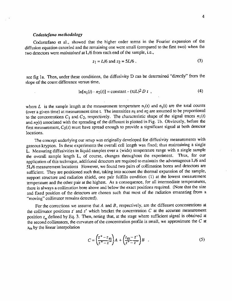
For the corrections we assume that A and B, respectively, are the diffusant concentrations at

the collimator positions z and z + which bracket the concentration C at the accurate measurement

position z,, defined by Eq. 3. Then, noting that, at the stage where sufficient signal is obtained at

the second collimators, the curvature of the concentration profile is small, we approximate the C at

Xm by the linear interpolation

(z+-Zm_ [z m- z-_

C = _z.-i..+-.S__z_ja+ _,z__z_jB(5)

_\ (a)

tracer 6 ' ' I]. zlocation zl z2

I

Radiation nl(t) ne(t)shield

• ! i ! •

pe (b)

8 .Time

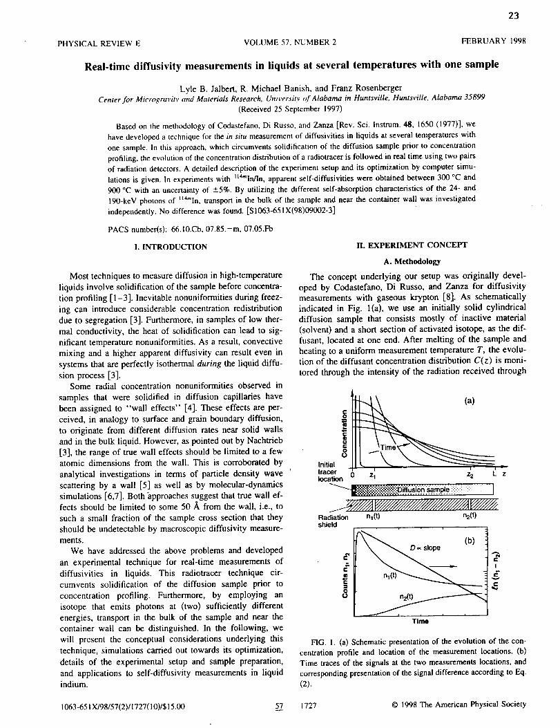
Fig. 1. (a) Schematic presentation of the evolution of the concentration profile and location of the

measurement locations. (b) Timetraces of the signals at the two measurements locations, and

corresponding presentaiion of the signal difference according to Eq. (2).

Extensive numerical computations showed that this methodology is very robust. The input

diffusivity could be recovered to with a few ) 0.1% even with + 2 standard deviations on the input

concentration (count rate) data.

Hardware Design and Construction (task 2)

Choice of radiation detectors

Since the experimental hardware developed for this project would be flown in a spacecraft the

initial requirements for the radiation detectors were:

• operational with cooling only to room temperature,

6

• asufficientlyhigh absorptioncoefficient,for thephotonsof interest,suchthatno morethan1cmof materialwouldbenecessary,

• spectralresolutionof betterthan5 keV,

• low energypedestalof nomorethan15-20keV

Theserequirements"limited" usto usingeithersolid statedetectors(i.e., CdTe, HgI2, Si) orinorganicscintillatorssuchas Tl-dopedNaI or CsI. Silicon was rejectedbecauseof its lowabsorptioncoefficientandlow spectralresolution. We thereforetestedthe following materials,high-pressurebridgman-CdTe,Cl-dopedCdTe,CdZnTe,high-pressurebridgrnanCdZnTe,HgI2,andTl-dopedCsI. In orderto testfor thefull rangeof photonenergies(bothhigh and low) thatwecouldusein our self-diffusionstudiesthesematerialsweretestedwith I_29(30, 40 and65 keVphotonenergy)Cd1°9(22 and 88keV), Am 2a_(60keV) andSe75(121, 136,264, 280, and400keV). Theselectioncriteriabetweenthevariousdetectorswerethepeakto valleyratios, thefull-width at half-max (FWHM) to the peak height, locationof the low-energy pedestal,and thespectralresolution.Thesematerialsweretestedatroomtemperatureup to 65°C.

Basedon the aboveselectioncriteria,CdZnTewas selectedas the detectormaterial. As asupplierwe choseeV Products,Inc. (Saxonburg,PA) which had done (andcontinues to do)extensivework in miniaturizingthedetectorcircuitry andnoisereduction.

Diffusion sample and ampoule

The considerations for the optimum length of the diffusion couple for a Codastefano based

methodology is different than for long capillary technique cells. In the Codastefano technique the

diffusivity is determined from the signal difference between the two (L/6 and 5L/6) detector

locations. Also, before valid measurements can begin, both the initial maximum "wave" of

diffusant must pass the first detector and a (statically) significant signal level must be present at the

second, far, detector. Thus, there is an optimal sample, and diffusant, length, such that

measurements are valid shortly after the maximum wave has passed the first detector and such that

the diffusant concentration is equalibrated (fully diffused) over a long enough time to allow for

multiple determinations. In addition, the sample diameter is optimized to allow for a reasonable

(radioisotope) activation parameter, i.e., if the isotopicaUy enriched portion is too small, a much

long activation time is required. Finally, the sample diameter should be large enough to allow us to

investigate the "wall effect". Following extensive numerical modelling we found that a 3 mm

sample with a 29 mm long native abundance section and a 1 mm radioactive tracer (diffusant)

portion sufficiently fulfilled the criteria.

Then, as indicated in Fig. la, we use an initially solid cylindrical diffusion sample which

consists mostly of inactive material (solvent) and a short section of activated isotope, as the

diffusant, located at one end. After melting of the sample and heating to a uniform measurement

temperature T, the evolution of the diffusant concentration distribution C(z) is monitored through

the intensity of the radiation received through two bores (collimators) in a radiation shield.

BN Ampoule design

The BN ampoule consists of four pieces and a graphite spring, see figure 2. The four pieces

are the ampoule body, bottom plug, plunger and screwcap, which are constructed from

Carborundum grade AX05. This high-purity grade BN is not wet by any of the metals under

consideration for this work. The ampoule body I.D. is reamed to 3.00, with tolerances of -0 and +

7

0.01mmto minimizeerrorsin the(total)samplelength. Theampoulebody O.D.variesdependingon thewall thicknessof theparticularoutercartridge. Thebottomplug is precisionmachinedto3.05+ 0.02 _ and 5.0 + 0.02 mm long. It is press fitted into the body, providing "square" corners

at the sample bottom. The plunger is individually fit to less than 0.02 mm clearance to the ampoule

body. Close tolerance between the plunger and the ampoule bore prevents liquid metal from

escaping. The low-force graphite spring pressing against the plunger

glass rod

insulation

screw lid

spring

plunger

silica cartridge

plug

10 mm

Fig. 2. Cross-section of diffusion sample cartridge.

ensures a flat interface at both ends of the sample. This ampoule is vacuum-baked at high

temperature to remove gaseous contaminants.

An outer cartridge provides a vacuum or gas seal to minimize oxidation or transport of the

diffusion couple. The specific material used varies depending on the temperature range and

radiotracer employed. Up to the present time, silica glass, aluminum and stainless steel have been

used for these cartridges.

Sample preparation

The native abundance section is prepared from 6N starting material. It is vacuum-cast (10 -6

mm Hg) in a 2.9 mm diameter BN mold to remove residual oxides, voids and gaseous

contaminates. It is then removed, trimmed and weighted to 0.1 mg. This section is then loaded

into the diffusion ampoule itself and vacuum cast again to approximately 100 °C above the planned

processing temperature. The final vacuum casting minimizes any voids and residual oxide in thematerial.

Theisotopica/lyenriched(diffusant)sectionis preparedinto a flat disk using a boron nitrideampouleconsistingof threepartsmachinedto tight tolerances.After loadingandassemblingtheampouletheisotopicallyenrichedmaterialis vacuummelted,againto approximately100 °Cabovetheplannedexperimenttemperature.It is thenremovedunder inert gas,weightedto 0.1 mg andsealedin asilicaglasstubefor neutronactivation.Theactivatedsectionis removedfrom the silicatube,underinert gas,andloadedinto theampoule.After replacingtheplungerandspring theBNampouleis mechanicallyclosedwith thescrewlid and insertedinto the (square-bottomed)outercartridge.

Isothermal liner I radiation shield

The Isothermal liner/radiation shield was to function as both a zone leveler, to minimize any

temperature nonuniformities across and along the diffusion sample, and as a collimator for the

emitted photons. As originally conceived LMD was to be flown as an "shuttle-independent" GAS

cannister experiment. Thus, both experiment mass and the power required for operation were to

be minimized. Gold was chosen as the liner/shield material due to its high thermal conductivity,

high radiation absorption and ready machinability. The initial liner/shield design yielded a cylinder

approximately 21 mm diameter (7 mm wall) and 90 mm long. Sixteen 0.67 mm collimators were

bored in a spiral pattern along the liner/shield axis. In order to minimize heat transfer, and

therefore, the input power required, considerable effort was devoted to reducing the convective and

radiative heat transfer. As presented at the LMD Science Concept Review (SCR) the liner/shield

was suspended by a wire "spokes". A series of gold-flashed thermal shields minimized the

radiative losses. With this design we were able to maintain sample temperatures of 800 °C with 20

watts. Assuming 28 V power (or batteries) this represented a current draw of less than 1 A.

However, in the first diffusion measurements with radiotracers excessive background through

the shield overwhelmed the signal (radiation) from the collimators. Thus, it was obvious that

either the shield wall thickness was not sufficient or that the collimation hole diameter was too

small; or both.

A series of experiments was run to determine the optimum collimator geometry. Both the

collimation bore diameter and the shield thickness were varied, between 1 and 3 mm, and 13 to 39

mm of Pb, respectively. A small collimation bore diameter gives high spatial resolution but a low

signal-to-background level; for a large collimation hole the converse is true. A thin shield

thickness (low bore length) has minimum scatter in the bore but high direct radiation penetration

and fluorescence. The results of these tests indicated that a 2 mm diameter collimation hole and a

16 mm bore length would provide the optimum s!gnal-to-background level for diffusion

measurements. Thus, the gold liner/shield that has been used for all measurements to date under

this contract has been 41 mm diameter, with an approximately 9 mm center bore (see below), 70

mm long. 2 mm diameter collimation holes are bored through the liner/shield at the required I_16

and 5L/6 positions.

Choice of Radioisotopes to be Used (task 3)

As stated above, an original objective of the LMD project was to development a measurement

methodology and flight hardware. Beyond suggesting individual elements or alloys for

investigation little justification was given for specific choices. The Science Concept Review panel

found this to be scientifically unsound. In response to this criticism, in preparation for submitting

to the next available NRA, we systematically searched the literature for possible liquid structure

9

featuresthatmayberesponsiblefor specificdiffusionmechanisms.Fromthis we selecteda seriesof elementsfor studybasedon their "class-like"self-diffusionbehavior.

Class-like self-diffusion behavior of molten elements

In spite of the large uncertainties in diffusivity data, enough insight has been obtained, in

particular through a few measurements spanning wide temperature ranges, to recognize some

class-like behavior that can be associated with temperature-dependent structure features of liquids.

D(T) data are conveniently tabulated in terms of the two parameters DO and Q in the relation

D = D Oexp(-Q/RT), where Q is understood only as an apparent "activation energy", without the

intent to support activated state theories. Such compilations of data, and corresponding plots of

In D vs. 1/T readily reveal a few cases of clear "non-Arrhenius" behavior, i.e. discontinuous, steep

increases of the diffusivity with temperature.

Tin, for instance, shows a sharp increase of D with rising T around 1030 °C [8]. This has

been associated with the dissociation of a second structure in the liquid [8]; see below. This

dissociation is indicated by the disappearance of a subsidiary peak in plots of the scattered X-ray

intensity versus scattering vector [9] and the appearance of a peak in the differential thermal

analysis curve [10]. Similarly, in liquid gallium, below 70 °C the Arrhenius plot yields a diffusion

"activation energy" of 1.1 kcal/mol, while at higher temperatures it is about twice this value [11].

Correspondingly, a subsidiary X-ray peak disappears at around 100 °C [12]. Mercury shows a

similar befiavior, with the disappearance of the second liquid structure and the sudden increase in

D(T) occurring at around 0°C [10]. Liquid tellurium, the only elemental liquid semiconductor (see

also [t3]), on the other hand, possesses a sharp decrease in the slope of D(T) with increasing

temperature around 500 °C, i.e. 50 °C above the melting point [14]. Again, neutron scattering data

suggest a structural transition around this temperature [15]. The initial steep slope in D(T) has

been interpreted in terms of the dissociation of chain-like structures and, thus, increased thermal

mobility of molecules in liquid tellurium, that is essentially completed around 500 °C [14]. In

contrast to these complex systems, the alkali metals as well as copper and silver show rather

monotonic D(T) behavior [3].

The above cases suggest that for liquid elements for which detailed diffraction and, thus,

structure data exist, valuable predictions of the D(T) can be made. Such structure data exist for a

large number of liquid metals and semimetals [16-18]. Most simple liquids and liquid metals

exhibit a sharp main peak in plots of scattered intensity versus scattering vector. Liquid metals

exhibiting a symmetrical sharp maximum (Saweda type-a) include the alkali metals, Mg through

Ba, copper, silver, gold and the transition metals. Symmetrical main peaks, which are also

obtained from hard-sphere-interaction diffraction models [18], indicate complete randomness in

atom arrangement, i.e. no preferred configuration of atoms, however transient [ 16].

In several liquid metals, the first scattering peak is asymmetrical (Saweda type-b [18]), and in "

some cases has a pronounced shoulder on the high-angle (lower atomic distance) side of the peak

(Saweda type-c). This group includes, in addition to Sn, Ga and Hg mentioned above, Zn, Cd,

Si, Ge, Sb, and Bi, with possible minor asymmetries in the peaks of In [19] and Tl [20]. Note

that both Ge and Si, which are semiconductors in the solid state, tum metallic on melting [ 13]. In

the non-metallic liquids Se and Te, which show predominantly covalent (homopolar) bonding, this

subsidiary peak is particularly pronounced. Thus the probability of finding an asymmetric

maximum is higher in elements of the higher groups, in which the solid-state bonding is

predominantly non-metallic [21]. The distance values corresponding to, these subsidiary peaks

10

oftenrepresentsthenearest-neighbordistancecharacteristicof thecovalentbondin thesolid state,e.g. gray tin in the Sn-system,while the mainpeak closelycorrespondto the distancein themetallically-bondedsolid, e.g. white tin. This suggeststhatin theseliquids thereis a short-termlocalizationof valenceelectronsin boundstatesbetweenpairs or groups of neighboringatomswithin anotherwisecompletelyrandommetallicallybondedmatrix. With increasingtemperature,the formationof short-livedclustersbecomesless likely, leading to the disappearanceof thesubsidiarydiffractionpeaks.Evenmorepronouncedthanin Se and Te, liquid sulfur (an insulator)

shows on heating several structural transitions, between various molecular ring and chain

configurations, over a range of more than 100 °C above the melting point [22,10]

High�Low energy photons for "wall effect" investigations

In addition to its real-time feature, this isotopic labeling technique permits investigations of the

perceived "wall effect" mentioned above. By employing an isotope which emits photons at two

sufficiently different energies and, thus, different self-absorption behavior, transport in the bulk of

the sample and near the container wall can be distinguished to some extent. For example, based on

attenuation data, for the 24 keV and 190 keV photons of 114mIn [23] we have calculated the

fraction of the total radiation received at the two different emission energies outside a 3 mm thick

sample vs. the distance of the emitter from the surface of the sample; for details of the one-dimensional slab model used see Refs.[24]. Note that the 24 keV photons received are predicted to

originate in essence only from a 300 I.tm deep surface layer. The 190 keV photons, on the other

hand, stem from throughout the whole sample slab. This behavior was experimentally confirmed_

for details see Jalbert, Banish, and Rosenberger at the end of this report. Thus, in selecting

elements for self-diffusion studies consideration was given to isotopes that emitted (multiple)

photons both high enough in energy to be representative of "bulk" diffusion and low enough to

represent trafisport in the "wall" region of the sample.

Systems to be used in diffusivity measurements

Based on the above considerations we proposed investigating the following systems.

• Simple liquids:

Indium which may show some weak nonmonotonic behavior, has a combination of low and

high energy photons that can be utilized for quantifying wall effects, a conveniently low

melting point and a wide liquid temperature range.

Rubidium has been studied over approximately 80% of its liquid state. However, the

temperature dependence of Rb has been reported as both T 2 and Arrhenius.

Aluminum based on neutron diffraction data aluminum is expected to have a monotonic

temperature dependence. However, aluminum self-diffusivity values are not available.

• Complex liquids:

Cadmium has two advantageous photons for studying bulk and wall transport.

Gallium with low melting point and wide liquid range with x-ray diffraction data showing a

pronounced asymmetry in the first peak.

Tin which has been extensively investigated on Earth and to some extent in space [2,8,9],

producing controversial results. It also has two particularly advantageous photons for

studying bulk and wall transport.

11

Tellurium and selenium, which should provide interesting features in D(T), due to the

multiple structures that are known to exist in their liquid states. Te has the advantage of

two distinctly different energy photons and Se that of a lower melting point. Note that

the energies of Te also appear well suited for wall effect investigations.

Convective Effects on Diffusivity Measurements (task 4)

Numerical modelling of magnetic fields to suppress convection

The scaling considerations presented above show that convection velocities in typical self-

diffusion experiments must be reduced to much less than 10 -5 cm -1. In principle, this can be

achieved in liquid metals using a steady magnetic field to damp the flow. In order to assess the

magnitude of the field required, we have computed buoyancy-driven flows in a model diffusion

cell geometry with and without applied magnetic field.

The 2D Navier-Stokes-Boussinesq equations were solved for flow driven by small lateral

temperature gradients in a vertical cavity of 5 cm length with a width of 1 and 3 mm, respectively.

As illustrated in Fig. 1, two types of lateral temperature boundary conditions were considere'dl In

case 1, a uniform temperature difference of either 0.1 or'0.01 K was applied'across the Slot. In

case 2, a "cold spot" of about 0.1 K was assumed at the upper right corner. Transverse and vertical

magnetic fields were considered and it was assumed that generation of secondary magnetic fieldsby the flow could be neglected. The two-dimensionality of the problem allowed us t-o neglect the

electric field [25].

The steady Navier-Stokes Boussinesq equations governing the transport of heat, mass and

momentum are written in dimensionless form as

8um+ u. Va = - Vp + PrV2u - RaPr0k - Ha2 (u×B)×B,Ot

and

V.u =0

(6)

(7)

(8)m+ u. VO = V20,8t

• . iii

where u(x,t) , B and 0(x,t) are the dimensionless velocity, magnetic field and temperature,

respectively, and Ra = _gATd3/K'v, Pr = v/_c and Ha = Bd(c/_) 1/2. The physical properties 13,

AT, d, _, _, p and v are, respectively, the thermal expansion coefficient, the maximum deviation

from the desired uniform temperature, the width of the slot, the thermal diffusivity, the electric

conductivity, and the dynamic and the kinematic viscosity. Ra, Pr and Ha are the Rayleigh,

Prandtl and Hartmann numbers, respectively.

The governing equations were recast in stream function vorficity form and discretized using a

Chebyshev pseudospectral collocation method with an Adams-Bashforth/second backward Euler

temporal scheme [26,27]. The discretized problem was solved using an influence matrix method

[26-28]. It is well known that at high values of the Ha the flow is confined to narrow boundary

layers with thickness proportional to Ha -lt2 for walls perpendicular to the field lines and Ha -1 for

walls parallel to the field lines [25]. Thus, we needed to ensure sufficient spatial resolution to

12

Case 1 Case 2

g{ 0 (x,1) = 1 -x 0 (x,1) = 1 -x

(o,z) = 1.

L

d

e (o,z)= 1

e (1,z)= o

0 (1 ,z) = 0 a (z)a=2cm O<Oa< 1.01

L-a

O(1,z)= 1,0<z< d

z

0 x 1

Figure. 3. Sketch of problem domain for both case 1 (lateral temperature gradient extends

throughout the domain) and case 2 (lateral temperature gradient on the right'hand wall only

extends over 2 cm).

capture the boundary layers. Collocated Chebyshev polynomials _ were distributed such that for

N+I points in a given 'coordinate direction xi = cos(in/N), i = 0,1 .... N.. We used 33x85

collocation points. This gave us 6 points inside 1.225 mm for the horizontal boundary layers (for

the 3 mm cell width) and 6 points inside 0.477 mm for the vertical boundary layers. Given that the

points are more closely spaced as one approaches the boundary, this appears to provide sufficientresolution for these flows.

Using the physical properties of liquid tin, we obtained solutions for both temperature

boundary conditions. The lateral magnetic fields were found to be the most effective for damping

the flow. This is because the main damping effect is on the velocity component perpendicular to

the field lines. In the absence of a magnetic field, the maximum velocity is the vertical component,

w. A vertical field is not as effective in reducing the w-velocity since it only directly damps the u-

component. Nevertheless, in the bulk of the domain, flow velocities are diminished and the flow

is squeezed close to the boundaries. Three sets of results for lateral fields are presented in Table 1.

For case 1, both cell widths were considered. Since for case 2, the 3 mm width velocities at high

Hartmann numbers were similar in magnitude to those in case 1 we did not carry out calculations

for 1 mm widths for this case. The flow velocities obtained in the absence of a magnetic field are

1The Chebyshev polynomials are defined as Tn(x) = cos(n arccos x), n : 0,1 ..... and -1 < x < 1.

13

aboutthesameasthosepredictedby theapproximationof Batchelor[29], i.e. - 10-2Ravdd.ForHa= 0 thecalculatedresultsscalelinearlywith adecreasein temperatureor with gravitylevel.

Summary

We have calculatedthe convectiveflow in diffusion cells arising from small horizontaltemperamregradientswith andwithout steady,transversemagneticfields. Only for high fields,on theorderof 1Tesla,couldvelocitiesbebroughtdown to the orderof 10-5cm s-1or less. Athighlateralfields themaximumvelocityis thehorizontalcomponent,which is typically twice theverticalmaximum.Sincetypicaldiffusivespeedswill beon theorderof 10-5crn s-1 (basedon v-D/L, where D is the diffusivity and L= 5 cm), it appearsthat, even for lateral temperaturenonuniformitiesaslow as0.01K, unlessacombinationof thin capillaries(lessthan 1 mm width)andlargemagneticfields (in excessof 1 Tesla)areused, the maximumflow speedscannotbereducedsignificantlybelowdiffusive speeds.

Table1:Convectionspeedsin diffusioncell modelwith andwithouttransversemagneticfield.

iiiiilil _ _!i iliiliiiiiii!iiiiiiiiiiii_!_i_iiiiiiiiii_iiiiii_i_i_iiiiiiiiiiii_ii_!ii_i_i_iiiiiii_i_iiiiiiiiiiiiiiiiiiii!AT = 0.1K Ha u w u w

0 0 1.13×10 -2 1.87×10 -2 0 1.23×10 -3 2.08×10 -3

10 0.1 3.26×10 -3 6.57×10 -3 0.29 3.62×10 -4 3.84×10 -4

50 0.5 6.5×10 -4 1.3×10 -4 1.47 3.32×10 -5 2.32×10 -5

100 1 1.29x 10 -4 5.01×10 -5 2.95 1.25×10 -5 6.09×10 -6

147 1.47 7.60×10 5 2.63×10 -5

AT = 0.01K

0 0 1.13×10 -3 1.87x10 -3 0 1.23×10 -3 2.08×10 -3

10 0.1 0.29 3.52×10 -5 3.838×10 -5

50 0.5 3.63×10 -5 2.07×10 -5 1.47 3.33×10 -6 2.31×10 -6

100 1 2.95 1.24×10 -6 6.098×10 -7

147 1.47 7.61×10 -6 2.63×10 -6

_i!_iiiii_i!iiii_iiiiiiiiiiiiiiiiiiiiiiiiiiiiiiiii_i_iiii_iii_iiiiiii_ii_iiiii_iiii!_iiiiiiiiiiiiiii:iiiiiiiiii:iiiiiiiiiiiiiiiiiiiiiiiiii:iiiiiiiii:iiiiiiiiiiiiiii:!iiiiiiiii:i:iiiiiiiiiiii:iiiiiiiiiiiiiiiiiiiiiiiiiiiiiiiiii:iiiiil:iiiiiiiiii:iiiiiiii:_i_iiiiiiiiiiiiiii_!i_ii_i_i_iiiiiiiiiiiiiiiiiiiiiiiii_iiiiiiiiiiiiiiiiiiiiiiiiiiiiii_ii_ii_ii!_!iiiiiii_i_iiiiiiiiii_ii_ii_i_i_ii!_i!i_i_!i_ii_iii_M!ii!ii!ii!ii!iii!_!iiiiiiiiiiiiiiiiiiiiiiiiiiii!iiiiiiiiii!ii!iiiiii!i_ ii

0 0 7.83×10 .3 9.73x10 3

10 0.1 2.61×10 -3 2.3910 -4

50 0.5 3.25×10 "4 1.77×10 -4

100 1 1.21×10 "4 4.88×10 -5

14

Numerical modelling of buoyancy-driven convection in diffusion cells

To provide more quantitative guidance for experimental work, we numerically modeled

diffusive-convective transport in vertical cylinders. The dimensions of the cylinders were chosen

to correspond to typical diffusion experiment geometries. Thermal boundary conditions with

slight asymmetries were imposed to simulate small deviations from isothermality. Since the

objective is to simulate convective effects on self-diffusion, the diffusant and sample were assumed

to have the same mass density. The three-dimensional time-dependent transport of the diffusant

(initially located at one end of the sample) was simulated for the physical properties of liquid

indium.

The liquid phase was assumed to be a Boussinesq fluid contained in a closed vertical circular

cylinder of length L and diameter 2R. Gravity acts along the cylinder axis. The temperature at the

vertical wall of the cylinder has the form: T(r,0,z) = (T l -T2)/2 -(T_ + Tz)(cos0)/2 + ATzz/L. Here

T 1- T 2 is the maximum lateral temperature difference across the cylinder at any height z, and AT z is

the temperature difference between the bottom and the top. The temperature of the latter are T(r, 0,

0) = (T_ -T2)/2 - (T1 + T2) r (cos0)/2R and T(r, 0, L) = T(r, 0, 0) + ATz, respectively, The

governing equations for the time-dependent transport of heat and momentum in the system were

solved using finite difference on an equally spaced mesh and on a variably spaced mesh using the

code CFD2000 which is based on the finite volume method.

Summary

The simulation yielded various results of practical consequence. We found that, even for

temperature nonuniformities T_ -T 2 as low as 0.1 °C, convective transport in capillaries of 1 mm

diameter can largely exceed diffusion. Furthermore, the convective contribution to transport may

be increased by "stabilizing" ATz's. Hence, the widely used approach of keeping the top of

diffusion samples slightly warmer than the bottom appears to be a dubious means of "preventing

convection". Most striking, we found that diffusive-convective transport can result in profiles of

the radially averaged concentration values that are analytically indistinguishable from pure diffusion

profiles. This finding casts considerable doubt on various geometrical criteria previously used to

demonstrate the absence of significant convective contamination diffusivity data plots. In

summary, reduced gravity conditions are essential for definitive diffusivity measurements in liquid

phases of macroscopic dimensions. For details of this work see (Alexander, Ramus and

Rosenberger).

15

Risk Mitigation Flight Opportunity

A simpler version Liquid Metal Diffusion experiment was selected for a flight opportunity

under the NASA/Mir Glovebox/MIM risk mitigation program. The scientific and technological

goals of this phase were:

• Determination of the effects of steady residual gravity and g-jitter aboard spacecraft on

liquid diffusivity measurements.

• Determination of the influence of g-level on possible "wall effects".

• Test of anchoring technology to prevent void/bubble formation in liquid metal diffusion

samples at low gravity.

• Tests of a sample exchange technique for multiple runs of a diffusivity measurement setup

during a spaceflight.

• Test of radiation detector performance with respect to space background radiation level and

sample activity requirements.

The LMD hardware utilized the (Canadian Space Agency) Microgravity Isolation Mount

(MIM) as part of the Mir Space Station. The MIM hardware provided a unique opportunity for

testing the effects of residual gravity and g-jitter on liquid diffusion sample. It provided for

vibration isolation and defined g-inputs up to 10 .3 go; as well its' latched configuration; where g-

gitter and residual accelerations would be transmitted to the samples.

To take full advantage of the MIM capabilities, five H4"In/In metal self-diffusion samples were

flown. All samples were to be processed at 185 °C. (Note, initially the samples were to be

processed at 200 °C. However, because of concerns from the Russian Space Agency, the

processing temperature was decreased to 185 °C) The operating characteristics of the MIM during

sample processing were to be:

• One sample with the MIM latched down, .

• two samples with isolation only,

• one sample with 10 .3 to ].0 "2 go pulses, at approximately 0.01 Hz, normal to the sample axis,

• one sample with 10 .3 to 10 .2 go pulses, 0.01 Hz, perpendicular to the sample axis.

The design and construction of the flight hardware employed the same systems and

technology used for ground-based experiments. Containment and electronic redundancy

requirements that were placed on the hardware did not change its functionality. Additional samples

were contained in a hand operated storage carousel not typically used on the ground. Figure 4 is a

scaled cross-section of the flight hardware indicating the major components.

16

/8

Figure. 4. Liquid metal diffusion apparatus cross-section: (1) diffusion sample in cartridge, (2)heated isothermal liner/radiation shield, (3) CdZnTe detector pairs, (4) preamplifiers/energydiscriminators, (5) circuit board, (6) carousel with four additional sample cartridges, (7) lead pig,

(8) sealed aluminum housing.

Application of technique to indium: ground-based and low-gravity results

Indium was chosen as the first element for investigation due to its:

• low melting point of 156 °C,

• high boiling point of approximately 2000 °C, thus, giving a very wide liquid range,

• radioisotope having low (24 keV) and high (190 keV) photons with a high enough

branching ratio such that activation was relatively straight forward. The energy range of these

photons was such that wall effects could be investigated.

Diffusivity determinations were performed at a single temperature as a verification of the

method and hardware, both on Earth and aboard the space station Mir. In the ground-based tests

17

wealsoinvestigatedtheeffectof theinitial sourceactivity levelson the signal-to-noiseratio. Allexperimentswere run until diffusant/emitteruniformity was obtainedthroughout the sample.Typically thisrequires100hoursatthelow temperaturesusedin theseexperiments.

Thefirst five ground-basedrunswereperformedat temperaturesnear200 °C. In theseearlyexperimentsthetemperaturecontrolwith a manuallyadjustedDC power supply wasnot optimal.Indium sampleswith roomtemperaturelengthsof 30 mm anddifferent initial sourcethicknessesand activitieswere used. Radiationcounts were takencontinuously and summedevery 10seconds.Diffusantsourceparametersandapparentdiffusivity resultsaresummarizedin Table2.

Table2. Summaryof ground-basedresultsat 200°C.

Sourceactivity

[l_Cil

53

75

150

600

5000

Self-diffusivitiesin indium[10-5 cm2/s]

Left detectors

190keV 24keV

2.44+0.16 (3.74)*

2.60+0.17 2.47+_0.16

2.46+_0.16 (3.69)*

2.14+0.14 2.16+0.14

2.33+_0.15 2.04+_0.13

Rightdetectors

190keV 24keV

(only onepair used)

2.64+_0.17 2.43+_0.16

2.46+_0.16 (2.36)*

2.21+0.14 2.24+0.14

2.24_+0.14 2.06+0.13

* groundloop/straycapacitanceproblems:calibrationshiftsduringexperiment.

After athoroughexaminationof therawdataandcalculateddiffusivitiesan initial activity of 1mCi waschosenassufficientfor singletemperaturemeasurements.Using this activity, sampleswerepreparedfor the liquid elementdiffusion(LMD) experimentson spacestationMir

Four of the five diffusion samplesdeliveredto Mir wererun. Datafrom three testswerereturned. Datafrom thesecondsamplewas lost dueto softwareproblems;thefifth samplewasnot run due to Mir time constraints,i.e., defined input g-pulse runs were not carried out.Therefore,insteadof theMIM operatingconditionsstatedabovetwo sampleswererun in latchedmode,i.e.,without g-jitter isolation,samples1and3. Run2 wasperformedwith active isolation.Table1showsour low temperature(approx.200°C) indium self-diffusivity valuesboth at normalandlow-gravity (lessthan10"4- 10.6go)-

18

Table3. LMD Mir results.

Run

l(latched)

2(isolated)

3(latched)

Temperature

[oC]

186.5 + 0.8

185.0 + 0.4

186.5 + 0.4

Self-diffusivities in indium [ 10 -5 cm2/s]I

Left detectors [ Right detectorsI

190 keV 24 keV [ 190 keV 24 keV

1.99_+0.13 2.07+0.13 1.98+0.13 2.06+0.13

2.09+0.13 1.98_+0.13 2.07_+0.13 *

2.08_+0.13 2.09+0.13 2.05+0.13 *

* ground loop/stray capacitance problems: calibration shifts during experiment.

Discussion of low temperature results

The average (normal gravity) values of the self-diffusivity of In_14"/In at 185 °C are;

• 2.22 + 0.159 (for 190 keV photons) and,

.° 2.11 + 0.154 x 10 s c.m2/sec, (for 24 keV photons),

(The normal gravity values in Table 21 were corrected to 185 °C by the factor 1 x 10 "7cm2/sec]K.)

The average, low-gravity, indium self-diffusivity values are;

• 2.04 + 0.047 (for 190 keV photons) and,

o 2.04 + 0.044 x 10 .5 cm2/sec (24 keV"photons).

These low temperature experiments established that this technique and hardware will provide

accurate diffusivity data in element liquids. Several aspects are noteworthy. First, within the

experimental uncertainty, the results are reproducible. Furthermore, the agreement between the left

and right detector pairs, see Tables 2 and 3, indicates that at these low temperatures either

convective transport contributions are insignificant or, less likely, affect the concentration

distribution in the measurement plane rather symmetrically. The latter could result from a

convection roll that is oriented normal to the plane of measurement. The reduced spread of the

low-gravity data, while the D,'s themselves are not that different, are difficult to unambiguously

explain. Similar results have been noted by other authors [30]. While, there may be some

convective contributions (in the ground based data) to the apparent diffusivity, they are probably

nonsteady and, therefore, difficult to characterize fully, or eliminate.

Given the low scatter and reproducibility of the reduced-gravity data we report these values

with good confidence. Therefore, we do not see a need to measure these values again. The

reproducibility between the isolating and latched runs indicates, coupled with our numerical

modelling, that the LMD cell W_ isothermal to better than 0.1°C, which was a design goal.

Overall, these results are on the low end of the range of published values for DIn(200°C)

which are from (2.2 - 3.8 ) x 10 -5 cm2/s. Finally, it should be noted that for all data, transport in

the bulk of the sample and near the container wall were indistinguishable, i.e., no 'wall effect' was

detected.

19

Risk Mitigation Results

The overall results from this flight opportunity were very positive and for most aspects the

experiment was a success. In addition to the low temperature indium self-diffusivity results:

1) the sample exchange and positioning mechanism worked properly,

2) the radiation detectors worked well within specifications,

3) the chosen sample activity was acceptable for the (Mir) background radiation environment,

and

4) the sample containment/restraint system work properly.

Summary

During the course of this work, most of the proposed objectives were successfully completed.

We did not pass our Science Concept Review and, therefore, we did not build and fly hardware

capable of measuring diffusivities of several elements over a wide temperature range. However,

we did develop a methodology for this that has been demonstrated on the ground over a wide

temperature range. This same Codastefano methodology was successfully used for our low

temperature spaceflight results. Hardware components, radiation detectors, isothermal liner/shield,

etc., were also developed during this project. Numerical modelling showing the extreme

sensitivity of diffusion measurements to convective contaminations was completed. Finally,

numerical modelling of the self-defeating nature of magnetic fields to suppress convective

contaminations, in diffusivity measurements, was also completed.

20

References

[1] P. J. Dunlop, B.

[2]

[3]

[4]

[5]

[6]

[7]

[8]

[9]

[10]

[11]

[12]

[13]

[14]

[15]

[16]

[17]

[18]

[19]

[20]

[211

[22]

[23]

[24]

[25]

[26]

J. Steel and J.E. Lane, in Physical Methods of Chemistry, ed. by A.

Weissberger and B. W. Rossiter (Wiley, New York 1972) Vol. I, Part IV, p. 205-349.

G. Frohberg, in Materials Sciences in Space, ed. by B. Feuerbacher, H. Hamacher and R. J.

Naumann (Springer, Berlin 1986) [a] p.93-128 and [b] 425-446.

M. Shimoji and T. Itami, Atomic Transport in Liquid Metals (Trans Tech Publications,

Aedermansdorf, Switzerland 1986).

G. Careri, A. Paoletti and M. Vincentini, Nuovo Cimento X, 4050 (19580.

N.H. Nachtrieb, Berichte Bunsenges. 80, 678 (1976).

N.H. Nachtrieb, Self-diffusion in liquid metals, in Proceed. Internat. Conf. on Properties inLiquid Metals (Taylor and Francis, London, 1967) edited by Adams, Davies and Epstein, p.309.

P. Codastefano, A. Di Russo and V. Zanza, Rev. Sci. Instrum. 48, 1650 (1977).

J.P. Foster and R.J. Reynik, Met. Transact. 4, 207 (1973).

K. Furukawa, B.R. Orton, J. Hamor and G.I. Williams, Phil. Mag. 8, 141 (1963).

J.P. Foster, C. Daniels and R.J Reynik, Met. Trans. 6A, 1294 (1975).

S. Larsson and A. Lodding, in Diffusion Processes, ed. by J.N. Sherwood et al. (Gordonand Breach, N.Y. 1971) vol. 1, p.87.

A.H. Norten, J. Chem Phys. 56, 1185 (1972).

J.E. Enderby, in Amorphous and Liquid Semiconductors, edited by J. Tauc (Plenum, NewYork, 1974) Chpt. 7.

D.H. Kurlat, C. Potard and P. Hicter, Phys. Chem. Liqu. 4, 183 (1974).

F. Friedel and G. Cabane, J. Physique 32, 73 (1971).

J.R. Wilson, Met. Rev. 10, 381 (1965).

W.H. Young, Can. J. Phys. 65,241 (1987).

Y. Waseda, The Structure of Non-crystalline Materials (McGraw-Hill, New York, 1980).

H. Ocken and C.N.J. Wagner, Phys. Rev. 149, 122 (1966).

N.C. Halder and C.N.J. Wagner, J. Chem Phys. 45, 482 (1966).

W. Hume-Rothery and G.V. Raynor, Structure of Metals and Alloys (XX, London 1962).

F.A. Cotton and G. Wilkinson, Advanced Inorganic Chemistry, Third Edition (Interscience,

New York, 1972) p. 425.

W.H. Tait, Radiation Detection (Butterworths, London 1980).

Tsoulfanidis,N., Measurement and Detection of Radiation, (McGraw-Hill, Washington,1983).

T. Alboussiere, J.P. Garandet and R. Moreau, Buoyancy-driven convection with auniform magnetic field. Part 1 Asymptotic analysis, J. Fluid Mechanics, 253 (1993) 545.

J.I.D. Alexander, S. Amiroudine, J. Ouazzani and F. Rosenberger, Analysis of the low

gravity tolerance of Bridgman-Stockbarger crystal growth II: Transient and periodicacceleration, J. Crystal Growth 113 (1990) 21.

21

[27] J.M.Vanel,R. PeyretandP.Bontoux,A pseudo-spectralsolutionof vorticity streamfunctionequationsusingtheinfluencematrix technique,in Numerical Methods for FluidDynamics H, K.W. Morton and M.J. Baines, eds. (Clarendon Press, Oxford, 1986) 463.

[28] J.P. Pulicani, A spectral multi-domain method for the solution of 1D Helmholtz andStokes type equations, Computers and Fluids 16 (1988) 207.

[29] G.K. Batchelor, Heat transfer by free convection across a closed cavity between verticalboundaries at different temperatures, Q. J. Appl. Math. 7 (1953) 209.

[30] Smith, R. W. and Zhu, X., Materials Science Forum, 215-216, 113 (1996).

22

Papers published and submitted for publication

L.B. Jalbert, R.M. Banish and F. Rosenberger, Real-time Diffusivity Measurements in

Liquids at Several Temperatures with one Sample, Phys. Rev. E 57 (1998) 1727.

L.B. Jalbert, F. Rosenberger and R.M. Banish, On the Sensitivity of Liquid Diffusivity

Measurements to Deviations from 1-D Diffusion, J. Phys.: Cond. Matter 1_.9_0(1988) 1.

R.M. Banish, L.B. Jalbert, and F. Rosenberger, Self-diffusivity Measurements in Liquid

Indium at 185°C on the Mir Space Station, in preparation for publication in Microgravity

Science and Technology.

J.I.D. Alexander, J-F. Ramus and F.Rosenberger, Numerical simulations of the convective

contamination of diffusivity measurements in liquids, Microgravity Sci. and Tech. 9 (1996)

158.

Invited Presentation

Self-diffusion in Liquid Elements, Institut fur Werkstoffe and Verarbeitung, Technische

Universitat Munchen, Garching, 2 February 1998.

Numerical Simulation of the Convective Contamination of Diffusivity Measurements in

Liquids, Royal Institute of Technology, Stockholm, Sweden, 10 June, 1997.

On the Convective Contamination of diffusivity Measurements in Liquids, Joint Xth European

and Vith Russian Symposium on Physical Sciences in Microgravity, St Petersburg, Russia,

15-21 June 1997.

Real-time Radiotracer Diffusion Measurement Technique, Royal Institute of Technology,

Stockholm, Sweden, 13 June, 1997.

Real-time Radiotracer Diffusion Measurement Technique, Spacebound 97, May 11-14,

Montreal, Canada.

On the Convective Contamination of diffusivity Measurements in Liquids, Spacebound 97,

May 11-14, Montreal, Canada.

Materials Science in Mircogravity, Festkolloquium fur Professor Langbein, ZARM, Bremen,

14 February, 1997.

Real-time Radiotracer Diffusion Measurement Technique, 35th Aerospace Sciences Meeting,

Reno, NV January 6-9, 1997

On the Convective Contamination of diffusivity Measurements in Liquids, 35th Aerospace

Sciences Meeting, Reno, NV January 6-9, 1997

Real-time Radiotracer Diffusion Measurement Technique, 31 th COSPAR Scientific Assembly,

Birmingham, England, July 18-24, 1996

Real-time Radiotracer Diffusion Measurement Technique, 31th SPIE Meeting, Denver, CO,

July 8-12, 1997

23

PHYSICAL REVIEW E VOLUME 57. NUMBER 2 FEBRUARY 1998

Real-time diffusivity measurements in liquids at several temperatures with one sample

Lyle B. Jalbert, R. Michael Banish, and Franz RosenbergerCenter for Microgravity and Materials Research, Universio, of Alabama in Huntsville, Huntsville. Alabama 35899

(Received 25 September 1997)

Based on the methodology of Codastefano, Di Russo, and Zanza [Rev. Sci. Instrum. 48, 1650 (1977)], we

have developed a technique for the in situ measurement of diffusivities in liquids at several temperatures withone sample, in this approach, which circumvents solidification of the diffusion sample prior to concentration

profiling, the evolution of the concentration distribution of a radiotracer is followed in real time using two pairsof radiation detectors. A detailed description of the experiment setup and its optimization by computer simu-

lations is given. In experiments with It4"in/In, apparent self-diffusivities were obtained between 3130°C and

900 °C with an uncertainty of +-5%. By utilizing the different self-absorption characteristics of the 24- and

190-keV photons of 1_4"ln, transport in the bulk of the sample and near the container wall was investigatedindependently. No difference was found. [S1063-65 IX(98)09002-3]

PACS number(s): 66.10.Cb, 07.85.-m, 07.05.Fb

i. INTRODUCTION

Most techniques to measure diffusion in high-temperature

liquids involve solidification of the sample before concentra-

tion profiling [1-3]. Inevitable nonuniformities during freez-

ing can introduce considerable concentration redistribution

due to segregation [3]. Furthermore, in samples of low ther-

mal conductivity, the heat of solidification can lead to sig-

nificant temperature nonuniformities. As a result, convective

mixing and a higher apparent diffusivity can result even in

systems that are perfectly isothermal during the liquid diffu-

sion process [3].Some radial concentration nonuniformities observed in

samples that were solidified in diffusion capillaries have

been assigned to "wall effects" [4]. These effects are per-

ceived, in analogy to surface and grain boundary diffusion,

to originate from different diffusion rates near solid walls

and in the bulk liquid. However, as pointed out by Nachtrieb[3], the range of true wall effects should be limited to a fewatomic dimensions from the wall. This is corroborated by

analytical investigations in terms of particle density wavescattering by a wall [5] as well as by molecular-dynamics

simulations [6,7]. Both-approaches suggest that true wall ef-fects should be limited to some 50 A from the wall, i.e., to

such a small fraction of the sample cross section that they

should be undetectable by macroscopic diffusivity measure-ments.

We have addressed the above problems and developed

an experimental technique for real-time measurements of

diffusivities in liquids. This radiotracer technique cir-

cumvents solidification of the diffusion sample prior to

concentration profiling. Furthermore, by employing an

isotope that emits photons at (two) sufficiently different

energies, transport in the bulk of the sample and near the

container wall can be distinguished. In the following, we

will present the conceptual considerations underlying this

technique, simulations carried out towards its optimization,

details of the experimental setup and sample preparation,

and applications to self-diffusivity measurements in liquidindium.

II. EXPERIMENT CONCEPT

A. Methodology

The concept underlying our setup was originally devel-oped by Codastefano, Di Russo, and Zanza for diffusivitymeasurements with gaseous krypton [8]. As schematically

indicated in Fig. l(a), we use an initially solid cylindricaldiffusion sample that consists mostly of inactive material

(solvent) and a short section of activated isotope, as the dif-fusant, located at one end. After melting of the sample and

heating to a uniform measurement temperature T, the evolu-tion of the diffusant concentration distribution C(z) is moni-

tored through the intensity of the radiation received through

t-OOc-O¢o

Initialtracerlocation

Radiationshield

(a)

_o

I 111

0 z1 z2 L z

nl(t) n2(t)

ope (b)g- i

TI_

FIG. 1. (a) Schematic presentation of the evolution of the con-centration profile and location of the measurement locations. (b)Time traces of the signals at the two measurements locations, and

corresponding presentation of the signal difference according to Eq.(2).

1063-651XI98157(2)11727(10)1515.00 5"/ 1727 © 1998 The American Physical Society

1728

I,I. 2

JALBERT, BANISH, AND ROSENBERGER

lo .................... y0.9 /_0.8 24 keY ._keV

0.7 , .Ca_ulated -..

0.31t / .... = ^m-1

0.2} / et190 = 2"5 em'l

O'IV ............. _....UO 0.5 1.0 1.5 2.0 2.5 3.0

Thickness of I_yer Considered [mm]

FIG. 2. Emission of 24- and 190-keV photons from 3-mm-thick

indium sample containing IL'_In versus distance of the emitting

atoms from the sample surface.

two bores (collimators) in a radiation shield. These intensi-

ties n t and n; are assumed to be proportional to the

concentrations Ct and C2, respectively. The characteristic

shape of the signal traces n t(t) and n2(t) associated with the

spreading of the diffusant is plotted in Fig. l(b).To satisfy the requirements of the algorithm used to

evaluate the diffusivity [8],' the radiation collimation bores

must be positioned at

zl=L/6, z2=5L/6, (1)

where'L is the sample length at the measurement tempera-ture. The diffusivity D is then calculated from the difference

of the signal traces using the relation

ln[n l(t) - n2(t)] = const- (1r/L)2Dt, (2)

where the constant depends on the concentration profile

Co(z) at the beginning of the measurement. Since the Co(z)does not explicitly enter the D evaluation, diffusivities can

be consecutively determined at several temperatures during

the spreading of the concentration profile in the same

sample. Obviously, before the first measurement, Co(z) musthave spread enough to provide a significant signal at bothdetector locations.

In addition to its real-time feature, an isotopic labeling

technique permits investigations of the perceived "wall ef-fect" mentioned in the Introduction. By employing an iso-

tope that emits photons at two sufficiently different energiesand thus different self-absorption behavior, transport in the

bulk of the sample and near the container wall can be distin-

guished to some extent. Figure 2 illustrates this approach.Based on the attenuation data for 24- and 190-keV photons

of lt4mln [9], we have calculated the fraction of the totalradiation received at the two different emission energies out-side a 3-mm-thick sample vs the distance of the emitter from

the surface of the sample; for details of the one-dimensionalslab model used see Refs. [10,11]. Note that the 24-keV

photons received are predicted to originate in essence onlyfrom a 300-/.tm-deep surface layer. The 190-keV photons, onthe other hand, stem from throughout the whole sample slab.

Thus, using an appropriate detector circuit with energy dis-

57

crimination capability (see Sec. IV C), transport near thewall of the sample container and in the sample bulk can be

distinguished to some extent.We have experimentally confirmed the above selective

absorption behavior. Indium disks of 100, 200, and 300/zmthickness were prepared from indium that had been uni-

formly diffusion doped with I t4mln. The normalized ratios ofthe 24- and 190-keV counts received from these disks agreed

well with the predicted values; see the data points on the

curves in Fig. 2.

B. Collimator positions and thermal expansion

Relation (2) is based on the specific location requirementfor the detectors given by Eq. (1) with respect to the sample

length L. For applications of this measurement technique atseveral temperatures with one sample, corrections are re-quired to account for thermally induced changes in sampledimension and collimator locations. For these corrections it

is advantageous to use two pairs of collimation bores anddetectors. They are positioned such that, taking into accountthe thermal expansion of the sample, support structure, andradiation shield, one pair fulfills condition (1) at the lowestmeasurement temperature and the other pair at the highest.As a consequence, for all intermediate temperatures, there is

always a collimation bore above and below the exact posi-tions required. (Note that the size and fixed position of .thedetectors is chosen such that most of the radiation emanatingfrom a "moving" collimator remains detected; see also Sec.

IV B).For the corrections we assume that A and B, respectively_,

are the diffusant concentrations at the collimator positions z

and z + that bracket the concentration C at the accurate mea-surement position z_ defined by Eq. (1). Then, noting that, atthe stage where sufficient signal is obtained at the secondcollimators, the curvature of the concentration profile is

small, we approximate the C at zm by the linear interpolation

C = I Z_z _ ) A + _ z_z _ ] . (3)

Ill. EXPERIMENT SIMULATION AND OPTIMIZATION

We have carded out detailed computer simulations to op-timize the experiment setup with respect to sample size and

activity, measurement accuracy, and number of D(_ dataobtainable with one sample. In the following we derive thebasic relations used; for more details on the simulations thereader is referred to Ref. [10].

A. Evolution of concentration distributions

including sample expansion

In a realistic simulation of the experiments, changes in

sample length due to thermal expansion during heating to thefirst measurement temperature and heating or cooling to con-

secutive temperatures must be taken into account. Let theinitial concentration profile in the sample of total length L1 at

temperature T1 be

g(z)=CoO(z-li), 0<z<Ll, (4)

with Co the initial concentration over the initial length of theactivated section I i and O(z-li) a step function equal to 1

for z<l i and 0 for z>li. With this initial condition and the

closed-system boundary condition

57 REAL-TIMEDIFFUSIVITYMEASUREMENTSIN ...

C:(O,t)=C:(Lt,t)=O, O<t, (5)

assuming that the diffusivity D is independent of concentra-tion and coordinate z, one obtains from Fick's second law

C,(z,t) = OCu(z,t) (6)

a general solution for the evolving concentration distributionin the form [12]

C(z't)=a°+n=tE a. cos -'-_-i ]exp[-_ L, ] ], (7)

z////_/./_ .///#/d//,_/_/

with the Fourier coefficients

1

ao=_l I f:'g(z)dz (8)

and

2 eL, [nlrz\

an-Ll(9)

Thus, after time t I at T1 with diffusivity D i,

Col, 2CoCt(z,t,): "-_-i + _=, n-"_"sjn_--_--i ]cos/---_'-i }

.X exp[_ / n'a'\ 2 ]o,,,] (,0)Next we assume that during the transition from T l to a

T2, the diffusive redistribution i.s insignificant. In view ofhe high ratio of thermal to solutal diffusivity of the mate-rials under consideration, this is readily achievable in

practice with rapid temperature ramping. Furthermore, weignore the diffusant redistribution due to the thermal ex-

pansion or contraction of the sample during the tempera-ture change. With typical thermal expansion coefficientsof liquids, this simplification introduces significant errors

only for simulation temperature changes in excess of 200 °C.Based on these assumptions, the initial condition at T2is taken as

g2(z)=Cl(z,tl). (11)

Thus, accounting for the new sample length L 2 , Eqs. (7)-(9)

yield for the evolution of the concentration distribution at T2

[10]

C2(z't)=a°2+,n:E am2 COS/--_''-2 }exp - D2t'

(12)

where

1729

.I. z=O

FIG. 3. Definition of sample-collimator-detector geometry forthe view factor calculation.

a02=o_ A,_ L I [nlrL2l,

Coli+ _ sin_ ----_--I] (13)LI .=1 L2 nrr

with

2C0 . [nlrlil [ [n_r] 2 ]

A =__ smt--_-] exp[-/Z-_-).._ O,,,] (14)

and

I n m

2C°li sin(m_-)+ _ "_2 " n mam2 = m _rL"_l n = I

L1 L2

sin + "R'L2

+ - . 05)n m

+Ll L2

Based on this formulation, we have simulated the evolutionof the concentration distribution during entire experiment

scenarios, including the multistep ramps to the first and con-secutive measurement tempeatures [10].

B. View factor, absorption of radiation, and detector noise

For realistic estimates of the radiation received at the

detector, the volume of sample visible through the col-limation hole must be known. Hence we have calculated

the view factor of the sample-collimator-detector geo-

metry [lO]. Assuming perfect absorption by the shieldmaterial, _radiation escapes only through the collimationbore of diameter 2re and length Lc; see Fig. 3. Under

this assumption, the number of emitters "seen" by the

detector is

i hcos-'( )-sin[2cos-( )llrC(z'2 ?rr_

dz dr dr, (16)

1730

where

Lc _" r,.)h= ( x/r2 c°s2 13+ :0-2(/s+ r sin 13)

q× 8(xfr 2 cos 2 fl+zo_r,.)" (17)

_2

_]/( r_c ) r2z0 = [Lc+2(!._+r sin 13)] - cos 2 13, (18)

r_=(L¢+ Is) and C(z) at the time of measurement is givenby an equation similar to Eq. (12). As defined in Fig. 3,

r,13,z are the coordinates within the sample, with z = 0 at theend containing the radiation source of initial thickness li.

The angle t=- _r/2 is taken in the direction of the detector

on the collimator axis.In the actual simulation runs, we have included the attenu-

ation of the radiation by both the emitter-location-dependent

self-absorption (see Fig. 2) and the thermal radiation shields

(see Fig. 6). Furthermore, the noise in the detectors, i.e., theuncertainty in the detector signals due to radiation countingstatistics, was accounted for. This noise is of the order of x/-n,

where n is the number of counts received. Thus the statistical

uncertainty increases with counts, but the relative uncertaintydecreases as l/x/-n [9]. Hence the higher the count rate, the

more accurate the results. This can be accomplished by either

using a long counting period or high initial activity.

C. Sample dimensions and activity

The lengths of the activated section li and the overall

sample L were optimized based on the following consider-ations. The above square-root dependence of the detector

noise on sample activity suggests the use 0f high activities to

maximize the resolution in the difference of the two detector

signals. This in turn minimizes the measurement time re-

quired at a given temperature and thus the errors from con-tinuous diffusion during a data acquisition period. Similarly,the initial activity required to ensure a given detector signalincreases with sample length. However, low activity levels

are desirable for radiation safety reasons. Simulation results

(see Sec. III E) showed that an initial activity of 5 mCi pro-vides sufficient resolution. With this initial activity, the op-

timum sample length is 30 mm [10].To determine the length of the activated section li we

recall our assumption that the part of the concentration pro-file viewed by a detector is linear; see Eq. (3). Thus the

initially activated section must be short engugh that the tran-sient in which the spreading concentration distribution pos-

sesses significant curvature is over when the signal level atthe second detector is high enough to begin measurements.The simulations yielded li= 1 mm as optimum. Thus our dif-

fusion samples consist initially of two parts: the I-turn-longradioactive section and a 29-mm-long non-activated section.

JALBERT, BANISH. AND ROSENBERGER 57

tion escaping through the collimation bores. Furthermore, ascan be seen from Fig. 3, due to the conical shape of the

radiation beam transmitted by the collimation bore, r,.'s

larger than the sample diameter will not result in a commen-surate increase of the radiation dose received by the detector.

These arguments are further complicated by the scattering ofand fluorescence induced by the primary radiation [9]. Our

samples (IL4"ln) emit about 95% yand 5%/3 radiation, with

the average/3 energy in excess of 750 keV. Both cause fluo-rescence in the shield. In addition, )' radiation is Compton

scattered in the shield and, in particular, upon grazing inci-

dence on the collimator surface. Each scattering process re-

duces the energy of the radiation. Thus multiple scattering

and fluorescence can lead to photons that are counted in en-

ergy windows different from those corresponding to the pri-

mary photons and fl particles.We have experimentally investigated various collimator

geometries for their effect on total radiation received by thedetector. Hence we used lead for the collimator optimization

experiments that were conducted at room temperature. Col-limation holes of 1, 1.5, 2, and 3 mm diameter were drilledinto lead shields of 12.7, 25.5, and 38.3 mm thickness. A

3-mm-diam cylindrical radioactive indium sample was

placed consecutively behind the collimation bores. The de-tector signals were energy discriminated; see Sec. IV C.Table I summarizes the results. The signal-to-noise ratio is

defined as the signal amplitude obtained in the energy win-

dow (+__0.3keV about the chosen energy) divided by the sum

of amplitudes measured in all other channels outside the en-

ergy window.From these data, we can draw the following conclusions.

Since the signal-to-noise ratio (SNR) for the l-mm collima-tor hole is essentially 1, the smallest usable diameter is 1.5

ram. As expected, with the 3-mm sample diameter very littleadditional radiation is received on expanding the collimatordiameter to more than 2 mm and, hence, the SNR remains

essentially unchanged or even decreases. Furthermore, the

signal-to-noise ratio increases with the increase in the thick-ness of the radiation shield, from 12.7 mm to 25.5 mm, while

a 38.3 mm thickness results in little further improvement.

Copper, initially planned as the high-temperature radia-tion shield material, showed intolerably high fluorescencelevels. For the actual high-temperature experiments, the ra-diation shield consisted of gold with a wall thickness of 15.5

ram. As calculated from absorption data [9], this wall thick-

ness provides the same absorption for 190-keV photons asthe 25.5 mm of lead used above. This results in an overall

diameter of the radiation shield/isothermal liner of 41 mm.With this collimator geometry and 10-mm square detectors,the maximum distance between the outside edge of the col-

limator and detector must not exceed 30 mm if all radiation

from the collimators is to be collected.

D. Determination of collimator geometry

Geometric factors as well as radiation properties of the

shielding material must be considered in optimizing the col-limator geometry. Obviously, the radiation shield must bethick enough to absorb a large fraction of the radiation. Oth-erwise the detector signal is not representative of the radia-

E. Simulated muititemperature experiments

Based on the above considerations, utilizing Eqs. (1)-(18)

evaluated for the optimized dimensions of our experimental

hardware, simulations were carried out to explore the feasi-

bility and accuracy of measurements at several temperatureswith the same sample. Table II shows for self-diffusion inindium that a temperature range of 700 °C can be covered in

57 REAL-TIMEDIFFUSIVITYMEASUREMENTSIN...

TABLE I. Signal-to-noise ratios obtained with various collimator geometries.

1731

Diameter Lead thickness Signal to noise ratio Signal to noise ratio(mm) (mm) at 24 keV at 190 keV

1 12.7 I.I 1.1

1.5 12.7 1.4 1.25

2 12.7 1.67 1.5

3 12.7 2.1 2.0

i 25.5 I 1

1.5 25.5 1.6 1.6

2 25.5 2.0 1.8

3 25.5 2.0 2.1

1 38.3 I I

1.5 38.3 1.9 1.5

2 38.3 2.2 1.9

3 38.3 1.7 2.2

100 °C increments using only two samples. The second col-umn lists the input diffusivities [13] used in the simulations.

The table illustrates well the importance of taking the detec-tor noise into account. Without superposition of noise on the

signals n l(t) and n2(t), the simulations unrealistically yieldan error in all eight deduced diffusivity values of less than0.2%; see the third and fourth columns. However, as shown

by columns six and seven, on superposition of a realistic

___(O)2,_ noise level, the errors increase to (a still very

acceptable) 1.5%.

Note that it is advantageous to begin with the highesttemperature and, thus, highest diffusivity in a measurement

series and then to take data at consecutively lower tempera-tures. Obviously, at the highest diffusivity the time required

until the signal at the second detector rises above backgroundis minimized; see Eqs. (7)-(9). In addition, the simulations

unexpectedly revealed another advantage of decreasing tem-perature sequences, in which the measurement time at eachtemperature is shorter than at the immediately following one.While at all temperatures the spreading of the concentration

profile depends on the product of the respective D and mea-

surement time [see Eqs. (7) and (12)], beginning with thesecond temperature there _s an additional time-dependent

spreading term [see Eq. (14)]. As a consequence, longermeasurement times at the prior temperature, as they would

be required in a sequence with increasing temperatures,

cause a larger decrease in the overall concentration gradient.The simulations show that the resulting smaller differences

between the two signals lead to fewer feasible temperaturesin an experiment.

The above simulations provided valuable guidance for ex-periment design. However, they do not account for some of

the error sources present in actual experiments. These in-clude imperfect shielding and secondary scatter by the radia-tion shield and collimation bores. In Sec. IV D we will

present procedures to at least partly correct for these errors

using signals from background detectors. There are also sig-nificant systematic errors associated with the dimensional

tolerances of the sample and collimator-detector geometry.These error sources are evaluated in Sec. IV E.

IV. EXPERIMENT

A. Sample preparation and containment

The sample consists of two parts: a short radioactive sec-tion and a long nonactivated section. The preparation and

containment of these sections is based on the following con-

siderations. Uncertainties in the sample geometry are the ma-jor error source in these experiments. Furthermore, the

sample cross section must be uniform to assure one-

TABLE II. Comparison of simulation model input diffusivities and simulation results for two model runsat eight different temperatures.

Input Result without noise Result with noiseTemperature

(°C) 105D (cm2/sec) 105D (cm2/sec) % error 105D (cm2/sec) % error range

900 10.2226 10.2002 0.22 10.2589 <0.5

700 8.260 01 8.255 02 0.060 8.185 63 < 1

500 5.978 81 5.978 31 0.0084 5.956 64 < I

300 3.456 23 3.456 21 0.000 72 3.498 95 < 1.5

800 9.280 63 9.25 65 0.26 9.331 37 <0.5

600 7.158 44 7.154 24 0.059 7.100 53 <1

400 4.734 12 4.733 54 0.012 4.723 77 < 1

200 2.210 22 2.2102 0.000 83 2.210 52 < 1.5

57JALBERT,BANISH,ANDROSENBERGER1732

Vacuum

V Weight

.fEndched_

isotopesample

ReadyloractivationBoronnitdde

crucible Readyto melt

FIG. 4. Steps for preparation of theenriched isotopepellet for

activation.

glass rod

:iberfrax insulation

screw lid

spring

_lunger

silica cartridge

section

dimensional diffusion. Nonuniformities in the cross section

can arise from capillarity (rounded edges at ends of both

sections) and voids or bubbles in the sample bulk and at theinterface between the two sample sections. Equally impor-tant is the accuracy in sample length and volume; see Sec.IV E. In addition, oxidation, in particular of the contacting

ends of the sections, can form a diffusion-resistant layer.

Hence, both the indium and boron nitride (BN) (Carborun-

dum grade AXO5) container parts (,BN is not wet by indium)are thoroughly high-vacuum baked (10 -6 mm of Hg at

900 °C) to remove gaseous contaminants.The radioactive section is prepared, as shown in Fig. 4,

using a boron nitride crucible consisting of three parts ma-chined with tight tolerances. After insertion of the bottom

plug into the 3-mm-i.d. cylinder, a bead of indium (40%enriched in It3In) is put in place. The weight of the bead is

chosen such that the thickness of the final disk will be ap-

proximately 1 ram. After insertion of the topplug, the wholecrucible, with a small weight on the top, is inserted into a

glass tube. This is followed by vacuum heating to 900 °Cand solidification of the sample under high vacuum while it

is compressed by the weight. After cooling, we backfill with

argon. Then the section is prepared for irradiation. Utilizinga glove box, the glass tube is broken and the sample is trans-ferred to a 3-mm-diam glass capillary. To facilitate sample

removal after irradiation, 5-mm-long rods are placed aboveand below the sample prior to sealing of the capillary. The

sealed-in section is then sent to the reactor for activation by

fast neutron irradiation.The 29-mm-long nonactivated section of the sample is

cast in place under high vacuum at 900 °C in the boron ni-

tride ampoule used for the diffusion measurements. As de-

picted in Fig. 5, this 7-mm-o.d. ampoule is 60 mm long andhas a 3-mm precision-reamed bore. To ensure the proper

sample length we require square corners on the top and bot-tom ends of the sample. At the bottom this is achieved by

press fitting a BN plug into the ampoule bore. At the top weapply a slight pressure on the sample with a weak graphitespring [Energy Science Laboratories, force 29.4 mN (3 g) at900 °C] against a BN plunger that has less than 0.025-mmclearance in the bore. To establish conditions that ensure theabsence of void formation, inactive sections were repeatedly

melted, solidified, and x-ray inspected.Then the activated section is transferred into the ampoule

in a glove box flushed with an inert gas. After replacing the

_ple

plug

10mm

FIG. 5. Cross section of diffusion sample cartridge.

plunger and spring, the BN ampoule is mechanically closedwith the BN screw lid and inserted into the square-bottom

silica tube, .which,.in turn, is evacuated and sealed.

B. Diffusion measurement apparatus

The apparatus, which accommodates the above sealed

diffusion sample cartridge, consists of the following com-

ponents (see also Fig. 6). There is a gold radiation shieldand isothermal liner (90 mm long, 41 mm in diameter).Gold was chosen because of its high melting point and

thermal conductivity together with the low fluorescence

and high radiation absorption properties. To minimize dis-

placement of this gold cell by thermal expansion it is sup-

ported by a silica pedestal (thermal expansion coefficient5.5x10 -7 cm/cm°C). There is a stainless-steel-encased,

ceramically insulated resistance heater (Fast Heat, 130 mm

long, 120 V, 5 A). To avoid radiation absorption, the heaterhas six holes (7 mm in diameter) at the positions of the

collimators and background detectors. Thermocouples (type

K) are inserted into the gold liner for temperature uniformitycontrol. One of these provides input to a temperature con-troller and silicon controlled rectifier that stabilizes the tem-

perature to better than +__0.5°C. An inner thermal radiationshield consists of a stainless-steel sheet. An outer thermal

shield consists of gold-coated boro-silicate glass. There aresix radiation detectors (not shown): one pair each aligned

with the oppositely placed, differently spaced radiation bores

(see Sec. II B) and one pair 90 ° off the measurement-detector

plane to record the background radiation. Top and baseplates contain the measurement structure. Axial heat lossesfrom the heated components to these plates are minimized by

Fiberfrax insulation.

57 REAL-TIMEDIFFUSIVITYMEASUREMENTSIN... 1733

'i.

ii

1.</;4.

Fiberfraxboard

Top plate/,

.',Ill A__J

Silicatube

/ Diffusionsample...-" carlridge

!Isothermalradiationshield(2 pairsofcollimationbores)

\ Gold-coatedsilicatube

"" Heatshield

"_Heater

"" Silicapedestal

Baseplate

FIG. 6. Cross section of diffusion measurement apparatus (with-

out detectors and electronics). Note the two pairs of collimationbores, offset with respect to each other, to cover the temperature

range 300 °C-900 °C for indium.

The temperature uniformity across the diffusion sample in

this apparatus was checked using a dummy diffusion samplecartridge with eight built-in, calibrated thermocouples (type

K, sheath diameter 0.5 mm, Omega Engrg.). At 500 °C, the

vertical temperature difference AT o across the indium

sample (see Fig. 5) was 0.4 °C, with the bottom cooler than

the top. At the same time the maximum horizontal ATh,

which occurred at about midla.eight of the sample, was0.3 °C. At 900 °C, we obtained a ATe= 1.4 °C of the same

orientation and a maximum ATh=0.4 °C at the top of the

sample.An important design c_onsideration for the use of the ap-

paratus over a wide temperature range is the thermal expan-

sion of the components, which changes the spacing of thecollimation bores and their position with respect to the de-

tectors. The changes in the bore spacing, which over a tem-

perature range of 700 °C is about 0.4 mm, is taken into ac-count when applying Eq. (3). The changing bore locations

with respect to the fixed detector positions are taken into

account by using detector crystals large enough that the ema-

nating radiation cone remains fully detected during the ther-

mal displacement.

(SCAs) per detector can be set using four potentiometers on

the circuit boards providing a 0-250 keV energy range.Due to differences in the characteristics of individual

crystals and detector circuits each detector must be indepen-

dently calibrated. The calibration is accomplished using a

multiple-channel analyzer (MCA) (Accuspec, NaI, CanberraInstruments) and a data acquisition system with a counter tot

each energy channel. The calibration of each detector SCA

energy window is performed by matching the SCA outputcount rate and the chosen MCA energy window count rate.

D. Measurement procedure

After loading the sealed sample ampoule into the gold cell

and repacking the thermal insulation, the temperature is

ramped at 15 °C/min to the highest experiment temperature.After the signal at the 5LI6 detectors has sufficiently risenabove background, data acquisition begins. The measure-ment times at this first and consecutive, lower temperatures

are predetermined based on the simulation results. After dif-

fusant uniformity has been obtained throughout the sample,we return to each experiment temperature and collect base-

line averages. These data are used to correct for inconsisten-cies of the detector crystals and possible abnormalities in the

collimator-detector geometry. One detector-channel is se-

lected as being "correct" and, using the averages at eachtemperature, all other channels are proportionally adjusted.The same is done with the two background detectors. The

background is subtracted from all channels and then Eq. (3)

is applied to find the concentration at all times.With sources activated to 5-10 mCi we can typically ob-

tain data at three separate temperatures per run. The simula-

tions suggested the feasibility of four temperatures. How-ever, in the simulation we did not allow for cool down

periods between temperatures. At lower temperatures theseperiods can be up to an hour for a 200 °C change.

E. Estimation of uncertainty in apparent diffusivity

As expressed in Eq. (2), the diffusivity D is obtained fromthe slope of a straight line fit to" ln[nl(t)-n2(t)]. We haveshown earlier that such straight line plots can be obtained

even in diffusion experiments with considerable convective

contamination [14]. Hence, considering the deviations from

isothermality of our samples (see Sec. IV B) and thus likely

resulting convective transport, the following estimate of un-

certainty in D must be understood with respect to the appar-ent rather than the true diffusivity. This uncertainty can be

expressed in terms of the uncertainties in the slope and the

sample length as [15]

(19)So= ,,Bj

C. Detectors, discriminators, and calibration

After examining numerous detector types, we have foundthat CdxZnl_xTe crystals (eV Products, 1 cm z and 3 mm

thick) provide a quantum efficiency of approximately 1 forthe 24-keV photons and 0.35 for the 190-keV photons ofindium. In addition, these detectors exhibit a low noise

threshold (_<10 keV) at temperatures _<50 °C, i.e., no addi-

tional cooling is required. Two single-channel analyzers

2 2where the slope B = - 7r2DIL 2 and trB = No'r/A, with N the

number of data points used in the fit, and A=N(Y._=it_)

(_,_i=lti) 2 and 2-[l/(N-2)]y_=l(yi-A-Bti) z, with- O'y-y = ln(n2-nl) and A (the y intercept)=const.

The uncertainty in the length of the sample can be esti-mated as follows. The sample is made of two sections (see

Sec. III C) producing an uncertainty

1734 JALBERT, BANISH, AND ROSENBERGER 5-/

TABLE III. Apparent self-diffusivities obtained with indium at

the Iwo photon energies in four experiments.

Temperature 190 keV 24 keV

(°C) ( 105D cm2/sec) ( 105D cm2/sec)

800 9.84 -+0.59 10.07---0.6 I

600 7.69-0.48 8.02-0.50

400 5.25-"0.34 5.01 ___0.34

700 7.72___0.47

500 6.20---0.39

300 4.60---0.33

900 8.95_+0.54 8.61 __+0.52

800 9.80-+0.59 10.16-+0.61

700 8.93 - 0.55 9.62 ---0.60

900 11.75--.0.70 11.63---0.59

600 8.04 _ 0.49 8.09 -+0.50

300 4.54 -+0.29 4.78 -+0.31

_L = _li + _INA, (20)

where /NA is the length of nonactivated sample. The uncer-

tainty in-the two sections is determined from the volume and

machining of the crucibles such that

_l = _V] + 6r , (21)

with r the radius of the crucible and V the volume of sample

material. If we assume that the density P is accurately

known, then the uncertainty in the volume is

(22)

The tolerance on the crucibles is "-_0.0127 mm (nominal

. sample inner diameter 3.01 ram). Due to the repeated

vacuum melting, the uncertainty in the masses is 0.001 g.

I t I I I I I I I

20_15

gg

[ 190o°CI _°C ,,. . I t h0.100 --200= 300 400

IIIlllllll

500 600 700 800 900 1000

Time [mini

FIG. 7. Original signal traces for 190-keV photons during the

9(_) °C-300 °C run.

8.8

8.6

8.4

._ 8.2

t 8.0

_ 7.8

7.6

7.4

7.2

7.02OO

• I l _ I I T I I i [ I I 1 I 1 I I !

I I I I I I I 1 I 1 I I I I I I 1 I J

220 240 260 280 300 320 340 360 380Time [min]

FIG. 8. Pitt of 600 °C data of 900 °C-300 °C according to Eq.

(2), together with diffusivities obtained from least-squares fits

(straight lines).

Substituting Eq. (22) into Eq. (21) and the result into Eq.

(20), the uncertainty in the length of the sample is - 1.02 mm

for indium.

The cr B error is directly related to the counting statistics.

This error is minimized with high initial activities. With the

activity levels chosen for these experiments we find that the

second term in Eq. (19) is up to an order of magnitude larger

than the first.

V. RESULTS AND DISCUSSION

Several diffusion runs with indium were carried out.

Each run covered three consecutively lower temperatures.

The results are summarized in Table III. The error esti-

mates are based on Eq. (19). The lack of 24-keV data for

the one run is due to failure of one low-energy channel. Note

that, within the uncertainty of the data, no difference be-

tween transport (diffusion) in the bulk and near the wall is

apparent.As-measured time traces of the 190-keV signals obtained

in the 900 °C-300 °C run (Table III) are shown in Fig. 7.

These plots reveal several features of the method. The right

top detector has the highest initial count rate since its posi-

tion z I = LI6 has been chosen for the highest T= 900 ° C, i.e.,

the longest L; see Sec. II B. The change in the diffusion

coefficient at the three temperatures is visible in the slope

changes of the data. Furthermore, the contraction of the

sample on temperature decrease is evident from the rise in

the count rate. One sees also that the final count rates of the

detectors differ, due to the individual characteristics of the

detector crystals; see Sec. IV D. A pitt of In(nl-n2) vs time,

resulting from similar curves obtained at 600 °C after their

base-line corrections, is shown in Fig. 8 together with the

least-squares fits for both energies.

All data from Table III together with the self-diffusivities

of In measured by other authors [4,13,16,17,18], are plotted

in Fig. 9. The wide scatter of the data illustrates well that

diffusivities obtained in liquids at normal gravity are prone

to be contaminated by uncontrollable convection. As empha-

sized for liquid diffusivity measurements by Verhoeven [19],

any horizontal component of a density gradient results in

convection without a threshold. We have recently estimated

5_7 REAL-TIME DIFFUSIVITY MEASUREMENTS IN... 1735

12

10

Eo 8'9,o

-t__. 4

2

0

v

V & •

,_I , I,,I,,,,I_ ,_, i,,,,i,,,]i,_ ,,i, _,,i,,,,i ,,,, I ,

V _ I _ AX

Y¥ •

_ X X

{t "

200 400 600 800 1000

Temperature [°C]

FIG. 9. Experimental data for self-diffusivities in indium: © this work; • Foster and Reynik [17]; A Lodding [13]; • Mathiak et al.[16]; V and • Carreri, Paoletti, and Vincentini [4] with !.6- and 0.83-mm-diam capillaries, respectively. Ogloblya, Lozovoi, and Chumakov[18] with 0.5-mm-diam capillaries.

convective contributions to transport in our experiments[14]. The numerical modeling results for self-diffusion inIn at 730 °C in 30-mm-iong capillaries, 3 mm in diameter,

show that at normal gravity convective contributions be-

come significant when an applied horizontal temperaturenon-uniformity ATh exceeds 0.01 K. Often, flow due to

horizontal density gradients can be reduced by keeping, as

is the case in our experiments (see Sec. IV B) the top ofthe sample slightly warmer than its bottom. However, theabove simulations [14] show that this can be rather ineffec-

tive and under certain conditions may even increase the ap-parent diffusivity.

From the above, it is not surprising that our data show

evidence of convection in the samples. For instance, the ap-parent D at 700 °C deduced from the 900 °C-700 °C run issignificantly higher than that of the 700 °C-300 °C run. This

may be due to the longer time the first sample was at hightemperature before the measurement at 700 °C was made.Thus there was more time for convective contamination of

the diffusive transport. Note, however, that the uncertainties

for the two measurements at 900 °C do not overlap. We as-sign this to possible inconsistencies in the sample prepara-

tion and convective contributions. The low value may be theresult of partial blockage of the diffusion path by either avoid or an oxidation layer between the active and inactive

sections of the sample.

IV. SUMMARY AND CONCLUSIONS

We have developed and systematically optimized a tech-

nique for the in situ measurement of diffusivities in liquids atseveral temperatures with one sample. This approach circum-

vents the solidification of the diffusion sample required byother methods, which can result in significant errors. In ex-

periments with 114=In]In, apparent self-diffusivities were ob-

tained between 300 °C and 900 °C with an uncertainty of+-5%. By utilizing the different self-absorption characteris-tics of the 24- and 190-keV photons of II_In, transport inthe bulk of the sample and near the container wall was in-

vestigated independently. No differences were found. Thereis clear evidence for convective contamination of our data.

To obtain increased accuracy in the diffusivity values, we

plan to perform these experiments in a low-gravity environ-ment.

ACKNOWLEDGMENTS

We thank W. F. Kaukler from our center for help with the

x-ray inspection of diffusion samples. L. Carver has expertlyprepared the figures. Support for this work by the Micrograv-ity Science and Applications Division of the National Aero-

nautics and Space Administration through Contract No.NAS8-39716 is gratefully acknowledged.

[I] M. Shimoji and T. Itami, Atomic Transport in Liquid Metals

(Trans Tech, Aedermansdorf, 1986).[2] N. H. Nachtrieb, Ber. Bunsenges. 80, 678 (1976).

[3] N. H. Nachtrieb, in Proceedings of the International Confer-

ence on Properties in Liquid Metals, edited by P. D. Adams,

H. A. Davies, and S. G. Epstein (Taylor and Francis, London,1967), p. 309.

[4] G. Careri, A. Paoletti, and M. Vincentini, Nuovo Cimento 10,1088 (1958).

[5] M. Fixman, J. Chem. Phys. 29, 540 (1958).

1736JALBERT, BANISH, AND ROSENBERGER

57

[6] S. B. Savage and R. Dai, Mech. Mater. 16, 225 (1993).

[7] G. Mo and F. Rosenberger, Phys. Rev. A 44, 4978 (1991).

[8] P. Codastefano, A. Di Russo, and V. Zanza, Rev. Sci. Instrum.

48, 1650 (1977).

[9] W. H. Tait, Radiation Detection (Butterworths, London 1980).

[10] L. Jalbert, Ph.D. dissertation, University of Alabama, Hunts-

ville, 1997 (unpublished).

[11] N. Tsoulfanidis, Measurement and Detection of Radiation

(McGraw-Hill, Washington, DC, 1983).

[12] J. Crank, The Mathematics of Diffusio, (Clarendon, Oxford,

1956).

[13] V. A. Lodding, Z. Naturforsch. I1A, 200 (1956).

[14] I. Alexander, J.-F. Ramus, and F. Rosenberger, Microgravity

Sci. Technol. 9, 158 (1996).

[15] J. R. Taylor, An Introduction to Error Analysis (University

Science Books, Oxford, 1982).

[16] G. Mathiak et al., J. Non-Cryst. Solids 205-207. 412 (1996).

[17] J. P. Foster and R. J. Reynik, Metall. Trans. A 4, 207

(1973).

[18] V. I. Ogloblya, V. I. Lozovoi, and A. G. Chumakov, Phys.

Metals 9, 455 (1990).

[19] J. D. Verhoeven, Trans. Metall. Soc. AIME 242, 1937 (1968).

.... 34

J. Phys.: Condens. Matter 10 (1998) 7113-7120. Printed in the UKPII: S0953-8984(98)93529-9

On the insensitivity of liquid diffusivity measurements to

deviations from 1D transport

Lyle B Jalbert, Franz Rosenberger and R Michael Banish

Center for Microgravity and Materials Research, University of Alabama in Huntsville,

Huntsville. AI 35899, USA

Received 22 April 1998

Abstract. In liquid diffusion experiments, the diffusion path can he partially obstructed by

bubbles/voids, or oxide layers between the segments of a diffusion couple. In addition, there

have been claims of macroscopic manifestations of 'wall effects', i.e. a perceived dependence

of the diffusivity D on distance from the container wall over macroscopic dimensions. We

have numerically simulated the evolution of the concentration field in a 2D diffusion sample

in response to such deviations from ID transport. We found that, owing to the smoothing

of the concentration distribution by radial diffusion, significant deviations from the ideal ID

concentration field occur only in the axial direction. On evaluation of the concentration field for

an apparent diffusivity Da, either by the semi-infinite capillary methodology or by the method

of Codastefano et al (1977 Rev. Sci. lnstrum. 48 1650), we found that local obstructions

of the transport path have to be in excess of half the transport path's cross-section to result

in Da _ 0.95D. Furthermore, we conclude that the radial concentration gradients found in

solidified diffusion samples are no evidence for a 'wall effect' but are likely to indicate convective

transport contarmnation.

1. Introduction

Bubbles or voids in liquid diffusion samples [1,2] can potentially result in erroneous

diffusivity determinations. It may also be difficult to prevent the formation of oxide layers,

which represent a barrier in the diffusion path, between the segments of a metallic diffusion

couple. Other perturbing phenomena observed in diffusion measurements have been

generically assigned to 'wall effects' [3-5]. By analogy with surface and grain boundarydiffdsion, it is speculated that the diffusivity D varies over macroscopic dimensions fromthe container wall. However, as pointed out by Nachtrieb [5], irrespective of the possible

underlying mechanism, 'It is, of course, not credible that a true wall effect could extend muchfurther than a few atomic diameters from the capillary wall, and a reasonable explanation

in terms of an experimental artifact must be sought.'In the following we will examine to what extent such deviations from ID transport,

whether real or conceived, influence the evolution of the concentration distribution in a

diffusion sample. In addition we will evaluate the resulting non-ideal distributions in terms

of apparent diffusivities Do utilizing both the semi-infinite sample methodology [6] and the

method of Codastefano et al [7].In the semi-infinite technique [6], the diffusion sample is assumed to be infinite in one

direction, i.e. with a diffusion path of length L, the initial thickness h of the diffusant source

0953-8984/98/327113+08519.50 (_) 1998 lOP Publishing Ltd 7113

71 ! 4 L B Jalbert et al

(with uniform concentration Co) must fulfil the condition h << L. This condition results in

the concentration profile at time t

Co :. _2_ (I)

C(x,t)- _exp

Thus, a plot of InC against x 2 produces a straight line with the slope given by -I/(4Dt).In the Codastefano technique [7], one monitors the solute concentrations against time at

the positions x = L/6 and 5L/6. The resulting time traces Ct(t) and C2(t), respectively,

are related to the diffusivity through a straight line fit in the form

( -2D (2)In[Cl(t) - C2(t)] = constant- k--L- _- t.

0.1 0.3

w _ y Imrn]

, , y[m:] i o.sk

Do

DJ2 Do

DJlC

x [mini x

(a) (b) (c)

Figure L Geometryandmodificationsof simulationmodel.Diffusion capillarywith(a) voidsin liquid, (b) battier at the source-solventinterface,and (c) y-dependentDs. Shadedareasindicateregionsof initial diffusantconcentrationCo.

2. Simulation model

The basic geometry of the 2D simulation model and the various modifications used in the

simulations are depicted in figure !. In accordance with our experimental approach [8], we

chose a total sample length L = 301 sample width to = 3 ram, and initial diffusant layer

thickness h = 1 mm. Three different sets of conditions resulting in deviations from ID

diffusive transport were assumed. (a) A 1 mm square barrier on one wall, to simulate a

void, was centred at x = 3 or x = 7 mm. Note that these particular positions straddle theCodastefano measurement coordinate L/6 at x = 5 mm (figure l(a)). (b) A planar barrier

On the insensitivity of liquid diffusivity measurements 7115

s in

(i)

9t).

c at

ely,

(2)

ds

as

le

ze

er

D

a

te

0.12 .... , .... _ .... _ .... _ .... _ ....

0.10

0.08

_. 0.06x

0

0.04

0.02

t = 1,000 s

° ........0 5 10 15 20 25

x [mml

3O

Figure 2. Normalized concentration profiles at three diffusion times. Full curves, with void at

x = 3 ram; broken curves, unobstructed diffusion.

in the source-solvent interface was extended from one wall to either y = 0.5 or 0.75w

(figure l(b)). (c) A y-dependent diffusivity was assumed, with either D = 0.5 of the input

diffusivity Do at the wall and then a linear rise to Do at y = 100/zm, or D = 10 -I Do at the

wall rising to Do at either 100 or 300 #m; see the schematic D-profiles I-3 in figure l(c).

The value of 100 #m represents the range at which a change attributed to the 'wall effect'

was determined in [6]. The distance y = 300/zm corresponds to the sample depth from

which 24 keV photons are received in our self-diffusivity measurements with indium [8].

Since isothermal self-diffusion was assumed, the fluid density is uniform throughout the

diffusion process. Hence, solutions of the 2D diffusion equation

Ot - Oxi (3)

where C is the solute mass concentration and i = :1,2, fully describe transport in this case.

We used Do = 10.22 x 10 -5 cm 2 s -I in all our niamerical simulations, which corresponds

to the self-diffusivity of indium at 900 °C [9].

The numerical simulations were performed with Adaptive Research's CFD 2000 finite

volume code, version 3.03. In the void and barrier cases a non-uniform grid of 62 x 30

and 61 x 40, respectively, was used. For the wall investigations only half the cell

(0 _< y _< 1.5 mm) was modelled, utilizing a 100 x 61 grid. Doubling of the grid number

in the x- and y-direction in both the y = 3 mm void and 75% barrier cases (the cases with

largest concentration gradients) resulted in insignificant changes in the concentration field.

All cases were run for 10000 s to obtain sufficient diffusant concentrations at the 5L/6

position. For comparison with pure ID diffusion an unobstructed, uniform-diffusivity run

was performed with each grid.

Diffusivities are typically deduced from the total amount of diffusant contained in cross-

sectional slices of the sample. Correspondingly, we base our evaluations of the apparent

diffusivity D, in the various cases on axial profiles of the concentration summed across y,

7116 L B Jalbert et al

i.C, Oil

to

C(x, t) = _ C(x, y, t).y=0 (4)

Evaluations using the semi-infinite sample methodology were based on the C(x, 0-profileobtained at t = 2000 s, at which time the solute barely reaches L. The Codastefano et al

methodology was applied to the C(L/6, t) and C(5L/6, t) traces obtained, depending onthe case, between 30(0)-5000 and I0000 s with samples taken every 10 s.

3. Results and discussion

Figure 2 shows C(x)-profiles obtained in the case with a void at x = 3 mm at three

diffusion times. For comparison, we have also plotted the profiles resulting at these times

in the 1D diffusion (void-free) case. Both sets of profiles were normalized with respect to

Co. We see that the presence of the void, which blocks one third of the sample cross-section,

significantly retards the diffusive spreading of the solute. This is further illustrated by the

isoconcentration lines in the upper end of the sample displayed for t = 1000 s in figure 3.

Note that, as a result of radial diffusion the isoconcentration lines become essentially straight

and normal to the x-axis within a short distance downstream from the transport-obstructingvoid.

Table 1. Apparent diffusivities (10-5 cm 2 s-J) obtained in void configurations.

ID transport Void @ 3 mm Void @ 7 mm

Semi-infinite method 10.44 5:0.174 10.18 4- 0.72 10.17.4- 0.80

Codastefano method 10.2000 5:0.0001 10.240 4- 0.001 9.9800 4- 0.0005

Table I displays the D,,-values obtained for the two void cases and the ID results,

together with respective standard deviations associated with the fits. Interestingly, the

ID transport run, evaluated with the semi-infinite approach, yielded a slightly elevated

diffusivity compared with the input Do = 10.22 × 10-5 cm 2 s-I. This is not surprizingsince the initial source thickness, h = 1 mm, only poorly fulfills the required h << L

condition. Note that all void cases result in Da-values that are within a few per cent of

Do. Hence, errors introduced by the presence of these voids remain below the experimentalresolution, which is of order 5% [8, 10, I 1].

Furthermore, table 1 shows that the location of the void has different effects on the

apparent diffusivities calculated from the two methods. The semi-infinite sample techniqueis affected equally regardless of void location while the Codastefano method shows an

increase/decrease in DQ with the void upstream/downstream of the L/6 measurement

location. This, plus the d_:astically, lower standard deviation of the second methodology

indicated in tables 1-3, results from the different nature of the input data. The first fitting

procedure utilized the C(x)-profile that (a) is locally strongly deformed by the void, and(b) is based on a finite resolution grid with 62 points. The Codastefano method, on the other

hand, benefits from (a) the smooth variation of C(x) at the two sampling locations (L/6and 5L/6, i.e. x = 5 and 25 in figure 2), and (b) the of 0(500) data points used in the fit.

Figure 4 shows the axial profiles C(x)/Co obtained with the 75% barrier (figure l(b))

at three diffusion times together with the corresponding profiles resulting on the same gridfrom the unobstructed 1D diffusion case. One sees that this barrier causes a pronounced

Semi-in

Codaste

retenti

that e_

above

more :

Tt

the paJuncert

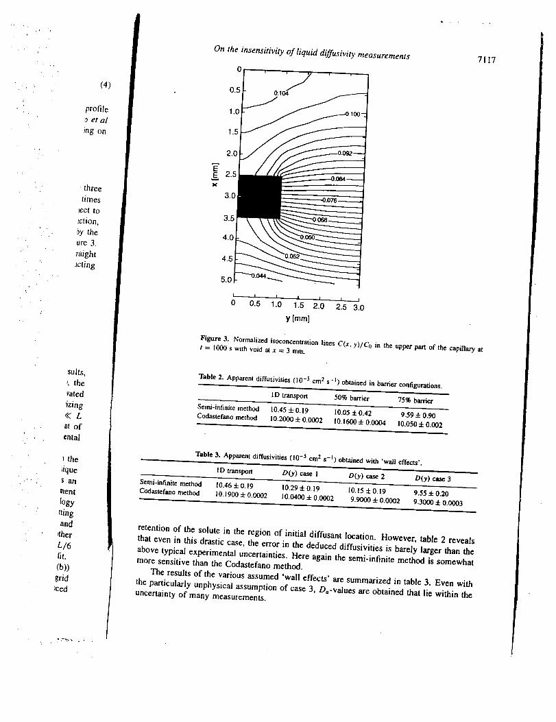
profile

aet al

ing on

!three

times

_cci {o

_ction,

., by the

ure 3.

raight

_cting

suits,

_, the

rated

Jzing

(<L

at of

cntal

the

_ique

. ' _ all

nent

Iogy

tting

and

Jther

L/6

fit.

(b))grid

Iced

EeX

On the insensitivity of liquid diffusivity measurements

0

0.5

I I I I I

0.5 1.0 1.5 2.0 2.5 3.0

y [mm]

Figure 3. Normalized isoconcentration lines C(x, y)/C_ in the upper part of the capillary att = 1000 s with void at x = 3 ram.

7117

Table 2. Apparent diffusivities (10-5 cm 2 s-I) obtained in barrier configurations.

ID transport 50% barrier 75% barrier

Semi-infinite method 10.45 + 0.19 10.05 4- 0.42 9.59 4- 0.90

Codastefano method 10.2000 4- 0.0002 10,1600 4- 0.0004 10.050 4- 0.002

Table 3. Apparent diffusivities (10-5 cm 2 s-I) obtained with 'wall effects'.

ID transport D(y) case 1 D(y) case 2 D(y) case 3

Semi-infinite method 10.464-0.19 10.294-0.19 10.154-0.19 9.554-0.20

Codastefano method 10.1900 4- 0.0002 I0.0400 4- 0.0002 9.9000 4- 0.0002 9.3000 4- 0.0003

retention of the solute in the region of initial diffusant location. However, table 2 reveals

that even in this drastic case, the error in the deduced diffusivities is barely larger than the

above typical experimental uncertainties. Here again the semi-infinite method is somewhatmore sensitive than the Codastefano method.

The results of the various assumed 'wall effects' are summarized in table 3. Even with

the particularly unphysical assumption of case 3, Do-values are obtained that lie within theuncertainty of many measurements.

7118 L B Jalbert et al

0.11

0.1,

0.1'

0.1,

cYx_- 0.0_

U

0.06

0.04

0.02

0

.... i .... i .... i .... i .... ! ....

t = 1,000 S

t = 2,000 s• N.

= 10,000 s

.... t .... "'te..F...,___-_-._,._ , ,.. ,, i ....5 10 15 20 25 30

x [mm]

Figure 4. Normalized concentration profiles at three diffusion times. Full curves, with 75%

barrier at x = I mm; broken curves, unobstructed diffusion.

Table 4. Maximum normalized radial concentration variation at x = L/6.

Case Radial AC/C (%) Time of occurrence (s)

D(y) case I 0.014 250

D(y) case 2 0.028 230

D(y) case 3 0.082 230

The insensitivity of the concentration distribution to postulated 'wall effects' is further

illustrated in figure 5, in which we have plotted the concentration difference (normalized

to the samples maximum C) between case 3 and the ID transport result at 300 s. It is

evident that solute redistribution by radial diffusion prevents the formation of significant

concentration gradients across the width of the sample. This is also supported by the low

values of the maximum radial concentration variation at position x = L/6 listed in table 4.

Note that these maxima occur early in the diffusion runs. Thus they are unlikely to be

detectable in diffusivity measurements. As a consequence, experimental findings of radial

concentration gradients in cylindrical diffusion samples indicate convective contamination

(for detailed examples see [12]) rather than inferred dependences of diffusivity on thedistance from the container wall.

4. Conclusions

The above 2D simulations show that the influence of the model voids, barriers and 'wall

effects' on concentration distributions in diffusion samples and the subsequently deduced

diffusivities is rather marginal. Note that in real, 3D systems, owing to the lower cross-

sectional fraction taken on by such obstacles of the same radial dimensions, the deviations

from unobstructed diffusive transport will be even less significant. Hence, we conclude that

the contamination of diffusivity measurements owing to such geometrical parameters will in

, p,

!

On the insensitivity of liquid diffusivity measurements

0

7119

E

X

6

9

I I I I

0 0.5 1.0 1.5

y[mm]

Figure 5. Difference in concentration between the 'wall effect' case 3 and uniform diffusion,AC(x, y), normalized to the maximum concentration, obtained in the top part of the sample att = 300 s. Numbers in 10-2%.

most cases be negligible compared with the convective contamination arising from sample

non-isothermality [ 12].

Acknowledgments

This research has been supported by the National Aeronautics and Space Administration

under contract NCC8-99, and by the State of Alabama through the Center for Microgravity

and Materials Research at the University of Alabama in Huntsville. We are much obliged

to J I D Alexander for advice on the use of the CFD code.

References

[1] Pollman K W, Stodieck L S and Luttges M W 1994 Microgravity Sci. Tech. 7 50

[2] Weinberg F and Mui C 1994 Can. Metal. Quart. 33 233

[3] Careri G, Paoletti A and Vinccntini M 1958 Nuovo C_mento 10 1088

14] Foster J P and Reynik R J 1973 Met. Trans. 4 207

[5] Nachtrieb N H 1967 Proc. Int. Conf. on Properties in Liquid Metals ed P D Adams, H A Davies and

S G Epstein (London: Taylor and Francis) p 309

16] Crank J 1956 The Mathematics of Diffusion (Oxford: Clarendon)[7] Codastefano P, Di Russo A and Zanza V 1977 Rev. Sci. Instrura. 48 1650

7120 L B Jalbert et al

[8] Jalbert L B, Banish R M and Rosenberger F 1998 Phys, Rev. E 57 1727

[9] Lodding V A 1956 Z. Natuq_ a 11 200

[10] Nachtrieb N H 1976 Berichte Bunsenges. 80 678

[I 1] Simoji M and Itami T 1986 Atomic Tran.rporl in Liquid Metals (Aedermansdorf, Switzerland: Trans. Tech.)

[12] Alexander J I D, Ramus J-F and Rosenberger F 1996 Micrograviry Sci. Tech. 9 158

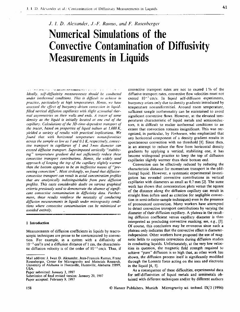
.I.I. 1). Alexander ct al.: Contaminati,ml of I)iffusivltv Mcasure,ncnts in Liquids 41

J. I. D. Alexander, J.-F. Ramus, and F. Rosenberger

Numerical Simulations of theConvective Contaminationof DiffusivityMeasurementsin Liquids

Ideally, self-diffusivity measurements shouM be comhlctedunder isothermal conditions. This is difficult to achieve in

practice, particularly at high temperatures. Hence, we haveassessed the effect of buoyancy-driven convection in liquid-filled vertical diffusion capillaries with slight azimuthal ther-mal asymmetries on their walls and ends. A tracer of samedensity as the liquid is initially located at one end of thecapillary. Calculations of the 3D-time-dependent transport ofthe tracer, based on properties of liquid indium at I,O00 K,yielded a variety of results with practical implications. Wefound that with horizontal temperature nonuniformitiesacross the sample as log, as 1 and O.1 K, respectively, convec-tive transport in capillaries of 1 and 3ram diameter canexceed diffusive transport. Superimposed vertically "stabiliz-ing" temperature gradient did not sufficiently reduce theseconvective transport contributions. Hence, the widely usedapproach of keeping the top of the capillary slightly warmerthan the bottom appears to be an ineffective means of "pre-venting convection". Most strikingly, we found that diffusive-

convective transport can result in axial concentration profilesthat are analytically indistinguishable from pure diffusionprofiles. This casts considerable doubt on various graphicalcriteria previously used to demonstrate the absence of signifi-cant convective contamination in diffusivity data• Further-more, these results reinforce the necessity of conductingdiffusion measur'ements in liquids under microgravity condi-tions where convective contamination can be minimized or

avoided entirely.

1 Introduction

Measurements of diffusion coefficients in liquids by macro-

scopic techniques are prone to be contaminated by convec-tion. For example, in a system with a diffusivity of10 -5 cm2/s and a diffusion distance of 1 cm, the characteris-tic diffusion velocity is of the order of i0 -s cm/s. Thus, if

Mail address: J. Iwan D. Alexander, Jean-Francois Ramus, FranzRosenberger, Center for Microgravity and Materials Research,University of Alabama in Huntsville, Huntsville, Alabama 35899,USA.Paper submitted: January 3, 1997Submission of final revised Version: January 20, 1997Paper accepted: February 9, 1997

convective transport rates are not to exceed 1% of thediffusive transport rates, convective flow velocities must notexceed 10-7cm/s. In liquid self-diffusion experiments,buoyancy arises only due to density gradients introduced by

temperature nonuniformitieL Around room temperature,sufficient sample isothermality can be maintained to avoidsignificant convective flows. However, at the elevated tem-peratures characteristic of liquid metals and semiconduc-tors, it is difficult to realize isothermal conditions to anextent that convection remains insignificant. This was rec-

ognized, in particular, by Verhoeven, who emphasized thatany horizontal component of a density gradient results inspontaneous convection with no threshold [I]. Since then,in an attempt to reduce the flow from horizontal densitygradients by applying a vertical, stabilizing one, it has

become widespread practice to keep the top of diffusioncapillaries slightly warmer than their bottom end.

Convection can be effectively reduced by reducing thecharacteristic distance for momentum transport in the (dif-fusing) liquid. However, a systematic experimental investi-gation has revealed convective contributions in verticalcapillaries with diameters as small as 0.7 mm [2]. The same

work has shown that concentration plots versus the squareof the distance along the diffusion capillary can result instraight lines (often used as criterion for negligible convec-tion in semi-infinite-sample techniques) even in the presence

of pronounced convection. Many workers have attemptedto detect convective transport contributions by varying the

diameter of their diffusion capillary. A plateau in the result-ing diffusion coefficient versus capillary diameter is theninterpreted as precluding convective masking; see, e.g., [3].Of course, this conclusion may be erroneous since such aplateau only indicates that the convective effect is diameter-

independent. Other workers have proposed the use of mag-netic fields to suppress convection during diffusion studiesin conducting liquids. Unfortunately, at the very low veloc-ities in question, the magnetic field strength required toachieve "pure" diffusion is so high that, as other work hasshown, the diffusion process itself is significantly modified

through the Lorentz force acting on the ions and electronsin the liquid [4, 5].

As a consequence of these difficulties, experimental data

for self-diffusivities of liquid metals and semimetals ob-tained with different techniques and/or by different authors

158 © Hanser Publishers, Munich Microgravity sci. technol. IX/3 (1996)

.I.I.D. Alcxm,der c| al.: Contamination of Diffusivity Measurements in Liquids

":-_. _E80 Fig. I. Model d[ffusion Cal,illary.Tracer initially located in shaded layer

of thickness 3

typically differ by several 10%, and sometimes by more

than 100% [6, 7]. This is not only an obstacle to realistic

process modeling, but to our theoretical understanding of

diffusion in liquids as well. Although various theories exist

for the diffusion in liquid elements and its tempera-

ture dependence, the uncertainties associated with most

diffusivity data are too large to allow for an unambiguousevaluation of these theoretical models. Currently, the differ-

ences .between .,several theoretical predictions are often less

• than those between different sets of data for the same

system.

To provide quantitative guidance for experimental work,

we have numerically modeled diffusive-convective transport

in vertical cylinders with dimensions typical for diffusion

experiment geometries. To account for thermal convective

transport contributions we imposed slight azimuthal tem-

perature asymmetries on the walls and ends of these capil-

laries. A diffusant, representing the isotopic tracer used in

the self-diffusion experiments, is initially located at one end

of the capillary. The 3D-time-dependent transport of the

diffusant was then simulated for physical properties corre-

sponding to liquid indium. In the following, we present the

simulation model, the numerical approach, and the simula-

tion ' results together with their practical consequences.

2 Simulation Model

The liquid was assumed to be a Boussinesq fluid contained

in a closed vertical circular cylinder of length L = 30 mm

and diameter 2R (see fig. I) of 1 or 3 mm. Gravity acts

along the cylinder axis. The temperature on the vertical

cylinder wall has the form T(R, O, z) = (T_ + 7"2)/2 + (T_ -

T2)(cos(O))/2 + zlT_.z/L. Here Ti- 7"2= ,JT, is the maxi-

mum horizontal temperature difference across the cylinder

at any height z, and AT. is the temperature difference

between the colder bottom and warmer top faces. The

temperatures of these end faces are T(r, O, O) = (Ta + 7"_,)/2

+(T t - T2)r(cos (O))/(2R) and T(r, O, L) = T(r, O, O) +

J 7".., respectively. The imposed temperature gradients are

time-independent. From this, and their assumed small mag-

nitude, we expect the resulting flow to be steady. Hence, for

given values of J To, J T., and R we can compute a steady

solution to the following mass, momentum, and heat trans-

port equations:

divu+0, (I)

1u • grad u = -- Vp + v Au - fl(T - T2)gk, (2)

0

u • grad T = _: A 7". (3)

Here u, T, Oo, fl, v, and x are the liquid's velocity, tempera-

ture, density, thermal expansion coefficient, kinematic vis-

cosity, and thermal diffusivity, respectively. Note that, since

we consider self-diffusion experiments for which the tracer

density is equal to the density of the host liquid, there are

no solutal contributions to buoyancy. The no-slip condition

for velocity is applied at all walls. Having found the steady

velocity and temperature distributions we then use u to

compute the evolution of the concentration field c(x, t)

from

_c

_-_ + u • grad c = D Ac, (4)

where D is the self-diffusivity. As indicated in fig. 1, the

diffusant (tracer) is initially located in a thin layer of

thickness 8 at one end of the capillary. Hence, the initial

concentration distribution is

c(z,O)=co, O<z<6 and c(z,O)=O, O<z<_L, (5)

where 6/L << 1. No flux of the tracer is permitted through

the walls and ends of the capillary.

The simulations were carried out using the physical

properties of molten indium evaluated at T= 1,000 K

(table 1) together with an assumed diffusjvity of 1.48.

10 -5 cm2/s. Since it is desirable to measure self-diffusion

coefficients over a wide temperature range, we have evalu-

ated the relevant properties also at lower temperatures. One

sees from table 1 that, in particular, the viscosity varies

considerably with temperature. For an extrapolation of our

results to lower temperatures, the reader should multiply

the T = 1,000 K value of ,d To by the ratio given in the far

right column. For example, at 850 K, the convective contri-

Tabl_, .I Phy. ' p pricalro ertie_', pfoindium fior diiffierent temoeratures..... above the melting point (429K) calculated from data in [8, 9]. Thesimulations were carried out for properties corresponding to T = 1,000 K. To obtain the horizontal temperature difference, zl To, which, at thelower temperatures would give rise to the same flow as the 1,000 K case, multiply the zt To for 1,000 K by the ratio given in the last column

T

[KI

. 1,000850600429

6.646.74

6.917.03

V

[10 -_-cm 2" s-']

0.781.272.092.65

0.110.110.110.11

1.021.010.980.97

alTo(T)

a L, (_,000 K)

1.01.652.79

3.60

Microgravity sci. technol. IX/3 (1996) 159

J. I. D.Alexanderel al.: Contamination of Diffusivity Measurements in Liquids

r = 0.75 R _

Fig. 2. Defining sketch for data evaluation; fi_r details see text

butions observed at T = 1,000 K will occur for a A To value

which is 1.65 times the ATo at !,000 K.

The governing equations and boundary conditions for

the time-dependent transport of heat, mass, and momen-

tum in the system were solved using finite differences on an

equally spaced and a variably spaced mesh using the flow

analysis software CFD2000. With the latter method, spatialdiscretization is achieved using a finite volume technique

[10]. The PISO algorithm [11] is used to' couple the dis-

cretized heat and momenttim transport equations which

were solved using an ADI method [12]. Owing to the large

length to diameter ratio of the capillaries (20 and 60) we

found it necessary to employ 24 x 12 x 140 points in,the

azimuthal, radial, and axial directions, respectively.

3 Data Analysis and Presentation

Time histories of the tracer concentration fields were ob-

tained for different values of R, A T6, and ,6 T.. To assess

the consequences of the different temperature nonuniformi-ties for diffusion coefficient measurements, we treated each

of the calculated tracer time histories as we would experi-

mental data. Two approaches were used to deduce diffusiv-

ity values from the calculated concentration distributions.In the first approach we employed the method of Codaste-

fano et al. [13] in which time records of the concentrationct(t) and c2(t), respectively, at the axial sample locations

z = L/6 and 5L/6 are used to calculate the diffusivity D

from the relation

in [ct(t) - c2(t)] = const. - (n/L)2Dt. (6)

As indicated in fig: 2, the concentration values were taken

at the respective positions z as averages over either theentire cross-section (D = De) or over the ring-shaped re-

gion 0.75 <_r < R,O<O < 2n (D= Dw).

In the second approach we used the solution to the

following 1D diffusion problem for c(z, t)

_c D 02c (7)

Oc(0, t_____)= 0, t > 0, (8)0z

0<z<6, and c(z, 0)=0, 6<z<L, (9)c(z, O)= Co,

where 6 << L and c(:, t) is bounded as : _ ,_v. The solution

has the form [14]

c(z, t) = _----_t exp , (I(})

and D is obtained graphically from the slope m of

In (c('-, t)) versus :-' at t =/*, where m is given by

0In (c(:, t*)) -1 (111m = Oz 2 = -4Dt*"

In the second method we calculated three diffusivities from

the concentration profiles along the three vertical axes

represented by heavy lines in fig. 2. One value was obtainedfrom the axial concentration profile at r = 0 (D = D,,, ) and

the other two from axial profiles taken at r = 0.75R and

0=0and rt (D=Do_o,D=D ..... ) respectively.

4 Results and Discussion

The results of our simulations are summarized in table 2.

One sees that, irrespective of the application of a "stabiliz-

ing" A T_, with the I mm diameter capillary the horizontal

temperature difference A T0 must not exceed 0.1 K for the

apparent diffusivity D to be within a few percent of the

actual (input) diffusivity Do. However, at A T, = 1 K, which

we consider as a readily occurring temperature nonunifor-

mity for experiments at 1,000 K, Dc exceeds Do by over

100%. The magnitude of this convective contamination,

though somewhat reduced by the A T. of 2 K, fully demon-

strates the difficulty of accurately measuring diffusivities at

elevated temperatures in the presence of gravity. These

results are further illustrated in fig. 3a with time records for

c_ and c2 used in the Codastefano method, eq. (6). The

convective transport contributions become particularly ap-

parent when comparing the curves obtained with gravity

(heavy solid lines: d T.. = 0, dashed lines: AT: = 2 K) with

the thin solid line resulting under purely diffusive condi-

tions. On the other hand, the plots of in (c_ - c2), obtained

under these strongly contaminated conditions, are as

straight as one would expect for pure diffusion. Thus, the

' straight line character of these plots cannot be used as a

Table 2. Apparent diffusiuities in units of [10- J cm 2s - i] obtainedfrom the simulations with input diffusivity Do= 1.48" lO-_ cm zr- a. Values with * obtained at t = 300 rain, with ** at 356 rain

zJT,=OK 2R=l mm 2R=3mm

ATo [K] 1.0 0.1 0.01 0.1 0.05 0.01Dc 3.69 1.50 1.48 7.92 3.08 1.54Dw 3.69 1.50 1.48 7.92 3.08 1.54D_._ 2.25** 1.50" 1.51"* 7.87** 3.26* 1.60"Do._o 2.25"* 1.49" 1.49"* 6.18"* 2.75* 1.51"Dox,, 2.25** 1.49' 1.49"* 8.43** 3.45* 1.57'

zJL=2K

dTo [K] i.0 0.1 0.1 0.077 0.01D c 2.63 1.51* - 8.93 5.73 1.55

Dw 2.63 I.Sl* - 8.93 5.73 1.57D,, 2.25** 1.48' - 8.76** 7.02* 1.60'D,._o 2.25** 1.47" - 7.19"* 5.96* 1.51"D_._,, 2.25** 1.47" - 8.76** 7.64* 1.57"

160 Microgravity sci. technol. IX/3 (I 996)

._ I 1_ .\lt_'_,_L_,.tCl ct _d.: £otlt_tnutlattot_ of L)illusivily Mcasurcmcnts ttl Liqutds

f I I I I

f .8

@

° // /

0 l/ 1 _ _--'-"_'---'_"--q I0 100 200 300 400 500

Time [min]

-4.3_ r,.,. ] I _ =

It_"_""', DC = 2.63 x 10 "s em2/s

_"_ ATz=2 K

I

DC=3.

i5_ 5

/ x<I t I t i i

100 200 300 400 500

Time [min]

16X

o

z

-4

-5

O

I

-6

-7

I I I I

(a)

100 200 300 400 500

Time [min]

I I I I

N_D c = 7.92 x 10 .5 cm2/s

"_. (b)

Dc --8.93 x 10 "s cm2/s ",,,,_

ATz = J_ .2., ",,_

I I I I ]"

1O0 200 300 400 500

Time [min]

Fig. 3 (/eft). (a) Normalized average con-eentration cl (upper curves) and c, (lower

curves) vs time and (b) In (cl - c2) vs time,

.for 2R = l mm and z_Tr_= l K. The pure

diffusion case is shown for reference m (a).The solid and dashed lines correspond to

A T. = 0 and 2 K, respectively

Fig. 5. (right). (a) Normalized average con-

centration el (upper curves) and c_, (lower

curves) us time and (b) In (cl - cz) vs time,

for 2R = 3 mm and zJ To = O. 1 K. The pure

diffusion case is shown for reference in (a).

The solid affd "dashed lines correspond td

A T_ = 0 and 2 K, respectively.

criterion for the absence of significant convective contribu-

tions. More insight on the convective mixing in this casecan be obtained from the isoconcentration lines in the plane

0 = 0,/_ (fig. 4). The deformation of these lines, whichunder purely diffusive conditions would be strictly straightand horizontal reflects a convection role with the liquid

rising at the right ("hotter") wall and sinking at the leftwall. Characteristic convection velocities associated with

these rolls are of the order of 8 • 10 -4 cm/s. A comparisonof these concentration contours for ,_T= = 0 (solid line) and "

(a)

g

1,f..

.j..

.j.-

"_. 15 x 10 "3

..... _16.5 x 10 .3

(b)

tLT z = 0

.... - ..... AT z = 2 K

.-9.9 x 10 "a--_ "11.1 x 10 -3

Fig. 4. Normalized concentration contours for 2R = I mm and

AT,= I K at (a) t= 178 and (b) 356rain. Contour intervals: (a)5" 10-4; (h) 4. I0 -_

A T== 2 K (dashed lines) again illustrates the limited effectof the common practice to keep the top of the diffusioncapillary somewhat warmer in order to suppress convec-tion.

The results for 3 mm diameter capillaries are even more

sobering. Table 2 reveals that ATo's of a few 10-_ K sufficeto induce intolerable convection contamination. For the

case of A To = 0.1 K, the strong convective contributions

become apparent by comparing the plots of c_ and c_ in fig.5a with those in fig. 3a. One sees that in the wider capillarythe. concentration at the "Codastefano locations" (see

above) increases much more rapidly than in the _narrowercapillary. This is due to an increase of the convective

velocities to 7" 10 -_ cm/s. This increase is also reflected in

the stronger deformation of the isoconcentration lines,which are presented in fig. 6 for this case. In:spite of thisheavy convective contamination, the linearity of theIn (c_ - c_) versus time curves at large times (flg. 5b) mightagain lead one to erroneously conclude that convection isinsignificant! Equally interesting is the result that A T_ =2 K, rather than reducing the flow induced by A Ta, slightlyenhances the convective contribution. We have' observed asimilar behavior associated with transport during Bridg-

man-Stockbarger solidification under microgravity condi-

tions [15].The above discussionwas restricted to D-values ob-

tained by the Codastefano method, eq. (6). The apparentdiffusivities obtained by the second method, eq. (10), reflecta similar behavior. Despite the obvious convective contam-inations, plots of the logarithm of the concentration versusthe square of the distance along the diffusion capillary(which are employed in this method for D-evaluations, see

Microgravity sci. technol. IX/3 (1996) 161

J I. I). Alexander cl al.: Coutamiualion of Diffusivily Meastnements in Liquids

I--_.--- (a)

' / /7

,'1 ,'f t9

////>8.5 × 10 .3

Fig. 6. Normali:ed

," (b)

-- ATz= 0ATz= 2 K

_ _ 6.4 x 10 3

conc£,nltaflon ('Oltfaal's

/br 2R= 3mm and `3T,=O. I K at (a) t=178 and (b) 356min. Contour intert,als: (a)

I0-': (b) 4" 10-"

0

-5.0

-5.5

-6.(I

-6._0

i I I l I I I I

I I [ I I I I I

2 4 6 8

z=[cm21

Fig. 7. Plots of h_ c vs z-" ahmg the threeaxis &:fined m fig. 2. Sanle sample as m figs.3 and 4: 2R = l mm and ,3T, = I K, ,3T. =

O, at t = 356 rain. Dashed straight line: guideJbr the eye to emphasize ahsence of curva-ture m pro[lies over large parts _tf the sample

"5 _,Da xu -6

-7 Dax0 __,_

8 , , , ....0 2 4 6 8

z= [cm 2]

Fig. 8. Plots as .fig. 7 sam�des as ir /igs. 5and 6: 2R = 3mm and ,3T,= O. I K, AT_=

O, at t = 356 rain

eq. (11)) result in rather straight lines over major portions

of the sample. This is depicted in figs. 7 and 8, respectively,

for the ,JT:=0 cases of figs. 3 and 5. Typical liquid

diffusivity studies involve the solidification of the sample

before the chemical analysis for c(z) determination. This

solidification often results in high porosity or deformation

of the last part of the sample to freeze. On discarding this

part of the sample, an investigator would again reach theerroneous conclusion that convective contamination was

insignificant. • .. e

5 Summary and Conclusion

We found that temperature nonuniformities of magnitudes

that, in particular at high temperatures, are practically

unavoidable during diffusivity measurements in liquids,

cause strong convective contamination of the diffusivitydata. Furthermore, the convective contribution to transport

is only insignificantly reduced by a "stabilizing" A_.

Hence, the widely used approach of keeping the top of

diffusion _amples slightly warmer than the bottom appears

to be a dubious means of "preventing convection". Most

strikingly, we found that diffusive-convective transport canresult in temporal local concentration changes and axial

concentration profiles that are analytically indistinguishable

from pure diffusion profiles. This finding casts considerable

doubt on various geometrical criteria previously used todemonstrate the absence of significant convective contami-

nation in diffusivity data plots.From this study we conclude that reduced gravity condi-

tions are essential for definitive diffusivity measurements in

liquid phases of macroscopic dimensions.

Acknowledgments

This work has been supported by the Microgravity Science andApplication Division of the National Aeronautics and Space Ad-ministration under contract NAS8-39716 and grant NCC8-99, and

by the State of Alabama through the Alabama SupercomputerNetwork and the Center for Microgravity and Materials Research

at the University of Alabama in Huntsville.

References

1 Verhoeven, J. D.: Convection Effects in the Capillary ReservoirTechnique for Measuring Liquid Metal Diffusion Coefficients.Trans. Met. Soc. AIME, vol. 242, p. 1937 (1968)

2 Persson, T., Erikson, P. E., Linstr6m, L.: Convection and Other

Disturbing Effects in Diffusion Experiments in Liquid Metals.J: Physique, vol. 41, p. C8-374 (1980)

3 Careri, G., Paoletti, A. and Saloetti, F.: Self-diffusion in LiquidIndium. Nuovo Cimento, vol. 10, p. 399 (1954)

"4 Youdelis, W. V., Colton, D. R., Cahoon, J. R.: On the Theoryof Diffusion in a Magnetic Field. Can. J. Phys., vol. 42, p. 2217

(1964)5 Youdelis, W. V., Colton, D. R., Cahoon, J. R.: Diffusion in a

Magnetic Field. Ca_= J. Phys., vol. 48, p. 805 (1970)6 Shimoji, M., hami, 7".: Atomic Transport in Liquid Metals.

Trans. Tech. Publ., Aedermannsdorf, Switzerland (1986)7 March, N. H.: Liquid Metals - Concepts and Theory. Cam-

bridge Univ. Press, Cambridge (1990)8 Ida, T., Guthrie, R. L L.: The Physical Properties of Liquid

Metals. Clarendon, Oxford (1988)

9 Lind, M. D.: Thermocapillary Flows and Float Zone Processes.AIAA-Paper 87-0618, 25th Aerospace Sciences Meeting, RenoNV (1987)

10 Patankar, S. V.: Numerical Heat Transfer and Fluid Flow.Series in Computational Methods in Applied Mechanics andThermal Sciences, Hemisphere, London (1980)

11 lssa, R. I.: Solution of the Implicit Discretized Fluid FlowEquations by Operator Splitting. J. Comput. Phys., vol. 62, p.

40 (1985)12 Birkh¢_ G., Lynch, R.: Numerical Solution.of Elliptic Prob-

lems. SIAM Studies in Applied Mathematics (1984)

13 Codastefano, P., Di Russo, A., Zanza, V.: New Apparatus forAccurate Diffusion Measurements in Fluids. Rev. Sci. Instr.,

vol. 48, p. 1650 (1977)14 Crank, J.: The Mathematics of Diffusion. Clarendon Press,

Oxford, p. 13 (1975)15 Alexander, J. I. D., Ouazzani, J., Rosenberger, F.: Analysis of

the Low Gravity Tolerance of Bridgman-Stockbarger CrystalGrowth. J. Crystal Growth, vol. 97, p. 285 (1989)

162 Microgravity sci. technol. IX/3 (1996)