filmwise condensation over a tier of sphere a …etd.lib.metu.edu.tr/upload/12607923/index.pdf ·...
TRANSCRIPT
FILMWISE CONDENSATION OVER A TIER OF SPHERE
A THESIS SUBMITTED TO THE GRADUATE SCHOOL OF NATURAL AND APPLIED SCIENCES
OF MIDDLE EAST TECHNICAL UNIVERSITY
BY
TAMER ÇOBANOĞLU
IN PARTIAL FULFILLMENT OF THE REQUIREMENTS
FOR THE DEGREE OF MASTER OF SCIENCE
IN MECHANICAL ENGINEERING
DECEMBER 2006

Approval of the Graduate School of Natural and Applied Sciences
_____________________ Prof. Dr. Canan ÖZGEN
Director I certify that this thesis satisfies all the requirements as a thesis for the degree of Master of Science.
_____________________ Prof. Dr. S. Kemal İDER
Head of Department This is to certify that we have read this thesis and that in our opinion it is fully adequate, in scope and quality, as a thesis for the degree of Master of Science.
_____________________ Assoc. Prof. Dr. Cemil YAMALI
Supervisor Examining Committee Members Prof. Dr. Faruk ARINÇ (METU,ME) _____________________ Assoc. Prof. Dr. Cemil YAMALI (Affiliation) _____________________ Prof. Dr. Kahraman ALBAYRAK (Affiliation) _____________________ Asst. Prof. Dr. Tahsin ÇETİNKAYA (Affiliation) _____________________ Asst. Prof. Dr. İbrahim ATILGAN (GAZI UNIV.) _____________________

iii
I hereby declare that all information in this document has been obtained and presented in accordance with academic rules and ethical conduct. I also declare that, as required by these rules and conduct, I have fully cited and referenced all material and results that are not original to this work.
Name, Last name :
Signature :

iv
ABSTRACT
FILMWISE CONDENSATION OVER A TIER OF SPHERE
ÇOBANOĞLU, Tamer
M.S., Department of Mechanical Engineering
Supervisor:Assoc. Prof. Dr.Cemil YAMALI
December 2006 , 131 pages
The objective of this study is to determine the mean heat transfer coefficient
and heat transfer rate and to analyse the effect of inclination angles,the effect
of subcooling temperatures and the effect of vapour velocity for laminar
filmwise condensation of water vapour on a vertical tier of spheres
experimentaly and analyticaly. For this purpose, the experimental aparatus
were designed and manufactured. In the free condensation experimental
study Ø50mm and Ø60 mm O.D. spheres were used to analyse the
diameter effect . In the experimental studies of free and forced condensation
Ø60mm O.D. spheres on which vapour flows at 2,75 bars were used to
analyse the effect of vapour velocity. For the experimental study of the
annular condensation in the concentric spheres the effect of vapour velocity

v
was studied by forcing the vapour to flow in the area between two concentric
spheres.
In the free condensation experiments it is observed that at smaller diameters
the heat flux and mean heat transfer coefficients for sphere is higher. In the
free and forced condensation experiments increasing the velocity of vapour
increases the mean heat transfer coefficient. At the experiments with annular
condensation between the concentric spheres high mean heat transfer
coefficient values have been obtained compared to the free and forced
condansation over the surface of spheres experimental studies.
Keywords: Laminar, film condensation, sphere, inclination angle, forced
condensation.

vi
ÖZ
DİKEY SIRALANMIŞ KÜRELER ÜZERİNDEN
FİLM YOĞUŞMASININ İNCELENMESİ
ÇOBANOĞLU , Tamer
Y.Lisans, Makine Mühendisliği Bölümü
Tez Yöneticisi: Doç. Dr.Cemil YAMALI
Aralık 2006 , 131 sayfa
Bu çalışmanın amacı, deneysel ve analitik yöntemler kullanılarak, dikey
sıralanmış küreler üzerinden akan su buharının laminar yoğuşması
esnasında gerçekleşen ortalama ısı transfer katsayılarının hesaplanması ve
buhar hızı, eğim açısı ile buhar ve yüzey sıcaklık farkı etkisinin analiz
edilmesidir. Bu amaç için, bir deney seti tasarlanarak imal edilmiştir. Deneyler
3 aşamalı olarak gerçekleştirilmiştir. Serbest yoğuşma deneyinde, Ø50mm ve
Ø60mm çaplarında küreler kullanılarak çap etkisi incelenmiştir. Serbest ve
zorlanmış yoğuşma deneyinde üzerinden 2,75 bar buhar akan Ø60mm
küreler kullanılarak, durağan ve hızlı akan buhar etkisi incelenmiştir. İç içe
geçirilmiş eş merkezli iki küre deneyinde serbest ve zorlanmış yoğuşma etkisi
incelenmiştir.

vii
Serbest yoğuşma deneyi sonucunda küçük çaplı kürede ortalama ısı transferi
katsayısının daha yüksek çıktığı görülmektedir. Serbest ve zorlamalı
yoğuşma deneyi sonucunda yüksek buhar hızlarında film kalınlığının düştüğü
ve ortalama ısı transferi katsayısının yükseldiği görülmektedir. İç içe
geçirilmiş eşmerkezli küreler deneyinde elde edilen ortalama ısı transferi
katsayılarının diğer deneylerde elde edilen değerlerden daha yüksek çıktığı
görülmektedir.
Anahtar kelimeler: Laminar, film yoğuşması,küre, tırmanma açısı, hızlı buhar.

viii
ACKNOWLEGEMENTS
I would like to thank my supervisor, Assoc. Prof. Dr. Cemil YAMALI for his
continuous guidance, support and valuable contribution throughout this
study. I gratefully acknowledge Cengiz Akkor, Hükümdar Ertan and Hamdi
Genç for their technical assistance in manufacturing and operating the setup.
I am grateful to the jury members for their valuable contributions.
I express my deepest gratitude to my mother Gülsüm Çobanoğlu, my father
Fuat Çobanoğlu and my wife Ahsen Çobanoğlu for their encouragements
throughout my education life.
.
ix
TABLE OF CONTENTS
PLAGIARISM..................................................................................................iii
ABSTRACT.................................................................................................... iv
ÖZ..................................................................................................................vi
ACKNOWLEGEMENTS............................................................................... viii
TABLE OF CONTENTS................................................................................. ix
LIST OF TABLES......................................................................................... xiii
LIST OF FIGURES ...................................................................................... xiv
LIST OF SYMBOLS ......................................................................................xx
CHAPTER...................................................................................................... 1
1. INTRODUCTION.................................................................................... 1
1.1 Condensation................................................................................... 1
1.1.1 Filmwise Condensation ............................................................ 1
1.1.2 Dropwise Condensation ........................................................... 2
1.2 Condensate Film Structure .............................................................. 2
1.3 Effects of Non-Condensable Gases................................................. 3
1.3.1 Stationary Vapor with a Noncondensable Gas......................... 3
1.3.2 Moving Vapor with a Noncondensable Gas ............................. 4
1.4 Laminar and Turbulent Flow ............................................................ 4
2. REVIEW OF PREVIOUS STUDIES ....................................................... 7
3. ANALYTICAL MODEL...........................................................................16
3.1 Assumptions ...................................................................................16
3.2 Physical Model................................................................................17
3.3 Formulation of the Problem.............................................................18
3.3.1 Velocity Profile.........................................................................18
3.3.2 Conservation of Mass..............................................................18
3.3.3 Conservation of Momentum ....................................................21

x
3.3.4 Heat Transfer Equation ...........................................................22
3.4 Calculation of the Initial Values.......................................................22
3.5 Finite Difference Equations.............................................................24
3.6 Calculation for the Lower Spheres ..................................................26
4. EXPERIMENTAL STUDIES ..................................................................30
4.1 Case-1 Free Condensation Experimental Study.............................31
4.2 Case-2 Free and Forced Condensation Experimental Study..........31
4.3 Case-3 Annular Condensation in Concentric Spheres....................32
4.4 Experimental Setup ........................................................................32
4.5 Cooling Water Tank .......................................................................35
4.6 Boiler Tank......................................................................................36
4.7 Test Section....................................................................................37
4.7.1 Test Section Body ...................................................................38
4.7.2 Upper And Lower Caps ...........................................................41
4.8 Spheres ..........................................................................................42
4.8.1 First type of sphere:.................................................................42
4.8.2 Sphere used in the Free&Forced Condensation Experiments 45
4.9 Vapour Accelerater for Free&Forced Condensation Experiments ..48
4.10 Vapour Accelerater for Annular Condensation in Concentric........48
Spheres ........................................................................................48
4.11 Stainless Steel Pipe Connectors for thr Spheres ..........................49
4.11.1 Tight Fit Type of Pipe ............................................................49
4.11.2 Threaded Type of Pipe..........................................................50
4.12 Cooling Water Distributer Apparatus.............................................51
4.13 Pressure Reading System ............................................................53
4.14 Temperature Reading System ......................................................54
4.15 Thermocouple Layout ...................................................................55
4.15.1 Case-1:Free Condensation Experiment ................................55
4.15.2 Case-2:Free&Forced Condensation Experiments .................56
4.15.3 Case-3:Annular Condensation in Concentric Spheres
Experiment ............................................................................57
4.16 Data Collecting Method.................................................................59

xi
4.17 Thermometer Calibration ..............................................................59
4.18 Experimental Procedure ...............................................................60
4.18.1 Mass Flow Rate Measurements For Case-1,
Case-2 & Case-3...................................................................60
4.18.2 Case-1 Free Condensation Experiments ..............................61
4.18.3 Case:2 Free&Forced Condensation Experiments .................61
4.18.4 Case:3 Annular Condensation in the Concentric Spheres ....62
5. RESULTS AND DISCUSSION..............................................................63
5.1 Experimental Results ......................................................................63
5.1.1 Case 1- Free Condensation Experiments ...............................64
5.1.2 Comparison of the Results of Ø50mm and Ø60mm Spheres .69
5.1.3 Case2 Free&Forced Condensation Experiments ....................74
5.1.4 Comparison of Free And Forced Condensation for Case-2 ....80
5.1.5 Case 3 Annular Condensation in the Concentric Spheres ......83
5.1.6 Comparison of Free and Forced Condensation for Case-3.....85
5.1.7 Effect of Wall Temperature......................................................87
5.1.8 Effect of Subcooling ................................................................87
5.1.9 Effect of Inclination Angle........................................................87
5.1.10 Effect of Sphere Diameter .....................................................88
5.1.11 Effect of Vapour Velocity .......................................................88
5.2 Analytical Results ...........................................................................88
5.3 Comparison of the Analytical and Experimental Studies ................92
5.4 Comparison of the Experimental Results with Literature ................94
5.5 Comparison of Sphere and Cylinder Results ..................................95
6. CONCLUSIONS ....................................................................................96
6.1 Discussion ......................................................................................96
6.2 Observations...................................................................................97
REFERENCES .............................................................................................99
APPENDICES.............................................................................................102
A. RESULTS OF THE FREE CONDENSATION EXPERIMENT ..........102

xii
B. RESULTS OF THE FREE&FORCED CONDENSATION
EXPERIMENTS ...............................................................................110
C. RESULTS OF THE ANNULAR CONDENSATION IN THE
CONCENTRIC SPHERES EXPERIMENT.......................................116
D. MATHCAD PROGRAM SOURCE....................................................118

xiii
LIST OF TABLES
TABLES
Table A.1 Experimental Results for 0o Inclination Angle, D=Ø60mm. ........102
Table A.2 Experimental Results for 12o Inclination Angle, D=Ø60mm. .......103
Table A.3 Experimental Results for 20o Inclination Angle, D=Ø60mm. ......104
Table A.4 Experimental Results for 30o Inclination Angle,D=Ø60mm. .......105
Table A.5 Experimental Results for 0o of Inclination Angle,D=Ø50mm. .....106
Table A.6 Experimental Results for 12o of Inclination Angle,D=Ø50mm. ...107
Table A.7 Experimental Results for 20o of Inclination Angle,D=Ø50mm. ...108
Table A.8 Experimental Results for 30o of Inclination Angle,D=Ø50mm. ...109
Table B.1 Experimental Results for 0o Inclination Angle,D=Ø60mm. .........110
Table B.2 Experimental Results for 5o Inclination Angle,D=Ø60mm. .........111
Table B.3 Experimental Results for 10o Inclination Angle,D=Ø60mm. .......112
Table B.4 Experimental Results for 15o Inclination Angle,D=Ø60mm. .......113
Table B.5 Experimental Results for 20o Inclination Angle,D=Ø60mm. .......114
Table B.6 Experimental Results of Forced Condensation for 0o Inclination115
Angle, D=Ø60mm. ....................................................................115
Table C.1 Experimental Results of Free Connvection for 0o
Inclination...................................................................................116
Table C.2 Experimental Results of Forced Connvection for 0o of
Inclination...................................................................................117
Tablo D.1 Values of Properties for Mathcad Program...............................118

xiv
LIST OF FIGURES
FIGURES
Figure 3.1 Physical Model and Coordinate System................................. 17
Figure 3.2 Differential Element and Energy Balance on the Liquid Film... 19
Figure 3.3 Flow Area and Heat Transfer Area on Differential Element...... 19
Figure 3.4 Physical Model for the Lower Spheres..................................... 27
Figure 4.1 General View of the Experimental Setup................................... 33
Figure 4.2 General View of the Free Condensation Experimental Setup.... 34
Figure 4.3 General View of the Free and Forced Condensation
Experimental Setup....................................................................
34
Figure 4.4 Technical Drawing of the Cooling Water Tank........................... 35
Figure 4.5 Technical Drawing of the Boiler Tank......................................... 37
Figure 4.6 Technical Drawing of the Test Section....................................... 39
Figure 4.7 Technical Drawing of the Test Section as Isometric View.......... 39
Figure 4.8 View of the Test Section After Manufacturing Processes.......... 40
Figure 4.9 View of the Test Section During the Test................................... 40
Figure 4.10 Technical Drawing of the Lower Cap...................................... 41
Figure 4.11 Technical Drawing of the Upper Cap...................................... 41
Figure 4.12 View of the Upper (left) and Lower (rigth) Caps....................... 42
Figure 4.13 Technical Drawing of the Shpere used in the Free
Condensation Experiments.....................................................
43
Figure 4.14 First Type of Spheres After Bonding and Polishing................ 44
Figure 4.15 First Type of Hemispheres and Inner Sphere......................... 44
Figure 4.16 The Placements of the First Type of Spheres in the
Test Section............................................................................
45
Figure 4.17 Technical Drawing of the Shpere used in the Free&Forced
Condensation Experiment.......................................................
46
xv
Figure 4.18 Shpere used in the Free&Forced Condensation Experiments
After Silver Welding and Polishing.........................................
46
Figure 4.19 Second Type of Spheres with Thermocouples........................ 47
Figure 4.20 The Placement of Second Type of Spheres in the Test
Section......................................................................................
47
Figure 4.21 The Placement of Vapour Accelerater for Free&Forced
Condensation Experiments......................................................
48
Figure 4.22 Drawing of the Vapour Accelerater for Case-3........................ 49
Figure 4.23 Technical Drawing of the Tight Fit Type of Pipe....................... 50
Figure 4.24 The View of the Tight Fit Type of Pipe..................................... 50
Figure 4.25 Technical Drawing of the Threaded Type of Pipe.................... 51
Figure 4.26 Technical Drawing of the Cooling Water Distributer
Apparatus, Bottom View. .........................................................
51
Figure 4.27 Technical Drawing of the Cooling Water Distributer
Apparatus, Front View..............................................................
52
Figure 4.28 View of the Cooling Water Distributer Apparatus.................... 53
Figure 4.29 View of the Pressure Reading System..................................... 54
Figure 4.30 View of the Temperature Reading System M3D12x................ 54
Figure 4.31 The Shematic View of the Thermocouple Layout for Free
Condensation Experimental Study..........................................
55
Figure 4.32 The Shematic View of the Thermocouple Layout for
Free&Forced Condensation Experimental Study....................
57
Figure 4.33 The Shematic View of the Thermocouple Layout for Annular
Condensation in Concentric Spheres Experimental Study......
58
Figure 5.1 Experimental Mass Flow Rate Variation with respect to Time
for Case-1, D=Ø60mm.............................................................
64
Figure 5.2 Variation of Heat Transfer Rate for 0o of Inclination for
Case1, D=Ø60mm...................................................................
65
Figure 5.3 Variation of Mean Heat Transfer Coefficient for 0o of
Inclination for Case-1, D=Ø60mm..........................................
65

xvi
Figure 5.4 Variation of Heat Transfer Rate for 12o of Inclination for
Case-1, D=Ø60mm....................................................................
66
Figure 5.5 Variation of Mean Heat Transfer Coefficient for 12o of
Inclination for Case-1, D=Ø60mm............................................
66
Figure 5.6 Variation of Heat Transfer Rate for 20o of Inclination for
Case-1, D=Ø60mm.....................................................................
67
Figure5.7 Variation of Mean Heat Transfer Coefficient for 20o of
Inclination for Case-1, D=Ø60mm..............................................
67
Figure 5.8 Variation of Heat Transfer Rate for 30o of Inclination for
Case-1, D=Ø60mm.....................................................................
68
Figure 5.9 Variation of Mean Heat Transfer Coefficient for 30o of
Inclination for Case-1, D=Ø60mm.............................................
68
Figure 5.10 Comparison of Heat Flux for 0o Inclination Angle for Upper
Sphere, D=Ø50mm and D=Ø60mm..............................................
69
Figure 5.11 Comparison of Heat Flux for 0o Inclination Angle for Middle
Sphere, D=Ø50mm and D=Ø60mm.........................................
70
Figure 5.12 Comparison of Heat Flux for 0o Inclination Angle for Bottom
Sphere, D=Ø50mm and D=Ø60mm.........................................
70
Figure 5.13 Comparison of Mean Heat Transfer Coefficient for 0o
Inclination Angle for Upper Sphere, D=Ø50mm and
D=Ø60mm...............................................................................
71
Figure 5.14 Comparison of Mean Heat Transfer Coefficient for 0o
Inclination Angle for Middle Sphere, D=Ø50mm and
D=Ø60mm...............................................................................
71
Figure 5.15 Comparison of Mean Heat Transfer Coefficient for 0o
Inclination Angle for Bottom Sphere, D=Ø50mm and
D=Ø60mm...............................................................................
72
Figure 5.16 Comparison of Mean Heat Transfer Coefficient for 12o
Inclination Angle for Upper Sphere, D=Ø50mm and
D=Ø60mm...............................................................................
72

xvii
Figure 5.17 Comparison of Mean Heat Transfer Coefficient for 12o
Inclination Angle for Middle Sphere, D=Ø50mm and
D=Ø60mm...............................................................................
73
Figure 5.18 Comparison of Mean Heat Transfer Coefficient for 12o
Inclination Angle for Bottom Sphere, D=Ø50mm and
D=Ø60mm...............................................................................
73
Figure 5.19 Experimental Mass Flow Rate Variation with respect to
Time for Free&Forced Condensation Experiments.................
74
Figure 5.20 Variation of Heat Transfer Rate for 0o of Inclination for
Case-2, Free Condensation...................................................
75
Figure 5.21 Variation of Mean Heat Transfer Coefficient for 0o of
Inclination for Case-2, Free Condensation............................
75
Figure 5.22 Variation of Heat Transfer Rate for 5o of Inclination for
Case-2, Free Condensation...................................................
76
Figure 5.23 Variation of Mean Heat Transfer Coefficient for 5o of
Inclination for Case-2, Free Condensation............................
76
Figure 5.24 Variation of Heat Transfer Rate for 10o of Inclination for
Case-2, Free Condensation...................................................
77
Figure 5.25 Variation of Mean Heat Transfer Coefficient for 10o of
Inclination for Case-2, Free Condensation............................
77
Figure 5.26 Variation of Heat Transfer Rate for 15o of Inclination for
Case-2, Free Condensation...................................................
78
Figure 5.27 Variation of Mean Heat Transfer Coefficient for 15o of
Inclination for Case-2, Free Condensation..............................
78
Figure 5.28 Variation of Heat Transfer Rate for 20o of Inclination for
Case-2, Free Condensation....................................................
79
Figure 5.29 Variation of Mean Heat Transfer Coefficient for 20o of
Inclination for Case-2, Free Condensation.............................
79
Figure 5.30 Comparison of Heat Transfer Rate for 0o of Inclination for
Case-2, Upper Sphere, Free and Forced Condensation.......
80
Figure 5.31 Comparison of Heat Transfer Rate for 0o of Inclination for
Case-2, Middle Sphere, Free and Forced Condensation.......
81

xviii
Figure 5.32 Comparison of Heat Transfer Rate for 0o of Inclination for
Case-2, Bottom Sphere, Free and Forced Condensation......
81
Figure 5.33 Comparison of Mean Heat Transfer Coefficients for 0o of
Inclination for Case-2,Upper Sphere, Free and Forced
Condensation.........................................................................
82
Figure 5.34 Comparison of Mean Heat Transfer Coefficients for 0o of
Inclination for Case-2,Middle Sphere, Free and Forced
Condensation.........................................................................
82
Figure 5.35 Comparison of Mean Heat Transfer Coefficients for 0o of
Inclination for Case-2,Bottom Sphere, Free and Forced
Condensation.........................................................................
83
Figure 5.36 Experimental Mass Flow Rate Variation with respect to
Time for Annular Condensation in Concentric Spheres.........
84
Figure 5.37 Variation of Mean Heat Transfer Rate for 0o of Inclination for
Annular Condensation in Concentric Spheres........................
84
Figure 5.38 Variation of Mean Heat Transfer Coefficient for 0o of
Inclination for Annular Condensation in Concentric
Spheres..................................................................................
85
Figure 5.39 Comparison of Heat Transfer Rate for Free and Forced
Condensation for Annular Condensation in Concentric
Spheres..................................................................................
86
Figure 5.40 Comparison of Mean Heat Transfer Coefficient for Free
and Forced Condensation for Annular Condensation in
Concentric Spheres................................................................
86
Figure 5.41 Variation of Film Thickness with Angular Position at
D=60mm and ∆T=8K.............................................................
90
Figure 5.42 Variation of Velocity of the Condensate with Angular
Position at D=60mm and ∆T=8K............................................
90
Figure 5.43 Variation of Heat Flux with Angular Position at D=60mm and
∆T=8K....................................................................................
91

xix
Figure 5.44 Variation of Heat Transfer Coefficient with Angular Position
at D=60mm and ∆T=8K.........................................................
91
Figure 5.45 Comparison of Mean Heat Transfer Coefficients for
Analytical and Experimental Studies for Upper Sphere.........
92
Figure 5.46 Comparison of Mean Heat Transfer Coefficients for
Analytical and Experimental Studies for Middle Sphere.........
93
Figure 5.47 Comparison of Mean Heat Transfer Coefficients for
Analytical and Experimental Studies for Bottom Sphere.......
93
Figure 5.48 Comparison of Mean Heat Transfer Coefficients Between
the Present Experimental Study and the Nusselt Analysis
for Sphere..............................................................................
94
Figure 5.49 Comparison of Mean Heat Transfer Coefficients Between
the Present Experimental Study and the Nusselt Analysis
for Cylinder...........................................................................
95

xx
LIST OF SYMBOLS
pC Specific heat at constant pressure, J/(kg.K)
g Gravitational acceleration, m/s2
h Convective heat transfer coefficient, W/(m2.K)
fgh Latent heat of condensation, J/kg
k Thermal conductivity, W/m.K
.
m Mass Flow Rate, kg/s
Pr Prandtl Number, k
C pµ
q Heat flux, W/m2
Q Heat transfer rate, W
T Temperature, K or CO
T1,…,T20 Thermocouples
t Time, s
A Area, m2
∆T Temperature difference, K
r Radius of the sphere, m
u x component of velocity, m/s
x Coordinate parallel to surface
y Coordinate normal to surface
xxi
Subscripts
cond Condensation
in Inlet
out Outlet
sat Saturation
w Wall
Greek Letters
δ Film thickness of the condensate layer, m
θ Angular position measured from the top of the sphere, rad.
µ Dynamic viscosity, kg/(m.s)
ρ Density, kg/m3
τ Shear stress, N/m2

1
CHAPTER 1
1 INTRODUCTION
1.1 Condensation
Condensation phenomena occur in many industrial
applications.Condensation is defined as the phase change from the vapor
state to the liquid or solid state. Condensation can occur on a solid surface or
in a bulk vapor. If the temperature of vapor is below its saturation
temperature according to its pressure it can take place in a bulk vapor. If the
temperature of the solid surface is below the saturation temperature of the
vapor condensation can occur on the solid surface. The subcooling condition
must be obtained for any type of condensation.
There are two idealized models of condensation, filmwise condensation and
dropwise condensation.
1.1.1 Filmwise Condensation
Filmwise condensation is the former and it occurs on a cooled surface which
is easily wetted. The vapor condenses in drops which grow by further
condensation and coalesce to form a film over the surface, if the surface-fluid
combination is wettable. Filmwise condensation is the most observed type of
cendensation. The removal of the film is the result of the gravity,
acceleration or other body forces.

2
Rates of heat transfer for film condensation can be predicted as a function of
bulk and surface temperatures, total bulk pressure, surface and liquid film
characteristics, bulk velocity and the presence of noncondensible gases.
Even though film condensation has been investigated extensively, the
majority of these studies were devoted to laminar film condensation (laminar
bulk flow and laminar film). Since the vapor flow in heat exchange equipment
may be turbulent, models and recent data are also reviewed for the
condensation flux with a turbulent mixture flow. A simple engineering
correlation or model is preferred many times for use in engineering design
studies and with existing computer system analyses.
1.1.2 Dropwise Condensation
Dropwise condensation occurs if the surface is non-wetting rivulets of liquid
flow away and new drops then begin to form. The phenomena of dropwise
condensation results in local heat transfer coefficients which are often an
order of magnitude greater than those for filmwise condensation. Even
though condensation phenomena can be classified into these categories of
dropwise and film condensation the initial period of condensation would
evolve into a film and probably would not affect the overall pressure-
temperature response unless drop condensation is promoted.
1.2 Condensate Film Structure
The condensate film characteristics depend on its flow field and the nature of
the condensing surface, e.g. roughness, wetting and orientation. Forced flow
induces interfacial instabilities that increase the heat transfer rates by
reducing the thickness of gas phase laminar sublayer and enhancing the
mixing of both the liquid (condensate film) and gas phase.
The surface finish has a major effect on the mode of condensation for a
downward facing surface and it is the wetting characteristics of the surface

3
that ultimately determine this. Dropwise condensation is likely to exist on
non-wetting surfaces and filmwise condensation is likely on wetting surfaces.
In dropwise condensation mode with polished metal surfaces, the heat
transfer characteristics are likely to change due to oxidation of the surface or
tarnishing. Thus, one cannot precisely know the wetting characteristics as
surface aging occurs.
1.3 Effects of Non-Condensable Gases
It can be observed that in actual cases some amount of non-condensable
gases occurs in the condensation system. In some systems such as steam
power plants because of the pressure less than atmospheric pressure air
leaking occurs in the convective flow. Also in some systems the dissolved
gases cause to occuring of non-condensable gases in the condensation such
as water and alcohol. When the condensing vapor carries non condensable
gases to the condenser surface, it acts as an empty area between the
condenser surface and the condensation of vapor. Therefore the heat
transfer comes to be difficult. So non-condensable gases reduce the heat
transfer rate both in filmwise and dropwise condensation.
1.3.1 Stationary Vapor with a Noncondensable Gas
A noncondensable gas can exist in a condensing environment and leads to a
significant reduction in heat transfer during condensation. A gas-vapor
boundary layer (e.g., air-steam) forms next to the condensate layer and the
partial pressures of gas and vapor vary through the boundary layer. The
buildup of noncondensable gas near the condensate film inhibits the diffusion
of the vapor from the bulk mixture to the liquid film and reduces the rate of
mass and energy transfer. Therefore, it is necessary to solve simultaneously
the conservation equations of mass, momentum and energy for both the
condensate film and the vapor-gas boundary layer together with the

4
conservation of specied for the vapor-gas layer. At the interface, a continuity
condition of mass, momentum and energy has to be satisfied.
1.3.2 Moving Vapor with a Noncondensable Gas
For a laminar vapor-gas mixture case, Sparrow, et al. (1967) solved the
conservation equations for the liquid film and the vapor-gas boundary layer
neglecting inertia and convection in the liquid layer and assuming the stream-
wise velocity component at the interface to be zero in the computation of the
velocity field in the vapor-gas boundary layer. Also a reference temperature
was used for the evaluation of properties. The results showed that the effect
of noncondensable gas for the moving vapor-gas mixture case is much less
than for the corresponding stationary vapor-gas mixture. A moving vapor-gas
mixture is considered to have a "sweeping" effect, thereby resulting in a
lower gas concentration at the interface (compared to the corresponding
stationary vapor-gas mixture case). Also, the ratio of the heat flux with a
noncondensable gas to that without a noncondensable gas was calculated to
be independent on the bulk velocity. The computed results reveal that
interfacial resistance has a negligible effect on the heat transfer and that
superheating has much less of an effect than in the corresponding free
condensation case.
1.4 Laminar and Turbulent Flow
Boundary layer is defined as the very thin layer in the intermediate
neighborhood of the body, in which the velocity gradient normal to the wall is
very large. In this region, the very small viscosity of the fluid exerts an
essential influence as the shearing stress may assume large values. At the
wall surface, the fluid particles adhere to it and the frictional forces between
the fluid layers retard the motion of the fluid within the boundary layer. In this
thin layer, the velocity of the fluid decreases from its free-stream value to
zero with no slip condition.

5
According to Prandtl, who intrctduced the boundary layer concept for the first
time, under certain conditions viscous forces are of importance only in the
immediate vicinity of a solid surface where velocity gradients are large. In
regions removed from the solid surface where there exists no large gradients
in fluid velocity, the fluid motion may be considered as frictionless, which is
called potential flow. In fact, there is no precise separating line between the
potential flow and boundary layer regions. However, boundary layer can be
defined as the region where the velocity component parallel to the surface is
less than 99% of the free-stream velocity.
An essential first step in the treatment of any flow problem is to determine
whether the flow is laminar or turbulent. Surface friction and the convection
transfer rates depend strongly on which of these conditions exists. There are
sharp differences between laminar and turbulent flow conditions. In the
laminar flow, fluid motion is highly ordered and it is possible to identify
streamlines along which particles move. Fluid motion along a streamline is
characterized by velocity components in both the x and y directions. Since
the velocity component v is in the direction normal to the surface, it can
contribute significantly to the transfer of momentum, energy or species
through the flow layers.
In contrast, fluid motion in the turbulent flow is highly irregular and is
characterized by velocity fluctuations. These fluctuations enhance the
transfer of momentum, energy and species, and hence increase surface
friction as well as convection transfer rates. Fluid mixing resulting from the
fluctuations makes turbulent flow layer thicknesses larger and flow layer
prdfiles (velocity, temperature and concentration) flatter than in laminar flow.
When the foregoing conditions for velocity distribution on a flat plate are
analyzed, it is seen that the flow is initially laminar, but at some distance from
the leading edge, small disturbances are amplified and transition to turbulent
flow begins to occur. Fluid fluctuations begin to develop in the transition

6
region, and the boundary layer eventually becomes completely turbulent. In
the fully turbulent region, conditions are characterized by a highly random,
three-dimensional motion of relatively large parcels of fluid, and it is not
surprising that the transition to turbulence is accompanied by significant
increases in the boundary layer thicknesses, the wall shear stress and the
convection coefficients.
In the turbulent flow, three different regions may be delineated. There is a
laminar sublayer in which transport is dominated by diffusion and the velocity
profile is nearly linear; there is an adjoining buffer layer in which diffusion and
turbulent mixing are comparable; and there is a turbulent zone in which
transport is dominated by turbulent mixing.
7
CHAPTER 2
2 REVIEW OF PREVIOUS STUDIES
In this section, the review of the literature with the theory background and
research findings will be presented. The review is mainly based on three
subjects: inclination angle, heat transfer, subcooling, film condensation,
laminar boundary layer and condensation on sphere & cylinder.
Michael Ming Chen [1] studied the cases of laminar film condensation over a
single and multiple horizontal tubes. In this analytical study neglecting the x-
component of vapor velocity outside the boundary layer and µvρv<<µρ were
assumed. Both the vapor boundary layer and the liquid film were considered
to be thin compared to the radius of the tube. All properties were taken
constant. Results: For single tube the temperature profiles are essentially the
same as the flat-plate case. The inertia forces have a larger effect on the
heat transfer of round tubes than flat plates. For vertical tubes the heat
transfer results for lower tubes were found to be consistently higher than
Nusselt’s theory. As a result of condensation between tubes a higher heat
transfer rate was predicted.
E.M.Sparrow and J.L.Gregg [2] studied the problem of laminar film
condensation on a vertical plate. In this analytical study energy-convection
and fluid-acceleration terms are fully considered. Solutions are obtained for
cp∆T / hfg between 0 and 2 for Prandtl numbers between 1 and 100.
Solutions are obtained both with and without acceleration terms. The addition

8
of acceleration terms introduces the Prandtl number as an additional
parameter. Negligible heat conduction across the liquid-vapor interface was
assumed. As a result it is found that the Prandtl number effect on the heat
transfer results is very small for high Prandtl numbers (Pr >1). So the effect
of Prandtl number on the heat transfer appears negligible for the range Pr >1.
The Pr=100 results are seen to coincide with those for no acceleration term.
But for lower Prandtl numbers, the acceleration terms should play a more
important role (Pr<1). As cp∆T / hfg increases, the inertia effects lead to a
dropping off of the Nusselt number.
Cz.O.Popiel and L.Boguslawski [3] studied the problem of heat transfer by
laminar film condensation on sphere surfaces taking into account liquid
wetting. Despite of horizontal tubes over sphere there was an influx of
additional condensate according to the change of the section area. The
neglecting of surface tensions was assumed. As a result of this study it was
seen that the average heat transfer coefficients on the upper and bottom
hemisphere surfaces are very close. The heat transfer coefficient decreases
slowly and then over the bottom hemisphere it decreases faster and faster as
it approaches the bottom stagnation point, in which it reaches zero. It is the
result of faster increase of the condensate thickness, caused by vapor
condensation, the decrease of the circumference, the condense flow down
and the tangential component of the gravity force.
V.H.Adams and P.J.Marto [4] analyzed the problem of laminar film
condensation on a horizontal elliptical tube in a pure saturated vapor for
conditions of free and forced condensation. They assumed the effects of
surface tension and pressure gradient in the condensate film. For free
condensation an elliptical tube with the major axis vertical showed an
improvement of nearly 11% in the mean heat-transfer coefficient when
compared to a circular tube of equivalent surface area. For forced
condensation with the same approach velocity as for a circular tube, a small
decrease (≈2%) in the mean heat-transfer coefficient resulted. However, for

9
the same pressure drop, heat transfer performance for an elliptical tube
increased by up to 16%. It can be seen that the effect of placing more of the
elliptical tube surface in the direction of gravity is to increase the mean heat-
transfer coefficient by 7%. The condensation rate and the condensate film
velocity determine the thikness of the film. For free condensation, at the top
of the elliptical tube, the increased effect of gravity (compared with the
circular tube ) increases the condensate velocity, resulting in a thinner film.
The thinner film, however, results in a higher condensation rate, which tends
to thicken the film further downstream. With vapor shear, the streamlined
shape of an elliptical tube causes higher vapor velocities over the front and
rear portions, but a lower vapor velocity over the middle region. For the
elliptical tube, the larger shear stress at the top of the tube due to the higher
vapor velocity ( when compared to a circular tube ) results in a thinner
condensate film. This causes a higher condensation rate which leads to a
thicker condensate film in this region. Over the rear portion of the elliptical
tube, the now lower condensation rate combined with the higher vapor shear
once again results in a thinner film than with a circular tube.
Ravi Kumar, H.K.Varma, Bikash Mohanty and K.N.Agrawal [5] studied an
experimental investigation for the condensation of steam over a plain tube,
CIFT (circular integral-fin tube) and a SIFT (spine integral-fin tube). The
steam temperature was measured at two points, one above the test-section
and the other below it. The maximum uncertanity in the determination of heat
transfer coefficient was found to be 2.0 percent. The experimental values of
heat transfer coefficients are higher than those predicted by the Nusselt’s
model in a range of 5 to 15 percent. In fact, as the coolant velocity increases,
the inside tube heat transfer coefficient also increases resulting in a higher
rate of condensation and thus, the thickness of condensate film over the tube
surface increases. The increased thickness of condensate film offers greater
thermal resistance to heat flow resulting in reduction of condensing side heat
transfer coefficient. Thus, for CIFT, the condensing heat transfer coefficient is
2.21 times than that for the plain tube. The SIFT further increases the value
10
of h0 by 1.29 times in comparison to CIFT and prove itself to be the best
performing tube. For a given pressure (Ts=constant) the value of (Ts - Two)
increases with the rise in cooling water velocity. For a given pressure the
best fit line for SIFT falls below that of CIFT indicating that the performance
of SIFT is better for all the pressures and coolant flow rates investigated, the
value of (Ts - Two) for the plain tube is approximately 45 to 55 percent higher
than that for CIFT and 60 to 80 percent higher than that for SIFT. In other
words, the (Ts - Two) values for SIFT are approximately 15 to 25 percent less
than CIFT. An increase in heat flux reduces the value of h0. At higher heat
flux, the rate of condensation is higher and thus the condensate layer
becomes thicker, which in turn reduced the value of h0. The SIFT and CIFT
enhance the heat transfer coefficient approximately by factors of 3.2 and 2.5
respectively as compared to plain tube of diameter equal to the root diameter
of finned tubes.
M.Mosaad [6] analyzed the laminar film condensation on an inclined circular
tube, under the condition of combined free and forced condensation. He
assumed that condensate film thickness is much smaller than the tube
diameter, the inertia and pressure terms and the convection terms for the
condensate film can be neglected, surface tension effect is insignificant, the
condensae film flow is laminar, steady and with negligible vicous dissipation,
all physical properties of the condensate film are constant. He considered the
combined influence of vapour shear and gravity forces. The result for the
case of the finite-length tube is that at fixed Z- , Nud(z) increases with
increasing Fd. But for constant Fd, Nud(z) decreases from an infinite value at
the start point (Z- =0) with increasing Z- .
C.H.Hsu and S.A.Yang [7] studied the problem of pressure gradient and
variable wall temperature effects during filmwise condensation from
downward flowing vapors onto a horizontal tube. The extended model will be
applicable to filmwise condensation from flowing pure vapors onto horizontal
tubes, including taking account of the pressure gradient and vapor shear

11
effects in a general fashion, and being amendable to any physically relevant
initial condition. As for the forced-convection film condensation, ingnoring the
pressure gradient case investigated by Memory et all. [14], the mean
condensation heat transfer increases as the wall temperature variation
amplitude goes up. As a result for pure forced- convection film condensation
and for isothermal tube wall , the film thickness increases continuously with
φ. For natural convection dominated film condensation the dimensionless
condensate film thickness increases directly with φ. For the isothermal wall,
the local heat flux decreases continuously around the tube. The higher F or
lower vapor velocity is, the higher the local heat flux is. When P=0, the mean
heat transfer coefficient is increasing insignificantly with A, whereas as P is
included and increases., the mean heat transfer coefficent decreases
appreciably with A. The mean heat transfer coefficient is also nearly
unaffected by the pressure gradient for the lower vapor velocity once its
corresponding φc=π. As for the higher vapor velocity (or higher F), the mean
heat transfer coefficient decreases significantly with increasing the pressure
gradient effect.
S.S.Kutateladze and I.I.Gogonin [8] made an experimental study on heat
transfer in film condensation of flowing vapour on horizontal tube banks. This
study describes experimental results for the case of the joint influence of
vapour velocity and condensate flow rate on heat transfer intensity in
condensation of a practically pure vapour. The experiments were run on 10-
row tube banks in a cross flow of a coolant (R21 and R12) vapour. In the
experiments, the dependence of the heat flux on the vapour-wall temperature
difference, vapour velocity, physical properties of the cooling agents, location
of a tube in a bank and the geometry of the bank was determined. As a result
at a constant heat flux the vapour- wall temperature difference increases with
the number of a tube in a bank and the slope of the curves changes. Also the
effect of vapour velocity is practically lacking at Re> 70 and the heat transfer
in this case is governed by the condensate flow rate alone.

12
Georg Peter Fieg and Wilfried Roetzel [9] studied on calculation of laminar
film condensation in/on inclined elliptical tubes. The Nusselt type laminar film
condensation in or on inclined elliptical tubes was investigated analytically in
this study. In this study the additional minor effect of surface tension on film
flow, which occurs mainly in non-circular tubes, was neglected. For a/b< 1
(a=horizontal radius, b=vertical radius) the total heat transfer ratio becomes >
1 and vice versa. An elliptical deformation of a circular tube improves heat
transfer only if a/b< 1. In the limiting case a/b→ 0 the ellipse turns to a
vertical plate with maximum total heat transfer ratio 1.157. A more significant
increase of heat transfer is obtained with inclined elliptical tubes of finite
length.
Stuart W.Churchill [10] studied laminar film condensation of a saturated
vapor on a vertical and isotermal surface. He studied the effect of the heat
capacity of the condensate, the inertia of the condensate, the drag of the
vapor and the curvature of the surface on the rate of laminar condensation .
The solutions are very accurate for large Pr, but for small Pr are restricted to
small values of Cp∆T/λ . Solutions in closed form are presented for. For Pr<
5 both the inertia and the drag of the vapor are found to be effective and
negligible for Pr≥5. The heat capacity of the liquid increases the rate of heat
transfer for Pr> 1 but has the opposite effect for Pr< 1. When a vapor
condenses on the outside of a round vertical tube the effect of curvature is to
provide a greater area for flow and a greater area for heat transfer for the
same film thickness, thereby resulting in a greater rate of condensation.
T.Fujii, H.Uehara, K.Hırata and K.Oda [11] made an experimental study on
heat transfer and condensation of saturated steam flowing through tube
banks. The tests were performed in the ranges of steam pressure 0.01-0.07
bar, oncoming velocities of steam 10-40 m/s and temperatures of cooling
water 5 - 20 0C. Due to the change of microscopic state of the tube surface,
filmwise condensation became dominant on all tube surfaces after some
experiments. Steam temperature falls more rapidly over the lower rows,

13
where leaked air was accumulated. That tendency was usual in the cases
where mass flow rate of steam was relatively small. The overall accuracy of
these experiments may be estimated to be about ten per cent. While the
pressure in non-condensing cases varies almost linearly, that in condensing
cases varies non- linearly owing to the variation of mass velocity. As a result
the resistance coefficient of flow through tube banks cD depends on the
relation between the diameter and the spacings of tubes.
E.S.Gaddis [12] presented a method for solving the two phase boundary
layer equations for the condensation of a flowing vapour on a horizontal
cylinder. The ideal flow outside the vapour layer, constant physical
properties, surface tension forces, achiving to steady state, ignored viscous
dissipation and uniform wall surface temperature were assumed. After
calculations the following numerical results were obtained. For quiescent
vapour (Re=0), ignoring inertial forces in the condensate layer leads to an
increase in the local Nusselt number Nu0 and the mean Nusselt number Num
by 30% and 23% respectively. Ignoring the shear forces at the liquid-vapour
interface increases Nu0 and Num by 19% and 24% respectively. Ignoring the
inertial forces in the condensate layer and the shear forces at the interface
have insignificant effect on the value of the Nusselt number for Pr=100.
However, eliminating convection in the energy equation or ignoring liquid
subcooling leads to a reduction of 5% in Nu0 and Num.
Tetsu Fujıı, Haruo Uehara and Chikatoshi Kurata [13] stuided the effect of
vapour velocity on condensation with a single horizontal tube. Outside the
boundary layer vapour flow was assumed to be potential. Numerical results;
when the vapour velocity is smaller, the temperature difference is larger, and
the vapour pressure is lower.when the vapour velocity is high, about 78 or 98
% of total condensate takes place where angle ø are less than 90 and 140
degrees respectively. For relatively small oncoming vapour velocity, pressure
term is negligibly small , and for large one, on the other hand, the magnitudes
of both terms are comparable. Experimental results; experiments were

14
performed with a horizontal brass tube of 0.014m o.d. and 0.0104m i.d. which
intersected through a circular duct of 0.092m i.d. Eight thermocouples of
0.023m effective length were inserted in the wall of the brass tube. The
temperature of tube wall is not uniform but the peripheral distribution of wall
temperature is affected by both oncoming velocity U and heat flux q. The
direction of steam flow is different from the situation of theoretical calculation
and the experiments are not so accurate owing to small temperature rise in
cooling water.
J.W.Rose [14] studied the effect of pressure gradient in film condensation on
a horizontal tube. The shear stress at the condensate surface and the
circumferential variation of pressure in the condensate film were included.
Owing to the higher vapour density, pressure gradient effects should become
important at lower velocities for the refrigerants than for steam at comparable
pressures and temperatures. For steam, pressure gradient effects should be
more important at relatively high pressures. Including of the pressure
gradient term has two effects; it gives rise to an increase in the heat transfer
coefficient over the forward part of the tube. The instability of laminar
condensate film caused by an infinite rate of increase of film thickness could
give rise to an appreciable increase in the heat transfer coefficient over the
value calculated for laminar flow when the pressure gradient term is
neglected. When ρgU∞2/ρgd < 1/8 it is found that the increase in heat tansfer
for the forward half of the tube is almost balanced by a decrease for the rear
half, so that the mean Nusselt number for the tube is very close to that found
when the pressure gradient is neglected
The classical analysis of laminar film condensation was carried out by
Nusselt [15] in 1916. He successively analyzed the condensation problem for
a variety of geometrical configurations. In his analysis, an equation was
obtained for condensate thickness by considering gravity and viscous forces.
The heat transfer coefficient was calculated by assuming a linear
temperature profile within the condensate layer. Only assuming heat
conduction to take place, he neglected the effects of both energy convection

15
and fluid accelerations within the condensate layer. The actual heat transfer
coefficients are found to be higher for fluids with moderate and high Prandtl
numbers although Nusselt’s theory was simple and capable of predicting the
heat transfer coefficient in many cases, while the heat transfer coefficients
observed for the liquid metals with small Prandtl number are considerably
lower than Nusselt’s theory.
H.Karabulut and E.Ataer [16] presented a numerical method for the analysis
of laminar filmwise condensation of vapor flowing downwards on a horizontal
tube, including the pressure gradient, inertia and convective terms to the
governing equations of condensate flow. Errors due to omission of inertia and
convective ternis were examined for steam and found to be insignificant
except at high oncoming velocity and ∆T. The pressure drop term was also
found to be insignificant upstream of the tube, but to be important in
determining the location of the flow separation. The results indicated that,
before the vapor boundary layer, the condensate flow becomes unstable and
affects the location of the separation point, and beyond the separation point,
the condensate thickness displays some instabilities due to the pressure
variation, which becomes zero after the separation point.

16
CHAPTER 3
3 ANALYTICAL MODEL
The condensation of steam over a vertical tier of spheres is studied by both
analytical and experimental methods. In analytical study firstly the principles
of conservation of mass and conservation of momentum on the condensate
layer were used and two equations were obtained from them. Then they are
transformed into the finite difference forms. The Newton-Raphson method
was used to calculate this problem on the computer. The film thickness and
the velocity distribution of the condensate for each spheres were calculated
by this program.
3.1 Assumptions
Only the condensate layer is to be taken into account. So the vapour
boundary layer analysis is not involved in this study. To model this problem
some assumptions were made to simplify the solution:
• Laminar flow and constant properties are valid for condensate film.
• The vapor is pure and at saturation temperature, satT .
• Inertia forces are insignificant, thus velocity parallel to the surface
depends on only y direction, i.e., )(yuu = .
• The condensation taking place between the spheres is neglected.

17
• The shear stress at the liquid vapor interface is neglected.
• Spheres are isothermal
• Only gravity forces are acting on the condensate.
• Temperature dependence of the properties is neglected.
• Heat convection is ignored; therefore, heat is transferred across the
condensate only by conduction resulting in a linear temperature
profile.
• Steady-state condition is available. Therefore, heat transferred from
vapor to the condensate by condensation is equal to heat transferred
across the condensate by conduction.
• Geometrical dimensions of all spheres are identical and are made
from the same material.
3.2 Physical Model
Figure 3.1 Physical Model and Coordinate System
18
3.3 Formulation of the Problem
The analytical problem was formulated by using the above assumptions. First
a third order polynomial was assumed and derived according to the boundary
conditions. Then conservation of mass and conservation of momentum
equations were derived.
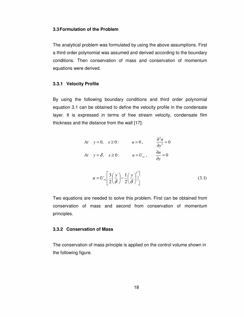
3.3.1 Velocity Profile
By using the following boundary conditions and third order polynomial
equation 3.1 can be obtained to define the velocity profile in the condensate
layer. It is expressed in terms of free stream velocity, condensate film
thickness and the distance from the wall [17]:
Two equations are needed to solve this problem. First can be obtained from
conservation of mass and second from conservation of momentum
principles.
3.3.2 Conservation of Mass
The conservation of mass principle is applied on the control volume shown in
the following figure.
0,:0,
0,0:0,02
2
=∂
∂=≥=
=∂
∂=≥=
∞y
uUuxyAt
y
uuxyAt
δ
)1.3(2
1
2
33
−
= ∞
δδ
yyUu

19
Figure 3.2 Differential Element and Energy Balance on the Liquid Film
Figure 3.3 Flow Area and Heat Transfer Area on Differential Element.
20
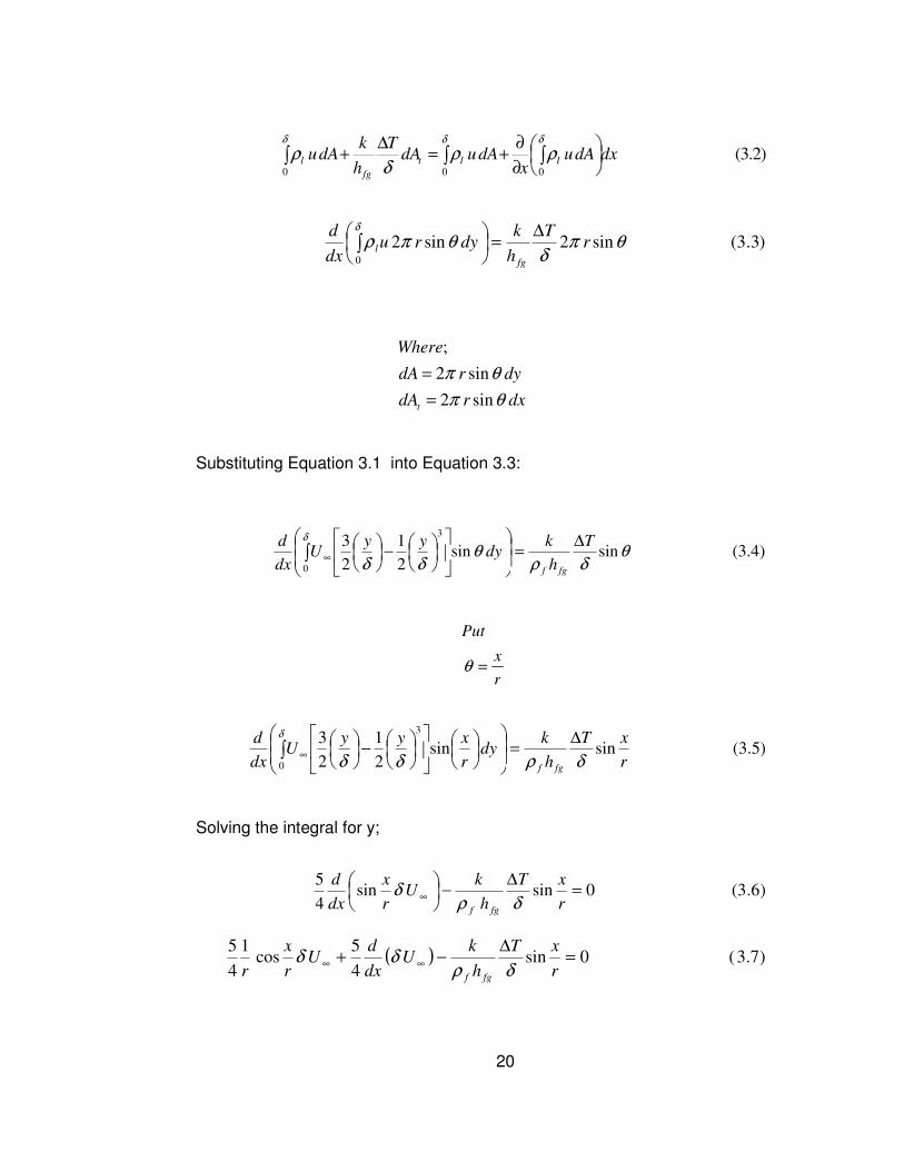
r
x
Put
=θ
Substituting Equation 3.1 into Equation 3.3:
Solving the integral for y;
)3.3(sin2sin20
θπδ
θπρδ
rT
h
kdyru
dx
d
fg
l
∆=
∫
dxrdA
dyrdA
Where
t θπ
θπ
sin2
sin2
;
=
=
)2.3(000
dxdAux
dAudAT
h
kdAu llt
fg
l
∂
∂+=
∆+ ∫∫∫
δδδ
ρρδ
ρ
)5.3(sinsin2
1
2
3
0
3
r
xT
h
kdy
r
xyyU
dx
d
fgf δρδδ
δ ∆=
−
∫ ∞
)6.3(0sinsin4
5=
∆−
∞
r
xT
h
kU
r
x
dx
d
fgf δρδ
( ) )7.3(0sin4
5cos
1
4
5=
∆−+ ∞∞
r
xT
h
kU
dx
dU
r
x
r fgf δρδδ
)4.3(sinsin2
1
2
3
0
3
θδρ
θδδ
δ T
h
kdy
yyU
dx
d
fgf
∆=
−
∫ ∞

21
3.3.3 Conservation of Momentum
The second equation can be obtained from the conservation of momentum
principle. After applying this principle;
fx is body force related with gravity. For the condensate around a sphere;
The shear stress in Equation 3.8 can be expressed with Newton’s law of
viscosity:
Substituting u from Equation 3.1 and taking the derivative, one can obtain:
Recalling Equation 3.1 and integrating Equation 3.8 for y;
( )
)13.3(02
3
)(sin235
34cos
35
34 222
=+
+−+
∞
∞
δµ
δπρδρππρ
U
gr
xrU
dx
dr
r
xfff
)8.3(0sin20
0
2 =+−
=∫ ysxff fdy
r
xru
dx
dτδρπρ
δ
)9.3(sin2 22 grf x θπ=
)10.3(0=
=y
sdy
duµτ
)11.3(2
3
δµτ ∞=
Us
)12.3(02
3)(sin2sin
35
34 222=+−
∞∞
δµδπρδρπ
Ug
r
xrU
r
x
dx
dr ff

22
3.3.4 Heat Transfer Equation
Since only conduction type heat transfer mechanism is assumed at the
beginning of the analysis, heat transfer at the wall in the area dA is;
3.4 Calculation of the Initial Values
We should make some assumptions to begin the calculation from the upper
stagnation point. At the stagnation point the flow velocity is small, so we can
assume that the inertia terms and the pressure gradient in the momentum
equation can be neglected. The momentum equation in the condensate layer
is that:
After eliminating the inertia terms and pressure gradient the momentum
equation comes this form:
After taking the derivative of u twice we can obtain the following equation;
(3.15) sin)(yx
P-
y
)()(f θρµ
ρρg
y
uvu
x
uuf
ff+
∂
∂
∂
∂+
∂
∂=
∂
∂+
∂
∂
3.16)sin2
2
( θρµ ff gy
u−=
∂
∂
)17.3(cycy2
sing21
2f ++−=f
uµ
θρ
( ))14.3(
δwsat TT
kq−
=

23
The boundary conditions are like that:
After applying the boundary conditions Equation 3.17 can be written as :
Initial velocity distribution along the liquid-vapor interface can be obtained
substituting δ into Equation 3.18.
From an energy balance in the condensate layer [16];
The left hand side of this equation is the latent heat of condensation. The
right hand side is the heat transferred from the condensate to the wall over a
length from x=0 to x=x. Equation 3.20 can be rewritten as;
)20.3(220 00
∫∫=
∂
∂=
x
y
fffg dxry
Tkdyruh ππρ
δ
( ) (3.21) x
0 0
∫=
∂
∂=
∂
∂δ
ρyffg
f
y
Tr
h
kdyru
0
00
=→=
=→=
dy
duy
uy
δ
)18.3(2
1sin 22
−=
δδµ
θδρ yygu
f
f
)19.3(2
sin2
f
fgu
µ
θδρ=

24
After substituting the velocity equation in the energy balance, one can obtain
the following equation which gives the condensate layer thickness.
3.5 Finite Difference Equations
Equation 3.7 and Equation 3.13 must be transformed into the finite
differences to solve them numerically. After transforming Equation 3.7 yields;
and Equation 3.13 yields:
Taylor Series expension method can be used to solve these equations.
...)()()()( '
11 +−+= ++ iiiii xfxxxfxf (3.25)
As matrix C corresponds to f(xi), matrix Ψ corresponds to derivative of the
function at xi. xi represents δi and U∞i variables. These are increased with
δinc and Uinc increments, subtracted from their original states and divided by
( )(3.22)
h
31/4
fg
f
−=
g
TTrk
f
wsatf
ρ
υδ
( ))23.3(0sin
4
5cos
4
5 11 =∆
−∆
−+ −∞−∞
∞r
xT
h
k
x
UUU
r
x
r ifgf
iiii
iiδρ
δδδ
( ) ( )
)24.3(02
3)(sin2
35
34cos
35
34
22
2
11
2
2
=+−
−
∆
−+
∞
−∞−∞∞
i
ifi
iiii
fiif
Ug
r
xr
x
UUrU
r
x
δµρδπ
δδρπδπρ

25
corresponding increment. Ψ matrix is two by two square matrix and it is
constituted as:
( )( ) ( )
( )( )
( ) ( )
)28.3(2
3)(sin2
35
34)(cos
35
34
2
3)(sin2
35
34
))((cos35
34
22
2
11
2
2
22
2
11
2
2
)0,1(
inc
i
ifi
iiii
fiif
inci
ifinci
iiiinci
f
iincif
U
r
xgr
x
UUrU
r
x
U
r
xgr
x
UUr
Ur
x
δ
δµρδπ
δδρπδπρ
δδµρδδπ
δδδρπ
δδπρ
ψ
+−
∆
−+
−
+++−
−∆
−+
++
=
∞
−∞−∞∞
∞
−∞−∞
∞
L
( )
( )
)26.3(
sin4
5cos
4
5
sin
4
5)(cos
4
5
11
11
)0,0(
inc
ifgf
fiiii
ii
incifgf
f
iiiinci
iinci
r
x
h
Tk
x
UUU
r
x
r
r
x
h
Tk
x
UUU
r
x
r
δ
δρ
δδδ
δδρ
δδδδδ
ψ
∆−
∆
−+−
+
∆
−∆
−+++
=
−∞−∞∞
−∞−∞∞
L
( )
)27.3(4
5cos
4
5
4
5)(cos
4
5
11
11
)1,0(
inc
iiii
ii
iiincii
incii
U
x
UUU
r
x
r
x
UUUUU
r
x
r
∆
−+−
∆
−+++
=
−∞−∞∞
−∞−∞∞
δδδ
δδδ
ψ

26
To approach to the exact values of velocity and film thickness variables C0,
C1, ψ(0,0), ψ(0,1), ψ(1,0), ψ(1,1) equations have been iterated 20 times. After
finishing the first iteration, by multiplying the inverse of matrix ψ with matrix
C, a vector called as del is found. The velocity and film thickness variables
are updated by adding this vector to the previous iteration. After 20 iterations
the first exact values of velocity (U1) and film thickness (δ1) variables are
found. This cycle is applied to calculate the 18 values of velocity and film
thickness variables.
3.6 Calculation for the Lower Spheres
The condensing falling from the upper sphere creates a film thickness at the
upper stagnation point of the lower sphere. So this film thickness is called as
∆ and it goes to zero as seen in Figure 3.2. The velocity profile is uniform in
( ) ( )
( ) ( )
)29.3(2
3)(sin2
35
34)(cos
35
34
2
3)(sin2
35
34
)(cos35
34
22
2
11
2
2
22
2
11
2
2
)1,1(
inc
i
ifi
iiii
fiif
i
inci
fi
iiincii
f
inciif
U
U
r
xgr
x
UUrU
r
x
UU
r
xgr
x
UUUr
UUr
x
+−
∆
−+
−
++−
∆
−+
++
=
∞
−∞−∞∞
∞
−∞−∞
∞
δµρδπ
δδρπδπρ
δµρδπ
δδρπ
δπρ
ψ L
)30.3(1
0
1
1,10,1
1,00,0
=
=
−
UC
Cdel
δ
ψψ
ψψ

27
this layer. Also as a result of this falling condensing a velocity value occurs
at the upper stagnation point. After completing the iterations for the first
sphere, the effect of film thickness and velocity values falling from the upper
sphere are taken and updated for the lower sphere by using Bernoulli
equation.
The initial velocity and condensate thickness are calculated from Equations
3.16 and 3.22. After this calculation Equations 3.23, 3.24, 3.25 are used to
calculate velocity and condensate thickness for upper sphere as said above.
After finishing the calculations of upper sphere , δinc and Uinc values are
calculated from Equations 3.16 and 3.22. Then the last values of δ and U
which are δ18 and U18 for upper sphere are taken. The condensate thickness
and velocity values are calculated from the following equations for middle
sphere.
Figure 3.4 Physical Model for the Lower Spheres

28
)32.3(
)31.3(2)(
0
18180
2
180
∞
∞
∞∞
=∆
+=
U
U
hgUU
δ
After calculating the initial values for middle sphere, the ∆ thickness is
calculated from the following equation;
Then the ∆ thickness is added to the conservation of mass and momentum
equations. After arranging Equation 3.23 the following equation is obtained;
And after arranging Equation 3.24 the following equation is obtained;
( )
)34.3(0
sin8
5cos
8
5
11
11
=∆
∆−∆
+∆
−∆
−+
−−
−∞−∞∞
x
UU
r
xT
h
k
x
UUU
r
x
r
iiii
ifgf
iiii
iiδρ
δδδ
( ) ( )
)35.3(0)()(
2
3)(sin2
35
34cos
35
34
2
11
222
2
11
2
2
=∆
∆−∆++−
−
∆
−+
−−∞
−∞−∞∞
x
UUUg
r
xr
x
UUrU
r
x
iiii
f
i
i
fi
iiii
fiif
ρδ
µρδπ
δδρπδπρ
)33.3(11
i
iii
U
U
∞
−−∞=∆δ

29
After ∆ goes to zero, Equation 3.23 and Equation 3.24 are used to calculate
velocity and condensate film thickness for the remaining portion of the x axis.
Calculations for the bottom sphere are the same as the middle sphere
calculations.

30
CHAPTER 4
4 EXPERIMENTAL STUDIES
The experimental studies were completly made in ERDEMİR in Machine
Workshop. To do this firstly all parts from screw to the main frame were
designed as 3-D model and then technical drawings were formed. These
drawings were manufactured and assembled in Machine Workshop.
Here three experiments were done. The aim of the first is to measure the
heat transfer rates and heat transfer coefficients for Ø50mm and Ø60mm o.d.
spheres. The aim of the second is to compare the free and forced
condensation results for Ø60mm o.d. sphere and to calculate the local heat
transfer coefficient additionally. The aim of the third study is to obtain datas
for annular condensation in concentric spheres for free and forced
condensations. There are some differences between free condensation
experimental setup and free&forced condensation experimental setup. The
reason behind the differences between the free and free&forced
condensation experimental setups is the experience gained in the free
condensation experiments. After gaining some experience in the free
condensation experiments, improvements were made in the free&forced
condensation experimental setup.
The difference between free and free&forced condensation experimental
setups are the elevation of the cooling water tank, the location of valves, the
source of the water vapour, the location and the numbers of thermocouples.

31
4.1 Case-1 Free Condensation Experimental Study
• The tests were conducted at 0o,12o,20o,30o inclination angles and at
20oC-30oC-40oC-50oC-60oC cooling water inlet temperatures.
• The tests were conducted at Ø50 and Ø60mm o.d.spheres.
• The spheres employed had Ø50mm o.d. Ø44mm i.d.and Ø60mm o.d.
Ø54mm i.d. Inner spheres which had 30mm o.d. were placed in
Ø60mm o.d. spheres and Ø24mm o.d. were placed in Ø50mm o.d.
spheres. The connection of steel water pipe and sphere was achieved
by tight fit.
• The elevation of the cooling water tank from test section was 2 meters.
• Valves were used to prevent the flow of the cooling water so that the
cooling water tank can be filled at the exit of the cooling water
distributing apparatus and three adjustment pieces which were
equipped with adjustment screws were used at the end of the cooling
water exit pipes to adjust the coolant mass flow rate.
• The water vapour was supplied from the steam line of the workshop.
• 11 thermocouples were used. Each sphere was equipped with 2
thermocouples.
4.2 Case-2 Free and Forced Condensation Experimental Study
• The tests were conducted at 0o,5o,10o,15o,20o inclination angles and
at 20oC-30oC-40oC-50oC-60oC cooling water inlet temperatures.
• The tests were conducted for free and forced (only 0o inclination
angle) condensations.
• The spheres employed had 60mm o.d. and 40mm i.d. No internal
spheres were used. The connection between steel water pipe and
sphere was achieved by threads.
• The elevation of the cooling water tank from test section was taken as
3m.

32
• Six valves were used. Three of them were placed at the exit of cooling
water distributing apparatus and the other three were placed at the
end of the cooling water exit pipes.
• A boiler tank was used to supply water vapour to the test section for
free condensation. The steamline of workshop was used for forced
condensation.
• 20 thermocouples were used for free condensation. On each sphere
surface 3 thermocouple and inside of each sphere 2 thermocouples
were placed. 13 thermocouples were used for forced condensation.
4.3 Case-3 Annular Condensation in Concentric Spheres
• The tests were conducted at 0o inclination angle and at 20oC-30oC-
40oC-50oC cooling water inlet temperatures.
• The tests were conducted for free and forced condensations.
• A cylindrical shaped polyamid piece whose inner surface is sphere
was used to make the vapour flow area smaller so that the vapour
flows faster.
• The free and forced condensation experimental setup was used.
• The streamline of workshop was used for forced condensation.
4.4 Experimental Setup
The main parts of the experimental setup are the following :
• Test section
• Cooling Water Tank
• Boiler Tank
• Temperature Reading System
• Main Frame
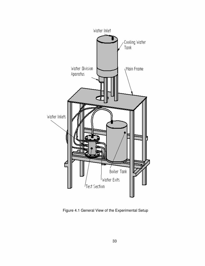
33
Figure 4.1 General View of the Experimental Setup

34
Figure 4.2 General View of the Free Condensation Experimental Setup
Figure 4.3 General View of the Free and Forced Condensation Experimental Setup
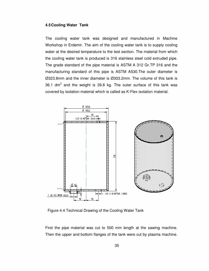
35
4.5 Cooling Water Tank
The cooling water tank was designed and manufactured in Machine
Workshop in Erdemir. The aim of the cooling water tank is to supply cooling
water at the desired temperature to the test section. The material from which
the cooling water tank is produced is 316 stainless steel cold extruded pipe.
The grade standard of the pipe material is ASTM A 312 Gr.TP 316 and the
manufacturing standard of this pipe is ASTM A530.The outer diameter is
Ø323.8mm and the inner diameter is Ø303.2mm. The volume of this tank is
36.1 dm3 and the weight is 39.8 kg. The outer surface of this tank was
covered by isolation material which is called as K-Flex isolation material.
First the pipe material was cut to 500 mm length at the sawing machine.
Then the upper and bottom flanges of the tank were cut by plasma machine.
Figure 4.4 Technical Drawing of the Cooling Water Tank
36
After flanges were welded to the top and bottom of the tank the holes were
drilled at the radial drilling machine. The holes are used for assembling of
cooling water distributing apparatus at the bottom .
At the free condensation experimental setup the water tank was placed 2m
high from the test section. The aim here is to obtain water pressure fixed by
gravity so that the mass flow rate to be the same during the experiments. The
cooling water tank was used only to store water inside it. And no heater was
placed inside it. Water at the desired temperature was obtained from another
tank with a heater on it, which was placed above the cooling water tank. The
cooling water which was caped in 20 dm3 barrels was charged to the heater
tank. The temperature of the cooling water was adjusted by means of the
adjustment button of thermostat. When the temperature of cooling water
reached to the desired value the valve at the exit of the cooling water heating
tank was opened to allow water flow to the cooling water tank. After cooling
water tank was full valves at the exit of the water distributing apparatus were
opened to flow water to the test section.
At the second experimental setup the heigth of the cooling water tank was
increased to 350cm from test section. Here a heater was placed inside the
water tank and a thermometer was placed on the tank. Cooling water was
heated up to desired value inside this tank and supplied to the test section.
4.6 Boiler Tank
Boiler Tank was manufactured from the same pipe used for cooling water
tank. So the dimensions are all same as in the cooling water tank. Boiler tank
has 36.1 dm3 volume and 39.8 kg weight. The manufacturing sequence are
same as the cooling water tank. All drilling operations was made by radial
drilling machine.

37
At the free condensation experimental study the boiler tank was not used.
Instead of that the vapour was obtained from the machine shop. At the free
and forced condensation experimental study an electric heater was
assembled at the bottom of the boiler tank with a heating capacity of 2000W.
4.7 Test Section
The test section was manufactured in Erdemir at machine shop. The material
used is ASTM 316 stainless steel. The test section has three parts.
• Test section body
• Upper cap
• Lower cap
Figure 4.5 Technical Drawing of the Boiler Tank

38
4.7.1 Test Section Body
Manufacturing of the apparatus was started with the manufacturing of the test
section which has three parts. These are test tube, upper flange and lower
flange. Test tube was made from 316 stainless steel material. This material
was cut by sawing machine first. Then inside diameter was machined at the
lathe by leaving 2mm allowance to machine after welding operation because
after flanges are welded to the test tube thermal distorsions which affects the
dimensions occur. This method is used to obtain desired geometrical
tolerances between flanges and test tube, i.e. perpendicularity, parallelism,
concentricity. The upper and lower flanges were manufactured from 316
stainless steel. At the lathe machine circular faces of flanges were machined
and 8 holes were left to be drilled after welding process. After welding
operation of the upper and lower flanges with test tube, the diameter of test
tube and faces of flanges were finished by lathe machine to obtain desired
dimensional and geometrical tolerances. Then the assemble holes over the
flanges were drilled at the coordinate milling machine, which has a digital
coordinate screen. After that the side holes over the test tube were drilled at
the same machine by leaving some allowance to machine after welding
operation of outer rings in which the stainless steel pipe of cooling water is
placed. These outer rings were machined by a lathe machine by leaving
some allowance in their inside diameters. After finishing of them they were
welded on the side holes over the test tube. Then again the test section body
was settled on the coordinate milling machine and the coarse holes of outer
rings and of test tube were drilled together mutually to obtain perfect
eccentricity between the opposite holes and parallelism between the upper
and lower holes. After this operations the dimensional checks were made
and it was seen that the eccentricity and parallelism tolerances were in the
range of 0.01mm to 0.03mm. This eliminates the alignment problem of
spheres.

39
Figure 4.7 Technical Drawing of the Test Section as Isometric View
Figure 4.6 Technical Drawing of the Test Section

40
Figure 4.8 View of the Test Section After Manufacturing Processes
Figure 4.9 View of the Test Section During the Test.

41
4.7.2 Upper And Lower Caps
Finishing the test section body the upper and lower flanges were made. They
also made from 316 stainless steel material. After machining them on the
CNC lathe machine the mounting holes were drilled again on the coordinate
milling machine. For collecting the condensates a hole drilled at the center of
the lower flange. Also the inside surface of the lower flange was machined as
a concave geometry of radius R900mm. A hole was drilled at the center of
the upper flange in order to flow the water vapor to the test section.
Figure 4.10 Technical Drawing of the Lower Cap
Figure 4.11 Technical Drawing of the Upper Cap

42
4.8 Spheres
Spheres were also made in Machine Workshop in Erdemir. The material
used is 316 Stainless Steel. Two different kind of spheres were used in
experiments.
4.8.1 First type of sphere:
Spheres on which condensation is taking place used in the first experiment
had Ø60mm and Ø50mm outer diameter. Because of the spherical shape
and small wall thickness the machining of these spheres are quite difficult.
These spheres were manufactured by machining two hemispheres and
bonding them to each other. The bond material was Loctite Fixmaster
Superior Material. Also Ø34mm diameter spheres made of teflon material the
purpose of which is to accelerate and force the coolant to flow parallel to the
inner surface of the spheres on which condensation is taking place were
Figure 4.12 View of the Upper (left) and Lower (rigth) Caps.

43
used. Three stainless steel pins were machined to pass from the hole at the
center of the Teflon spheres. Before bonding the hemispheres the Ø34mm
diameter spheres were fixed at the center of the steel spheres by welding
the pin to the inner surface of the sphere. Then the bonding material was
applied to the contact surface of the spheres.
After that these hemispheres were connected and after 12 hours the bonding
operation was completely finished. Then the surfaces of the spheres were
polished by polishing machine about 4 hours per sphere.
Figure 4.13 Technical Drawing of the Shpere used in the Free Condensation Experiments.

44
Figure 4.14 First Type of Spheres After Bonding and Polishing
Figure 4.15 First Type of Hemispheres and Inner Sphere

45
4.8.2 Sphere used in the Free&Forced Condensation Experiments
These spheres were used in the free and forced condensation and annular
condensation in the concentric spheres experiments. These spheres also
were made from 316 stainless steel material and had 60mm o.d. and 40mm
i.d.So the thickness of these spheres is 10mm. There were no internal
spheres on them. Similarly two hemispheres were machined to obtain one
sphere. These hemispheres were joint by silver welding after placing the
inner and outer thermocouples which were fastened on the outer and inner
surface on which condensation is taking place by silver welding. On the
contrary of the first type of sphere, instead of 10mm diameter hole a 3/8”-
NPT screw was made. After silver welding process, the sphere surfaces were
polished by polishing machine about 4 hours per sphere.
Figure 4.16 The Placements of the First Type of Spheres in the Test Section.

46
Figure 4.17 Technical Drawing of the Shpere used in the Free&Forced Condensation Experiments.
Figure 4.18 Shpere used in the Free&Forced Condensation Experiments After Silver Welding and Polishing

47
Figure 4.19 Second Type of Spheres with Thermocouples
Figure 4.20 The Placement of Second Type of Spheres in the Test Section.

48
4.9 Vapour Accelerater for Free&Forced Condensation Experiments
In second experimental study to accelerate the vapour a cylinder was used
to make the flow area, through which vapour flows, smaller. To achieve this
the cylinder was placed between the spheres and the test section.
4.10 Vapour Accelerater for Annular Condensation in Concentric
Spheres
At the third experimental study a polyamid cylinder was used to accelerate
the water vapour flowing around the sphere. The inside of this cylinder is
sphere and its diameter is Ø85mm. Polyamid was choosen because being a
plastic material it is easier to machine and since it has a low thermal
conductivity not much condensation occurs on it.
Figure 4.21 The Placement of Vapour Accelerater for Free&Forced Condensation Experiments.

49
4.11 Stainless Steel Pipe Connectors for thr Spheres
These pipes were made from 316 stainless steel material to eliminate
corrosion. They were machined at the lathe. The center was drilled from one
end to other with 10mm drill. Thight fit and threaded types of pipes were
manufactured.
4.11.1 Tight Fit Type of Pipe
It was used at the free condensation experiment. It has 8mm i.d. and 12mm
o.d. at the tips so that it attaches to the sphere with a tight fit. There was no
external screw on this pipe. The hole diameter of the test section was
machined in 0.10mm tolerance to enter this pipe to the test section tigthly
and centered the sphere perfectly. The connection area of sphere and pipe
was insulated with Loctite silicon material to prevent water leakage from
inside of sphere to the outer surface. Also the surface which was left in the
test section was insulated by teflon material to eliminate the condensation on
this surface.
Figure 4.22 Drawing of the Vapour Accelerater for Case-3.

50
4.11.2 Threaded Type of Pipe
It was used at the free&forced condensation and annular condensation in
concentric spheres experiments. Some modifications were made to the tight
fit type of pipe. After free condensation experiment it was seen that some
water leakage was taking place. In the free&forced condensation
experiments to eliminate the leakage problem instead of tight fit at the tip of
the tube 3/8-NPT thread was made. With this method this tube was
Figure 4.23 Technical Drawing of the Tight Fit Type of Pipe
Figure 4.24 The View of the Tight Fit Type of Pipe.

51
connected to the sphere by means of a thread which eliminates cooling water
leakage.
4.12 Cooling Water Distributer Apparatus
The cooling water distributer apparatus was made to distribute the cooling
water comign from cooling water tank to three spheres on which
condensation is taking place equally.
Figure 4.25 Technical Drawing of the Threaded Type of Pipe.
Figure 4.26 Technical Drawing of the Cooling Water Distributer Apparatus, Bottom View.
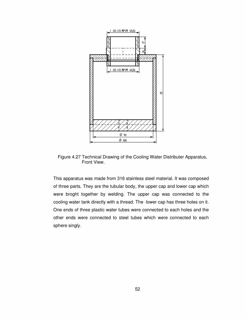
52
This apparatus was made from 316 stainless steel material. It was composed
of three parts. They are the tubular body, the upper cap and lower cap which
were broght together by welding. The upper cap was connected to the
cooling water tank directly with a thread. The lower cap has three holes on it.
One ends of three plastic water tubes were connected to each holes and the
other ends were connected to steel tubes which were connected to each
sphere singly.
Figure 4.27 Technical Drawing of the Cooling Water Distributer Apparatus, Front View.
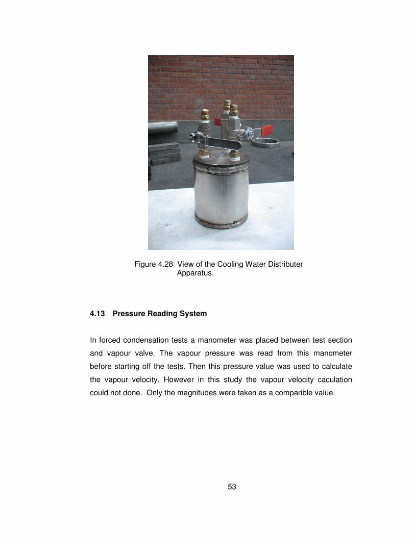
53
4.13 Pressure Reading System
In forced condensation tests a manometer was placed between test section
and vapour valve. The vapour pressure was read from this manometer
before starting off the tests. Then this pressure value was used to calculate
the vapour velocity. However in this study the vapour velocity caculation
could not done. Only the magnitudes were taken as a comparible value.
Figure 4.28 View of the Cooling Water Distributer Apparatus.

54
4.14 Temperature Reading System
In all experiments to read the water inlet&exit temperatures and the surface
temperatures of spheres two thermometers were used. The thermocouples
used are K-Type. On the screen there are 3 digits without any digit after
comma. Because one thermometer has 12 channel for thermocouple
connection, two thermometers were used. These thermometers have +/-1oC
accuracy.
Figure 4.30 View of the Temperature Reading System M3D12x.
Figure 4.29 View of the Pressure Reading System.

55
4.15 Thermocouple Layout
Three different thermocouple placements were used at experiments.
4.15.1 Case-1:Free Condensation Experiment
At the free condensation experiment 11 K-Type thermocouples were used.
On each sphere 2 thermocouples were bonded with Loctite Superior Metal
bonder. One at the upper stagnation point and the other at the midle of the
sphere, 90 degree from upper point. One thermocouple was placed at the
inlet cooling water pipe of the middle sphere. The others were placed at the
cooling water exit pipes for each sphere. The inlet and exit pipes connections
of thermocouples were made by silver welding.
Figure 4.31 The Shematic View of the Thermocouple Layout for Free Condensation Experimental Study.
56
Number 1 : Cooling water inlet of the middle sphere.
Number 2 : Cooling water exit of the upper sphere.
Number 3 : Cooling water exit of the middle sphere.
Number 4 : Cooling water exit of the bottom sphere.
Number 5 : Upper stagnation point of the upper sphere.
Number 6 : Midpoint of outer surface of the upper sphere.
Number 7 : Upper stagnation point of the middle sphere.
Number 8 : Midpoint of outer surface of the middle sphere.
Number 9 : Upper stagnation point of the bottom sphere.
Number 10 : Midpoint of outer surface of the bottom sphere.
Number 11 : Water vapor inlet to the test section.
4.15.2 Case-2:Free&Forced Condensation Experiments
At the free&forced condensation experiments 20 K-Type thermocouples were
used. On each surface of sphere 3 thermocouples were placed by silver
welding method. At the inner surface of spheres 2 thermocouples were
placed one at the upper and the other at the lower points by silver welding.
To do this first thermocouples were welded to the inside surface of spheres
and then two hemispheres were welded to each other by silver electrode.
The placement of the inlet and exit cooling water pipes were not changed.
And the last thermocouple was placed in the test section under the water
vapour inlet nozzle.
Number 1 : Cooling water inlet of the middle sphere.
Number 2 : Cooling water exit of the middle sphere.
Number 3 : Cooling water exit of the upper sphere.
Number 4 : Cooling water exit of the bottom sphere.
Number 5 : Upper stagnation point of the upper sphere.
Number 6 : Midpoint of outer surface of the upper sphere.
Number 7 : Bottom point of the upper sphere
Number 14 : Upper point at the inside of the upper sphere

57
Number 15: Bottom point at the inside of the upper sphere
Number 8 : Upper stagnation point of the middle sphere.
Number 9 : Midpoint of outer surface of the middle sphere..
Number 10: Bottom point of the middle sphere.
Number 16: Upper point at the inside of the middle sphere
Number 17: Bottom point at the inside of the middle sphere
Number 11: Upper stagnation point of the bottom sphere.
Number 12: Midpoint of outer surface of the bottom sphere.
Number 13: Bottom point of the bottom sphere
Number 18: Upper point at the inside of the bottom sphere
Number 19: Bottom point at the inside of the bottom sphere
Number 20: Water vapor inlet to the test section.
Figure 4.32 The Shematic View of the Thermocouple Layout for Free&Forced Condensation Experimental Study.
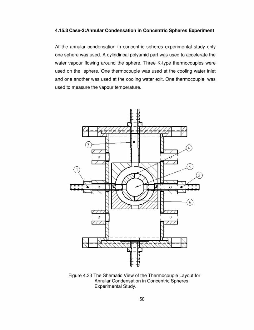
58
4.15.3 Case-3:Annular Condensation in Concentric Spheres Experiment
At the annular condensation in concentric spheres experimental study only
one sphere was used. A cylindirical polyamid part was used to accelerate the
water vapour flowing around the sphere. Three K-type thermocouples were
used on the sphere. One thermocouple was used at the cooling water inlet
and one another was used at the cooling water exit. One thermocouple was
used to measure the vapour temperature.
Figure 4.33 The Shematic View of the Thermocouple Layout for Annular Condensation in Concentric Spheres Experimental Study.
59
Number 1 : Cooling water inlet
Number 2 : Cooling water exit
Number 3 : Vapour inlet
Number 4 : Upper stagnation point
Number 5 : Midpoint of the surface
Number 6 : Lower stagnation point
4.16 Data Collecting Method
The test were done several times by using the same parameters. After
obtaining the values, some results were eliminated. The other results were
added to each other and the arithmetic averages were calculated as a one
value. And these values were used in the heat transfer calculations.
4.17 Thermometer Calibration
Before starting to setup the thermocouples the reader must be checked. To
do this a milivolt generator device is used. First of all this device is connected
to the reader and then electricity is opened. From the milivolt-temperature
graphs milivolt value of the choosen temperature is read. Then this milivolt is
given to the reader via the generator and the temperature value is read from
the reader screen. In this study this check was made before starting test. It
was seen that reader shows temperature values 10oC greather than the real
values.
After connecting thermocouples to the readers again temperatures were read
from readers and from another thermometer. For this purpose temperature of
stationary air was measured by both of them. Also for higher temperature
value water was heated to desired value and measured by both of them. It
was seen that the readings were 4oC higher than the real values.
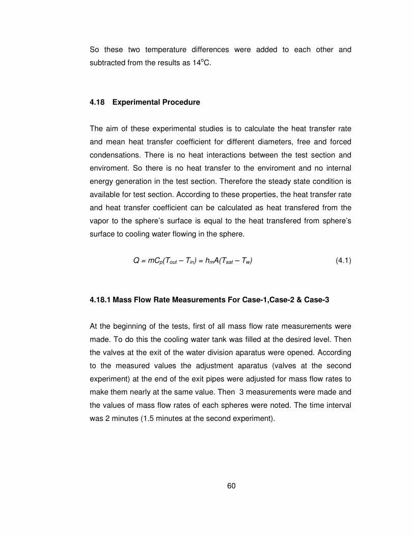
60
So these two temperature differences were added to each other and
subtracted from the results as 14oC.
4.18 Experimental Procedure
The aim of these experimental studies is to calculate the heat transfer rate
and mean heat transfer coefficient for different diameters, free and forced
condensations. There is no heat interactions between the test section and
enviroment. So there is no heat transfer to the enviroment and no internal
energy generation in the test section. Therefore the steady state condition is
available for test section. According to these properties, the heat transfer rate
and heat transfer coefficient can be calculated as heat transfered from the
vapor to the sphere’s surface is equal to the heat transfered from sphere’s
surface to cooling water flowing in the sphere.
Q = mCp(Tout – Tin) = hmA(Tsat – Tw) (4.1)
4.18.1 Mass Flow Rate Measurements For Case-1,Case-2 & Case-3
At the beginning of the tests, first of all mass flow rate measurements were
made. To do this the cooling water tank was filled at the desired level. Then
the valves at the exit of the water division aparatus were opened. According
to the measured values the adjustment aparatus (valves at the second
experiment) at the end of the exit pipes were adjusted for mass flow rates to
make them nearly at the same value. Then 3 measurements were made and
the values of mass flow rates of each spheres were noted. The time interval
was 2 minutes (1.5 minutes at the second experiment).

61
4.18.2 Case-1 Free Condensation Experiments
The tests were conducted at 0o,12o,20o,30o inclination angles and at 20oC-
30oC-40oC-50oC-60oC cooling water inlet temperatures. In the first study the
results of Ø50mm and Ø60mm o.d. spheres were obtained and compared for
free condensation.
Water vapour was supplied from steam line. The vapour valve is opened. At
the same time the air exit valve is opened. Test section is waited about 60
minutes to be completly filled by water vapour. After 60 minutes the air exit
valve is closed. The aim of this procedure is to eliminate the air inside the
test section to obtain complete condensation. Then the cooling water is
heated up to the desired temperature in the tank. When the temperature is
reached to the desired point the valves are opened and cooling water runs
inside the spheres. About 2 minutes are waited to obtain steady state
condition by wacthing the thermocouple reader. When the temperatures are
not changed the values are read and noted. The cooling water is collected at
the vessels which are placed under each water exit pipes of spheres. The
condensation is also collected in another vessel. After readings the valves
are closed. The vessels are weighed at the digital heaviness and noted.
4.18.3 Case:2 Free&Forced Condensation Experiments
The tests were conducted at 0o,5o,10o,15o,20o inclination angles and at 25oC-
30oC-40oC-50oC cooling water inlet temperatures. In the second study datas
are obtained for free and forced condensations.
Water vapour is supplied from boiler which has a 2.5kW heater for free
condensation. The heater is plugged. About 60 minutes later the water
vapour srarts to occur. At the same time the air exit valve is opened. Test
section is waited about 60 minutes to be completly filled by water vapour.
After 60 minutes the air exit valve is closed. The aim of this procedure is to

62
eliminate the air inside the test section to obtain complete condensation.
Then the cooling water is heated up to the desired temperature in the tank.
When the temperature is reached to the desired point the valves are opened
and cooling water runs inside the spheres. About 2 minutes are waited to
obtain steady state condition by wacthing the thermocouple reader. When the
temperatures are not changed the values are read and noted. The cooling
water is collected at the vessels which are placed under each water exit
pipes of spheres. The condensation is also collected in another vessel. After
readings the valves are closed. The vessels are weighed at the digital
heaviness and noted. From 20 termocouples 20 temperature values are
read. For forced condensation a manometer is used to read the vapour
pressure which is coming from the steamline of workshop.
4.18.4 Case:3 Annular Condensation in the Concentric Spheres
The tests were conducted at 0o inclination angles and at 20oC-30oC-40oC-
50oC cooling water inlet temperatures. In this study datas are obtained for
forced and free condensations.
The aim of third experimental study is to obtain the data for water vapour
flowing between to sphere surfaces. To do this a cylindirical part is used.
Inside of this part is spherical shaped and has Ø85mm diameter. The steel
sphere is placed inside this part. There is 12.5mm space between the
surfaces and water vapour flows in this space. Datas are obtained for this
situation. At least two measurements are made to obtain the reliable results
and then the average of them is taken. For forced condensation steamline is
used to obtain high velocity vapour.
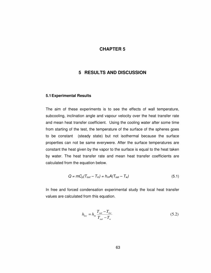
63
CHAPTER 5
5 RESULTS AND DISCUSSION
5.1 Experimental Results
The aim of these experiments is to see the effects of wall temperature,
subcooling, inclination angle and vapour velocity over the heat transfer rate
and mean heat transfer coefficient. Using the cooling water after some time
from starting of the test, the temperature of the surface of the spheres goes
to be constant (steady state) but not isothermal because the surface
properties can not be same everywere. After the surface temperatures are
constant the heat given by the vapor to the surface is equal to the heat taken
by water. The heat transfer rate and mean heat transfer coefficients are
calculated from the equation below.
Q = mCp(Tout – Tin) = hmA(Tsat – Tw) (5.1)
In free and forced condensation experimental study the local heat transfer
values are calculated from this equation.
)2.5(wsat
locsatmloc
TT
TThh
−
−=

64
5.1.1 Case 1- Free Condensation Experiments
The tests were conducted at 0o,12o,20o,30o inclination angles and at 20oC-
30oC-40oC-50oC-60oC cooling water inlet temperatures. Datas were obtained
for Ø50mm and Ø60mm o.d. spheres. In all experiments the effect of mass
flow rate of cooling water is considered.
To eliminate the cooling water pressure drop the water tank was placed
200cm above the test section. The mass flow rates were adjusted by using
valves. Only the Ø60mm o.d. sphere results are given in the following
figures. The Ø50mm o.d. sphere results are given in Appendix-C.
The calculated equations for mass flow rates are as follows.
m1(t)=-0,00458.(t-t1)+m1 (5.3)
m2(t)=-0,00139.(t-t2)+m2 (5.4)
m3(t)=-0,00222.(t-t3)+m3 (5.5)
Mass Flow Rate Variations
5
7
9
11
13
15
150 300 600
Time (s)
Mas
s F
low
Rat
e (g
/s)
Upper Middle Bottom
Figure 5.1 Experimental Mass Flow Rate Variation with respect to Time
for Case-1, D=Ø60mm.
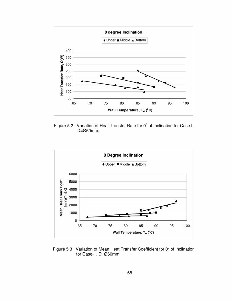
65
0 degree Inclination
50
100
150
200
250
300
350
400
65 70 75 80 85 90 95 100
Wall Temperature, Tw (oC)
Hea
t T
ran
sfer
Rat
e, Q
(W)
Upper Middle Bottom
0 Degree Inclination
0
1000
2000
3000
4000
5000
6000
65 70 75 80 85 90 95 100
Wall Temperature, Tw (oC)
Mea
n H
eat
Tra
ns.
Co
eff.
h
m(W
/m2K
)
Upper Middle Bottom
Figure 5.2 Variation of Heat Transfer Rate for 0o of Inclination for Case1, D=Ø60mm.
Figure 5.3 Variation of Mean Heat Transfer Coefficient for 0o of Inclination for Case-1, D=Ø60mm.

66
12 Degree Inclination
50
100
150
200
250
300
350
400
65 70 75 80 85 90 95 100
Wall Temperature,Tw (oC)
Hea
t T
ran
sfer
Rat
e, Q
(W)
Upper Middle Bottom
12 Degree Inclination
0
1000
2000
3000
4000
5000
6000
65 70 75 80 85 90 95 100
Wall Temperature,Tw (oC)
Mea
n H
eat
Tra
ns.
Co
eff.
h
m(W
/m2K
)
Upper Middle Bottom
Figure 5.4 Variation of Heat Transfer Rate for 12o of Inclination for Case-1, D=Ø60mm.
Figure 5.5 Variation of Mean Heat Transfer Coefficient for 12o of Inclination for Case-1, D=Ø60mm.

67
20 Degree Inclination
50
100
150
200
250
300
350
400
65 70 75 80 85 90 95 100
Wall Temperature, Tw (oC)
Hea
t T
ran
sfer
Rat
e, Q
(W)
Upper Middle Bottom
20 Degree Inclination
0
1000
2000
3000
4000
5000
6000
65 70 75 80 85 90 95 100
Wall Temperature, Tw (oC)
Mea
n H
eat
Tra
ns.
Co
eff.
h
m(W
/m2K
)
Upper Middle Bottom
Figure 5.6 Variation of Heat Transfer Rate for 20o of Inclination for Case-1, D=Ø60mm.
Figure 5.7 Variation of Mean Heat Transfer Coefficient for 20o of Inclination
for Case-1, D=Ø60mm.
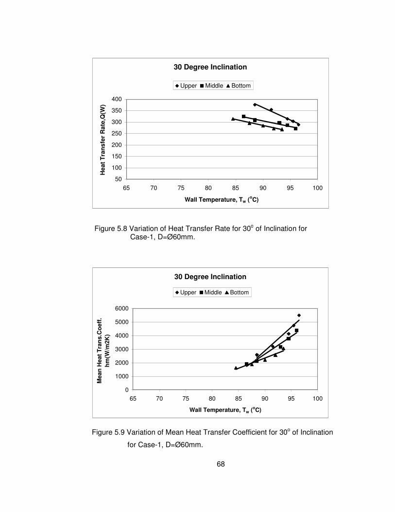
68
30 Degree Inclination
50
100
150
200
250
300
350
400
65 70 75 80 85 90 95 100
Wall Temperature, Tw (oC)
Hea
t T
ran
sfer
Rat
e,Q
(W)
Upper Middle Bottom
30 Degree Inclination
0
1000
2000
3000
4000
5000
6000
65 70 75 80 85 90 95 100
Wall Temperature, Tw (oC)
Mea
n H
eat
Tra
ns.
Co
eff.
h
m(W
/m2K
)
Upper Middle Bottom
Figure 5.8 Variation of Heat Transfer Rate for 30o of Inclination for Case-1, D=Ø60mm.
Figure 5.9 Variation of Mean Heat Transfer Coefficient for 30o of Inclination
for Case-1, D=Ø60mm.

69
5.1.2 Comparison of the Results of Ø50mm and Ø60mm Spheres
Heat flux and mean heat transfer coefficient results were obtained for
Ø50mm and Ø60mm o.d. spheres. They are compared at the following
figures for 0o and 12o inclination angles.
It is seen from these figures that when the diameter gets bigger the heat flux
and heat transfer coefficients get smaller because the film thickness gets
thicker. And this tchicker film tchikness makes a barrier to resist heat
transfer.
Upper Sphere
0
5000
10000
15000
20000
25000
30000
35000
40000
80 85 90 95 100
Wall Temperature,Tw
Hea
t F
lux,
q
Ø60 Sphere Ø50 Sphere
Figure 5.10 Comparison of Heat Flux for 0o Inclination Angle for Upper Sphere, D=Ø50mm and D=Ø60mm.

70
Middle Sphere
0
5000
10000
15000
20000
25000
30000
35000
40000
65 70 75 80 85 90 95
Wall Temperature,Tw
Hea
t F
lux,
q
Ø60 Sphere Ø50 Sphere
Bottom Sphere
0
5000
10000
15000
20000
25000
30000
35000
40000
65 70 75 80 85 90 95
Wall Temperature,Tw
Hea
t F
lux,
q
Ø60 Sphere Ø50 Sphere
Figure 5.11 Comparison of Heat Flux for 0o Inclination Angle for Middle Sphere, D=Ø50mm and D=Ø60mm. .
Figure 5.12 Comparison of Heat Flux for 0o Inclination Angle for Bottom Sphere, D=Ø50mm and D=Ø60mm.

71
Upper Sphere
0
500
1000
1500
2000
2500
3000
3500
84 86 88 90 92 94 96 98
Wall Temperature,Tw
Hea
t T
ran
sfer
Co
eff.
,h
Ø60 Sphere Ø50 Sphere
Middle Sphere
0
200
400
600
800
1000
1200
1400
70 75 80 85 90 95
Wall Temperature,Tw
Hea
t T
ran
sfer
Co
eff.
,h
Ø60 Sphere Ø50 Sphere
Figure 5.13 Comparison of Mean Heat Transfer Coefficient for 0oInclination Angle for Upper Sphere, D=Ø50mm and D=Ø60mm.
Figure 5.14 Comparison of Mean Heat Transfer Coefficient for 0oInclination Angle for Middle Sphere, D=Ø50mm and D=Ø60mm.

72
Bottom Sphere
0
100
200
300
400
500
600
700
800
900
65 70 75 80 85 90 95
Wall Temperature,Tw
Hea
t T
ran
sfer
Co
eff.
,h
Ø60 Sphere Ø50 Sphere
Upper Sphere,12o Inclination
0
500
1000
1500
2000
2500
3000
3500
4000
82 84 86 88 90 92 94 96 98
Wall Temperature,Tw
Hea
t T
ran
sfer
Co
eff.
,h
Ø60 Sphere Ø50 Sphere
Figure 5.15 Comparison of Mean Heat Transfer Coefficient for 0oInclination Angle for Bottom Sphere, D=Ø50mm and D=Ø60mm.
Figure 5.16 Comparison of Mean Heat Transfer Coefficient for 12o Inclination Angle for Upper Sphere, D=Ø50mm and D=Ø60mm.

73
Middle Sphere,12o Inclination
0
500
1000
1500
2000
2500
70 75 80 85 90 95
Wall Temperature,Tw
Hea
t T
ran
sfer
Co
eff.
,h
Ø60 Sphere Ø50 Sphere
Bottom Sphere,12o Inclination
0
200
400
600
800
1000
1200
1400
1600
65 70 75 80 85 90 95
Wall Temperature,Tw
Hea
t T
ran
sfer
Co
eff.
,h
Ø60 Sphere Ø50 Sphere
Figure 5.17 Comparison of Mean Heat Transfer Coefficient for 12o Inclination Angle for Middle Sphere, D=Ø50mm and D=Ø60mm.
Figure 5.18 Comparison of Mean Heat Transfer Coefficient for 12o Inclination Angle for Bottom Sphere, D=Ø50mm and D=Ø60mm.
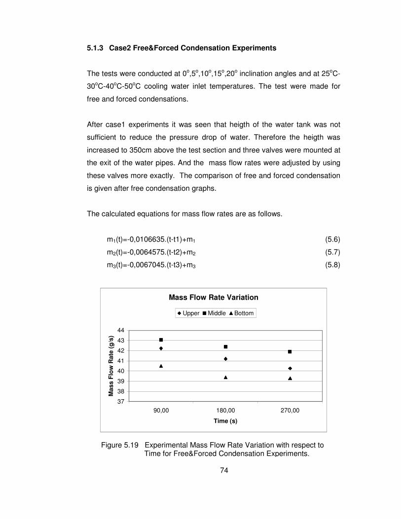
74
5.1.3 Case2 Free&Forced Condensation Experiments
The tests were conducted at 0o,5o,10o,15o,20o inclination angles and at 25oC-
30oC-40oC-50oC cooling water inlet temperatures. The test were made for
free and forced condensations.
After case1 experiments it was seen that heigth of the water tank was not
sufficient to reduce the pressure drop of water. Therefore the heigth was
increased to 350cm above the test section and three valves were mounted at
the exit of the water pipes. And the mass flow rates were adjusted by using
these valves more exactly. The comparison of free and forced condensation
is given after free condensation graphs.
The calculated equations for mass flow rates are as follows.
m1(t)=-0,0106635.(t-t1)+m1 (5.6)
m2(t)=-0,0064575.(t-t2)+m2 (5.7)
m3(t)=-0,0067045.(t-t3)+m3 (5.8)
Mass Flow Rate Variation
37
38
39
40
41
42
43
44
90,00 180,00 270,00
Time (s)
Mas
s F
low
Rat
e (g
/s)
Upper Middle Bottom
Figure 5.19 Experimental Mass Flow Rate Variation with respect to Time for Free&Forced Condensation Experiments.
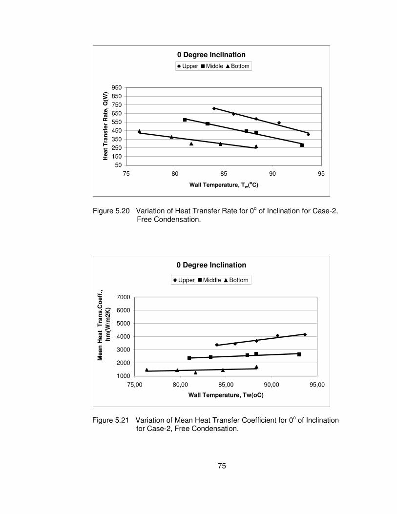
75
0 Degree Inclination
50150
250350
450550
650750
850950
75 80 85 90 95
Wall Temperature, Tw(oC)
Hea
t T
ran
sfer
Rat
e, Q
(W)
Upper Middle Bottom
0 Degree Inclination
1000
2000
3000
4000
5000
6000
7000
75,00 80,00 85,00 90,00 95,00
Wall Temperature, Tw(oC)
Mea
n H
eat
Tra
ns.
Co
eff.
, h
m(W
/m2K
)
Upper Middle Bottom
Figure 5.20 Variation of Heat Transfer Rate for 0o of Inclination for Case-2, Free Condensation.
Figure 5.21 Variation of Mean Heat Transfer Coefficient for 0o of Inclination for Case-2, Free Condensation.

76
5 Degree Inclination
50
150
250
350
450
550
650
750
850
950
70 75 80 85 90 95
Wall Temperature, Tw(oC)
Hea
t T
ran
sfer
Rat
e, Q
(W)
Upper Middle Bottom
5 Degree Inclination
1000
2000
3000
4000
5000
6000
7000
70 75 80 85 90 95
Wall Temperature, Tw(oC)
Mea
n H
eat
Tra
ns.
Co
eff.
h
m(W
/m2K
)
Upper Middle Bottom
Figure 5.22 Variation of Heat Transfer Rate for 5o of Inclination for Case-2, Free Condensation.
Figure 5.23 Variation of Mean Heat Transfer Coefficient for 5o of Inclination for Case-2, Free Condensation.

77
10 Degree Inclination
50150
250
350
450
550
650
750
850
950
70 75 80 85 90 95
Wall Temperature, Tw(oC)
Hea
t T
ran
sfer
Rat
e, Q
(W)
Upper Middle Bottom
10 Degree Inclination
1000
2000
3000
4000
5000
6000
7000
70 75 80 85 90 95
Wall Temperature, Tw(oC)
Mea
n H
eat
Tra
ns.
Co
eff.
h
m(W
/m2K
)
Upper Middle Bottom
Figure 5.24 Variation of Heat Transfer Rate for 10o of Inclination for Case-2, Free Condensation.
Figure 5.25 Variation of Mean Heat Transfer Coefficient for 10o of Inclination for Case-2, Free Condensation.

78
15 Degree Inclination
50150250350450550650750850950
70 75 80 85 90 95
Wall Temperature, Tw(oC)
Hea
t T
ran
sfer
Rat
e, Q
(W)
Upper Middle Bottom
15 Degree Inclination
1000
2000
3000
4000
5000
6000
7000
70 75 80 85 90 95
Wall Temperature, Tw(oC)
Mea
n H
eat
Tra
ns.
Co
eff.
h
m(W
/m2K
)
Upper Middle Bottom
Figure 5.26 Variation of Heat Transfer Rate for 15o of Inclination for Case-2, Free Condensation.
Figure 5.27 Variation of Mean Heat Transfer Coefficient for 15o of Inclination for Case-2, Free Condensation.

79
20 Degree Inclination
50
150
250
350
450
550
650
750
850
950
70 75 80 85 90 95 100
Wall Temperature, Tw(oC)
Hea
t T
ran
sfer
Rat
e, Q
(W)
Upper Middle Bottom
20 Degree Inclination
1000
2000
3000
4000
5000
6000
7000
70 75 80 85 90 95
Wall Temperature, Tw(oC)
Mea
n H
eat
Tra
ns.
Co
eff.
h
m(W
/m2K
)
Upper Middle Bottom
Figure 5.28 Variation of Heat Transfer Rate for 20o of Inclination for Case-2, Free Condensation.
Figure 5.29 Variation of Mean Heat Transfer Coefficient for 20o of Inclination for Case-2, Free Condensation.
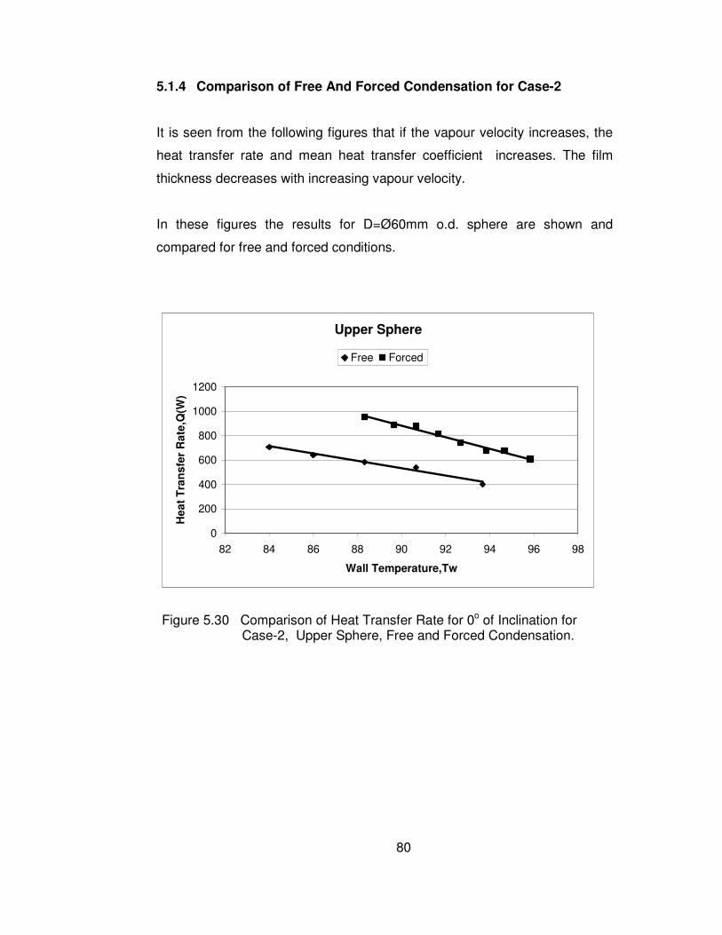
80
5.1.4 Comparison of Free And Forced Condensation for Case-2
It is seen from the following figures that if the vapour velocity increases, the
heat transfer rate and mean heat transfer coefficient increases. The film
thickness decreases with increasing vapour velocity.
In these figures the results for D=Ø60mm o.d. sphere are shown and
compared for free and forced conditions.
Upper Sphere
0
200
400
600
800
1000
1200
82 84 86 88 90 92 94 96 98
Wall Temperature,Tw
Hea
t T
ran
sfer
Rat
e,Q
(W)
Free Forced
Figure 5.30 Comparison of Heat Transfer Rate for 0o of Inclination for Case-2, Upper Sphere, Free and Forced Condensation.

81
Middle Sphere
0100200300400500600700800900
1000
80 82 84 86 88 90 92 94 96
Wall Temperature,Tw
Hea
t T
ran
sfer
Rat
e,Q
(W)
Free Forced
Bottom Sphere
0
100
200
300
400
500
600
700
800
900
70 75 80 85 90 95
Wall Temperature,Tw
Hea
t T
ran
sfer
Rat
e,Q
(W)
Free Forced
Figure 5.31 Comparison of Heat Transfer Rate for 0o of Inclination for Case-2, Middle Sphere, Free and Forced Condensation.
Figure 5.32 Comparison of Heat Transfer Rate for 0o of Inclination for Case-2, Bottom Sphere, Free and Forced Condensation.

82
Middle Sphere
0
1000
2000
3000
4000
5000
6000
7000
80 82 84 86 88 90 92 94 96
Wall Temperature,Tw
Mea
n H
eat
Tra
nsf
er C
oef
f.,h
Free Forced
Upper Sphere
0100020003000400050006000700080009000
82 84 86 88 90 92 94 96 98
Wall Temperature,Tw
Mea
n H
eat
Tra
nsf
er C
oef
f.,h
Free Forced
Figure 5.33 Comparison of Mean Heat Transfer Coefficients for 0o of Inclination for Case-2,Upper Sphere, Free and Forced
Condensation.
Figure 5.34 Comparison of Mean Heat Transfer Coefficients for 0o of Inclination for Case-2,Middle Sphere, Free and Forced Condensation.

83
Bottom Sphere
0
1000
2000
3000
4000
5000
6000
70 75 80 85 90 95
Wall Temperature,Tw
Mea
n H
eat
Tra
nsf
er C
oef
f.,h
Free Forced
5.1.5 Case 3 Annular Condensation in the Concentric Spheres
The tests were conducted at 0o inclination angle and at 20oC-30oC-40oC-
50oC-60oC cooling water inlet temperatures for free and forced
condensations.
The calculated equation for mass flow rate is as follows.
m1(t)=-001829457.(t-t1)+m1 (5.9)
Figure 5.35 Comparison of Mean Heat Transfer Coefficients for 0o of Inclination for Case-2,Bottom Sphere, Free and Forced
Condensation.

84
Mass Flow Rate Variation
20,00
21,00
22,00
23,00
24,00
25,00
26,00
27,00
94 90 150 120 120 165
Time (s)
Mas
s F
low
Rat
e (g
/s)
0 Degree Inclination
0
50
100
150
200
250
300
350
400
450
500
93 93 94 95 97 97 97
Wall Temperature, Tw(oC)
Mea
n H
eat
Tra
nsf
er R
ate,
Q(W
)
Figure 5.36 Experimental Mass Flow Rate Variation with respect to Time for Annular Condensation in Concentric Spheres.
Figure 5.37 Variation of Mean Heat Transfer Rate for 0o of Inclination for Annular Condensation in Concentric Spheres.
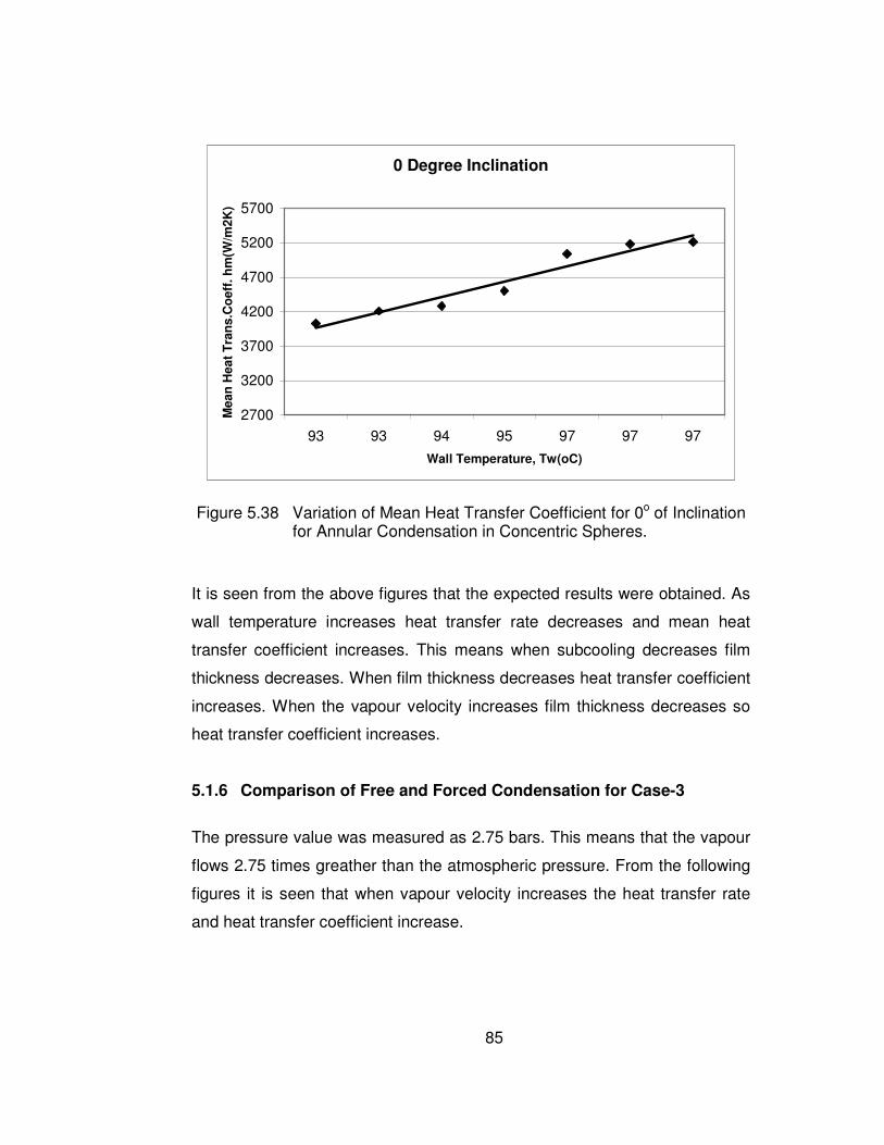
85
It is seen from the above figures that the expected results were obtained. As
wall temperature increases heat transfer rate decreases and mean heat
transfer coefficient increases. This means when subcooling decreases film
thickness decreases. When film thickness decreases heat transfer coefficient
increases. When the vapour velocity increases film thickness decreases so
heat transfer coefficient increases.
5.1.6 Comparison of Free and Forced Condensation for Case-3
The pressure value was measured as 2.75 bars. This means that the vapour
flows 2.75 times greather than the atmospheric pressure. From the following
figures it is seen that when vapour velocity increases the heat transfer rate
and heat transfer coefficient increase.
Figure 5.38 Variation of Mean Heat Transfer Coefficient for 0o of Inclination for Annular Condensation in Concentric Spheres.
0 Degree Inclination
2700
3200
3700
4200
4700
5200
5700
93 93 94 95 97 97 97
Wall Temperature, Tw(oC)
Mea
n H
eat
Tra
ns.
Co
eff.
hm
(W/m
2K)
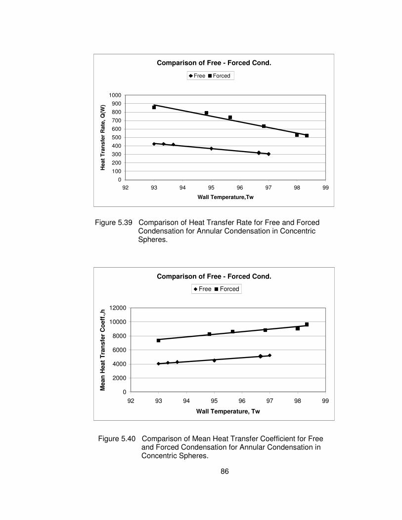
86
Comparison of Free - Forced Cond.
0
2000
4000
6000
8000
10000
12000
92 93 94 95 96 97 98 99
Wall Temperature, Tw
Mea
n H
eat
Tra
nsf
er C
oef
f.,h
Free Forced
Comparison of Free - Forced Cond.
0
100
200
300
400
500
600
700
800
900
1000
92 93 94 95 96 97 98 99
Wall Temperature,Tw
Hea
t T
ran
sfer
Rat
e, Q
(W)
Free Forced
Figure 5.39 Comparison of Heat Transfer Rate for Free and Forced Condensation for Annular Condensation in Concentric Spheres.
Figure 5.40 Comparison of Mean Heat Transfer Coefficient for Free and Forced Condensation for Annular Condensation in Concentric Spheres.

87
5.1.7 Effect of Wall Temperature
It is seen from the above figures that when the wall temperature increases
near to the saturation temperature the heat transfer rate decreases due to
the subcooling. The increase in the wall temperature yields to decrease in
subcooling. Also when the heat transfer rate increases the film thickness also
increases and it results in lower heat transfer coefficients. So when the wall
temperature approaches to the saturation temperature mean heat transfer
coefficient increases. Also from these figures it is seen that the upper sphere
has higher heat transfer rates and heat transfer coefficients then the middle
and bottom spheres. The cause is the condensation flow. The condensation
coming from the upper sphere to the middle sphere and from it to the bottom
sphere results in thicker condensation thickness and it prevents the heat
transfer and the heat transfer rate and mean heat transfer coefficient
decrase.
5.1.8 Effect of Subcooling
It is seen from the above figures that when the subcooling decreases heat
transfer rate decreases but the mean heat transfer coefficient increases. The
reason for decrease of subcooling is the decrease of condensate film
thickness. It means the heat transfer coefficient increases. Also the
subcooling decreases at the bottom spheres because of the cooling effect of
the condensate coming from upper sphere.
5.1.9 Effect of Inclination Angle
It is shown from the above figures that when the inclination angle increases
the heat transfer rate and heat transfer coefficient increase at the middle and
bottom spheres. Because of the inclination angle the cooling effect of the
condesate falling from upper sphere to lower sphere reduces and also
subcooling reduces. So when the degree is 30 the condenaste coming from
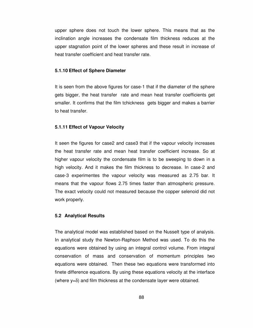
88
upper sphere does not touch the lower sphere. This means that as the
inclination angle increases the condensate film thickness reduces at the
upper stagnation point of the lower spheres and these result in increase of
heat transfer coefficient and heat transfer rate.
5.1.10 Effect of Sphere Diameter
It is seen from the above figures for case-1 that if the diameter of the sphere
gets bigger, the heat transfer rate and mean heat transfer coefficients get
smaller. It confirms that the film tchickness gets bigger and makes a barrier
to heat transfer.
5.1.11 Effect of Vapour Velocity
It seen the figures for case2 and case3 that if the vapour velocity increases
the heat transfer rate and mean heat transfer coefficient increase. So at
higher vapour velocity the condensate film is to be sweeping to down in a
high velocity. And it makes the film thickness to decrease. In case-2 and
case-3 experimentes the vapour velocity was measured as 2.75 bar. It
means that the vapour flows 2.75 times faster than atmospheric pressure.
The exact velocity could not measured because the copper selenoid did not
work properly.
5.2 Analytical Results
The analytical model was established based on the Nusselt type of analysis.
In analytical study the Newton-Raphson Method was used. To do this the
equations were obtained by using an integral control volume. From integral
conservation of mass and conservation of momentum principles two
equations were obtained. Then these two equations were transformed into
finete difference equations. By using these equations velocity at the interface
(where y=δ) and film thickness at the condensate layer were obtained.
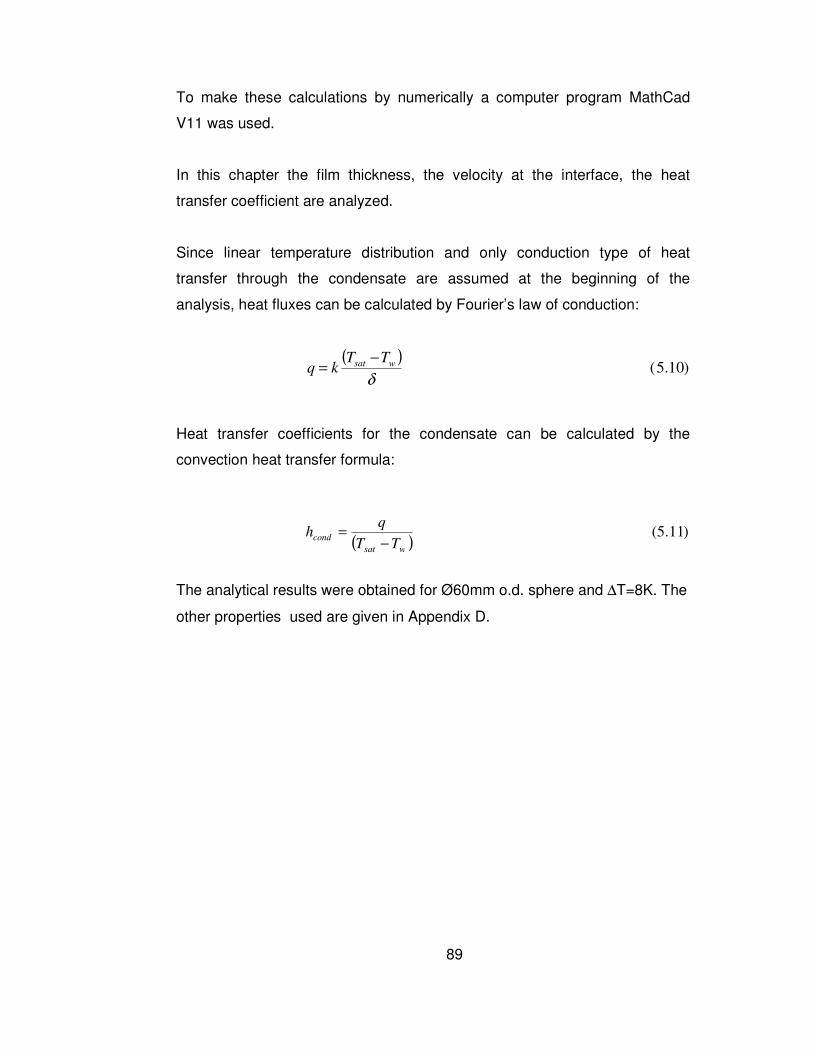
89
To make these calculations by numerically a computer program MathCad
V11 was used.
In this chapter the film thickness, the velocity at the interface, the heat
transfer coefficient are analyzed.
Since linear temperature distribution and only conduction type of heat
transfer through the condensate are assumed at the beginning of the
analysis, heat fluxes can be calculated by Fourier’s law of conduction:
Heat transfer coefficients for the condensate can be calculated by the
convection heat transfer formula:
The analytical results were obtained for Ø60mm o.d. sphere and ∆T=8K. The
other properties used are given in Appendix D.
( ))10.5(
δwsat TT
kq−
=
( ))11.5(
wsat
condTT
qh
−=

90
Film Thickness Variations
0,00014
0,00016
0,00018
0,0002
0,00022
0,00024
0,00026
0,00028
0,0003
8 24 40 56 72 88 104
120
136
Degree, θθθθ
Film
Th
ickn
ess
δ (
δ (
δ (δ (
m)
Upper Sphere Middle Sphere Lower Sphere
Velocity Variations
0,00001
0,000015
0,00002
0,000025
0,00003
0,000035
0,00004
0,000045
0,00005
0,000055
0,00006
8 16 24 32 40 48 56 64 72 80 88 96 104 112 120 128 136 144
Degree, θθθθ
Vel
oci
ty (
m/s
)
Upper Sphere Middle Sphere Lower Sphere
Figure 5.41 Variation of Film Thickness with Angular Position at D=60mm and ∆T=8K
Figure 5.42 Variation of Velocity of the Condensate with Angular Position at D=60mm and ∆T=8K
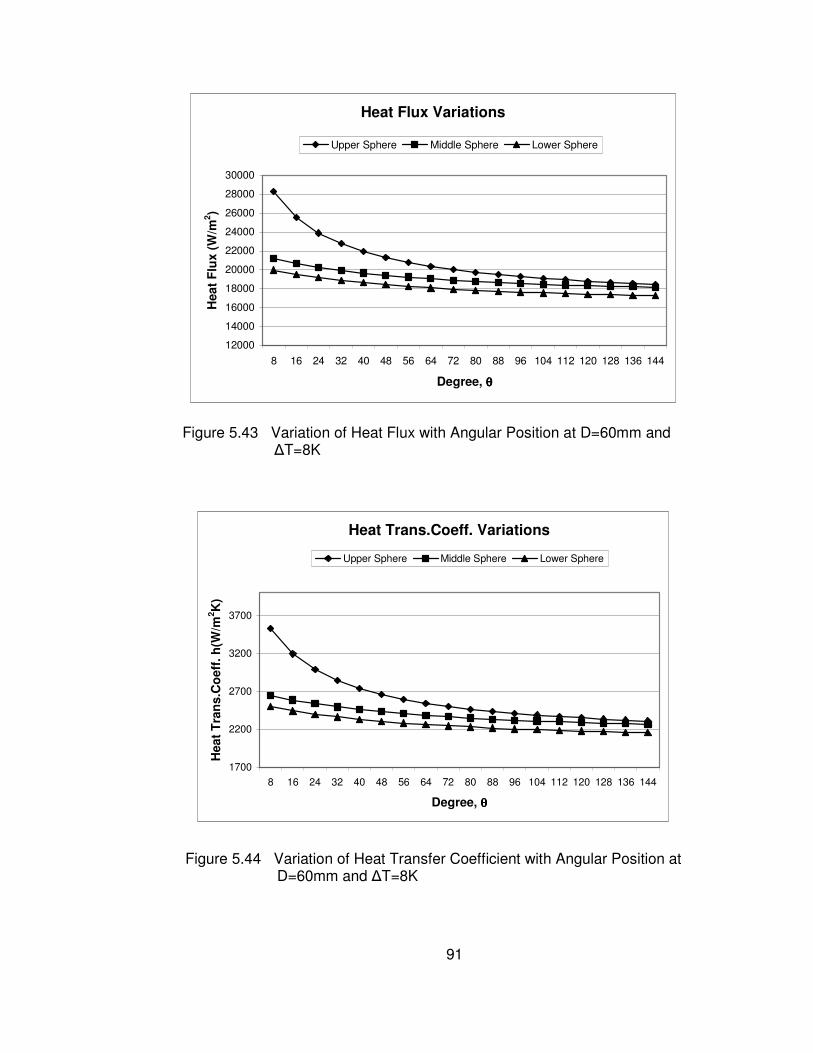
91
Heat Flux Variations
12000
14000
16000
18000
20000
22000
24000
26000
28000
30000
8 16 24 32 40 48 56 64 72 80 88 96 104 112 120 128 136 144
Degree, θθθθ
Hea
t F
lux
(W/m
2 )
Upper Sphere Middle Sphere Lower Sphere
Heat Trans.Coeff. Variations
1700
2200
2700
3200
3700
8 16 24 32 40 48 56 64 72 80 88 96 104 112 120 128 136 144
Degree, θθθθ
Hea
t T
ran
s.C
oef
f. h
(W/m
2 K)
Upper Sphere Middle Sphere Lower Sphere
Figure 5.43 Variation of Heat Flux with Angular Position at D=60mm and ∆T=8K
Figure 5.44 Variation of Heat Transfer Coefficient with Angular Position at D=60mm and ∆T=8K

92
5.3 Comparison of the Analytical and Experimental Studies
After obtaining the analytical and experimental results for Ø60mm o.d.
spheres, the heat transfer rate and mean heat transfer coefficients are
compared. The mean heat transfer coefficinets for analytical study were
calculated by taking the arithmetic average of the local heat transfer
coefficients.
Upper Sphere
2500
2700
2900
3100
3300
3500
3700
3900
4100
4300
82,00 84,00 86,00 88,00 90,00 92,00 94,00 96,00
Wall Temperature,Tw
Mea
n H
eatT
ran
sfer
Co
eff.
,hm
Experimental Analytical
Figure 5.45 Comparison of Mean Heat Transfer Coefficients for Analytical
and Experimental Studies for Upper Sphere.

93
Middle Sphere
1900
2000
2100
2200
2300
2400
2500
2600
2700
2800
82,00 84,00 86,00 88,00 90,00 92,00 94,00 96,00
Wall Temperature,Tw
Mea
n H
eatT
ran
sfer
Co
eff.
,hm
Experimental Analytical
Bottom Sphere
1200
1300
1400
1500
1600
1700
1800
82,00 84,00 86,00 88,00 90,00 92,00 94,00 96,00
Wall Temperature,Tw
Mea
n H
eatT
ran
sfer
Co
eff.
,hm
Experimental Analytical
Figure 5.46 Comparison of Mean Heat Transfer Coefficients for Analytical
and Experimental Studies for Middle Sphere.
Figure 5.47 Comparison of Mean Heat Transfer Coefficients for Analytical
and Experimental Studies for Bottom Sphere.

94
5.4 Comparison of the Experimental Results with Literature
The heat transfer coefficient for a sphere can be calculated from the
Nusselt’s original formula for the radial systems. In order to compare
Nusselt’s analysis with the present study, mean heat transfer coefficient
values of the upper sphere are compared with the following formula:
)12.5()(
)(815.0
4/13
,
−
−=
DTT
hkgh
wsatf
fgfvff
sphmµ
ρρρ
0
2000
4000
6000
8000
10000
12000
5,0 7,0 9,0 11,0 13,0 15,0 17,0 19,0
∆∆∆∆T
Mea
n H
eat
Tra
nsf
er C
oef
f.,h
Nusselt Present Exp.
Figure 5.48 Comparison of Mean Heat Transfer Coefficients Between the Present Experimental Study and the Nusselt Analysis for Sphere.

95
5.5 Comparison of Sphere and Cylinder Results
The heat transfer coefficient for a horizontal tube can be calculated from the
Nusselt’s original formula for the radial systems. In order to compare
Nusselt’s analysis with the present study, heat transfer coefficient values of
the upper sphere are compared with the following formula.
)13.5()(
)(729.0
3
,
−
−=
DTT
hgkh
wsat
fgvll
cylmµ
ρρρ
0
2000
4000
6000
8000
10000
12000
5,0 7,0 9,0 11,0 13,0 15,0 17,0 19,0
∆∆∆∆T
Mea
n H
eat
Tra
nsf
er C
oef
f.,h
Nusselt Present Exp.
Figure 5.49 Comparison of Mean Heat Transfer Coefficients Between the Present Experimental Study and the Nusselt Analysis for Cylinder.

96
CHAPTER 6
6 CONCLUSIONS
6.1 Discussion
• The diameter of sphere affects heat flux and mean heat transfer
coefficient. It is seen fron free condensation experiment that heat flux
and mean heat transfer coefficient are bigger in Ø50mm sphere than
Ø60mm sphere.
• The increase in wall temperature results in a decrease in heat transfer
rate and subcooling but an increase in mean heat transfer coefficient.
• The increasing of the subcooling increases heat transfer rate and
condensate thickness but decreases heat transfer coefficient.
• The increasing of the inclination angle makes the heat transfer rate
and heat transfer coefficient higher than the lower angles for middle
and bottom spheres.
• At the first experimental study Ø60 mm o.d and Ø57mm i.d. spheres
were used. At second experiment Ø60mm o.d. and Ø40mm i.d.
spheres were used. According to the results when the wall thickness
of the sphere increases the heat transfer from condensate to water by
conduction reduces.
• The pressure was 2.75 bar in forced condensation tests. In high
pressure value the heat transfer rate and heat transfer coefficients
increase. The sweeping effect plays an important role for higher
velocity. It makes the condensate thickness smaller.

97
• The height of the cooling water tank was increased from 200cm to
300cm at the second experimental study. This revision makes the
water pressure higher and eliminates the mass flow rate decrease
when the water level in the tank reduces.
• At the first experimental study 2 thermocouples were used per each
sphere. But at the second experimental study 3 thermocouples were
used per each sphere. So when the number of thermocouples
increases the wall temperature measurement could be more exact.
So at the first experimental study the wall temperatures were
somewhat bigger than the real values.
• The constant called as “axis” assumed in the Mathcad program to
obtain the film thickness for lower spheres at the upper stagnation
point. The reason of thin film thickness for bottom sphere may be this
constant. For cylinder it can be used. But in sphere it can not run right.
6.2 Observations
• The bonding of hemispheres to each other is very important. The only
way to make a sphere whose inside is empty is machining two
hemisphere and bonding them to each other. The bonding operation is
very sensitive at first experimental study because no welding material
was used, only metal bonder was used.
• The polishing of these spheres was taken 5 hours per sphere. So the
polishing process is important to obtain uniform boundary layer over
the sphere surface. The rough surface may effect the heat transfer
rate and coefficient.
• The air discharge valve to eliminate the air inside the test section was
used. This operation made the condensation well.
• At least 4 thermocouple must be placed over one sphere to obtain
more accurate wall temperature results. But in these studies it was not
possible because of the narrow area in the test section.

98
• At first experimental study the used thermocouples are very stiff
because they have a protective case. So the mounting of spheres was
very hard. To do this these thermocouples were pull out and elastic
covered thermocouples were bonded on the surface.
• A thermostat was used to heat the cooling water to desired value. But
a digital thermostat is more suitable for these purpose. Because by the
analog thermostat the temperature can not be adjusted to desired
value exactly. So the readings for inlet water temperature were 2oC or
3oC different from the desired value.
• The placing of the thermocouples on the spheres are important. If the
degree between the thermocouples was different for each sphere the
temperature readings are different for each sphere from the real
values.
• Also the inclination direction is important. In these studies the
inclination direction was to the thermocouple direction. So the intense
condensation affects the temperature readings.
• To give an inclination angle to the test section a mechanism can be
used. In these studies 5 different block of metal were used to give an
inclination to the test section.
• To obtain more accurate temperature readings the bonding of
thermocouples to the surface of sphere is important.

99
REFERENCES
1. Michael Ming Chen, An Analytical Study of Laminar Film Condensation:
Part 2 –Single and Multiple Horizontal Tubes, Journal of Heat Transfer-
Transactıon of the Asme, pp. 55-60, 1961
2. E. M. Sparrow and J. L. Gregg, A Boundary – Layer Treatment of
Laminar – Film Condensation, Journal of Heat Transfer-Transactıon of
the Asme, pp. 13 -18, 1959.
3. Cz. O. Popıel and L. Boguslawskı, Heat Transfer by Laminar Film
Condensation on Sphere Surfaces, Int. J. Heat Mass Transfer, pp.1486-
1488, 1975.
4. S. B. Memory and V. H. Adams and P. J. Marto, Free and Forced
Convection Laminar Film Condensation on Horizontal Elliptical Tubes, Int.
J. Heat Mass Transfer, Vol. 40, pp. 3395-3406, 1997.
5. Ravi Kumar, H. K. Varma, Bikash Mohanty, K. N. Agrawal,
Augmentatıon of Outside Tube Heat Transfer Coefficent During
Condensation of Steam Over Horızontal Copper Tubes, Int. Comm. Heat
Mass Transfer, Vol. 25, pp. 81-91, 1998.
6. M. Mosaad, Combined Free and Forced Convection Laminar Film
Condensatıon On An İnclined Circular Tube With Isothermal Surface,
Internatıonal Journal of Heat and Mass Transfer, Vol. 42, pp. 4017-4025,
1999.

100
7. C.H.Hsu and S.A.Yang, Pressure Gradient and Variable Wall
Temperature Effects During Filmwise Condensation From Downward
Flowing Vapors Onto a Horizontal Tube, Internatıonal Journal of Heat
and Mass Transfer, Vol. 42, pp. 2419-2426, 1999.
8. S. S. Kutateladze and I. I. Gogonın, Investigation of Heat Transfer in Film
Condensation of Flowing Vapour on Horizontal Tube Banks, Int. J. Heat
Mass Transfer, Vol. 28, pp.1831-1836, 1985.
9. Georg Peter Fıeg and Wılfrıed Roetzel, Calculatıon of Laminar Film
Condensation ın/on Inclined Elliptical Tubes, Int. J. Heat Mass Transfer,
Vol. 37, pp. 619-624, 1994.
10. Stuart W. Churchıll, Laminar Film Condensatıon, Int. J. Heat Mass
Transfer, Vol. 29, pp.1219-1226, 1986.
11. T. Fujıı, H. Uehara, K. Hırata and K. Oda, Heat Transfer and Flow
Resıstance ın Condensatıon of Low Pressure Steam Flowıng Through
Tube Banks, Int. J. Heat Mass Transfer, Vol. 15, pp.247-260, 1972.
12. E. S. Gaddıs, Solutıon Of The Two Phase Boundary-Layer Equatıons For
Lamınar Film Condensatıon of Vapour Flowıng Perpendıcular To a
Horızontal Cylınder, Int. J. Heat Mass Transfer, Vol. 22, pp.371-382,
1979.
13. Tetsu Fujıı, Haruo Uehara and Chıkatoshı Kurata, Lamınar Filmwıse
Condensatıon of Flowıng Vapour on a Horızontal Cylınder, Int. J. Heat
Mass Transfer, Vol. 15, pp. 235-246, 1972.

101
14. J. W. Rose, Effect of Pressure Gradıent ın Forced Convectıon Fılm
Condensatıon on a Horızontal Tube, Int. J. Heat Mass Transfer, Vol. 27,
pp. 39-47, 1984.
15. Nusselt, W., Die Oberflachen-Kondensation des Wasserdampfes,
Zeitschrift des Vereines deutscher Ingenieure, 60, pp.541-546, 569-575,
1916.
16. Karabulut, H. and Ataer, Ö.E., Numerical Analysis of Laminar Filmwise
Condensation, International Journal of Refrigeration, Vol.19, No.2,
pp.117-123, 1996.
17. Kakaç, S. and Yener, Y., Convective Heat Transfer Second Edition,
pp.81-90, 1995.

102
APPENDIX A
RESULTS OF THE FREE CONDENSATION EXPERIMENT
Table A.1 Experimental Results for 0o Inclination Angle, D=Ø60mm.
EXPERIMENTAL RESULTS FOR D=Ø60mm AND 0O OF INCLINATION
T1 (oC) 23 29 39 51 60 T2 (oC) 32 37 46 58 66 T3 (oC) 30 35 45 57 65 T4 (oC) 30 35 45 57 65 T5 (oC) 90 93 95 97 97 T6 (oC) 80 82 88 90 96 T7 (oC) 85 87 90 91 92 T8 (oC) 62 74 80 85 88 T9 (oC) 78 83 86 88 89 T10 (oC) 57 73 76 82 85 Tw1 (oC) 85 87,5 91,5 93,5 96,5 Tw2 (oC) 73,5 80,5 85 88 90 Tw3 (oC) 67,5 78 81 85 87 Q1(W) 256,8 214,24 179,42 167,32 130,99 Q2(W) 215,73 200,23 166,06 145,24 132,2 Q3(W) 178,8 149,72 129,96 135,25 100,01 h1(W/m2K) 1374,2 1358,7 1617 1910 2492,3 h2(W/m2K) 671,63 836,26 888,6 956,54 1029 h3(W/m2K) 456,96 557,31 556,35 723,73 611,63

103
Table A.2 Experimental Results for 12o Inclination Angle, D=Ø60mm.
EXPERIMENTAL RESULTS FOR D=Ø60mm AND 12O OF INCLINATION
T1 (oC) 25 30 40 50 59 T2 (oC) 33 37 47 57 65 T3 (oC) 32 36 46 56 64 T4 (oC) 31 35 45 55 64 T5 (oC) 90 94 96 96 97 T6 (oC) 77 82 90 95 96 T7 (oC) 88 90 92 93 94 T8 (oC) 70 73 78 85 90 T9 (oC) 81 83 88 90 92 T10 (oC) 57 62 70 85 89 Tw1 (oC) 83,5 88 93 95,5 96,5 Tw2 (oC) 79 81,5 85 89 92 Tw3 (oC) 69 72,5 79 87,5 90,5 Q1(W) 248,02 219,03 204,08 187,78 156,05 Q2(W) 219,38 202,62 193,59 178,15 148,72 Q3(W) 198,54 177,94 160,67 152,87 143,86 h1(W/m2K) 1213,4 1442,5 2184 2923 2969 h2(W/m2K) 853,74 889,62 1035,9 1271,1 1414,8 h3(W/m2K) 531,19 534,53 625,28 969,49 1173

104
Table A.3 Experimental Results for 20o Inclination Angle, D=Ø60mm.
EXPERIMENTAL RESULTS FOR D=Ø60mm AND 20O OF INCLINATION
T1 (oC) 24 30 40 51 59 T2 (oC) 34 40 49 59 66 T3 (oC) 33 39 48 58 65 T4 (oC) 33 39 48 58 65 T5 (oC) 92 93 95 96 98 T6 (oC) 85 89 92 95 96 T7 (oC) 90 90 95 95 96 T8 (oC) 83 85 90 93 95 T9 (oC) 88 89 92 93 95 T10 (oC) 80 85 87 91 92 Tw1 (oC) 88,5 91 93,5 95,5 97 Tw2 (oC) 86,5 87,5 92,5 94 95,5 Tw3 (oC) 84 87 89,5 92 93,5 Q1(W) 316,13 299,84 241,02 214,62 203,78 Q2(W) 300,12 288,26 227,19 210,5 190,32 Q3(W) 275,73 265,45 219,52 200,78 192,43 h1(W/m2K) 2165,3 2567,1 2751,4 3340,9 4361,6 h2(W/m2K) 1772,1 1828,1 2288,4 2574,6 2962,6 h3(W/m2K) 1388,6 1623,3 1634,3 1910 2196,7

105
Table A.4 Experimental Results for 30o Inclination Angle,D=Ø60mm.
EXPERIMENTAL RESULTS FOR D=Ø60mm AND 30O OF INCLINATION
T1 (oC) 25 29 40 49 59 T2 (oC) 35 39 49 58 67 T3 (oC) 34 38 48 57 66 T4 (oC) 34 38 47 56 66 T5 (oC) 92 93 96 97 98 T6 (oC) 85 90 93 94 95 T7 (oC) 90 91 95 96 97 T8 (oC) 83 86 91 93 95 T9 (oC) 89 90 92 93 94 T10 (oC) 80 85 88 91 93 Tw1 (oC) 88,5 91,5 94,5 95,5 96,5 Tw2 (oC) 86,5 88,5 93 94,5 96 Tw3 (oC) 84,5 87,5 90 92 93,5 Q1(W) 376,24 354,63 314,37 304,09 288,66 Q2(W) 324,12 308,73 297,36 286,17 270,84 Q3(W) 314,13 295,94 284,73 271,66 268,43 h1(W/m2K) 2577 3196 4140,8 4733,7 5492 h2(W/m2K) 1913,8 2114,6 3182,3 3769,4 4400 h3(W/m2K) 1630 1876,8 2216,1 2584,3 3064,3

106
Table A.5 Experimental Results for 0o of Inclination Angle,D=Ø50mm.
EXPERIMENTAL RESULTS FOR D=Ø50mm AND 0O OF INCLINATION
T1 (oC) 23 29 39 51 60 T2 (oC) 33 38 46,5 58 66,5 T3 (oC) 31 36 46 57,5 65,5 T4 (oC) 31 35,5 46 57 65,5 T5 (oC) 92 94 96 97,5 98 T6 (oC) 82 84 89 91 96,5 T7 (oC) 87 89 91 92 93 T8 (oC) 68 78 83 87 89 T9 (oC) 81 85 88 89 91 T10 (oC) 60 76 78 83 87 Tw1 (oC) 87 89 92,5 94,25 97,25 Tw2 (oC) 77,5 83,5 87 89,5 91 Tw3 (oC) 70,5 80,5 83 86 89 q1(W/m2) 36920 31185 24874 21649 18362 q2(W/m2) 31900 30226 25068 20359 18816 q3(W/m2) 26440 20986 19619 17500 14235 h1(W/m2K) 2637,1 2598,8 2926,3 3207,3 4896,4 h2(W/m2K) 1357,5 1727,2 1790,6 1770,3 1881,6 h3(W/m2K) 866,87 1023,7 1089,9 1166,7 1186,2

107
Table A.6 Experimental Results for 12o of Inclination Angle,D=Ø50mm.
EXPERIMENTAL RESULTS FOR D=Ø50mm AND 12O OF INCLINATION
T1 (oC) 25 30 40 50 59 T2 (oC) 34 38 48 57,5 65,5 T3 (oC) 33 37 47 56 65 T4 (oC) 33 36,5 46 55,5 64,5 T5 (oC) 91 94,5 96 96,5 97 T6 (oC) 78 84 92 96 96 T7 (oC) 90 91 92,5 94 95 T8 (oC) 73 75 80 87 91 T9 (oC) 84 86 88 91 92,5 T10 (oC) 63 65 73 86 90 Tw1 (oC) 84,5 89,25 94 96,25 96,5 Tw2 (oC) 81,5 83 86,25 90,5 93 Tw3 (oC) 73,5 75,5 80,5 88,5 91,25 q1(W/m2) 36103 32388 30178 26032 21874 q2(W/m2) 32440 30586 29223 23051 23092 q3(W/m2) 34251 29930 24947 21758 20476 h1(W/m2K) 2188,1 2756,5 4311,1 5480,4 4860,9 h2(W/m2K) 1663,6 1699,2 1981,2 2195,4 2886,5 h3(W/m2K) 1245,5 1173,7 1216,9 1740,6 2100,1

108
Table A.7 Experimental Results for 20o of Inclination Angle,D=Ø50mm.
EXPERIMENTAL RESULTS FOR D=Ø50mm AND 20O OF INCLINATION
T1 (oC) 24 30 42 50 59 T2 (oC) 34,5 40 51 58,5 66,5 T3 (oC) 33 39 50 57,5 66 T4 (oC) 33 38 50 57 65,5 T5 (oC) 93 94 95,5 96 98,5 T6 (oC) 87 91 92,5 95 96 T7 (oC) 92 92,5 95 96 97,5 T8 (oC) 86 87 91 92 95 T9 (oC) 90 90 92,5 93,5 95,5 T10 (oC) 83 84 88 91 92,5 Tw1 (oC) 90 92,5 94 95,5 97,25 Tw2 (oC) 89 89,75 93 94 96,25 Tw3 (oC) 86,5 87 90,25 92,25 94 q1(W/m2) 42950 38796 31185 29505 28250 q2(W/m2) 38833 37298 29396 29182 28729 q3(W/m2) 35677 30530 28403 25979 26974 h1(W/m2K) 3904,5 4564,2 4455,1 5364,5 7533,3 h2(W/m2K) 3236,1 3315,4 3674,5 4168,8 6048,3 h3(W/m2K) 2460,5 2180,7 2642,2 2969,1 3853,4

109
Table A.8 Experimental Results for 30o of Inclination Angle,D=Ø50mm.
EXPERIMENTAL RESULTS FOR D=Ø50mm AND 30O OF INCLINATION
T1 (oC) 23 31 41 50 58 T2 (oC) 33 40 50 58 65 T3 (oC) 32 39 49 57 65 T4 (oC) 32 38,5 48 57 65 T5 (oC) 93 94 97 97,5 98,5 T6 (oC) 87 91 94 94,5 96 T7 (oC) 92 93 95,5 96 97 T8 (oC) 85 89 92 93,5 95 T9 (oC) 91 91 94 94 96 T10 (oC) 84 87 90 92 93,5 Tw1 (oC) 90 92,5 95,5 96 97,25 Tw2 (oC) 88,5 91 93,75 94,75 96 Tw3 (oC) 87,5 89 92 93 94,75 q1(W/m2) 48682 41297 40676 34975 32681 q2(W/m2) 41938 35509 38475 32400 35044 q3(W/m2) 40645 31910 36841 35150 34732 h1(W/m2K) 4425,6 4858,5 7395,7 6995 8715 h2(W/m2K) 3355 3550,9 5306,9 5183,9 7008,8 h3(W/m2K) 3010,8 2659,1 4093,4 4393,8 5557,1

110
APPENDIX B
RESULTS OF THE FREE&FORCED CONDENSATION
EXPERIMENTS
Table B.1 Experimental Results for 0o Inclination Angle,D=Ø60mm.
EXPERIMENTAL RESULTS OF FREE CONDENSATİON 0O OF INCLINATION
T1 (oC) 25 30 36 48 56 T3 (oC) 30 35 40 52 59 T2 (oC) 29 34 39 51 58 T4 (oC) 28 33 38 50 58 T5 (oC) 93 94 95 95 97 T6 (oC) 85 87 90 92 95 T7 (oC) 74 77 80 85 89 T8 (oC) 92 93 94 95 96 T9 (oC) 81 83 86 87 94 T10 (oC) 70 74 82 83 89 T11 (oC) 87 90 92 94 94 T12 (oC) 75 77 80 83 88 T13 (oC) 67 72 73 77 83 T14 (oC) 76 81 82 83 84 T15 (oC) 56 60 63 69 75 T16(oC) 72 78 80 82 85 T17(oC) 48 51 55 61 61 T18(oC) 67 70 75 77 80 T19(oC) 41 44 47 50 55 T20(oC) 102 102 102 102 102 Tw1(oC) 84 86 88,333333 90,666667 93,666667 Tw2(oC) 81 83,333333 87,333333 88,333333 93 Tw3(oC) 76,333333 79,666667 81,666667 84,666667 88,333333 Q1(W) 707,65723 642,80626 586,06553 539,70381 403,23122 Q2(W) 576,00829 529,54764 442,87073 428,09162 277,89916 Q3(W) 443,92389 376,46434 296,18443 294,45984 269,09731 h1(W/m2K) 3365,9496 3439,6739 3671,4764 4077,1339 4142,7865 h2(W/m2K) 2348,3704 2428,8205 2585,251 2681,8302 2643,6374 h3(W/m2K) 1480,7993 1443,2031 1247,1273 1454,4578 1685,7917

111
Table B.2 Experimental Results for 5o Inclination Angle,D=Ø60mm.
EXPERIMENTAL RESULTS OF FREE CONDENSATİON 5O OF INCLINATION
T1(oC) 25 31 39 48 56 T3(oC) 30 36 43 51 59 T2 (oC) 29 35 42 51 58 T4(oC) 28 34 41 50 58 T5(oC) 92 93 95 97 98 T6(oC) 86 88 91 93 95 T7(oC) 74 77 82 87 90 T8(oC) 90 91 92 93 95 T9(oC) 75 78 83 85 89 T10(oC) 71 73 75 81 86 T11(oC) 86 88 89 91 93 T12(oC) 72 76 80 84 87 T13(oC) 65 72 76 81 84 T14(oC) 73 76 80 83 85 T15(oC) 56 58 63 69 75 T16(oC) 71 73 76 78 80 T17(oC) 44 45 48 54 60 T18(oC) 67 69 72 75 77 T19(oC) 40 42 45 48 51 T20(oC) 102 102 102 102 102 Tw1(oC) 84 86 89,3333 92,3333 94,3333 Tw2(oC) 78,6667 80,6667 83,3333 86,3333 90 Tw3(oC) 74,3333 78,6667 81,6667 85,3333 88 Q1(W) 732,294 695,327 604,346 442,125 427,892 Q2(W) 505,672 446,571 438,96 434,932 304,113 Q3(W) 439,949 398,04 300,163 291,026 289,105 h1(W/m2K) 3483,13 3720,72 4084,89 3915,85 4778,42 h2(W/m2K) 1855,45 1792,21 2013,33 2376,85 2169,75 h3(W/m2K) 1361,45 1460,52 1263,88 1495 1768,01 h1loc up 5611,72 6046,16 7094,81 7696,67 10595,6 h1loc down 1362,97 1352,99 1326,72 1147,07 1356,84 h2loc up 2465,1 2436,28 2804,29 3641,14 3977,88 h2loc down 746,446 670,768 695,967 775,778 619,929 h3loc up 1722,32 2065,59 1864,74 2421,9 3157,16 h3loc down 607,53 567,98 450,857 461,419 485,335

112
Table B.3 Experimental Results for 10o Inclination Angle,D=Ø60mm.
EXPERIMENTAL RESULTS OF FREE CONDENSATİON 10O OF INCLINATION
T1(oC) 25 32 37 46 49 T3(oC) 30 37 41 50 52 T2 (oC) 28 35 40 49 51 T4(oC) 28 35 40 48,5 51 T5(oC) 92 93 97 97 98 T6(oC) 87 90 91 94 95 T7(oC) 77 79 81 82 89 T8(oC) 90 91 92 93 95 T9(oC) 76 79 84 86 92 T10(oC) 72 74 77 82 88 T11(oC) 87 88 88 90 92 T12(oC) 75 79 83 85 87 T13(oC) 71 73 78 80 86 T14(oC) 75 78 81 82 84 T15(oC) 56 61 63 68 73 T16(oC) 72 75 77 78 79 T17(oC) 43 48 49 58 60 T18(oC) 68 72 73 75 75 T19(oC) 42 45 47 53 58 T20(oC) 102 102 102 102 102 Tw1(oC) 85,3333 87,3333 89,6667 91 94 Tw2(oC) 79,3333 81,3333 84,3333 87 91,6667 Tw3(oC) 77,6667 80 83 85 88,3333 Q1(W) 749,209 719,187 612,928 584,626 448,062 Q2(W) 499,105 490,332 481,305 450,6 342,818 Q3(W) 439,651 430,891 424,837 362,695 307,574 h1(W/m2K) 3848,68 4198,24 4254,87 4550,33 4795,18 h2(W/m2K) 1885,22 2031,31 2332,51 2571,92 2840,41 h3(W/m2K) 1546,9 1676,88 1914,37 1826,63 1926,83 h1loc up 6234,86 6869,85 7244,77 8273,33 10789,2 h1loc down 1394,45 1501,81 1345,56 1472,17 1322,81 h2loc up 2495,14 2653,81 3300,72 4115,07 6322,2 h2loc down 724,265 777,416 777,502 876,79 698,831 h3loc up 2161,43 2286,65 2921,94 2901,11 3806,66 h3loc down 627,355 647,217 661,329 633,727 598,485

113
Table B.4 Experimental Results for 15o Inclination Angle,D=Ø60mm.
EXPERIMENTAL RESULTS OF FREE CONDENSATİON 15O OF INCLINATION
T1(oC) 25 33 39 49 T3(oC) 31 38 43,5 53 T2 (oC) 29 36,5 42,5 52 T4(oC) 29 36,5 42,5 52 T5(oC) 93 94 96 97 T6(oC) 88 91 92 95 T7(oC) 78 81 83 87 T8(oC) 91 92 94 94 T9(oC) 80 83 86 88 T10(oC) 75 77 81 84 T11(oC) 89 90 92 93 T12(oC) 80 83 86 88 T13(oC) 76 78 81 82 T14(oC) 74 75 76 77 T15(oC) 58 61 63 67 T16(oC) 70 71 73 74 T17(oC) 43 48 53 54 T18(oC) 67 68 70 72 T19(oC) 40 44 50 52 T20(oC) 102 102 102 102 Tw1(oC) 86,333333 88,666667 90,333333 93 Tw2(oC) 82 84 87 88,666667 Tw3(oC) 81,666667 83,666667 86,333333 87,666667 Q1(W) 876,36491 758,05788 671,05093 624,48232 Q2(W) 666,66785 599,81796 588,70005 529,98139 Q3(W) 584,60879 528,39691 515,22824 457,29171 h1(W/m2K) 4789,2283 4867,6662 4924,5421 5940,6613 h2(W/m2K) 2853,8863 2853,0154 3360,1601 3403,1339 h3(W/m2K) 2461,5798 2467,607 2815,66 2731,5131 h1loc up 8559,4718 9857,0241 10974,694 16501,837 h1loc down 1705,2555 1582,9809 1473,1536 1527,5986 h2loc up 4566,2182 4913,5266 6496,3095 7146,5812 h2loc down 967,4191 951,00514 1028,6204 945,31498 h3loc up 4237,1456 4576,2893 5751,1354 5717,1204 h3loc down 807,2923 779,99071 848,30783 783,03375

114
Table B.5 Experimental Results for 20o Inclination Angle,D=Ø60mm.
EXPERIMENTAL RESULTS OF FREE CONDENSATİON 20O OF INCLINATION
T1(oC) 24 34 40 50 T3(oC) 30 39 44 53 T2 (oC) 28 37,5 43 52,5 T4(oC) 28 37 43 52,5 T5(oC) 93 94 97 98 T6(oC) 89 91 95 96 T7(oC) 78 85 86 92 T8(oC) 92 94 95 97 T9(oC) 80 83 87 90 T10(oC) 78 82 85 87 T11(oC) 90 91 92 94 T12(oC) 80 84 85 90 T13(oC) 78 79 80 85 T14(oC) 72 76 77 82 T15(oC) 57 64 72 78 T16(oC) 69 73 78 83 T17(oC) 46 53 60 62 T18(oC) 67 67 70 73 T19(oC) 44 50 50 56 T20(oC) 102 102 102 102 Tw1(oC) 86,666667 90 92,666667 95,333333 Tw2(oC) 83,333333 86,333333 89 91,333333 Tw3(oC) 82,666667 84,666667 85,666667 89,666667 Q1(W) 876,36491 753,69445 598,42804 493,42974 Q2(W) 667,46385 598,14875 512,41524 440,60666 Q3(W) 585,40479 450,1004 451,48253 390,73805 h1(W/m2K) 4893,3419 5377,3862 5489,494 6336,8545 h2(W/m2K) 3061,3863 3268,8106 3374,7052 3536,5474 h3(W/m2K) 2592,4279 2223,2304 2366,5914 2712,4541 h1loc up 9573,9298 11651,003 14704,002 19010,564 h1loc down 1667,3609 1698,122 1707,8426 1760,2374 h2loc up 5412,0936 6050,7771 6230,225 6299,4751 h2loc down 1020,4621 1045,1299 1044,5516 943,07932 h3loc up 4693,1885 4489,2151 4636,5872 6377,9325 h3loc down 864,14264 741,07679 743,35243 727,25218

115
Table B.6 Experimental Results of Forced Condensation for 0o Inclination Angle, D=Ø60mm.
EXPERIMENTAL RESULTS OF FORCED CONDENSATION 0O OF INCLINATION
T1(oC) 25 29 39 43 47 51 55 57,5 T3(oC) 32 35,5 45,5 49 52,5 56 60 62 T2(oC) 31 35 44,5 48 52 56 59,5 61,5 T4(oC) 30,5 34,5 44,5 48 52 55,5 59,5 61,5 T5(oC) 96 97 98 99 99 99 99,5 100 T6(oC) 88 89,5 90,5 91,5 92,5 94 95 96 T7(oC) 81 82,5 83,5 84,5 86,5 88,5 89,5 91,5 T8(oC) 94 96 97 98 98 98 98,5 99 T9(oC) 89 90 91,5 92,5 93 94 94,5 95,5 T10(oC) 80 80 82 83 84 84,5 86 88 T11(oC) 93 93 94 95 95 96 97 98 T12(oC) 88 89 90 91 92 93 93,5 94,5 T13(oC) 78 78,5 80,5 81,5 83,5 84 84,5 87
T14(oC) 103 103 103 103 103 103 103 103
Tw1(oC) 88,33 89,67 90,67 91,67 92,67 93,83 94,67 95,83 Tw2(oC) 87,67 88,67 90,17 91,17 91,67 92,17 93 94,17 Tw3(oC) 86,33 86,83 88,17 89,17 90,17 91 91,67 93,17
Q1(W) 954,3 888,8 881,5 817,5 745,3 680,3 674,7 608,5 Q2(W) 830,4 833,5 754,9 689,4 691,3 694 615,9 550,1 Q3(W) 773,8 779,8 770,6 706,4 702,8 635 628,7 564,2
h1(W/m2K) 5978 6170 6659 6773 6837 7132 7877 8448 h2(W/m2K) 4960 5352 5462 5448 5727 6043 5859 6012 h3(W/m2K) 4229 4402 4769 4713 5085 4942 5209 5469

116
APPENDIX C
RESULTS OF THE ANNULAR CONDENSATION IN THE
CONCENTRIC SPHERES EXPERIMENT
Table C.1 Experimental Results of Free Condensation for 0o Inclination
Angle, D=Ø60mm.
EXPERIMENTAL RESULTS OF FREE CONDENSATİON FOR 2 SPHERES ONE WITHIN THE OTHER
T1(oC) 22 29 33 37,5 41 48 51 T2(oC) 26 33 37 41 44 51 54 T3(oC) 100 100 100 100 101 101 101 T4(oC) 91 92 92 93 95 95 96 T5(oC) 88 88 89 92 94 94 94 T6(oC) 102 102 102 102 102 102 102 Tw1(oC) 93 93,333 93,667 95 96,667 96,667 97 Q1(W) 423,69 426,07 417,11 368,14 313,86 323,01 304,55 h1(W/m2K) 4030,5 4209,1 4285,4 4502,7 5038,5 5185,4 5214,9

117
Table C.2 Experimental Results of Forced Condensation for 0o Inclination Angle, D=Ø60mm.
EXPERIMENTAL RESULTS OF FORCED CONDENSATİON FOR
2 SPHERES ONE WITHIN THE OTHER
T1(oC) 20 27 32,0 37 43 45 T2(oC) 28 34,5 39,0 43 48 50 T3(oC) 100 101,5 102,0 102,5 103 103 T4(oC) 90 93 94,0 95 97 97 T5(oC) 89 90 91,0 93 94 95 T6(oC) 103 103 103,0 103 103 103 Tw1(oC) 93 94,833 95,667 96,833 98 98,333 Q1(W) 856,94 789,74 736,66 635,82 529,54 525,07 h1(W/m2K) 7336,8 8279,4 8600,5 8827,6 9067,5 9633,1
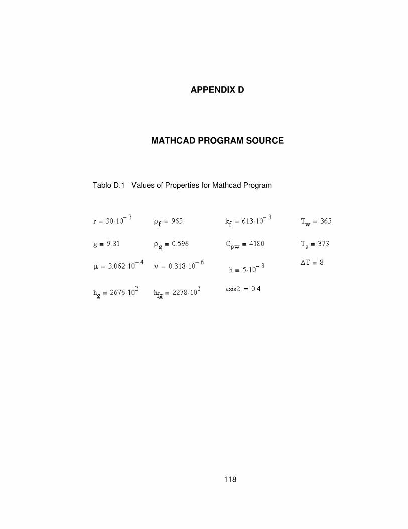
118
APPENDIX D
MATHCAD PROGRAM SOURCE
Tablo D.1 Values of Properties for Mathcad Program

119

120
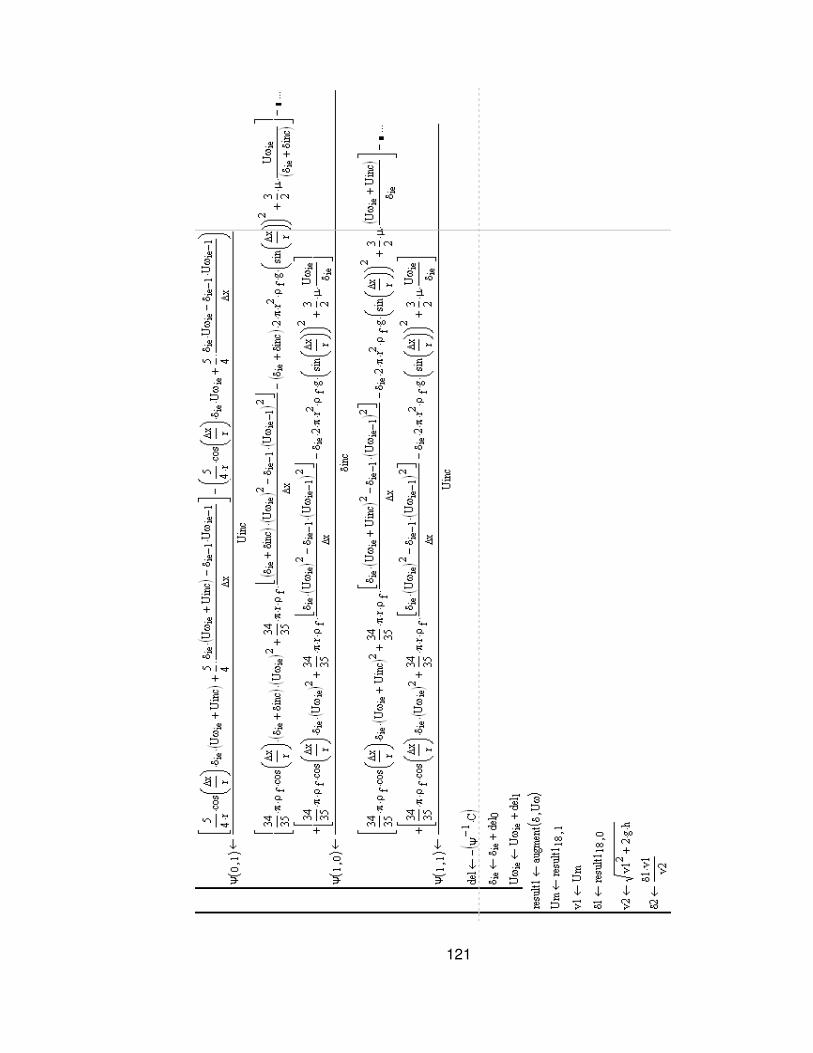
121
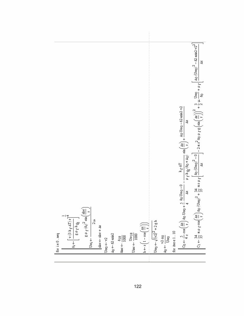
122

123

124

125
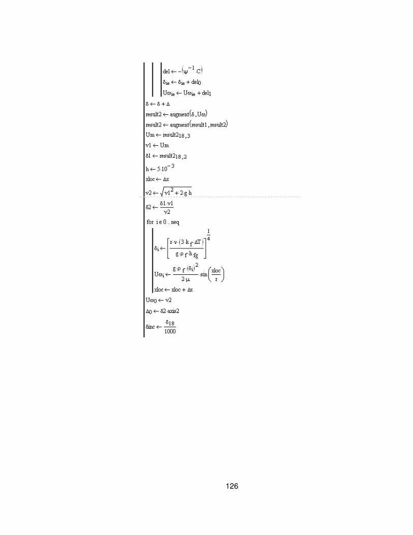
127
126
128
127
129
128


131
129

132
130

1
131