i

FEASIBILITY STUDY OF A PROTOTYPE MINIATURIZED

METABOLIC GAS ANALYSIS SYSTEM FOR MAXIMAL

EXERCISE TESTING

by

Tamara Lynn Anderson

A thesis submitted to the faculty of The University of Utah

in partial fulfillment of the requirements for the degree of

Master of Science

Department of Bioengineering

The University of Utah

December 2010

ii

Copyright © Tamara Lynn Anderson 2010

All Rights Reserved

ii

T h e U n i v e rs i t y o f U ta h Gra dua te S cho o l

STATEMENT OF THESIS APPROVAL

The thesis of Tamara Lynn Anderson

has been approved by the following supervisory committee members:

Dwayne Westenskow , Chair 10/25/2010

Date Approved

Joseph Orr , Member 10/14/2010

Date Approved

Rob MacLeod , Member 10/25/2010

Date Approved

and by Richard D. Rabbitt , Chair of

the Department of Bioengineering

and by Charles A. Wight, Dean of The Graduate School.

iii

ABSTRACT

Metabolic gas analysis systems are important devices that are used to analyze

respiratory gas exchange including volumetric flow rates and oxygen and carbon dioxide

concentrations. This information provides useful insights into metabolic function.

Traditionally, these systems were limited by their size and the functional requirements of

the gas sensors including its sensitivity to water vapor and the alignment of flow and gas

signals for real time analysis. Recently, Phillips-Respironics has developed a novel

oxygen sensor that utilizes luminescence technology for oxygen analysis. When

combined with a differential-pressure transducer and an on-airway nondispersive infrared

CO2 sensor, the result is a compact system suitable for real time breath-by-breath gas

analysis. The system has been validated for use in a critical care environment with low

respiratory flows of ±180 L/min. The purpose of this study was to determine the

feasibility by modifying the existing breathing circuit to accommodate higher volumetric

gas flows (±400 L/min) for exercise stress testing applications.

Several variations of the prototype systems were constructed. To increase the

flow, a differential pressure flow transducer was obtained from a commercially available

system used for exercise testing. The gas analysis sensors were then inserted into the

main lumen at a 45o angle so that the signal strength across the differential pressure drop

was greater than 5 cm H2O at 400 L/min and produced minimal back pressure resistance.

iv

Characterization of the flow required the use of a flow coefficient, indexed by the

Reynolds number, to adjust for head losses created by the differential pressure sensor.

With the flow coefficient adjustments, the accuracy of the flow compared to the

theoretical flow value was within ±3% or ±1 L. A propane combustion chamber that

simulated oxygen consumption was used to validate the luminescence-quenching oxygen

sensor. The fraction of expired oxygen was determined theoretically based on the

complete combustion of propane and compared to the actual recorded valued. The sensor

was found to be accurate to within 6% across the range of flow.

TABLE OF CONTENT ABSTRACT ....................................................................................................................... iii

ACKNOWLEDGEMENTS .............................................................................................. vii

Chapter 1. INTRODUCTION ....................................................................................................... 1

1.1. Objectives ............................................................................................................. 1

1.2. Applications of Respiratory Gas Analysis ........................................................... 2

1.3. Gas Analysis Techniques ..................................................................................... 3

1.4. Limitations of Current Systems ........................................................................... 8

1.5. Innovation of Luminescence Quenching Oxygen Sensor .................................... 9

1.6. Motivation for Development of a Portable Metabolic System .......................... 11

1.7. Exercise Stress Testing....................................................................................... 12

1.8. Overview of Thesis ............................................................................................ 14

2. PROTOTYPE DESIGN ............................................................................................ 16

2.1. Introduction ........................................................................................................ 16

2.2. Description of Terminology ............................................................................... 17

2.3. Prototype Design Criteria ................................................................................... 18

2.4. Materials and Methods ....................................................................................... 19

2.5. Results ................................................................................................................ 22

2.6. Discussion .......................................................................................................... 24

3. CALIBRATION OF THE DIFFENTIAL PRESSURE FLOW SENSOR ................ 44

3.1. Introduction ........................................................................................................ 44

3.2. Materials and Methods ....................................................................................... 45

vi

3.3. Results ................................................................................................................ 54

3.4. Discussion .......................................................................................................... 56

4. VALIDATION OF LUMINESCENCE QUENCHING OXYGEN SENSOR ......... 65

4.1. Introduction ........................................................................................................ 65

4.2. Materials and Methods ....................................................................................... 66

4.3. Results ................................................................................................................ 71

4.4. Discussion .......................................................................................................... 73

5. CONCLUSIONS ....................................................................................................... 80

5.1. Summary of Results ........................................................................................... 80

5.2. Future Work ....................................................................................................... 83

5.3. Possible Applications ......................................................................................... 84

REFERENCES ................................................................................................................. 86

vii

ACKNOWLEDGEMENTS

I would like to thank all those who have supported me in this endeavor. First, my

committee members Dr. Dwayne Westenskow, Dr. Joseph Orr, and Dr. Rob MacLeod.

Thank you for providing me with the opportunity to continue my education by providing

the funding for the project and allowing me to work under your direction. Second, to all

of my coworkers in the lab. Thank you for answering my endless questions and sharing

your knowledge, especially of Matlab, with me. And third, to my wonderful friend and

family. Thank you for encouraging me to pursue this degree and providing me with

strength and support during the process. I love you all!

1

CHAPTER 1

1. INTRODUCTION

INTRODUCTION

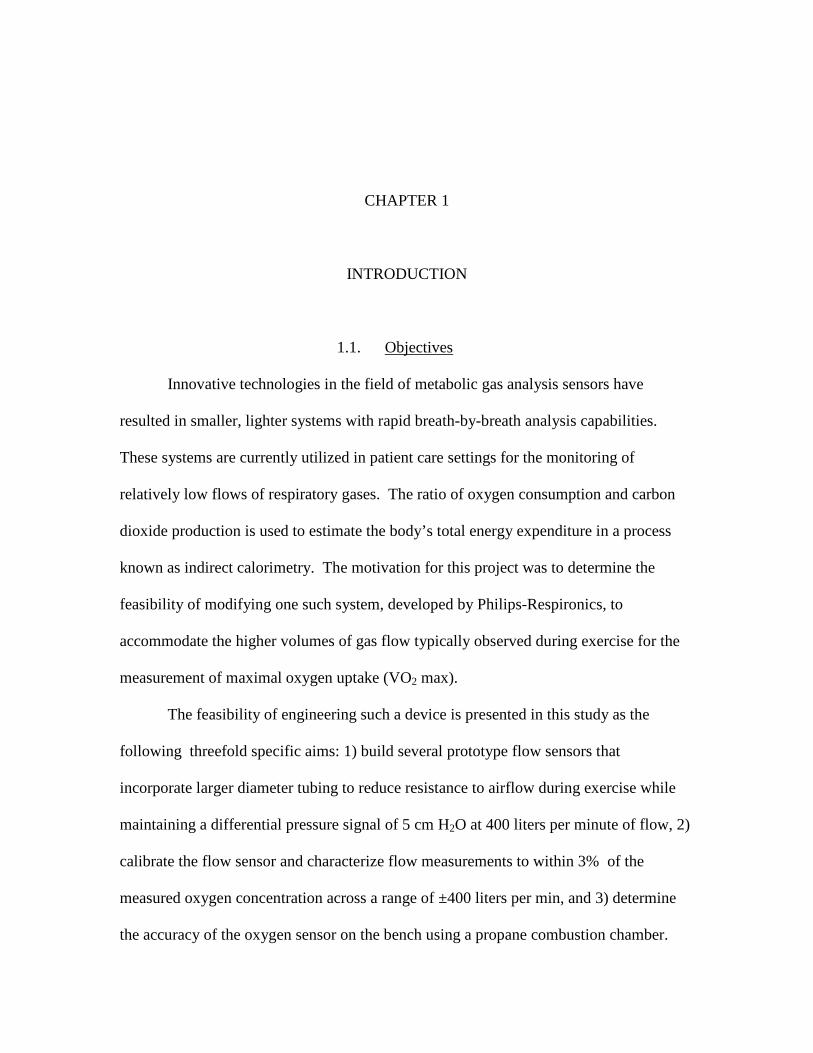
1.1. Objectives

Innovative technologies in the field of metabolic gas analysis sensors have

resulted in smaller, lighter systems with rapid breath-by-breath analysis capabilities.

These systems are currently utilized in patient care settings for the monitoring of

relatively low flows of respiratory gases. The ratio of oxygen consumption and carbon

dioxide production is used to estimate the body’s total energy expenditure in a process

known as indirect calorimetry. The motivation for this project was to determine the

feasibility of modifying one such system, developed by Philips-Respironics, to

accommodate the higher volumes of gas flow typically observed during exercise for the

measurement of maximal oxygen uptake (VO2 max).

The feasibility of engineering such a device is presented in this study as the

following threefold specific aims: 1) build several prototype flow sensors that

incorporate larger diameter tubing to reduce resistance to airflow during exercise while

maintaining a differential pressure signal of 5 cm H2O at 400 liters per minute of flow, 2)

calibrate the flow sensor and characterize flow measurements to within 3% of the

measured oxygen concentration across a range of ±400 liters per min, and 3) determine

the accuracy of the oxygen sensor on the bench using a propane combustion chamber.

2

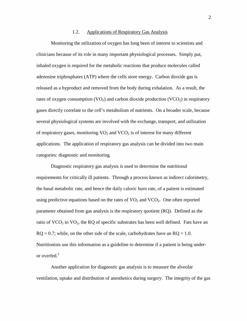
1.2. Applications of Respiratory Gas Analysis

Monitoring the utilization of oxygen has long been of interest to scientists and

clinicians because of its role in many important physiological processes. Simply put,

inhaled oxygen is required for the metabolic reactions that produce molecules called

adenosine triphosphates (ATP) where the cells store energy. Carbon dioxide gas is

released as a byproduct and removed from the body during exhalation. As a result, the

rates of oxygen consumption (VO2) and carbon dioxide production (VCO2) in respiratory

gases directly correlate to the cell’s metabolism of nutrients. On a broader scale, because

several physiological systems are involved with the exchange, transport, and utilization

of respiratory gases, monitoring VO2 and VCO2 is of interest for many different

applications. The application of respiratory gas analysis can be divided into two main

categories: diagnostic and monitoring.

Diagnostic respiratory gas analysis is used to determine the nutritional

requirements for critically ill patients. Through a process known as indirect calorimetry,

the basal metabolic rate, and hence the daily caloric burn rate, of a patient is estimated

using predictive equations based on the rates of VO2 and VCO2. One often reported

parameter obtained from gas analysis is the respiratory quotient (RQ). Defined as the

ratio of VCO2 to VO2, the RQ of specific substrates has been well defined. Fats have an

RQ = 0.7; while, on the other side of the scale, carbohydrates have an RQ = 1.0.

Nutritionists use this information as a guideline to determine if a patient is being under-

or overfed.1

Another application for diagnostic gas analysis is to measure the alveolar

ventilation, uptake and distribution of anesthetics during surgery. The integrity of the gas

3

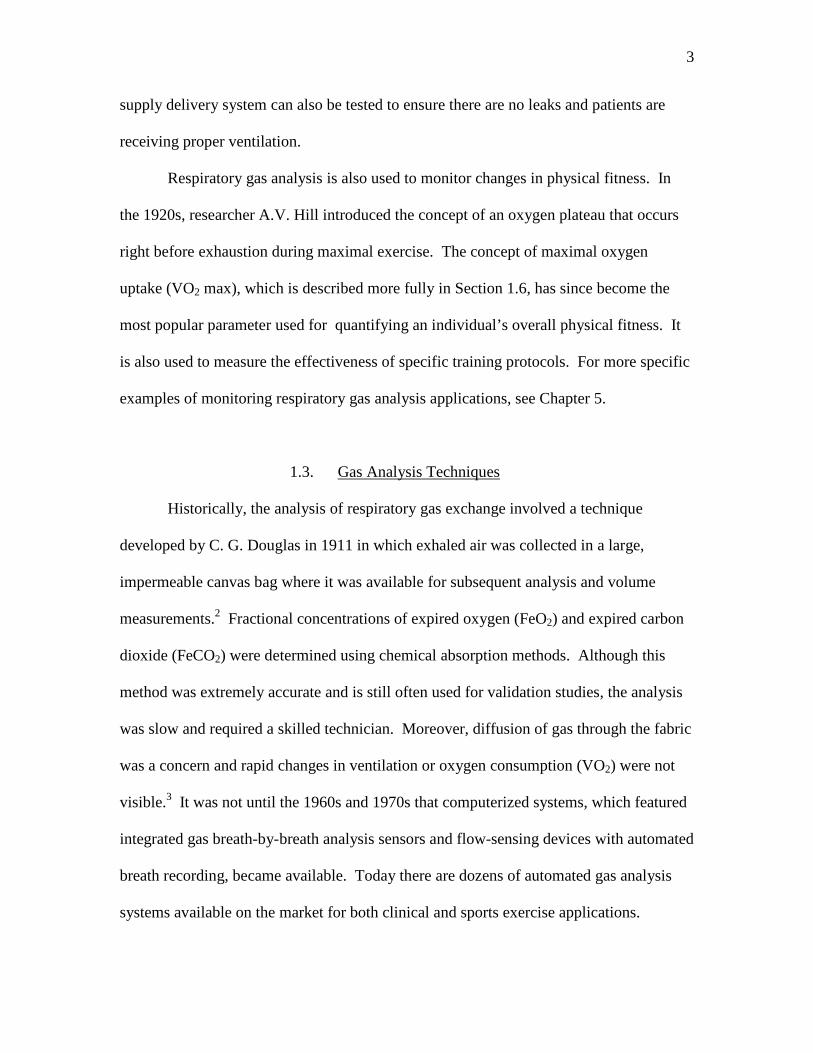
supply delivery system can also be tested to ensure there are no leaks and patients are

receiving proper ventilation.

Respiratory gas analysis is also used to monitor changes in physical fitness. In

the 1920s, researcher A.V. Hill introduced the concept of an oxygen plateau that occurs

right before exhaustion during maximal exercise. The concept of maximal oxygen

uptake (VO2 max), which is described more fully in Section 1.6, has since become the

most popular parameter used for quantifying an individual’s overall physical fitness. It

is also used to measure the effectiveness of specific training protocols. For more specific

examples of monitoring respiratory gas analysis applications, see Chapter 5.

1.3. Gas Analysis Techniques

Historically, the analysis of respiratory gas exchange involved a technique

developed by C. G. Douglas in 1911 in which exhaled air was collected in a large,

impermeable canvas bag where it was available for subsequent analysis and volume

measurements.2 Fractional concentrations of expired oxygen (FeO2) and expired carbon

dioxide (FeCO2) were determined using chemical absorption methods. Although this

method was extremely accurate and is still often used for validation studies, the analysis

was slow and required a skilled technician. Moreover, diffusion of gas through the fabric

was a concern and rapid changes in ventilation or oxygen consumption (VO2) were not

visible.3 It was not until the 1960s and 1970s that computerized systems, which featured

integrated gas breath-by-breath analysis sensors and flow-sensing devices with automated

breath recording, became available. Today there are dozens of automated gas analysis

systems available on the market for both clinical and sports exercise applications.

4

These automated gas analysis systems employ various techniques for determining

gas concentrations including mass spectrometry and substance sensitive sensors and

detectors. The purpose of this section is to provide an overview of the technologies and

discuss the applications and limitations of the different methods. It should be noted that

the words sensor and detector are used interchangeably throughout this report.

1.3.1. Mass Spectrometry

Mass spectrometry (MS) is an analytical technique for determining the

composition of a sample based on the masses of individual molecules. Mass

spectrometers consist of an ion source, a mass analyzer, and a detector. First, the sample

is loaded into the instrument where it is vaporized to form a gas. Then the sample is

bombarded with an electrical beam that causes ions to form. Because ions are extremely

reactive and short-lived, their formation is conducted in a vacuum. An electrical field is

then applied to the sample, which causes the cations, formed in the previous step, to

accelerate towards an electrode. Another perpendicular magnetic field deflects the ions.

Based on the deflection trajectory pattern, the mass analyzer determines the mass-to-

charge ratio of the sample.

Finally, the sample is collected by the detector and the ion flux is converted to a

proportional electrical current. The information is converted into a mass spectrum and

can be used to determine the concentrations of each species present. MS is capable of

detecting very minute quantities (one part per billion). 4-6

5

1.3.2. Metabolic Gas Analyzers

Metabolic gas analysis systems, or metabolic carts, are used to indirectly estimate

energy expenditure through the continuous monitoring of respiratory gases.7 In exercise

physiology the measurements of VO2 and VCO2 are used to assess aerobic capacity

during maximal exercise. In a clinical setting metabolic carts are often used to obtain

information about gas exchange for anesthesia and to determine calorie requirements for

bedridden patients.

These systems must be inexpensive, lightweight, robust, easily calibrated, simple

to operate, and reliable. Unlike the Douglas bag method, modern metabolic gas analyzers

are able to provide breath-by-breath analysis. Common features of all the devices include

a spirometers for the measurement of gas flow, a carbon dioxide detector, and an oxygen

sensor.8 A brief description of the components is provided in the following sections.

1.3.2.1. Spirometers. Spirometers are used to measure lung function,

specifically the volume or flow related to respiration as a function of time (m3/s). This

can be determined directly using traditional volume spirometers, or indirectly using a

flow detector which derives the volume mathematically.

Direct spirometery records the rotation of a diaphragm when a breath is forcibly

exhaled. The movement is traced on a moving paper graph where the volume is

measured. There are three types of standard spirometers: the water seal, dry rolling seal,

and bellow spirometers. Since spirometers are often large in mass, their use is

impractical when measuring rapid changes in volume. For this reason they are not

typically used for maximal exercise stress tests.9

6

For the indirect measurement of flow devices known as pneumotachometers are

often used. Pneumotachometers rely on the principle that a drop in pressure is directly

proportional to gas flow.10 A computer integrates the flow over time to produce a gas

volume. It should be mentioned there are four main types of pneumotachometers used in

automated metabolic systems: differential pressure, turbines, Pitot tubes, and hot-wire

anemometers. However, a further description of the different types is beyond the scope

of the report. They are relatively inexpensive and can be disposable. While some

criticize this method because volume is not measured directly, pneumotachometers are

more robust and respond rapidly to changes in air flow, making them more suitable for

exercise studies.

1.3.2.2. Carbon dioxide detector. Non-Dispersive infrared (NDIR) detectors are

the most widely used method for the real-time measurement of carbon dioxide. Carbon

dioxide absorbs infrared radiation at a specific wavelength due to the fundamental

asymmetric O=C=O stretch. The sensor consists of an infrared (IR) source and a

detector. Absorbance of the infrared light at 4.26 microns is proportional to the

concentration of carbon dioxide. Most systems also have a reference signal, which

detects the amount of light at a different wavelength where there is no absorbance.11

1.3.2.3. Oxygen sensor. Currently three main technologies are used in

metabolic carts for oxygen concentration analysis: 1) semidisposable electrochemical

sensors, 2) paramagnetic sensors, and 3) zirconium oxide oxygen sensors. A brief

description of the technology is provided below.

Semidisposable electrochemical sensors use a galvanic fuel cell or polarographic

(Clark) electrode to produce a stable current that is proportional to the partial pressure of

7

oxygen. These fuel cells have the advantage of being small, which makes them desirable

for portable systems. The use of galvanic sensors in metabolic carts has been limited

because they do not respond rapidly to changes in concentration, are expensive, and have

a short electrode lifetime especially when exposed to high concentrations of oxygen.

Polarographic sensors have a longer storage life than galvanic sensors, but require a

significant amount of maintenance and upkeep.12, 13

Zirconium oxide fuel cells consist of a calcium-stabilized zirconium oxide

electrolyte with porous platinum electrodes. At high temperatures (770-850 oC), the

zirconium lattice becomes porous and conducts the movement of oxygen ions from a

higher concentration to a lower concentration. Typically one electrode is exposed to air

and the other is exposed to the sample gas. The output voltage follows the Nernst

equation and is relative to the partial pressure of oxygen. The sensor is extremely stable,

precise over a wide range from 100% oxygen down to parts per billion, and capable of a

fast response time. One major limitation is sensor fatigue, which results from the heating

and cooling of the sensor. Also, at high temperatures, reducing gases (hydrocarbons of

another species, hydrogen, and carbon monoxide) react with oxygen to produce a lower

than actual oxygen reading.14

In a paramagnetic sensor, the magnetic susceptibility of oxygen is used to

determine the partial pressure. In the 1800s Michael Faraday noted that the oxygen in a

gas sample caused the rotation of a nitrogen-filled glass dumb-bell suspended in a

magnetic field. The current needed to counteract the rotation is proportional to the

concentration of oxygen. Today the systems consist of a light source, photodiode, and an

amplifier circuit, which is used to measure the degree of rotation of the dumbbell. The

8

dumbbell is filled with an inert gas and suspended within a nonuniform magnetic field.

When oxygen is present, the molecules are attached to the electromagnetic field and the

dumbbell rotates. In addition to fast response times and the absence of consumable parts,

the sensor has a good shelf life, making it the most utilized oxygen sensor. However, this

method is not sensitive to trace amounts of oxygen.15,16

1.4. Limitations of Current Systems

In the 1980s and early 1990s mass spectrometers went from complex instruments

that filled entire rooms to user-friendly bench-top devices. Further miniaturizing mass

spectrometers has conventionally been limited by the vacuum and pump requirements.

The ionization requirement destroys the sample, which is not desirable for all

applications. Although there is rising interest in portable mass spectrometers for field

studies, major manufacturers are concerned about limited markets and profit margins.

Thus, mass spectrometers have remained relatively expensive when compared to

metabolic gas analyzers.17

Computerized metabolic gas analyzers are often preferred over the Douglas bag

technique because they can provide breath-by-breath information about gas exchange.

However, several studies have shown there is wide variability in the reported parameters

by the metabolic gas analyzers and there is still some debate about their accuracy. In a

review of the automated systems, Macfarlane (2001) points out that these systems still

have several shortcomings.8

First, the automated systems no longer require the user to have an understanding

of how the data is generated. This creates conceptual and technical problems during data

9

analysis. Second, oxygen and carbon dioxide sensors are sensitive to the presence of

water vapor. Water vapor can condense in the sampling line where it must be removed

before it reaches the sensor. Another challenge is keeping the partial pressure of water

vapor the same during the calibration and measurement phases to obtain the correct

results for dry gas concentrations.

The third problem, which Macfarlane suspects is the greatest of the three, is that

the automated systems require an exact alignment of the flow and gas analysis signals.

Many systems utilize a mixing chamber for steady-state gas analysis. This method

creates a lag between the gas analysis signal and the flow signal, which must be realigned

for breath-by-breath analysis.

1.5. Innovation of Luminescence Quenching Oxygen Sensor

Recently Phillips-Respironics (Phillips, Carlsbad, California) introduced an

innovative technique, based on the principle of luminescence quenching, for the

measurement of oxygen to be used in their clinical metabolic cart known as the NICO

Respiratory Profile Monitor.

The instrument consists of a light emitting diode that serves as the excitation

source for a luminescent dye. A photosensitive detector is mounted in a position to

respond to the filtered fluorescent radiation emerging from the exit optical filter. The

oxygen sensor, contained in a cuvette along with a NDIR CO2 analyzer, is comprised of a

thin film of transparent material containing the luminescent dye where rapid diffusion of

molecular oxygen from the airway gas environment takes place. The system is more

rapidly depleted of the excited-state dye molecules when oxygen is present, making the

10

oxygen concentration proportional to the amount of quenching observed. Simply, when

oxygen is not present in the system, more fluorescence is observed than when oxygen is

present in the system.

A short pulse of light illuminates the film 100 times a second and the system

analyzes the magnitude and phase of the resulting excitation following each pulse. Each

pulse provides a sample of the oxygen signal. This oxygen signal is presently designed to

give a simple oxygen waveform and measurement of inspired and expired oxygen with

the existing flow signal to calculate oxygen uptake.

The accuracy of the luminescence quenching technique for oxygen analysis in a

critical care environment was performed in the lab using a patient lung simulator.

Through the combustion of propane, which occurs in a sealed chamber, the exact amount

of VO2 and VCO2 and water vapor production can be determined. When compared with

the oxygen consumption measured by the sensor, the accuracy was found to be within -

0.3±2.8%.18

Further validation of the sensor was performed in a clinical trial using 20 (10

female, 10 male) human volunteers at rest. When compared against the clinical gold

standard device (DeltaTrac, Datex, Helsinki, Finland) an error in oxygen consumption

measurement of 2.2±4.1% and an error 1.63±4.41% in carbon dioxide production

measurement was found.19 The system was also tested on 14 intensive care unit (ICU)

patients and found to be within 1.7±6.9% of the reference analyzer.20

In a clinical setting with respiratory gas flows of less than ±180 L/min, this novel

sensor offers many advantages over previous methods for determining oxygen

concentration. The sensor can be placed directly on the airway instead of a side stream

11

so that real-time oxygen consumption is possible. This eliminates the need for aligning

the flow and breath signals and water condensation in the hoses of the drawn sample.

Due to its light sensitive properties, the sensor is subjected to photo bleaching over time.

However, the sensors are relatively cheap and are not difficult to replace.

1.6. Motivation for Development of a Portable Metabolic System

Up to this point the utilization of luminescence quenching technology has been

primarily focused on its benefits in metabolic analysis systems in a clinical setting, but

there is a growing demand for a portable gas analysis system to be used as part of a

routine health monitoring. Once only a small portion of athletes used exercise stress

testing to determine their fitness levels. Now every day exercise enthusiasts are

interested in parameters obtained from gas analysis, primarily maximal oxygen uptake.

Similarly, popular televisions shows that feature gas analyses as a way to determine and

track daily energy expenditure have increased the demand for gas analysis as a weight

loss tool. While there are a few portable gas analysis systems available, most rely on

galvanic fuel cells for oxygen analysis. The purpose of this research is to extend the use

of luminescence quenching technology by developing a prototype metabolic system that

could be used during exercise testing.

The following section provides an overview of exercise stress testing including

the definition of maximal oxygen uptake, how it is determined, and the expected ranges

for different athletes. As discussed earlier, the determination of energy expenditure is

straightforward based on the ratio of oxygen consumption to carbon dioxide production.

12

1.7. Exercise Stress Testing

1.7.1. Maximal Oxygen Uptake (VO2 Max)

The most commonly measured parameter during exercise stress tests is maximum

oxygen uptake (VO2 max). During exercise, the several physiological systems must work

together in order to provide the body with the nutrients, including oxygen for the

production of ATP, needed to sustain the activity. At some point during maximal

exercise the linear relationship between O2 consumption and mechanical power plateaus.

This point, known as VO2 max, is considered the best indicator of cardiorespiratory

endurance and aerobic fitness. Consequently, measuring VO2 max is of interest to

athletes and others seeking to monitor their cardiovascular fitness.

Maximal oxygen uptake is largely influenced by three major factors: cardiac

output, the oxygen carrying capacity of the blood, and the amount of exercising skeletal

muscles and the ability of those muscles to utilize the supplied oxygen.21 Other factors

include age, gender, altitude, and overall physical health. Some estimates say that

genetics and heredity account for nearly 25-50% of the variance in VO2 seen between

individuals.22,23 Some of these factors do not change with exercise, but endurance

training can greatly increase the ability of aerobic enzymes to extract oxygen from the

blood.24 The type of muscle fiber is also important. Briefly, slow twitch muscle fibers

are naturally more oxidative, and have more mitochondria and capillaries than the fast

twitch muscle fibers developed during strength training. This allows the muscles to

better utilize the oxygen from the blood.25

13

1.7.2. Measurement

To determine the VO2 max, respiratory gas flow and the concentration of inspired

and expired oxygen and carbon dioxide must be recorded simultaneously while the

subject is performing a specific exercise protocol. The breathing circuit is attached to a

headpiece, which must be worn during the exercise test. Room air, which contains

20.93% oxygen and 0.03% carbon dioxide, is inhaled through a non-rebreathing valve.

When the subject exhales, the gas travels through the breathing circuit to a metabolic cart

where gas analysis occurs. After the concentration of oxygen in the inspired air is

adjusted for barometric pressure, humidity, and temperature, oxygen consumption can be

determined.

The classic protocol for VO2 max testing involves exercising on a treadmill or

stationary ergometer. The intensity of the work load increases at periodic intervals until

the subject is exhausted and cannot continue. This usually occurs after about 10-15

minutes of exercise. A true VO2 max reading requires a trained test administrator and a

highly motivated individual. Sometimes there is not a clear plateau observed. In these

cases, secondary criteria including high levels of lactic acid in the blood, an elevated

respiratory exchange ratio, and some percentage of an age-adjusted maximal heart rate

are used to determine the exact point of VO2 max. VO2 max can also be estimated using

predictive equations based on heart rate and work rate.

1.7.3. Average Range for Normal Individuals

Because oxygen and energy requirements vary with body type and size, VO2 max

is often expressed in ml O2/kg/min. A typical human at rest requires 3.5 ml O2/kg/min

14

for just for cellular activities. The average VO2 max for an untrained 40 year old male is

in the range of 35-40 ml O2/kg/min. In general, a female of the same age would have a

value around 30-35 ml O2/kg/min. By contrast, cyclist Lance Armstrong has a reported

VO2 max of 83-85 ml/kg/min; Steve Prefontain, an elite runner; 84.4 ml/kg/min; Bjorn

Daehlie, a Norwegian cross country skier, 90.0 kg/ml/min; and female marathon runner

Joan Benoit, 78.6 ml/kg/min. A Scandinavian cross country skier is reported to hold the

record for the highest VO2 max at 94 ml/kg/min.26

1.8. Overview of Thesis

The ultimate goal of this project was to determine the feasibility of developing a

prototype gas analysis system that incorporated a luminescence quenching O2 sensor, a

NDIR CO2 sensor, and a fixed orifice differential pressure flow meter. Each of these

components has been successfully used individually or in combination for clinical

applications, but together the three pieces have not been used for monitoring gas analysis

applications such as exercise stress testing. To evaluate the prototype system, the project

was divided into three stages.

In the first stage, presented in Chapter 2, three criteria were established for the

design of the prototype system. Several prototype metabolic gas analysis systems with

different sensor configurations were constructed. The designs were tested to ensure that

enough gas flow reached the sensor for adequate analysis. Back pressure resistance and

flow signal were also measured. A discussion of each design and its performance is

included. The commercial requirements for back pressure resistance and flow signal are

also discussed, and the best design was selected.

15

In the second phase, Chapter 3, the flow sensor was calibrated using a correction

factor known as the discharge coefficient. The use of indirect flow measurement by

means of a fixed orifice differential pressure transducer is discussed. The derivation of

the flow equations using the Bernoulli equation and the discharge coefficient theory are

also presented. The coefficient was determined and the accuracy of the prototype flow

sensor using the discharge coefficient is given.

In the last stage, Chapter 4, the accuracy of luminescence quenching oxygen

sensor was tested on the bench using a propane combustion patient simulator. The

combustion of propane requires a fixed amount of oxygen. This amount was then

compared to the measured amount of the oxygen in the gas from the chamber by the

sensor. A discussion of the experimental design limitations concludes the research

section.

Finally, in the closing chapter the results are again summarized. Limitations of

the methods used in the study are presented including any future work that is necessary

before the prototype system could be developed commercially. A few possible

applications are suggested. A summary of the overall findings concludes the project.

16

CHAPTER 2

2. PROTOTYPE DESIGN

PROTOTYPE DESIGN

2.1. Introduction

Luminescence quenching has been used successfully in a critical care

environment. With a few modifications it was proposed that the applications could

extend to monitoring applications. As part of a collaborative effort between Phillips-

Respironics and Dr. Joseph Orr and his research group at the University of Utah, a

compact flow measurement system complete with the hardware and algorithms needed

for measurement of VO2 and VCO2 was developed. The technology is currently

marketed by Phillips under the trade name FloTrac Elite. Because of its compact size it

is ideal for a portable metabolic gas analysis system. However, its use in exercise testing

is currently limited by the diameter of the tubing and the volumetric flow it is capable of

handling. The purpose of this stage of the project was to modify the flow sensor housing

so that more airflow was available.

This chapter includes a description of the terminology used when designing the

breathing circuit, the desired criteria and methods for testing each exercise prototype

breathing circuit, the results including end-tidal CO2 (ETCO2), back pressure, and

resistance tests, and a discussion of the selected prototype and its performance. The units

of volumetric flow are given in liters per minute (L/min) and liters per second (L/s).

17

2.2. Description of Terminology

There are three main components of the prototype gas analysis system: 1) the

breathing circuit, which is made up of the on-airway luminescence quenching O2 sensor,

NDIR CO2 analyzer, and the differential pressure port housing, 2) the FloTrac Elite,

which is the module containing the algorithms required for the gas analysis, and 3) the

Capnostat, which is connected to the FloTrac Elite and acts as the excitation source and

detector for NDIR CO2 and O2 analysis.

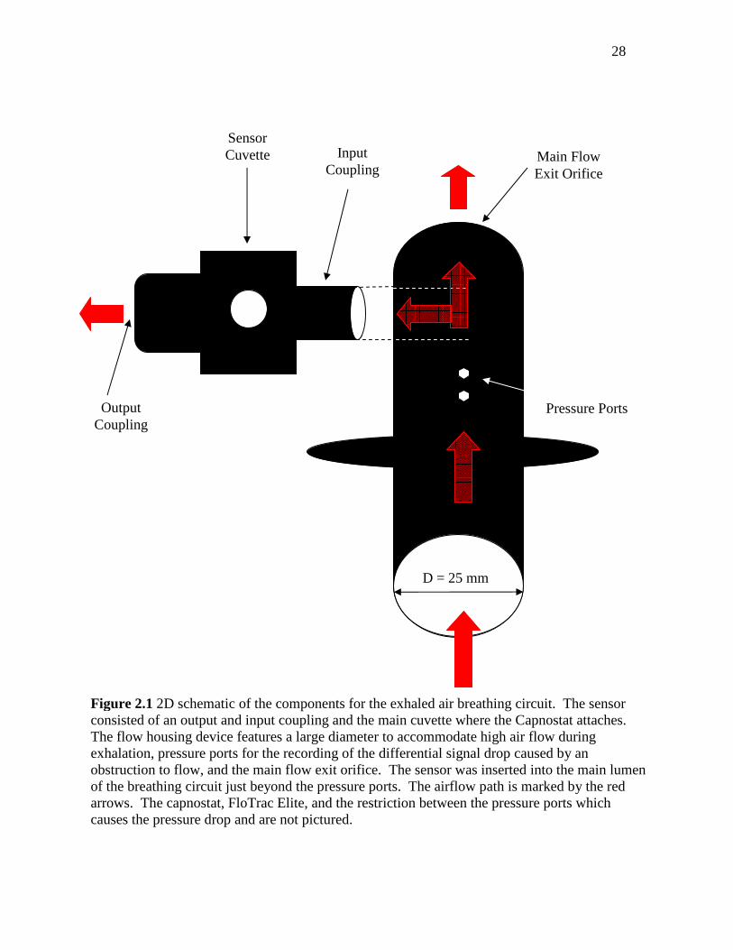
A schematic of a portion of the breathing circuit is shown in Figure 2.1. The

sensor consists of a gas cuvette with a coupling on either side. The capnostat attaches to

the cuvette. As the sampled gas travels through the cuvette the capnostat detects the O2

and CO2 molecules present and relays the information to the FloTrac Elite for signal

processing. The gas cuvette was inserted into the main lumen of the flow housing device

well after the pressure ports. The exhaled flow was then directed either out of the main

flow orifice or across the sensor.

Based on the orientation of the sensor in this study, gas flow first enters the

smaller diameter coupling (~13 mm), moves through the sampling chamber in the

cuvette, and exits the larger diameter coupling (~16 mm). Hence, each coupling will be

distinguished as the input and output coupling, respectively.

The housing for the differential pressure flow sensor was obtained from a

CardioCoach Fitness Assessment Analyzer (Korr Medical, Salt Lake City, Utah). The

oxygen and carbon dioxide sensors were provided by Phillips-Respironics (Phillips-

Respironics, Carlsbad, California). The pressure differential drop was created by a slight

constriction in the main lumen of the flow located in between the two ports. The

18

standard pressure ports included on the housing were connected via tubing to the pressure

transducer also located in the FloTrac Elite. The FloTrac Elite outputs the drop as a

volumetric flow using computer algorithms.

The gas flow path is shown in Figure 2.1 in red. Only the portion of the sensor

utilized when the subject exhales is shown. The headpiece worn by the subject and the

mask including the inhalation non-rebreathing valve is not pictured.

2.3. Prototype Design Criteria

Three criteria were considered when designing a prototype on-airway gas analysis

system. First, the expected respiratory flow for a patient in the intensive care unit (ICU)

is small – no more than 180 L/min at a maximum. Thus, only a small diameter (<15 mm)

is required for the lumen of the breathing circuit to meet the airflow requirements.

During exercise a healthy adult requires air flows in the range of 400 L/min. The

prototype breathing circuit for an exercise metabolic gas system must feature a larger

diameter lumen that is capable of handling these flows.

Modifying the sensor cuvette could have potentially damaged the integrity of the

sensor, so it was decided the best approach would be to create a branch to divert some of

the flow across the sensor and allow the remaining flow to exit with minimal resistance.

To ensure that enough gas was reaching the sensor for adequate gas analysis, the end-

tidal CO2 (ETCO2) at the test site was recorded and compared to a reference location.

The geometry which provided a minimal difference in ETCO2 would be selected.

Second, because the system uses a differential pressure type flow sensor, a

compromise between the back pressure flow experienced by the user and the magnitude

19

of the transducer signal produced from the pressure drop was required.8 For a strong

signal-to-noise ratio a large differential pressure in response to gas flow was desirable. In

industry, a differential pressure signal of at least 5 cm H2O at 6.6 L/s is considered

acceptable.

Finally, the most effective prototype would provide adequate airflow to the sensor

for gas analysis without introducing unnecessary back pressure and hence resistance,

which may lead to premature VO2 max readings. The American Thoracic Society (ATS)

issued a policy statement recommending that the upper limit for resistance and back

pressure for a monitoring spirometers at <2.5 cm H20/L/s ±14L/s over the flow range.27, 28

2.4. Materials and Methods

2.4.1. Prototype Breathing Circuits

Several prototype breathing circuits were designed using three fundamental

sensors with additional modifications made to each. A description of the three sensors

and the modifications made to each are given in Table 2.1. To prevent back diffusion

across the sensor from the output coupling, resistance in the form of addition length was

added. No further modifications were made to the outlet coupling. Thus the description

of the modification in Table 2.1 refers solely to changes made to the input coupling. The

sensor was then inserted at a 90o angle into the lumen of the flow sensing device.

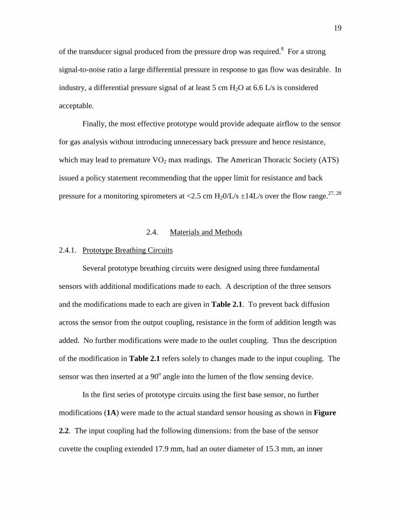
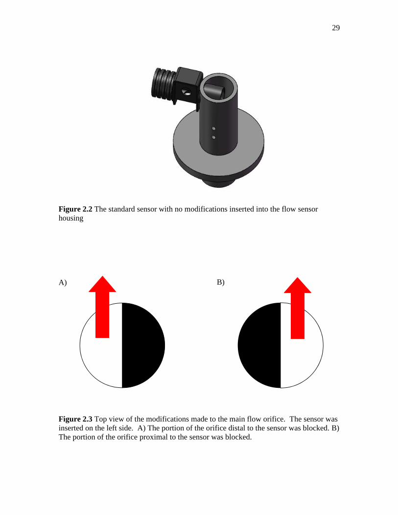
In the first series of prototype circuits using the first base sensor, no further

modifications (1A) were made to the actual standard sensor housing as shown in Figure

2.2. The input coupling had the following dimensions: from the base of the sensor

cuvette the coupling extended 17.9 mm, had an outer diameter of 15.3 mm, an inner

20

diameter of 13.3 mm, and a thickness of 1 mm. The input coupling tapered slightly so

that the circumference at the most distal portion from the base of the cuvette is 48 mm.

The additional modifications added to this series of prototypes consisted of

restrictions made to the main flow exit orifice. A schematic of the top view of the main

flow orifice opening is given in Figure 2.3. The flow paths are indicated by the red

arrows. The flow orifice proximal to the sensor was covered in the modifications 1B-1E

so that the flow was allowed to exit through the most distal opening and through the

output coupling on the sensor. In 1F-1G, the flow orifice proximal to the sensor was

uncovered and the covering was placed on the distal side.

In the second series of prototypes, the basic sensor had a 10.7 x 16.9 mm

rectangular portion of the coupling wall removed 8.4 mm from the base of the cuvette so

that the remaining circumference was 31.2 mm. The sensor was positioned in such a way

as to help direct more flow to the sensor. As in the previous series, similar modifications

to the flow orifice were made in 2B-2D. The last two modifications were an addition of

length and the remaining circumference 2E-2F. A rendition of the Sensor #2 and the last

two modifications is given in Figure 2.4.

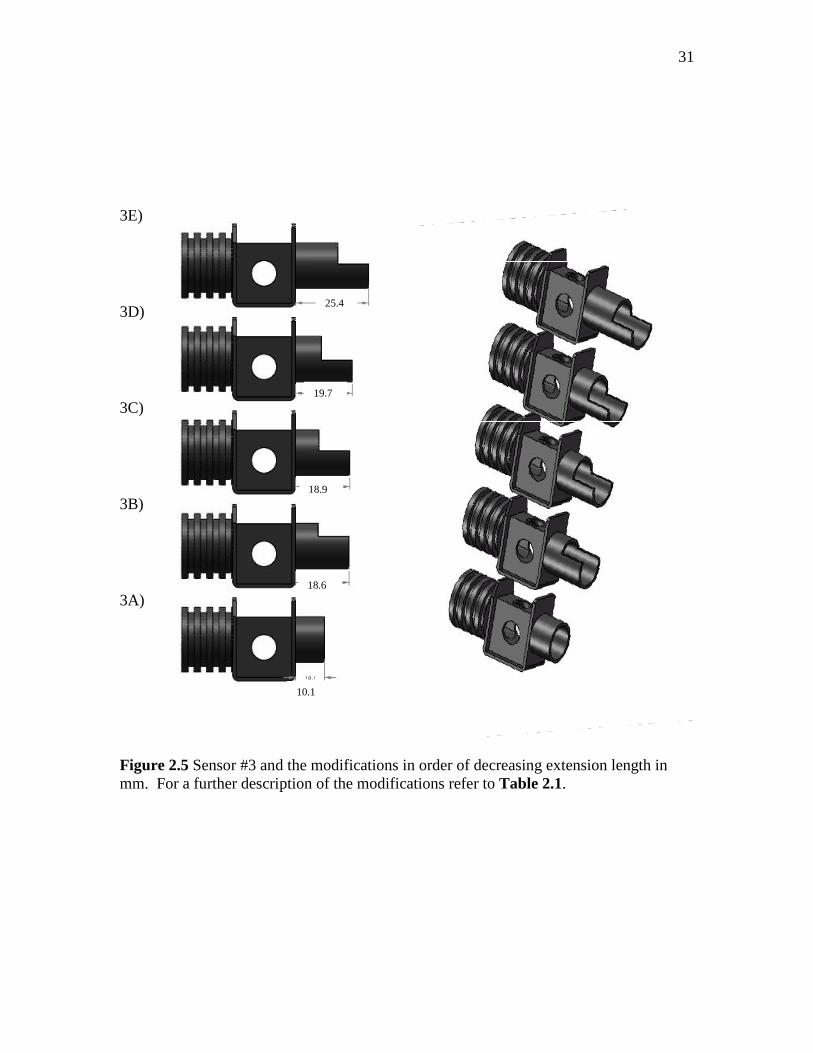
For the base sensor in the third series of prototypes, the extension of the input

coupling on a standard sensor was shortened. Then various modifications were made to

the extension and circumference as outlined in Table 2.1. Figure 2.5 shows a rendition

of the sensors arranged by the length of the extension (from the most to the least).

Based on the results of the all three series of prototypes, a final base sensor with a

25.4 mm extension to the inlet coupling was inserted into the flow at a 45o angle. A

rendition of this prototype is included in the results portion.

21

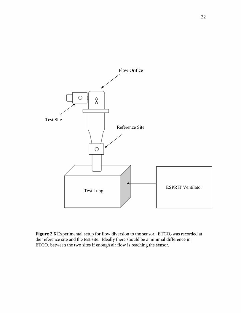
2.4.2. Flow Diversion – End-Tidal CO2

To determine the efficacy of the each design, each prototype was connected to a

test lung, Figure 2.6. At the base of the test lung was a reference sensor. The lung was

powered with an ESPRIT ventilator (Phillips-Respironics, Carlsbad, California), with the

settings shown in Table 2.2. Carbon dioxide levels were set so that the end-tidal carbon

dioxide (ETCO2) was between 34-36 mm Hg, within an acceptable range for human

ETCO2. The mechanical lung provided a tidal volume for each breath of 1 liter.

Flow Host software was used to record the flow parameters. After a one-minute

stabilization period the ETCO2 was recorded for five breaths on the reference sensor.

The process was repeated for the test site and again at the reference site.

2.4.3. Signal Strength and Back Pressure Resistance

A sensor design that met the aforementioned ETCO2 criteria was selected. The

sensor was then tested to ensure that a user would experience minimal back pressure

resistance when breathing through the circuit and that the differential pressure drop

produced a strong signal. For a baseline reference, the standard housing for the

differential pressure flow sensor obtained from Korr Medical was also tested. The

experimental setup is shown in Figure 2.7. Constant air flow at ambient conditions was

provided by an ESPRIT Ventilator (Phillips-Respironics, Carlsbad, California). The

ventilator was connected to the high flow input on a VT Plus Gas Flow Analyzer (Bio-

Tek, Winooski, Vermont), which was used to verify the flow rate. The VT Plus was

calibrated using a 3 liter syringe. The flow sensor was connected to the high flow

exhaust on the VT Plus. The sensor was connected to the FloTrac Elite and then to a

22

laptop. NICO Data collection software recorded differential pressure signal. The

average flow ranged from 2-300 L/min.

2.5. Results

2.5.1. Flow Diversion – End-Tidal CO2

The ETCO2, given in mm Hg, for the reference, test, and reference sites for each

base sensor and its modifications are presented. For a description of each base sensor and

its modifications refer to Table 2.1. The percent error, defined as the difference between

the test site and the average of both reference sites over the average of both reference

sites for the measured ETCO2 (mm Hg), is given in the last column.

For the first series, the ETCO2 measurements are given in Table 2.3 and Figure

2.8. When no modifications were made to the sensor an ETCO2 measurement could not

be obtained. When a covering was placed over the main flow orifice so that all the air

was forced the sensor, the ETCO2 at the reference site measured higher than at the test

site. When the flow orifice was only partially covered proximal to the sensor so that

some air flow was allowed to pass through the distal side of the flow orifice, a similar

pattern was observed. When the cover was moved to the distal side so that the air flow

could pass proximal to the sensor the test ETCO2 measured higher than at the reference

site.

In the second series a portion of the inlet coupling was removed. This was

thought to help lower back pressure resistance and promote gas flow to the sensor, Table

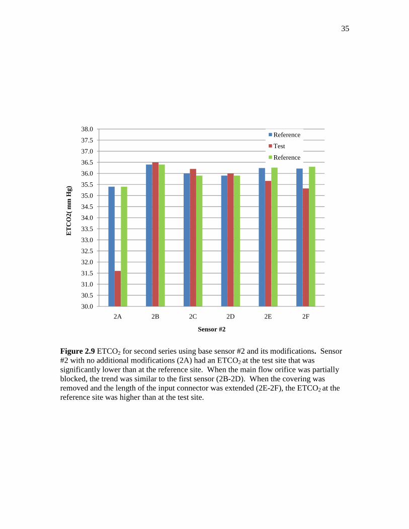
2.4 and Figure 2.9. With no modifications, the base Sensor #2 had a significantly lower

reading at the test site than the reference site. When portions of the flow orifice were

23

covered the results were similar to the first series. Once the covering was removed and

the inlet coupling was extended further into the flow housing lumen, the reference

readings increased and the test site readings decrease.

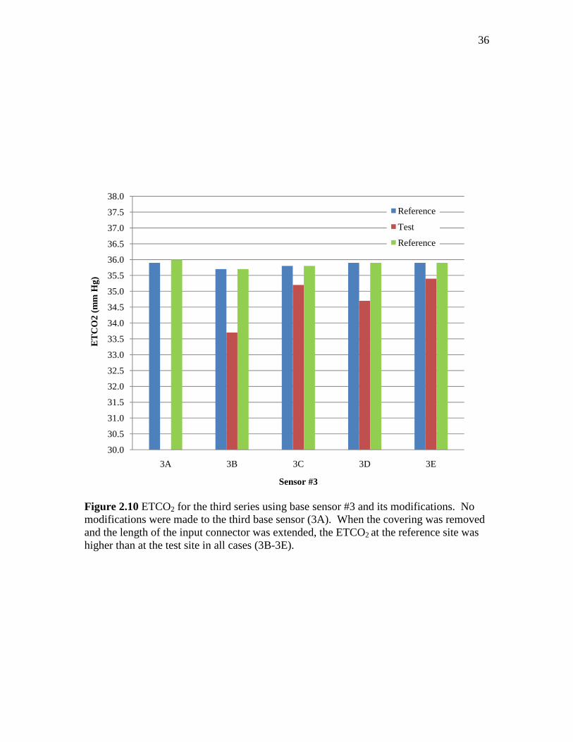
A third series of sensors using the base sensor #3 with a shorted input connector

were tested. The ETCO2 reading between the test and reference site seemed to be a

function of the extension added to the input connector, Table 2.5 and Figure 2.10. As

length was added the difference between the reference and test site ETCO2 measurements

decreased.

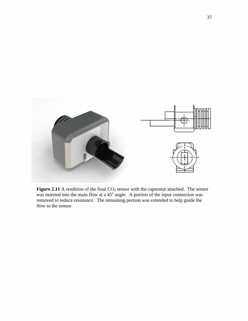
A rendition of the final sensor with the capnostat attached is shown in Figure

2.11. To optimize the possible length extension a sensor was inserted at a 45o angle into

the main flow. A portion of the input connector wall was removed to facilitate air flow

across the senor and an extension to the inlet coupling of 7.52 mm (25.4 mm from the

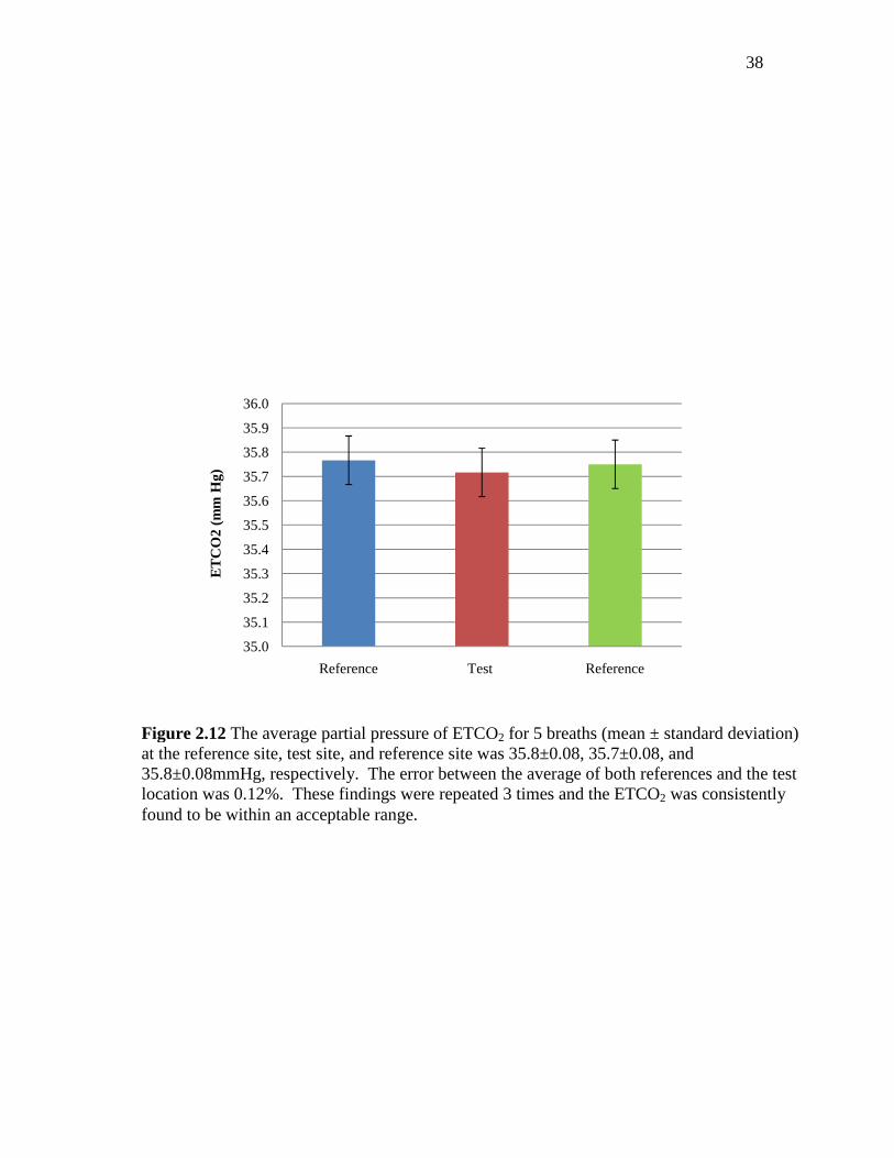
base) was added. When the ETCO2 of this sensor was tested there was a minimal

difference between the reference site and the test site, Figure 2.12. The average partial

pressure of ETCO2 for 5 breaths (mean ± standard deviation) at the reference site, test

site, and reference site was 35.8±0.08, 35.7±0.08, and 35.8±0.08 mmHg, respectively.

These findings were repeated 3 times and the ETCO2. The standard error between the

test and reference location was 0.12%.

2.5.2. Differential Pressure Signal Strength

All analysis was conducted using Microsoft Excel 2003. The VT Plus was

calibrated using a 3 liter syringe and found to have a percent error of ± 0.83%. All

experiments were conducted at ambient conditions (room temperature = 75.9, relative

24

humidity = 20%, barometric pressure = 635 mm Hg). By the National Institute of

Standards Technology’s (NIST) definition of standards conditions, a temperature of 20oC

and pressure of 760 mm Hg were used in the calculations.

The differential pressure signal (cmH2O) was recorded at flow rates of 0 to 300

L/min, Figure 2.13. The standard differential pressure housing was tested on flow rates

from 0 to 165 L/min, and is referred to in Figure 2.13 as the baseline. At low flows

differences in the baseline and modified breathing circuit differential pressure signal

strength are minimal. As the volumetric flow rate was increased the differential signal

strength improved in the modified breathing circuit.

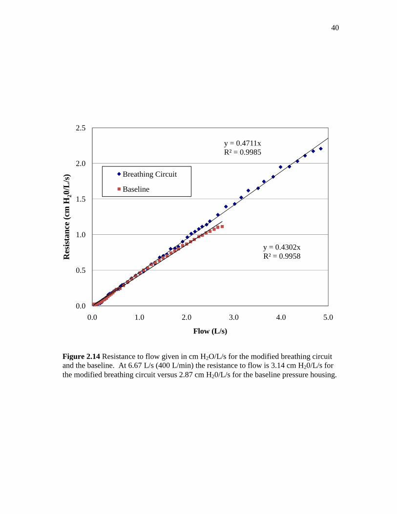
The back pressure resistance (cm H20/L/s) that a user would experience is given

in Figure 2.14. Again, at low flows deviations in the baseline and modified breathing

circuit resistance are minimal. However, as the flow increased the back pressure

resistance in the modified circuit became more noticeable. Based on the trend line

equation shown on the graph, the resistance to back pressure was extrapolated out to 6.67

L/s (400 L/min) and found to be 2.87 cm H20/L/s for the baseline and 3.14 cm H20/L/s

for the modified breathing circuit.

2.6. Discussion

The intent of these experiments was to develop a breathing circuit that could be

worn during cardiovascular fitness testing that would feature minimal back pressure

resistance while also providing a large differential pressure signal. Since variations in

sensor geometry have been shown to greatly affect the velocity profiles and can lead to

25

significant errors in flow measurements, several different sensors geometries were tested

to determine which design best fulfilled the specified criteria.11

In the first experiment ETCO2 was monitored to ensure that enough sample gas

flow was diverted to the sensor from the main flow to produce an accurate flow reading.

One CO2 sensor at the base of the breathing circuit was used as a reference. Another

sensor branched from the main flow was used to measured the ETCO2 as it would be

placed in the breathing circuit. The sensor with a minimal difference in ETCO2 readings

between the reference and test sites was selected.

When a standard sensor with no modifications was placed at a 90o angle into the

main flow no ETCO2 readings at the test site could be obtained. The small diameter of

the input connector produced too much resistance and the flow continued through the

unrestricted main flow orifice. When the main exit orifice outlet size was partially

obstructed more flow was forced across the sensor.

The difference in ETCO2 and percent error between the reference and test site was

influenced by the orientation of the covering. When the flow was allowed to pass

through the orifice opening distally from the sensor, the ETCO2 measured lower at the

test site than at the reference site. When the orifice opening proximal to the sensor was

left open, the ETCO2 read higher at the test site than at the reference site. Most likely the

later configuration caused a change in the partial pressure within the sensor, thus altering

the ETCO2 at the test site. Further evidence of this theory is seen by the drop in the

ETCO2 at the reference locations when the flow orifice was completely blocked.

Regardless of the orientation, there was still a significant difference between the test and

26

reference site. Moreover, by covering the main flow orifice extra resistance was

introduced into the breathing circuit and those designs were discarded.

Another series of designs featured a modified inlet connector. A portion of the

inlet connector was removed to decrease resistance. By removing different portions of

the inlet circumference and adding additional length to the end sensor it was found the

difference in reference and test ETCO2 became less significant. To further decrease

resistance, the sensor was inserted into the flow at a 45o angle so that after the differential

pressure ports the breathing circuit split into a wye piece with one larger diameter branch

and one smaller diameter branch with the sensor attached. This design proved to be the

most successful.

One disadvantage of the existing metabolic analyzers is the discomfort

experienced by the user when trying to breathe through the circuit. Several studies have

investigated how resistance affects the VO2 max reading.29-31 Deno et al. (1981) recorded

VO2 max for short and long duration exercise protocols. They found that a certain

amount of resistance could be tolerated and did not reduce the VO2 max. After a point,

however, the VO2 max reported dropped proportional to the resistance added.32

Therefore it is important that the back pressure resistance caused by the system is

minimized.

Another factor that must be balanced with the back pressure resistance is the

signal strength. Early differential pressure transducers were noisy and had low analog-to-

digital resolution at low flows. Newer generations have improved, but for maximum

resolution it is still desirable to have signal strength of at least 5 cm H2O across the range

of the flow.

27

The prototype flow sensor calibration showed a strong signal strength while

remaining a flow resistance of <3.5 cm H2O/L/s at 6.6 L/s, higher than the recommended

ATS value. The standard housing casing for the differential pressure ports was also

obtained from Korr Medical and tested as a baseline. As shown in Figure 2.14, the back

pressure resistance measured in the modified breathing circuit was slightly higher than

the baseline circuit. Future work will include optimizing the back pressure resistance to

signal strength, but the results demonstrated satisfactorily that a breathing circuit using

luminescence quenching for exercise purposes could be constructed

28

Input Coupling

Sensor Cuvette

D = 25 mm

Main Flow Exit Orifice

Output Coupling

Pressure Ports

Figure 2.1 2D schematic of the components for the exhaled air breathing circuit. The sensor consisted of an output and input coupling and the main cuvette where the Capnostat attaches. The flow housing device features a large diameter to accommodate high air flow during exhalation, pressure ports for the recording of the differential signal drop caused by an obstruction to flow, and the main flow exit orifice. The sensor was inserted into the main lumen of the breathing circuit just beyond the pressure ports. The airflow path is marked by the red arrows. The capnostat, FloTrac Elite, and the restriction between the pressure ports which causes the pressure drop and are not pictured.

29

Figure 2.2 The standard sensor with no modifications inserted into the flow sensor housing

A)

B)

Figure 2.3 Top view of the modifications made to the main flow orifice. The sensor was inserted on the left side. A) The portion of the orifice distal to the sensor was blocked. B) The portion of the orifice proximal to the sensor was blocked.

30

2F)

2E)

2A)

Figure 2.4 Sensor #2 and the modifications made to the extension length and circumference (1E-1F) in mm.

24.7

24.7

18

31

3E)

3D)

3C)

3B)

3A)

Figure 2.5 Sensor #3 and the modifications in order of decreasing extension length in mm. For a further description of the modifications refer to Table 2.1.

25.4

19.7

18.9

18.6

10.1

32

Figure 2.6 Experimental setup for flow diversion to the sensor. ETCO2 was recorded at the reference site and the test site. Ideally there should be a minimal difference in ETCO2 between the two sites if enough air flow is reaching the sensor.

ESPRIT Ventilator

Flow Orifice

Test Site

Reference Site

Test Lung

33

Figure 2.7 Experimental setup for signal strength and flow resistance measurement

ESPRIT Ventilator

VT Plus

Sensor

FloTrac Elite

Laptop

34

Figure 2.8 ETCO2 for the first series of sensors using base sensor #1. No modifications were made to a standard sensor (1A) and not enough flow reached the sensor. A covering was placed over the proximal portion of the main flow orifice (1B-1E) to force flow across the sensor. A covering was placed over the distal portion of the sensor (1F-1G). While covering the main flow orifice did help, this was not a desirable option as it added unwanted resistance to the breathing circuit.

30.0

30.5

31.0

31.5

32.0

32.5

33.0

33.5

34.0

34.5

35.0

35.5

36.0

36.5

37.0

37.5

38.0

1A 1B 1C 1D 1E 1F 1G

ET

CO

2 (m

m H

g)

Sensor #1

Reference

Test

Reference

35

Figure 2.9 ETCO2 for second series using base sensor #2 and its modifications. Sensor #2 with no additional modifications (2A) had an ETCO2

at the test site that was significantly lower than at the reference site. When the main flow orifice was partially blocked, the trend was similar to the first sensor (2B-2D). When the covering was removed and the length of the input connector was extended (2E-2F), the ETCO2 at the reference site was higher than at the test site.

30.0

30.5

31.0

31.5

32.0

32.5

33.0

33.5

34.0

34.5

35.0

35.5

36.0

36.5

37.0

37.5

38.0

2A 2B 2C 2D 2E 2F

ET

CO

2( m

m H

g)

Sensor #2

Reference

Test

Reference

36

Figure 2.10 ETCO2 for the third series using base sensor #3 and its modifications. No modifications were made to the third base sensor (3A). When the covering was removed and the length of the input connector was extended, the ETCO2 at the reference site was higher than at the test site in all cases (3B-3E).

30.0

30.5

31.0

31.5

32.0

32.5

33.0

33.5

34.0

34.5

35.0

35.5

36.0

36.5

37.0

37.5

38.0

3A 3B 3C 3D 3E

ET

CO

2 (m

m H

g)

Sensor #3

Reference

Test

Reference

37

Figure 2.11 A rendition of the final CO2 sensor with the capnostat attached. The sensor was inserted into the main flow at a 45o angle. A portion of the input connection was removed to reduce resistance. The remaining portion was extended to help guide the flow to the sensor.

38

35.0

35.1

35.2

35.3

35.4

35.5

35.6

35.7

35.8

35.9

36.0

Reference Test Reference

ET

CO

2 (m

m H

g)

Figure 2.12 The average partial pressure of ETCO2 for 5 breaths (mean ± standard deviation) at the reference site, test site, and reference site was 35.8±0.08, 35.7±0.08, and 35.8±0.08mmHg, respectively. The error between the average of both references and the test location was 0.12%. These findings were repeated 3 times and the ETCO2 was consistently found to be within an acceptable range.

39

0

2

4

6

8

10

12

14

0 50 100 150 200 250 300

Diff

eren

tial P

ress

ure

Sig

nal (

cmH

2O)

Flow (L/min)

Breathing Circuit

Baseline

Figure 2.13 Differential pressure signal (cm H20) at flows ranging from 0-300 L/min. At low flows the differential pressure was much more sensitive to noise, so it was necessary to gather data at 2 L/min increments. At 300 L/min the flow signal generated from the tranducer was greater than 5 cmH2O, large enough for the flow signal to be determined independent of noise.

40

y = 0.4711xR² = 0.9985

y = 0.4302xR² = 0.9958

0.0

0.5

1.0

1.5

2.0

2.5

0.0 1.0 2.0 3.0 4.0 5.0

Res

ista

nce

(cm

H 20/

L/s)

Flow (L/s)

Breathing Circuit

Baseline

Figure 2.14 Resistance to flow given in cm H2O/L/s for the modified breathing circuit and the baseline. At 6.67 L/s (400 L/min) the resistance to flow is 3.14 cm H20/L/s for the modified breathing circuit versus 2.87 cm H20/L/s for the baseline pressure housing.

41

48.0

48.0

48.0

48.0

48.0

48.0

48.0

31.2

31.2

31.2

31.2

31.2

33.0

48.0

31.3

25.5

23.6

25.3

17.9

17.9

17.9

17.9

17.9

17.9

17.9

18.0

18.0

18.0

18.0

24.7

24.7

10.1

18.6

18.9

19.7

25.4

No

mod

ifica

tion

Flo

w o

rific

e co

mpl

etel

y co

vere

d

Pro

xim

al fl

ow o

rific

e 2/

3 co

vere

d

Pro

xim

al fl

ow o

rific

e 1/

2 co

vere

d

Pro

xim

al fl

ow o

rific

e 1/

3

Dis

tal f

low

orif

ice

1/2

cove

red

Dis

tal f

low

orif

ice

1/3

cove

red

No

mod

ifica

tion

Flo

w o

rific

e co

mpl

etel

y co

vere

d

Dis

tal f

low

orif

ice

2/3

cove

red

Dis

tal f

low

orif

ice

1/2

cove

red

Inpu

t cou

plin

g ex

tend

ed

Inpu

t cou

plin

g ex

tend

ed a

nd o

uter

circ

umfe

renc

e w

iden

ed

No

mod

ifica

tion

Inpu

t cou

plin

g ex

tend

ed a

nd o

uter

circ

umfe

renc

e w

iden

ed

Inpu

t cou

plin

g ex

tend

ed a

nd o

uter

circ

umfe

renc

e w

iden

ed

Inpu

t cou

plin

g ex

tend

ed a

nd o

uter

circ

umfe

renc

e w

iden

ed

Inpu

t cou

plin

g ex

tend

ed a

nd o

uter

circ

umfe

renc

e w

iden

ed

1A 1B 1C 1D 1E 1F 1G 2A 2B 2C 2D 2E 2F 3A 3B 3C 3D 3E

Sen

sor

IDB

asic

Sen

sors

* A

sta

ndar

d se

nsor

has

an

inpu

t cou

plin

g of

15.

3 m

m o

uter

dia

met

er a

nd a

13.

3 m

m in

ner

diam

eter

.**

Rem

aini

ng d

ista

l circ

umfe

renc

e af

ter

a po

rtio

n o

f the

inpu

t cou

plin

g ha

d be

en r

emov

ed

Sen

sor

#1 -

Sta

ndar

d se

nsor

with

no

mod

ifica

tions

*

Des

crip

tion

of M

odifi

catio

n

Tab

le 2

.1 T

hree

bas

ic s

enso

rs u

sed

in e

ach

serie

s of

pro

toty

pe

desi

gns

with

a d

escr

iptio

n of

the

mod

ifica

tions

Sen

sor

#2-

Sta

ndar

d se

nsor

with

an

10.7

x

16.9

mm

por

tion

cut

away

8.4

mm

from

the

base

Sen

sor

#3 –

Inle

t co

uplin

g w

as s

hort

ened

to

10.

1 m

m

Ext

ensi

on

(mm

)C

irc. (

mm

) (Dπ

)**

42

Table 2.2 ESPRIT Ventilator Settings TV 1037 mL TR 10 BPM Total VE 10.4 L

PIP 44.3 cm H20

Rate 10 BPM

O2 21%

Table 2.3 The ETCO2 (mmHg) and error for Sensor #1 and its modifications Ref Test Ref % Error

1A 35.0 - 35.0 1B 36.7 36.2 36.6 -1.20% 1C 36.5 35.9 36.6 -1.64% 1D 36.4 35.6 36.3 -2.12% 1E 35.4 - 35.3 1F 36.2 36.6 36.4 0.88% 1G 36.3 37.1 36.3 2.23%

43

Table 2.4 The ETCO2 (mmHg) and error for Sensor #2 and its modifications

Ref Test Ref % Error 2A 35.4 31.6 35.4 -10.73% 2B 36.4 36.5 36.4 0.27% 2C 36.0 36.2 35.9 0.70% 2D 35.9 36.0 35.9 0.28% 2E 36.2 35.7 36.3 -1.63% 2F 36.2 35.3 36.3 -2.59%

Table2.5 The ETCO2 (mmHg) and error for Sensor #3 and its modifications

Ref Test Ref % Error 3A 35.9 36.0 3B 35.7 33.7 35.7 - 5.60% 3C 35.8 35.2 35.8 - 1.68% 3D 35.9 34.7 35.9 - 3.34% 3E 35.9 35.4 35.9 - 1.39%

44

CHAPTER 3

3. CALIBRATION OF THE DIFFENTIAL PRESSURE FLOW SENSOR

CALIBRATION OF THE DIFFENTIAL PRESSURE FLOW SENSOR

3.1. Introduction

Flow sensing devices, known as pneumotachometers, are devices that measure

gas flow based on a transducer signal that is integrated over time to produce volume.

When a flat plate with a small opening is inserted into the pipe perpendicular to the flow,

the restricted opening causes a pressure drop. The obstacle created by the orifice causes

the fluid particles to collide with each other, converting the velocity into heat and

pressure. The added pressure increases the velocity of the particles passing through the

orifice opening. Once through the opening the pressure is released. Pressure taps before

and after the orifice plate measure the differential pressure drop. A resistive unit within

the sensor produces a signal proportional to the pressure drop. Based on the Bernoulli

equation, the flow rate is roughly proportional to the square root of the differential

pressure.

Nonlinear differential pressure sensors calculate flow indirectly; therefore, a

discharge correction factor is necessary to adjust the flow calculations to correct for head

loses and turbulent flow. This correction factor is dependent on many factors including

the Reynolds number, sensing tap locations, length of the orifice, and orifice diameter.

Therefore, the discharge coefficient is specific to each individual sensor design.

45

Calculation of the discharge coefficient is well defined in the literature and is

recommended for precise measurements of flow.33-35 The differential pressure was

recorded across a wide range of volumetric flows and stores in a lookup table. The table,

indexed by the Reynolds number, is then incorporated into the software algorithms. The

accuracy of the flow measurements with the adjustment of the discharge coefficient

verses the actual recorded flow are also reported.

3.2. Materials and Methods

3.2.1. Experimental Design

The following experimental setup was used to characterize flow across the sensor,

Figure 3.1. Constant air flow at ambient conditions was provided by an ESPRIT

Ventilator (Phillips-Respironics, Carlsbad, California). The ventilator was connected to

the high flow input on a VT Plus Gas Flow Analyzer (Bio-Tek, Winooski, Vermont).

This served the purpose of verifying the flow rate setting selected on the ventilator. The

VT Plus was calibrated using a 3 liter syringe and found to be within ±1.60%. The flow

sensor was connected to the high flow exhaust on the VT Plus. The sensor was

connected to the FloTrac Elite and then to a laptop. NICO Data collection software

recorded the oxygen, carbon dioxide, and differential pressure signals. The average flow

ranged from 2-300 L/min.

3.2.2. Analysis - Theory of Discharge Coefficient

The Bernoulli equation is used to relate differential pressure and velocity to

volumetric flow. An overview of the derivation is provided below. An in depth

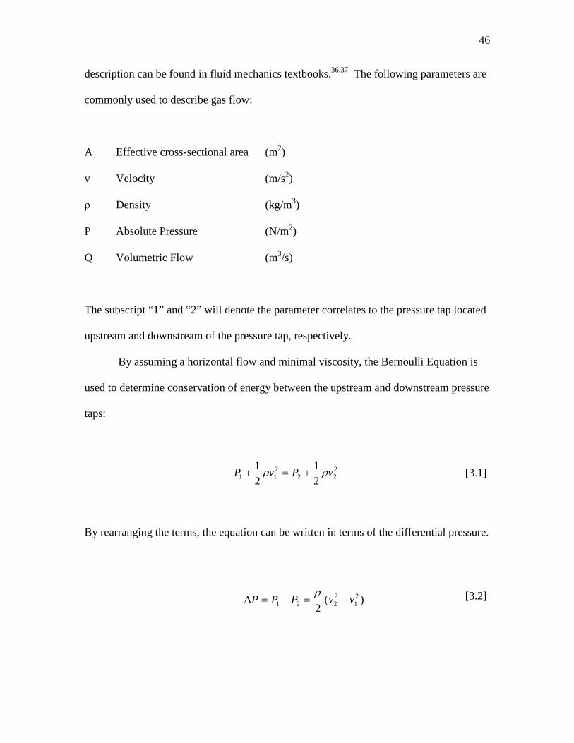
46

description can be found in fluid mechanics textbooks.36,37 The following parameters are

commonly used to describe gas flow:

A Effective cross-sectional area (m2)

v Velocity (m/s2)

ρ Density (kg/m3)

P Absolute Pressure (N/m2)

Q Volumetric Flow (m3/s)

The subscript “1” and “2” will denote the parameter correlates to the pressure tap located

upstream and downstream of the pressure tap, respectively.

By assuming a horizontal flow and minimal viscosity, the Bernoulli Equation is

used to determine conservation of energy between the upstream and downstream pressure

taps:

222

211 2

1

2

1vPvP ρρ +=+ [3.1]

By rearranging the terms, the equation can be written in terms of the differential pressure.

[3.2]

)(2

21

2221 vvPPP −=−=∆

ρ

47

Assuming constant density, the relationship between volumetric flow, area, and

velocity is given by the Equation of Continuity.

2211 vAvAQ == [3.3]

Solving Equation 3.3 for v1 and substituting it into Equation 3.2 yields:

( ) 2

2

2

1

2

1

2222

2 122

vA

A

A

vAvP

−=

−=∆

ρρ [3.4]

where ∆P is the measured differential pressure.

To solve for the volumetric flow, Equation 3.4 is written in terms of v2 and the

equation becomes

ρρ

P

AA

AA

A

A

PAvAQ i

∆

−=

−

∆==

22

21

22

21

21

22

222 2

1

2 [3.5]

where Qi is the ideal flow. To reduce the number of terms in the equation, a constant of

proportionality introduced

ρP

KQi

∆= [3.6]

48

where K has units of square meters.

3.2.2.1. Introduction of temperature and pressure terms. The properties of a

particular gas are dependent on the pressure, volume, and temperature, ideally given by

the equation

nZRTPV = [3.7] where P is the absolute pressure (N/m2), V is the volume (m3), T is the temperature in

Kelvin (K) n is the amount of the gas (mol), Z is a dimensionless compressibility factor,

and R is the universal gas constant (N m/mol K).

The number of moles in a gas can be expressed in terms of the molar mass and the

mass

mM

mn = [3.8]

where m is the mass in kg and Mm is the molar mass in kg/mol.

The density of a fixed volume of gas with a known mass is given by Equation

3.9. The ideal gas law can then be used to introduce the temperature and pressure terms

by

ZRT

PM

V

m m==ρ [3.9]

49

The volumetric flow equation, with the added pressure and temperature terms

from Equation 3.9, then becomes

PM

PZRTKQ

m

∆= [3.10]

3.2.2.2. Correcting to base conditions. In order to correct the measured flow to

standard conditions a method for utilizing the ideal gas law was developed. Briefly

stpstp

stpstp

TZ

VPnR = [3.11]

ff

ff

TZ

VPnR = [3.12]

where the subscript “stp” is used to designate standard temperature and pressure

conditions and “f” refers to the measured conditions of the flowing gas. By setting the

equations equal to each other and differentiating both sides with respect to time, the

volume term becomes volumetric flow so that

ff

ff

stpstp

ststp

TZ

QP

TZ

QP= [3.13]

50

where Qstp and Qf are the volumetric flow rates of the gas relative to the standard

temperature and pressure at sea level and the conditions where the flowing gas was

measured , respectively. Solving Equation 1.13 for Qstp gives

fffstp

stpstpfstp Q

ZTP

ZTPQ = [3.14]

To convert Equation 3.10 from the flowing conditions to standard conditions it is

combined with Equation 3.14

fm

ff

ffstp

stpstpfstp PM

RTPZK

ZTP

ZTPQ

∆= [3.15]

K will absorbs the constant terms as before so that

RZAA

AA

Z

ZK f

f

stp

−= 2

221

22

212 [3.16]

The units of K now become

5

Kmol

mNunitsK

⋅⋅

=⋅ [3.17]

51

And the final equation to convert the volumetric flow Qf to standard conditions Qstp is

given by

fm

f

fstp

stpfstp PM

PTK

TP

TPQ

∆= [3.18]

where the units cancel

2

66

2

53

s

m

skg

mkg

Pamol

kgKPa

Kmol

mN

KPa

KPa

s

m=

⋅⋅

=⋅

⋅⋅

⋅⋅

⋅⋅

= [3.19]

such that the units of flow is given in m3/s.

3.2.2.3. Determining discharge coefficient. A main assumption of the Bernoulli

equation is that no head loss occurs between points (1) and (2), as shown in Figure 3.2.

Therefore, it is necessary to include an empirical coefficient to correct for the difference

between the actual flow rate and the ideal flow rate. Introducing the constant is

advantageous because it allows for the correction of errors that may arise due to changes

in gas velocity composition. The constant, when indexed by the Reynolds number, can

also be used to correct for variations in dynamic viscosity. This constant, known as a

discharge coefficient Cd, is a function of the orifice opening.

Ideally, the flow through the orifice would be given by the equation

iii AQ υ= [3.20]

52

where Qi is the ideal volumetric flow, Ai is the ideal area which is equivalent to the

orifice opening Ao, and vi is the ideal gas flow. Ideal velocity is computed by the

Bernoulli equation.

However, the flow of gas through an orifice is such that the minimum cross-

sectional area of the jet A2 is always smaller than that of the orifice A0. The velocity

profile through the orifice is not uniform, which leads to a point at A2 known as the vena

contracta. At this point the velocity is at its highest due to converging streamlines. Due

to the complex flow profile, it is difficult to measure the value of A2 at the vena

contracta. Head losses associated with turbulent flow caused by the orifice plate also

make it impossible to calculate true flow theoretically. The discharge coefficient relates

the actual flow to the ideal flow:

IdealFlow

ActualFlowCd = [3.21]

so that

id QCQ = [3.22] By this definition the discharge coefficient is an integer that 0 to 1.

The flow discharge is highly dependent on orifice geometry and the Reynolds

number. The Reynolds number, a unit-less dimension used to characterize laminar or

turbulent conditions, is given by

53

µρυD

=Re [3.23]

where ν velocity (m/s)

µ dynamic viscosity (Pa s or N s/m2)

ρ density (kg/m3)

D diameter of Pipe (m)

Using the relationship established in Equation 3.9 for density, the Reynolds

number becomes

f

fm

ZRT

PDM

µ

υ=Re [3.24]

where Mm is the molecular mass, Pf and Tf refer to the pressure and temperature of the

flowing gas, Z is the gas compressibility factor, and R is the universal gas constant.

Equation 3.24 is simplified by combining the constant terms into a constant called “A”

as shown

ZR

DA = [3.25]

54

To a first approximation, the velocity term is proportional to the square-root of the

differential pressure so the Reynolds numbers becomes

f

fm

T

PMPA

µ∆=Re [3.26]

For the purpose of this study, the discharge coefficient will be determined

experimentally and implemented into the final equation of volumetric flow as a lookup

table, which will use the Reynolds number as an index number. When the discharge

coefficient was determined experimentally is it combined with the other constant terms in

Equation 3.18, to give flow coefficient, C. Consequently the coefficient can be greater

than one. A weighted average linear interpolation should be applied to determine values

not specified in the index table.

3.3. Results

3.3.1. Discharge Coefficient

The analogue-to-digital (ADC) differential pressure signal was recorded was

recorded at incremental flow rates from 0 to 300 liters/minute, the maximum flow that

could be obtained with the ventilator. For discharge coefficient analysis the ADC signal

was converted into SI units of pressure. Pressure and temperature of the flowing gas

were measured at 84.5 kPa and 297.5 K, respectively. The molecular mass of air was

defined as 0.028669 kg/mol. According to the National Institute of Standards

Technology, a standard pressure of Pstp = 101.325 kPa and temperature of Tstp = 293.15 K

were used in the calculations.

55

Due to the experimental design, the discharge coefficient was combined with the

constant of proportionality term given in Equation 3.6. For convenience, this term will

be referred to as the flow discharge coefficient, C. Rearranging the terms of Equation

3.18, the discharge coefficient at a given flow becomes

stp

fm

f

fstp

stpf

Q

PM

PT

TP

TP

C

∆

= [3.27]

Because coefficient C takes into account factors including the cross-sectional area and

fluid viscosity, it will not be an integer from 0 to 1.

To create a flow coefficient lookup table, the flow coefficient was indexed by the

Reynolds number. The Reynolds number given in Equation 3.26 includes a constant

term, A, which includes the diameter, gas compressibility factor, and universal gas

constant. The nature of the prototype was such that a specific diameter of the breathing

circuit was not defined. Instead, the constant was set equal to one. The Reynolds

number reported is therefore scaled. This shall be denoted by the prime symbol

following the Reynolds number, R’.

The flow coefficient as indexed by a scaled Reynolds number is given in Figure

3.3. During laminar flow (low Reynolds numbers) there is a sharp spike seen in the flow

coefficient. As the Reynolds number increases the flow coefficient stabilizes around

30.5.

For the index table that would be incorporated into the flow algorithms the flow

coefficient values were weighted. The measured volumetric flow was more dependent on

56

the flow coefficient at low Reynolds numbers than at high ones. For an R’ < 2,300,000,

an average of ±1 data point to the right and the left of the flow coefficient was taken, for

a total of n = 3 data points. Above R’ >= 2,300,000 the flow coefficient remained stable

and was set at a constant value of 30.4822.

The index table is given in Table 3.1. Figure 3.4 is a graphical representation of

the weighted flow coefficients. For values not specified on the table, a linear

interpolation between the two nearest integers should be applied. For example, if an

index of 1,500,000 was returned, the flow coefficient would be a weight average of the

index points of 1,438,328 and 1,559,968.

To test the accuracy of the sensor using the modified discharge coefficient, the

calculated volumetric flow was compared to the recorded volumetric flow. For an

R>=650,000 to be within 3%; for R<650,000 the sensor was accurate to within ±0.8 liter.

3.4. Discussion

The purpose of this effort was to calibrate the prototype flow sensor by

determining the discharge coefficient. Orifice plates are commonly used to measure the

flow of natural gases. The need for a discharge coefficient to account for head losses and

changes in area that cannot be calculated theoretically has been recognized. When the

orifice opening is circular, guidelines set forth by the International Organization of

Standards (ISO) detail the process for determining the discharge coefficient based on

empirical equations (ISO 5167-1).38,39

Ideally, the flow rate could also be calculated experimentally using Equation

3.20, but because the original sensor was designed for exercise applications the orifice

57

opening is not a perfect circle. Instead it includes conduit for saliva and moisture, Figure

3.5, which accumulates when breathing through a mask. Moisture buildup along the

inner wall of the sensor around the orifice ring can effectively change the sensor

geometry. So, while it is necessary to prevent the buildup of fluids within the sensor

housing, it makes the area of the actual orifice opening difficult to calculate theoretically.

The Reynolds number is a dimensional number that is used as a way to quantify

the effects of the inertial and viscous forces within a fluid. When the viscosity forces are

predominant the fluids profiles is streamline. This is known as laminar flow and is

characterized by a constant fluid motion, minimal disruptions, and a Reynolds number

less than 2,300. When the Reynolds number is above 2,300 the flow is turbulent. The

inertial forces become more prevalent and the flow experiences random eddies and other

disturbances. Because the Reynolds number in this study was scaled, the transition from

laminar to turbulent flow does not occur at R=2,300.

The flow coefficient for the prototype sensor revealed a sharp spike at low flows,

followed by a transition period, and then the flow coefficient stabilized. This pattern was

observed in several independent trials. In their studies of small sharp-edged cylindrical

orifices, Ramamurthi et al (1999) found that at low Reynolds numbers the flow profile

varied based on the aspect ratio of the length to the diameter of the orifice (l/d). They

suspect the spike in discharge coefficient could be a result of added pressure due to the

surface tension of water. When the Reynolds number is high, the surface tension induced

pressures are negligible. The discharge coefficient is no longer dependent on the flow

profile (i.e., Reynolds number).40-42

58

As seen in the derivation, the flow coefficient is highly sensitive to changes in the

geometry of the orifice and flow profiles. One limitation of this study was the flow

sensor calibration was based on a single prototype system. Before the system could be

sold commercially several prototype systems with the exact same specifications would be

manufactured. Each individual system could be calibrated. To improve the accuracy of

the flow coefficient, each individual system could be calibrated and the results reported

as a composite flow coefficient table.

Another limitation of the experimental design was the sensor was tested under

constant airflow. During a practical application, the sensor will be subjected to various

expired flow rates as the individual breaths in and out. At low flows the resolution of the

signal decreases, but at high flows the signal strength is high. During a normal breath

this could be problematic since the flow during the exhale breath is drawn out. However,

during exercise the transition of flow from an inhale to and exhale happens rapidly and

there is a minimal amount of time spent while flow is low.

59

Figure 3.1 Experimental setup for flow calibration

ESPRIT Ventilator

VT Plus

Sensor

FloTrac Elite

Laptop

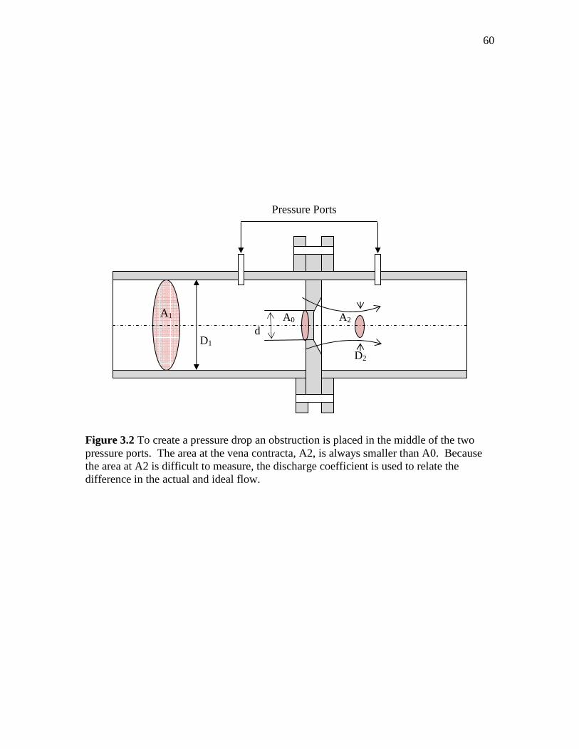
60

Figure 3.2 To create a pressure drop an obstruction is placed in the middle of the two pressure ports. The area at the vena contracta, A2, is always smaller than A0. Because the area at A2 is difficult to measure, the discharge coefficient is used to relate the difference in the actual and ideal flow.

A1 A0 A2

D1 d

D2

Pressure Ports

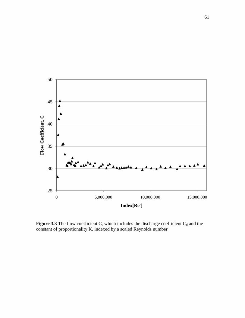
61

Figure 3.3 The flow coefficient C, which includes the discharge coefficient Cd and the constant of proportionality K, indexed by a scaled Reynolds number

25

30

35

40

45

50

0 5,000,000 10,000,000 15,000,000

Flo

w C

oeffi

cien

t, C

Index[Re']

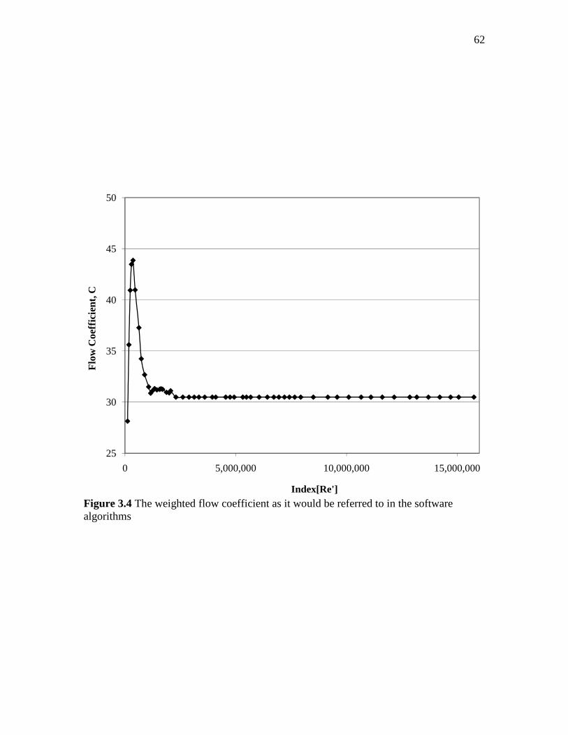
62

Figure 3.4 The weighted flow coefficient as it would be referred to in the software algorithms

25

30

35

40

45

50

0 5,000,000 10,000,000 15,000,000

Flo

w C

oeff

icie

nt, C

Index[Re']

63

Figure 3.5 End view of the differential pressure orifice opening.

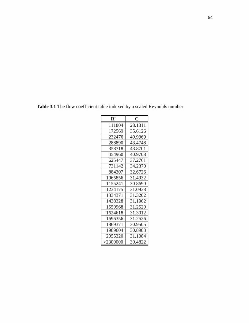
64

Table 3.1 The flow coefficient table indexed by a scaled Reynolds number

R' C 111804 28.1311 172569 35.6126 232476 40.9369 288890 43.4748 358718 43.8701 454960 40.9708 625447 37.2761 731142 34.2370 884307 32.6726

1065856 31.4932 1155241 30.8690 1234175 31.0938 1334371 31.3202 1438328 31.1962 1559968 31.2520 1624618 31.3012 1696356 31.2526 1869371 30.9505 1989604 30.8983 2055320 31.1084

>2300000 30.4822

65

CHAPTER 4

4. VALIDATION OF LUMINESCENCE QUENCHING OXYGEN SENSOR

VALIDATION OF LUMINESCENCE QUENCHING OXYGEN SENSOR

4.1. Introduction

In vitro testing of oxygen uptake during exercise was performed using a propane

combustion patient lung simulator. The ratio of the rate of carbon dioxide production per

minute (VCO2) over the rate of oxygen consumption per minute (VO2) is known as the

respiratory quotient (RQ). When burned completely, the combustion of propane to form

carbon dioxide and water vapor has a standard RQ of 0.6. This method is often used to

check the accuracy of VO2 and VCO2 measurements for metabolic monitors.43,44

In previous bench testing of the oxygen uptake measurements for clinical use, the

oxygen sensor was found to be accurate to within 0.3±2.8% of the measured oxygen.

When compared with the clinical gold standard device (Deltatrac, Datex, Helsinki,

Finland) the error in the oxygen consumption of 2.2±4.1% was found to be well within an

acceptable range for clinical use. The system was again tested on 14 intensive care unit

patients and found to be within 1.7±6.9% of the reference analyzer.

Oxygen consumption will be determined theoretically and then compared to the

measurements recorded during the propane simulation with constant air flow. To be

suitable for an exercise application, the oxygen sensor measurement should be accurate to

within ±5% of the measured fraction of expired oxygen.

66

4.2. Materials and Methods

4.2.1. Experimental Design

The propane lung simulator setup is shown in Figure 4.1. A propane burner was

mounted inside a glass chamber with inlet and outlet flows. The inlet flow was

connected to an ESRIT Ventilator (Phillips-Respironics, Carlsbad, California), which

provided the oxygen necessary for combustion. The rate of inspired air VI (L/min) was

measured using the VT Plus Gas Flow Analyzer (Bio-Tek, Winooski, Vermont) before it

entered the chamber. The differential pressure and oxygen sensors provided on-airway

analysis of the gas as it exited the chamber in the outlet flow.

The burner was connected to a flow rotometer with a needle valve (NV). The

arbitrary settings on the needle valve controlled the propane flow rate. To keep the

system cool and prevent damage to the parts, cold water was circulated in coils within the

glass chamber.

The oxygen and differential pressure sensors were connected to a FloTrac Elite

(Phillips-Respironics, Carlsbad, California), which used algorithms to determine the

fraction of expired oxygen and gas flow. The FloTrac Elite was connected to a laptop,

which recorded the various parameters including fraction of expired carbon dioxide

(FeCO2), the fraction of expired oxygen (FeO2), and flow signals.

4.2.2. Calibration Curve

It was first necessary to create a calibration curve relating the amount of propane

burned (i.e., the NV placement on the flow rotometer) with the oxygen consumed. The

propane tank was placed on a scale and the mass in grams was recorded. A scale

67

recorded the mass of propane burned at four settings (15, 20, 25, and 30) on the needle

valve. The propane NV was held constant while the air flow from the ventilator was

varied. Air flows of approximately 10, 15, 25, 40, and 60 L/min were selected. At each

setting measurements were taken every 3 minutes for 9 minutes. The rate of propane

consumption was dependent on the NV placement and did not vary across the air flow

rates. The average propane mass loss for 45 minutes was reported in the calibration

curve.

When oxygen is not a limiting factor, the molecular formula for complete propane

combustion is given by

C3H8 (propane) + 5 O2 → 3 CO2 + 4 H2O + heat [4.1]

The amount of propane consumed in grams/min was converted to mol/min using

the molecular weight of propane. Five moles of oxygen are consumed for every one

mole of propane. The ideal gas law was used to determine the number of ml/min of O2

consumed at ambient conditions. At standard conditions one mole of gas occupies 22.4

liters.

4.2.3. Validation of O2 Sensor During Simulated Exercise

The accuracy of the oxygen sensor was tested at four propane combustions levels,

which corresponded to the needle valve placement at 15, 20, 25 and 30. At ambient

conditions, the VO2 at these levels was determined in the calibration to be approximately

323, 430, 538, and 646 ml/min, respectively.

68

The same NV and flow rate settings were used for the O2 sensor validation as in

the calibration curve. A stabilization period of 5 minutes was allowed in between each

NV setting. Then the VI, FeO2, FeCO2, and differential pressure were all recorded every 3

minutes for 9 minutes total at each flow increment and the average was reported.

Relative humidity and temperature of the inspired and expired gas were monitored using

an Omega RH81 Thermo Hydrometer (Omega, Stamford, Connecticut).

4.2.4. Relative Humidity Correction

Dry air is a composite of 78.8% nitrogen, 20.9% oxygen, 0.9% argon, and 0.03%

carbon dioxide. However, for most practical applications there is also 1-3% water vapor

present, so it was necessary to adjust the composition percentages accordingly.

Relative humidity (RH) is the ratio of the actual partial pressure of water vapor in

ambient conditions and the saturation pressure of water at the ambient temperature

sat

v

p

pRH =% [4.2]

where RH is the relative humidity, pv is the partial pressure of water vapor, and psat is the

saturation pressure of water at the ambient temperature. The saturation pressure of water

at a given temperature is derived empirically where

−−

=85.35

65.20485.7exp10*1078.6

T

Tpsat [4.3]

69

where T is the temperature in Kelvin.

Water vapor changes the fraction of inspired gases so that

bar

vI p

pOHF =2 [4.4]

and

2093.0*2bar

vbarI p

ppOF

−= [4.5]

For the purposes of this study the fraction of inspired argon and carbon dioxide are

negligible.

4.2.5. Analysis of Calculated FeO2

The rate of oxygen consumption (VO2) is the difference between the volumes of

inspired air (VI) multiplied by the fraction of inspired oxygen (FIO2) and the volume of

expired air (VE) multiplied by the fraction of expired oxygen (FeO2) as shown

( ) ( )222 ** OFVOFVOV EEII&&& −= [4.6]

N2 is neither used nor produced in metabolism. Therefore, the volume of N2 inhaled

must be equal to the volume exhaled according to the Haldane transformation as follows

70

22 NFVNFV IEII ×=× && [4.7] where

OHFCOFOFNF IIII 2222 1 −−−= [4.8]

OHFCOFOFNF EEEE 2222 1 −−−= [4.9] It follows that by substituting Equations 4.8 and 4.9 into Equation 4.7 and rearranging

the terms the equation becomes

( )( ) I

EEE

III

EN

NI

IE VOHFCOFOF

OHFCOFOF

F

FVV &&&

−−−−−−

==222

222

1

1

2

2 [4.10]

Using this relationship to eliminate VE the theoretical FEO2 at the ambient conditions is

determined by

( ) ( )( ) 2

222

22222 *

1

1* OFV

OHFCOFOF

OHFCOFOFOFVOV EI

EEE

IIIII

&&&

−−−

−−−−= [4.11]

By simplifying the equation and assuming minimal carbon dioxide in the air (i.e. FICO2 =

0) the equation yields

71

( )

( ) 2222

222

2

1

1OF

OHFCOFOF

OHFOFOF

V

OVE

EEE

III

I

−−−

−−−=&

& [4.12]

The known parameters included VI, which was recorded by the VT Plus; VO2; which was

calculated from the calibration curve; and FiO2, FiH20, FeCO2, and FeH20, which were

adjusted based on the relative humidity at ambient conditions. After applying the known

parameters into Equation 4.12, it was a straightforward process to isolate and solve for

the calculated value of FeO2.

4.3. Results

4.3.1. Calibration Curve

The results of the calibration curve are shown in Table 4.1. The total mass loss

from the propane combustion at each needle valve setting is shown in the first column.

The molecular weight of propane was used to calculate the number of moles burned.

Using the ambient conditions and the ideal gas law, the volume in ml/min of oxygen at

each needle valve setting was determined in column four. At standard conditions one

mole of gas occupies 22.4 liters, as shown in the last column. At ambient conditions, the

volume of oxygen consumed (ml/min) was equivalent to 21.544 (R2=0.9998) times the

needle valve placement, Figure 4.2.

4.3.2. Recorded Parameters

At the ambient conditions measured in the lab, the temperature and relative

humidity of the inspired air were T = 304.5 K and a RH = 23.1%. The barometric

pressure was recorded at Pbar = 635 mm Hg. When adjusted for the relative humidity, the

72

fractions of inspired air are as follows FiO2 = 0.206602, FiCO2 = 0, and FiH2O =

0.012891.

The results of the propane combustion simulation are given in Table 4.2. Two

data points are marked with an asterisk. At 10 L/min and a NV = 30 the flame would not

stay lit and no measured parameters were reported. This was most likely caused by the

large propane consumption being limited by available oxygen in the low flow. At 60

L/min and a NV = 15 the VI is lower than at the other flows (~50 L/min instead of ~60

L/min). Although the FiO2 and percent error are reported for this value, it is important to

take the decrease in VI into consideration.

4.3.3. Oxygen Validation Measurements and Percent Error

The recorded FeO2 by the oxygen sensor is given in Table 4.3. From the

calibration curve, the VO2 at each needle valve setting (which relates to the flow of

propane controlled by the rotometer) was determined. Going down the columns for a

given flow rate, the FeO2 measured in the output flow decreased with increasing propane

combustion rates (higher NV settings) and VO2. Moving across the rows, when the

propane combustion is held constant the FeO2 increases with increasing flow rates. The

difference in FeO2 between the NV settings is more pronounced at lower flows. As the

flow increases the difference becomes less significant, Figure 4.3.

The calculated FeO2 was the method described in Section 4.2.5. A comparison of

the calculated FeO2 and the FeO2 recorded by the oxygen sensor is given in Table 4.4.

The percent of error is greatest at the low flows and decreases as the flow increases for a

given propane level. At constant flow the percent error increases as the propane

73

consumed also increases. As previously noted, the flow at NV = 15 and 60 L/min was

lower than the others. While the exact FeO2 could not be measured, the trend remained

consistent.

The chamber design required cooling coils to remove heat within the chamber.

Circulating water was pumped the water through the coils. Ice was occasionally added to

the water to keep the water at 29° C. This had the immediate effect of reducing the

relative humidity in the expired gas, and could possibly why the percent error at NV = 20

and 25 L/min (Table4. 4) was slightly lower than expected even though the recorded

FeO2 (Table 4.3) at that point was within the expected range.

4.4. Discussion

The in vitro simulation of an exercising individual conducted in a propane burn

combustion chamber found the luminescence quenching oxygen sensor to be accurate

within ±6% of the expected FeO2 at the ambient conditions across the entire range of

flows tested. The accuracy of the sensor improved as the flow rates increased.

The experimental design had a few limitations. First, the simulation of exercise

was limited by the size of propane combustion chamber. Flows larger than 60 L/min

would extinguish the flame. During maximal exercise, the minute ventilation of an

average 40 year old male is about 90 L/min. Athletes at their peak have minute

ventilations that can exceed 200 L/min. This chamber size is more representative of the

minute volumes a child would require during exercise.

Another limitation related to the chamber size was the allowable flame size for

the propane combustion. During exercise, a 40 year old male weighing 75 kg may have a

74

VO2 max of 40 ml/kg/min or 3000 ml/min. The flame size limited the maximum oxygen

consumption to about 640 ml/min. So even though the sensor is accurate to within ±3%

at the highest flow rate and VO2 consumption level tested, the accuracy of the oxygen

sensor at higher VO2 levels and flow rates could not be determined.

Relative humidity can also cause errors in the reported oxygen consumption.

Relative humidity of the expired gas was measured and the gas analysis was adjusted

accordingly. At low air flow rates the expired gas was nearly 100% saturated. However,

as the flow rate increased the water concentration in the expired air was diluted. The

relative humidity at 60 L/min was around 25%. Air exhaled from the lungs becomes

saturated, so this limitation in the experimental design must also be considered.

The most significant limitation is most likely caused by a span error due to the

calibration of the oxygen sensor performed by the black box. Span is the variation from

the input oxygen and the output oxygen signal. The oxygen sensor is calibrated by

zeroing the sensor in room air. As shown in Figure 4.3, the expired oxygen signals that

were closest to the inspired oxygen signals had lower error than expired oxygen that was

farther away from the original value. To reduce the span error the sensor should be

zeroed in an additional gas like nitrogen.

Although there were limitations, the purpose of these experiments was to

determine if the luminescence-quenching oxygen sensor designed for low flow

applications could be expanded to include elevated volumetric air flows. During exercise

both flow rates and oxygen consumption levels increase, so it is reasonable to conclude

that the FeO2 measured would still be within the limits of sensitivity for the oxygen

sensor.

75

~ ~ 0 01- ". 0 "- ~ 1- ;.;:: = £~ J ~

e /v;

~J ~

v~ • ,

0 ~ ., ~ "

L

• ~ >

" ~ .; ~~

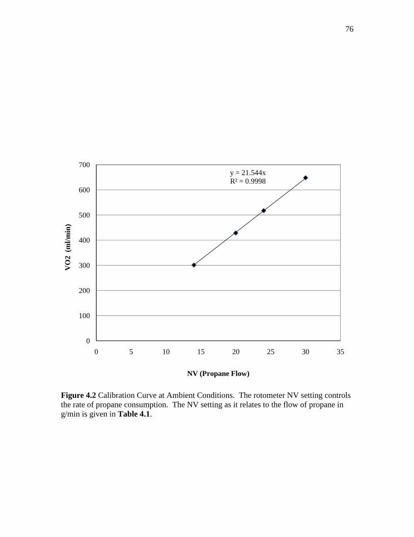
76

Figure 4.2 Calibration Curve at Ambient Conditions. The rotometer NV setting controls the rate of propane consumption. The NV setting as it relates to the flow of propane in g/min is given in Table 4.1.

y = 21.544xR² = 0.9998

0

100

200

300

400

500

600

700

0 5 10 15 20 25 30 35

VO

2 (

ml/m

in)

NV (Propane Flow)

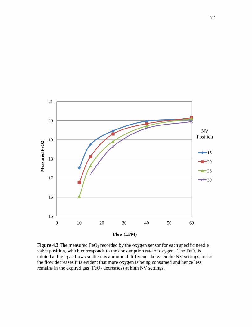
77

Figure 4.3 The measured FeO2 recorded by the oxygen sensor for each specific needle valve position, which corresponds to the consumption rate of oxygen. The FeO2 is diluted at high gas flows so there is a minimal difference between the NV settings, but as the flow decreases it is evident that more oxygen is being consumed and hence less remains in the expired gas (FeO2 decreases) at high NV settings.

15

16

17

18

19

20

21

0 10 20 30 40 50 60

Mea

sure

d F

eO2

Flow (LPM)

15

20

25

30

NV Position

78

Table 4.2 Average (n=3) of VI, FeO2, FeCO2, and FeH20 for the specified NV and flow rate

10 L/min 15 L/min

NV Flow,

VI FeO2 FeCO2 FeH20 NV Flow,

VI FeO2 FeCO2 FeH20

15 9.96 0.1753 0.0207 0.0320 15 15.03 0.1857 0.0140 0.0255 20 10.20 0.1677 0.0276 0.0346 20 15.20 0.1812 0.0186 0.0276 25 9.88 0.1603 0.0322 0.0385 25 15.07 0.1765 0.0227 0.0275

30* 30 15.17 0.1721 0.0260 0.0314

25 L/min 40 L/min

NV Flow,

VI FeO2 FeCO2 FeH20 NV Flow,

VI FeO2 FeCO2 FeH20

15 24.93 0.1946 0.0089 0.0204 15 40.23 0.1998 0.0057 0.0153 20 24.93 0.1903 0.0118 0.0223 20 40.13 0.1984 0.0075 0.0185 25 24.77 0.1891 0.0127 0.0232 25 40.00 0.1973 0.0082 0.0185 30 25.03 0.1865 0.0168 0.0278 30 40.57 0.1960 0.0109 0.0227

60 L/min

NV Flow,

VI FeO2 FeCO2 FeH20

15 48.37** 0.2007 0.0048 0.0134 20 57.93 0.2015 0.0055 0.0152 25 57.23 0.2011 0.0066 0.0163 30 56.90 0.1995 0.0082 0.0198

* Flame would not stay lit at this flow ** Flow did not reach 60 L/min

Table 4.1 Calibration Curve Conversion C3H8 C3H8 5 VO2 VO2 VO2 STP NV g/min mol/min mol/min ml/min ml/min

15 0.095192 0.002159 0.010793 323.1674 241.7565 20 0.126922 0.002878 0.01439 430.8899 322.342 25 0.158653 0.003598 0.017988 538.6123 402.9274 30 0.190383 0.004317 0.021585 646.3348 483.5129

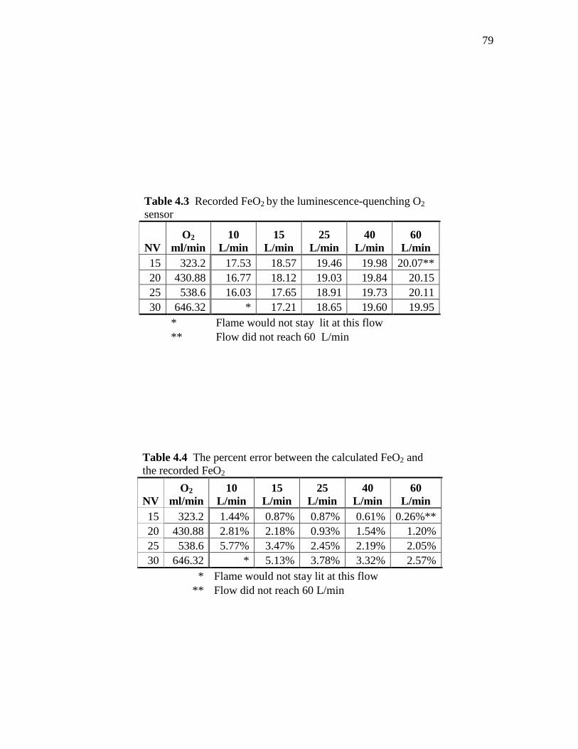
79

Table 4.3 Recorded FeO2 by the luminescence-quenching O2 sensor

NV O2

ml/min 10

L/min 15

L/min 25

L/min 40

L/min 60

L/min 15 323.2 17.53 18.57 19.46 19.98 20.07** 20 430.88 16.77 18.12 19.03 19.84 20.15 25 538.6 16.03 17.65 18.91 19.73 20.11 30 646.32 * 17.21 18.65 19.60 19.95

* Flame would not stay lit at this flow ** Flow did not reach 60 L/min

Table 4.4 The percent error between the calculated FeO2 and the recorded FeO2

NV O2

ml/min 10

L/min 15

L/min 25

L/min 40

L/min 60

L/min 15 323.2 1.44% 0.87% 0.87% 0.61% 0.26%** 20 430.88 2.81% 2.18% 0.93% 1.54% 1.20% 25 538.6 5.77% 3.47% 2.45% 2.19% 2.05% 30 646.32 * 5.13% 3.78% 3.32% 2.57%

* Flame would not stay lit at this flow ** Flow did not reach 60 L/min

80

CHAPTER 5

5. CONCLUSIONS

CONCLUSIONS

5.1. Summary of Results

Although there were many limitations of this study, the overall goal was to

determine if modifying an existing metabolic system for exercise testing was reasonable.

Based on the results presented in this thesis it was concluded that the performance of the

prototype system indicates it would indeed be very possible to build such a system. The

system applications extend to several large markets and would be profitable. A brief

summary of the conclusions for each specific aim presented in this thesis is presented in

the following sections. Future work and a few possible applications for luminescence-

quenching technology in portable metabolic gas analysis systems is also provided.

5.1.1. Prototype Design and Flow Diversion Analysis

The first aim of this study was to build a prototype system with a breathing circuit

capable of monitoring exhaled gases flows and concentration during exercise. Flow

sensor housing was obtained from a commercially available unit. The gas sensor was

inserted into the main lumen of the flow housing at a 90o angle creating a T- piece. It was

hoped that some air would be diverted from the main flow across the sensor for gas

analysis. However, the input coupling of the gas analysis sensor was significantly

81

narrower than the flow housing exit orifice. The resistance created by the narrowing of

the input coupling was too great, and the flow exited through the main flow orifice. To

guide flow to the sensor, the extension of the input coupling into the main flow was

lengthen and a portion of the input coupling diameter was removed. This acted as a

conduit and flow was then diverted to the sensor. The resistance was further minimized

when the sensor was inserted at a 45o angle into the main lumen.

Through testing of the end-tidal CO2 with this geometry and a reference site, this

configuration was selected. The circuit design requires a tradeoff between the resistance

to breathing and strength of the differential pressure drop signal. A differential pressure

signal of at around 10 cm H2O at 300 L/min was obtained. The resistance to flow

calculated at 400 L/min was around 3.14 cm H2O/L/s for the modified breathing circuit.

The resistance was slightly higher than the baseline, a standard differential pressure

casing, which had an estimated resistance of 2.81 cm H2O/L/s at the same flow. The

prototype system demonstrated strong signal strength at high flows, which was desirable.

However, the resistance to flow calculated at high flows was slightly above the

recommended values.

So, while modifying the existing breathing circuit allowed for more air flow and

improved the signal strength by creating a larger differential pressure drop, it adversely

affected the back pressure resistance that a user would experience which could lead to

premature gas analysis results. Based on the results, it is reasonable to conclude that

with a few more slight modifications the current breathing circuit could be used for

exercise stress testing. However, more work is needed to optimize the breathing circuit

design.

82

5.1.2. Flow Sensor Calibration - Discharge Coefficient Table

Flow profiles are subject to specific geometries, therefore, the second aim of this

study was to calibrate the flow using the existing sensor configuration. Nonlinear

differential pressure flow sensors calculate flow as roughly proportional to the square

root of the differential pressure drop. It was necessary to introduce a correction flow

coefficient because head losses in the actual flow result in slightly different flow rates

than the calculated value. This was achieved by calculating the predicted flow through

the orifice and comparing it with the actual measured flow to equate a flow coefficient

correction factor that was dependent on the Reynolds number of the flow. With the flow

coefficient correction factor, the flow reported by the sensor was accurate to within ±3%

or ±1 L. The accuracy of the flow improved with an increasing Reynolds number.

5.1.3. Oxygen Sensor Calibration

The final aim of this research was to calibrate the luminescence quenching

oxygen sensor using a propane combustion patient simulator. The oxygen consumption

for the complete combustion of propane was calculated theoretically. Then, using the

propane simulator which burns propane at a defined rate, the oxygen in the expired gas

flow was also measured and used to determine the exact amount of oxygen consumed.

The accuracy of the luminescence quenching oxygen sensor was found to be within ±6 %

of the measured FeO2 when compared with the theoretical oxygen consumption.

At low levels of propane combustion and air flow the reported accuracy of the

oxygen sensor was similar to previous trials. For a given flow the accuracy of the sensor

decreased as the oxygen consumption increased, indicating that the flame size was a

83

limiting factor. The accuracy across the flow range for a given level of oxygen

consumption also improved with increasing flow rates. The sensor was most accurate

when there was a minimal difference between the fraction of expired oxygen and the

concentration of oxygen present for the initial calibration of the system, indicating a span

error.

5.2. Future Work

The work presented in this thesis was meant to be the first phase in determining

the plausibility of constructing a prototype breathing circuit for high flow applications

from an existing system used for gas analysis and indirect calorimetry purposes. Before

the system could be recommended as an exercise stress analysis instrument, several more

phases of research would need to be conducted.

Future work would include building several more prototype breathing circuits.

The resistance experienced by the user could be further minimized to fall within the ATS

standard for a monitoring device. Although discharge coefficient seems to stabilize at

higher flows, the flow could be characterized to ± 400 L/min. Bench testing of the

oxygen sensor using a larger propane combustion chamber could model more realistic

oxygen consumption levels in an exercising adult. For VO2 max consumption, the levels

can reach around 6000 mL/min – well past the scope of the 650 mL/min used for this

study.

Another phase of research could include testing other parameters including VCO2

max and sensor performance using a patient lung simulator instead of constant air flow.

84

The final phase of research would include constructing the actual breathing mask with

intake valves. The system then needs to be validated using human volunteers.

5.3. Possible Applications

There is currently a strong market for portable metabolic analysis systems. The

prototype system is one of the smallest available. It is less than 5 in3 and weighs less than

0.5 Kg total. Moreover, it requires minimal power to operate, is self-calibrating, and user

friendly. Given in this section are some possible applications for such a system.

5.3.1. Portable Exercise Testing

Portable metabolic monitors are a growing trend in the field of exercise and sports

medicine. Athletes and exercise enthusiasts are interested in portable systems to be worn

during submaximal workouts as the gas analysis information can be used to guide

training programs. Health spas, gyms, personal trainers, and nutritionists advertise gas

analysis as a tool for making healthy lifestyle choices. Through a process known as

indirect calorimetry, gas analysis can be used to determine an individual’s resting

metabolic rate (RMR). Because this value accounts for nearly 70% of the individual’s

daily energy expenditure it can be used to guide weight loss programs or for nutritional

programs.

The systems must be simple to use, accurate, self-calibrating, fast, and

affordable.34 There has been some discussion on the validity of these portable devices as

they often report significantly different results than standard metabolic carts.45-48

85

5.3.2. NASA

In space several regulatory mechanisms in the cardiovascular system are adapted

to the microgravity environment. These adaptations adversely results in cardiovascular

deconditioning, bone density loss, and muscular atrophy.49,50 Upon returning to the

Earth’s gravitation field some degree of orthostatic intolerance has been noted in even

short duration flights of only a few hours.51,52 This cardiovascular instability is even

more pronounced during prolonged exposure to microgravity and may only be partially

reversible. As space exploration progresses from short to long term duration (months to

years) flights, it will become more imperative for both the mental and physical well-being

of crew members that effective countermeasures be developed.53-55

The health of astronauts is closely monitored before, during, and after space flight

through periodic noninvasive stress tests.56,57 The most commonly measured parameter,

aboard the space station is maximum oxygen uptake (VO2 max) because multiple body

systems must work together during exercise to facilitate the transport of oxygen to the

tissues and meet the increased energy requirements. Consequently, VO2 max helps track

cardiovascular deconditioning due to weightlessness and assess the effectiveness of

resistive exercises.58,59

NASA currently utilizes a random access mass spectrometer (RAMS) system

known as the Gas Analyzer System for Metabolic Analysis Physiology (GASMAP) to

measure crew aerobic capacity. The GASMAP has the drawback of being of being large

and bulky. It requires one 1 x 8 panel unit drawer and two 1 x 4 panel unit drawers and

weighs 51 kg total. It also requires significant amount of power (205 watts).

86

REFERENCES

1. McClave SA, Lowen CC, Kleber MJ, McConnell JW, Jung LY, Goldsmith LJ:

Clinical use of the respiratory quotient obtained from indirect calorimetry. Journal of Parenteral and Enteral Nutrition 2003; 27: 21-26

2. Wolff HS: Modern techniques for measuring energy expenditure. Proceedings of

the Nutrition Society 1956; 15: 77-80 3. Shephard RJ: A critical examination of the Douglas bag technique. The Journal of

Physiology 1955; 127: 515-524 4. Badman ER, Cooks RG: Special feature: Perspective - Miniature mass analyzers.

Journal of Mass Spectrometry 2000; 35: 659-671 5. El-Aneed A, Cohen A, Banoub J: Mass Spectrometry, Review of the basics:

Electrospray, MALDI, and commonly used mass analyzers. Applied Spectroscopy Reviews 2009; 44: 210-230

6. Palmer PT, Limero TF: Mass spectrometry in the U.S. space program: Past,

present, and future. Journal of the American Society for Mass Spectrometry 2001; 12: 656-675

7. Merilainen PT: Metabolic monitor. International Journal of Clinical Monitoring

and Computing 1987; 4: 167-178 8. Macfarlane DJ: Automated metabolic gas analysis systems - A review. Sports

Medicine 2001; 31: 841-861 9. Hodges LD, Brodie DA, Bromley PD: Validity and reliability of selected

commercially available metabolic analyzer systems. Scandinavian Journal of Medicine & Science in Sports 2005; 15: 271-279

10. Saklad M, Sullivan M, Paliotta J, Lipsky M, Brown BR, Jr.: Pneumotachography:

A new, low-dead-space, humidity-independent device. Anesthesiology 1979; 51: 149-153

87

11. Jaffe MB: Infrared measurement of carbon dioxide in the human breath: "Breathe-through" devices from Tyndall to the present day. Anesthesia & Analgesia 2008; 107: 890-904

12. Clark LCJR, Wolf R, Granger D, Taylor Z: Continuous recording of blood

oxygen tensions by polarography. Journal Applied Physiology 1953; 6: 189-193 13. Kanwisher J: Polarographic oxygen electrode. Limnology and Oceanography

1959; 4: 210-217 14. Stambouli AB, Traversa E: Solid oxide fuel cells (SOFCs): A review of an

environmentally clean and efficient source of energy. Renewable and Sustainable Energy Reviews 2002; 6: 433-455

15. Kovacich RP, Martin NA, Clift MG, Stocks C, Gaskin I, Hobby J: Highly

accurate measurement of oxygen using a paramagnetic gas sensor. Measurement Science and Technology 2006: 1579

16. Schmid U, Seidel H, Mueller G, Becker T: Theoretical considerations on the

design of a miniaturised paramagnetic oxygen sensor. Sensors and Actuators B: Chemical 2006; 116: 213-220

17. Turner PG, Dugdale A, Young IS, Taylor S: Portable mass spectrometry for

measurement of anaesthetic agents and methane in respiratory gases. Veterinary Journal 2008; 177: 36-44

18. Orr J, Brewer, Lara: Oxygen uptake (VO2) measurement system based on novel

luminescence-quenching on-airway oxygen sensor. Anesthesiology 2007; A1642 19. Orr J, Brewer, Lara: Clinical evaluation of an on-airway system to measure

oxygen uptake. Anesthesiology 2008; A281 20. Orr J, Brewer, Lara: Evaluation in volunteers of a VO2 measurement system

based on a novel on-airway oxygen sensor. Anesthesiology 2008; A1689 21. Saltin B: Malleability of the system in overcoming limitations: Functional

elements. Journal Experimental Biology 1985; 115: 345-354 22. Bouchard C, Dionne FT, Simoneau J-A, Boulay MR: 2: Genetics of aerobic and

anaerobic performances. Exercise and Sport Sciences Reviews 1992; 20: 27-58 23. Bouchard C BM, Simoneau JA, Lortie G, Pérusse L.: Heredity and trainability of

aerobic and anaerobic performances. An update. Sports Medicine 1988; 5: 69-73

88

24. Saltin B, Kristina N, Costill DL, Stein E, Eva J, Birgitta E, Gollnick PD: The nature of the training response; peripheral and central adaptations to one-legged exercise. Acta Physiologica Scandinavica 1976; 96: 289-305

25. Gollnick PD, Armstrong RB, Saubert CWt, Piehl K, Saltin B: Enzyme activity

and fiber composition in skeletal muscle of untrained and trained men. Journal Applied Physiology 1972; 33: 312-319

26. Astrand P-OaR, K: The textbook of work physiology: Physiological bases of

exercise 3 edition. New York, McGraw-Hill, 1986 27. Standardization of spirometry, 1994 update. American Thoracic Society.

American Journal Respiratory Critical Care Medicine 1995; 152: 1107-36 28. Ross RM, Beck KC, Casaburi R, Johnson BD, Marciniuk DD, Wagner PD,

Weisman IM: ATS/ACCP statement on cardiopulmonary exercise testing. American Journal Respiratory Critical Care Medicine 2003; 167: 1451-

29. Johnson AT, Scott WH, Lausted CG, Benjamin MB, Coyne KM, Sahota MS,

Johnson MM: Effect of respirator inspiratory resistance level on constant load treadmill work performance. American Industrial Hygiene Association Journal 1999; 60: 474-479

30. Johns DP, Ingram CM, Khov S, Rochford PD, Walters EH: Effect of breathing

circuit resistance on the measurement of ventilatory function. Thorax 1998; 53:: 944-948

31. Coyne K, Caretti D, Scott W, Johnson A, Koh F: Inspiratory flow rates during

hard work when breathing through different respirator inhalation and exhalation resistances. Journal of Occupational and Environmental Hygiene 2006; 3: 490-500

32. Deno NS, Kamon E, Kiser DM: Physiological responses to resistance breathing

during short and prolonged exercise. American Industrial Hygiene Association Journal 1981; 42: 616 - 623

33. Page RT: Constant flow orifice meters of low capacity. Industrial & Engineering

Chemistry Analytical Edition 1935; 7: 355-358 34. Andre D, Wolf, Donna: Recent advances in free-living physical activity

monitoring: A review. Journal Diabetes Scientific Technology 2007; 1: 760-767 35. Keyser D, R., Jeffrey, R. Friedman: Extrapolation and curve-fitting of calibration

data for differential pressure flow meters. Journal of Engineering for Gas Turbines and Power 2010; 132: 024501

89

36. Finnemore EJ, Franzini, Joseph B: Fluid mechanics with engineering applications, 10 edition. Boston, McGraw Hill, 2002

37. Munson BR, Young, Donald F., Okiishi, Theodore H.: Fundamentals of fluid

mechanics, 4 edition. New York, John Wiley & Sons, Inc., 2002 38. Measurement of fluid flow by means of pressure differential devices, Part 1:

Orifice plates, nozzels, and Venturi tubes inserted in circular cross-section conduits running full. International Organization of Standards, 1991

39. Reader-Harris MJ, Sattary JA: The orifice plate discharge coefficient equation.

Flow Measurement and Instrumentation 1990; 1: 67-76 40. Laws EM, Ouazanne AK: Compact installations for differential flowmeters. Flow

Measurement and Instrumentation 1994; 5: 79-85 41. Reed SB, Sprange MP: Flowmeter calibrated for any gas in the range of 1 to 500

liters per hour. Industrial & Engineering Chemistry Fundamentals 1968; 7: 651-655

42. Johansen FC: Flow through pipe orifices at low Reynolds numbers. Proceedings

of the Royal Society of London. Series A, Containing Papers of a Mathematical and Physical Character 1930; 126: 231-245

43. Weissman C, Sardar A, Kemper M: In vitro evaluation of a compact metabolic

measurement instrument. Journal of Parenteral and Enteral Nutrition 1990; 14: 216-221

44. Melendez JA, Veronesi M, Barrera R, Ferri E, Miodownik S: Determination of

metabolic monitor errors and precision under clinical conditions. Clinical Nutrition 2001; 20: 547-551

45. Kretsch MJ, Blanton CA, Baer D, Staples R, Horn WF, Keim NL: Measuring

energy expenditure with simple low cost tools. Journal of the American Dietetic Association 2004; 104: 13

46. Nieman DC, Trone GA, Austin MD: A new handheld device for measuring

resting metabolic rate and oxygen consumption. Journal of the American Dietetic Association 2003; 103: 588-593

47. Kautza BC, Kastello GM, Sothmann MS: Validation of MedGraphics' VO2000

Portable Metabolic Analyzer and a modified pneumotachometer. Medicine & Science in Sports & Exercise 2004; 36: S222

90

48. Yeo S, Ronis DL, Antonakos CL, Speers M, Murphy S, Hayashi R, Stegman N: Evaluation of a portable metabolic system with sedentary pregnant women. Medicine & Science in Sports & Exercise 2003; 35: S193

49. Nicgossian AE, Charles JB, Bungo MW, Leach-Huntoon CS: Cardiovascular

function in space flight. Acta Astronautica 1991; 24: 323-328 50. Aubert AE, Beckers F, Verheyden B: Cardiovascular function and basics of

physiology in microgravity. Acta Cardiologica 2005; 60: 129-151 51. Levy MN TJ: Cardiovascular deconditioning of space flight. Physiologist 1983;

26: 297-303 52. Convertino VA: Status of cardiovascular issues related to space flight:

Implications for future research directions. Respiratory Physiology & Neurobiology 2009; 169: S34-S37

53. Leblanc A, Rowe R, Schneider V, Evans H, Hedrick T: Regional muscle loss

after short duration spaceflight. Aviation Space and Environmental Medicine 1995; 66: 1151-1154

54. West JB: Historical perspectives: Physiology in microgravity. Journal of Applied

Physiology 2000; 89: 379-384 55. Macias BR, Groppo ER, Eastlack RK, Watenpaugh DE, Lee SMC, Schneider

SM, Boda WL, Smith SM, Cutuk A, Pedowitz RA, Meyer RS, Hargens AR: Space exercise and earth benefits. Current Pharmaceutical Biotechnology 2005; 6: 305-317

56. Greenleaf JE, Bulbulian R, Bernauer EM, Haskell WL, Moore T: Exercise-

training protocols for astronauts in microgravity. Journal of Applied Physiology 1989; 67: 2191-2204

57. Levine BD, Lane LD, Gaffney FA, Buckey JC, Blomqvist CG: Maximal exercise

performance after adaptation to microgravity. Medicine and Science in Sports and Exercise 1994; 26: S112

58. Convertino VA: Planning strategies for development of effective exercise and

nutrition countermeasures for long-duration space flight. Nutrition 2002; 18: 880-888

59. Ferretti G, Capelli C: Maximal O-2 consumption: Effects of gravity withdrawal

and resumption. Respiratory Physiology & Neurobiology 2009; 169: S50-S54