fault location algorithms, observability and …

University of Kentucky University of Kentucky

UKnowledge UKnowledge

Theses and Dissertations--Electrical and Computer Engineering Electrical and Computer Engineering

2014

FAULT LOCATION ALGORITHMS, OBSERVABILITY AND FAULT LOCATION ALGORITHMS, OBSERVABILITY AND

OPTIMALITY FOR POWER DISTRIBUTION SYSTEMS OPTIMALITY FOR POWER DISTRIBUTION SYSTEMS

Wanjing Xiu University of Kentucky, [email protected]

Right click to open a feedback form in a new tab to let us know how this document benefits you. Right click to open a feedback form in a new tab to let us know how this document benefits you.

Recommended Citation Recommended Citation Xiu, Wanjing, "FAULT LOCATION ALGORITHMS, OBSERVABILITY AND OPTIMALITY FOR POWER DISTRIBUTION SYSTEMS" (2014). Theses and Dissertations--Electrical and Computer Engineering. 48. https://uknowledge.uky.edu/ece_etds/48

This Doctoral Dissertation is brought to you for free and open access by the Electrical and Computer Engineering at UKnowledge. It has been accepted for inclusion in Theses and Dissertations--Electrical and Computer Engineering by an authorized administrator of UKnowledge. For more information, please contact [email protected].

http://uknowledge.uky.edu/

http://uknowledge.uky.edu/

https://uknowledge.uky.edu/

https://uknowledge.uky.edu/ece_etds

https://uknowledge.uky.edu/ece_etds

https://uknowledge.uky.edu/ece

https://uky.az1.qualtrics.com/jfe/form/SV_9mq8fx2GnONRfz7

mailto:[email protected]

STUDENT AGREEMENT: STUDENT AGREEMENT:

I represent that my thesis or dissertation and abstract are my original work. Proper attribution

has been given to all outside sources. I understand that I am solely responsible for obtaining

any needed copyright permissions. I have obtained needed written permission statement(s)

from the owner(s) of each third-party copyrighted matter to be included in my work, allowing

electronic distribution (if such use is not permitted by the fair use doctrine) which will be

submitted to UKnowledge as Additional File.

I hereby grant to The University of Kentucky and its agents the irrevocable, non-exclusive, and

royalty-free license to archive and make accessible my work in whole or in part in all forms of

media, now or hereafter known. I agree that the document mentioned above may be made

available immediately for worldwide access unless an embargo applies.

I retain all other ownership rights to the copyright of my work. I also retain the right to use in

future works (such as articles or books) all or part of my work. I understand that I am free to

register the copyright to my work.

REVIEW, APPROVAL AND ACCEPTANCE REVIEW, APPROVAL AND ACCEPTANCE

The document mentioned above has been reviewed and accepted by the student’s advisor, on

behalf of the advisory committee, and by the Director of Graduate Studies (DGS), on behalf of

the program; we verify that this is the final, approved version of the student’s thesis including all

changes required by the advisory committee. The undersigned agree to abide by the statements

above.

Wanjing Xiu, Student

Dr. Yuan Liao, Major Professor

Dr. Caicheng Lu, Director of Graduate Studies

FAULT LOCATION ALGORITHMS, OBSERVABILITY AND

OPTIMALITY FOR POWER DISTRIBUTION SYSTEMS

_________________________________________________________________________

DISSERTATION

_________________________________________________________________________

A dissertation submitted in partial fulfillment of the

requirements for the degree of Doctor of Philosophy in the

College of Engineering at the University of Kentucky

By

Wanjing Xiu

Lexington, Kentucky

Director: Dr. Yuan Liao, Associate Professor of Electrical and Computer Engineering

Lexington, Kentucky

2014

Copyright © Wanjing Xiu 2014

ABSTRACT OF DISSERTATION



Power outages usually lead to customer complaints and revenue losses. Consequently,

fast and accurate fault location on electric lines is needed so that repair work can be

carried out as fast as possible.

Chapter 2 describes novel fault location algorithms for radial and non-radial

ungrounded power distribution systems. For both types of systems, fault location

approaches using line to neutral or line to line measurements are presented. It’s assumed

that network structure and parameters are known, so that during-fault bus impedance

matrix of the system can be derived. Functions of bus impedance matrix and available

measurements at substation are formulated, from which the unknown fault location can

be estimated. Evaluation studies on fault location accuracy and robustness of fault

location methods to load variations and measurement errors has been performed.

Most existing fault location methods rely on measurements obtained from meters

installed in power systems. To get the most from a limited number of meters available,

optimal meter placement methods are needed. Chapter 3 presents a novel optimal meter

placement algorithm to keep the system observable in terms of fault location

determination. The observability of a fault location in power systems is defined first.

Then, fault location observability analysis of the whole system is performed to determine

the least number of meters needed and their best locations to achieve fault location

observability. Case studies on fault location observability with limited meters are

presented. Optimal meter deployment results based on the studied system with equal and

varying monitoring cost for meters are displayed.

To enhance fault location accuracy, an optimal fault location estimator for power

distribution systems with distributed generation (DG) is described in Chapter 4. Voltages

and currents at locations with power generation are adopted to give the best estimation of

variables including measurements, fault location and fault resistances. Chi-square test is

employed to detect and identify bad measurement. Evaluation studies are carried out to

validate the effectiveness of optimal fault location estimator. A set of measurements with

one bad measurement is utilized to test if a bad data can be identified successfully by the

presented method.

KEY WORDS: distribution systems, fault location observability, optimal fault location

estimator, optimal meter placement, ungrounded systems.

_______________________

Wanjing Xiu _______________________

July 19, 2014



By

Wanjing Xiu

Dr. Yuan Liao

___________________________

Director of Dissertation

Dr. Caicheng Lu

___________________________

Director of Graduate Studies

July 19, 2014

___________________________

Date

iii

ACKNOWLEDGEMENTS

I would like to express my sincerest gratitude and appreciation to my dissertation advisor,

Dr. Yuan Liao, for his patience and expertise in guiding and helping me overcome every

challenge and make steady progress. This dissertation would be impossible without his

extensive knowledge and innovative ideas in this field.

I would also like to thank Dr. Paul Dolloff, Dr. Yuming Zhang, Dr. Alan Male

and Dr. Zongming Fei, for serving as Doctoral Advisory Committee, and for the

invaluable advices they gave.

Thanks to my labmates, Ning Kang, Yan Du, Jiaxiong Chen, Aleksi and

Xiangqing Jiao, for their endless support.

Last but not least, I would like to extend my deepest gratitude to my parents and

my husband, for their endless love and support.

iv

TABLE OF CONTENTS

ACKNOWLEDGEMENTS ............................................................................................... iii

LIST OF TABLES ............................................................................................................ vii

LIST OF FIGURES ............................................................................................................ x

Chapter 1 Introductions ............................................................................................... 1

1.1 Background .......................................................................................................... 1

1.2 Review of Fault Location Methods for Power Systems ....................................... 2

1.3 Dissertation Outline.............................................................................................. 8

Chapter 2 Fault Location for Ungrounded Radial and Non-radial Distribution

Systems ..................................................................................................................... 10

2.1 Introduction ........................................................................................................ 10

2.1.1 Basic Idea of Proposed Methods................................................................. 10

2.1.2 Notations Used in the Proposed Fault Location Methods .......................... 11

2.1.3 Construction of Bus Impedance Matrix ...................................................... 13

2.2 Fault Location Methods for Ungrounded Radial Distribution Systems Using

Line to Neutral Voltages and Line Currents ................................................................. 14

2.2.1 LL Faults ..................................................................................................... 16

2.2.2 LLL Faults .................................................................................................. 17

2.3 Fault Location Methods for Ungrounded Radial Distribution Systems Using

Line to Line Voltages and Line Currents ...................................................................... 20

v

2.3.1 LL Faults ..................................................................................................... 20

2.3.2 LLL Faults .................................................................................................. 21

2.4 Fault Location Methods for Ungrounded Non-Radial Distribution Systems

Using Line to Neutral Voltages and Line Currents ....................................................... 22

2.4.1 LL Faults ..................................................................................................... 22

2.4.2 LLL Faults .................................................................................................. 24

2.5 Fault Location Methods for Ungrounded Non-Radial Distribution Systems

Using Line to Line Voltages and Line Currents ........................................................... 25

2.5.1 LL Faults ..................................................................................................... 26

2.5.2 LLL Faults .................................................................................................. 27

2.6 Evaluation Studies .............................................................................................. 27

2.6.1 Fault Location Methods for Ungrounded Radial Distribution Systems ..... 27

2.6.2 Fault Location Methods for Ungrounded Non-Radial Distribution Systems .

..................................................................................................................... 39

2.7 Summary ............................................................................................................ 49

Chapter 3 Distribution System Fault Location Observability Studies and Optimal

Meter Placement ............................................................................................................. 50

3.1 Introduction ........................................................................................................ 50

3.2 Fault Location Observability Analysis ............................................................... 50

3.3 Optimal Meter Placement Method ..................................................................... 53

3.4 Fault Location Methods ..................................................................................... 56

vi

3.4.1 LG Faults .................................................................................................... 57

3.5 Evaluations studies ............................................................................................. 59

3.5.1 Method to Trim Multiple Fault Location Estimates ................................... 60

3.5.2 Fault Location Observability Analysis Results........................................... 64

3.5.3 Optimal Meter Placement Analysis ............................................................ 68

3.6 Summary ............................................................................................................ 71

Chapter 4 Optimal Fault Location Estimation in Distribution Systems with DG 72

4.1 Fault Location Method ....................................................................................... 72

4.2 Optimal Fault Location Estimation .................................................................... 73

4.3 Bad Data Detection ............................................................................................ 77

4.4 Evaluation Studies .............................................................................................. 78

4.5 Summary ............................................................................................................ 92

Chapter 5 Conclusions ................................................................................................ 93

References ........................................................................................................................ 96

VITA............................................................................................................................... 106

vii

LIST OF TABLES

Table 2.1 Fault Location Results Using Line to Neutral Voltages and Line Currents .... 31

Table 2.2 Fault Location Results Using Line to Line Voltages and Line Currents .......... 32

Table 2.3 Individual load variations for ungrounded radial distribution systems ............ 33

Table 2.4 Load Compensation Results of Case 1 and 2 with fault occurring on line

section 10-12 ..................................................................................................................... 35


section 10-12 ..................................................................................................................... 35


section 10-11 ..................................................................................................................... 36


section 10-11 ..................................................................................................................... 36

Table 2.8 Impacts of voltage measurement errors on fault location estimates with fault

occurring on line section 2-4 ............................................................................................. 37

Table 2.9 Impacts of current measurement errors on fault location estimates with fault

occurring on line section 2-4 ............................................................................................. 38

Table 2.10 Fault location results using line to neutral voltages at local substation ......... 41

Table 2.11 Fault location results using line to line voltages at local substation ............... 42

Table 2.12 Individual load variations for ungrounded distribution systems ................... 43

Table 2.13 Impacts of load compensation of case 1 and 2 with fault occurring on line

section 7-10 ....................................................................................................................... 44

viii


section 7-10 ....................................................................................................................... 45


section 12-13 ..................................................................................................................... 46


section 12-13 ..................................................................................................................... 46

Table 2.17 Impacts of measurement errors in voltages on fault location estimates with

fault occurring on line section 4-7 .................................................................................... 47

Table 2.18 Impacts of measurement errors in currents on fault location estimates with

fault occurring on line section 4-7 .................................................................................... 48

Table 3.1 Fake fault location analysis results under an AG fault with a 1-ohm fault

resistance on line section 7-8 ............................................................................................ 61

Table 3.2 Fault location results under three different cases under a BG fault with a 50-

ohm fault resistance on line section 7-10 .......................................................................... 64

Table 3.3 Fault location set under BG faults with a 1-ohm fault resistance .................... 67

Table 3.4 Optimal meter placement solutions with equal monitoring costs at each

location .............................................................................................................................. 68

Table 3.5 Optimal meter placement solutions for LL faults with varying monitoring

coasts at each location ....................................................................................................... 70

Table 4.1 Fault location results using measurements at substation with faults occurring on

main feeder sections .......................................................................................................... 81


lateral feeder sections ........................................................................................................ 82

ix

Table 4.3 Fault location results using measurements at substation and locations with DG

with faults occurring on main feeder sections .................................................................. 84


with faults occurring on lateral feeder sections ................................................................ 85

Table 4.5 Optimal estimates using measurements at substation with bad voltage

measurement at 1E ........................................................................................................ 87


measurement removed ...................................................................................................... 88

Table 4.7 Optimal estimates using measurements at substation with bad current

measurement at 1I ........................................................................................................ 90


measurement removed ...................................................................................................... 91

x

LIST OF FIGURES

Figure 2.1 Diagrams of LL and LLL faults [10] .............................................................. 11

Figure 2.2 Diagram of the faulted section [10] ................................................................ 11

Figure 2.3 A sample ungrounded radial distribution system ........................................... 15

Figure 2.4 Modified ungrounded radial system 1 ............................................................ 15

Figure 2.5 Modified ungrounded radial system 2 ............................................................ 20

Figure 2.6 A sample ungrounded radial distribution system [56] ................................... 22

Figure 2.7 A sample ungrounded radial power distribution system ................................ 28

Figure 2.8 A sample ungrounded power distribution system .......................................... 39

Figure 3.1 A sample three-bus power system .................................................................. 51

Figure 3.2 Diagrams of LG, LLG and LLLG faults ........................................................ 57

Figure 3.3 A sample power distribution system .............................................................. 59

Figure 3.4 Unobservable segments under AG faults with a 50-ohm fault resistance with a

meter placed at bus 1......................................................................................................... 65

Figure 3.5 Unobservable segments under AG faults with a 50-ohm fault resistance with

meters placed at buses 1 and 3 .......................................................................................... 66

Figure 4.1 A sample power distribution system with DG ................................................ 79

1

Chapter 1 Introductions

At the beginning of this section, a brief introduction to electric power systems is

discussed. Afterwards, some of the existing fault location algorithms, mainly on power

distribution systems, are reviewed. In the end, the dissertation outline is given.

1.1 Background

An electric power system mainly consists of three essential parts: power generation,

power transmission and power consumption. During the transmission of electricity, faults

may occasionally occur on electric lines, and cause discontinue of electricity. Fast and

accurate fault location methods are needed since they play an important role in

accelerating power system restoration, improving system reliability and reducing outage

time and revenue losses.

Various reasons may result in power failures. The most common one is the

connection between a tree branch and a power line when the tree grows very high and

reaches the power line. Severe weather may also bring a fallen tree branch to power lines.

Other reasons of faults include animals getting into contact with power lines, climbing

inside equipment including transformers and relays. Cable failure due to rain or accidents,

and improper actions of circuit breakers and protective equipment may also lead to a fault

on power lines.

Faults on power lines are categorized into different types according to how phases of the

line and the ground are involved. Generally speaking, there are five types of faults that

may occur on power systems, which are listed as follows:

1. Single line to ground faults (LG), including phase A to ground faults (AG),

phase B to ground faults (BG) and phase C to ground faults (CG);

2

2. Line to line faults (LL), including phase A to phase B faults (AB), phase A to

phase C faults (AC) and phase B to phase C faults (BC);

3. Double-line to ground faults (LLG), including phase A to phase B to ground

faults (ABG), phase A to phase C to ground faults (ACG) and phase B to phase

C to ground faults (BCG);

4. Three-phase faults, or line to line to line faults (LLL), including balanced three-

phase faults with equal fault impedance and unbalanced three-phase faults with

varying fault impedances;

5. Three-phase to ground faults, or line to line to line to ground faults (LLLG),

including balanced and unbalanced faults.

1.2 Review of Fault Location Methods for Power Systems

Numerous and diverse fault location algorithms for distribution systems have been

developed by researchers in the past to help utilities pinpoint the fault both quickly and

accurately.

In most cases, faults occurring on power lines generate transients that propagate

along power lines as waves. Those transients travel from the location of the fault to both

ends of the faulted line at a speed that is close to the speed of light. The high-frequency

component in the waveforms can be detected by protective devices in the time domain.

As a result, the time transients take to arrive at each end of the faulty line can be

measured. With measured arrival times at both ends and the propagation velocity of the

travelling wave, the fault location can be determined. Fault location approaches using

travelling wave technologies are proposed in [1] - [5]. Davood et al. make use of the

special properties of transients generated by fault to identify the faulted lateral [1]. After

3

that, fault location is estimated based on wavelet coefficients extracted from voltage

phasors. A method to classify fault type and determine fault location in distribution

systems with DG is discussed in [3]. Wavelet coefficients of the current measurements

are employed in this method. However, many of the existing travelling-wave based fault

location algorithms protect only a single line in the power systems. When a certain

traveling-wave fault location device is out of order, it may be impossible to locate the

fault as usual and the whole system loses its reliability. To overcome this challenge, the

time taken for the fault generated transient wave to arrive at every substation with fault

location device is recorded [4]. The location of the fault is then calculated by analyzing

all recorded data in transmission systems. Similar to [4], [5] is designed for distribution

systems with taped loads. Travelling wave arrival time at each bus bars or load terminals

are employed to estimate the fault location. Global Positioning System is needed for

synchronizing the time at different locations.

Fault location algorithms involving voltage and current measurements have also

been studied in the past. When a fault occurs on a power system, voltage magnitudes of

power lines may drop for a period of time before the fault clears. This drop is called

voltage sag. Fault location approaches based on comparing recorded voltage sag data

with a voltage sag database are presented in [6], [7] and [8]. Voltage sag data on all nodes

are calculated in advance and prepaid as the voltage sag database. The authors of [9] and

[10] pinpoint the location of the fault by making use of voltage sag data and bus

impedance matrix. Voltage sags caused by faults are expressed as functions of fault

currents and the during-fault bus impedance matrix, which contains the undetermined

fault location. By solving the formulated functions, the fault location can be evaluated.

4

Ratan et al. propose a fault location method for radial power systems, where the fault

section is identified through an iterative procedure by calculating the modified reactance

[11]. The fault point is found when the superimposed fault path current in healthy phase

is minimal, which should be zero in the ideal case. André et al. demonstrate an iterative

approach for enhanced accuracy of the fault location and no synchronization of

measurements at two ends of the line is required [14].

Protection devices have been widely used to aid fault location in power systems.

Jinsang et al. extract the magnitude of fault current and fault type from PQ monitoring

devices to locate the fault [15]. A method to locate the faulted line section in distribution

systems using Fault Indicators (FI) is presented in [16]. After the faulted line is identified,

existing fault location methods can be adopted to calculate the fault location. An

approach discussed in [17] can be utilized to select the most proper fault location method

under a list of limitations and requirements. Jun et al. provide a way to determine fault

location based on information available from recording devices and feeder database [18].

Fault locations are ranked and compared with each other to search for the actual fault

location.

Approaches to reduce, or eliminate the uncertainty about the fault location in

distribution systems are discussed in [19], [20]. A generalized impedance based method

was developed in [19]. A potential approach to trim down multiple estimations of fault

location was described in [20]. Fault location methods based on intelligent systems,

including Artificial Neural Networks (ANN), Fuzzy Logic and Fuzzy Systems, have been

proposed in [21] - [26].

5

Direct circuit analysis is employed to locate faults for distribution systems in [27],

[28] and [29]. Special features of distribution systems have been taken into account by

researchers in [30] and [31]. Voltage and current phasors at substation are involved to

pinpoint faults in [30]. Multiphase laterals and unbalanced conditions are considered in

the method. The apparent impedance, defined as the ratio of selected voltage to selected

current based on the fault type and faulted phases, has been employed to find the fault

location in distribution systems [32]. Damir et al. alter the normal apparent impedance

approach to make it suitable for underground distribution lines, which possess special

characteristics that do not belong to overhead distribution lines [33]. Useful methods for

incipient fault detection and fault location on underground distribution cables are

provided in [34], [35] and [36]. A way to determine ungrounded fault location in

underground distribution systems by using wavelet transform technique and ANNs for

pattern recognition is discussed in [37].

Fault location approaches for ungrounded distribution system have also been

studied by scholars as presented in [38], [39] and [40]. Different from grounded

distribution systems, there is no intentional neutral wire connection between ungrounded

distribution systems and the ground, except the possible measuring devices or high-

impedance device [38]. Fault location algorithms for locating single line to ground faults

in ungrounded distribution systems are proposed in [38] and [39]. Sequence voltage and

current components are employed to identify the fault location in [38]. Pre-fault

measurement data and loading condition is not required by [39]. During-fault voltage and

current measurements are adopted to determine the faulted feeder, faulted feeder section,

faulted line section, fault location successively. Thomas et al. present a fault location

6

technique by using an injected current signal, which flows to the fault point and return

through the ground [40]. The frequency of this signal differs from the frequency of the

power line.

Optimal deployment schemes of fault-recording devices have been studied for

improved power stability and reliability. Most of the fault location methods developed in

the past employ measurements obtained from a limited number of meters installed in a

power system. Optimal meter placement in power systems is to make the best use of a

limited number of meters available and gives the optimal locations to place these meters.

André et al. propose an optimal phasor measurement units (PMU) allocation algorithm

for increased fault location accuracy in distribution systems. Monte Carlo simulation is

adopted to determine the value of objective function [41]. In each iteration, Greedy

Randomized Adaptive Search Procedure yields a greedy randomized solution. Then, the

best solution among all solutions is obtained as the result. Other metaheuristic search

method, such as Tabu search, is adopted by [42] to achieve the optimal placement of

PMUs. Article [43] describes a way to distribute power quality monitors in transmission

systems based on nonlinear integer programming technique. FIs are deployed in

distributions systems for enhanced service reliability [44]. The combination of costumer

interruption cost and the cost of purchasing and installing FIs are minimized to find out

the minimal number and installation location of FIs.

Optimal meter placement in power systems, in terms of fault location

observability, is to minimize the number of meters needed while keep the entire network

observable. According to the definition in [45], if a fault location is called observable, it

means this fault location can be uniquely determined with available fault-recording

7

devices installed in the system. Based on this definition, Lien et al. proposes a method to

optimally place PMU in transmission systems for fault location [45]. A travelling-wave

based optimal allocation scheme of synchronized voltage sensors is presented in [46].

Kazem et al. present a method to optimally assign PMUs in power systems while achieve

fault location observability of the entire network [47]. In this literature, two types of

equations: network equations and constraints equations, are formulated based on the

physical characteristics of the network and fault type, respectively. Later, the

optimization problem is solved by utilizing branch and bound method. Papers that

implement the optimal meter placement problem as an integer linear programming

problem have been discussed in [48] and [49]. By solving the integer linear programming

problem with required constraints, the minimum number of monitors and their best

installation locations to pinpoint any fault in the system can be acquired. Voltage

measurements are used for optimal meter deployment in transmission systems in [48].

The construction procedure of optimal monitor placement problem has been generalized

in [49]. The authors of [50] and [51] introduce methods for allocating FIs for fault

location purposes.

Besides algorithms for distribution systems, there has been a great deal of

literature about fault location on transmission lines as illustrated in [52], [53], [54] and

[55]. However, due to inherent characteristic of distribution systems, like being

unbalanced and lack of measuring meters, methods developed for transmission lines are

generally not applicable to distribution systems, not to mention ungrounded distribution

systems.

8

1.3 Dissertation Outline

In this dissertation, Chapter 2 will first give a brief introduction of the proposed fault

location methods in aspects including the idea of the proposed fault location methods,

notations used throughout the dissertation and the procedure to construct bus impedance

matrix of the system. Then fault location approaches for both radial and non-radial

ungrounded distribution systems are presented. At the end, evaluation studies on both

radial and non-radial systems are carried out, and various fault location results are

displayed. Chapter 3 describes studies of fault location observability and optimal meter

placement in power distribution systems. In the beginning of Chapter 3, the reasons why

optimal meter placement methods are needed have been discussed. Afterwards, the

procedure to implement fault location observability analysis is illustrated. Optimal meter

deployment problem is converted into an integer linear programming problem. By

formulating all the required constraints and minimizing the objective function subject to

all constrains, the minimal number of meters needed and the optimal locations of those

meters can be obtained. In Chapter 3, a way to eliminate fake fault location is also

proposed. Evaluation studies have been carried out for fault location observability study

and optimal meter placement study on a sample power distribution system. Later, a

summary is made at the end of the chapter. Chapter 4 introduces an optimal fault location

estimator which makes best of the available measurements. Fault location algorithms are

briefly discussed first. Afterwards, optimal fault location estimator and procedure to

detect and identify bad measurement are presented. Evaluation studies give the fault

location results generated by optimal fault location estimator under various fault

conditions. The ability for optimal fault location estimator to find out bad measurement in

9

all available measurements has been tested. Finally, a conclusion is made in Chapter 5

about the whole fault location study demonstrated in this dissertation.

10

Chapter 2 Fault Location for Ungrounded Radial and Non-

radial Distribution Systems

This chapter extends the idea presented in [10] so that the proposed fault location

methods are applicable to ungrounded distribution systems. Chapter 2 is organized as

follows. Section 2.1 introduces the methodology of the proposed fault location methods,

notations used in the proposed approaches and the procedure to construct bus impedance

matrix of the power system. Sections 2.2 and 2.3 presents fault location methods for

ungrounded radial distribution systems. Section 2.4 and 2.5 are focusing on fault location

algorithms for non-radial ungrounded distribution systems. Measurements at the local

substation are utilized to estimate the fault location. In the end, evaluation studies under

diverse fault conditions are reported in Section 2.6, followed by the conclusions.

2.1 Introduction

2.1.1 Basic Idea of Proposed Methods

Throughout the dissertation, the terminology “node” is utilized to represent the single-

phase connection point in a bus. According to this definition, a bus may have one, two or

three nodes according to the number of phases it has [10], [56].

According to the fault type, two, or three fictitious fault nodes are added at the

fault points. Then, the bus impedance matrix excluding source impedance but including

fault nodes and fault resistances can be derived. Voltages at substation nodes can be

formulated with respect to the derived bus impedance matrix and current at the

substation. Consequently, voltages at substation nodes can be expressed as functions of

fault location, fault resistances and currents at substation. Based on the derived functions,

fault location and fault resistances can be obtained. Since the system is ungrounded, fault

11

location methods for line to line (LL) and three-phase (LLL) faults are derived here.

Source impedances are not required by this method [10], [56].

Figure 2.1 Diagrams of LL and LLL faults [10]

The diagrams of LL and LLL faults are shown in Figure 2.1, where fictitious

nodes are named ,, 21 rr and 3r , respectively. Corresponding fault resistances are ,,21 ff RR

and 3f

R . N is the connection point between three fault resistances in three-phase faults.

2.1.2 Notations Used in the Proposed Fault Location Methods

Figure 2.2 Diagram of the faulted section [10]

1r

2r

3r

1p

2p

3p

1q

2q

3q

1z

2z

3z

m m1

12z

23z

13z

1r

1fR

2fR

3fR

2r

1r

2r

3r

N

LL faults LLL faults

1fR

12

Suppose that a fault occurs on a three-phase line section as depicted in Figure 2.2. The

following notations are used throughout the dissertation.

n total number of nodes of the entire pre-fault network;

321321 ,,,,, qqqppp nodes of two terminals of the faulted line section;

321 ,, rrr fictitious nodes at fault location, numbered as 11 nr ,

22 nr , and 33 nr ;

321 ,, zzz total self-impedance of the feeder between nodes 1p and

1q , 2p and 2q , and 3p and 3q , respectively;

132312 ,, zzz total mutual-impedance between different phases of the line

section;

m per unit fault distance from bus p ;

][ 0Z bus impedance matrix of the original network in phase

domain, excluding the fictitious fault nodes, source impedances and fault resistances; it

has a size of n by n , whose element in the thk row and thl column is denoted as klZ ,0 ;

][Z bus impedance matrix of network in phase domain,

including the fictitious fault nodes but without source impedances and without fault

resistances; It has a size of )3( n by )3( n , whose element in the thk row and thl

column is denoted as klZ ;

321321,,,,, qqqppp EEEEEE during-fault voltages at node 21321 ,,,, qqppp and 3q ,

respectively.

13

000000 321321,,,,, qqqppp EEEEEE pre-fault voltages at node 21321 ,,,, qqppp and 3q ,

respectively.

321,, rrr EEE during-fault voltages at fault node

21, rr and 3r , respectively.

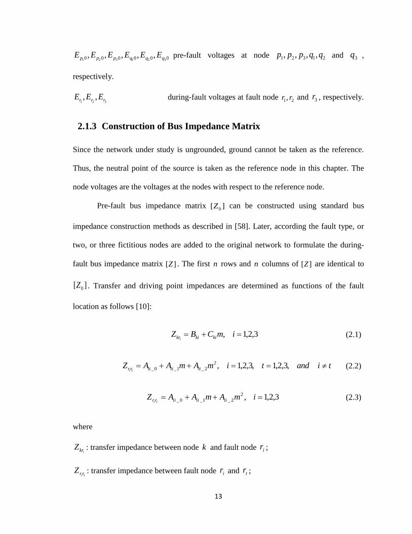
2.1.3 Construction of Bus Impedance Matrix

Since the network under study is ungrounded, ground cannot be taken as the reference.

Thus, the neutral point of the source is taken as the reference node in this chapter. The

node voltages are the voltages at the nodes with respect to the reference node.

Pre-fault bus impedance matrix ][ 0Z can be constructed using standard bus

impedance construction methods as described in [58]. Later, according the fault type, or

two, or three fictitious nodes are added to the original network to formulate the during-

fault bus impedance matrix ][Z . The first n rows and n columns of ][Z are identical to

][ 0Z . Transfer and driving point impedances are determined as functions of the fault

location as follows [10]:

3,2,1, imCBZ kikikri (2.1)

tiandtimAmAAZ itititrr ti ,3,2,1,3,2,1,2

2_1_0_ (2.2)

3,2,1,2

2_1_0_ imAmAAZ iiiiiirr ii (2.3)

where

ikrZ : transfer impedance between node k and fault node ir ;

tirrZ : transfer impedance between fault node ir and tr ;

14

iirrZ : driving point impedance at fault node ir ;

Formulas for 1_0_2_1_0_ ,,,,,, iiiiitititkiki AAAAACB and 2_iiA are shown as follows.

They are constants determined by the network parameters [10].

ikpki ZB (2.4)

)(ii kqkpki ZZC (2.5)

ti ppit ZA 0_ (2.6)

tititi pqqpppitit ZZZzA 21_ (2.7)

itpqqpqqppit zZZZZAtitititi2_ (2.8)

ii ppii ZA 0_ (2.9)

iiii qpppiii ZZzA 221_ (2.10)

iqpqqppii zZZZAiiiiii 22_ (2.11)

Equations (2.1), (2.2) and (2.3) are applicable to one-phase, two-phase and three-

phase line sections.

2.2 Fault Location Methods for Ungrounded Radial

Distribution Systems Using Line to Neutral Voltages and

Line Currents

Figure 2.3 shows a typical ungrounded radial distribution system, which includes one

source, a main feeder, two-phase, three-phase laterals and loads. None of the loads or

sources is connected to the ground. In this section, it is assumed that the neutral point of

15

the source is available, line to neutral voltages and line currents at the substation can be

measured. The neutral point of the source is taken as the reference node here. The

proposed methods aim to pinpoint the fault location occurring on the network [56].

Figure 2.3 A sample ungrounded radial distribution system

Since the original network is ungrounded, the bus impedance matrix of the

network excluding the source impedance is non-existent. Hence, a method is proposed

here to overcome this challenge, presented as below.

Figure 2.4 Modified ungrounded radial system 1

The original ungrounded system is divided into two parts: voltage source with

source impedances and the rest of the network. Figure 2.4 depicts the network without

Rest of

the original

network

addR

addR

addR

ref

ref

ref

add

k

kR

EI 1

1

add

k

kR

EI 2

2

add

k

kR

EI 3

3

1kE

2kE

3kE

1kI

2kI

3kI

1k

2k

3k

Load Load

Load Load

Main feeder

Substation

Source

16

source impedances, where 1k ,

2k and 3k denote substation nodes, 21

, kk EE and 3kE are

during-fault node voltages at substation, and 21

, kk II and 3kI are during-fault line currents

at substation.

Three resistances, symbolized as addR , are added between substation nodes and

the reference node ref , as shown in Figure 2.4. addR can be set to any value; a value of

1-ohm is used in this proposed method.

Then, the bus impedance matrix of the modified system as shown in Figure 2.4

can be obtained by following [58]. Bus impedance matrix of the modified network with

fault nodes being added is then acquired as ][ MZ . Currents flowing into the modified

network can be calculated from the voltages and currents measured at the substation, as

shown in Figure 2.4. Fault location methods are presented as follows.

2.2.1 LL Faults

Consider an LL fault between phase 1 and 2, which could be any two phases out of phase

A, B and C. Name the nodes corresponding to the faulted nodes at substation as 1k and

2k , respectively. Designate ][M as the bus impedance matrix including the fault

resistance of the modified system. ][M can be calculated based on the bus impedance

matrix of modified system without fault resistances ][ MZ [10], [56].

,2

)](:,)(:,)][(:,)(:,[][][

1212211 ___

2121

frrMrrMrrM

T

MMMMM

RZZZ

rZrZrZrZZM

(2.12)

17

where 2211 __ , rrMrrM ZZ and

21_ rrMZ are driving point and transfer impedances of the

modified network, which can be obtained following (2.2) and (2.3). 1f

R is the fault

resistance between fault nodes 1r and

2r . T stands for vector/matrix transpose operator.

The voltage at the substation during the fault can be calculated as

add

k

k

add

k

k

add

k

k

kkkkkk

kkkkkk

kkkkkk

k

k

k

R

EI

R

EI

R

EI

MMM

MMM

MMM

E

E

E

3

3

2

2

1

1

332313

322212

312111

3

2

1

(2.13)

Equation (2.13) can be expanded into three equations, and each equation contains

fault location m and fault resistance1f

R . By rearranging any of the expanded equation,

1fR can be expressed as a function of m . Since

1fR is a real number,

1fR is equal to the

complex conjugate of 1f

R , from which an equation containing only variable m is

obtained. After solving m , and substituting the value of m into the utilized equation, we

can also acquire the value of 1f

R [10].

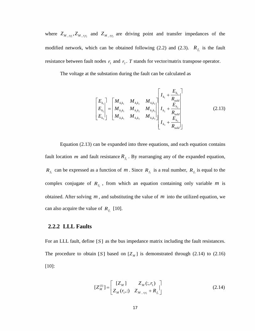
2.2.2 LLL Faults

For an LLL fault, define ][S as the bus impedance matrix including the fault resistances.

The procedure to obtain ][S based on ][ MZ is demonstrated through (2.14) to (2.16)

[10]:

111_1

1)1(

:),(

)(:,][][

frrMM

MM

M RZrZ

rZZZ (2.14)

18

21212211 ___

)1(

2

)1()1(

2

)1(

)1()2(

2

)](:,)(:,)][(:,)(:,[][][

ffrrMrrMrrM

T

NMMNMM

MMRRZZZ

rZrZrZrZZZ

(2.15)

3333

)2(

_

)2(

_

)2(

_

)2(

3

)2()2(

3

)2(

)2(

2

)](:,)(:,)][(:,)(:,[][][

frrMrrMrrM

T

NMMNMM

MRZZZ

rZrZrZrZZS

NNN

(2.16)

where 21

, ff RR and 3f

R are corresponding fault resistances shown in Figure 2.1. Nr is the

node number assigned to the common connection point N of the three fault resistances

under three-phase faults, and 4 nrN .

The voltages at the substation are derived as

add

k

k

add

k

k

add

k

k

kkkkkk

kkkkkk

kkkkkk

k

k

k

R

EI

R

EI

R

EI

SSS

SSS

SSS

E

E

E

3

3

2

2

1

1

332313

322212

312111

3

2

1

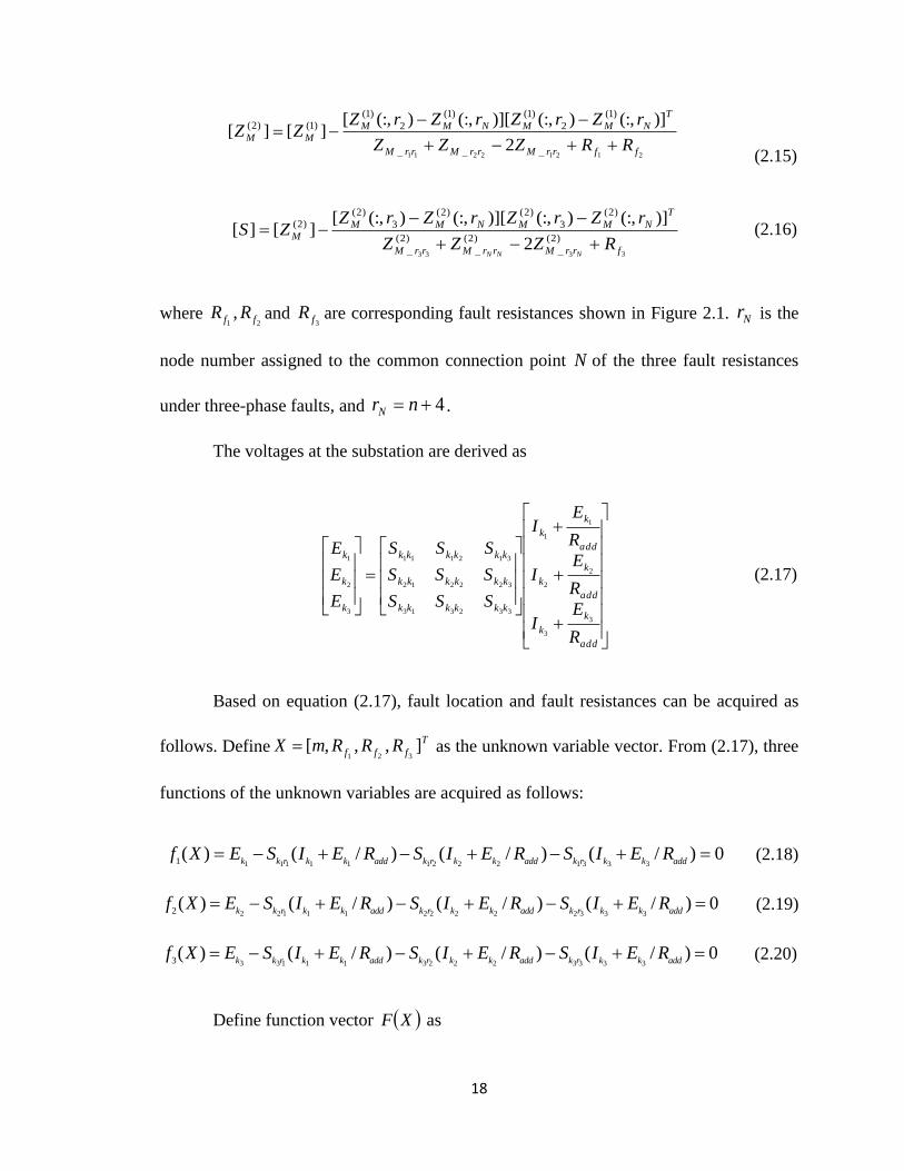
(2.17)

Based on equation (2.17), fault location and fault resistances can be acquired as

follows. DefineT

fff RRRmX ],,,[321

as the unknown variable vector. From (2.17), three

functions of the unknown variables are acquired as follows:

0)/()/()/()(33312221111111

addkkrkaddkkrkaddkkrkk

REISREISREISEXf (2.18)

0)/()/()/()(33322222111222



0)/()/()/()(33332223111333



Define function vector XF as

19

TfimagfrealfimagfrealfimagfrealXF )](),(),(),(),(),([ 332211 (2.21)

where, (.)real and (.)imag represent the real and imaginary part of its argument,

respectively.

Then, the unknown variables can be obtained iteratively through the following

procedure [59]:

X

XFH n

)( (2.22)

)(1

nXFHX (2.23)

nn XXX 1 (2.24)

where

nX is the variable vector for thn iteration;

X is the difference between nX and 1nX ;

H is the Jacobian matrix.

Each element in the Jacobian matrix is calculated from the available node

voltages and line currents at substation, as long with line impedances.

The iterations can be terminated when the biggest element of the unknown

variable update is smaller than the desired tolerance.

20

2.3 Fault Location Methods for Ungrounded Radial

Distribution Systems Using Line to Line Voltages and Line

Currents

This section develops an alternative method for fault location, when line to neutral

voltages is not available, but line to line voltages are available. Methods for both LL and

LLL faults are described.

2.3.1 LL Faults

Figure 2.5 Modified ungrounded radial system 2

To construct the bus impedance matrix, one node at the substation, say node 3k , is

selected as the reference point, as shown in Figure 2.5. Accordingly, phase to phase

voltages can be converted to phase to reference point voltages. The bus impedance matrix

of the original network without source impedances, but with the fictitious fault nodes

added, ][ MZ , can be obtained similarly as in Section 2.2.

Consider an LL fault between phase 1 and 2, which could be any two phases out

of phase A, B and C. Name the nodes corresponding to the faulted nodes at substation 1k

and 2k , respectively. The bus impedance matrix of modified system ][M , including the

fault resistance, can be formulated based on ][ MZ as shown in (2.12).

Rest of

the original

network

1k

2k

3k

1kI

2kI

3kI

1kE

2kE

ref 03kE

21

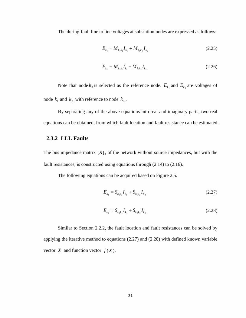
The during-fault line to line voltages at substation nodes are expressed as follows:

2211111 kkkkkkk IMIME (2.25)

2221122 kkkkkkk IMIME (2.26)

Note that node 3k is selected as the reference node. 1kE and

2kE are voltages of

node 1k and 2k with reference to node 3k .

By separating any of the above equations into real and imaginary parts, two real

equations can be obtained, from which fault location and fault resistance can be estimated.

2.3.2 LLL Faults

The bus impedance matrix ][S , of the network without source impedances, but with the

fault resistances, is constructed using equations through (2.14) to (2.16).

The following equations can be acquired based on Figure 2.5.

2211111 kkkkkkk ISISE (2.27)

2221122 kkkkkkk ISISE (2.28)

Similar to Section 2.2.2, the fault location and fault resistances can be solved by

applying the iterative method to equations (2.27) and (2.28) with defined known variable

vector X and function vector )(Xf .

22

2.4 Fault Location Methods for Ungrounded Non-Radial

Distribution Systems Using Line to Neutral Voltages and

Line Currents

Different from ungrounded radial distribution system, ungrounded non-radial distribution

system have an additional source, called remote source, as drawn in Figure 2.6.

Figure 2.6 A sample ungrounded radial distribution system [56]

In the proposed method, it is assumed that the line to neutral voltages and line

currents at the local substation are available. Type I fault location methods proposed in

[10] are applied to ungrounded distribution system in this section. Fault location method

for LL faults will be illustrated here as an example. Detailed approach for LLL faults can

be referred to [10], [56].

2.4.1 LL Faults

Consider an LL fault between phase 1 and 2, which could be phase A and B, or phase B

and C, or phase C and A. Designate the nodes corresponding to the faulted phases at local

substation as 1k and 2k . The voltage change due to the fault at node 1k , or superimposed

voltage at node 1k , is determined by the transfer impedances and fault currents as follows

[10]:

Remote

source

Load Load

Load Load

Main feeder

Local

substation

Local

source

23

221111111 0 frkfrkkkk IZIZEEE (2.29)

Fault currents under LL faults can be obtained by the following form [10], [60]:

1212211

21

21 2

00

frrrrrr

rr

ffRZZZ

EEII

(2.30)

where

1fR fault resistance between node

1r and 2r .

From Figure 2.2, pre-fault voltages at fault node 1r and

2r are determined as

)( 0000 1111 qppr EEmEE (2.31)

)( 0000 2222 qppr EEmEE . (2.32)

Substituting (2.30), (2.31) and (2.32) into (2.29), the following equation is yielded.

])2()2()2[(

])()[(

)]())(1[(

1

1111

21211

2

2_122_222_111_121_221_110_120_220_11

1212

0000

f

kkkk

qqppk

RmAAAmAAAAAA

mCCBB

EEmEEmE

(2.33)

Equation (2.33) is a complex equation, which can be separated into two real

equations. There are two unknowns m and 1f

R . 1f

R is eliminated first and then an

equation involving only m is derived, from which m can be obtained. Then 1f

R can also

be calculated.

24

2.4.2 LLL Faults

DefineT

fff RRRmX ],,,[321

as the unknown variable vector. According to the

method described in [10], three functions of the unknown variable vector can be obtained

as follows:

0)(33122111111 frkfrkfrkk IZIZIZEXf (2.34)

0)(33222211222 frkfrkfrkk IZIZIZEXf (2.35)

.0)(33322311333 frkfrkfrkk IZIZIZEXf (2.36)

By solving equations (2.34), (2.35) and (2.36) using iterative method presented in

Section 2.2.2, fault location and fault resistances can be estimated.

Pre-fault voltage at 121 ,, qpp and 2q can be estimated based on pre-fault node

voltages and currents at the local substation. Approaches calculating node voltages and

branch currents successively from the substation to the end of the feeder are proposed in

[29], [61]. Method presented in [10] is adopted for determining the pre-fault voltage

profiles, shown as follows:

]][[]][[][ 11111 ll IJIJE (2.37)

where

][ 1E pre-fault voltages at local substation;

][ 1I pre-fault currents at local substation;

][ lI pre-fault current injections by the remote source;

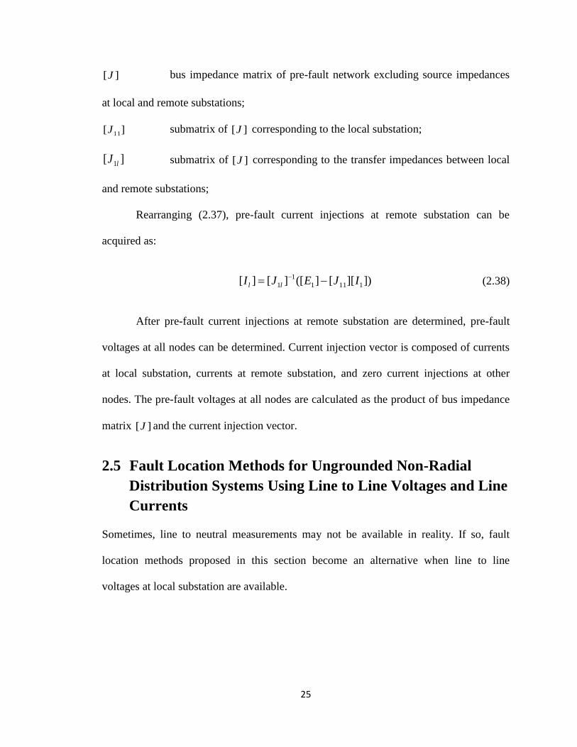
25

][J bus impedance matrix of pre-fault network excluding source impedances

at local and remote substations;

][ 11J submatrix of ][J corresponding to the local substation;

][ 1lJ submatrix of ][J corresponding to the transfer impedances between local

and remote substations;

Rearranging (2.37), pre-fault current injections at remote substation can be

acquired as:

])][[]([][][ 1111

1

1 IJEJI ll (2.38)

After pre-fault current injections at remote substation are determined, pre-fault

voltages at all nodes can be determined. Current injection vector is composed of currents

at local substation, currents at remote substation, and zero current injections at other

nodes. The pre-fault voltages at all nodes are calculated as the product of bus impedance

matrix ][J and the current injection vector.

2.5 Fault Location Methods for Ungrounded Non-Radial

Distribution Systems Using Line to Line Voltages and Line

Currents

Sometimes, line to neutral measurements may not be available in reality. If so, fault

location methods proposed in this section become an alternative when line to line

voltages at local substation are available.

26

2.5.1 LL Faults

Consider an LL fault between phase 1 and 2, which could be any two phases out of phase

A, B and C. Name the nodes corresponding to the faulted nodes at substation 1k and 2k ,

respectively. The voltage change due to the fault from node 1k to node 2k is calculated

as follows [57]:

2222111211212121)()(0 frkrkfrkrkkkkkkk IZZIZZEEE (2.39)

where

21kkE during-fault voltage from node 1k to node 2k ;

021kkE pre-fault voltage from node 1k to node 2k ;

21kkE voltage change from node 1k to node 2k due to the fault.

1212211

2121

21 2

)1( 00

frrrrrr

qqpp

ffRZZZ

mEEmII

(2.40)

where 021ppE is the pre-fault voltage from node 1p to node 2p , 021qqE is the pre-fault

voltage from node 1q to node 2q .

Equation used to estimate the unknown fault location and fault resistance is stated

in (2.41).

])2()2()2[(

])()[(

])1[(

1

22112211

212121

2

2_122_222_111_121_221_110_120_220_11

12121212

00

f

kkkkkkkk

qqppkk

RmAAAmAAAAAA

mCCCCBBBB

mEEmE

(2.41)

27

By separating the above equation into real and imaginary parts, two real equations

can be obtained, and then fault location and fault resistance can be estimated.

2.5.2 LLL Faults

For an LLL fault, the line to line voltage changes due to the fault at substation nodes can

be expressed as

33231222211121121)()()( frkrkfrkrkfrkrkkk IZZIZZIZZE (2.42)

.)()()(33331223211131131 frkrkfrkrkfrkrkkk IZZIZZIZZE (2.43)

Fault currents through fault resistances are given by (2.44) through the matrix

form [10].

0

])1[(

])1[(

111

00

00

1

3131

2121

33133213211131

31322212211121

3

2

1

qqpp

qqpp

frrrrrrrrfrrrr

rrrrfrrrrfrrrr

f

f

f

mEEm

mEEm

RZZZZRZZ

ZZRZZRZZ

I

I

I

(2.44)

By defining the known variable vector X and obtaining function vector )(Xf

based on (2.42) and (2.43), fault location and fault resistances can be obtained following

the similar procedure as stated in Section 2.2.2.

2.6 Evaluation Studies

2.6.1 Fault Location Methods for Ungrounded Radial Distribution

Systems

This section presents evaluation studies to verify the proposed fault location algorithms.

MATLAB package SimPowerSystem is utilized to simulate the studied distribution

28

system [62]. Voltage and current waveforms under different fault types, fault locations

and fault resistances are generated. A 16-bus, 12.47kV, 60Hz ungrounded radial

distribution system, as shown in Figure 2.7, is utilized. Three-phase, two-phase laterals

and loads are involved. A power factor of 0.9 lagging is assumed for all of the loads. Line

length in miles, load ratings in kVA and load phases are labeled. Base values of 12.47kV

and 1MVA are chosen for the per unit system.

Figure 2.7 A sample ungrounded radial power distribution system

Load6

220 kVA

3ø

Load7

120 kVA

2ø (AC)

Load8

200 kVA

2ø (AB)

AB AC

AC BC

BC

Source

15

2.0mi

14

Load5

410 kVA

3ø

Load4

350 kVA

3ø

Load3

100 kVA

2ø (BC)

Load2

160 kVA

2ø (BC)

Load1

320 kVA

3ø

12

1

1.3mi

1.5mi

13

11

10

9 8 7

6 5 4

3

2

2.8mi

1.8mi

1.8mi

1.2mi

1.8mi 2.0mi

1.6mi

2.3mi

3.0mi

1.5mi

1.8mi Load9

100 kVA

2ø (AC)

16 1.7mi

29

Source impedances for each generator in ohms and feeder impedance matrices in

ohms/mile are given as follows, respectively [10], [63].

Source Impedances:

positive-sequence: 0.23 + j2.10

zero-sequence: 0.15 + j1.47

Main feeder impedance matrix:

[0.3465 + j1.0179 0.1560 + j0.5017 0.1580 + j0.4236

0.1560 + j0.5017 0.3375 + j1.0478 0.1535 + j0.3849

0.1580 + j0.4236 0.1535 + j0.3849 0.3414 + j1.0348].

Three-phase lateral feeder impedance matrix:

[0.7526 + j1.1814 0.1580 + j0.4236 0.1560 + j0.5017

0.1580 + j0.4236 0.7475 + j1.1983 0.1535 + j0.3849

0.1560 + j0.5017 0.1535 + j0.3849 0.7436 + j1.2112].

Two-phase lateral feeder impedance matrix:

[1.3294 + j1.3471 0.2066 + j0.4591

0.2066 + j0.4591 1.3238 + j1.3569].

The estimation accuracy of fault location is evaluated by the percentage error

defined in (2.45).

.100%

FeederMaintheofLengthTotal

LocationEstimatedLocationActualError (2.45)

30

where the location of the fault is defined as the distance between the bus with lower index

of the faulty line and the fault point. For example, if the fault occurs on line section

between bus 1 and 2, the fault location is defined as the distance between bus 1 and the

faulted point.

Fault location estimates are acquired by implementing the new algorithms in

MATLAB. For algorithms requiring iterations, initial values of 0.5 per unit for fault

location and 0.005 per unit for fault resistance are adopted. The tolerance of the biggest

element in the unknown variable vector update is set to be 4-101 . In the evaluation

studies, for estimates using iterative approaches, all solutions are acquired within 10

iterations.

Different evaluation studies have been carried out and results are presented in the

rest of this section. The evaluation studies include fault location estimate accuracy

analysis, impacts of load variation on fault location estimates, and sensitivity of fault

location estimates to voltage and current errors.

Typical fault location results for cases with different fault types, fault locations

and fault resistances are presented in Table 2.1 and Table 2.2. Table 2.1 shows fault

location results using line to neutral voltages and line currents at the substation. The first

four columns of Table 2.1 list the actual faulted section, fault type, fault location in per

unit and fault resistance in ohms, respectively. Estimates of fault location errors in

percentage and estimated fault resistances in ohms are listed in the last two columns. In

Table 2.1, the LLL fault on line section 10-12 represents an unbalanced three-phase fault.

Fault resistances [2, 4, 2] indicate that the three interphase fault resistances are 21f

R ,

31

42f

R , and 23f

R , respectively. A fault location error of zero value indicates that

the error is less than 0.0005 in percentage.

Table 2.1 Fault Location Results Using Line to Neutral Voltages and Line Currents

Faulted

section

Fault

type

Fault

location

(per unit)

Fault

resistance

(ohm)

Fault

location

error (%)

Estimated fault

resistance (ohm)

1-2 LL 0.3 5 0 5.002

LLL 0.6 [1,1,1] 0.001 [1.001, 1.001, 1.001]

2-4 LL 0.4 8 0 8.002

LLL 0.7 [10,10,10] 0.001 [10.001,10.001, 10.001]

4-5 LL 0.5 1 0.003 1.001

10-11 LL 0.6 10 0.002 10.002

LLL 0.7 [5,5,5] 0.006 [5.001, 5.001, 5.001]

10-12 LL 0.2 2 0.002 2.003

LLL 0.8 [2,4,2] 0.008 [2.001, 4.001, 2.001]

14-15 LL 0.4 5 0.001 5.002

Fault location results using line to line voltages and line currents at the substation

are displayed in Table 2.2.

It is evinced from Table 2.1 and 2.2 that highly accurate results have been

achieved by the proposed methods. The biggest fault location error occurs when using

line to neutral voltages and line currents at the substation with a LLL fault on line section

10-12. The error is 0.008%, which is still very small.

32

Table 2.2 Fault Location Results Using Line to Line Voltages and Line Currents

Faulted

section

Fault

type

Fault

location

(per unit)

Fault

resistance

(ohm)

Fault

location

error (%)

Estimated fault

resistance (ohm)

1-2 LL 0.4 6 0 6.002

LLL 0.8 [2,2,2] 0.002 [2.001, 2.001, 2.001]

2-3 LL 0.6 3 0 3.002

LLL 0.7 [1,2,1] 0.002 [1.001, 2.001, 1.001]

4-7 LL 0.2 3 0 3.002

LLL 0.3 [3,3,3] 0.004 [3.001, 3.001, 3.001]

7-8 LL 0.7 4 0.002 4.001

10-11

LL 0.7 5 0.003 5.002

LLL 0.6 [2,2,2] 0.006 [2.001, 2.000, 2.001]

14-15 LL 0.8 7 0.001 7.002

Nominal equivalent load impedance is utilized to construct the bus impedance

matrix in methods demonstrated in Sections 2.2 and 2.3. Therefore, actual load variations

in the system may lead to errors in fault location estimation. The impacts of load

variations on fault location estimates have been investigated in the study.

Table 2.3 presents four cases of individual load variations in percentage [10]. In

the first two cases, load levels are decreased and increased by an average of 30%,

respectively. In the last two cases, load levels are decreased and increased by an average

of 20%, respectively.

33

Table 2.3 Individual load variations for ungrounded radial distribution systems

Case

number

Load number

1 2 3 4 5 6 7 8 9

1 -40 -15 -25 -40 -20 -35 -40 -25 -30

2 40 15 25 40 20 35 40 25 30

3 -15 -25 -30 -10 -15 -25 -15 -30 -15

4 15 25 30 10 15 25 15 30 15

In order to mitigate the effects caused by load variations, the following method is

adopted to compensate the load variations. Fault location methods based on line to line

voltages and line currents at the substation are employed here. First, the load level under

the prevailing operating condition is estimated based on the measured pre-fault voltages

and currents at the substation. Then, based on the load level under the nominal condition

and that under the prevailing operating condition, the equivalent load impedances are

scaled as follows [12]:

)()()()( 000000 232131 kkkkkkpwr IEEIEES (2.46)

where pwrS is the complex power injection to the substation preceding the fault and

symbolizes complex conjugate operator. 01kE , 02kE and 03kE are pre-fault voltages at the

substation. 01kI and 02kI are pre-fault line currents flowing out of the substation. Node 3k

is chosen as the reference node here.

Then, the equivalent load impedances are scaled based on the following equation:

34

)(

)( 0

_

pwr

pwr

loadnewloadSreal

SrealZZ (2.47)

where newloadZ _ is the new load impedance, loadZ is the nominal load impedance, and

0pwrS is the power injection to the substation under nominal condition.

The newly obtained load impedances will then be utilized in the construction of

the bus impedance matrix to reflect the load variations. Studies have shown that the load

compensation technique is very effective. As an example, Table 2.4 and Table 2.5 present

fault location errors before and after the mitigation for four cases of load variations given

in Table 2.3. The first three columns of Table 2.4 and Table 2.5 present the actual fault

type, fault location in per unit and fault resistance in ohm, respectively. Estimates of fault

location errors in percentage before and after using mitigation methods are illustrated in

the last four columns. All fault location results in these two tables are based on faults

occurring on line section 10-12, which is a main feeder section.

Table 2.6 and Table 2.7 present fault location errors before and after using the

load compensation method under the same four cases with fault occurring on a lateral

feeder; line section 10-11. Fault location methods based on line to line voltages and line

currents at the substation are also employed here. The first three columns of Table 2.6

and Table 2.7 show the actual fault type, fault location in per unit and fault resistance in

ohm, respectively. Estimates of fault location errors in percentage before and after

employing the mitigation methods are displayed in the last four columns.

35


section 10-12

Fault

type

Fault

location

(per unit)

Fault

resistance

(ohm)

Fault location error (%)

Case 1 Case 2

Before

Mitigation

After

Mitigation

Before

Mitigation

After

Mitigation

LL 0.6 5 0.36 0.06 0.35 0.07

LL 0.3 2 0.24 0.05 0.24 0.06

LLL 0.2 [3,3,3] 0.29 0.08 0.28 0.07

LLL 0.7 [1,1,1] 0.44 0.09 0.41 0.08


section 10-12

Fault

type

Fault

location

(per unit)

Fault

resistance

(ohm)


Case 3 Case 4

Before

Mitigation

After

Mitigation

Before

Mitigation

After

Mitigation

LL 0.6 5 0.21 0.04 0.20 0.04

LL 0.3 2 0.12 0.00 0.12 0.01

LLL 0.2 [3,3,3] 0.15 0.02 0.14 0.01

LLL 0.7 [1,1,1] 0.24 0.03 0.21 0.01

36


section 10-11

Fault

type

Fault

location

(per unit)

Fault

resistance

(ohm)


Case 1 Case 2

Before

Mitigation

After

Mitigation

Before

Mitigation

After

Mitigation

LL 0.7 8 0.20 0.02 0.20 0.01

LL 0.4 2 0.20 0.03 0.19 0.04

LLL 0.3 [2,2,2] 0.25 0.05 0.24 0.05

LLL 0.8 [1,2,1] 0.40 0.05 0.38 0.06


section 10-11

Fault

type

Fault

location

(per unit)

Fault

resistance

(ohm)


Case 3 Case 4

Before

Mitigation

After

Mitigation

Before

Mitigation

After

Mitigation

LL 0.7 8 0.22 0.08 0.21 0.08

LL 0.4 2 0.11 0.01 0.11 0.02

LLL 0.3 [2,2,2] 0.14 0.07 0.13 0.01

LLL 0.8 [1,2,1] 0.24 0.04 0.22 0.03

37

As can be seen from Table 2.4 to 2.7, fault location accuracy has been greatly

improved by utilizing the load compensation approach. Fault location error after

mitigating the impacts of load variation is no larger than 0.09%. Fault location methods

using line to neutral voltages yield very similar results.

The sensitivity of the developed methods to possible voltage and current

measurement errors has also been examined. Scenarios with ± 1% and ± 2% errors

assumed in voltage or current measurements have been studied. Impacts of voltage

measurement errors on fault locations are presented in Table 2.8. Impacts of current

measurement errors on fault locations are shown in Table 2.9. All fault location results in

these two tables are based on faults occurring on line section 2-4.

Table 2.8 Impacts of voltage measurement errors on fault location estimates with fault

occurring on line section 2-4

Fault

type

Fault

location

(per unit)

Fault

resistance

(ohm)


With -1%

voltage

error

With -2%

voltage

error

With 1%

voltage

error

With 2%

voltage

error

LL 0.3 5 0.28 0.56 0.28 0.56

LL 0.6 2 0.34 0.67 0.34 0.67

LLL 0.7 [3,3,3] 0.35 0.70 0.35 0.70

LLL 0.4 [2,1,3] 0.30 0.60 0.30 0.60

38

Table 2.9 Impacts of current measurement errors on fault location estimates with fault

occurring on line section 2-4

Fault

type

Fault

location

(per unit)

Fault

resistance

(ohm)


With -1%

current

error

With -2%

current

error

With 1%

current

error

With 2%

current

error

LL 0.3 5 0.28 0.57 0.28 0.55

LL 0.6 2 0.34 0.68 0.33 0.66

LLL 0.7 [3,3,3] 0.36 0.72 0.34 0.68

LLL 0.4 [2,1,3] 0.30 0.61 0.29 0.58

The first three columns of Table 2.8 and Table 2.9 give the actual fault type, fault

location in per unit and fault resistance in ohm, respectively. Fault location errors in

percentage with ± 1% and ± 2% errors in voltages or currents are presented in the last

four columns. Fault location methods using line to line voltage measurements are utilized

here.

From the above tables, it’s demonstrated that for a ± 2% error in voltage

measurement, fault location errors are within 0.70%, and for a ± 2% error in current

measurement, fault location errors are within 0.72%.

Tables 2.8 to 2.9 have shown that the proposed fault location methods are

insensitive to either voltage or current measurement errors.

39

2.6.2 Fault Location Methods for Ungrounded Non-Radial

Distribution Systems

Figure 2.8 A sample ungrounded power distribution system

This section presents the evaluation studies to verify the proposed fault location

algorithms. MATLAB package named SimPowerSystem is utilized to simulate the

studied distribution system [62]. Voltage and current waveforms under different fault

type, fault location and fault resistance are generated. Voltage and current phasors are

extracted by using Fourier Transform. A 17-bus, 12.47kV, 60Hz ungrounded distribution

Load6

220 kVA

3ø

AC

17

AC BC

BC

Source 2

Source 1

15

2.0mi

1.5mi

14

Load5

410 kVA

3ø

Load4

350 kVA

3ø

Load3

100 kVA

2ø (BC)

Load7

120 kVA

2ø (AC)

Load2

160 kVA

2ø (BC)

Load1

320 kVA

3ø

12

1

1.3mi

1.5mi

13

11

10

9 8 7

6 5 4

3

2

2.8mi

1.8mi

1.8mi

1.2mi

1.8mi 2.0mi

1.6mi

2.3mi

3.0mi

1.5mi

1.8mi Load8

200 kVA

2ø (AB)

AB

Load9

100 kVA

2ø (AC)

16 1.7mi

40

system, as shown in Figure 2.8, is utilized for the evaluation study. Three-phase, two-

phase laterals and loads are involved. A power factor of 0.9 lagging is assumed for all of

the loads. Line length in miles, load ratings in kVA and load phases are clearly labeled.

Both Source 1 and Source 2 are in service. For convenience, base values of 12.47kV and

1MVA are chosen for the per unit system.


MATLAB [62]. The estimation accuracy of fault location is evaluated by the percentage

error defined in (2.45). For algorithms using iterative approaches, initial values of 0.5 per

unit for fault location and 0.005 per unit for fault resistances are adopted. The tolerance

of the biggest element in the unknown variable vector update is set to be 4-101 . In the

studies, for estimates using the iterative methods, all the estimations are obtained within

10 iterations.

Line parameters of the studied 17-bus system are the same as those of the

ungrounded radial distribution system used in Section 2.6.1.Values of source impedances

in ohms are demonstrated as below [10].

Source impedances of source 1:



Source impedances of source 2:



41

The rest of this section presents the fault location results under various studies,

including fault location estimate accuracy analysis, impacts of load variation on fault

location estimates, impacts of voltage and current errors on fault location estimates.

Typical fault location results on different line sections, under different fault types,

fault locations and fault resistances are presented in Table 2.10 and Table 2.11.

Table 2.10 Fault location results using line to neutral voltages at local substation

Faulted

section

Fault

type

Fault

location

(per unit)

Fault

resistance

(ohm)

Fault

location

error (%)

Estimated fault

resistance (ohm)

1-2 LL 0.2 5 0 5.002

LLL 0.5 [2,2,2] 0 [2.001, 2.001, 2.001]

4-7 LL 0.3 10 0.001 10.001

LLL 0.6 [5,5,5] 0 [5.000, 5.001, 5.001]

12-14 LL 0.7 2 0.004 2.001

LLL 0.4 [4,4,4] 0.001 [4.000, 4.001, 4.001]

2-3 LL 0.8 10 0 10.001

LLL 0.3 [2,4,6] 0 [2.001, 4.001, 6.000]

7-9 LL 0.5 1 0 1.002

14-15 LL 0.4 5 0 5.000

Table 2.10 shows the fault location results using line to neutral voltage

measurements at local substation. The first four columns of Table 2.10 list the actual

faulted section, fault type, fault location in per unit and fault resistance in ohms,

42

respectively. Estimates of fault location errors in percentage and estimated fault

resistances in ohms are given in the last two columns. Fault location estimation error

equals 0 indicates the error is less than 0.0005 in percentage.

Fault location results using line to line voltage data at local substation are

displayed in Table 2.11.

Table 2.11 Fault location results using line to line voltages at local substation

Faulted

section

Fault

type

Fault

location

(per unit)

Fault

resistance

(ohm)

Fault

location

error (%)

Estimated fault

resistance (ohm)

2-3 LL 0.1 3 0 3.002

LLL 0.6 [2,3,3] 0 [2.001, 3.001, 3.001]

4-7 LL 0.2 10 0 10.001

LLL 0.4 [1,1,1] 0 [1.001, 1.001, 1.001]

7-9 LL 0.6 4 0.001 4.002

7-10 LL 0.3 8 0.001 8.001

LLL 0.3 [5,5,5] 0 [5.000, 5.001, 5.001]

12-14 LL 0.5 2 0.001 2.001

LLL 0.2 [7,7,7] 0.001 [7.000, 7.001, 7.001]

14-16 LL 0.7 5 0.003 5.002

The biggest fault location estimate error is found when using line to line voltages

at local substation with a LL fault on line section 12-14. The error is 0.004%. It is

43

evinced from Table 2.10 and 2.11 that highly accurate fault location estimates have been

achieved by the proposed methods.

The fault location algorithms proposed in Section 2.4 and 2.5 uses equivalent

impedance of load under nominal condition to build the bus impedance matrix.

Consequently, load variation in the system may results in erroneous fault location. The

influence of load variations on fault location estimates have been investigated in the

study. Table 2.12 presents four cases of individual load variations in percentage [10].

Load levels are decreased by an average of 20% and 30% in the first two cases while load

levels are increased by an average of 20% and 30% in the last two cases.

Table 2.12 Individual load variations for ungrounded distribution systems

Case

number

Load number

1 2 3 4 5 6 7 8 9

1 -15 -25 -30 -10 -15 -25 -15 -30 -15

2 -40 -15 -25 -40 -20 -35 -40 -25 -30

3 15 25 30 10 15 25 15 30 15

4 40 15 25 40 20 35 40 25 30

In order to mitigate the effects caused by load variation, the following method is

adopted to compensate the load variation.

First, the load level under the prevailing operating condition is estimated by using

Equation (2.46). Pre-fault voltage and current measurements at the local substation are

involved. Then, Equation (2.47) is adopted to scale the load impedance based on the load

level under the nominal condition and that under the prevailing operating condition.

44

Table 2.13 and Table 2.14 reveal the effectiveness of the load compensation

technique. Table 2.13 presents fault location estimates before and after the mitigation

process under case 1 and case 2 of load variation. Table 2.14 lists fault location estimates

before and after mitigation process under case 3 and case 4 of load variation. For both

tables, faults occur on line section 7-10. The first three columns of Table 2.13 and Table

2.14 give the actual fault type, fault location in per unit and fault resistance in ohm,

respectively. Estimates of fault location errors in percentage before and after using

mitigation methods are listed in the last four columns. Fault location methods based on

line to line voltages are employed here. Fault location methods using line to neutral

voltages yield similar results.


section 7-10

Fault

type

Fault

location

(per

unit)

Fault

resistance

(ohm)


Case 1 Case 2

Before

Mitigation

After

Mitigation

Before

Mitigation

After

Mitigation

LL 0.7 5 0.36 0.03 0.62 0.04

LL 0.2 2 0.16 0.01 0.28 0.02

LLL 0.3 [3,3,3] 0.39 0.02 0.65 0.03

LLL 0.6 [1,1,1] 0.20 0.02 0.34 0.02

45


section 7-10

Fault

type

Fault

location

(per unit)

Fault

resistance

(ohm)


Case 3 Case 4

Before

Mitigation

After

Mitigation

Before

Mitigation

After

Mitigation

LL 0.7 5 0.36 0.03 0.61 0.05

LL 0.2 2 0.15 0.01 0.27 0.03

LLL 0.3 [3,3,3] 0.38 0.03 0.64 0.05

LLL 0.6 [1,1,1] 0.20 0.02 0.33 0.03

Table 2.15 and Table 2.16 present fault location errors before and after utilizing

the load compensation method under four cases with fault occurring on a three-phase

lateral feeder section; section 12-13. Fault location methods based on line to line voltages

are also employed in this study. The first three columns of Table 2.15 and 2.16 display

the actual fault type, fault location in per unit and fault resistance in ohm, respectively.

Estimates of fault location errors in percentage before and after using mitigation methods

are listed in the last four columns.

46


section 12-13

Fault

type

Fault

location

(per unit)

Fault

resistance

(ohm)


Case 1 Case 2

Before

Mitigation

After

Mitigation

Before

Mitigation

After

Mitigation

LL 0.5 3 0.24 0.02 0.42 0.03

LL 0.8 8 0.45 0.03 0.74 0.03

LLL 0.4 [3,3,5] 0.40 0.01 0.71 0.04

LLL 0.7 [2,2,2] 0.34 0.02 0.58 0.03


section 12-13

Fault

type

Fault

location

(per unit)

Fault

resistance

(ohm)


Case 3 Case 4

Before

Mitigation

After

Mitigation

Before

Mitigation

After

Mitigation

LL 0.5 3 0.24 0.02 0.42 0.05

LL 0.8 8 0.43 0.03 0.73 0.06

LLL 0.4 [3,3,5] 0.40 0.02 0.70 0.06

LLL 0.7 [2,2,2] 0.33 0.02 0.57 0.05

47

As can be seen from these two tables, fault location accuracy has been greatly

improved with the load compensation approach. Fault location error after alleviate the

impacts of load variation is no larger than 0.06%.

The sensitivity of the developed methods to measurement errors has also been

examined. Table 2.17 shows the estimated fault location errors for faults on line section

4-7 with 1% and 2% errors assumed in pre-fault voltage measurements. Impacts of pre-

fault current measurement errors are shown in Table 2.18. The first three columns of

Table 2.17 and Table 2.18 give the actual fault type, fault location in per unit and fault

resistance in ohm, respectively. Fault location errors with ± 1% and ± 2% errors in

voltages or currents are presented in the last four columns.

Table 2.17 Impacts of measurement errors in voltages on fault location estimates with

fault occurring on line section 4-7

Fault

type

Fault

location

(per unit)

Fault

resistance

(ohm)


With -1%

voltage

error

With -2%

voltage

error

With 1%

voltage

error

With 2%

voltage

error

LL 0.2 5 0.04 0.15 0.04 0.18

LL 0.3 2 0.71 1.43 0.72 1.43

LLL 0.3 [1,3,2] 0.48 1.00 0.44 0.85

LLL 0.7 [4,4,4] 0.68 1.15 0.93 2.13

48

Table 2.18 Impacts of measurement errors in currents on fault location estimates with

fault occurring on line section 4-7

Fault

type

Fault

location

(per unit)

Fault

resistance

(ohm)


With -1%

current

error

With -2%

current

error

With 1%

current

error

With 2%

current

error

LL 0.2 5 0.02 0.05 0.02 0.05

LL 0.3 2 0.02 0.04 0.02 0.04

LLL 0.3 [1,3,2] 0.02 0.05 0.02 0.05

LLL 0.7 [4,4,4] 0.03 0.07 0.03 0.07

From the above tables, it’s demonstrated that for a ± 2% error in pre-fault voltage

measurement, fault location errors are within 2.13%, and for a ± 2% error in pre-fault

current measurement, fault location errors are within 0.07%. In fault location methods

proposed in Section 2.4 and 2.5, pre-fault voltages at all nodes are calculated based on the

pre-fault currents at the local and remote substations. Therefore, erroneous pre-fault

currents will lead to incorrect pre-fault voltages at the ends of the faulted line, which

results in incorrect fault location estimates.

Fault location methods using line to line voltage measurements are utilized here.

Fault location methods using line to neutral voltages generate similarly robust results.

49

2.7 Summary

Novel fault location algorithms for both ungrounded radial and non-radial distribution

systems have been presented in this Chapter. Methods using either line to neutral voltages

or line to line voltages are proposed and evaluated for both types of distribution systems.

The proposed fault location methods for radial ungrounded systems utilize only

during-fault voltage and current measurements at the substation. However, pre-fault data

are harnessed to effectively mitigate impacts of load variations. The proposed algorithms

are independent of source impedance, and an approach has been presented for the

construction of bus impedance matrix excluding source impedance.

Fault location methods for non-radial ungrounded distribution systems eliminate

or reduce the need for iterative procedures and yield accurate results.

The network topology change has impacts on fault location accuracy, as on all

existing fault location algorithms. It’s envisioned that the proposed methods can be

implemented as real time online fault location methods. In order to ensure the accuracy of

fault location estimates, network configuration should be updated timely based on

available real time grid monitoring information. An algorithm used for monitoring

network topology changes is referred to [64]. If the network topology changes, the related

information will be transferred to the fault location module for enhanced fault location

accuracy.

Last but not the least, evaluation studies have demonstrated that the proposed

methods produce accurate fault location estimates, and are robust to load variations and

measurement errors.

50

Chapter 3 Distribution System Fault Location Observability

Studies and Optimal Meter Placement

An optimal meter placement scheme for transmission line has been proposed in [48].

Chapter 3 extends the idea to distribution systems. This chapter is organized as follows.

Section 3.1 presents a brief introduction about this section. Section 3.2 describes how to

perform fault location observability analysis. Algorithm of optimal meter placement for

fault location is discussed in Section 3.3. Case studies on a sample power distribution

system are reported in Section 3.4. Conclusions are made in Section 3.5.

3.1 Introduction

Most of the fault location methods developed in the past employ measurements obtained

from a limited number of meters installed in a power system. Optimal meter placement in

power systems is to make the best use of a limited number of meters available to keep the

entire network observable. This section presents fault location observability analysis for

distribution systems, and proposes a novel optimal meter placement algorithm to keep the

system observable in terms of fault location determination. First, the observability of fault

location in power systems is defined. Then analysis of the whole system is performed to

determine the least number of meters needed and the best locations to place those meters

in order to achieve fault location observability. Case studies based on a 16-bus

distribution system have been carried out to illustrate the proposed algorithms.

3.2 Fault Location Observability Analysis

The definition of location observability is illustrated by taking a three-bus sample power

system as an example, as shown in Figure 3.1. In this system, there are three buses and

51

three possible fault locations 21

, FF and3

F . If two different fault locations 1F and

2F

yield the same measurements at a bus, say bus 1, the two fault locations will be

indistinguishable based solely on the measurements at bus 1. In this case, fault locations

1F and 2F are called unobservable. On the contrary, if a unique fault location, say

1F ,

can be deduced based on the measurements at bus 1, and then location 1F is called

observable with the measurements from bus 1. A meter at bus 1 is needed to make

location 1F observable.

Figure 3.1 A sample three-bus power system

In another example, if two possible fault locations 1F and

2F can be derived from

the measurements at bus 1, and two possible fault locations 1F and 3F can be obtained

from the measurements at bus 3. Then the combination of measurements from bus 1 and

bus 3 can lead to the unique fault location 1F . Under this circumstance, fault location

1F

is called observable with the measurements from bus 1 and 3. Meters at bus 1 and 3 are

needed to make location 1F observable.

In order to examine the fault location observability of a network, a fault location

method is needed to estimate the fault location. Any fault location method can be utilized

to perform the fault location observability analysis as long as the type of installed meters

can provide the measurements required for fault location. In this dissertation, a previously

3

1 2 1F

2F

3F

52

proposed fault location method using measurements at a single bus is adopted to perform

the observability analysis [10], which will be reviewed in Section 3.4.

The procedure to determine the observability of a fault location is described as

follows. Suppose that a meter is placed at bus k in the power system. First, suppose that

a specific fault, say an LG fault with a fault resistance of 1 ohm, is posed on a line at

location 1F . Based on the short-circuit analysis, the during-fault measurements at bus k

can be calculated. With the measurements at bus k , the adopted fault location method is

then applied to each line section of the power system, and a set of possible fault locations

on different line sections are obtained, denoted as set kS . If set kS contains only one fault

location, which means fault location 1F can be uniquely determined based on voltage

measurements at bus k , fault location 1F is regarded as observable. If set kS contains

more than one fault location, it indicates that fault location 1F is not observable with the

measurements at bus k .

To make fault location 1F observable, more meters are needed. Now assume that

another meter is placed at another bus, say bus l . Similarly, the voltage measurements at

bus l can be utilized to acquire the corresponding set of possible fault locations lS . The

intersection of kS and lS , denoted as lkS , , gives the most likely fault locations based on

the voltage measurements at bus k and l . If set lkS , contains only one fault location, the

fault point 1F can be uniquely determined based on the voltage measurements at bus k

and l , and fault location 1F is said to become observable. Otherwise, the voltage

measurements at bus k and l are still inadequate to uniquely determine the fault location

1F .

53

Fault location observability can be analyzed similarly for the circumstances where

there are more than two meters installed in a power system.

Generally speaking, if any two different fault locations can be distinguished from

each other by using the available measurements, the system is said to be observable. If

one fault location cannot be distinguished from another fault location with the available

measurements, this fault location is called an unobservable point.

To study the observability of the entire power system, each line of the system is

truncated into short segments of equal length. For instance, if a 2-mile line is truncated

with a resolution of 0.2 mile, 10 segments can be acquired with 11 separate points. By

examining the observability of these 11 points, the observability of this line can be

studied. With the observability of each line in the system being analyzed, the

observability of the entire power system can be determined. If there is any unobservable

point in the system, the system is not observable.

If a meter is available at each bus, then the system will certainly be observable. It

would be desirable to find out the least costly scheme or the minimum number of meters

required keeping the system observable, which is discussed in the following section.

3.3 Optimal Meter Placement Method

To solve the optimal meter placement problem is to find out the optimal locations for

meters to be placed in a system so as to make the entire system observable while the total

cost or the number of meters needed is minimized.

The optimal meter placement problem is formulated as an integer linear

programming problem as follows [48].

54

The optimal meter placement problem can be solved by minimizing the objective

function

n

i

ii McJ1

(3.1)

subject to a set of linear constraints, where ic represents the monitoring cost for a meter

installed at bus i . The value of niMi

,...,1, indicates if a meter is placed at bus i or not.

1iM represents a meter is placed at bus i and 0iM represents no meter is placed at

bus i .

As mentioned in Section 3.2, the fault location observability of the whole power

system is decided by examining the fault location observability of different points in a

distribution system. For each point under certain fault type and fault resistance, a set of

linear constraints can be derived to make this specific fault location observable. To make

the entire power system fully observable, the linear constraints for each fault location

under all fault types and varying fault resistances should be satisfied. Therefore, by

minimizing the value of objective function J subject to all constraints obtained, the

optimal solution can be determined.

The procedure to construct the constraints is illustrated by taking a fault location

1F as an example. First, assume that a fault occurs at location 1F , based on which

measurements at each bus can be obtained through short-circuit analysis. Then, with

measurements at bus nii ,...,1, , a set of possible fault locations, say niSi ,...,1, , can

be acquired by applying the employed fault location method to each line of the power

system. As a result, a total number of n sets can be obtained. Then, the bus

55

number/numbers, whose voltage and current measurements will make 1F observable, are

identified and recorded as follows. First, identify the set with only one element. If set 1i

S

has only one element, it indicates that the measurements at bus 1i can uniquely determine

the fault location1F . The bus number is recorded as }{ 1i . Then, for fault location sets with

two or more elements, obtain the intersection of any two sets, say2i

S and3i

S . If the

intersection 32 ,iiS contains one element, it can be inferred that measurements at bus

2i and

3i are sufficient to uniquely pinpoint the fault location 1F . Record the bus numbers

},{32ii . If the combination of two sets is not enough to uniquely determine fault location

1F , another set can be added to see if the fault location 1F can be uniquely determined.

In this way, all possible sets of meters to make 1F observable can be identified.

Based on all the obtained sets with recorded bus number/numbers, the constraints

of the optimization problem are then constructed. An example is provided here to explain

the procedure. Suppose that there is a four-bus power system, with buses numbered 1, 2,

3 and 4. For a studied fault location, by applying the above method to the system, three

sets of buses are yielded: {1, 2}, {1, 3}, {4}. It indicates that if there are meters at buses 1

and 2, or at buses 1 and 3, or solely at bus 4, the studied fault location can be uniquely

determined. Based on the definition of )...,，1( niMi

, the above statement can be

represented by the following constraint:

1)()(43121 MMANDMMANDM (3.2)

where AND represents the logical AND operator.

Equation (3.2) can be transformed to linear constraints as shown in [48].

56

To make a power system fully observable, one should first derive the constraints

corresponding to a certain fault location under a specified type of fault and fault

resistance. Then constraints for all the other fault locations and resistances under the

same fault type can be acquired similarly. In the end, one can derive the constraints for all

fault locations under all types of faults and fault resistances. By minimizing the objective

function subject to all of the constraints, the optimal meter placement problem can be

solved.

3.4 Fault Location Methods

In this section, a previously proposed fault location method using measurements at a

single bus is reviewed, and utilized to perform the observability analysis.

The proposed fault location methods for LG, LL, LLG, LLL and LLLG faults

have been derived respectively, as can be referred to [10]. Fault location approaches for

LG will be illustrated here as an example. Methods for other types of faults can be found

in [10]. The same notations used in Section 2.1.2 are utilized here for consistency.

However, it should be noted that in this chapter, 21,kk and 3k represents nodes

corresponding to the faulted phases at the bus with a meter. They no longer present the

nodes corresponding to the faulted phases at the substation. Figure 3.2 depicts the

diagram of LG, LLG and LLLG faults, where fictitious nodes representing the fault

points on the faulty line are named ,, 21 rr and 3r , respectively. Figure 2.2 demonstrate a

fault occurring on a three-phase line section with fictitious nodes drawn on each phase.

The construction of bus impedance matrix can be referred to descriptions in Section 2.1.3.

57

In this study, an LLL or an LLLG fault can either be a balanced fault or an unbalanced

fault.

Figure 3.2 Diagrams of LG, LLG and LLLG faults

3.4.1 LG Faults

For an LG fault with the faulted phase being phase A, B, or C, designate the node

corresponding to the faulted phase at the bus with a meter as 1k . The voltage change due

to the fault at node 1k , or superimposed voltage at node 1k , is calculated as [10]:

111111 0 frkkkk IZEEE (3.3)

where

ikE during-fault voltage at node ik ;

0ikE pre-fault voltage at node ik ;

ikE voltage change at node ik due to the fault;

1r

1fR

2fR

3fR

2r

1r

2r

3r

1fR

1r

1fR

2fR

LG faults

LLG faults

gRgR

LLLG faults

58

ifI fault current flowing through the fault resistance out of the fault node ir .

It’s negative of current injection.

Fault current can be obtained by the following form [58], [60]:

111

1

1

0

frr

r

fRZ

EI

(3.4)

where

1fR fault resistance between node

1r and the ground.

From Figure 2.2, pre-fault voltage at fault node 1r can be acquired as shown in

(2.31). 01pE and 01qE can be determined after pre-fault voltage profile is obtained

following the procedure described in Section 2.4.2.

Substituting (2.31) and (3.4) into (3.3), the following equation is yielded for

estimating the unknown fault location.

)()(

112

2_111_110_11

000

1

111 mCBRmAmAA

EEmEE

iii kk

f

qpp

k

(3.5)

where )3,2,1(,,,,,,,2_1_0_2_1_0_11

iAAAAAACBiiiiiiitititikik are constants given in Section 2.1.2,

which are determined by the network parameters.

By separating (3.5) into real and imaginary parts, two real equations can be

obtained, from which the fault location m can be estimated.

For LLG, LLL and LLLG faults, one should choose suitable unknown variable

vector X and construct related function vector )(XF . Then, fault location can be

estimated using the iterative method discussed in Section 2.2.2.

59

By applying the above fault location method to each line section of the system, a

list of likely fault location estimates may be generated, comprising the true estimate and

the fake estimates. Depending on available measurements, some of the fake estimates

may be eliminated as illustrated in Section 3.5.1, while other fake estimates may be

indistinguishable from the true fault location.

3.5 Evaluations studies

Figure 3.3 A sample power distribution system

C

15

AB

Load6

200 kVA

3ø

A B

BC

Source

2.0mi

14

Load5

400 kVA

3ø

Load4

350 kVA

3ø

Load3

100 kVA

1ø (B)

Load7

150 kVA

1ø (A)

Load2

160 kVA

2ø (BC)

Load1

300 kVA

3ø

12

1

1.3mi

1.5mi

13

11

10

9 8 7

6 5 4

3 2

2.8mi

1.8mi

1.8mi

1.2mi

1.8mi 2.0mi

1.6mi

2.3mi

1.9mi

1.5mi

1.8mi

Load8

150 kVA

2ø (AB)

Load9

110 kVA

1ø (C)

16 1.7mi

60

This section presents the case studies and results of the proposed methods for performing

fault location observability analysis and optimal meter placement. A 16-bus, 12.47kV,

60Hz distribution system, as shown in Figure 3.3, is utilized for the study, with detailed

system parameters referred to [63]. The system is a typical distribution system including

unbalanced lateral feeders and loads of single-phase, two-phase or three-phase. A lagging

power factor of 0.9 is assumed for all the loads. Line length in miles, load ratings in kVA

and load phases are labelled. A resolution of 0.2 mile is used for studying fault location

observability. Base values of 12.47kV and 1MVA are selected for the per unit system.

Studies for faults with different types including LG, LL, LLG, LLL, LLLG faults

have been carried out. For ground faults, fault resistances of 1, 50, 100 ohms are used.

For other fault types, fault resistances of 1 and 5 ohms are employed.

In the following sections, a method to reduce or eliminate multiple possible fault

location estimates to reach a unique estimate is first discussed in Section 3.5.1. Then,

Section 3.5.2 presents the fault location observability analysis results. The optimal meter

placement results are reported in Section 3.5.3.

3.5.1 Method to Trim Multiple Fault Location Estimates

As mentioned in Section 3.2, for a specific fault, with voltage measurements available at

one given bus, several possible fault locations on different lines may be acquired. Except

the actual fault location, other fault locations are called fake fault locations. The

following example illustrates why fake fault locations exist. Suppose that an AG fault

with a 1 ohm fault resistance is posed at 1.2 miles away from bus 7 on line section 7-8 in

the system. Voltages at bus 7 are considered as known measurements. By using the

measurements, four fault location estimates are obtained as presented in Table 3.1.

61

Table 3.1 Fake fault location analysis results under an AG fault with a 1-ohm fault

resistance on line section 7-8

Fault

location

Number

Estimated

fault location

(mile)

Voltage difference between

measured and calculated

voltage at bus 7 (per unit)

1 [2, 3, 0.67] {0, 0.1055, 0.0938}

2 [4, 6, 1.07] {0, 0.0232, 0.0207}

3 [7, 8, 1.20] {0, 0, 0}

4 [7, 10, 1.49] {0, 0.0037, 0.0037}

The significance of Table 3.1 is explained below.

In order to closely examine these four fault locations, the following procedure is

performed to analyze each fault location estimate.

1. Assume a fault does occur at the estimated fault location.

2. Perform short-circuit analysis to calculate the during-fault voltages at the

bus providing measured voltages, which is bus 7 in this case. The voltages calculated in

this step are designated as calculated voltages, which are used to be compared with the

measured voltages employed to calculate the fault location estimate.

3. Compare the measured and calculated voltages at the bus with the

measured voltages, i.e., bus 7.

62

Table 3.1 shows the results of above analysis on the four estimated fault locations.

The first, second and third columns list the fault location number, estimated fault location

in miles, and per unit voltage differences between the measured and calculated during-

fault voltages in three phases. Fault location 1 - [2, 3, 0.67] represents a fault at 0.67

miles away from bus 2 on line section 2-3. {0, 0.1055, 0.0938} denotes the differences

between the measured and calculated voltages in per unit at bus 7 for phase A, B and C,

respectively. Other fault location estimates in Table 3.1 can be interpreted similarly. The

third fault location estimate is the true value and the other three locations are fake

estimates.

Table 3.1 manifests that all the four fault location estimates have the same

calculated phase A voltage at bus 7, which is expected. This is because the fault location

method utilized only during-fault phase A voltage for an AG fault, and phase B and C

voltages are not used. Thus, comparison of the measured voltages with the calculated

ones may help identify certain fake fault locations as follows.

For a fault location estimate, if the calculated voltages are different from the

measured voltages, this fault location is considered as a fake one. In this chapter, a

tolerance of 0.01 per unit is adopted to judge whether two values are different or not, with

consideration of potential measurement errors. According to this criterion, in Table 3.1,

fault locations 1 and 2 are identified as fake locations. Fault location 4 is

indistinguishable from the true fault location using only the voltage measurements. So,

not all fake fault locations can be identified.

When available, measured line currents will be adopted to further reduce the

number of fake fault locations. For a fault location estimate 1F with measurements

63

available from bus k , if the calculated voltages and currents at bus k are different from

measured voltages and currents at bus k , this fault location is a fake one. To simplify the

procedure, the problem of comparing a branch current is transformed into comparing the

voltages at both ends of the branch. A tolerance of 0.01 per unit is used.

Another example is provided below to further elucidate that utilizing both

voltages and currents will help eliminate fake estimates. Table 3.2 gives fault location

estimates with measurements available at bus 10. A BG fault with a fault resistance of 50

ohms occurs at 0.7 miles away from bus 7 on line section 7-10. In Table 3.2, the first

column lists the case number, and the second column displays the estimated fault

locations. Case 1 represents the circumstances where only voltage measurements are

utilized to calculate the fault location and no fake fault locations are eliminated. In case 2,

fake fault locations are removed by comparing calculated voltages based on estimated

fault location with measured voltages at bus 10. In case 3, fake fault locations are

eliminated by comparing calculated measurements, including both voltages and currents,

with measured measurements at bus 10. Since a meter is installed at bus 10, current

flowing from bus 10 to 7, 10 to 11 and 10 to 12 are assumed to be known. All these three

branch currents are used to determine the fake fault locations in case 3.

It can be seen from Table 3.2, that five possible fault locations are acquired in

case 1 with measurements at bus 10. In case 2, by comparing the calculated and measured

voltages at bus 10, fault location [2, 3, 1.24] has been detected as a fake fault location,

and removed from fault location list. In case 3, three more fault locations are removed

when compared to case 2. Only the actual fault location is left. It’s evinced that some

64

fake fault locations can be eliminated by taking advantage of both voltages and currents

at the bus with measurements.

Table 3.2 Fault location results under three different cases under a BG fault with a 50-

ohm fault resistance on line section 7-10

Case Number Estimated fault location (mile)

1

[2, 3, 1.24]

[4, 5, 0.42]

[4, 6, 0.49]

[7, 9, 0.24]

[7, 10, 0.70]

2

[4, 5, 0.42]

[4, 6, 0.49]

[7, 9, 0.24]

[7, 10, 0.70]

3 [7, 10, 0.70]

In the following sections, both voltage and current measurements are utilized to

eliminate fake fault locations. It will be shown that to eliminate all the fake fault location

estimates, it may be necessary to install more meters in the system.

3.5.2 Fault Location Observability Analysis Results

In the study, if the difference between two calculated possible fault locations is less than

0.01 mile, the two fault locations will be considered to be the same estimate. This

criterion helps to determine whether a fault location exists in the intersection of two fault

65

location sets discussed in Section 3.2. Representative observability study results are

shown as follows.

Figure 3.4 Unobservable segments under AG faults with a 50-ohm fault resistance with a

meter placed at bus 1

Suppose that only one meter is placed at bus 1 and voltages and currents at bus 1

are measured. The fault location observability analysis has been performed. Figure 3.4

depicts the analysis results for AG faults with a fault resistance of 50 ohms. The

unobservable segments of the studied system are marked with black rectangles, with the

length of each unobservable segment being labelled. Remaining segments are observable.

Please notice AG fault is not applicable to line 4-5, 7-9, or 14-16, since these lines do not

15 14

12

1

13

11 10

9 8 7

6 5 4

3 2

16

1.3mi

1.5mi

1.8mi

1.5mi

1.2mi

1.8mi

2.1mi

1.8mi

1.6mi

1.8mi

Unobservable segment

66

have phase A. From Figure 3.4, it is shown that many of the lines are unobservable if

there is only one meter placed at bus 1.

Figure 3.5 Unobservable segments under AG faults with a 50-ohm fault resistance with

meters placed at buses 1 and 3

Figure 3.5 shows unobservable segments under AG faults with a 50-ohm fault

resistance after another meter is placed at bus 3. It demonstrates that the unobservable

segments have been significantly reduced after adding a meter to the system.

To further explicate the impact of the number of measurements on fault location

observability, Table 3.3 presents estimated fault locations under BG faults with a 1-ohm

fault resistance under different meter placements. The first column gives the actual fault

15 14

12

1

13

11 10

9 8

7

6 5 4

3 2

16

0.3mi

1.5mi

0.3mi

0.3mi

0.5mi

1.8mi

0.5mi

0.1mi

Unobservable segment

67

location. The second and third columns list the estimated fault locations using

measurements at buses 5 and 6, respectively. The last column presents the estimated fault

locations with meters placed at both buses 5 and 6. For fault location [2, 3, 0.30], a meter

at bus 5 or bus 6 alone is enough to make this fault location observable. For the fault

location of 0.2 miles from bus 4 to 7, employing measurements at bus 5, two possible

fault locations can be calculated: one being 0.25 miles from bus 4 to 6, and the other

being 0.20 miles from bus 4 to 7. Utilizing measurements at bus 6 alone also yields two

estimates. The combination of measurements at buses 5 and 6 leads to a unique fault

location, which is 0.20 miles from bus 4 to 7. So, meters at both buses 5 and 6 are needed

to make this fault location observable. For the third fault location, meters at buses 5 and 6

are insufficient to make the fault location observable.

Table 3.3 Fault location set under BG faults with a 1-ohm fault resistance

Actual

Fault location

(mile)

Estimated fault

location (mile)

/Bus 5

Estimated fault

location (mile)

/ Bus 6

Estimated fault

location (mile)

/ Bus 5 and 6

[2, 3, 0.3] [2, 3, 0.30] [2, 3, 0.30] [2, 3, 0.30]

[4, 7, 0.2] [4, 6, 0.25]

[4, 7, 0.20]

[4, 5, 0.20]

[4, 7, 0.20]

[4, 7, 0.20]

[12, 14, 0.3] [12, 13, 0.23]

[12, 14, 0.30]

[12, 13, 0.23]

[12, 14, 0.30]

[12, 13, 0.23]

[12, 14, 0.30]

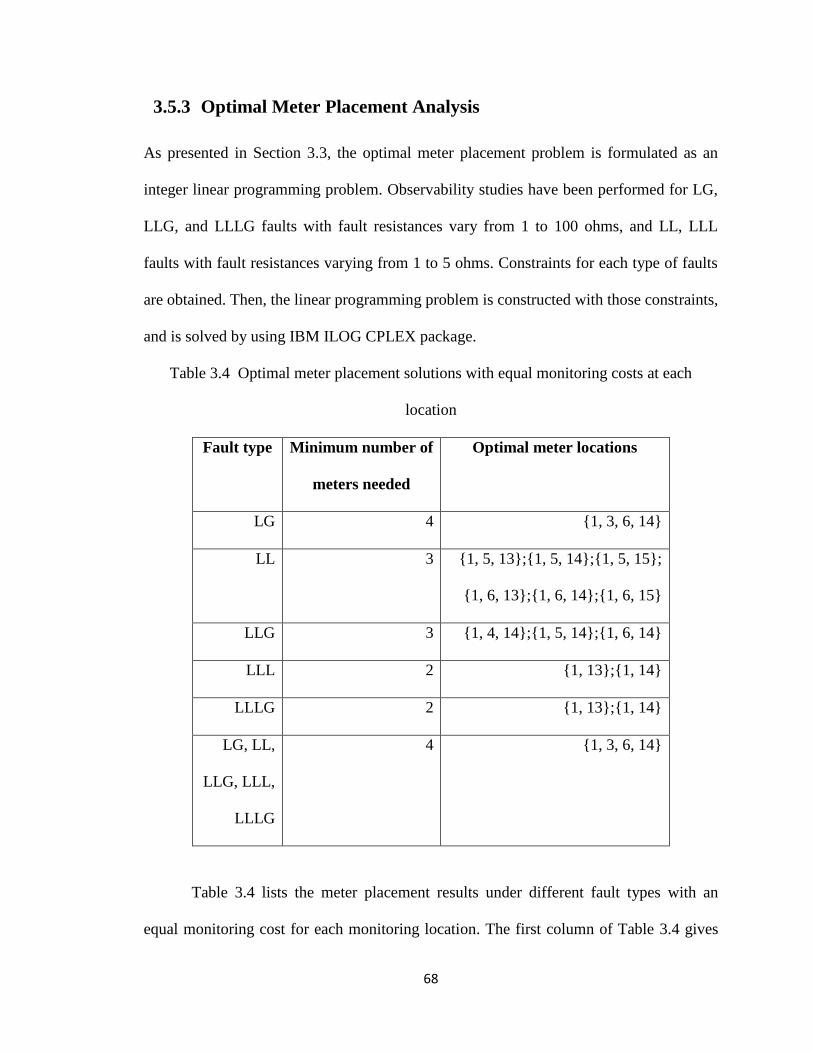
68

3.5.3 Optimal Meter Placement Analysis

As presented in Section 3.3, the optimal meter placement problem is formulated as an

integer linear programming problem. Observability studies have been performed for LG,

LLG, and LLLG faults with fault resistances vary from 1 to 100 ohms, and LL, LLL

faults with fault resistances varying from 1 to 5 ohms. Constraints for each type of faults

are obtained. Then, the linear programming problem is constructed with those constraints,

and is solved by using IBM ILOG CPLEX package.

Table 3.4 Optimal meter placement solutions with equal monitoring costs at each

location

Fault type Minimum number of

meters needed

Optimal meter locations

LG 4 {1, 3, 6, 14}

LL 3 {1, 5, 13};{1, 5, 14};{1, 5, 15};

{1, 6, 13};{1, 6, 14};{1, 6, 15}

LLG 3 {1, 4, 14};{1, 5, 14};{1, 6, 14}

LLL 2 {1, 13};{1, 14}

LLLG 2 {1, 13};{1, 14}

LG, LL,

LLG, LLL,

LLLG

4 {1, 3, 6, 14}

Table 3.4 lists the meter placement results under different fault types with an

equal monitoring cost for each monitoring location. The first column of Table 3.4 gives

69

the fault type. The second column lists the minimum number of meters that are needed.

Optimal meter locations are presented in the last column.

In this study, it is assumed that a meter is always placed at substation (bus 1),

which is usually the case in practice. As a result, meter placement results for each fault

type have a “1” in meter location set. It’s demonstrated that four meters are needed to

make the system observable for LG faults, three meters are required for LL and LLG

fault, and only two meters are enough to uniquely locate any LLL or LLLG faults. The

last row indicates that, to make the system observable under all types of fault, at least

four meters are needed to be deployed at bus 1, 3, 6, and 14, respectively.

It should be noticed that the optimal meter placement yields the least number of

meters and the locations to place the meters so as to make the system observable.

Therefore, any meter placement set that contains the optimal meter set also has the ability

to make the system observable. For example, a set of meters at bus {1, 5, 13} can

uniquely determine any LL fault, then a set of meters at bus {1, 5, 13, k }

)13,5,116,...,1( kandk can definitely pinpoint any LL fault uniquely. Besides,

multiple optimal meter placements may exist for some fault types. For instance,

according to Table 3.4, there are six optimal solutions for LL faults.

Sometimes, the monitoring expenses at different locations may not be the same. It

may be easier to install a meter at a certain location, and therefore the monitoring cost

will be lower at this location. Or, if a meter is needed at a location for multiple purposes

such as fault location and power quality monitoring, the monitoring cost for this location

will be lower to represent a higher need. Different monitoring costs will impact the

optimal meter placement solution as shown below.

70

Table 3.5 shows the optimal meter placement results for LL faults under different

monitoring cost distributions. The first column indicates the case number. The second

column presents the monitoring costs at each location. The third and fourth columns list

the minimum number of meters needed and their locations.

Table 3.5 Optimal meter placement solutions for LL faults with varying monitoring

coasts at each location

Case

number

Monitoring

costs

Minimum

number of

meters needed

Optimal meter locations

1 ic is equal for

16,...,1i

3 {1, 5, 13};{1, 5, 14};{1, 5, 15}

{1, 6, 13};{1, 6, 14};{1, 6, 15}

2 26 c , 1ic for

others

3 {1, 5, 13};{1, 5, 14};{1, 5, 15}

3 26 c , 5.114 c ,

1ic for others

3 {1, 5, 13};{1, 5, 15}

4 21 c , 1ic for

others

3 {1, 5, 13};{1, 5, 14};{1, 5, 15}

{1, 6, 13};{1, 6, 14};{1, 6, 15}

Based on the results, it is demonstrated that the optimal meter placement solutions

may differ if the monitoring cost for each location varies. By comparing case 2 with case

1, it is noticed that the meter placement solutions with bus 6 are no longer optimal

solutions since the monitoring cost at bus 6 is higher than that at other locations. In the

71

third case, the monitoring cost at bus 14 is increased, and as a result, the optimal meter

placement solutions containing bus 14 are removed when compared to the solutions of

the second case. In case 4, although the monitoring cost at bus 1 is higher than others, the

optimal meter placement solutions still contain bus 1. The reason for this is that a meter

at bus 1 is mandatory, and 11 M . So no matter how high the monitoring cost is, bus 1 is

always included in the optimal solutions.

3.6 Summary

This chapter presents fault location observability analysis for distribution systems. Case

studies indicate that when limited measurements are available, multiple fault location

estimates may exist, which may be impossible to distinguish from the true fault location.

Potential techniques by using captured voltage and current measurements are described to

trim multiple fault location estimates. To achieve fault location observability of the entire

system, sufficient meters are needed to be placed at different locations. An optimal meter

placement scheme is proposed to make the distribution system observable while

minimizing the total cost or the number of needed meters. The obtained results may

provide guidance on installing meters for fault location purposes.

72

Chapter 4 Optimal Fault Location Estimation in Distribution

Systems with DG

A method to optimally estimate fault location on transmission lines is proposed in [59].

This chapter investigates optimal fault location estimation method for distribution

systems with DG. In this study, an optimal fault location estimator is presented. It is

assumed that measurements at location/locations with power generation are available.

This location can either be the substation or location with DG. Approach to detect and

identify bad measurement is presented for enhanced accuracy of fault location estimation.

4.1 Fault Location Method

In order to construct the optimal fault location estimator, a fault location method is

needed. A previously proposed fault location method described in [10] is employed here

for the optimal fault location estimator. The fault location algorithm for LG fault is

demonstrated here as an instance. Procedure to find out fault location for other types of

fault can be referred to [10]. In this section, it is assumed that measurements at a location

with power generation are available. Three nodes at this location are denoted as 21,kk and

3k ,respectively.

Based on Figure 2.2, 1r is added to the faulted phase as the fault node under an

LG fault. The voltage change due to the fault at node 3,2,1, iki , or superimposed

voltage at node ik , is given as follows [10]:

)()(

112

2_111_110_11

000

1

111 mCBRmAmAA

EEmEE

iii kk

f

qpp

k

(4.1)

73

For the superimposed voltages and currents due to fault at a location with power

generation, the following relationship holds [10].

][][][ IZE s (4.2)

where

][ E the three-phase voltage changes due to fault at the location with power

generation;

][ I the three-phase current changes due to fault at the same location;

][ sZ the source impedance matrix of the source at the same location.

4.2 Optimal Fault Location Estimation

As we know, measurements obtained by recording devices may have errors. Inaccurate

measurement data will lead to inaccurate fault location estimates. In order to eliminate

the impacts of measurement errors on fault location estimates, an optimal estimator for

fault location is proposed in this section. The proposed optimal fault location estimator is

capable of detecting and identifying bad measurements.

Optimal fault location estimator for LG faults with available measurements is

illustrated here as an example. Optimal fault location estimators for other types of faults

can be derived similarly, are not presented here. The study of testing the effectiveness of

the optimal fault location estimator is presented in Section 4.4.

Suppose the following vector S is formulated based on the available

superimposed voltage and current data caused by the fault:

T

kkkk NNIIEES ],...,,,...,[

3131 (4.3)

where

74

N total number of buses with voltage and current

measurements available;

NiEEEiii kkk ,...,2,1,,,

31323

superimposed voltages at bus i , with nodes

iii kkk 31323 ,, , caused by the fault;

NiIIIiii kkk ,...,2,1,,,

31323

superimposed currents at bus i , with nodes

iii kkk 31323 ,, , caused by the fault.

Define the unknown variable vector X as

],,...,[ 212112122,1 NNN xxxxxX (4.4)

where

Nix i 6,...,0,12 magnitude of iS ; iS is the thi element of S ;

Nix i 6,...,0,2 angle of iS ;

112 Nx fault location variable;

212 Nx fault resistance variable.

For an LG fault with voltage and current measurements at bus i , Ni ,...,0 , three

variable functions (4.5), (4.6), (4.7) can be acquired based on (4.1) and three variable

functions (4.8), (4.9), (4.10) can be acquired based on (4.2).

0))](([

)()(

11000

2

2_111_110_1123

2323111

123

mCBEEmE

RmAmAAEXf

ii

i

kkqpp

fki (4.5)

0))](([

)()(

11000

2

2_111_110_1113

1313111

1

mCBEEmE

RmAmAAEXf

ii

i

kkqpp

fki (4.6)

75

0))](([

)()(

11000

2

2_111_110_113

33111

1

mCBEEmE

RmAmAAEXf

ii

i

kkqpp

fki (4.7)

0)3,1()2,1()1,1()(3132323 ___233

iiii kiskiskiskiN IZIZIZEXf (4.8)

0)3,2()2,2()1,2()(3132313 ___133


0)3,3()2,3()1,3()(313233 ___33


where isZ _ is the source impedance matrix of the source at bus i . ),(_

baZis represents

the element in the th

a row and th

b column of isZ _ .

From the above derivation, it’s known that with measured data at one bus, six

variable functions can be formulated. Therefore, a total number of N6 variable functions

can be constructed based on measurement at N buses.

Define measurement vector Y as

NiYi 12,...,1,0 (4.11)

NiSY iiN 6,...,1,1212 (4.12)

NiSY iiN 6,...,1212 (4.13)

where . and . represent the magnitude and angle in radiance of the input argument,

respectively.

Construct function vector )(XF as

76

T

NNN xxxffffffXF ],...,,),Im(),Re(),...,Im(),Re(),Im(),[Re()( 1221662211

(4.14)

where Re(.) and Im(.) represent the real and imaginary part of the input argument,

respectively. Both Y and )(XF have a size of 1 by N24 .

The vector of measurement errors is defined as the difference between

measurement vector and function vector as given in (4.15).

)(XFY (4.15)

The optimal estimate of X can be achieved with minimized cost function J ,

which is the determined by the weighting matrix W and measurement errors.

)]([)]([ XFYWXFYJ T (4.16)

where the weighing matrix W is the inverse of the covariance matrix R , defined as

],...,,[][ 2

4

2

2

2

1 N

T diagER (4.17)

In the above equation, ].[E gives the expected value of the input argument.

(.)diag is a diagonal matrix with the values in the square brackets. 2

i indicates the error

variance of measurement i . The meter with smaller error variance is more accurate.

First, reasonable values for each variable are assigned to X as the initial variable

vector0X . Then, (4.15) is solved iteratively with X being updated by the following

procedure [68].

77

kXXX

XFH

)( (4.18)

)]}([{)( 111

k

TT

k XFYRHHRHX (4.19)

kkk XXX 1 (4.20)

where

k iteration number starting from 1;

kX variable vector at thk iteration;

kX variable update during the thk iteration.

Finally, the optimal solution of X is obtained when the biggest element in the

variable update is smaller than the desired tolerance.

4.3 Bad Data Detection

In this dissertation, the Chi-square test is used to determine whether or not bad data exist

in the measurement set. The expected value of the cost function is equal to the degrees of

freedom K .

)()( HrowHcolK (4.21)

where (.)col and (.)row signify the number of columns and rows of the input argument,

respectively.

The estimated cost function

J can be calculated by the following expression:

78

N

i i

iJ1

2

2

(4.22)

where

i

estimated measurement error in measurement i ;

2

i variance of the error in measurement i ;

N total number of measurements.

The Chi-square test, demonstrated in [68], is adopted to determine the presence of

a bad data. The Chi-square value with specified probability P of confidence and degrees

of freedom K can be found according to the Chi-square distribution table. If 2

,PKJ

,

then bad data will be suspected with probability P . For example, if 2

%95,KJ

, it means

in 95% of the cases, a bad data exist in the measurements. Then, the measurement with

the largest standardized error is identified as the bad data. Otherwise, for cases where

2

,PKJ

, the measurement sets are assumed to be free of bad data.

In our study, 0.99 is chosen for P to construct a 99% confidence interval.

4.4 Evaluation Studies

This section presents the evaluation studies on the proposed fault location algorithms. A

18-bus, 12.47kV, 60Hz distribution system, as shown in Figure 4.1, is utilized for the

evaluation study. Besides the source at substation, distributed generation are placed at bus

11 and 18, respectively. Single-phase, two-phase, and three-phase laterals and loads are

involved. A power factor of 0.9 lagging is assumed for all of the loads. Line length in

miles, load ratings in kVA and load phases are clearly labeled. For convenience, base

79

values of 12.47kV and 1MVA are chosen for the per unit system. In the study, initial

values for variable vector are chosen as: 1.0 p.u. for measurement magnitude, 0 radians

for measurement angle, 0.5 p.u. for fault location and 0.005 p.u. for fault resistances.

Figure 4.1 A sample power distribution system with DG

DG2

DG1

C

17

A B

BC

Substation

source

15

2.0mi

1.5mi

14

Load5

400 kVA

3ø

Load4

350 kVA

3ø

Load3

100 kVA

1ø (B)

Load2

160 kVA

2ø (BC)

Load1

300 kVA

3ø

12

1

1.3mi

1.5mi

13

11

10

9 8 7

6 5

4

3

2

2.8mi

1.8mi

1.8mi

1.2mi

1.8mi 2.0mi

1.6mi

2.3mi

3.0mi

1.5mi

1.8mi Load8

150 kVA

2ø (AB)

AB

Load9

110 kVA

1ø (C)

16 1.7mi

Load10

370 kVA

3ø

18 1.5mi

Load7

150 kVA

1ø (A)

Load6

200 kVA

3ø

80


MATLAB [62]. MATLAB tool package SimPowerSystems is utilized to model the

studied 18-bus system and generates voltage and current measurements at the substation

and locations with DG [62]. Due to different meter accuracies, 610 and 410 are chosen

as the variance for the first N12 measurements and last N12 measurements of Y ,

respectively. In the studies, all the solutions are reached within 10 iterations.

Source impedances for each generator are given as follows. Impedance matrices

of main feeders and later feeders in ohms/mile are listed in [63].

Source impedances of substation source:

positive-sequence: 0.23 + j2.10 ohm

zero-sequence: 0.15 + j1.47 ohm

Source impedances of DG1:



Source impedances of DG2:



The estimation accuracy is evaluated by the percentage error is given in (2.45).

The rest of this section presents the fault location results under various studies.

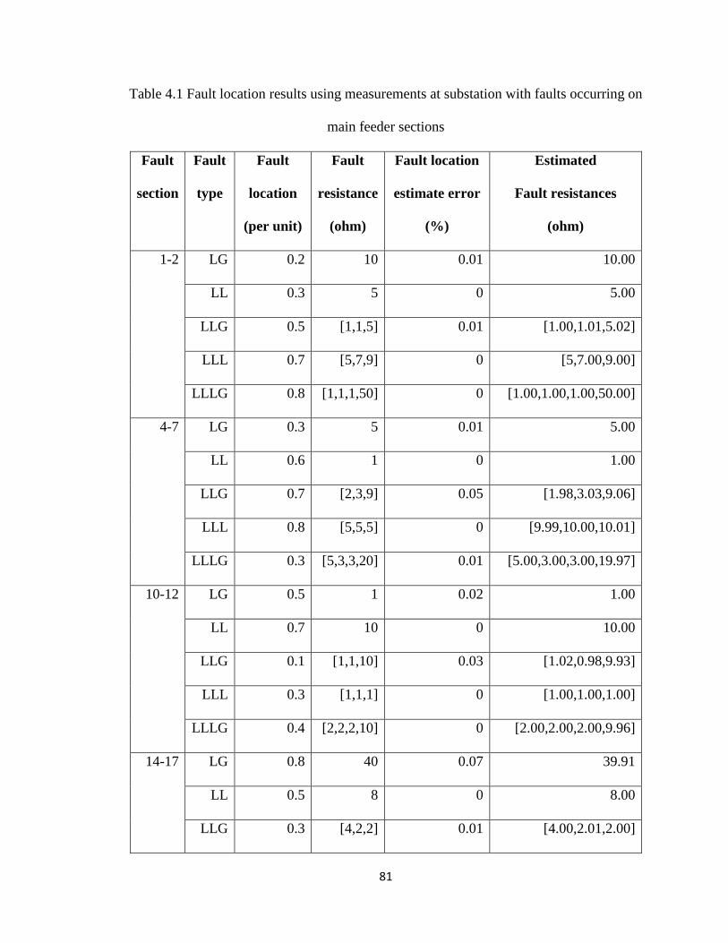
81


main feeder sections

Fault

section

Fault

type

Fault

location

(per unit)

Fault

resistance

(ohm)

Fault location

estimate error

(%)

Estimated

Fault resistances

(ohm)

1-2 LG 0.2 10 0.01 10.00

LL 0.3 5 0 5.00

LLG 0.5 [1,1,5] 0.01 [1.00,1.01,5.02]

LLL 0.7 [5,7,9] 0 [5,7.00,9.00]

LLLG 0.8 [1,1,1,50] 0 [1.00,1.00,1.00,50.00]

4-7 LG 0.3 5 0.01 5.00

LL 0.6 1 0 1.00

LLG 0.7 [2,3,9] 0.05 [1.98,3.03,9.06]

LLL 0.8 [5,5,5] 0 [9.99,10.00,10.01]

LLLG 0.3 [5,3,3,20] 0.01 [5.00,3.00,3.00,19.97]

10-12 LG 0.5 1 0.02 1.00

LL 0.7 10 0 10.00

LLG 0.1 [1,1,10] 0.03 [1.02,0.98,9.93]

LLL 0.3 [1,1,1] 0 [1.00,1.00,1.00]

LLLG 0.4 [2,2,2,10] 0 [2.00,2.00,2.00,9.96]

14-17 LG 0.8 40 0.07 39.91

LL 0.5 8 0 8.00

LLG 0.3 [4,2,2] 0.01 [4.00,2.01,2.00]

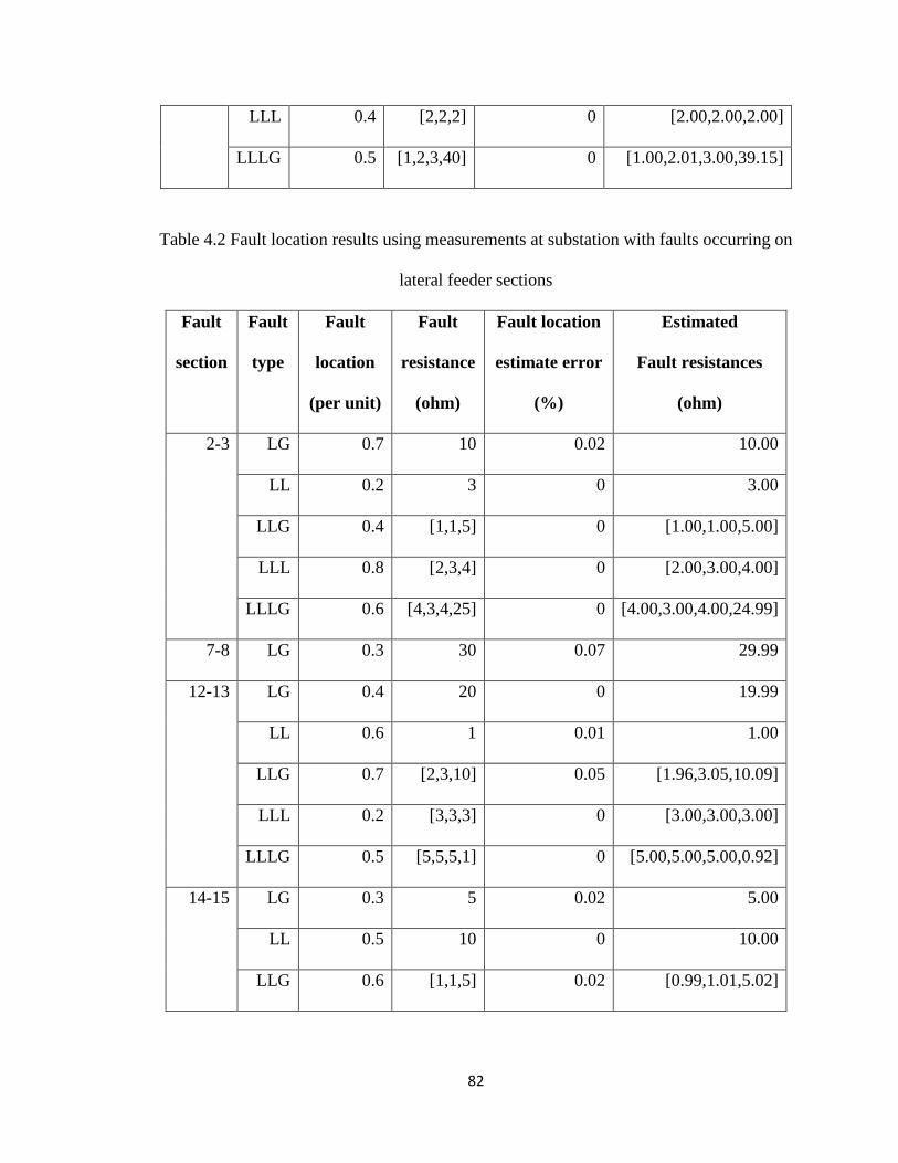
82

LLL 0.4 [2,2,2] 0 [2.00,2.00,2.00]

LLLG 0.5 [1,2,3,40] 0 [1.00,2.01,3.00,39.15]


lateral feeder sections

Fault

section

Fault

type

Fault

location

(per unit)

Fault

resistance

(ohm)

Fault location

estimate error

(%)

Estimated

Fault resistances

(ohm)

2-3 LG 0.7 10 0.02 10.00

LL 0.2 3 0 3.00

LLG 0.4 [1,1,5] 0 [1.00,1.00,5.00]

LLL 0.8 [2,3,4] 0 [2.00,3.00,4.00]

LLLG 0.6 [4,3,4,25] 0 [4.00,3.00,4.00,24.99]

7-8 LG 0.3 30 0.07 29.99

12-13 LG 0.4 20 0 19.99

LL 0.6 1 0.01 1.00

LLG 0.7 [2,3,10] 0.05 [1.96,3.05,10.09]

LLL 0.2 [3,3,3] 0 [3.00,3.00,3.00]

LLLG 0.5 [5,5,5,1] 0 [5.00,5.00,5.00,0.92]

14-15 LG 0.3 5 0.02 5.00

LL 0.5 10 0 10.00

LLG 0.6 [1,1,5] 0.02 [0.99,1.01,5.02]

83

Fault location results on different line sections, under different fault types, fault

locations and fault resistances are presented in Table 4.1 and Table 4.2. Table 4.1 shows

the fault location results using measurements at substation with faults on main feeders.

Table 4.2 shows the fault location results using measurements at substation with faults on

lateral feeders. The first four columns of Table 4.1 give the actual faulted section, fault

type, fault location in per unit and fault resistance in ohms, respectively. Estimates of

fault location errors and estimated fault resistances are given in the last two columns.

Both balanced and unbalanced LLL and LLLG faults are considered in the study. In this

section, fault location estimation error equals 0 indicates the error is less than 0.005 in

percentage.

From the above tables, it is evinced that accurate results have been achieved by

the proposed optimal fault location estimator. Biggest fault location error is 0.07%.

Fault location results using voltage and current data at substation and locations

with DG are displayed in Table 4.3 and 4.4. Fault location estimation under the same

faults as those shown in Table 4.1 and 4.2 are displayed in Table 4.3 and 4.4, respectively.

From Table 4.3 and 4.4 it is learned that, accuracy of fault location estimates can be

enhanced if more measurements are available. All fault location errors are within 0.07%.

84


with faults occurring on main feeder sections

Fault

section

Fault

type

Fault

location

(per unit)

Fault

resistance

(ohm)

Fault location

estimate error

(%)

Estimated

Fault resistances

(ohm)

1-2 LG 0.2 10 0.01 10.00

LL 0.3 5 0 5.00

LLG 0.5 [1,1,5] 0 [1.00,1.01,5.02]

LLL 0.7 [5,7,9] 0 [5.00,7.00,9.00]

LLLG 0.8 [1,1,1,50] 0 [1.00,1.00,1.00,50.00]

4-7 LG 0.3 5 0.01 5.00

LL 0.6 1 0 1.00

LLG 0.7 [2,3,9] 0 [1.99,3.01,8.98]

LLL 0.8 [5,5,5] 0 [10.00,10.00,10.00]

LLLG 0.3 [5,3,3,20] 0 [5.00,3.00,3.00,19.99]

10-12 LG 0.5 1 0 1.00

LL 0.7 10 0 10.00

LLG 0.1 [1,1,10] 0.02 [1.00,1.00,10.00]

LLL 0.3 [1,1,1] 0 [1.00,1.00,1.00]

LLLG 0.4 [2,2,2,10] 0 [2.00,2.00,2.00,10.00]

14-17 LG 0.8 40 0.05 40.01

LL 0.5 8 0 8.00

LLG 0.3 [4,2,2] 0.01 [4.00,2.00,2.00]

85

LLL 0.4 [2,2,2] 0 [2.00,2.00,2.00]

LLLG 0.5 [1,2,3,40] 0 [1.00,2.00,3.00,40.22]


with faults occurring on lateral feeder sections

Fault

section

Fault

type

Fault

location

(per unit)

Fault

resistance

(ohm)

Fault location

estimate error

(%)

Estimated

Fault resistances

(ohm)

2-3 LG 0.7 10 0.01 10.00

LL 0.2 3 0 3.00

LLG 0.4 [1,1,5] 0 [1.00,1.00,5.00]

LLL 0.8 [2,3,4] 0 [2.00,3.00,4.00]

LLLG 0.6 [4,3,4,25] 0 [4.00,3.00,4.00,25.00]

7-8 LG 0.3 30 0.07 30.01

12-13 LG 0.4 20 0 20.00

LL 0.6 1 0 1.00

LLG 0.7 [2,3,10] 0.02 [1.99,3.01,9.99]

LLL 0.2 [3,3,3] 0 [3.00,3.00,3.00]

LLLG 0.5 [5,5,5,1] 0 [5.00,5.00,5.00,0.988]

14-15 LG 0.3 5 0 5.00

LL 0.5 10 0 10.00

LLG 0.6 [1,1,5] 0 [1.00,1.00,5.00]

86

The effectiveness of the proposed optimal estimator in detecting and identifying

existing bad measurement has been studied and results are demonstrated as follows.

Suppose that an AG fault with 0.3 p.u. fault location and 5 Ohm fault resistance takes

place on line section 4-7 of the simulated power system. Measurements at the local

substation are employed for the optimal fault location estimator.

After voltage and current measurements are extracted from MATLAB model, the

voltage magnitude of phase A at substation is deliberately multiplied by 1.5 to generate a

bad measurement. Optimal estimations of all variables in the variable vector with bad

measurement are presented in Table 4.5. Optimal estimations of variables after the bad

data is removed are displayed in Table 4.6. The first three columns of Table 4.5 and 4.6

list the available measurements, measurement units, measured values, respectively.

Optimal estimates of all variables are given in the last column.

According to (2.45), fault location error is obtained as 14.47%, which is

considerably large. After calculating the cost function and looking up in the table for Chi-

square distribution, it can be acquired that 1007.9491

J and 23.2093 2

99.0,10 . Since

2

, pkJ

, a bad measurement is detected. Searching for the measurement with the biggest

standard error, bad measurement is identified as the measured voltage magnitude of

phase A at the local substation. After eliminating the bad data, and use the rest data to

perform optimal estimation again, the results in Table 4.6 are obtained. “N/A” indicates

the corresponding value is not available.

87


measurement at 1E

Quantity Unit Measured

values

Optimal

estimates

1E per unit 0.2157 0.2925

1E radians -2.3658 -2.3659

2E per unit 0.0373 0.0399

2E radians 0.7856 0.7855

3E per unit 0.0330 0.0370

3E radians 0.7433 0.7435

1I per unit 0.1741 0.2113

1I radians -0.6876 -0.6876

2I per unit 0.0122 0.0129

2I radians 2.5047 2.5047

3I per unit 0.0089 0.0103

3I radians 2.4009 2.4009

m per unit 0.3000 -1.4359

fR per unit 3.2154 2.7166

88


measurement removed


values

Optimal

estimates

1E per unit N/A 0.2157

1E radians -2.3658 -2.3659

2E per unit 0.0373 0.0374

2E radians 0.7856 0.7857

3E per unit 0.0330 0.0330

3E radians 0.7433 0.7433

1I per unit 0.1741 0.1741

1I radians -0.6876 -0.6876

2I per unit 0.0122 0.0122

2I radians 2.5047 2.5047

3I per unit 0.0089 0.0090

3I radians 2.4009 2.4009

m per unit 0.3000 0.3023

fR per unit 3.2154 3.2142

89

After removing the bad data, the newly calculated cost function 0.0193

J and

20.0902 2

99.0,8 . Fault location error after bad data being removed is 0.02%. As a

result, the new measurement sets are considered free of bad data, and the fault location

estimate is shown to be very accurate. Optimal estimates of variables based on

measurements at substation and locations with DG are also very accurate.

Optimal estimates with error in current measurements have also been tested.

Suppose the same fault, AG fault with 0.3 p.u. fault location and 5 Ohm fault resistance,

occurs in the system. Bad measurement is generated by multiplying the current

magnitude of phase A by 1.5. All other measurements are accurate. Optimal estimations

of all variables in the variable vector with bad measurement are presented in Table 4.7.

By comparing the values of estimated cost function and Chi-square value,

measured current magnitude of phase A at the local substation is detected with

measurement error. Optimal estimation results after removing the bad data are listed in

Table 4.8.

90


measurement at 1I


values

Optimal

estimates

1E per unit 0.2157 0.2457

1E radians -2.3658 -2.3659

2E per unit 0.0373 0.0380

2E radians 0.7856 0.7856

3E per unit 0.0330 0.0343

3E radians 0.7433 0.7434

1I per unit 0.1741 0.2243

1I radians -0.6876 -0.6876

2I per unit 0.0122 0.0072

2I radians 2.5047 2.5047

3I per unit 0.0089 0.0043

3I radians 2.4009 2.4009

m per unit 0.3000 -0.5305

fR per unit 3.2154 3.0142

91


measurement removed


values

Optimal

estimates

1E per unit 0.2157 0.2157

1E radians -2.3658 -2.3658

2E per unit 0.0373 0.0374

2E radians 0.7856 0.7857

3E per unit 0.0330 0.0330

3E radians 0.7433 0.7433

1I per unit N/A 0.1741

1I radians -0.6876 -0.6877

2I per unit 0.0122 0.0122

2I radians 2.5047 2.5047

3I per unit 0.0089 0.0089

3I radians 2.4009 2.4009

m per unit 0.3000 0.3008

fR per unit 3.2154 3.2146

92

After current magnitude of phase A being eliminated from the measurement pool,

no other bad data are found based on the newly calculated cost function and Chi-square

value. As can be seen from Table 4.8, fault location estimate is very accurate.

Optimal fault location estimation based on measurements at substation and

locations with DG yield similar accurate results.

4.5 Summary

This chapter describes a novel optimal fault location estimator for distribution systems

with DG. Voltage and current measurements at substation with/without measurements at

locations with DG are utilized to give the best estimation of all available measurements

along with fault location and fault resistances. Functions of superimposed measurements,

fault location and fault resistance are obtained based on the characteristics of the system.

Then, estimation of all variables is evaluated iteratively. Simulation studies have

demonstrated that highly accurate estimates are obtained. If a bad measurement exists in

the measured data, the proposed method is able to detect and identify this bad

measurement successfully. Fault location estimates after removing the bad data from the

data pool are very accurate.

93

Chapter 5 Conclusions

Faults on power systems may result in discontinue of electricity, which will do harm to

schools, hospitals, and public safety entities including, police stations, fire department,

law enforcement agencies, etc. Failure of power also brings the country financial losses.

Impedance based fault location methods for radial and non-radial ungrounded

distribution systems are proposed in Chapter 2. Fault location methods using line to

neutral voltages at substation are presented first. When line to line to neutral voltages are

not available due to physical connection inside the sources, fault location approaches

using line to line voltages at substation are utilized as an alternative. Voltages at

substation nodes are formulated as the functions of bus impedance matrix and current at

the substation. Bus impedance matrix contains the fault location to be determined. By

solving the constructed function with measured voltages at the substation, fault location

can be estimated. For both radial and non-radial ungrounded distribution systems, fault

location methods for LL and LLL faults are designed, where the former ones do not have

to be solved iteratively. In fault location methods for non-radial ungrounded distribution

systems, pre-fault node voltages and source impedance is not required. Evaluations

studies on 12.47 kV 16-bus radial system and 17-bus non-radial system are carried out.

Accurate fault location estimates are obtained by both methods. The proposed fault

location methods are very robust to load variation and measurement data with errors.

Due to presence of multi-laterals in distribution systems, and limited monitoring

devices, it may be inherently impossible to uniquely determine some fault locations. In

other words, there may be multiple fault location estimates if only a limited

measurements are available, and all such estimates satisfy the given network conditions

94

and measurements. Optimal meter placement method to minimize the number of meters

needed while make every fault location uniquely determinable by available measurement.

In this dissertation, an optimal meter deployment problem is converted into an integer

linear programming, as shown in Chapter 3. At first, the constraints corresponding to a

certain fault location under a specified type of fault and fault resistance is formulated.

Then, the constraints for all the other fault locations and resistances under the same fault

type can be acquired similarly. In the end, the constraints for all fault locations under all

types of faults and fault resistances are obtained. By minimizing the objective function

subject to all of the constraints, the optimal meter placement problem can be solved. All

constrains are formulated based on the results of fault location observability analysis. An

existing fault location algorithm is adopted for fault location observability study, and

measurements at only one bus are required to find the fault location. Fault location

methods for LG, LL, LLG, LLL and LLLG are presented. Evaluation studies are

performed on a 12.47kV 16-bus distribution system. For a fault location in the system,

measured voltages at one bus may results in two or more possible fault locations. In this

case, more meters are needed to make the actual fault location observable. Evaluation

studies demonstrate that the length and number of unobservable segments in the system

can be largely reduced by installing more meters in the system. To make the entire

studied distribution system observable, four meters are needed at specific locations. In

other words, four meters at specified locations are enough to locate any fault in the

system.

A method to optimally estimate the unknown fault location in distribution systems

is described in Chapter 4. The proposed methods employ voltage and current

95

measurements at substation with/without locations with DG to determine the best

estimation of measurements, fault location and fault resistances. Optimal estimation of all

variables, including fault location, fault resistances and measurements, are acquired by

iteratively solve the functions obtained based on the characteristic of the system. Very

accurate fault location estimates are obtained according to the evaluation studies. This

dissertation also provides a method to detect and identify bad measurement if there is any

in the measured data. Evaluation study indicates that bad measurement can be detected

by comparing the value of cost function with the Chi-square value. Then, bad date is

identified as the one with largest standardized error. After removing the bad

measurement from the measurement poor, and use the rest of the measurements to

estimate fault location again, very accurate fault location estimates are obtained.

96

References

[1] D. Jalali and N. Moslemi, “Fault location for radial distribution system using fault

generated high-frequency transients and wavelet analysis,” 18th International

Conference and Exhibition on Electricity Distribution, Turin, Italy, June 6-9, 2005.

[2] J. Sadeh, E. Bakhshizadeh, and R. Kazemzadeh, “New fault location algorithm for

radial distribution systems using modal analysis,” International Journal of Electrical

Power and Energy Systems, vol. 45, pp. 271-278, February 2013.

[3] A. M. El-Zonkoly, “Fault diagnosis in distribution networks with distributed

generation,” Electric Power Systems Research, vol. 81, no. 7, pp. 1482-1490, July

2011.

[4] L. Zewen, H. Huanhuan and D. Feng, “Power grid fault traveling wave network

location method,” 2013 IEEE Industry Applications Society Annual Meeting, Lake

Buena Vista, FL, October 06-11, 2013.

[5] H. Nouri, C. Wang, and T. Davies, “An accurate fault location technique for

distribution lines with tapped loads using wavelet transform,” IEEE Porto Power

Tech Conference, Porto, Portugal, September 10-13, 2001.

[6] H. Li, A. S. Mokhar, and N. Jenkins, “Automatic fault location on distribution

network using voltage sags measurements,” 18th International Conference and

Exhibition on Electricity Distribution, Turin, Italy, June 6-9, 2005.

[7] R. A. F. Pereira, L. G. W. Silva, M. Kezunovic, and J. R. S. Mantovani, “Improved

fault location on distribution feeders on matching during-fault voltage sags,” IEEE

Transactions on Power Delivery, vol. 24, no. 2, pp. 852-862, April 2009.

97

[8] S. Lotfifard, M. Kezunovic, and M.J. Mousavi, “Voltage sag data utilization for

distribution fault location,” IEEE Transactions on Power Delivery, vol. 26, no. 2, pp

1239-1246, April 2011.

[9] N. Kang; Y. Liao, “Fault location estimation for transmission lines using voltage sag

data,” 2010 IEEE Power and Energy Society General Meeting, Minneapolis, MN,

July 25-29, 2010.

[10] Y. Liao, “Generalized fault-location methods for overhead electric distribution

systems,” IEEE Transactions on Power Delivery, vol. 26, no. 1, pp. 53-64, January

2011.

[11] R. Das, M. S. Sachdev, and T. S. Sidhu, “A fault locator for radial sub-

transmission and distribution lines,” 2000 IEEE Power Engineering Society Summer

Meeting, Seattle, Washington, July 16-20, 2000.

[12] R. K. Aggarwal, Y. Aslan, and A. T. Johns, “New concept in fault location for

overhead distribution systems using superimposed components,” IEE Proceedings on

Generation, Transmission and Distribution, vol. 144, no. 3, pp. 309-316, May 1997.

[13] R. K. Aggarwal, Y. Aslan, and A. T. Johns, “An interactive approach to fault

location on overhead distribution lines with load taps,” 6th

International Conference

on Developments in Power System Protection, pp. 184-187, Nottingham , March 25-

27, 1997.

[14] A. L. Dalcastagne, S. N. Filho, H. H. Zurn, and R. Seara, “An iterative two-

terminal fault-location method based on unsynchronized phasors,” IEEE Transaction

on Power Delivery, vol. 23, no. 4, pp. 2318–2329, October 2008.

98

[15] J. Kim, M. Baran, and G. Lampley, “Estimation of fault location on distribution

feeders using PQ monitoring data,” IEEE Power Engineering Society General

Meeting, Tampa, FL, June 24-28, 2007.

[16] J. Teng, W. Huang and S. Luan, “Automatic and fast faulted line-section location

method for distribution systems based on fault indicators,” IEEE Transactions on

Power Systems, vol. 29, no. 4, pp. 1653-1662, July 2014.

[17] S. Lotfifard, M. Kezunovic, and M. J. Mousavi, “A systematic approach for

ranking distribution systems fault location algorithms and eliminating false

estimates,” IEEE Transactions on Power Delivery, vol. 28, no. 1, pp. 285-293,

January 2013.

[18] J. Zhu, D. L. Lubkeman, and A. A. Girgis, “Automated fault location and

diagnosis on electric power distribution feeders,” IEEE Transactions on Power

Delivery, vol. 2, no. 2, pp. 801-809, April 1997.

[19] R. Krishnathevar and E. E. Ngu, “Generalized impedance-based fault location for

distribution systems,” IEEE Transactions on Power Delivery, vol. 27, no. 1, pp. 449-

451 January 2012.

[20] G. Morales-España, J. Mora-Flórez, and H. Vargas-Torres, “Elimination of

multiple estimation for fault location in radial power systems by using fundamental

single-end measurements,” IEEE Transactions on Power Delivery, vol. 24, no. 3, pp.

1382-1389, July 2009.

[21] F. Yan, W. Liu, and L. Tian, “Fault location for 10kV distribution line based on

traveling wave-ANN theory,” 2011 IEEE Power Engineering and Automation

Conference, vol. 2, pp. 437-440, September 8-9, 2011.

99

[22] L. S. Martins, J. F. Martins, C. M. Alegria, and V. Femilo Pires, “A network

distribution power system fault location based on neural eigenvalue algorithm,” 2003

IEEE Bologna Power Tech Conference, Bologna, Italy, June 23–26, 2003.

[23] F. Dehghani and H. Nezami, “A new fault location technique on radial

distribution systems using artificial neural network,” 22nd International Conference

and Exhibition on Electricity Distribution, pp. 1-4, Stockholm, June 10-13, 2013.

[24] J. J. Mora, G. Carrillo, and L. Perez, “Fault location in power distribution systems

using ANFIS nets and current patterns,” 2006 IEEE/PES Transmission and

Distribution Conference and Exposition: Latin America, pp. 1–6, Caracas, August 15-

18, 2006.

[25] X. Zhu, X. Lu, D. Liu, and B. Zhang, “An improved fault locating system of

distribution network based on fuzzy identification,” 2010 China International

Conference on Electricity Distribution, pp. 1-6, Nanjing, China, September 13-16,

2010.

[26] J. Mora-Florez, V. Barrera-Nuez, and G. Carrillo-Caicedo, “Fault location in

power distribution systems using a learning algorithm for multivariable data

analysis,” IEEE Transactions on Power Delivery, vol. 22, no. 3, pp.1715-1721, July,

2007.

[27] M. M. Hosseini, M. T. Hagh, and S. Asgarifar, “A novel fault location algorithm

for double fed distribution networks,” IEEE Power Engineering and Automation

Conference (PEAM), 2011.

100

[28] M. S. Choi, S. J. Lee, D. S. Lee, and B. G. Jin, “A new fault location algorithm

using direct circuit analysis for distribution systems,” IEEE Transactions on Power

Delivery, vol. 19, no. 1, pp. 35-41, January 2004.

[29] M. S. Choi, S. J. Lee, S. I. Lim, D. S. Lee, and X. Yang, “A direct three-phase

circuit analysis-based fault location for line-to-line fault,” IEEE Transactions on

Power Delivery, vol. 22, no. 4, pp. 2541-547, October 2007.

[30] A. A. Girgis, C. M. Fallon, and D. L. Lubkeman, “A fault location technique for

rural distribution feeders,” IEEE Transactions on Industry Applications, vol. 29, no.

6, pp. 1170-1175, November/December 1993.

[31] G. D. Ferreira, D. S. Gazzana, A. S. Bretas, and A. S. Netto, “A unified

impedance-based fault location method for generalized distribution systems,” Power

and Energy Society General Meeting, San Diego, CA, July 2012.

[32] D. Novosel, D. Hart, and J. Myllymaki, “System for locating faults and estimating

fault resistance in distribution networks with tapped loads,” U.S. Patent 5839093,

1998.

[33] T. A. Kawady, A.-M. I. Taalab and M. El-Sad, “An accurate fault locator for

underground distribution networks using modified apparent-impedance calculation,”

10th IET International Conference on Developments in Power System Protection, pp.

1-5, Manchester, March 29-April 1, 2010.

[34] S. Kulkarni, S. Santoso, and, T. A. Short, “Incipient Fault Location Algorithm for

Underground Cables,” IEEE Transactions on Smart Grid, vol. 5, no. 3, pp. 1165-

1174, May 2014.

101

[35] T. S. Sidhu; Z. Xu, “Detection of Incipient Faults in Distribution Underground

Cables,” IEEE Transactions on Power Delivery, vol. 25, no. 3, pp. 1363-1371, July

2010.

[36] Z. Xu, “Fault location and incipient fault detection in distribution cables,” Ph.D.

dissertation, Electrical and Computer Engineering, University of Western Ontario,

London, Ontario, 2011.

[37] J. Moshtagh and R.K. Aggarwal, “A new approach to ungrounded fault location

in a three-phase underground distribution system using combined neural networks

and wavelet analysis,” 2006 Canadian Conference on Electrical and Computer

Engineering, pp. 376-381, Ottawa, ON, Canada, May 2006.

[38] S. Nam, S. Kang, J. Sohn, and J. Park, “Ground-fault location algorithm for

ungrounded radial distribution systems”, Electrical Engineering, vol. 89, no. 6, pp.

503-508, June 2007.

[39] H. Sun, D. Nikovski, T. Takano, Y. Kojima, and T. Ohno, “Fault location analysis

of ungrounded distribution system based on residual voltage distribution,” 2013

North American Power Symposium, pp. 1-6, Manhattan, KS, September 22-24, 2013.

[40] T. Baldwin, F. Renovic, L. Saunders, and D. Lubkeman, “Fault locating in

ungrounded and high-resistance grounded systems,” 2001 IEEE Industrial and

Commercial Power Systems Technical Conference, pp. 163-169, New Orleans, LA,

May 2001.

[41] A. A. P. B scaro, R. A. F. Pereira, and J. R. S. Mantovani, “Optimal phasor

measurement units placement for fault location on overhead electric power

102

distribution feeders,” 2010 IEEE/PES Transmission and Distribution Conference and

Exposition: Latin America (T&D-LA), pp. 37-43, Sao Paulo, November 8-10, 2010.

[42] R. A. F. Pereira, L. G. W. Da Silva, and J. R. S. Mantovani, “PMUs optimized

allocation using a tabu search algorithm for fault location in electric power

distribution system,” 2004 IEEE/PES Transmission and Distribution Conference and

Exposition: Latin America, pp.143-148, November 8-11, 2004.

[43] M. Oleskovicz, H. M. G. C. Branco, R. P. M. da Silva, D. V. Coury, and A. C. B.

Delbem, “A compact genetic algorithm structure used for the optimum allocation of

power quality monitors based on electrical circuit topology,” 2012 IEEE 15th

International Conference on Harmonics and Quality of Power (ICHQP), Hong Kong,

China, June 17-20, 2012.

[44] C. Ho, T. Lee, and C. Lin, “Optimal Placement of Fault Indicators Using the

Immune Algorithm,” IEEE Transactions on Power Systems, vol. 26, no. 1, pp. 38-45,

February 2011.

[45] K. Lien, C. Liu, and C. Yu, J. Jiang, “Transmission network fault location

observability with minimal PMU placement,” IEEE Transactions on Power Delivery,

vol. 21, no. 3, pp. 1128-1136, July 2006.

[46] M. Korkali and A. Abur, “Optimal deployment of wide-area synchronized

measurements for fault-location observability,” IEEE Transactions on Power

Systems, vol. 28, no. 1, pp. 482-489, February 2013.

[47] K. Mazlumi, H. Askarian Abyaneh, S. H. H. Sadeghi, and S. S. Geramian,

“Determination of optimal PMU placement for fault-location observability,” 2008

103

Third International Conference on Electric Utility Deregulation and Restructuring and

Power Technologies, pp. 1938-1942, Nanjing, China, April 6-9, 2008.

[48] Y. Liao, “Fault location observability analysis and optimal meter placement based

on voltage measurements,” Electric Power Systems Research, vol. 79, no. 7, pp.

1026-1068, July 2009.

[49] M. Avendaño-Mora and J. V. Milanović, “Generalized formulation of the optimal

monitor placement problem for fault location,” Electric Power Systems Research, vol.

93, pp. 120-126, December 2012.

[50] F. de Santana, L. A L De Almeida, and F. F. Costa, “Optimal positioning of geo-

referenced short circuit sensors for faster fault finding using genetic algorithm,” 2008

IEEE International Symposium on Industrial Electronics, Cambridge, England, June

30-July 2, 2008.

[51] M. C. de Almeida, F. F. Costa, S. Xavier-de-Souza and F. Santana, “Optimal

placement of faulted circuit indicators in power distribution systems,” Electric Power

Systems Research, vol. 81, no. 2, pp. 699-706, February 2011.

[52] J. Suonan and J. Qi, “An accurate fault location algorithm for transmission line

based on R–L model parameter identification,” Electric Power Systems Research,

vol. 76, no. 1-3, pp. 17-24, September 2005.

[53] M. da Silva, M. Oleskovicz, and D.V. Coury, “A hybrid fault locator for three-

terminal lines based on wavelet transforms,” Electric Power Systems Research, vol.

78, no. 11, pp. 1980-1988, November 2008.

104

[54] S. Kang, Y. Ahn, Y. Kang, and S. Nam, “A fault location algorithm based on

circuit analysis for untransposed parallel transmission lines,” IEEE Transactions on

Power Delivery, vol. 24, no. 4, pp. 1850-1856, October 2009.

[55] S. F. Mekhamer, A. Y. Abdelaziz, M. Ezzat, and T. S. Abdel-Salam, “Fault

location in long transmission lines using synchronized phasor measurements from

both ends,” Electric Power Components and Systems, vol. 40, no. 7, pp. 759-776,

April 2012.

[56] Wanjing Xiu, Yuan Liao, “Novel fault location methods for ungrounded radial

distribution systems using measurements at substation,” Electric Power System

Research, vol. 106, pp. 95-100, January 2014.

[57] Wanjing Xiu, Yuan Liao, “Fault location methods for ungrounded distribution

systems using local measurements,” International Journal of Emerging Electric Power

Systems, vol. 14, no. 5, pp. 467–476, August 2013.

[58] J. Grainger and W. Stevenson, Power System Analysis. New York: McGraw-Hill,

1994.

[59] Y. Liao and M. Kezunovic, “Optimal Estimate of Transmission Line Fault

Location Considering Measurement Errors,” IEEE Transactions on Power Delivery,

vol. 22, no. 3, pp. 1335-1341, July 2007.

[60] E. Makram, M. Bou-Rabee, and A. Girgis, “Three-phase modeling of unbalanced

distribution system during open conductors and/or shut fault conditions using the bus

impedance matrix,” Electric Power System Research, vol.13, no. 3, pp. 173-183,

December 1987.

105

[61] C. S. Cheng and D. Shirmohammadi, “A three-phase power flow method for real-

time distribution system analysis,” IEEE Transactions on Power Systems, vol. 10, no.

2, pp. 671-679, May 1995.

[62] MATLAB User Guides, The MathWorks, Inc., 2009.

[63] W. H. Kersting, “Radial distribution test feeders,” IEEE Power Engineering

Society Winter Meeting, Columbus, OH, January 28-February 1, 2001.

[64] G. N. Korres, N. M. Manousakis, “A state estimation algorithm for monitoring

topology changes in distribution systems,” IEEE Power and Energy Society General

Meeting, San Diego, CA, July 22-26, 2012.

[65] G. Olguin, F. Vuinovich, and M. Bollen, “An optimal monitoring program for

obtaining voltage sag system indexes,” IEEE Transactions on Power Systems, vol.

21, no. 1, pp. 378-384, February 2006.

[66] H. P. Williams, Model Building in Mathematical Programming, John Wiley &

Sons Ltd., West Sussex, England, 1999.

[67] ILOG, Inc., ILOG CPLEX 9.1 User’s Manual, 2005.

[68] A. Abur and A. G. Exposito, Power system state Estimation: Theory and

Implementation. New York: Marcel Dekker, 2004.

106

VITA

Wanjing Xiu

Date and place of birth

Wanjing Xiu was born in Wuhan, Hubei Province, P. R. China.

Education

08/2009—present

Ph. D. Student

Department of Electrical and Computer Engineering, University of Kentucky,

Lexington, Kentucky, USA

08/2009—Fall 2012

Master of Engineering

Department of Electrical and Computer Engineering, University of Kentucky,

Lexington, Kentucky, USA

09/2005—07/2009

Bachelor of Engineering

Department of Electrical and Telecommunication Engineering, Huazhong

University of Science and Technology (HUST), Wuhan, Hubei, P. R. China

Awards

08/2010—present

Researching Assistant, Power and Energy Institute of Kentucky (PEIK), University of

107

Kentucky, Lexington, KY, USA

08/2009—07/2010

Teaching Assistant, University of Kentucky, Lexington, KY, USA

09/2005—07/2009

Student Scholarship, HUST, Wuhan, Hubei, P. R. China

Publications

1. Wanjing Xiu, Yuan Liao, “Novel fault location methods for ungrounded radial

distribution systems using measurements at substation,” Electric Power System

Research, vol. 106, pp. 95-100, January 2014.

2. Wanjing Xiu, Yuan Liao, “Fault location methods for ungrounded distribution

systems using local measurements,” International Journal of Emerging Electric

Power Systems, vol. 14, no. 5, pp. 467–476, August 2013.

3. Wanjing Xiu, Yuan Liao, “Fault location for parallel transmission lines with limited

voltage and current measurements,” International Journal of Emerging Electric

Power Systems, vol. 14, no. 3, pp. 265–274, June 2013.

4. Wanjing Xiu, Yuan Liao, “Power system planning studies on a real utility system,”

Journal of Computers, vol. 8, no. 1, pp 79-84, January 2013.

5. Wanjing Xiu, Yuan Liao, “Online one-end fault location algorithm for parallel

transmission lines,” Smart Grid and Renewable Energy, vol. 2, no. 4, pp. 359-366,

November 2011.

6. Wanjing Xiu, Yuan Liao, “Accurate transmission line fault location considering

shunt capacitances without utilizing line parameters,” Electric Power Components

and Systems, vol. 39, no. 16, pp. 1783-1794, October 2011.

108

7. Wanjing Xiu,Yuting Zhang, “Substation design for railway safety wireless

forewarning system,” Computer and Communications , vol. 26, no. 6, December

2008.

fault location algorithms, observability and …

Documents