fast probabilistic nonlinear petrophysical inversion...fast probabilistic nonlinear petrophysical...

Fast probabilistic nonlinear petrophysical inversion

Mohammad S. Shahraeeni1 and Andrew Curtis1

ABSTRACT

We have developed an extension of the mixture-density

neural network as a computationally efficient probabilistic

method to solve nonlinear inverse problems. In this method,

any postinversion (a posteriori) joint probability density

function (PDF) over the model parameters is represented by

a weighted sum of multivariate Gaussian PDFs. A mixture-

density neural network estimates the weights, mean vector,

and covariance matrix of the Gaussians given any measured

data set. In one study, we have jointly inverted compres-

sional- and shear-wave velocity for the joint PDF of

porosity, clay content, and water saturation in a synthetic,

fluid-saturated, dispersed sand-shale system. Results show

that if the method is applied appropriately, the joint PDF esti-

mated by the neural network is comparable to the Monte

Carlo sampled a posteriori solution of the inverse problem.

However, the computational cost of training and using the

neural network is much lower than inversion by sampling

(more than a factor of 104 in this case and potentially a much

larger factor for 3D seismic inversion). To analyze the per-

formance of the method on real exploration geophysical data,

we have jointly inverted P-wave impedance and Poisson’s ra-

tio logs for the joint PDF of porosity and clay content. Results

show that the posterior model PDF of porosity and clay con-

tent is a good estimate of actual porosity and clay-content log

values. Although the results may vary from one field to

another, this fast, probabilistic method of solving nonlinear

inverse problems can be applied to invert well logs and large

seismic data sets for petrophysical parameters in any field.

INTRODUCTION

Nonlinear geophysical inverse problems usually are solved by

Monte Carlo sampling or iterated linearized inversion methods

(Tarantola, 2005). However, neural networks have also been

used to solve nonlinear geophysical inverse problems with 1D

model spaces. Devilee et al. (1999) invert regional surface-wave

dispersion velocities for crustal thickness across Eurasia, and

Meier et al. (2007a) extend this to obtain a global crustal thick-

ness map. Devilee et al. (1999) also show how the laws of prob-

ability can be used to combine the output of multiple neural

networks, each solving a 1D inverse problem, to solve a multi-

dimensional inverse problem.

Devilee et al.’s method is used by Meier et al. (2007b) to

invert for a two-parameter (average velocity and Moho depth)

global crustal model that could be used, among other applica-

tions, to make near-surface corrections for global deep-mantle

tomography. Meier et al. (2009) extend the data and methodol-

ogy to perform petrophysical inversion for global water content

and temperature in the earth’s mantle transition zone (approxi-

mately 440–660 km deep) in an inversion that also constrains

parameters in the petrophysical forward relations between tem-

perature, water content, and seismic velocities.

In all of these applications, full probability density functions

(PDFs) of the solution to the nonlinear inverse problems are

obtained. Roth and Tarantola (1994) apply neural networks to

invert synthetic common-shot gathers for seismic velocity mod-

els. Saggaf et al. (2003) apply a neural network to estimate

porosity values from 3D seismic data; they show how a regulari-

zation method can be used with neural networks to improve

their robustness. Roth and Tarantola (1994) and Saggaf et al.

(2003) apply conventional neural networks to estimate just one

value of model parameters as the solution of an inverse prob-

lem; the neural networks they use provide no information about

the uncertainty of the estimate.

Neural networks have also been used to classify lithofacies

successions from borehole well logs. Maiti et al. (2007) and

Maiti and Tiwari (2009, 2010) apply neural networks to identify

lithofacies boundaries using density, neutron-porosity, and

gamma-ray logs of the German Continental Deep Drilling Pro-

ject (KTB). Maiti et al. (2007) apply the super self-adapting

back-propagation algorithm to train the neural network, and

Maiti and Tiwari (2009, 2010) apply a hybrid Monte Carlo algo-

rithm for training. Both of these algorithms result in more robust

Manuscript received by the Editor 1 April 2010; revised manuscript received 18 August 2010; published online 25 March 2011.1University of Edinburgh and Edinburgh Collaborative of Subsurface Science and Engineering (ECOSSE), Edinburgh, Scotland, U. K. E-mail: m.s.shahraeeni

@sms.ed.ac.uk; [email protected] 2011 Society of Exploration Geophysicists. All rights reserved.

E45

GEOPHYSICS, VOL. 76, NO. 2 (MARCH-APRIL 2011); P. E45–E58, 12 FIGS., 3 TABLES.10.1190/1.3540628

Downloaded 28 Mar 2011 to 212.39.162.130. Redistribution subject to SEG license or copyright; see Terms of Use at http://segdl.org/

training procedures for neural networks. Caers and Ma (2002)

present a general neural-network approach to model the condi-

tional probability distribution of a discrete random variable,

given a continuous or discrete random vector. They apply the

neural network to relate facies at one point to the value of seis-

mic attributes at a set of neighboring points in a seismic cube.

Their method is used to obtain facies realizations from seismic

data in several synthetic cases. These papers do not address the

problem of inverting data for the joint PDF of a continuous mul-

tidimensional model vector, as in Devilee et al. (1999), Meier et

al. (2007a, b), and Meier et al. (2009). For other background in-

formation, Poulton (2002) provides a detailed description of

mathematical theory and other geophysical applications of neu-

ral networks.

A mixture density network (MDN) is a particular extension of

neural networks that maps a deterministic input vector onto a

PDF over uncertain output vectors (Bishop, 1995). In the origi-

nal development of the MDN, it is correctly assumed that any

arbitrary PDF can be modeled as a mixture (weighted sum) of

Gaussian PDFs, each with an isotropic covariance matrix (i.e.,

one with equal diagonal elements and zero off-diagonal ele-

ments), and this form is used by Meier et al. (2007a, b) and

Meier et al. (2009). However, when a multidimensional model

space is considered within a single MDN inversion, the isotropic

assumption causes practical difficulties, especially when the

uncertainty distribution is highly variable for different parame-

ters of the model vector. Williams (1996) develops a neural net-

work to model a multidimensional Gaussian PDF with a full co-

variance matrix. However, because of the many unknown

parameters in the development, extending the work of Williams

(1996) to model any arbitrary PDF can be computationally ex-

pensive and even unstable.

Therefore, to solve these practical difficulties, we have devel-

oped an extension of MDN theory that models a PDF using a

mixture of Gaussians with a covariance matrix with unequal di-

agonal elements. This development allows us to utilize the

MDN to solve two nonlinear inverse problems with multidimen-

sional model and data spaces rapidly and fully probabilistically.

In our paper, we use a petrophysical inverse problem, conven-

tionally used to estimate pore-space fluids and lithofacies from

subsurface seismic data (Avseth et al., 2001; Chen and Rubin,

2003; Eidsvik et al., 2004). In petrophysical inverse problems,

the data vector can be a measurement of any pertinent, measura-

ble set of rock properties (e.g., seismic velocities and bulk den-

sity); the model vector is another set of rock properties more

directly related to quantities of interest (e.g., porosity, clay con-

tent, fluid saturation). The forward petrophysical function is the

link between the model vector and the corresponding data vec-

tor. It essentially constitutes a set of petrophysical theories spe-

cific to the geology of the field that have been calibrated using

logs and core data. Avseth et al. (2005) discuss the process of

model selection and calibration in detail.

The approach to solve the inverse problem is Bayesian, in the

sense that we try to propagate uncertainty from acoustic parame-

ters (e.g., compressional- and shear-wave velocity) to petrophysi-

cal parameters (e.g., porosity, clay content, and water saturation)

by taking into account uncertainty in petrophysical forward func-

tion and a priori uncertainty in model parameters. Over the years,

there have been many studies about the Bayesian petrophysical

inverse problem. Bachrach (2006) applies Monte Carlo sampling

to produce porosity and water-saturation maps from compres-

sional and shear impedance as attributes of seismic data. In that

paper, a second-order polynomial forward function is applied to

describe the relationship between bulk and shear moduli and po-

rosity, and Gassmann’s equation is used for fluid substitution.

Spikes et al. (2007) demonstrate another application of the Monte

Carlo sampling to invert two constant-angle stacks of seismic

data for porosity, clay content, and water saturation as model pa-

rameters in an exploration setting. They use the stiff-sand model

(Mavko et al., 2009) to describe the relationship between poros-

ity and clay content, and P- and S-wave impedance. Bachrach

(2006) and Spikes et al. (2007) apply a lithology indicator map

to select reservoir facies before petrophysical inversion. In this

way, they reduce the dimensionality of the model vector and

nonlinearity of the forward function in the petrophysical inverse

problem.

To obtain the 3D distribution of rock properties from seismic

data, we must solve one inverse problem at each point in a

processed seismic cube — often up to a billion different inverse

problems. Applying Monte Carlo sampling methods to solve

each of these nonlinear inverse problems would be extremely

computationally demanding, to the point of being generally

impractical. On the other hand, the MDN learns the probabilistic

inverse relationship between model and data vectors from a set

of training samples and therefore eliminates the sampling step

in the Monte Carlo solution of each of the nonlinear inverse

problems. Previous applications (Devilee et al., 1999; Meier et

al., 2007a, b; Meier et al., 2009) show that neural networks and

MDNs can be applied to solve repeated, similar, 1D geophysical

inverse problems extremely efficiently.

Here, we examine two petrophysical inverse problems with

multidimensional model spaces. For the first problem, the for-

ward petrophysical function is known; for the second problem,

it is not known (only log samples are used to perform the inver-

sion). With the first problem, we (1) explain how to design an

MDN to solve an inverse problem with multidimensional model

and data spaces, (2) show that the MDN estimate of the joint

PDF of multidimensional petrophysical model parameters is a

good approximation of the solution found by Monte Carlo sam-

pling, (3) demonstrate that the MDN solves inverse problems

far more quickly than a sampling method, (4) explain potential

sources of error when applying an MDN to solve inverse prob-

lems, and (5) exhibit that our extension of the MDN theory

results in a more accurate solution of inverse problems. With

the second problem, we (1) show that the MDN can be used to

solve petrophysical inverse problems with limited log data and

without any theoretical knowledge of the petrophysical forward

function and (2) explain the limitations of the MDN inversion

result because of the lack of knowledge about the petrophysical

forward function.

THEORY

Mixture-density networks

A neural network is essentially a flexible function or map-

ping. By varying the parameters within the network, we can

change the mapping. Varying the parameters to emulate a spe-

cific, desired mapping is called training the network. Networks

are usually trained by fitting them to examples of the input and

E46 Shahraeeni and Curtis


output values of the mapping. The set of examples used is

called the training data set.

One application of neural networks is therefore to estimate

some given mapping from an input vector x to a target vector t.

Any uncertainty associated with the target vector in this map-

ping can be represented by the probability density of t condi-

tioned on (or given) x, written as p(tjx). The MDN is a type of

neural network that can be trained to emulate an approximation

to p(tjx). Within the MDN, p(tjx) is represented by a mixture or

sum of known probability densities:

pðtjxÞ ¼Xm

i¼1

aiðxÞuiðtjxÞ: (1)

In equation 1, ui(tjx) is a known PDF called a kernel, m is the

number of kernels, and ai(x) is the mixing coefficient that

defines the weight of each kernel in the mixture (the sum). This

representation of the PDF is called a mixture model.

A mixture of densities with Gaussian kernels can approximate

any PDF to any desired accuracy, given a sufficient number of

kernels with appropriate parameters (McLachlan and Peel,

2000). Therefore, we assume kernels are Gaussian with a diago-

nal covariance matrix:

uiðtjxÞ ¼1Qc

k¼1

ffiffiffiffiffiffi2pp

rikðxÞ� � exp � 1

2

Xc

k¼1

tk � likðxÞð Þ2

r2ikðxÞ

( );

(2)

where c is the dimensionality of the output vector t¼ (t1,…,tc),lik is the kth component in the mean vector of the ith kernel,

and rik is the kth diagonal element in the covariance matrix of

the ith kernel. Therefore, the mean and covariance of the ithGaussian kernel are li¼ (li1,…,lic) and Ri¼ diag(ri1,…,ric),

respectively. We call this a diagonal Gaussian kernel, and an

MDN that uses this kind of kernel is called a diagonal MDN.

We choose this type of kernel because its covariance matrix has

unequal diagonal elements and zero off-diagonal elements.

Therefore, although we should be able to approximate multidi-

mensional PDFs with fewer kernels than if we had used iso-

tropic Gaussians (with equal diagonal elements as used by

Meier et al. [2007a, b] and Meier et al. [2009]), the number of

nonzero elements in the covariance matrix of each kernel

remains smaller than a kernel with a full covariance matrix, and

its application requires lower computation.

Appropriate values for the parameters of the MDN in equa-

tions 1 and 2 can be predicted by using any standard neural net-

work (Bishop, 1994). We apply a two-layer feed-forward neural

network, briefly introduced in Appendix A. Here, we discuss the

link between network outputs z and the parameters of the mix-

ture model, a, l, and R.

To have a valid representation of the conditional PDF in

equation 1, the mixing coefficients must be positive and their

sum must equal one, i.e.,Pm

i¼1 aiðxÞ ¼ 1. Standard deviations

must also be positive. To satisfy these conditions, we define the

mixture model parameters ai, lik, and rik to be related to the

corresponding neural-network outputs zai , zl

ik, and zrik:

ai ¼expðza

i ÞPmi¼1 expðza

i Þ; i ¼ 1; :::;m; (3)

rik ¼ expðzrikÞ; i ¼ 1; :::;m; k ¼ 1; :::; c; (4)

lik ¼ zlik; i ¼ 1; :::;m; k ¼ 1; :::; c: (5)

Note that the total number of output units in a diagonal MDN

with m diagonal Gaussian kernels is (2c þ 1)�m, where c is

the dimensionality of t.

In Appendix A, we explain how the so-called back-propaga-

tion algorithm (Nabney, 2004) can be used to train the neural

network. The main prerequisite of the back-propagation algo-

rithm is the calculation of the derivatives of error function E(equation A-3) with respect to the network outputs za

i , zlik, and

zrik. To our knowledge, the use of an MDN with Gaussian ker-

nels of unequal diagonal elements has not been published; so

here we present those derivatives for one training sample Ej.

By substituting the diagonal Gaussian kernel (equation 2) in

the mixture-density model of the conditional PDF in equation 1

and then substituting the mixture-density model into the error

function (equation A-3), we obtain the following derivatives:

o Ej

o zai

¼ ai �ai uiPmi¼1 ai ui

; (6)

o Ej

o zrik

¼ � ai uiPmi¼1 ai ui

� �tk � likðxÞð Þ2

r2ikðxÞ

� 1

!; (7)

o Ej

o zlik

¼ � ai uiPmi¼1 ai ui

� �tk � likðxÞð Þ

r2ikðxÞ

� �: (8)

In equations 6–8, values of ai, lik, and rik are computed at the

sample point (xj, tj). We have written the necessary codes to

implement and train a diagonal MDN, which are used for the

following methods and results.

Design and implementation of the diagonal MDN

To solve a particular problem with a diagonal MDN, we need

to specify two parameters of the network: (1) the number of ker-

nels in the mixture density model and (2) the number of hidden

units in the neural network.

The number of the kernels depends on the shape of the PDF

to be modeled. The match between the PDF and its mixture

density representation improves by increasing the number of

kernels. However, a large number of kernels will result in more

computations and longer training time. The appropriate number

of kernels is usually selected by a trial-and-error procedure to

give an acceptable mixture-density representation of the PDF

within a reasonable training time.

The number of hidden units is usually determined by check-

ing the improvement in the performance of the network as units

are added in a trail-and-error procedure (Poulton, 2002). A sim-

ple network with few hidden units can underfit data (i.e., cannot

sufficiently fit the relationships embodied in the training data

set), whereas a complex network with many hidden units can

overfit data (i.e., accurately fit the training data set but inaccur-

ately fit data not represented within that data set). Duda et al.

(2001) give a rule of thumb to select the number of hidden units

from the number of training samples by optimizing the general-

ization behavior of the network. They state that the number of

weights in the network should be less than one-tenth of the

number of training samples. We always follow their rule when

the number of training samples is limited. When the forward

E47Fast nonlinear petrophysical inversion


function is known (e.g., in the first synthetic application below),

we can produce a large, noisy data set that results in a slim

chance of overfitting (Bishop, 1995).

To further mitigate against overfitting when the number of

training samples is limited, the cross-validation technique is

used (Bishop, 1995). In each iteration of the training process,

the network error (equation A-3) is determined on an independ-

ent set of pairs of data-model samples (the validating data set).

Initially, the error for the training samples and validating sam-

ples decreases; but as training progresses, the error on the vali-

dating data set eventually starts to increase. This indicates

overfitting, and the training process stops at this point.

APPLICATIONS

There are two approaches toward petrophysical inversion:

physical methods and statistical methods. In physical methods,

petrophysical forward relations link petrophysical parameters to

acoustic parameters. In statistical methods, on the other hand,

petrophysical parameters are represented as an empirical func-

tion of acoustic parameters. The coefficients of the empirical

function are estimated using well-log data. Geostatistical cokrig-

ing (Dubrule, 2003) is an example of statistical methods,

whereby the empirical function is linear. In a more complicated

statistical approach, the relationship between petrophysical pa-

rameters and acoustic parameters is assumed to be nonlinear

and is modeled using a neural network (Saggaf et al., 2003).

The parameters of a neural network are also estimated using

well-log data. All statistical approaches suffer from the lack of a

physical theory that links petrophysical parameters to acoustic

parameters, but applying the petrophysical forward function

results in a more accurate estimate of petrophysical parameters

in physical methods.

We apply the diagonal MDN to solve two petrophysical

inverse problems. The first application shows that the MDN can

be used to solve petrophysical inverse problems using the physi-

cal approach. The synthetic petrophysical inverse problem

shows that the solution of an inverse problem obtained using the

diagonal MDN is a good estimate of the Monte Carlo sampling

solution. The second application shows that the MDN can solve

the petrophysical inverse problem using the statistical approach.

This field example exhibits that the diagonal MDN is applicable

in real cases with a limited number of data samples.

First application: Synthetic problem

Forward rock-physics model, data uncertainty, and a prioriPDF of model parameters

The forward petrophysical function in the synthetic problem

is a model for a well-dispersed sand-clay mixture (Dvorkin and

Gutierrez, 2001). In this model, the geometry of the sand-shale

mixture is divided into two classes, depending on the clay vol-

ume in the mixture. In sands and shaly sands, clay minerals fill

the sand pore space without disturbing the sand matrix. In shales

and sandy shales, sand grains are suspended in the shaly matrix.

Therefore, sand grains are load-bearing materials in sands and

shaly sands, and sand and shale components are load bearing in

sandy shales and shales. The compressional- and shear-wave ve-

locity models are derived based on this distinction between

sands and shaly sands, and shales and sandy shales. The forward

model is presented in Appendix B.

The compressional- and shear-wave velocities VP and VS are

the parameters of the data vector in the synthetic problem

x¼ (VP, VS). In the Dvorkin and Gutierrez (2001) model, these

parameters are functions of porosity /, clay content c, effective

pressure pe, depth z, density of sand particles qs, bulk and shear

moduli of sand particles Ks and Gs, density of clay particles qc,

and bulk and shear moduli of clay particles Kc and Gc, respec-

tively. The effect of fluid on VP and VS is modeled by the Gass-

mann equation. In this synthetic problem, we assumed a

two-phase fluid with brine and oil components. Therefore, VP

and VS are functions of bulk modulus and density of brine Kw

and qw, bulk modulus and density of oil Khc and qhc, and water

saturation Sw. We want to obtain information about porosity,

clay content, and water saturation, i.e., t¼ (/, c, Sw); therefore,

all other parameters are assumed to be confounding parameters

mconf ¼ ðKs;Gs; qs;Kc;Gc; qc; z; pe;Kw;qw;Khc;qhcÞ. The con-

founding parameters act as sources of uncertainty on the desired

model parameters t¼ (/, c, Sw).

The a priori (before-inversion) intervals for independent model

parameters are given in Table 1. We assume a priori that model

parameters are distributed uniformly over the ranges given in

Table 1. Effective pressure is a function of depth. The bulk modu-

lus and density of any type of hydrocarbon (with a given value of

density at standard conditions) are empirical functions of pore

pressure and temperature. The pore pressure, overburden stress,

and hence, effective pressure are assumed to be hydrostatic in this

synthetic example. Therefore, as explained in Appendix B, bulk

modulus and density of oil can be represented as functions of

effective pressure. Porosity is also a function of depth and clay

content. Therefore, effective pressure, porosity, bulk modulus,

and density of oil are dependent model parameters and are not

represented explicitly in Table 1. The density and bulk modulus

of water are assumed to be constant and independent of effective

pressure over the a priori effective pressure range, as explained in

Appendix B.

We assume the error of measurement for VP is around 5% and

VS is around 7% and that the measurement errors are uncorre-

lated. Therefore, we simulate the measurement error by a Gaus-

sian distribution with zero mean. The standard deviation for VP is

Table 1. A priori intervals of independent model parameters.Parameters are uniformly distributed over specified ranges.The upper and lower bounds are obtained from Mavko et al.(2009).

Parameter Range

c 0.0–1.0

z (m) 500–3000

qs (g=cm3) 2.60–2.70

Ks (GPa) 35–45

Gs (GPa) 15–50

qc (g=cm3) 2.50–2.60

Kc (GPa) 20–30

Gc (GPa) 3–15

sw 0.0–1.0



5% of its value, i.e., rVP¼ 0:05 VP, and VS is 7% of its value,

i.e., rVS¼ 0:07 VS.

Estimating t¼ (/, c, Sw) from x¼ (VP, VS) poses a nonunique,

nonlinear inverse problem. The sources of nonuniqueness (or

uncertainty) in the solution are the measurement uncertainty of

VP and VS, the uncertainty of independent confounding model

parameters mconf ¼ ðKs;Gs;qs;Kc;Gc;qc; zÞ, and the nonunique

relationship between clay content and compressional- and shear-

wave velocity. The latter source of uncertainty results in bimo-

dality of the solution of this inverse problem, i.e., for each data

vector x¼ (VP, VS), it is possible to have more than one value

of clay content and porosity, the regions around which contain

likely values of model parameters; whereas between these

regions, parameter values are unlikely to be correct given avail-

able data. Such inverse problems are difficult to solve without

direct sampling methods. The MDN is trained to solve this non-

unique inverse problem.

MDN specifications and training data set

The training data set was constructed by systematic sampling

from a priori intervals of the independent model parameters. For

clay content, water saturation, and depth, 13 equally (uniformly)

spaced samples were selected. For bulk and shear modulus of

sand and bulk and shear modulus of shale, three equally spaced

samples were selected. For density of sand and clay, two

equally spaced samples were selected. The forward model was

calculated for all 133� 34� 22¼ 711,828 samples to obtain cor-

responding synthetic data.

The MDN interpolates the relationship between t and x after

training. We selected a denser number of samples from depth,

clay content, and water saturation (i.e., 13 samples from a priori

intervals) to reduce the interpolation error of the MDN on the

model parameters, (/, c, Sw). Because the effect of other con-

founding model parameters (Ks, Gs, qs, Kc, Gc, qc) is integrated

out by the MDN, we selected fewer samples from these parame-

ters and applied the MDN to interpolate and integrate the effect

of intermediate values. A denser sample selection of these pa-

rameters would improve the accuracy of the MDN; however, it

would increase training time significantly.

To simulate measurement errors, two independent samples of

the Gaussian noise were added to each computed synthetic data

vector. The total number of training samples in this synthetic

data set was therefore 2� 711,828¼ 1,423,656 (x, t) pairs.

The specifications of the diagonal MDN for solving the petro-

physical inverse problem are as follows: Its outputs are the

parameters of the mixture density model, i.e., ai, li, and Ri

(equations 1 and 2), of the model vector t¼ (/, c, Sw). The

number of kernels in the mixture density model m (equation 1)

is determined by trial and error and set to 15. The number of

kernels fixes the number of the output units, which is 105 in

this example (see explanation following equation 5). The num-

ber of hidden units in the single hidden layer, also determined

by trial and error, is set to 10. In the training process, we

observe that adding more kernels or hidden units does not

reduce the training error significantly. The total number of

weights and biases for the selected number of kernels and hid-

den units in the MDN is 1185. The whitening algorithm,

described in Appendix A, is applied to preprocess the input vec-

tor of the diagonal MDN.

The generalization behavior of this synthetic example is con-

trolled using the noisy training data set. Training a neural net-

work with noisy data is equivalent to adding a regularization

term to the error function in equation A-3, decreasing the chance

of overfitting (Bishop, 1995). In addition, according to Vapnik

and Chervonenkis’ theorem (Bishop, 1995), when the number of

training samples is much larger than the number of weights and

biases of the network (1,423,656 to 1185), the probability of

overfitting decreases significantly.

Monte Carlo sampling solution

To evaluate the MDN result, we use the Metropolis-Hastings

algorithm (Tarantola, 2005) to obtain a comparative solution for

each inverse problem. In the Metropolis-Hastings algorithm, the

likelihood of a given value of measurement vector x¼ (VP, VS)

is derived from the Gaussian PDF for the error. If we assume

i � 1 samples have been taken from solution of the inverse prob-

lem, the ith candidate sample of the solution is constructed as

follows: a sample from the a priori uniform distribution of the in-

dependent model parameters mi ¼ c; sw; z;Ks;Gs;qs;Kc;Gc;ð qcÞis taken. For this sample, the data vector d¼ (VP, VS), in addition

to all dependent model parameters (i.e., porosity, effective pres-

sure, etc.), is calculated using the forward petrophysical function.

The likelihood of this sample Li is calculated by using the Gaus-

sian distribution of the measurement error. The sample will be

accepted if Li=Li�1 � 1. If Li=Li�1 < 1, the sample will be

accepted with probability p ¼ Li=Li�1. The histogram of the

selected samples can be used to infer the a posteriori joint PDF

of the model parameters.

The marginal probability of the desired model parameters

t¼ (/, c, Sw) is obtained by integrating the joint probability

density of model parameters over all possible values of the con-

founding model parameters mconf ¼ ðKs;Gs;qs;Kc;Gc;qc; zÞ.

Inversion results

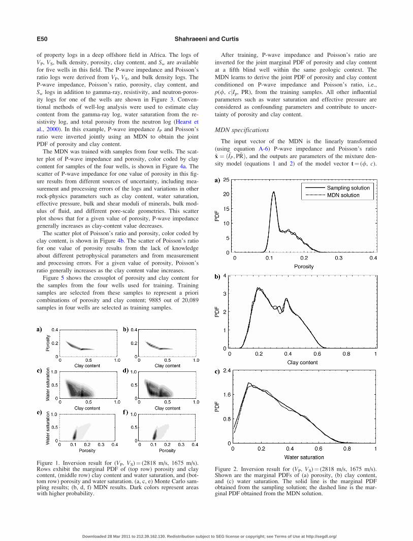
Figure 1 shows the joint a posteriori 2D marginal PDFs of

model parameters evaluated at (VP, VS)¼ (2818 m/s, 1675 m/s).

Figure 1a, c, and e shows the result of Monte Carlo sampling

inversion, and Figure 1b, d, and f shows the result of the diago-

nal MDN inversion. The marginal PDF of porosity, clay content,

and water saturation, obtained from diagonal MDN inversion, is

compared to Monte Carlo sampling inversion results in Figure 2.

The comparison between the results of the Monte Carlo sampling

solution and the diagonal MDN solution in Figures 1 and 2 shows

that the accuracy of the diagonal MDN solution is not perfect as

a result of the finite number of kernels used, but it may be suffi-

ciently good for many applications, particularly given the distinct

computational advantages illustrated below.

In summary, the diagonal MDN can be used to estimate the a

posteriori marginal joint PDF of a subset of model parameters

in a nonlinear inverse problem.

Field example: Inversion of P-wave impedance andPoisson’s ratio logs for porosity and clay content

Forward rock-physics model, a priori PDF of modelparameters, and training data set

In the second application, we apply the diagonal MDN to

obtain the joint PDF of porosity and clay content from samples



of property logs in a deep offshore field in Africa. The logs of

VP, VS, bulk density, porosity, clay content, and Sw are available

for five wells in this field. The P-wave impedance and Poisson’s

ratio logs were derived from VP, VS, and bulk density logs. The

P-wave impedance, Poisson’s ratio, porosity, clay content, and

Sw logs in addition to gamma-ray, resistivity, and neutron-poros-

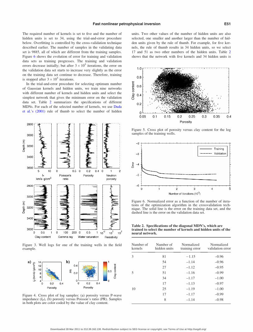
ity logs for one of the wells are shown in Figure 3. Conven-

tional methods of well-log analysis were used to estimate clay

content from the gamma-ray log, water saturation from the re-

sistivity log, and total porosity from the neutron log (Hearst et

al., 2000). In this example, P-wave impedance IP and Poisson’s

ratio were inverted jointly using an MDN to obtain the joint

PDF of porosity and clay content.

The MDN was trained with samples from four wells. The scat-

ter plot of P-wave impedance and porosity, color coded by clay

content for samples of the four wells, is shown in Figure 4a. The

scatter of P-wave impedance for one value of porosity in this fig-

ure results from different sources of uncertainty, including mea-

surement and processing errors of the logs and variations in other

rock-physics parameters such as clay content, water saturation,

effective pressure, bulk and shear moduli of minerals, bulk mod-

ulus of fluid, and different pore-scale geometries. This scatter

plot shows that for a given value of porosity, P-wave impedance

generally increases as clay-content value decreases.

The scatter plot of Poisson’s ratio and porosity, color coded by

clay content, is shown in Figure 4b. The scatter of Poisson’s ratio

for one value of porosity results from the lack of knowledge

about different petrophysical parameters and from measurement

and processing errors. For a given value of porosity, Poisson’s

ratio generally increases as the clay content value increases.

Figure 5 shows the crossplot of porosity and clay content for

the samples from the four wells used for training. Training

samples are selected from these samples to represent a priori

combinations of porosity and clay content; 9885 out of 20,089

samples in four wells are selected as training samples.

After training, P-wave impedance and Poisson’s ratio are

inverted for the joint marginal PDF of porosity and clay content

at a fifth blind well within the same geologic context. The

MDN learns to derive the joint PDF of porosity and clay content

conditioned on P-wave impedance and Poisson’s ratio, i.e.,

p(/, cjIp, PR), from the training samples. All other influential

parameters such as water saturation and effective pressure are

considered as confounding parameters and contribute to uncer-

tainty of porosity and clay content.

MDN specifications

The input vector of the MDN is the linearly transformed

(using equation A-6) P-wave impedance and Poisson’s ratio

~x ¼ ð~IP;P~RÞ, and the outputs are parameters of the mixture den-

sity model (equations 1 and 2) of the model vector t¼ (/, c).

Figure 2. Inversion result for (VP, VS)¼ (2818 m/s, 1675 m/s).Shown are the marginal PDFs of (a) porosity, (b) clay content,and (c) water saturation. The solid line is the marginal PDFobtained from the sampling solution; the dashed line is the mar-ginal PDF obtained from the MDN solution.

Figure 1. Inversion result for (VP, VS)¼ (2818 m/s, 1675 m/s).Rows exhibit the marginal PDF of (top row) porosity and claycontent, (middle row) clay content and water saturation, and (bot-tom row) porosity and water saturation. (a, c, e) Monte Carlo sam-pling results; (b, d, f) MDN results. Dark colors represent areaswith higher probability.



The required number of kernels is set to five and the number of

hidden units is set to 34, using the trial-and-error procedure

below. Overfitting is controlled by the cross-validation technique

described earlier. The number of samples in the validating data

set is 9885, all of which are different from the training samples.

Figure 6 shows the evolution of error for training and validation

data sets as training progresses. The training and validation

errors decrease initially; but after 3� 105 iterations, the error on

the validation data set starts to increase very slightly as the error

on the training data set continue to decrease. Therefore, training

is stopped after 3� 105 iterations.

In the trial-and-error procedure for selecting optimum number

of Gaussian kernels and hidden units, we train nine networks

with different number of kernels and hidden units and select the

simplest network that gives the minimum error on the validation

data set. Table 2 summarizes the specifications of different

MDNs. For each of the selected number of kernels, we use Duda

et al.’s (2001) rule of thumb to select the number of hidden

units. Two other values of the number of hidden units are also

selected, one smaller and another larger than the number of hid-

den units given by the rule of thumb. For example, for five ker-

nels, the rule of thumb results in 34 hidden units, so we select

17 and 51 as two other numbers of the hidden units. Table 2

shows that the network with five kernels and 34 hidden units is

Figure 3. Well logs for one of the training wells in the fieldexample.

Figure 4. Cross plot of log samples: (a) porosity versus P-waveimpedance (IP), (b) porosity versus Poisson’s ratio (PR). Samplesin both plots are color coded by the value of clay content.

Figure 5. Cross plot of porosity versus clay content for the logsamples of the training wells.

Figure 6. Normalized error as a function of the number of itera-tions of the optimization algorithm in the crossvalidation tech-nique. The solid line is the error on the training data set, and thedashed line is the error on the validation data set.

Table 2. Specifications of the diagonal MDN’s, which aretrained to select the number of kernels and hidden units of theneural network.

Number ofkernels

Number ofhidden units

Normalizedtraining error

Normalizedvalidation error

3 81 �1.15 –0.96

54 –1.14 –0.96

27 –1.12 –0.95

5 51 –1.16 –0.99

34 –1.17 –1.00

17 –1.13 –0.97

10 25 –1.19 –1.00

17 –1.17 –0.99

8 –1.14 –0.98



the simplest network that gives the smallest error on the valida-

tion data set.

Inversion results

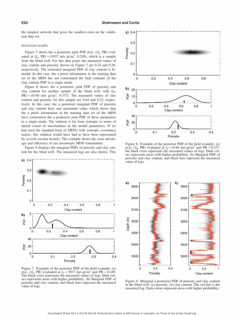
Figure 7 shows the a posteriori joint PDF p(/, cjIp, PR) eval-

uated at (Ip, PR)¼ (5837 m/s g/cm3, 0.249), which is a sample

from the blind well. For this data point, the measured values of

clay content and porosity shown on Figure 7 are 0.24 and 0.28,

respectively. The estimated marginal PDF of clay content is bi-

modal. In this case, the a priori information in the training data

set of the MDN has not constrained the final estimate of the

clay content PDF to a single mode.

Figure 8 shows the a posteriori joint PDF of porosity and

clay content for another sample of the blind well, with (IP,

PR)¼ (6146 m/s g/cm3, 0.337). The measured values of clay

content and porosity for this sample are 0.64 and 0.22, respec-

tively. In this case, the a posteriori marginal PDF of porosity

and clay content have one maximum value, which shows that

the a priori information in the training data set of the MDN

have constrained the a posteriori joint PDF of these parameters

to a single mode. The solution is far from isotropic in terms of

lateral extent of uncertainties in the model parameters. If we

had used the standard form of MDNs with isotropic covariance

matrix, this solution would have had to have been represented

by several circular kernels. The example shows the clear advant-

age and efficiency of our anisotropic MDN formulation.

Figure 9 displays the marginal PDFs of porosity and clay con-

tent for the blind well. The measured logs are also shown. This

Figure 7. Example of the posterior PDF of the field example: (a)p(/, cjIp, PR) evaluated at Ip¼ 5837 m/s�g/cm3 and PR¼ 0.249.The black cross represents the measured values of logs. Dark col-ors represents areas with higher probability. (b) Marginal PDF ofporosity and clay content, and black bars represent the measuredvalue of logs.

Figure 8. Example of the posterior PDF of the field example: (a)p(/, cjIp, PR) evaluated at Ip¼ 6146 m/s�g/cm3 and PR¼ 0.337,the black cross represents the measured values of logs. Dark col-ors represents areas with higher probability. (b) Marginal PDF ofporosity and clay content, and black bars represent the measuredvalue of logs.

Figure 9. Marginal a posteriori PDF of porosity and clay contentin the blind well: (a) porosity, (b) clay content. The red line is themeasured log. Dark colors represent areas with higher probability.



figure shows that the PDFs of porosity and clay content are

good estimates of the measured porosity log.

Figure 10a shows the marginal PDFs of porosity and clay

content in addition to the Sw log for the 3040–3100-m interval

of the blind well. In this interval, Sw varies between zero and

one; the results show that its effect is nevertheless generally

successfully integrated out by the MDN. Figure 10b shows the

marginal PDFs of porosity and clay content for another interval

with variable water saturation. Figures 10a and 10b shows that

variations of Sw do not affect the quality of the MDN estimate

of porosity and clay content logs because the effect of water sat-

uration is integrated out by the MDN.

DISCUSSION

The extension of the MDN to the kernels with variable diago-

nal elements in a covariance matrix results in more accurate

estimates of the joint PDF of the model parameters. To demon-

strate this improvement, we trained four isotropic MDNs (i.e.,

MDNs with a scalar multiple of identity matrix as the covari-

ance matrix [Nabney, 2004]) with the same training data set as

that used in the synthetic application. Table 3 summarizes the

specifications of the different MDNs. The number of hidden

units for all isotropic networks was 10, the same as the diagonal

network. As Table 3 shows, the best training error achieved by

the isotropic MDNs is 20% larger than the diagonal MDN. For

the isotropic MDN with 21 kernels, the number of weights and

biases is equal to the number of weights and biases of the diag-

onal MDN. Table 3 displays that in this case the training error

of the isotropic MDN is about 23% larger than the error of the

diagonal MDN.

Figure 11 shows the result of the diagonal MDN in addition

to the result of the isotropic MDN with 21 kernels. Clearly, the

inversion result obtained by the isotropic MDN is less accurate

than the result of the diagonal MDN. Figure 11a, c, and e shows

that the uncertainty of the joint PDFs of porosity and clay con-

tent, clay content, and Sw, and porosity and Sw, obtained using

isotropic MDN is larger than diagonal MDN, which is a better

estimate of the Monte Carlo sampling solution (Figure 1). Thus,

applying the diagonal MDN results in better approximations of

multidimensional PDFs than applying the isotropic MDN.

The diagonal Gaussian kernels, however, are less flexible than

Gaussian kernels with a full covariance matrix. Applying full

covariance matrices with an MDN is computationally more

Figure 10. Marginal a posteriori PDF of porosity and clay contentfor two intervals with variable water saturation: (a) 3040–3100-minterval, (b) 3450–3490-m interval. Darker colors show the areaswith high probability, and the red line is the measured log.

Table 3. Specifications of the diagonal and isotropic MDN’sused to solve the synthetic problem.

NetworkNumber of

Gaussian kernels

Number ofweights and biases

of the networkNormalized

error

Diagonal 15 1185 �1

Isotropic 1 15 855 �0.74

Isotropic 2 18 1020 �0.76

Isotropic 3 21 1185 �0.77

Isotropic 4 23 1350 �0.79

Figure 11. Comparison between results of the MDN inversionusing isotropic Gaussian kernels and diagonal Gaussian kernels.Inversion result for (VP, VS)¼ (2818 m/s, 1675 m/s). First row isthe joint marginal PDF of porosity and clay content: (a) isotropicMDN result, (b) diagonal MDN result. Second row is the jointmarginal PDF of clay content and water saturation: (c) isotropicMDN result, (d) diagonal MDN result. Third row is the joint mar-ginal PDF of porosity and water saturation: (e) isotropic MDNresult, (f) diagonal MDN result. Dark colors represent areas withhigher probability.



complex than applying diagonal covariance matrices because we

need to derive an analytical representation of the derivatives of

the error function (equation A-3) with respect to the elements of

the inverse of the covariance matrix—the same as those derived

for the diagonal covariance matrix (equations 6, 7, and 8). What

is more, to estimate valid values of the diagonal elements of

the covariance matrix, we need to represent these parameters

as positive functions of the network outputs (equation 4). With

a full covariance matrix, this problem is more complicated be-

cause the covariance matrix and its inverse should be symmetric

and positive definite (Williams, 1996). Therefore, we need to

parameterize the positive definite matrices in such a way that

(1) the parameters can freely assume any real values (because

the outputs of neural network can assume any real value), (2)

the determinant is a simple expression of the parameters, and

(3) the correspondence is bijective. Williams (1996) develops

such a parameterization and applies it to build an MDN with a

single Gaussian kernel with full covariance matrix. However,

because of the increase in the number of the outputs of the neu-

ral network, extension of that method to cases with more than

one kernel is computationally expensive and can destabilize the

network during training.

The synthetic application shows that the diagonal MDN solu-

tion of a nonlinear inverse problem is a good estimate of the

Monte Carlo sampling solution. The main advantage of the di-

agonal MDN is its speed. A single training iteration took 65.37

s, and the total training time for this network was around 240

hours on a standard personal computer. After training, each fully

nonlinear probabilistic inversion took 915 ms. Therefore, if we

use this network for inversion, in 48 hours it will provide the

full posterior PDF of the model vector for 188,850,000 data

points. Calculating the Monte Carlo sampling solution by for-

ward modeling of 500,000 samples took around 625 s; in the

same total time as the MDN training and inversion (i.e., 288

hours), the grid-search method will invert only 1700 data points.

Obviously, the relative advantage of the MDN increases with

the number of inverse problems to be solved because training

time becomes a smaller portion of the total inversion time (e.g.,

in 1000 hours, the MDN solves 2.99 billion problems but the

grid search method solves only 5800 problems). This is of great

utility when inverting massive data sets point by point (e.g.,

logs from many wells or 3D seismic cubes that typically might

contain 109 data points).

The second advantage of the diagonal MDN method is its

memory efficiency. Each fully probabilistic MDN inversion

result can be stored by the parameters of the mixture-density

model. The number of such parameters depends on the number

of kernels and the dimensionality of the model space; typically

it might be on the order of tens or hundreds in the kind of appli-

cations discussed here. However, the Monte Carlo sampling so-

lution of one problem typically requires saving thousands of

accepted samples to represent the solution.

These two advantages are obtained at the expense of accuracy

of the estimated PDF. For some cases, the error in estimating

the PDF can be large. For example, because of the smoothness

of Gaussians, the error in estimating a truly uniform PDF (with

abrupt variations in the PDF at the boundaries of the unit inter-

val) with Gaussian kernels can be high. The accuracy of the

estimate can be improved if the number of kernels is increased

or if more flexible kernels such as Gaussians with a full instead

of a diagonal covariance matrix are used. However, both of

these possible improvements require estimating more kernel pa-

rameters, which is more time consuming. The computing cost of

MDN training increases as the number of network parameters or

training samples increases. Therefore, solving inverse problems

with very high-dimensional model and data space can be com-

putationally demanding unless very large computer facilities are

available.

Another drawback of using MDN to solve inverse problems

is the trial-and-error procedure for selecting the appropriate

number of hidden units and kernels. This procedure can be very

slow, depending on the number of training samples.

The Gaussian mixture model (equation 1) has been used in

different applications to model arbitrary PDFs. Ghahramani

(1993) and Grana and Della Rossa (2010) apply the Gaussian

mixture model to solve inverse problems using sampling techni-

ques. In this approach, samples of model vector m and data

vector d are used to estimate the joint PDF of model and data

vector p(m,d) using a Gaussian mixture model. Then for a given

value of data d¼ d0, the conditional PDF of m given data d0, or

p(mjd0), is obtained using the Gaussian mixture model of

p(m,d). The so-called expectation-maximization algorithm,

which is computationally efficient, is usually used to estimate

the Gaussian mixture model of an arbitrary PDF from a set of

samples. The number of required samples to represent p(m,d)

properly increases exponentially as the dimension of model and

data spaces increase (Bishop, 1995). In such cases, the number

of required kernels in the Gaussian mixture model can be very

large, and the speed of the convergence of the expectation-maxi-

mization algorithm decreases significantly (Grana and Della

Rossa, 2010). However, because of the interpolation ability of

neural networks, the MDN approach requires fewer training

samples and can be more appropriate in cases with high-dimen-

sional model and data spaces. Also, the number of required

kernels in an MDN is significantly fewer than the number

of kernels in the Gaussian mixture model because the MDN

approximates p(mjd0) for given values of d0, whereas the Gaus-

sian mixture model approximates p(m,d) for all possible values

of d.

The field example shows that the MDN can be used to obtain

rock properties (i.e., porosity and clay content) from seismic-at-

tribute logs (i.e., P-wave impedance and Poisson’s ratio) without

applying an independent petrophysical forward function. In this

case with a limited number of training samples, the proper

design and training procedure of the MDN is more important

than cases with a possibly unlimited number of training samples

(e.g., synthetic example) because of the higher chance of over-

fitting. The result of such completely data-driven applications of

the MDN is acceptable only if they are tested against data that

are not used in the training procedure. The results of the inver-

sion in this application are acceptable in a blind well. Thus, the

geologic setting and relations between acoustic properties and

rock properties in the blind well are nearly the same as other

wells used in the training procedure.

The a posteriori uncertainty of the estimated parameters might

be decreased if, for example, spatial information about the dis-

tribution of rock properties at the wellbore was used. Such in-

formation might be included in the training data set by defining

model and data vectors for a group of neighboring samples

(Caers and Ma, 2002) instead of for each individual sample as



used in this paper. However, because of computer memory

requirements for defining such model and data vectors, we have

not tested this possibility.

In our example, we invert P-wave impedance and Poisson’s ra-

tio for porosity and clay content. Another parameter of interest in

petrophysical inversion is Sw. To invert for water saturation, we

need to use a theoretical forward function to generate synthetic

data to model water-saturated sandy intervals (in our case study,

all water-saturated training data samples were shaly). The applica-

tion of a theoretical forward function will reduce the uncertainty

in model parameters by adding theoretical information about the

relation between the model and data vectors. Gassmann’s law can

be used for fluid substitution to produce synthetic data that repre-

sent all possible values of water saturation. We only used the

well-log data for inversion and did not address the problem of

theoretical forward model selection and calibration. Nevertheless,

this did not pose any limitation on the method as presented,

which can in principle be used to invert any forward petrophysi-

cal relationship, whether analytic, synthetic, or data driven.

CONCLUSIONS

A diagonal MDN can be trained to provide a fully probabilis-

tic solution to a nonlinear, Bayesian inverse problem. The diag-

onal MDN solution of many similar inverse problems can be

much faster to compute than the corresponding sampling-based

solution, yet the diagonal MDN provides a good estimate of the

sampling solution. The accuracy of the diagonal MDN can be

improved by using more kernels or by increasing the flexibility

of the kernels. However, these improvements can significantly

increase the required time for training and inversion.

We have applied the diagonal MDN to invert P-wave imped-

ance and Poisson’s ratio for the joint PDF of porosity and clay

content in a real field example. We show that if the diagonal MDN

is designed and trained properly, the estimated a posteriori PDFs

of the model parameters are good representations of the measured

log values. The estimated a posteriori PDF represents the uncer-

tainty of uncontrolled factors — most importantly, perhaps, Sw.

Our synthetic example indicates that Sw and its associated uncer-

tainty can also be estimated.

ACKNOWLEDGMENTS

We thank TOTAL E&P UK for sponsoring this work, researchers

and staff at the Geoscience research center for their help, and Christian

Deplante, Gabriel Chao, and Olivier Dubrule in particular for their val-

uable and positive feedback and discussions. We acknowledge the

support from the Scottish Funding Council for the joint research insti-

tute with the Heriot-Watt University, which is part of Edinburgh

Research Partnership in Engineering and Mathematics (ERPem).

APPENDIX A

TWO-LAYER FEED-FORWARD

NEURAL NETWORKS

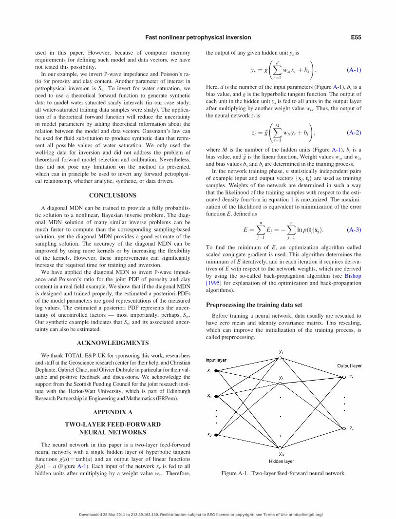
The neural network in this paper is a two-layer feed-forward

neural network with a single hidden layer of hyperbolic tangent

functions g(a)¼ tanh(a) and an output layer of linear functions

~gðaÞ ¼ a (Figure A-1). Each input of the network xr is fed to all

hidden units after multiplying by a weight value wsr. Therefore,

the output of any given hidden unit ys is

ys ¼ gXd

r¼1

wsrxr þ bs

!: (A-1)

Here, d is the number of the input parameters (Figure A-1), bs is a

bias value, and g is the hyperbolic tangent function. The output of

each unit in the hidden unit ys is fed to all units in the output layer

after multiplying by another weight value wts. Thus, the output of

the neural network zt is

zt ¼ ~gXM

s¼1

wtsys þ bt

!; (A-2)

where M is the number of the hidden units (Figure A-1), bt is a

bias value, and ~g is the linear function. Weight values wsr and wts

and bias values bs and bt are determined in the training process.

In the network training phase, n statistically independent pairs

of example input and output vectors {xj, tj} are used as training

samples. Weights of the network are determined in such a way

that the likelihood of the training samples with respect to the esti-

mated density function in equation 1 is maximized. The maximi-

zation of the likelihood is equivalent to minimization of the error

function E, defined as

E ¼Xn

j¼1

Ej ¼ �Xn

j¼1

ln pðtjjxjÞ: (A-3)

To find the minimum of E, an optimization algorithm called

scaled conjugate gradient is used. This algorithm determines the

minimum of E iteratively, and in each iteration it requires deriva-

tives of E with respect to the network weights, which are derived

by using the so-called back-propagation algorithm (see Bishop

[1995] for explanation of the optimization and back-propagation

algorithms).

Preprocessing the training data set

Before training a neural network, data usually are rescaled to

have zero mean and identity covariance matrix. This rescaling,

which can improve the initialization of the training process, is

called preprocessing.

Figure A-1. Two-layer feed-forward neural network.



Here, we use the whitening preprocessing algorithm. Whitening

is a linear transformation of data used to whiten the input vector

of the MDN x ¼ x1;…; xdð ÞT , i.e., transform it to a new data set

with zero mean and identity covariance matrix. Consider a train-

ing data set {xj, tj} with n statistically independent samples. The

sample mean vector �x and covariance matrix R of the input vec-

tors xj is given by

�x ¼ 1

n

Xn

j¼1

xj; (A-4)

R ¼ 1

n� 1

Xn�1

j¼1

xj � �x� �

xj � �x� �T

: (A-5)

The whitened input vector ~xj is then given by

~xj ¼ �K�1=2UT xj � �x� �

: (A-6)

The value K is the eigenvalue matrix, and U is the eigenvector

matrix of the covariance matrix R. The transformed input data ~xj

have zero mean and unit covariance matrix (Fukunga, 1990).

APPENDIX B

FORWARD PETROPHYSICAL MODEL

FOR THE SYNTHETIC PROBLEM

Dvorkin and Gutierrez (2001) propose the following forward

rock-physics model for a dispersed sand-clay mixture. The forward

model is defined for two classes of facies: (1) sands and shaly sands

and (2) shales and sandy shales. For sands and shaly sands, a sand

matrix with porosity /s is assumed; clay particles are dispersed in

the pore space between sand grains and cause a decrease in poros-

ity. Therefore, as the clay content increases, the pore space fills

with stiffer material and the bulk and shear moduli increase. When

the amount of clay exceeds the pure sand porosity /s, the sand ma-

trix starts to collapse and clay particles fill the contact between sand

grains, resulting in a softer rock. Therefore, for clay-content values

larger than /s, the bulk and shear moduli decrease as clay content

increases. This behavior is modeled mathematically as

c < /s : / ¼ /s � cð1� /cÞ; (B-1)

c � /s : / ¼ c/c: (B-2)

In equations B-1 and B-2, / is the porosity of the mixture, /c is

the porosity of pure shale, /s is the porosity of pure sand, and c is

the clay content.

The bulk modulus Kmix and shear modulus Gmix of shales and

sandy shales are modeled by the lower Hashin-Shtrikman bound

(Mavko et al., 2009):

c � /s;Kmix ¼c

K2 þ 4G2

3

þ 1� c

Ks þ 4 G2

3

" #�1

� 4

3G2; (B-3)

Gmix ¼c

G2 þ Z2

þ 1� c

Gs þ Z2

� ��1

� Z2;

Z2 ¼G2

6

9K2 þ 8G2

K2 þ 2G2

:

(B-4)

In the equations B-3 and B-4, K2 and G2 are the bulk and shear

moduli of fluid saturated pure shale matrix, respectively, derived

as from equations B-14 and B-15, and Ks and Gs are the bulk and

shear moduli of sand particles.

The bulk and shear moduli of the sands and sandy shales are

also modeled by the lower Hashin-Shtrikman bound:

c < /s;Kmix ¼

c

/sand

� �K1 þ 4 G1

3

þ1� c

/sand

� �Kcc þ 4G1

3

2664

3775�1

� 4

3G1;

(B-5)

Gmix ¼

c

/sand

G1 þ Z1

þ1� c

/sand

Gcc þ Z1

264

375�1

� Z1;

Z1 ¼G1

6

9K1 þ 8G1

K1 þ 2G1

:

(B-6)

In equations B-5 and B-6, K1 and G1 are the bulk and shear mod-

uli of pure sand matrix, respectively, derived from equations B-14

and B-15; Kcc and Gcc are given by Kmix and Gmix as derived from

equations B-3 and B-4 for c¼/s.

The elastic properties of the pure dry sand and pure dry shale

matrices are given by the Hertz-Mindlin theory (Mavko et al.,

2009) as

Ki dry ¼ni

2ð1� /iÞ2li

18p2ð1� miÞ2P

" #1=3

; (B-7)

li dry ¼5� 4mi

5 ð2� miÞ3 ni

2 ð1� /iÞ2 li

2 p2ð1� miÞ2P

" #1=3

: (B-8)

In equations B-7 and B-8, i is an index that can be s for a pure

sand matrix and c for a pure shale matrix; P is the effective pres-

sure; li and vi are the shear modulus and Poisson’s ratio of the

grain materials (i.e., sand particles for sands and clay particles for

shale), respectively; and ni is the coordination number (the aver-

age number of contacts per grain), approximated by the empirical

equation (Mavko et al., 2009)

ni ¼ 20� 34 /i þ 14 /2i : (B-9)

Effective pressure is a function of depth; it is given by

P ¼ g

ðz0

ðqb � qf Þ dz; (B-10)

where qb is bulk density, qf is fluid density, z is depth, and g is

gravitational gravity. According to Batzle and Wang (1992), the

bulk modulus and density of any type of hydrocarbon (with a

given value of density at standard conditions) are empirical func-

tions of pore pressure and temperature. In equation B-10, if we

assume that pore pressure and overburden stress are hydrostatic,

then the effective pressure will also be hydrostatic. Therefore, the

empirical relation between bulk modulus (or density) of fluid and

pore pressure is transformed into a relation between bulk modulus

(or density) of fluid and effective pressure.



Porosity of the pure sand and clay matrix is a decreasing func-

tion of depth as a result of the compaction effect (Avseth et al.,

2005). The relationship between porosity and depth is usually

approximated by an exponential function:

/i ¼ /i0 expð�cizÞ; (B-11)

where /i0 is the depositional porosity (or critical porosity) of sand

or shale and ci is a constant that varies for sand and shale

deposits.

The density of the fluid-saturated rock qmix is given as

c < /s : qmix ¼ ð1�/sÞqsþ cð1�/cÞqcþ/qf ; (B-12)

c� /s : qmix ¼ ð1� cÞqsþ cð1�/cÞqc þ/qf ; (B-13)

where qs, qc, and qf are the density of sand particles, clay par-

ticles, and fluid, respectively.

The bulk and shear modulus of the fluid-saturated pure sand

and fluid saturated pure shale matrices are given by Gassmann’s

law as

Kj ¼ Ki

Ki dry

Ki � Ki dry

þ Kf

/iðKi � Kf Þ

1þ Ki dry

Ki � Ki dry

þ Kf

/iðKi � Kf Þ

; (B-14)

Gj ¼ Gi dry; (B-15)

where j is equal to one for fluid-saturated pure sand matrix, with iequal to s. For fluid-saturated pure shale, matrix j is equal to two

and i is equal to c. The values Ki_dry and Gi_dry are the bulk and

shear moduli of the dry frame matrices of sand and shale and are

derived from equations B-7 and B-8.

The fluid bulk modulus and density Kf and qf are functions of

fluid saturation. For a mixture of brine and oil, if we assume the

pore fluid is uniformly distributed in the pores, these parameters

are given as

Kf ¼Sw

Kwþ 1� Sw

Khc

� ��1

; (B-16)

qf ¼ Swqw þ ð1� SwÞqhc; (B-17)

where Kw and qw are the bulk modulus and density of brine and

Khc and qhc are the bulk modulus and density of oil. The bulk

moduli and densities of brine and oil are functions of effective

pressure.

The compressional- and shear-wave velocities of the dispersed

sand and shale mixture are given by

VP ¼

ffiffiffiffiffiffiffiffiffiffiffiffiffiffiffiffiffiffiffiffiffiffiffiKmix þ 4Gmix

3

qmix

s; (B-18)

VS ¼ffiffiffiffiffiffiffiffiffiGmix

qmix

s; (B-19)

where Kmix, Gmix, and qmix are obtained from equations B-3–B-6,

B-12, and B-13 depending on the value of clay content. Equations

B-18 and B-19 imply that the mixture of sand and shale is iso-

tropic and elastic.

In our synthetic example, we assume the depositional porosity

of sand /s0 is equal to 0.45, the depositional porosity of shale is

equal to 0.60, the compaction factor of sand cs is equal to

0.127 km�1, the compaction factor of shale cc is equal to 0.45

km�1, the bulk modulus of brine Kw is 2.80 GPa, and the density

of brine is 1.09 g/cm3. The effective pressure is assumed to be

hydrostatic pressure, given by P¼ (qmix � qf)gz. The density,

gravity, and gas-oil ratio of oil, required to estimate the density

and bulk modulus of oil as a function of pore pressure (and

hence effective pressure) at standard conditions, are 0.78 g/cm3,

32 API, and 64 Sm3/Sm3. These data are from Avseth et al.

(2005). Shale is not a granular composite such as sand. There-

fore, the validity of applying equations B-7, B-8, and B-14 to

pure shale is not obvious. However, there is evidence that these

equations provide reasonable elastic-property estimates (Avseth

et al., 2005). We do not promote applying those equations for

pure shale, and we applied them in the synthetic case to show

that the MDN inversion method can solve inverse problems with

high-dimensional model space.

REFERENCES

Avseth, P., T. Mukerji, A. Jorstad, G. Mavko, and T. Veggeland, 2001,Seismic reservoir mapping from 3-D AVO in a North Sea turbidite sys-tem: Geophysics, 66, 1157–1176, doi:10.1190/1.1487063.

Avseth, P., T., Mukerji, and G. Mavko, 2005, Quantitative seismic inter-pretation: Cambridge University Press.

Bachrach, R., 2006, Joint estimation of porosity and saturation using sto-chastic rock-physics modeling: Geophysics, 71, no. 5, O53–O63,doi:10.1190/1.2235991.

Batzle, M., and Z., Wang, 1992, Seismic properties of pore fluids: Geo-physics, 57, 1396–1408, doi:10.1190/1.1443207.

Bishop, C., 1994, Mixture density networks: Neural Computing ResearchGroup Technical Report NCRG/94/004, Aston University.

——, 1995, Neural networks for pattern recognition: Oxford UniversityPress.

Caers, J., and X. Ma, 2002, Modeling conditional distributions of faciesfrom seismic using neural nets: Mathematical Geology, 34, no. 2, 143–167, doi:10.1023/A:1014460101588.

Chen, J., and Y., Rubin, 2003, An effective Bayesian model for lithofaciesestimation using geophysical data: Water Resources Research, 39,SBH4–1–SBH4–11.

Devilee, R., A. Curtis, and K. Roy-Chowdhury, 1999, An efficient, proba-bilistic neural network approach to solving inverse problems: Invertingsurface wave velocities for Eurasian crustal thickness: Journal of Geo-physical Research, 104, no. B12, 28841–28856, doi:10.1029/1999JB900273.

Dubrule, O., 2003, Geostatistics for seismic data integration in earthmodels: SEG.

Duda, R., P. Hart, and D. Stork, 2001, Pattern classification: Wiley Inter-science.

Dvorkin, J., and M. A. Gutierrez, 2001, Textural sorting effect on elasticvelocities, Part II: Elasticity of a bimodal grain mixture: 71st AnnualInternational Meeting, SEG, Expanded Abstracts, 1764–1767, doi:10.1190/1.1816466.

Eidsvik, J., P. Avseth, H. Omre, T. Mukerji, and G. Mavko, 2004, Stochas-tic reservoir characterization using prestack seismic data: Geophysics,69, 978–993, doi:10.1190/1.1778241.

Fukunga, K., 1990, Introduction to statistical pattern recognition: Aca-demic Press.

Ghahramani, Z., 1993, Solving inverse problems using an EM approach todensity estimation: Proceedings of the 1993 Connectionist ModelsSummer School, 316–323.

Grana, D., and E. Della Rossa, 2010, Probabilistic petrophysical-properties estimation integrating statistical rock physics withseismic inversion: Geophysics, 75, no. 3, O21–O37, doi:10.1190/1.3386676.

Hearst, J. R., P. H. Nelson, and F. L. Paillet, 2000, Well logging for physi-cal properties: A handbook for geophysicists, geologists, and engineers,2nd ed.: John Wiley & Sons Ltd.

Maiti, S., and R. K. Tiwari, 2009, A hybrid Monte Carlo method based ar-tificial neural networks approach for rock boundaries identification: Acase study from the KTB bore hole: Pure and Applied Geophysics, 166,2059–2090, doi:10.1007/s00024-009-0533-y.



——, 2010, Automatic discriminations among geophysical signals via theBayesian neural networks approach: Geophysics, 75, no. 1, E67–E78,doi:10.1190/1.3298501.

Maiti, S., R. K. Tiwari, and H. J. Kumpel, 2007, Neural network modelingand classification of lithofacies using well log data: A case study fromKTB borehole site: Geophysical Journal International, 169, 733–746,doi:10.1111/j.1365-246X.2007.03342.x.

Mavko, M., T. Mukerji, and J. Dvorkin, 2009, The rock physics handbook:Cambridge University Press.

McLachlan, G., and D. Peel, 2000, Finite mixture models: WileyInterscience.

Meier, U., A. Curtis, and J. Trampert, 2007a, Global crustal thicknessfrom neural network inversion of surface wave data: Geophysical Jour-nal International, 169, 706–722, doi:10.1111/j.1365-246X.2007.03373.x.

——, 2007b, A global crustal model constrained by nonlinearised inver-sion of fundamental mode surface waves: Geophysical Research Let-ters, 34, L16304, doi:10.1029/2007GL030989.

Meier, U., J. Trampert, and A. Curtis, 2009, Global variations of tempera-ture and water content in the mantle transition zone from higher mode

surface waves: Earth and Planetary Science Letters, 282, no. 1–4, 91–101, doi:10.1016/j.epsl.2009.03.004.

Nabney, I., 2004, NETLAB: Algorithms for pattern recognition: Springer-Verlag.

Poulton, M., 2002, Neural networks as an intelligence amplification tool: Areview of applications: Geophysics, 67, 979–993, doi:10.1190/1.1484539.

Roth, G., and A. Tarantola, 1994, Neural networks and inversion of seis-mic data: Journal of Geophysical Research, 99, no. B4, 6753–6768,doi:10.1029/93JB01563.

Saggaf, M. M., M. N. Toksoz, and H. M. Mustafa, 2003, Estimation of res-ervoir properties from seismic data by smooth neural networks: Geo-physics, 68, 1969–1983, doi:10.1190/1.1635051.

Spikes, K., T. Mukerji, J. Dvorkin, and G. Mavko, 2007, Probabilistic seis-mic inversion based on rock-physics models: Geophysics, 72, no. 5,R87–R97, doi:10.1190/1.2760162.

Tarantola, A., 2005, Inverse problem theory and methods for model pa-rameter estimation: SIAM.

Williams, P. M., 1996, Using neural networks to model conditional multi-variate densities: Neural Computation, 8, 843–854, doi:10.1162/neco.1996.8.4.843.



fast probabilistic nonlinear petrophysical inversion...fast probabilistic nonlinear petrophysical...

Documents