Fair Pricing of Energy DerivativesA Comparative Study

Mahmoud Hamada�

Energy Risk Management - EnergyAustralia

May 7, 2004

Abstract

The Australian National Electricity Market (NEM) is a highly volatilemarket in which price setting is driven by the law of supply and demand.The volatile nature of this market presents signi�cant risk to market par-ticipants and as such stabilisation of price has implications for the pre-vention of �nancial distress.

To alleviate the risk associated with this volatility, over the counter -and eventually exchange traded - derivatives allow hedge positions to beestablished, thus resulting in a less volatile hedged exposure to the under-lying. With the importance of derivative trading for market participants,consistent methods of derivative pricing become important.

This paper is a comparative study of two existing quantitative ap-proaches for pricing energy derivatives, namely: a cash-�ow at risk modelbased on Monte Carlo simulation of the underlying spot price, combinedwith extreme value theory, and the SDE approach based on no-arbitragetheory utilising convenience yields and cost of carry to address the inabil-ity to store electricity.

The paper provides a presentation of the underlying theory of the twoapproaches with an empirical comparative study, contrasting calibrationmethods to quoted brokerage premiums and statistical methods of estima-tion from historical data. Advantages and disadvantages of both methodsare discussed in light of the results obtained.

1 Motivation and Objectives

De�ning the fair value of derivatives is not a simple task. In insurance, a fairvalue of a contingent claim is calculated by taking expectations of the claimpayo¤ with addition of the claim variance or standard deviation to account forrisk. In some other cases, when utility functions are used, the fair value isde�ned to be the certainty equivalent of the claim. The certainty equivalent is

�The author acknowledges support from Peter Murray and Tim O�grady. Discussion withPhil Moody was very useful and empirical work of Brett Gray is greatly appreciated.

1

the amount which, when received by certainty, is regarded as good as taking therisk. In �nancial markets, the fair value of an option is the expectation of thediscounted payo¤, where the expectation is taken under a di¤erent probabilitymeasure. When the underlying risk is assumed to be log-normally distributed,Black-Scholes like formulae for options can be obtained. It should be stressedthat, in capital markets, many ad-hoc methods were used before the Black andScholes methodology gained the consensus among di¤erent market participants.And even though it is widely used, it is well known that its assumptions are notrealistic and it cannot be applied to pricing all types of options.With the liberalisation of the Australian electricity industry, electricity prices

are determined through a process of supply and demand and as such are �oatingin nature. The underlying spot price of NSW electricity has been observed tobe highly volatile and at times of high demand, extreme price events occur rep-resenting a signi�cant risk to market participants. As such, market participantshave the need to hedge the risk associated with the volatile nature of the un-derlying and this is done through the trade of derivative contracts as similar tothose found in the more typical capital markets. Such derivative trading couldbe considered to have indirect e¤ects relating to the continuity of supply andthe stability of the industry. If any market participant was to enter �nancialdistress due to unhedged exposure, supply could potentially be a¤ected.With the importance of derivative trading there arises the need to determine

appropriate derivative pricing techniques that are suitable to the structure ofthis market and existing methods adopted in the capital markets should beexplored for this purpose. Among di¤erent alternatives, two approaches standout:

� The cash �ow at risk approach, based on historical price distribution. Anoption price is computed by taking the di¤erence payments evaluated ateach path of the Monte Carlo simulation and then computing a quantileto re�ect the price that the market is trading at.

� The Stochastic Di¤erential Equations (SDE) approach where the underly-ing dynamics are modeled via mean-reverting di¤usion process, and thenclosed form solutions -akin Black and Scholes- for option prices can beobtained

Both approaches are genuine and have their strengths and weaknesses. Theaim of this paper is to explore, and compare these two methodologies fromtheoretical and empirical aspects.Furthermore, with the proposal for Australian electricity participants to

adopt the IAS 39 international accounting standard currently adopted inter-nationally (see http:// www.iasplus.com/standard/ias39.htm), consistent valu-ation of energy derivatives is required here. The standard includes two possiblemethods for determining electricity derivative premia, an approach based onthe assessment of market quotes and the other based on discounted cash-�owanalysis. In studying the two methods above, we explore each of these options,

2

adopting the SDE approach to calibrate to quoted premia and the cash-�ow atrisk approach as the basis for the discounted cash-�ow analysis.The paper is organised as the following. Section two details the idea and the

mathematics behind the cash�ow at risk based on historical price distribution.It explains the long range dependence concept and its use in the ARIMAX timeseries model. Then it explores a way to model spikes in historical prices usingextreme value theory and Hill (1975) estimation.Section three considers the SDE approach. It presents two di¤erent models

known as Schwartz single and two factor models. Closed-from solutions to optionprices are given in this framework as well as the risk sensitivities to underlyingmarket parameters ("Greeks") for the one factor model.Section four provides a comparison between the two approaches where cali-

bration to broker cap premia methodology is explained and discussion of resultsis given.

2 Cash�ow at Risk Based on Historical PriceDistribution

This section details the cash �ow at risk methodology adopted and is intendedas a more intuitive account of the process.It is well known in the literature and from empirical investigation that elec-

tricity spot prices exhibit cycles, seasonality and autocorrelation. This datastructure can be captured and used to forecast future spot prices. We alsoknow that occasional price spikes may occur due to unusual high load, networktransmission constraints and unscheduled outages of generation. These extremevalues and their probability of occurrence can also be captured from historicaldata and used in the Monte Carlo simulation.In �nancial markets, Monte Carlo methods are recognised as very �exible

tools for simulating future time series with which to evaluate cost and risk of var-ious contracts. Possible future values can be generated by randomly samplingthe relevant distributions, maintaining given volatility characteristics. MonteCarlo methods are relatively well understood, and can model correlations. Addi-tionally such methods can achieve better accuracy by using complex dependencyon the path taken to date.The cash�ow at risk methodology adopted in this paper is based on a

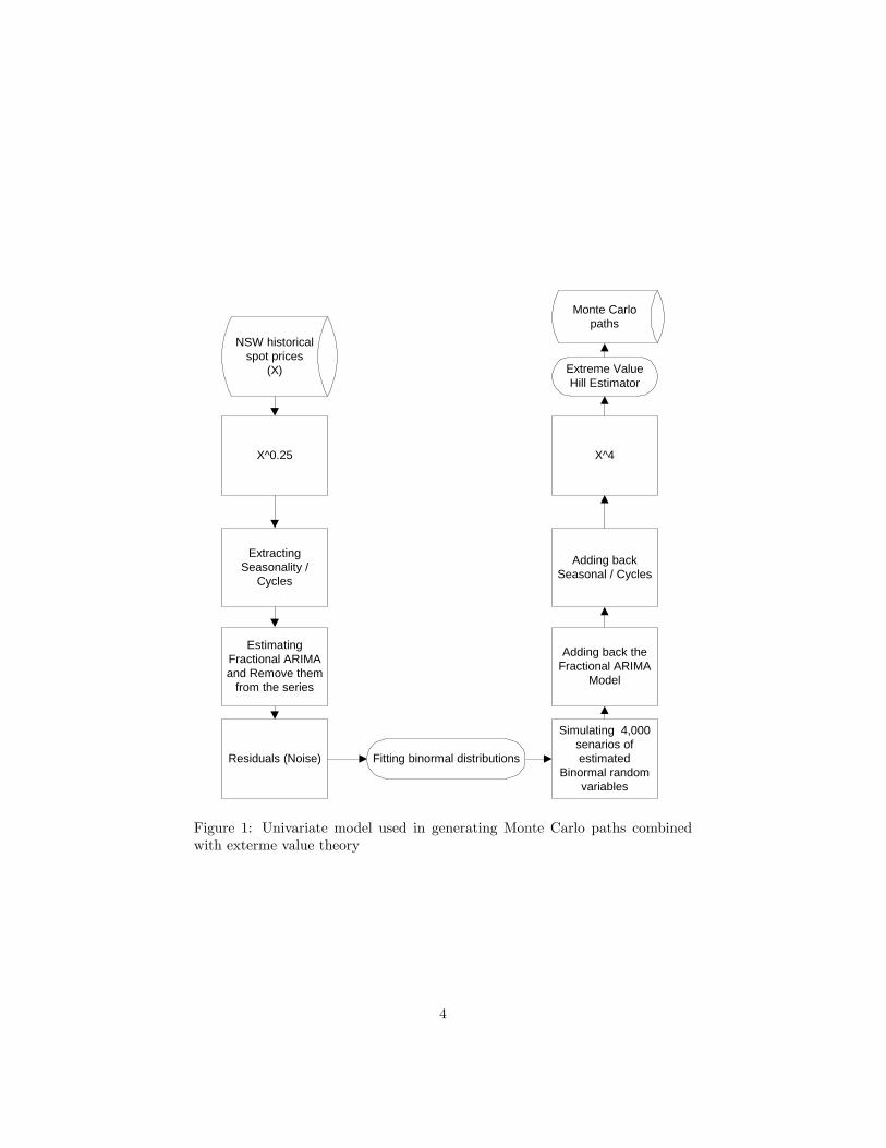
methodology originally developed at Katestone Analytic and is based on atime series analysis approach. The methodology uses Mote Carlo simulationin which future simulated paths retain the cyclic and seasonal e¤ects of historicspot as well as the autocorrelation structure and extreme price events typicallyobserved.The approach initially involves the development of a time series model of the

underlying, which is to be estimated from historical data. Figure (1) illustratessuch a model. Initially the historical data is raised to the power of 0.25 (afourth root). This has the e¤ect of dampening the extreme occurrences observed

3

X^0.25

ExtractingSeasonality /

Cycles

EstimatingFractional ARIMAand Remove them

from the series

Simulating 4,000senarios ofestimated

Binormal randomvariables

Adding back theFractional ARIMA

Model

Adding backSeasonal / Cycles

X^4

Residuals (Noise) Fitting binormal distributions

Extreme ValueHill Estimator

NSW historicalspot prices

(X)

Monte Carlopaths

Figure 1: Univariate model used in generating Monte Carlo paths combinedwith exterme value theory

4

historically and makes the data more able to be analysed by other time seriesmethods. Following this, the daily, weekly and yearly cyclic e¤ects present in thehistorical data are estimated. This allows the seasonal and peak/o¤-peak e¤ectsin the underlying series to be represented mathematically in a manner in whicha Monte-Carlo method can incorporate these cyclic e¤ects into the simulationprocess. Once this structure is estimated, it is removed from the historic dataso that the series remaining is a representation of the historic underlying (toforth root) that has been deseasonalised and had peak/o¤-peak e¤ects removed.A key feature of the simulation of sample paths for electricity market vari-

ables is the maintenance of observed serial correlation structure in the series.The fractional ARIMA time-series methodology is used to estimate and removethe temporal correlations and long memory from such variables. After thisprocess, the �nal residuals of the analysis, after the removal of the cyclic andthe fractional ARIMA estimation should represent values that are uncorrelatedin time and have close to bi-normal distributions.In order to generate a simulated path, the simulation process proceeds by

repeated sampling from distributions estimated from the residuals of the aboveanalysis, followed by a reconstruction of the full time-series by adding the es-timated fractional ARIMA structure and cyclic information and inverting theforth root operation initially adopted.The distribution estimated from the �nal residuals is �tted to a mixture

of Normal distributions and allows the proper treatment of longer, fatter tailsin price distributions due to the physical constraints of the electricity market.Following the construction of such a simulated path, the Hill estimator is usedto estimate the jump size and frequency from historical data and incorporatethe extreme price events often observed in this industry.Having generated a large number of representative price paths, the expected

contract payouts for a given portfolio can be evaluated. Option prices and cash-�ow at risk measures can then be evaluated from averages or higher quantilesand distributional parameters evaluated over the family of possible time series.Exotic options are readily treated by the standard decomposition into a linearcombination of contract legs, where legs can be either cap, �oor, swap or binaryoptions.

2.1 Historical Prices Structure

2.1.1 Long Range Dependence

Karen Lunney (1995) observes: "Most environmental data can be describedqualitatively as having long serial correlations in the time domain, �icker noise inthe frequency domain and space �lling capacity of the graphical representationsof the data, also called fractal characteristics. Another common characteristiccan be described as intermittency which can be de�ned as sudden bursts of highfrequency behaviour".Processes exhibiting these characteristics may have long range dependence.

It is not surprising that we observe similar characteristics in electricity prices

5

Figure 2: Time Plot of the Logarithm of Spot Prices since 1999

Figure 3: Fast Fourrier Trasform of Spot Prices

6

Figure 4: Autocorrelation of half-hourly spot prices

data; see �gures (2), (3) and (4). This is because electricity prices mainlydepend, among other factors, on electricity demand, which itself depends onweather conditions. Many studies show that environmental measurement (suchas rainfall, temperature, humidity, ozone concentrations, ...) have long tem-poral and spacial correlations. In order to better understand the idea of longrange dependence, the �eld of critical phenomena is an area where long rangedependence has physical interpretation. For example, a liquid may be in equilib-rium with neighbouring molecules and the correlation relationship may be onlyweakly dependent. As the liquid approaches a critical temperature, however,where a phase transition to the gaseous phase occurs, the dependence structurechanges with molecular correlation decaying very slowly, that is, long rangedependence.In the following section we present fractional ARIMA time series model

which allows to capture the long range dependence.

2.1.2 Di¤erencing and Standard ARIMA Models

The idea behind ARIMA Stationary models are an important class ofstochastic models. This class of models assumes that the process remains inequilibrium about a constant mean level. Much development has been doneto study the properties of such models. Now, if the process is non-stationary,-exhibiting explosive behaviour- it can be possible in some cases to transform itto a stationary process in order to use existing tools to study its properties, thenbacking out the non-stationary model parameters. The Autoregressive Moving

7

Average models are an example of stationary time series.ARIMA time series model, developed by Box and Jenkins are an extension

to the ARMA models using di¤erencing1 . This method allows for the series tobe di¤erenced if necessary in order to obtain stationarity, and then the resultingseries may be treated as an ordinary ARMA model. The I stands for the wordintegrating meaning summing, the inverse of the di¤erencing operation. So,integrating an ARIMA process will yield an ARMA process.

Mathematical development We will now present a formulation of theARIMAmodel based on Box et.al. (1994). A sequence fztgt�1 is said to be governedby the autoregressive moving average model ARMA(p; q) of orders p and q if itsatis�es the following equation

zt = ('1zt�1 + :::+ 'pzt�p) + (�0et + �1et�1 + �2et�2 + :::+ �qet�q)

where ('i) and(�j) with 1 � i � p and 1 � j � q are constants and fetgt�1is white noise. If we de�ne the the lag operator B by Bxt = xt�1; hence,Bmxt = xt�m, for any integer m; then the above equation can be written as

(1� '1B � :::� 'pBp)zt = (�0 + �1B + �2B2 + :::+ �qBq)et

or'(B)zt = �(B)et (1)

where '(B) and �(B) are polynomials in the lag operator B, of degrees p andq, respectively. An ARMA process is stationary if all the roots of '(B) = 0 lieoutside the unit circle2 , and is non-stationary if some of the roots lie inside theunit circle.The third case which happens to be interesting is that for which the roots

of '(B) = 0 lie on the unit circle. It turns out that the resulting models are ofgreat value in representing non-stationary time series.Suppose that d of the roots of '(B) = 0 are unity and the remainder lie

outside the unit circle. Then the model (1) can be expressed in the form

�(B)(1�B)dzt = �(B)et (2)

where �(B) is stationary autoregressive operator. If we denote the di¤erencingoperator O; such that Oxt = xt � xt�1 = (1�B)xt; then the model (2) can bere-written as

�(B)wt = �(B)et (3)

and wt = Odzt (4)

1Di¤erencing a time series is transforming it to another time series where each element isthe di¤erence between two consecutive elements of the original time series

2 if B� is the solution to '(B) = 0 then jB�j > 1

8

Thus we see that the model corresponds to assuming that the dth di¤erence ofthe series can be represented by a stationary ARMA process.For d � 1; the process z can be deduced from equation (4) to give

zt = Sdwt (5)

where S is the in�nite summation operator de�ned by

Sxt =1

1�Bxt

= (1 +B +B2 +B3 + ::::)xt

Equation (5) implies that the process (2) can be obtained by summing or"integrating" the stationary process (3) d times. Hence the name autoregressiveintegrated moving average (ARIMA) process.Now, the parameter d need not be integer. Indeed, it is always possible to

to write1

(1�B)d= �0 + �1B + �2B

2 + :::

for example1

(1�B)0:5= 1 +

1

2B +

3

8B2 +

5

16B3 + :::

In the case when 0 � d � 1; the model is called fractional ARIMA. In section(2.1.3), we present an algorithm for estimating d from the data.

2.1.3 Fractional ARIMA Models

The standard ARIMA models as presented in the previous section use an in-teger di¤erencing parameter. However, this parameter can be any real numberbetween 0 and 1, given the argument at the end of the previous section. In thiscase, they are called fractional ARIMA models.In the previous section we analysed the properties of ARMA models in the

time domain, that is the properties of fztgt�1 where t represents time. Anequivalent analysis of the time series can be performed in the frequency domain.

The idea behind going back to frequency domain An alternative way ofanalysing a time series is to assume that it is made up of sine and cosine waveswith di¤erent frequencies. A device that uses this idea is the periodogram.Suppose that the number of observations in the time series, N = 2q + 1 is odd.We can �t the Fourier series model

zt = �0 +

qXi=1

(�icit + �isit) + et

where cit = cos(2�fit); sit = sin(2�fit); and fi = iN is the ith harmonic of the

fundamental frequency 1N ; the least squares estimates of the coe¢ cients �0 and

9

(�i; �i) will be b�0 = z

b�i =2

N

NXt=1

ztcit

b�i =2

N

NXt=1

ztsit

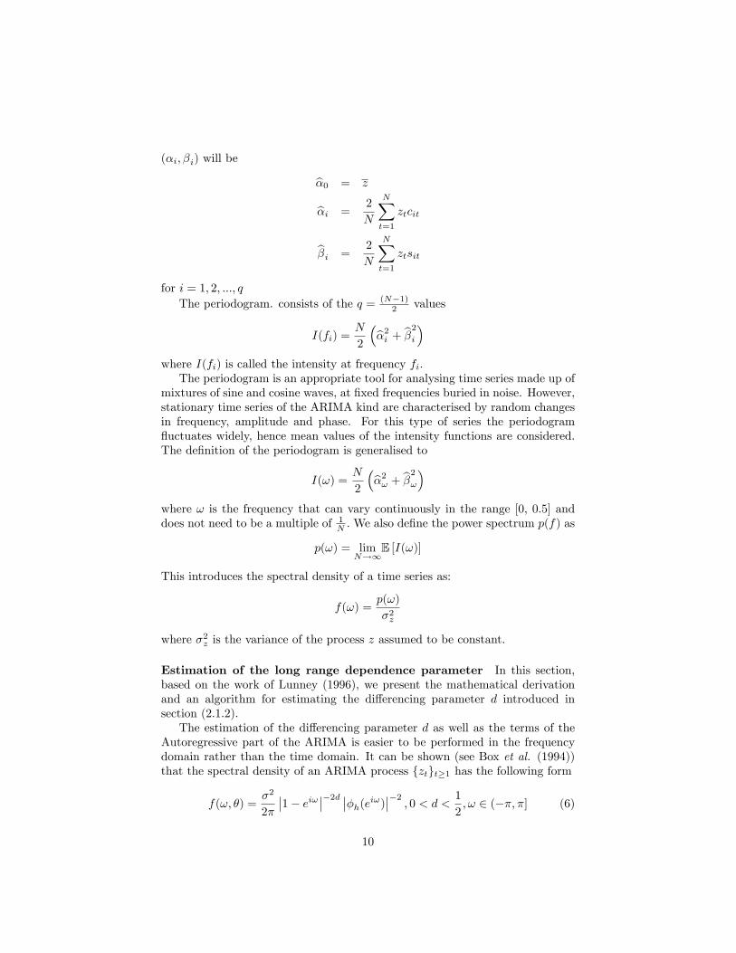
for i = 1; 2; :::; qThe periodogram. consists of the q = (N�1)

2 values

I(fi) =N

2

�b�2i + b�2i�where I(fi) is called the intensity at frequency fi:The periodogram is an appropriate tool for analysing time series made up of

mixtures of sine and cosine waves, at �xed frequencies buried in noise. However,stationary time series of the ARIMA kind are characterised by random changesin frequency, amplitude and phase. For this type of series the periodogram�uctuates widely, hence mean values of the intensity functions are considered.The de�nition of the periodogram is generalised to

I(!) =N

2

�b�2! + b�2!�where ! is the frequency that can vary continuously in the range [0; 0:5] anddoes not need to be a multiple of 1

N :We also de�ne the power spectrum p(f) as

p(!) = limN!1

E [I(!)]

This introduces the spectral density of a time series as:

f(!) =p(!)

�2z

where �2z is the variance of the process z assumed to be constant.

Estimation of the long range dependence parameter In this section,based on the work of Lunney (1996), we present the mathematical derivationand an algorithm for estimating the di¤erencing parameter d introduced insection (2.1.2).The estimation of the di¤erencing parameter d as well as the terms of the

Autoregressive part of the ARIMA is easier to be performed in the frequencydomain rather than the time domain. It can be shown (see Box et al. (1994))that the spectral density of an ARIMA process fztgt�1 has the following form

f(!; �) =�2

2�

��1� ei!���2d ���h(ei!)���2 ; 0 < d < 1

2; ! 2 (��; �] (6)

10

where � 2 �, the vector of all parameters on the right hand side of equation (6),and � is a compact subset of Rn, n being the number of elements of �, and

�h(ei!) = 1� �1ei! � �2ei2! � :::� �heih!

with �h(z) 6= 0 for jzj < 1. The factor��1� ei!���2d in (6) corresponds to dth

order di¤erencing.The estimation of the vector of parameters � can be obtained by minimising

min�

Z �

��

�log f(!; �) +

IT (!)

f(!; �)

�d! (7)

where IT (!) is the unbiased periodogram based on the sample fz1; :::; zT g. Thisyields the asymptotic maximum likelihood estimator of �. It can be shown fromLunney (1995) that problem (7) is equivalent to

min�

Z �

��

�IT (!)

f�(!)

�d!

where

f�(!) =��1� ei!���2d ����h(ei!)����2

Let us de�neIT (!)

f�(!)= �T (!) (8)

We have E[�T (!)] = 1 since IT (!) is unbiased estimator of f�(!). Also, asshown by Yajima (1989), f�T (!j)g is an asymptotically independent sequenceunder some conditions which are satis�ed by model (6) here for the Fourierfrequencies. Equation (8) yields

log IT (!) = log f�(!) + log �T (!)

At the Fourier frequencies, this equation becomes

logIT (!j)

�h(!j)= �d log

�2 sin

!j2

�2+ log �T (!j) (9)

Now, we can estimate the di¤erencing parameter d using least squares ap-plied to the regression (9), so that

bd = �P0<!j<�=3log

IT (!j)�h(!j)

log�2 sin

!j2

�2P

0<!j<�=3

�log�2 sin

!j2

�2�2 (10)

Yet to be estimated the unknown parameters of �h. So we re-write equation(9) as

log IT (!j) = log �h(0)� d log�2 sin

!j2

�2+ log

�h(!j)

�h(0)+ log �T (!j) (11)

11

At low frequencies, i.e. ! is near zero, the term log �h(!j)�h(0)is negligible relative

to the other terms on the right hand side of (11). Therefore, d can roughly beestimated by applying least squares to the regression (11). This estimated valueof d is an approximation that will be considered as an an initial value of d:Now, the order and parameters of �h can now be estimated by taking the

Discrete Fourier Transfer (DFT) of

Is(!j) =�2 sin

!j2

�2bd0IT (!j)

This will yield estimates of the covariance function of wt = (1� B)dzt. AnAR(h) model can now be �tted to these covariances using the Durbin-Levinsonrecursion. BIC can be used to select the model order, where

BIC = log �2h;d + hlog T

T

�2h;d being the minimum prediction error variance for the data given d and h.Now, given h, the parameters �j , j = 1; :::; h; of �h can be estimated usingmaximum likelihood.At this step, given the estimated values of h and parameters, �i, we can use

equation (10) to compute an unbiased estimator for d. This estimator can inturn be used in the AR �tting step to gain better estimates for h and �i. Thisprocedure can be iterated until convergence to accurate values of d, h and �j ,j = 1; :::; h is obtained.

2.2 Extreme Values Estimation

The normal distribution has a normal tail, which means that values beyondthree standard deviation have less than 0:27% of occurrence. In order to modelelectricity prices where extreme values have higher probability of occurrence,fat tail distributions should be considered. There are families of distributionswhich have this property, such as elliptical distributions and extreme value dis-tributions, i.e. Gumbel, Fréchet or Weibull (see Kotz and Nadarajah 2000).Once an extreme value distribution is chosen, some of its parameters indicatethe fatness of the tail.The Hill estimator essentially looks at the data and estimates the fatness

parameter so that the resulting distribution has the appropriate shape.

2.2.1 Mathematical development

As pointed earlier, electricity prices are heavy-tailed. One of the issues in thestudy of long-tailed probability distributions is the estimation of the tail index�, which measure the heaviness the tail of the distribution. Let X1; X2; :::; Xnbe an independent and identically distributed random sample from a long-taileddistribution F such that, for su¢ ciently large x; the distribution F is assumedto have the algebraic functional form. That is, 1 � F (x) � Cx�� for x � D;

12

where � is the (upper) tail index, D is the threshold above which the assumedalgebraic from is valid, and C is a normalising constant. De�ne X(1) � X(2) �::: � X(n) as the descending order statistics from the distribution F: A tail indexestimator derived from maximum likelihood considerations and known as theHill estimator (Hill 1975), is de�ned as

�(r)H =

r + 1Pri=1 i ln

�x(i)

x(i+1)

� ;where r + 1 is the number of observations above the threshold D: The imple-mentation of the Hill estimator, however, requires a choice of the number ofextreme order statistics, r; from a sample of size n; where 2 < r + 1 � n; orequivalently the threshold D:There are methods which allow estimation of the threshold D from data (see

Hsieh 1999). In our analysis, we take D as an input. Indicative values for peakseason D = $100 and for o¤-peak D = $70:Section (4) below presents simulations using the above cash-�ow at risk

methodology and compares results to the SDE approach detailed below.

3 Stochastic Di¤erential Equation Approach

The SDE approach is another paradigm in modelling electricity prices. It hasthe advantage of representing the dynamics of the underlying forward or spotprices with a stochastic di¤erential equation and using the stochastic calculusin deriving closed form solutions to option prices written on this underlying. Inmany electricity markets a mean-reverting and jump-di¤usion process is popu-larly used in modelling the electricity spot price; see for example Deng (2000),Johnson and Barz (1999) and Clewlow, Strickland and Kaminski (2001). Nev-ertheless, there are two important challenges in pricing electricity derivatives.The �rst challenge is accurate parameters estimation of the mean-reverting jumpdi¤usion stochastic process. The second is to derive a pricing measure underwhich option prices equal the mean of discounted payo¤s.It is clear that the more factors the model has, the more characteristics of

electricity it can capture, i.e. mean reversion, seasonal e¤ects, price dependentvolatility, occasional price spikes... However, this means more parameters tocalibrate.Given the lack of liquidity in the electricity market, the calibration of multi-

factor models is not stable. Let us consider the one and two factor models tostudy the stability of the calibration and the consistency of pricing. We baseour presentation of the models on Clewlow and Strickland (2000).

3.1 One Factor Model

The single factor model introduced by Schwartz (1997) assumes that the spotprice follows a mean-reverting stochastic process.

13

dStSt

= � [�� ln(St)] dt+ �dWt (12)

where � is the mean reversion rate (the speed of adjustment of the spot priceback towards its long term level �) and � is the spot price volatility. Assuminga constant short term interest rate over the period [t; T ]; European call optionprice is given by:

c(t;K; T ) = e�r(T�t)�F (t; T )N(h)�KN(h�

pw)�

where

h =

ln

�F (t; T )

K

�+ 1

2w

pw

; w =�2

2�

h1� e�2�(T�t)

iN(�) is the standard normal cumulative distribution function, and

F (t; T ) = exp

�e��(T�t) ln(St) +

�1� e��(T�t)

���� �2

2�

�+�2

4�

�1� e�2�(T�t)

��Here r is the continuously compounded short term interest rate. This modelneeds three parameters to be calibrated. We shall detail the calibration exercisein section 3.4. It is worth noting that one does not need to implement thedynamics of the underlying as given in equation (12) in order to price optionson this underlying. The closed form of the call option c(t;K; T ) is readilycomputed without simulation.

3.2 Two Factor Model:

3.2.1 Convenience yield

The convenience yield measures the advantage of holding the commodity minusthe cost of storage. In electricity markets, plants seek to minimise their cost ofproduction by avoiding the cost of shutting down and restarting the plant dueto high prices or lack of available supplies. Hence the concept of convenienceyield can be applicable when the source of electricity is fuel or coal.

3.2.2 The model

Although simple to implement, the one factor model has very simple volatilitystructure which goes to zero with increasing maturities. Schwartz (1997) in-troduce a two factor model where the �rst factor is the underlying spot priceand the second factor is the convenience yield. The �rst factor is the spot pricewhich is assumed to follow a di¤usion process

dSt = (r � �t)Stdt+ �StdWt

where r is the short term interest rate and �t is the convenience yield at time t,� is spot price volatility and W is the Brownian motion.

14

The second factor is the instantaneous convenience yield of spot energy andhas the following mean-reverting process:

d�t = ��(� � �t)dt+ ��dZt

where �� and � represent the speed of adjustment and long term mean of theconvenience yield, �� is the convenience yield volatility and Zt is the Brownianmotion. The two Brownian motions used in the spot price and the convenienceyield dynamics, Wt and Zt are correlated with correlation coe¢ cient �S�; i.e.dWtdZt = �S�dt:The forward energy prices can be derived (Schwartz (1997))

F (t; s) = St exp

���t

1� e���(s�t)��

+A(t; s)

�where

A(t; s) =

�r � � + 1

2

�2��2�� ����S�

��

�(s� t) + 1

4�2�1� e�2��(s�t)

�3�+�

��� + ����S� ��2���

�1� e���(s�t)

�2�

The price of a European call option, maturing at time T; with strike priceK on the spot price is given by:

c(t;K; T ) = e�r(T�t)�F (t; T )N(h)�KN(h�

pw)�

where

h =ln [F (t; T )=K] + 1

2wpw

w = �2(T � t)� 2����S���

(T � t)�

�1� e���(T�t)

���

!+

�2��2�

�(T � t)� 2

��

�1� e���(T�t)

�+

1

2��

�1� e�2��(T�t)

��

3.3 Pricing Caps

Energy price caps limit the �oating price of energy the holder will pay on apredetermined set of dates T + i�T ; i = 1; :::; N to a �xed cap level K. A cap istherefore a portfolio of standard European call options with its price given by

CAP (t;K; T;N;�T ) =NXi=1

c(t;K; T + i�T )

15

3.4 Calibration

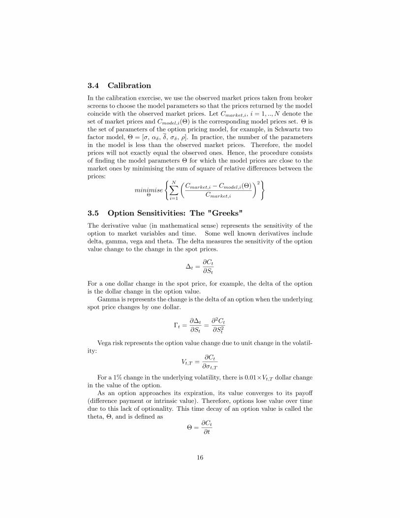
In the calibration exercise, we use the observed market prices taken from brokerscreens to choose the model parameters so that the prices returned by the modelcoincide with the observed market prices. Let Cmarket;i, i = 1; ::; N denote theset of market prices and Cmodel;i(�) is the corresponding model prices set. � isthe set of parameters of the option pricing model, for example, in Schwartz twofactor model, � = [�; ��; �; ��; �]. In practice, the number of the parametersin the model is less than the observed market prices. Therefore, the modelprices will not exactly equal the observed ones. Hence, the procedure consistsof �nding the model parameters � for which the model prices are close to themarket ones by minimising the sum of square of relative di¤erences between theprices:

minimise�

(NXi=1

�Cmarket;i � Cmodel;i(�)

Cmarket;i

�2)

3.5 Option Sensitivities: The "Greeks"

The derivative value (in mathematical sense) represents the sensitivity of theoption to market variables and time. Some well known derivatives includedelta, gamma, vega and theta. The delta measures the sensitivity of the optionvalue change to the change in the spot prices.

�t =@Ct@St

For a one dollar change in the spot price, for example, the delta of the optionis the dollar change in the option value.Gamma is represents the change is the delta of an option when the underlying

spot price changes by one dollar.

�t =@�t@St

=@2Ct@S2t

Vega risk represents the option value change due to unit change in the volatil-ity:

Vt;T =@Ct@�t;T

For a 1% change in the underlying volatility, there is 0:01�Vt;T dollar changein the value of the option.As an option approaches its expiration, its value converges to its payo¤

(di¤erence payment or intrinsic value). Therefore, options lose value over timedue to this lack of optionality. This time decay of an option value is called thetheta, �; and is de�ned as

� =@Ct@t

16

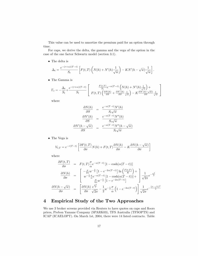
This value can be used to amortize the premium paid for an option throughtime.For caps, we derive the delta, the gamma and the vega of the option in the

case of the one factor Schwartz model (section 3.1).

� The delta is

�t =e�(r+�)(T�t)

St

�F (t; T )

�N(h) +N 0(h)

1pw

��KN 0(h�

pw)

1pw

�:

� The Gamma is

�t = ��tSt+e�(r+�)(T�t)

St

24 F (t;T )St

e��(T�t)�N(h) +N 0(h) 1p

w

�+

F (t; T )�@N(h)@S + @N 0(h)

@S1pw

��K @N 0(h�

pw)

@S1pw

35where

@N(h)

@S=

e��(T�t)N 0(h)

Stpw

@N 0(h)

@S=

e��(T�t)N 00(h)

Stpw

@N 0(h�pw)

@S=

e��(T�t)N 00(h�pw)

Stpw

� The Vega is

Vt;T = e�r(T�t)

�@F (t; T )

@�N(h) + F (t; T )

@N(h)

@��K@N(h�

pw)

@�

�where

@F (t; T )

@�= F (t; T )

�

�e��(T�t) [1� cosh(�(T � t))]

@N(h)

@�=

264 � �2�w

� 32

�1� e�2�(T�t)

�ln�F (t;T )K

�+

w�12��e

��(T�t) [1� cosh(�(T � t))]+�4�w

� 12

�1� e�2�(T�t)

�375 1p

2�e�

h2

2

@N(h�pw)

@�=

"@N(h)

@�

eh2

2

p2�� 12w�

12�

�

�1� e�2�(T�t)

�# 1p2�e�

(h�pw)2

2

4 Empirical Study of the Two Approaches

We use 3 broker screens provided via Reuters to have quotes on caps and �oorsprices, Prebon Yamane Company (SPARK03), TFS Australia (TFSOPTS) andICAP (ICAELOPT). On March 1st, 2004, there were 14 listed contracts. Table

17

Contract Market Premium Cash�ow at Single Factor Two Factor

$/MWH Risk $/MWH $/MWH $/MWH

NSW Q204 FLAT CAP 300 7.88 10.74 3.49 1.35NSW APR-DEC 04 OFF PEAK CAP 300 2.35 3.85 3.39 3.22NSW APR-DEC 04 FLAT CAP 300 6.25 4.68 3.39 3.26NSW APR-DEC 04 FLAT CAP 100 6.80 5.86 8.39 4.88NSW Q304 FLAT CAP 300 8.00 7.11 3.41 3.85NSW FIN 04/05 FLAT CAP 300 7.63 3.93 3.28 4.04NSW FIN 04/05 FLAT CAP 100 8.13 5.09 8.03 5.04NSW Q404 FLAT CAP 300 2.75 1.17 3.28 4.56NSW Q105 PEAK CAP 300 28.50 5.26 3.23 4.22NSW Q105 FLAT CAP 300 12.50 4.12 3.23 4.22NSW Q105 FLAT CAP 100 13.50 5.94 7.92 4.85NSW CAL 05 FLAT CAP 300 7.58 3.79 3.18 3.18NSW CAL 05 FLAT CAP 100 8.38 4.95 7.80 3.49NSW CAL 05 OFF PEAK CAP 300 2.18 3.31 3.18 3.19

Table 1: Market vs. model implied premiums of brokered contracts

(1) presents the broker quotes with the valuations of the three models overthe same set of contracts while table (2) presents absolute percentage errorsof valuations and MAPEs (Mean Absolute Percentage Errors) for each of themodels. We will now proceed to discuss these results in terms for each of thethree models tested.

4.1 Cash �ow at Risk Monte-Carlo Methodology

The cash �ow at risk Monte-Carlo model was estimated with historical pooldata from 1/1/1999 �1/3/2004. A simulation was then run, generating 4000simulated paths of future spot price and these paths were used to calculate thepro�t distribution of the di¤erence payments incurred by holding each of thebroker contracts. A model implied contract premium was then determined byadopting a given quantile (percentile) of the pro�t distribution and consideringthat quantile to be the premium (converted to a $/MWH �gure). The selectionof the appropriate quantile to adopt provides an indication of the risk premiuminherent in the contracts�premia. The quantile at a probability of 0.5 (i.e. the50th percentile) could be considered a contract value in which no risk premiumis present. As the quantile moves further up the pro�t distribution, the riskpremium can be considered larger.In order to determine the appropriate quantile of the pro�t distributions

to adopt, the quantile�s probability was optimised to the observed option pre-mia such that the objective function presented in section (3.4) was minimised.The quantile�s probability as optimised over the entire set of broker contracts,was the largest 0.99075 (i.e. the 99.075th percentile) of the pro�t distribution.

18

Contract Name Cash�ow at Risk Single Factor Two Factor

NSW Q204 FLAT CAP 300 36.34 55.70 82.82NSW APR-DEC 04 OFF PEAK CAP 300 63.96 44.21 37.16NSW APR-DEC 04 FLAT CAP 300 25.06 45.70 47.84NSW APR-DEC 04 FLAT CAP 100 13.85 23.34 28.21NSW Q304 FLAT CAP 300 11.14 57.31 51.92NSW FIN 04/05 FLAT CAP 300 48.42 56.97 46.96NSW FIN 04/05 FLAT CAP 100 37.38 1.19 37.98NSW Q404 FLAT CAP 300 57.31 19.21 65.83NSW Q105 PEAK CAP 300 81.53 88.66 85.20NSW Q105 FLAT CAP 300 67.03 74.15 66.20NSW Q105 FLAT CAP 100 55.99 41.35 64.06NSW CAL 05 FLAT CAP 300 49.94 57.99 57.96NSW CAL 05 FLAT CAP 100 40.90 6.90 58.28NSW CAL 05 OFF PEAK CAP 300 52.00 46.32 46.56Mean Absolute Percentage Error 45.77 44.21 55.50

Table 2: Absolute percentage error in model valuations and MAPE for each ofthe three models

This is implying an excessively large risk premium. Essentially the interpreta-tion of this probability is that holding such a cap would only provide di¤erencepayments in excess of the contract�s premium in 0.925% of cases. While thislevel of risk premium appears excessive, it can be explained by the methodologyadopted of replicating historical price structure. As detailed above, the modelfor the underlying is estimated from historical data such that the paths gener-ated would display similar structural and distributional properties to historicalspot price. Table (3) shows the option premia quotes for �at $300 caps of thedi¤erent quarters and the di¤erence payment that would result from holdingsuch caps in history (i.e. the $/MWH di¤erence payment of a $300 cap of therelevant quarter observed historically from 1/1/1999 �1/3/2004). As can beseen from this �gure, current broker quotes are signi�cantly higher than theobserved historical di¤erence payment and as such, this data consistent withthe calibrated model�s risk premium when the assumption is adopted that themodel volatility is estimated from historical data. Table (3) indicates that fora distribution of spot estimated from historical data, the quoted premia wouldbe a high quantile of the contracts cost distribution implied by the model of theunderlying.Such a large observed risk premium would most likely be due to a market

expectation that future volatility may be signi�cantly higher than that observedhistorically as well as the potentially large losses that can occur from sold capin a scenario of high volatility. In the SDE approach, as tested in this paper,the SDE representing the underlying process is calibrated to the quoted optionpremia. A potential bene�t of the SDE approach in contrast to the cash �ow atrisk approach tested here is that higher expectations of future market volatility

19

Contract Quoted Option Di¤erence Payment

Premium ($/MWH) Observed Historically ($/MWH)

NSW Q204 FLAT CAP 300 7.88 6.73NSW Q304 FLAT CAP 300 8.00 3.84NSW Q404 FLAT CAP 300 2.75 1.19NSW Q105 FLAT CAP 300 12.50 3.94

Table 3: Option premium versus historic di¤erence payment measured overhistorical spot data from 1999

Contract Subset Pro�t Quantile ProbabilityAll contracts 0.99075$100 Strike Caps 0.99975$300 Strike Caps 0.97975Peak Caps 0.94650O¤Peak Caps 0.91000Flat Caps 0.99750

Table 4: Calibrated quantile probability of the pro�t distribution when opti-mised on di¤erent subsets of the broker contracts. The degree above 0.5 is anindication of the risk premia for the contracts

can be quanti�ed from quoted market premia. As such, the market premia willto some degree provide an indication of the expectation of the future underlyingprocess. An elaboration of this point is discussed below.This methodology can be used to determine risk premia by di¤erent classi-

�cations of the instruments. Table (4) shows optimised quantile probability ofthe pro�t distributions when calibrated to di¤erent subsets of the broker quotedcontracts.As would be expected, the risk premium for $100 caps is greater than that

for the $300 caps. Additionally, the risk premium for Peak caps is higher thanfor o¤-peak caps. Surprisingly, the premium on �at caps is higher than thatfor peak or o¤-peak. This result may be due however to the speci�c durationof peak and o¤-peak caps in the data set and the lack of liquidity for thesecontracts.The risk premia observed in table (4) provide some insight into the pricing

results observed in table (1). As the pricing in table (1) is based on the quantileprobability optimised with all contracts, the comparatively low risk premiumon the o¤-peak caps means the model has overpriced these caps. The $100 capsand the majority of the �at caps have been underpriced due to the higher riskpremium here.An important property to study for such a model is the stability of model

implied prices over time. As such, the model was used to value the same setof contracts with an additional two days historical spot data. The model wasre-estimated with the extra data, paths were regenerated and the same pro�tdistribution quantile probability was adopted as calibrated from the initial esti-

20

Contract Cash�ow at Risk Cash�ow at Risk Percentage change

$/MWH 1/1/03 $/MWH 3/1/04 in contract value

NSW Q204 FLAT CAP 300 10.74 11.069 3.09NSW APR-DEC 04 OFF PEAK CAP 300 3.85 3.969 3.01NSW APR-DEC 04 FLAT CAP 300 4.68 4.814 2.78NSW APR-DEC 04 FLAT CAP 100 5.86 5.97 1.91NSW Q304 FLAT CAP 300 7.11 7.262 2.15NSW FIN 04/05 FLAT CAP 300 3.93 3.879 -1.37NSW FIN 04/05 FLAT CAP 100 5.09 5.036 -1.02NSW Q404 FLAT CAP 300 1.17 1.026 -12.61NSW Q105 PEAK CAP 300 5.26 5.222 -0.80NSW Q105 FLAT CAP 300 4.12 4.295 4.22NSW Q105 FLAT CAP 100 5.94 6.097 2.61NSW CAL 05 FLAT CAP 300 3.79 3.799 0.18NSW CAL 05 FLAT CAP 100 4.95 4.941 -0.18NSW CAL 05 OFF PEAK CAP 300 3.31 3.362 1.69

Table 5: Cash�ow at risk model valuation of contracts on the 1/1/2004 and the3/1/2004

mation (i.e. 0.99075). Over such a short duration, if the methodology is robustfor pricing, in the absence of major news entering the market a large di¤erencein contract pricing should not be observed. Table (5) shows the original optionprices from the model and the prices determined in the estimation includingthe additional two days data. As can be seen the percentage change in price isnot prohibitive for the use of such a model. The larger change observed for theQ404 Flat $300 Cap is due to its small valuation, as a result of the lack of ex-treme prices typically observed in quarter four. The contributing factors to theobserved price changes include an e¤ect of the di¤erent valuation dates on thepresent valuing of the pro�t distribution and an e¤ect from the additional twodays estimation data. Due to the time di¤erential between the two valuations,we believe these e¤ects would be negligible. As such the primary reason forthe observed percentage change in contract values would be a lack of completeconvergence to the theoretically implied pro�t distribution. Such an e¤ect couldbe remedied through the generation of more paths or the incorporation of moree¢ cient monte-Carlo random number generation techniques such as antitheticvariables and pseudo-random numbers (see Putney 1999).

4.2 Stochastic Di¤erential Equation Approach Results

The single factor model achieved the most accurate calibration to the brokerdata of all the models tested. The additional accuracy over the cash �ow atrisk model may be due to its process of calibrating all model parameters to thebroker data rather than basing its estimation on historical spot data. This hasthe potential bene�t that a model of the underlying is essentially determined

21

via a market consensus through the quoted premia, however issues of a lack ofliquidity in the market may present di¢ culties in such a calibration over othertime frames.Inspection of the prices presented in table (1) illustrates the primary weak-

nesses of the model in relation to the dynamics of the NSW electricity priceunderlying. The model in its current form is unable to account for peak/o¤-peak or seasonally e¤ects. This is evident in the SDE of the underlying processpresented in section (3.1). The model has a constant mean reversion rate, meanreversion level and volatility. As such, the dynamics of the process representedby the SDE will make no distinction based on time of day or time of year. Thisis evident in the displayed model premia. Contracts that have the same strikeprice and time frame are valued with very similar premia for peak, o¤-peak or�at periods. This is contrary to the broker quotes and the general understandingof market participants.The lack of seasonality in the model can be observed in contracts valuations

such as the Q304 $300 Flat Cap and the Q404 $300 Flat Cap. The SDE hasvalued these contracts with almost the same premium, however, the empiricaldata re�ect the fact that Q3 contains a lot of winter volatility while Q4 is acomparatively �at quarter.Due to these factors, further work to adopt an SDE approach should extend

the form presented in section (3.1) to allow such peak/o¤-peak and seasonalitye¤ects and in the representation of the underlying. One way to incorporate suche¤ects would be through the incorporation of a time-dependent volatility termsuch presented below:

dStSt= � [�� ln(St)]dt+ �(t)dWt

The function �(t) should be in a continuous functional form that allows someform of cyclic volatility function through the time of day and months of the year.A higher volatility during peak times of the day and months of the year wouldnaturally provide the required di¤erentiation in option prices and account forthe higher prices observed in the underlying during these periods. A sinusoidalfunctional form with frequencies calibrated to seasonal e¤ects and time of theday can be considered.A further addition to provide a more realistic model of the underlying would

be to include jump di¤usion terms in the process to model extreme price events.While there was not a wide range of cap strike prices present in the broker data,the incorporation of jump di¤usion would be expected to improve the robustnessof valuing contracts over a wider range of strike prices.The calibrated parameters for the single factor model are as follows:

� � �8.25 4.58 6.43

(13)

These parameters can be understood when considering the e¤ect of the lackof jump di¤usion. The value of � represents an electricity price mean reverting

22

level of $97.51. While this is signi�cantly greater than the mean reverting levelof electricity spot price, the model has adopted this to compensate for the lackof a representation of extreme price occurrences in the model of the underlying.One potential strength of such an approach where parameters are calibrated tomarket data is that parameters will be determined such that reasonable inter-polation of contract prices is obtained, even if the dynamics of the underlyingare quite di¤erent from those of the SDE.The parameters determined for the two-factor model are as follows:

� �� � �� �3.66 5.54 1.27 0.05 -0.4

Out of the three models, the two-factor model displayed the worst perfor-mance in calibrating to the broker data. This may imply a lack of signi�canceof the convenience yield concept for this industry. It is well recognised thatextreme price occurrences in the electricity market are typically due to extremeweather conditions causing excessive load. In such a situation, interconnectsbetween regions may become constrained and as such, given regions are unableto import additional electricity from other regions in the NEM. The generationcapacity of the base load generation plants is exceeded and the price moves intothe excessive costs associated with peaking generators.This situation has very little to do with the cost, or convenience of storing

the fuels for generators but has much more to do with the infrastructure ofgenerating plants in regions and interconnects as related to regional demands.The convenience yield concept adopted in the two-factor model is designed tomodel the e¤ect of a yield generated by holding the fuels of generating plants.As such the model may not be a strong direction for further investigation intoSDE approaches, but rather emphasis may be more relevant to the extensionsrelating to the single factor model discussed above.

4.3 General Discussion on the Fundamental Di¤erencesfor the Two Approaches

The above results illustrate that both approaches adopted displayed comparableperformance and each method may adopt extensions to improve its performance.In terms of the cash�ow at risk Monte-Carlo methodology, improvements couldbe made by basing valuations on di¤erent calibrated risk premia for di¤erentcontract properties (i.e. separate calibration for peak vs. o¤-peak contracts anddi¤erent ranges of strike price). In the case of the SDE approach, further workwould adopt models with properties that are more re�ective of the underlying,such as time dependent volatility and jumps.The distinction as to which approach is more appropriate is therefore de-

pendent on the requirements of the valuation. One major distinction adoptedin the two valuation approaches tested in this paper is whether the models arecalibrated to contract premia or estimated from historical data. In these testswe primarily estimated the cash-�ow at risk Monte-Carlo methodology from

23

historical data. Adopting such an estimation procedure should typically resultin a model representation that is more re�ective of the underlying process. TheSDE approach was entirely calibrated to broker premia here and noting that themodel of the underlying represented by the calibrated parameters would not beconsidered to model the properties of electricity spot price accurately. The ap-proach of calibrating to market data does however allow a form of regressionsurface to be �tted to the available contract premia and facilitate a form ofinterpolation/extrapolation of quoted premia to other contracts of similar char-acteristics. As such, a process of market calibration would be expected, withfurther research, to achieve better pricing of contracts from available contractpremia.In the case of estimating models from the historical underlying data, it could

be expected to establish a process that retains the structural properties of theunderlying to a higher degree. As such, scenarios where pricing should indicatea potential exposure or cost incurred from holding a contract may be morerelevant here.Despite this distinction, forms of SDEs that are more indicative of the prop-

erties of the underlying, incorporating time of day, seasonality, and extremeevents may prove to be more indicative of the properties of the historic underly-ing than observed here in the SDE approach here, even when calibrated. Whileit would be reasonable to argue that a model calibrated to market quotes wouldform better regressions of premia of similar contracts and models estimatedfrom history would provide a stronger re�ection of the structural properties ofspot prices, a reasonable assessment of the quality of a model may be the de-gree to which these approaches converge. That is a market calibrated modelshould ultimately provide a reasonable re�ection of historical spot prices anda historically estimated model should provide a reasonable method of pricingoptions.Other distinctions between the two approaches adopted are that the cash-

�ow at risk approach is based on a Monte-Carlo method while the SDEs providedclosed form pricing formulas. The primary implication here is that a Monte-Carlo approach requires extensive processing time to provide results while closedform solutions are potentially very fast for valuation. Additionally, the closedform solutions adopted allow the standard calculations of Greeks, while somethought would have to be put in to how to achieve such metrics with the Monte-Carlo approach.

5 References

Box, g., Jenkins, G and Reinsel G., (1994), "Time Series Analysis, Forecastingand Control", Third edition, Prentice-Hall International.Brockwell P.J. and Davis R.A. (1991), "Time Series: Theory and Methods",

2nd Edition, Springer-Verlag, New York, p.191.Clewlow, L., Strickland C. and Kaminski, V. (2001), "Extending Mean-

Reversion Jump Di¤usion", Lacima group publications

24

Clewlow, L. and Stricktland, C. (2000), "Energy Derivatives, Pricing andRisk Management", Lacima group publicationsDeng. S. (2000) "Stochastic Models of energy commodity prices and their

applications : mean-reverstsion with jumps and spikes". Working paper, UCEIHill, B. M. (1975), �A Simple General Approach to Inference about the Tail

of a Distribution,�The Annals of Statistics, 3, 1163�1174.Hsieh, P., (1999), "Robustness of tail index estimation", Journal of Compu-

tational and Graphical Statistics, Volume 8, Number 2, Pages 318�332Johnson, B. and Barz, G.(1999), "Selecting stochastic Processes for Mod-

elling Electricity Prices", Enegy Modelling and Management of Uncertainty,Risk BooksKotz, S. and Nadarajah, S. (2000), "Extreme Value Distributions - Theory

and Applications", Imperial College PressLunney, K. (1995), "Characterisation and modelling of data for air quality

applications", Gri¢ th university Ph.D. thesisPutney. J. (1999). "Modelling energy prices and derivatives using Monte

Carlo Methods", Energy Modelling and the Management of Uncertainty, RiskBooksYajima Y., (1989), "A central limit theorem of Fourier transforms of strongly

dependent stationary processes", Journal of Time Series Analysis,10, 385-383

25