FACTORS AFFECTING THE ADOPTION OF TILLAGE SYSTEMS

IN KANSAS

by

NIRANJAN KUMAR BARADI

B.Sc., Loyola Academy, 2005

A THESIS

Submitted in partial fulfillment of the requirements for the degree

MASTER OF SCIENCE

Department of Agricultural Economics College of Agriculture

KANSAS STATE UNIVERSITY

Manhattan, Kansas

2009

Approved by:

Major Professor Dr. Hikaru Hanawa Peterson

ABSTRACT

Concerns about environmental degradation due to agriculture have gained

importance as it is associated with soil erosion, health hazards, and ground water

pollution. Environment-friendly land use practices have been developed to gain a wide

range of environmental benefits including reduced soil erosion, reduced nutrient runoff

from crop and livestock facilities, increased biodiversity preservation efforts, and

restoration of wetlands and other native ecosystems. No-till is one such practice where

soil erosion, nutrient runoff and environmental degradation can be reduced to a certain

extent. This study evaluated the factors affecting the adoption of tillage systems in

Kansas.

A survey was conducted with a total of 135 participants from four different

locations in the state of Kansas between August 2006 and January 2007. The adoption

process was modeled as a two-step econometric models consisting of perception and

adoption equations to estimate the impacts of demographic variables and farmers’

familiarity with and participation in certain conservation programs.

The results for the perception models showed that the farm operators’ perceptions

regarding whether BPM installation and management is unfair to producers or not and

whether environmental legislation is often unfair to producers do not vary systematically

across farm size, producers’ familiarity and participation in conservation programs, or

other demographics considered in the study. On the other hand, their perceptions

regarding how polluted their water supplies varied by their thoughts on relative

profitability across various tillage practices, their primary occupation, and their

familiarity with conservation programs. Specifically, the results suggested that those who

regarded no-till practices to be more profitable than other tillage practices or whose

primary occupation was farming-related tended to believe that ground water was not

polluted, and those who were less familiar with available conservation programs tended

to believe that surface water s were not polluted.

The adoption model results suggested that farmers with greater operating acreage,

those who perceived that no-till was more profitable than other tillage systems, and those

with greater familiarity with and participation in existing conservation programs were

more likely to adopt more conservation tillage systems, all else equal. Further,

perceptions of fairness of environmental regulations or the level of pollution did not

impact the tillage choices.

TABLE OF CONTENTS List of Figures………………………………………………………………………….....vi

List of Tables ……………………………………………………………………………vii

Acknowledgements …………………………………………………………………...viii

CHAPTER 1: Conservation Tillage Systems …………………………..………………...1

1.1. Introduction …………………………………………………………..1

1.2. Objective of the Study ……………………………………………….4

1.3. Organization of the Study ……………………………………………4

CHAPTER 2: Literature Review on Technology Adoption ………………………….......6

2.1. Introduction …………………………………………………………..6

2.2. Defining Adoption …..……………………………………………….8

2.3. Examples of Technology Adoption ………………………………….8

2.4. Paths of Technology Adoption ……………………………………..13

2.4.1. Analytical Framework ……………………………………14

2.4.2. Empirical Framework …………………………………….16

2.5. Factors Affecting the Adoption Process ……………………………16

2.5.1. Farm Size …………………………………………………16

2.5.2. Risk and Uncertainty ……………………………………..19

2.5.3. Human Capital ……………………………………………20

2.5.4. Social Learning …………………………………………...24

2.5.5. Information Sources ………………………………………24

2.5.6. Labor Availability ………………………………………...26

2.5.7. Credit Constraint ………………………………………….27

iv

2.6. No-tillage Systems …………...……………………………………..28

2.6.1. Introduction ……………………………………………….28

2.6.2. Soil Erosion and Productivity of Soil-Related Physical

Factors …………………………………………………….30

2.6.3. Factors Involved in Adoption of Conservation Tillage…...33

2.6.4. No-tillage System Versus Other Tillage Systems…..……..34

2.6.5. Factors Affecting the Conversion of CT to NT …………..36

2.7. Unanswered Questions………………………………………………37

CHAPTER 3: Data ………………………………………………………………………38

3.1. Survey ………………………………………………………………38

3.2. Farm Characteristics ………………………………………………..39

3.3. Operator Characteristics …………………………………………….44

CHAPTER 4: Methods ………………………………………………………………….52

4.1. The Ordered Logit Model ……..……………………………………53

4.2. Specifications of Empirical Model …………………………………54

CHAPTER 5: Results …………………………………………………………………...59

5.1. Exogeneity Results ………………………………………………….59

5.2. Perception Models ………………………………………………….59

5.3. Adoption Model ………………………………………………….....64

5.4. Discussion …………………………………………………………..67

CHAPTER 6: Conclusion ……………………………………………………………….69

References ……………………………………………………………………………….72

Appendix: The Survey ………………………………………………...………………...83

v

List of Figures

Figure 1. Cropland Acres …………………………………………………………..........40

Figure 2. Best Management Practices …………………………………………………...41

Figure 3. Profitability Comparison ……………………………………………………...41

Figure 4. Familiarity with the Conservation Program ……………………………..........43

Figure 5. Participation in the Conservation Program …………………………………...44

Figure 6. Gender Comparison …………………………………………………………...44

Figure 7. Age Group Comparison ……………………………………………………….45

Figure 8. Education Comparison …………………………………………………..........46

Figure 9. Occupation …………………………………………………………………….46

Figure 10. Primary Occupation (Farming/Ranching) …………………………………...47

Figure 11. Members of Kansas Farm Management ……………………………………..48

Figure 12. Regional Distribution of Participants ………………………………………..48

Figure 13. Degree of Agreement to the Statement: Mandating BMP Installation and

Management Is Unfair to Producers ………………………………………...49

Figure 14. Degree of Agreement to the Statement: Kansas Ground Water Supplies Are

Polluted………………………………………………………………………50

Figure 15. Degree of Agreement to the Statement: Environmental Legislation Is Often

Unfair to Producers ………………………………………………………….50

Figure 16. Degree of Agreement to the Statement: Kansas Surface Waters Are Polluted

………………………………….………………………………….…………51

vi

List of Tables

Table 1. Definition of Variables ………………………………………………………...56

Table 2. Exogeneity Results .……………………………………………………………59

Table 3. Ordered Logit Model Estimation Results of Model y1 ………………………..60

Table 4. Marginal Effects of the Variables in Model y1 ..………………………………60

Table 5. Ordered Logit Model Estimation Results of Model y2 ………………………..61

Table 6. Marginal Effects of the Variables in Model y2 ..………………………………61

Table 7. Ordered Logit Model Estimation Results of Model y3 ………………………..62

Table 8. Marginal Effects of the Variables in Model y3 ..………………………………62

Table 9. Ordered Logit Model Estimation Results of Model y4 ………………………..63

Table 10. Marginal Effects of the Variables in Model y4 ..……………………………..63

Table 11. Ordered Logit Model Estimation Results of Model y5 ………………………64

Table 12. Marginal Effects of the Variables in Model y5 ..……………………………..65

vii

Acknowledgements

Firstly, I would like to sincerely thank my advisor, Dr. Hikaru Hanawa Peterson,

for giving me the inspiration to write this thesis. I would also like to thank my committee

members, Drs. Jeffrey Peterson, Sean Fox, and Bryan Schurle, for taking the time to

work with me during this endeavor.

I would also like to thank the University Library for the use or their collections.

Without them this research would have been most difficult.

Finally, I would also like to thank my family and friends who supported me all the

way to my success.

viii

Chapter 1: Conservation Tillage Systems

1.1. Introduction

In current day agriculture, a major factor contributing to yield loss is soil water

losses through surface runoff and evaporation. Tillage is the process which disturbs the

entire top layer of the soil (Houghton and Chapman, 1986). Tillage operations were

previously carried out mainly for weed control (Halpin and Bligh, 1974). But currently

available herbicides and the development of their effective and safe application have

changed the patterns of tillage on agricultural lands. Since the 1980’s concern about

environmental degradation due to agriculture has gained importance as it is associated

with soil erosion, health hazards, and groundwater pollution (Bouchard, Williams, and

Surampalli, 1992; Bouwer, 1990; O’Neil and Raucher, 1990). In agriculture worldwide

and particularly in the Midwest, the adoption of environmentally friendly land use

practices have been gradually increasing aiming to gain a wide range of environmental

benefits that include reduced soil erosion, reduced nutrient runoff from crop and livestock

facilities, habitat restoration for endangered species, increased biodiversity preservation

efforts, restoration of wetlands and other native ecosystems and reduced nitrogen loading

(Wu et al., 2003).

In order to accomplish the task, policymakers and environmentalists believe that

there is an urgent need for a change in the agricultural land management practices

towards the adoption of “best management practices” (BMPs) (Traore, Landry, and

Amara, 1998). And some of such agricultural land management practices include crop

rotation, alternate management practices on cultivated land, and conservation tillage

practices. Besides, numerous federal and state incentive-based programs were introduced

1

so as to improve several environmental amenities. Some of the programs were the

Conservation Reserve Program (CRP), the Environmental Quality Incentive Program

(EQIP), and the Wetland Reserve Programs (Wu et al., 2003).

CRP provides the enrolled producers with assistance in technical and financial

aspects to resolve soil, water, and other natural resource issues on their lands in a eco-

friendly and cost-effective manner. The program works closely with producers to

encourage their adopting environmentally friendly practices following the Federal, State,

and tribal environmental laws. CRP is funded through Commodity Credit Corporation

(CCC), administered by the Farm Service Agency, where the Natural Resource

Conservation Service (NRCS) at the U.S. Department of Agriculture (USDA) provides

the technical land eligibility determination, conservation planning and practice

implementation (USDA-NRCS, 2008a).

EQIP was reauthorized by the Farm Security and Rural Investment Act of 2002.

Similar to CRP, this program also provides technical and financial assistance to the

farmers to implement structural and management practices on eligible agricultural lands.

This program provides incentives and cost shares as contracts for implementing

conservation practices. The contracts range from a minimum of one year to a maximum

of ten years. EQIP also follows the NRCS standards adapted for local conditions (USDA-

NRCS, 2008b).

The Wetland Reserve Program is a voluntary program which helps the

landowners protect and restore the wetlands on their property. The technical and financial

assistance for this program is also provided by NRCS with the aim of achieving the

2

maximum wetland functions and values, and optimize the wildlife on every acre of land

enrolled in this program (USDA-NRCS, 2008c).

Conservation tillage practices primarily focus on reducing soil erosion and

influencing the water movement through soil (US Office of Technology Assessment,

1990). Conservation tillage is defined as system which retains the crop residues on the

soil surface in order to maintain rough soil-surface, control soil erosion and achieve good

soil-water relations (Allmaras et al., 1966; Mannering and Fenster, 1983). Specifically, if

a tillage system leaves more than 15 percent of crop residue or more than 500 pounds of

grain residue per acre, the system is considered a conservation tillage system (Ali,

Brooks, and McElroy, 2000).

No-till is one of the conservational tillage systems. No-tillage avoids any kind of

tillage to the soil before the seeds are sown or seedlings are planted and can reduce soil

erosion by 80 to 90 percent compared to conventional tillage (Griffith, Mannering, and

Box, 1986). As no-till system conserves soil moisture, it is expected that the crop yields

from no-till system will be equal to or greater than those from conventional tillage on

well drained soils in the US (Mannering and Amemiya 1987).

No-tillage is considered to be a good practice because it reduces soil erosion,

production costs, labor requirement, machinery operating costs, and machinery fixed

costs compared to both conventional tillage and other conservation tillage practices.

However, its adoption has been slower than expected (Krause and Black, 1995). In 1974,

the USDA predicted that 45 percent of US planted cropland will adopt no-till system by

the year 2000 (Phillips et al., 1980). The percentage of planted cropland under no-till in

the year 1974 was 1.7 percent (Phillips et al., 1980) and it increased to 3.3 percent in

3

1983, then to 4.4 percent in 1989 (USDA-NASS). The real expansion of no-till system

started from the year 1989 where no-till system increased to 6.0 percent in 1990 and then

to 9.9 percent in 1992 (USDA-NASS). The 2007 Amendment to the National Crop

Residue Management Survey Summary listed no-till acres at 65.5 million acres out of

276 million acres (i.e., 23.7 percent of the total cropland acreage). The 2004

Conservation Technology Information Center No-till Survey listed Kansas no-till acres at

4.2 million.

1.2. Objective of the Study

The objective of this study is to identify the factors affecting the adoption of no-

tillage system in the state of Kansas. The factors considered in the study include farm

characteristics, such as farm size and location, relative profitability of no-till and tillage

systems; familiarity of and participation in major conservation programs, and farmer

characteristics.

To objective was addressed using recent survey data collected from Kansas

farmers. The adoption process was modeled as a two-step econometric models consisting

of perception and adoption equations, and was estimated using the survey responses.

1.3. Organization of the Study

The remainder of the thesis is organized into four chapters. Chapter 2 provides a

broad literature review on technology adoption with some examples, methodological

frameworks, and factors affecting the adoption process including sections on the adoption

of no-tillage system, comparison of no-tillage system to other tillage systems and the

factors affecting the conversion of conventional tillage to no-tillage. Chapter 3 explains

4

the methodology and procedure used for the study. Chapter 4 reports the results of the

study. Chapter 5 includes a summary and conclusion.

5

Chapter 2: Literature Review on Technology Adoption

This chapter provides a review of literature on technology adoption. Following a

brief introduction the term adoption is first defined and the importance of technology

adoption is discussed. Then studies on examples of technology adoption, the paths of

technology adoption, and the factors affecting the general process of adoption are

reviewed. A subsequent section reviews studies on no-tillage systems. The chapter

concludes with a summary of questions unanswered on this topic

2.1. Introduction

Innovative technologies have attracted the farmers throughout our history around

the world, particularly in the less developed countries (LDC’s) as new technologies

provide an opportunity to increase production and income substantially. This is mostly

because the LDC’s citizens derive their livelihood from agricultural production. Some of

the technologies introduced include High Yielding Varieties (HYV), Genetically

Modified Crops, BT Cotton, and Conservation Tillage practices. But the outcome of

these technologies has fallen short of their expected success as measured by the observed

rates of adoption. In general, the constraints associated with the rapid adoption of

innovation technologies are lack of financial support, improper info-structure, inadequate

incentives, inadequate farm size, aversion to risk, insufficient human capital, the absence

of sophisticated equipment to relieve the labor shortage, untimely or inadequate supply of

inputs and complementary inputs, and inappropriate transportation infrastructure (Feder,

Just, and Zilberman, 1985)

Many economic development projects focused on eliminating these constraints by

introducing institutions to provide credit, information, timely supply of inputs and

6

complementary inputs, improved infrastructure, and improved market networks among

others. This elimination was expected to result not only in adoption of innovative

technologies but also in change of crop composition, which was expected to increase the

average farm income. But the expectations have been only partially fulfilled.

From the past experiences, the immediate and uniform adoption of innovative

technologies in agriculture is very rare (Feder, Just, Zilberman, 1985). This is primarily

because adoption behavior differs across the socio economic groups and over time. And,

usually most of the innovations and improvements are received by a very small group of

farmers. This is because the innovative technological changes are associated with high

capital investments and also requires a certain farm size in order to ensure profits as it is

correlated to the machinery and equipment investment (Hategekimana and Trant, 2002).

However, there are other relatively inexpensive technological innovations in agriculture,

such as balanced feed, soil testing, and raising of new varieties of hybrids (Griliches,

1957).

In order to increase the rate of adoption of innovative technologies, it is important

that these innovations either reduce production costs or increase revenue. The cost of

production can be reduced if the cost of adopting the new technology is low and this can

be achieved by decreasing required inputs, providing technical assistance, and providing

information on research and development of the new technology. For reference, revenue

can be increased by providing access to the markets, promoting crops, subsidizing private

consumption, and increasing the government purchases (Van Ravenswaay and Blend,

1997).

7

2.2. Defining Adoption

Rogers (1962) defines the adoption process as “the mental process an individual

passes from first hearing about an innovation to the final adoption” (p. 17). A quantitative

definition which distinguishes the individual (farm level) adoption and aggregate

adoption was given by Schultz (1975): final adoption at the level of the individual farmer

is defined as the degree of use of new technology and its potential, where as in the

context of aggregate adoption behavior the diffusion process is defined as the process of

spread of new technology within a region.

The increasing interest in innovation and adoption of new technologies is

primarily because these innovative technologies improve the key economic factors of

productivity and efficiency (Hategekimana and Trant, 2002). Moreover, technology is a

means to improve the socio economic conditions of the society. It is in the diffusion state

that new technologies produce impact on the economy (Feder, Just, Zilberman, 1985).

Being the first to adopt a new, efficient technology means being able to enjoy the gains

before rivals. In other words, technical changes improves the productivity and the extent

of this effect is very much a function of the diffusion process, which in turn depends

upon the rate of adoption of innovative technologies. Therefore it is important for both

the firms and policy makers to understand the rate of adoption of innovative technologies

in order to evaluate the potential impact of technical change on the economy’s overall

productivity. Technology adoption has been the focus of an extensive literature.

2.3. Examples of Technology Adoption

There are many examples of the adoption of innovative technologies in the field

of agriculture resulting in decreased production cost or increased revenue through higher

8

yields. These include High Yielding Varieties (HYV), splash mulch technique, maize

production in Northern Guinea, livestock technology adoption, and genetically modified

crops.

A wide adoption of HYV (High Yielding Varieties) was one of the most

significant changes in the Indian agriculture in recent decades (Zhang, Fan, and Cai,

2002). During the Green Revolution of the 1970’s, the crop area planted with HYV’s for

five major crops (rice, wheat, sorghum, and pearl millet) increased from less than 17% in

1970 to 40% in 1980. It reached 44% of the crop area by 1985 and 53% by 1990(Zhang,

Fan, and Cai, 2002). Even after the peak Green Revolution, the percentage of the crop

area planted with HYV’s continued to increase. It reached 59% by 1995. The annual

growth rate of HYV adoption was at 9% in the 1970’s, but it declined to 3% in the 1980’s

and further decreased to 2% in the first half of 1990’s.

The role of high-yielding technologies in improving the standard of living of

agricultural households in developing countries is also widely documented in economic

literature. The article by Zhang, Fan, and Cai (2002) explained the diffusion process of

High Yielding Varieties (HYV) technology and also provided the evidences for the

increase in production due to the adoption of the technology. The authors have used a

panel data set from 1970 to 1995 over 250 districts in India and applied a geographical

information systems (GIS) program to investigate the regional neighborhood effect on the

rate of diffusion of new technologies. The data were mostly from the Indian central and

local governments. The results showed that the early successful adopters had more

impact on the neighborhood farmers than the early unsuccessful adopters.

9

The evolution of maize production in the Northern Guinea Savanna of Nigeria

where production systems evolved to higher productive systems and farmer welfare

substantially increased, is another good example of technological breakthroughs (Smith

et al., 1994). In this study the authors emphasized that, contrary to the conventional

knowledge, ‘quantum leap’ technologies have a vital role to play in West Africa. While

infrastructure such as a good transportation system and extension services were the

preconditions for a positive outcome, the crucial element was the technological

breakthrough that enabled farmers to achieve significant increase in income by expanding

production of a crop in an area with ecological comparative advantage. Population was

the major reason for the introduction of this agricultural development in West Africa in

order to meet the food requirement of the growing population. There were only two

possible ways: one was extensification (i.e., increase the area under cultivation) and the

other was intensification (i.e., increase the intensity with which the same piece of land is

cultivated). Between the two, extensification was ruled out because arable land was

limited. The extent of additional inputs needed per unit of land depended on the returns to

these extra inputs, which in turn were functions of input/output price ratio and the

marginal product of each input. Further, the marginal product depended on the available

technology and ecological conditions.

As a result of the adoption of improved maize, it was reported that maize which

was a minor crop grown in the backyards in the mid-1970s became one of the three most

important food crops by 1989, and it was also noticed that it became one of the most

important cash crops in 70% of the sampled villages. Prior to this, the most important

food crops were sorghum and millet, and the most important cash crops were cotton and

10

groundnut. Almost all maize grown in 1989 was reported to contain improved germ

plasma. It was observed that in the mid-1970s, only the local varieties were grown and

after the adoption of improved maize 52% of the villagers claimed that the local varieties

had disappeared (Smith et al., 1994). It was reported that over half of the villages adopted

improved maize during the late 1970s, with adoption being the earliest in the Southern

Katsina state. In the rest of the villages adoption occurred during the 1980s. The timing

of the adoption process was confirmed by Balcet and Candler’s (1981) study.

Slash mulch technique is another innovative technology that was widely adopted.

It has been estimated that Central America’s major share of forest area would disappear

by the mid-21 century (Neil and Lee, 2001). The key factor responsible for this

deforestation was identified to be the slash-and-burn agriculture in that region. This

practice has not only reduced the forest area but also adversely affected the

evapotransportation rate and rainfall, contributing to greenhouse gas emissions and

threatening an important route for the North–South species interchange.

However it was not the slash-and-burn agriculture but improper land management

that was causing the environmental damage. In fact, slash-and-burn technique improves

soil quality, is good for weed management and ensures subsistence livelihood for

resource-poor farmers if followed by a sufficient fallow period (Neil and Lee, 2001).

A few years after the introduction of the slash-and-burn technique, researchers

have rediscovered new technology “slash mulch” agriculture as an alternative for slash-

and-burn agriculture, which could ensure a better land management and was in

accordance with the notion of sustainability. The new technology utilized legume velvet

bean (a species of mucuna) and became very popular during the 1970’s and 1980’s. In

11

this technique, legume velvet bean is planted as part of the maize rotation to reduce labor

use, increase maize yields by adding to the biological phenomenon known as nitrogen

fixation, and decreasing the use of fertilizers and pesticides, lowering production cost.

Therefore, the maize-mucuna system enabled the farmers to improve their productivity

on less land and reduced the need for slash-and-burn cultivation.

The widespread adoption of maize-mucuna system in Honduras was not only

because of its economic and environmental benefits but also the spontaneous diffusion of

this technique from farmer to farmer without any external intervention. However, the

results of a study revealed that by 1997 the farmers were abandoning the maize-mucuna

system at a rate exceeding 10% per year (Neill and Lee, 2001). The abandonment of

maize-mucuna proved to be a complex phenomenon, which resulted from a wide range of

factors such as tenure security, shifting land markets, the rise of extensive cattle raising,

production orientation of farmers, and infrastructure development.

Most of the empirical studies on adoption and diffusion of high-yielding

technologies focuses on the crop sector with few applications in the livestock sector.

However, the livestock sector plays a significant role on the livelihood of many

agricultural households in developing countries, particularly in sub-Saharan Africa. The

contribution of livestock production in sub-Saharan Africa is about 25% of total

agricultural output (Staal, Delgado, and Nicholson, 1997). Therefore, many governments

and international agencies have invested in research and development in this sector. One

such technology is crossbred cows (rather than common stock) that were developed to

improve both milk and meat productivity. Despite, the higher productivity of crossbred

12

compared to the traditional technology, its adoption rate was slow in sub-Saharan Africa

(Staal, Delgado, and Nicholson, 1997).

2.4. Paths of Technology Adoption

The earlier studies emphasized the importance of farm size and credit constraints

on the adoption process (Feder, 1980; Feder, Just, and Zilberman, 1985; Sunding and

Zilberman, 1984). Some of the recent literatures have focused on the capacity of farmers

to make decisions, learn the technology and the role of learning in the diffusion process

(Foster and Rosenzweig, 1995a; Cameron, 1999; Conley and Udry, 2003). Cameron’s

(1999) work on rural Indian village emphasized the importance of learning-by-doing or-

using. Conley and Udry (2003) examined the role of social learning for technology

adoption by farmers in Ghana.

Economic investigations have typically made assumptions that relate observed

relationships between individuals (such as geographical proximity) and unobserved but

plausible inter-farm flows of information. This set of assumptions underlies all attempts

to identify effects, which is clearly limited by available data.

There are several factors that could contribute to the observed pattern of

geographical adoption of a new technology rather than just social learning. In the absence

of data on direct learning effects, we assume that pressure from social emulation and

localized competition encourages farmers to adopt new and profitable technologies.

Baptistia and Swan (1998) demonstrated the geographical concentration of rivals

encouraged competition and stimulated innovative activity, possibly leading to new

entrants and firm growth.

13

In order to explain and analyze the path of technology adoption, the above

mentioned authors have used two methodological frameworks namely an analytical

framework and an empirical framework.

2.4.1. Analytical Framework

A complete analytical framework for the process of adoption should include a

model of the farmer’s decision making about the extent and intensity of use of the new

technology at each point throughout the adoption process and a set of parameters that

affect the farmer’s decisions. The changes in these parameters occur due to the dynamic

process such as information gathering, learning by doing or accumulating resources.

Maximization of expected utility (or expected profit) is the prime concern for a

farmer based on which he makes his decisions in a given period of time. His

maximization is subjected to factors such as land availability, credit and other resources

(Feder, Just, and Zilberman, 1985). Profit is a function of farmer’s choice of crop and

technology in each time period. Therefore, profits depend on the selection of technology

which is a mix including the traditional technology and the various components of the

modern technology.

Under these circumstances of discrete choice the income of farmer is a function of

the area of land under various crop varieties, the production function of these crop

varieties, various inputs, price of the inputs and the outputs and the yearly cost associated

with the technology applied. Given the chosen technology, land area and variable input

values, perceived income is considered as a random variable subjected to objective

uncertainties with respect to yields (and prices) and the subjective uncertainties related to

the incomplete information about the production function parameters.

14

In many studies, the production function is assumed to be the only source of

(objective and subjective) uncertainty to the farmer. A convenient and general

specification of a production function assumes linearity in the random variable:

y = f(x) + g(x)ε

where, y denotes output, x is a vector of inputs and ε is a random variable with zero mean

(Just and Pope, 1978). This kind of estimation is flexible because the model includes

inputs (such as pesticides) which have a positive effect on the mean and but a negative

effect on variance of the yield.

In most of the studies, farmer is assumed to have fixed land and operates each

period, thus the farmer tries to maximize his utility subject to the land availability. The

additional constraints that affect the farmer’s decision are the availability of credit and

the labor market. The solution for his optimization problems depends on the technology

he uses during that period, the allocation of land to various crops and the variable input

use. The yields, revenue and profits realized at the end of the year, experience gained

during that period, and information from the neighboring farmers and other sources

would update the farmer and thus help in the decision process for the next year.

There are several equations of motion that reflect changes in the decision-problem

parameters over time, in the farmer’s effectiveness with the new technologies. The

changes may be due to learning-by-doing i.e., the farmers become more informed about

the particular technology when they use it. Other reasons for these changes may be

extension efforts and human capital (see Kislev and Shchon-Bachrach, 1973)

Another set of equations motion may reflect changes in prices and costs over

time. In general, these equations emphasize the set up cost associated with the new

15

technology. The technological improvement in the production of principal goods or in the

marketing networks associated with the new technology may result in the changes in the

cost and prices. Using these equations of motion the impact of the factors determining the

technology choice of all individual over time can be addressed.

2.4.2. Empirical Framework

The theoretical studies reveal many hypotheses relating to the adoption of new

technologies in the context of key economic and physical parameters, static and dynamic

contexts, and micro and macro levels. The empirical studies help in interpreting the

significance of the theoretical explanations. That is, the empirical works can confirm or

reject the theoretical assumptions and also suggest the importance and new aspects of the

conceptual framework (Feder, Just, and Zilberman, 1985). Empirical studies usually

analyze the impact of the specific factors contributing to the given case. As this study

focuses on the adoption of innovative technologies, the empirical studies dealing with the

various factors affecting the process of technology adoption, are reviewed below.

2.5. Factors Affecting the Adoption Process

According to Ruttan (1977) the innovations are introduced in environments with

different economic, socio and political institutions and therefore a huge amount of

empirical literature on adoption is systematically based on key explanatory factors

affecting the adoption process.

2.5.1. Farm Size

One of the important factors that have an impact on the empirical literature is

farm size. Depending on the type of the technology and the institutional facilities, farm

size has different effects on the rate of adoption. In particular, the relationship between

16

farm size and adoption of technology is mostly influenced by factors such as fixed cost,

risk preferences, human capital, credit constraints, and labor requirements.

Theoretical studies suggest that the technology to adopt and the rate of adoption

by a small farm are influenced by the fixed cost of the implements. And this was

supported by Weil’s (1970) study in Africa, which revealed that the adoption of

cultivation using oxen compared to hand cultivation served the purpose effectively in

large areas. A study by Binswanger (1978) indicated a positive relationship between farm

size and adoption of tractor power in South Asia. But it is important to know that this is

not the same in every case as the relationship between farm size and adoption of

technology depends on various designs and the emergence of markets for hired services

(Staub and Blasé, 1974). Weil (1970) argued that a negative relationship between farm

size and the adoption of technology could be attributed to credit constraints. That is, even

though all the farmers might be interested in adopting the technologies, only the large

farmers would most likely to pursue them.

In many of the empirical studies, it was found that a positive relationship exists

between farm size and the adoption of technology. For example, Parthasarathy and

Prasad (1978) found a positive relationship between HYV and farm size in a village in

Andhra Pradesh, India during 1971 and 1972. Similarly, Jamison and Lau (1982, p. 208)

also found a positive relationship between fertilizer adoption and farm size in a study of

Thai farmers.

Opposing, there are studies which indicated a negative relationship between farm

size and technology adoption. For example, Hayami (1981) cited evidence from the

Barker and Herdt’s (1978) study of 30 villages in five Asian countries. Many studies also

17

supported the findings of Ruttan (1977) that the small farmers have greater adoption rate

of HYV and also there are theoretical findings which say that the intensity of HYV

adoption would be higher among the small farmers than among the large farmers. For

example, Muthiah (1971), Schluter (1971) and Sharma (1973) found that the adoption of

HYV by small farmers in India was proportionally higher than by large farmers. Vander

Van (1975), who studied rice farming in the Philippines, also found a negative

relationship between the adoption of modern inputs and farm size and gave three possible

explanations for this phenomenon: (1) the farmers might be using the available land

efficiently in order to fulfill their basic subsistence needs, (2) they may irrigate more

efficiently, and (3) they may be using relatively low cost family labor. In some cases, the

quality of land could also affect the relationship between the farm size and adoption of

technology. For example, in the study of adoption of Green Revolution Technology,

Burke (1979) found that the farmers with higher quality soil were more land intensive

than their peers with lower quality soil, where land intensity was measured by a land-

labor ratio.

Hategekimana and Trant (2002) examined the experience of the farmers in

Ontario and Quebec who were the first to use Genetically Modified (GM) corn and

soybeans. The statistical data for this study were gathered from Canadian Statistics Data

from the 1996 Census of Agriculture and from the June Crops Survey for the years 2000

and 2001. The main findings of the study was that the probability of adopting GM crops

on a farm was low if the farm size was large and if the ratio of the area seeded to

soybeans or corn to total seeded field crop area is high. The authors found that in the

initial years, the large farms were slower in adopting the GM crops than the small farms.

18

But, they paid attention to the success of the innovation and acted quickly to adopt at a

greater rate. Thus, their overall findings supported the findings of Schumpeter (1942),

Cochrane (1958), Reimund, Martin, and Moore (1981), and Cohen and Klepper (1996)

that the large firms are the first to enjoy the benefits from innovations and adoption of

new technologies.

In sum, most of the empirical results interpreted in the context of theoretical

literature suggest that the relationship between farm size and adoption of technology is

influenced by important factors such as credit constraints, access to scarce inputs (water,

seeds, fertilizers, and insecticides), wealth, and access to information.

2.5.2. Risk and Uncertainty

Risks and uncertainties are also one of the important factors which hinder the

adoption of innovative technologies. Primarily, risks are of two kinds: one is subjective

risk (e.g. farmers believe yield is more uncertain with unfamiliar technology) and the

other is objective risk (e.g. water variation, susceptibility to pests, and untimely

availability of critical inputs, etc.). However, most of the empirical studies have rarely

considered risks as they are difficult to measure. For example, Gerhart (1975) used

drought resistant crops as a measure of risk in his study of maize adoption in Kenya and

found it to be statistically significant in explaining the performance of adoption.

However, his results were misleading as the choice of drought resistant crop is

endogenous and should not have been included on the right hand side of the equation.

There have been attempts to account for risks appropriately. Some studies

obtained observations from different climate and topographical areas, and using location-

specific dummy variables, found their impacts to be significant (see e.g., Cutie, 1976).

19

But it was also noted that these dummy variables may also represent other factors, such

as fertility (including rainfall, and soil quality) or access to markets. Binswanger (1978)

obtained a measure for farmer’s risk aversion for a sample of farmers in India through

gambling experiments and used the measure as an explanatory variable in a multivariate

analysis of fertilizer adoption with mixed results in terms of statistical significance.

The technology choice based on subjective risk is influenced by exposure to

information regarding the new technology. For example, Gafsi and Roe (1979) found that

Tunisia farmers’ preference for the locally developed new varieties was higher than the

preference for unfamiliar imported varieties. Most of the findings indicated that acquiring

appropriate information from various communication sources would reduce the

subjective uncertainties. But as usual there was a problem in measuring the extent of

information that the farmers were exposed to. Another common variable was visiting

with the extension agents (e.g., Gerhart, 1975) or attending demonstrations organized by

extension services and other agencies (e.g., Demir, 1976; Perrin and Winkelmann, 1976).

In general, no conclusion has been derived about the significance of information, because

approximations by proxy variable were unreliable. For example, Vyas (1975) stated that

literacy had nothing much to do with information if pilot programs were demonstrated

and organized by the extension service. Most of the empirical studies have not accounted

for subjective risk sufficiently to evaluate the theoretical predictions.

2.5.3. Human Capital

Unlike the subjective risk, the relationship between human capital and the

adoption of innovative technologies has been well captured. According to Schultz (1964),

frequent introduction of new technologies results in a state of disequilibrium with

20

suboptimal use of inputs and the technology. He also suggested that work ability and

allocative ability were human factors responsible for the returns from agriculture. Both

abilities improve as experience and health improve. It has been hypothesized that

education plays an important role in determining allocative ability, more so than

determining working ability. This hypothesis has been supported by several studies. For

example, Ram (1976) found that farmers’ educational attainment was positively related to

their production contribution. Sidhu (1974) found that farmers’ education had greatly

increased the gross sales of the farmers in the early stages of the Green Revolution in

Punjab.

Welch (1970) hypothesized that the value of education increases with

technological change. He also hypothesized that extension service is a substitute for

education and the productivity of education is enhanced by the size of the farm and he

verified these hypotheses in study of wage patterns of American farmers with different

educational levels and its response to productivity.

Several studies have investigated the effects of education on dynamic adjustment

to changes in prices. For example, Huffman (1977) found that the farmers with higher

education adjusted their use of nitrogen in response to changes in its price than less

educated farmers and their input levels also reached the optimum very quickly when

compared to the less educated farmers. Another good example for this is the dynamics of

adoption and diffusion of an innovation in rural Ethiopia (Weir and Knight, 2000).

Education was distinguished as formal, nonformal, and informal. All the three forms of

education were important for the process of adoption and diffusion of innovations. The

educated farmers were the initiators in the process of adoption of innovations, either

21

introducing new ideas themselves or being the first to copy a successful innovation.

Moreover the agricultural extension workers most likely targeted educated farmers for

nonformal education.

Foster and Rosenzweig (1995b) tested the importance of learning in adoption

using three-year panel data from 25 villages in India. The results concluded that learning

from own experiences and learning from neighbors’ experiences were both determinants

of adoption. The finding that learning is an important determinant of adoption was in

contrast to the earlier work by McGuirk and Mundlak (1992) which suggested that

adoption was constrained by the insufficient access to irrigation and fertilizer, not by

insufficient information. Evidence of the importance of learning in the adoption of

innovative technologies in the farming sector provides support for policy initiatives such

as the educational support facilities for the technologies.

Nelson and Phelps (1996) modeled diffusion of technological innovations in

terms of the gap between actual and possible levels of technology and the amount of

education of the work force. The results revealed that returns to education were greater

when there were more opportunities for adoption of technology innovation. Since there

are externalities to innovation, if education stimulates innovation, there are externalities

to schooling.

However, in developing countries the applied literature on the effect of education

on the process of adoption and learning externalities is limited. Jamison and Moock

(1984) tested the effect of schooling and extension contacts on the process of adoption

and diffusion of agricultural innovations in Nepal and found that schooling influenced the

adoptive behavior. They also found that in the process of adoption and diffusion of

22

innovative technologies in agriculture the individual extension contacts were less

important than extension activities. Cotlear (1986) used a rural household survey

covering three regions in the Peruvian Sierra and found that education played a

significant role for the early adopters and that the late adopters simply copied their

neighbors behavior, in using education to decrease the cost in accruing information and

learning the application of innovative techniques. To measure learning spillovers, Foster

and Rosenzweig (1995a) found, using panel data on rural households affected by the

Green Revolution in India, that farmers with experienced neighbors (i.e., neighbors who

have already adopted the technology) were more profitable than those without such

neighbors. A study by Croppenstedt, Demeke, and Meschi (2003) using data from 1994

U.S. Agency for International Development fertilizer marketing survey, finds that literate

farmers were more likely to adopt use of fertilizers than those who are illiterate.

From the above studies it was found that the farmers with more education were

the first to adopt an innovative technology and also apply modern inputs efficiently

throughout the adoption process. Several empirical studies have also proved this

relationship between education and early adoption and some of the evidences were

provided by Evenson (1974) and Villaume (1977). In some studies panel data and

discrete choice models were used to capture the effect of human capital on adoption.

Gerhart (1975) found a positive relation between the likelihood of adoption and education

in the hybrid maize case in Kenya. Rosenzweig (1978) found that education and farm

size had a positive effect on the adoption of high yield grains in Punjab.

23

2.5.4. Social Learning

The process of “social learning” has motivated much of the work existing on the

adoption of innovative technologies in the farming sector (Besley and Case, 1993; Foster

and Rosenzweig, 1995a) and there have been many ways of thinking about this social

learning in the process of technology adoption. For example, consider a social group

(village) engaged in a process of collective experimentation and each farmer observes

one another including those who are experimenting with the innovative technologies.

And accordingly each farmer revises his or her opinion regarding the innovative

technology and tries to implement it in the coming season, and the learning process

continues. Two important assumptions are considered in the process of social learning:

first that each farmer sees the information based on the outcome of each farmer in the

village, and second that each farmer observes other farmers experiment without any

information loss. Burger, Collier, and Gunning (1993) argue that in Kenya social learning

takes place in agriculture, with economic agents placing weight on the choices of others

who are similar to themselves.

An example of social learning took place in the part of Ghana’s Eastern region

where an established system of maize and cassava intercropping for sale to urban

consumers was replaced by intensive production of pineapple for export to European

countries. In this transformation the component to be noticed was the adoption of

agricultural chemicals that were not used in the past farming system.

2.5.5. Information Sources

According to the human capital theory, innovation ability is closely related to

education level, experience and information accumulation, i.e. those characteristics

24

associated with the resource allocation skills of farm operators (Schultz, 1972; Huffman,

1977; Rahm and Huffman, 1984). It is expected that the gathering of information,

irrespective of the technology itself, improves resource allocation skills and also

increases the efficiency of adoption decisions.

There are many possible sources of information about the new technology

(Rogers, 1962). A farmer may learn from his or her own experimentation with the

technologies. The extension services or the media will provide advice and the necessary

information regarding the innovative technologies, aiding in learning the pros and cons of

the innovative technologies while leaving the decision to the farmer whether to adopt the

technology. And if there are many farmers in the same situation then the learning process

becomes social. Farmers can also learn about the characteristics of the innovative

technologies in the farming system from their neighbors’ experiments.

The farmers gather information from various sources. As the degree of reliability

of the available information increases with cost, the producer’s decision to gather

information becomes complicated (Kihlstrom, 1976). In the process of the adoption

decision, the determinants of the innovation adoption vary from the source of information

it has been disseminated (Wozniak, 1993; Gervais, Lambert and Boutin-Dufrense, 2001).

In this context, the information sources are distinguished as “active sources” and “passive

sources” (Feder and Slade, 1984). The information incidentally acquired by the farmers

from sources such as newspapers, television, radio, agricultural fairs and events,

seminars, meetings and demonstrations are referred to as active sources information. The

information regarding farming acquired by the farmers through periodical contacts with

public or private extension agents is referred to as the passive source information.

25

2.5.6. Labor Availability

Another important variable affecting the farmers’ decision choice in adopting an

innovative technology is labor availability. Some of the innovative technologies are labor

saving and some are labor consuming. For example, ox cultivation is a labor saving

technique (compared to hand cultivation) and whereas the HYV technology requires

more labor, and therefore labor shortage may hinder adopting the technology.

One of the main reasons for mechanization in agriculture has been to eliminate

the labor scarcity problem. For example, ox power and tractor power ensure timely farm

operations, increased production and decrease the labor demand. These arguments were

confirmed by Weil (1970) in Gambia, Aliviar (1972) in Laguna, and Spenser and Byerlee

(1976) in Sierra Leone. The results of these studies were in accordance with the

theoretical work and suggest that uncertainty in labor availability can be explained by

adopting new labor saving technology.

Hicks and Johnson (1974) studied the adoption of labor-intensive varieties in

Taiwan and found that labor supply has a positive impact on adoption. Similarly, Harriss

(1972) found that the shortage of labor supply was the reason for non-adoption of HYV’s

of cereal crops in India.

In some cases new technology will increase the seasonal demand for labor and

therefore it is not approached by those having limited family labor and also those

operating places which have less access to labor market. The peak-season labor scarcity

was a major constraint in African farming system (see e.g. Helleinger, 1975). However,

this problem of peak-season labor scarcity can be solved if the neighboring regions have

a different peak time and temporary migration of labor is allowed.

26

2.5.7. Credit Constraints

Most of the theoretical studies argue that the fixed investment costs prevent small

farmers from adopting new technologies. Capital in any form (saving or capital markets)

is essential to finance a new technology. Thus, the credit constraint is considered as one

of the important factors that influence adoption of innovative technologies. These

implications were confirmed by the descriptive and empirical work on credit (e.g.

Lowdermilk, 1972; Lipton, 1976; and Bhalla, 1979).

Many studies have found that lack of credit played a significant role in the

adoption of HYV technology which did not involve huge fixed costs. For instance, Bhalla

(1979) in a study found that different farmers have different reasons for not using

fertilizers in 1970 and 1971 and lack of credit was a major constraint. The results showed

that credit was a constraint for 48% of small farms and only 6% of the large farms. The

author concluded that “access to credit may be responsible for the gain in income (and

HYV area) made by the large farmers” (Bhalla, 1979, p.143). Similarly, many studies

have also found that for small farms, the credit constraint was the primary reason for not

adopting divisible technologies such as fertilizer use (e.g. Frankel, 1971; Wills, 1972;

Khan, 1975). Subsidization policies had been assumed to be a solution to minimize the

discouraging effect of the credit scarcity. But, Lipton (1976) disagreed with this because

most of the time, large shares of the credit go into the hands of large and influential

farmers and not the needy small farmers. Further, restrictions on input use (e.g., lower

limits on fertilizer and pesticides applications) would hinder the adoption regardless of

what the access to credit might be (Scobie and Franklin, 1977).

27

2.6. No-tillage Systems

2.6.1. Introduction

Soil quality plays an important role in agriculture as the crop yields are directly

related to the soil quality such as the nutrient content, organic matter content, water

holding capacity, and soil texture. The depth of the topsoil and the water holding capacity

of the soil are greatly reduced by soil erosion caused by wind or rainfall. The intensity of

soil erosion depends on soil type, climate, topography, and farming practices among

others. Soil erosion leads to reduced crop yields. It is difficult to measure reductions in

yields due to soil erosion because it is not the only factor on which the crop yield

depends. Other factors, like the technology used to improve the fertility, amount of

fertilizer used over time, and improved crop varieties also play a great role in crop yields.

Nonetheless, if the rate of soil erosion exceeds the rate of soil formation, then the long-

term productivity of soil would be greatly reduced.

Using additional fertilizers is not the solution for soil erosion which causes

reduction in the depth of the top soil and reduces the water holding capacity of the soil,

thereby decreasing the crop yields. Rather, using appropriate technology and good soil

management practices might be a good alternative for farmers to reduce soil erosion.

They might choose suitable crops, plant cover crops, change crop rotations, construct

terraces, or use conservation tillage methods (Batie, 1984).

There are different tillage systems, but they are broadly classified into two: the

conventional tillage (CT) system and the conservation tillage systems. CT may be

referred as to a cultivation practice which includes moldboard ploughing and seedbed

tillage before drilling, while the conservation tillage may be referred to as a practice

28

which incorporates both the fertilizer and the seed together into the soil directly through

the residues of the previous crop (Lankoski et al., 2006). The CT system is known to be

prone to soil erosion, whereas the conservation tillage systems conserve and preserve the

soil. As said above, it is not only the conventional tillage system but also the poor soil

management by most of the farmers that severely degrades the soil.

The adoption of conservation tillage differs across regions, crops, and

topographies, among others. Conservation tillage is defined as a cultivation practice that

decreases the disturbance of soil structure, composition and natural bio-diversity and

hence reduces soil erosion, degradation and contamination (Anonymous, 2001). The

combination of no-tillage and residue management and cover crop management will

maintain the quality of the surface water. There has been a widespread use of no-till and

other conservation tillage technologies in North and South America and Australia, and

the techniques also have been considerably increasing in tropical regions (Lal, 2000). In

the USA and Canada, no-tillage covers 37 percent of the total area under cultivation and

in South America no-tillage covers 48 percent (Holland, 2004).

The no-tillage (NT) system is considered as one of the conservation tillage

methods. The development and adoption of no-tillage system led to a more sustainable

cropping system (Carter, 1994). The adoption of no-tillage system, along with cover

crops and crop rotation, greatly reduces soil erosion, controls weeds, and thereby

improves soil productivity. For example, the no-tillage production system reduced soil

loss by 95 to 99 percent on Brown Loam soils in Mississippi (Triplett et al., 1997).

Triplett, Landry, and Amara (1996) also found that during the period 1988-1992 the

average yields of no-tillage cotton was 36 percent greater than the yields of conventional

29

tillage cotton. Several studies on cotton provide evidence that no-tillage cotton yielded

equally to or more than those of conventionally tilled cotton (Stevens et al., 1992;

Triplett, Landry, and Amara, 1996).

The remainder of this section provides the various concepts related to soil erosion

and gives an overview of the previous research conducted on the economics of no-tillage,

soil erosion, and crop management practices, factors involved in the adoption of

conservation tillage, compares no-tillage system with other tillage systems, and factors

effecting the conversion of CT to NT.

2.6.2. Soil Erosion and Productivity of Soil – Related Physical Factors

One of the prime concerns for agricultural production is the loss of topsoil. The

loss of topsoil greatly reduces the available nutrients to the plant and also decreases the

organic matter content of the soil. As soon as the first rain drop falls on the soil, erosion

starts. The rate of erosion depends on the intensity and the duration of the rain as it breaks

the soil granules and separates them into individual particles. The flow of the rain water

on the soil surface carrying away the suspended soil particles results in sheet erosion. As

the rate of water flow increases, the water gets accumulated into small channels called

rills. Later these rills enlarge and transform into gullies and destroy the soil productivity

(Clark, Haverkemp, and Chapman, 1985). Prolonged drought areas are very much prone

to considerable soil loss due to wind erosion (Batie, 1984).

There are several other factors which cause soil erosion such as vegetative cover,

land slope, soil type, contour farming, and terrace construction. In general the soil is

covered by crop vegetation and if this is removed by over grazing or fire, then there will

be many changes to the soil. Vegetative cover will effectively prevent wind erosion.

30

Slope of the land also plays an important role in soil erosion. As the slope of the soil

increases, the rate of erosion increases due to wind and water depending on the intensity

of the wind and runoff water. Different soils have different levels of resistance to erosion.

The resistance level depends on the composition of the soil such as texture and clay

content, amount of organic matter, and soil depth. Generally granular and crumby soils

are considered to be stable and well structured soils. Therefore, well structured and stable

soil have good resistance and prevent the separation of soil particles, have good water

absorbing capacity, and thus reduced the amount of runoff. Contour farming combined

with vegetative covers is a good practice to prevent erosion. In contour farming the rows

are planted at a right angle to the slope of the farm. Constructing terraces is another good

practice in sloping areas to prevent soil erosion because they divide the area into small

regions and protect a certain area above it as they reduce the speed of the runoff.

Moreover water collected at each terrace is let out through a specific channel and thereby

reduces the loss.

The annual soil through sheet or rill erosion can be estimated through the

Universal Soil Loss Equation (USLE). The USLE is (Lal, 1994):

A = R*K*(LS)*C*P (1)

where A = Soil loss (tons per acre per year); R = Rainfall factor; K = Soil erodibility

factor, erosion rate per unit of R for a specific soil; LS = slope length and steepness factor

(considered together); C = Crop management factor, i.e., the ratio of soil loss from a field

with specific cropping and management to that from the fallow condition on which the

factor K is evaluated; and P = erosion-control practice factor, ratio of soil loss with

contouring, strip cropping, or terracing to that with straight-row farming, up and down

31

the slope. The USLE illustrates that apart from climate and soil type, which is a physical

feature of the soil, soil erosion depends on the management and cultural practices used,

which are highly influential and very difficult to evaluate (Hudson, 1971).

No-tillage and residue management have considerable environmental benefits like

reducing soil erosion, nitrogen run-off, and particulate phosphorus run-off (Soileau et al.,

1994; Stonehouse, 1997). However, not all the environmental benefits are favorable for

crop production and few problems have been identified. First, certain studies report that

due to the accumulation of phosphorus in soil surface, the dissolved phosphorus run-off

may increase (McIssac, Michell, and Hirschi, 1995; Holland, 2004). Second, no-till

decreases the surface water run-off, and leaching to ground water increases (Holland,

2004; Wu et al., 2004). Third, initially no-tillage lowers herbicide run-off (e.g. sediment

– bound active ingredients), increases weed and therefore requires high rate of herbicides,

thus, this eventually in the long run increases the herbicide run-off (Sturs, Carter, and

Johnston, 1997; Tebrugge and During, 1999; Fuglie, 1999).

There are other practices to be kept in mind to make the adoption of conservation

tillage system a success, which include conserving residues to the maximum, growing

crops which produce fewer residues with other crops, and growing crops susceptible to

high residues. The two major crops which achieved great success when grown in rotation

and adopting conservation tillage system are soybeans and corn. Crop rotation is one

good practice which prevents both water and wind erosion.

32

2.6.3. Factors Involved in Adoption of Conservation Tillage

Conservation tillage methods varies across soil quality and by the number of

times soil tillage is applied. Optimum conservation can be defined as the usage rate over

time which results in the possible present value for the expected net returns in the future

(Buse and Bromely, 1975). Present value can be defined as the today’s value of an asset

expecting to arise in the future. For example, the present value for an annual discount rate

of 15% on $115 in a year’s time is $100.

The technique of discounting of cash flows to their net present values (NPV)

contributes to economically efficient decision. Therefore we can compare the different

tillage systems by observing the patterns of their cash flow and returns in the future. NPV

of a project is calculated as the difference between the sum of the future cash flows

discounted at a particular rate and the initial investment cost. NPV directly includes the

time value of money and moreover it is not sensitive to mixed investment cash flows

(Bussey, 1978). Under certainty, the NPV for a particular planning region can be

calculated if the values of all the variables are known. If the NPV is positive it means to

say that the project is expected to be beneficial and if the NPV is negative then the

project is expected to be non-beneficial.

In order to tackle the uncertainties there are two approaches, simple risk

adjustment and probability adjustment (Ansell, Bennett, and Bull, 1992). Simple risk

adjustment is the application of safeguard condition on financial evaluation (e.g., making

conservative cash flow estimate) or compensating with a determined risk premium (e.g.,

increasing the discount rate). This method alone does not explicitly measure the risk

33

involved. The probability distribution requires estimation of the uncertainty in cash flows

and then it derives the probability distribution of variables such as NPV.

Earlier economic analyses indicated that the adoption of conservation tillage

system was lower for small farms (Lee and Stewart, 1985; Rahm and Huffman, 1984)

and farmers with less education (Rahm and Huffman, 1984). Other economic studies

indicate that adjustment costs (cost of new machinery and learning how to use technology

in order to obtain high yields) from conventional tillage to conservation tillage might also

be one of the reasons for slow adoption (Krause and Black, 1995)

Lee and Stewart (1985) suggested that the adjustment cost associated with

machinery investment hinders the adoption of conservational tillage practices among the

small farmers. Nowak and Korsching (1985) showed that a positive relation exists

between education and quality of crop residues, and a learning curve exists for

conservation tillage adoption.

2.6.4. No-tillage System Versus Other Tillage Systems

The profitability of a production system depends on the duration of the venture,

whether it short term or long term. Usually for long term benefits we need to follow

economically feasible practices. In the case of no-tillage, it is advantageous when the

long-term equipment cost and the depreciation are considered in the analysis. But it is not

preferable in the short run due to high costs of herbicides. Generally farmers have a

limited source of capital and therefore they adopt a system which involves low cost and

have short term returns (Carter, 1994).

For example, the study conducted by Harman, Michels, and Wiese in 1989, where

they analyzed the profitability of no-tillage cotton production in the central Texas high

34

plains found that no-tillage yields were higher than the conventional tillage every year,

averaging a 41 percent (110 kilogram per hectare) increase over the 4-year study period.

But in the initial stages the herbicide costs for no-tillage was very high ($167 per acre)

when compared with that of conventional tillage ($12 per acre). Also the return above

variable cost was higher for conventional tillage (on average $32). However, in the long

run no-tillage gained more net returns as it reduced the equipment cost and depreciation

and increased the deficiency payments, which were attributed to the increased yields

from no-tillage.

Similarly, Phillips et al. (1980) conducted a study where they evaluated three

different kinds of tillage systems including no-till (NT), chisel plow (CP) and moldboard

plow (MP) tillage systems initiated in the year 1989 at the University of Illinois Dixon

Springs Agricultural Research Center. The objective of this research was to measure crop

yields, estimate equipment and machinery cost and compare the net returns from NT, CP,

and MP tillage systems. It was found that the yields in the first 2 years were less for the

NT system compared to the MP system, but were higher for the last 4 years. The NT

system involved low machinery cost and required less labor force and thus generated

higher net returns with lower labor management when compared with the MP system

which involved highest machinery and labor requirements. However, higher herbicides

rates were required for the NT system. On an average during the 6-years study the NT

system had $32 higher net returns and the CP tillage system had $8 higher net returns

when compared with MP tillage system. Moreover, the soil losses for the MP, CP, and

NT systems were 13.5, 7.3, and 3.9 tons per acre per year respectively. Thus, the results

35

indicated that the NT system is most profitable with highest net income over time due to

reduction in soil loss from erosion.

Triplett, Dabney, and Siefker (1996) also compared different tillage systems.

During the first year of the study, crops such as cotton, grain sorghum, and soybeans, and

a wheat-soybean double crop system were planted involving under CT, NT, and two

other reduced-tillage systems on grassland in Tate County, Mississippi. In 1993, corn was

substituted for sorghum and reduced tillage was switched to no-tillage. It was observed

that in the first 2 years the NT system had lower yields of cotton and also delayed the

maturity compared to the CT system. But, during the third and fifth years the NT system

yielded 18-42 percent greater than the CT system and also the maturity was 6-10 days

earlier in the NT system compared to the CT system.

Triplett et al. (1997) compared the profitability of CT and NT for different crops

during the years through 1995. The authors included capital and interest inputs,

equipment and labor costs in their analysis. It was found that the average cotton lint yield

for the CT and NT systems were 618 and 828 kilograms per hectare respectively, and the

net returns were $319 and $437 per hectare respectively. The results of the study

indicated NT cotton was feasible for annual cropping without compromising profitability

and moreover protected soil productivity from soil erosion.

2.6.5. Factors Affecting the Conversion of CT to NT

The choice between the conservation tillage system and conventional tillage

system depends on the farmer’s choice whether to incur costs now or in the future (Batie,

1984). Stults and Strohbehn (1987) conducted an experiment to estimate the on farm

productivity benefits and offsite damage reduction benefits of erosion control. He used

36

the present value (PV) technique to estimate the benefits. The estimated PV of adopting

the conservation tillage for 50 years at 12 percent (private discount rate) was $10.52 per

hectare and at 4 percent (social discount rate), it was $46.60. It implies that society would

gain $ 46.60 per hectare if the farmer adopted the practice for 50 years. And thus the

trade off for the public will be $36.08 net benefit by paying the farmer $10.52 to adopt

erosion control practices. Thus the study suggested that there will be a net benefit if

assistance is provided on the basis of economic benefits and costs to adopt erosion

control practices.

2.7. Unanswered Questions

In the collective understanding of innovative technology adoption in the

agricultural sector, many questions remain unanswered. For instance, to what extent are

socially valuable technologies slow to realize their potential due to information

constraints or to externalities that lead the private and social value of new technologies to

diverge? Before answering this question it is necessary to conduct a thorough analysis on

the technology adoption decision by the farmers. The major concern for economic

research on technology adoption is the question as to what determines the decision of the

farmer to adopt or reject an innovation. However, as said earlier the gathering of

information on the new technology is not sufficient but also the farming practices in

general also determine his or her decision to adopt an innovation.

37

Chapter 3: Data

3.1. Survey

The data for this study were taken from a database of survey responses, which

were collected from farmers who participated in different workshops and conferences

throughout the state of Kansas (Peterson et al., 2007). The survey was conducted at four

different events between August 2006 and January 2007. The Risk and Profit Conference

(Manhattan, KS), Kansas Farm Bureau Conference (Wichita, KS), Sunflower

Agricultural Profitability Conference (Smith Center, KS), and Post Rock Agricultural

Profitability Conference (Colby, KS).

A total of 135 respondents participated in the survey. The participants were

registered through pre-registration mailing and an announcement at the opening of the

conference. The survey was a one-hour parallel session during the conference. As

mentioned in the pre-registration mailing and at the opening session of the conference

each participant was given an incentive of $50 in cash to encourage participation. The

data collection procedures were pre-tested with a small group (12) of producers from the

Great Plains.

As a part of the session, the participants were shown a brief presentation on Water

Quality Trading followed by the instructions to complete the survey. Then, a question

and answer period was held to clarify any questions, and the participants filled out a

booklet with 16 choice sets. After completion of the booklet the participants filled out a

questionnaire with information regarding to his/her farm operations, his/her attitudes

towards water quality issues and policies, and demographic data.

38

Detailed information was gathered about their cropland acreage, their perceptions

of environmental damage on their farms, demographic characteristics, their familiarity

and participation in various conservation programs, best management practice that

describes their current farming operation, their primary occupation, and their membership

in the Kansas Farm Management Association (KFMA).

KFMA is one of the largest farm programs in the United States. The objective of

KFMA is to provide all its members with information that would be helpful in making

there farms and family decisions through on-farm visits, whole-farm analysis, enterprise

analysis, and other educational programs. The executive staff of KFMA is composed of

twenty association economists, who assist the members in improving their farm

accounting systems, improving decision making, performance evaluation of similar

farms, and assist in investment plans through integration of tax planning and marketing.

3.2. Farm Characteristics

The average farm size for the 135 survey participants was 1628.7 acres (owned –

824.4 and rented – 804.4). About, 42.2 percent of the respondents operated less than 500

acres of cropland, 15.6 percent of the respondents operated on cropland acreage ranging

from 501 to 1,000 acres, 7.4 percent of the respondents operated on cropland acreage

ranging from 1,001 to 1,500 acres, 8.2 percent of the respondents operated on cropland

acreage ranging from 1,501 to 2,000 acres and the remaining worked on cropland acreage

ranging from 2.001 to 15,000 acres. As a reference, based on the 2002 Census of

Agriculture 78.8 percent of the farmers had less than 1,000 acres of cropland and the

remaining 21.2 percent had cropland greater than 1000 acres in Kansas (USDA-NASS).

The detailed information regarding the cropland acreage is summarized in figure 1.

39

Figure 1 – Cropland Acres

Cropland Acres

05

1015202530354045

0-500 501-1000

1001-1500

1501-2000

2001-2500

2501-3000

3001-3500

3501-4000

4000 andabove

Acres

Perc

enta

ge

Total

The respondents were asked to identify all best management practices they

currently used in their farming operations. In addition to minimum tillage, rotational no-

till and exclusive no-till, the other management practices followed were terraces, sub-

surface application, contour farming and filter strips. Terrace referred to a soil

conservation management practice where the hilly cultivable land is leveled into sections

giving a stepped appearance, preventing surface runoff. Seventy-two percent answered

using terraces, compared to 55 percent minimum tillage, 43 percent rotational no-till, 36

percent sub-surface application, 33 percent contour farming, and 27 percent exclusive no-

till. The details regarding their best management practice is summarized in figure 2.

40

Figure 2 – Best Management Practices

Best Management Practices

01020304050607080

Filter S

trip

Minimum

Tillage

Rotation

al No-t

ill

Exclusiv

e No-til

l

Terrace

s

Sub-Surf

ace A

pplicat

ion

Contour

Farming

Others

Management Practice

Perc

enta

ges

total

Regarding the profitability of the no-till system relative to the other tillage

systems, 42 ( 31 percent) farmers said that no-till was equally profitable, 27 (20 percent)

respondents believed that no-till was more profitable by $10 or more per acre, 21 (15.6

percent) respondents believed that no-till was more profitable by $5 - $10 per acre, and

17 (12.6 percent) respondents believed that no-till was more profitable by $0 - $5 per

acre. Only 21 (15.6 percent) found it to be less profitable than other tillage systems. The

details about profitability comparison between no-till and other tillage systems are

summarized in figure 3.

Figure 3 – Perceived Profitability Comparison Profitability Comparision

05

101520253035

Moreprofitable,

by $10/acreor more

Moreprofitable,

by $5 -$10/acre

Moreprofitable,

by $0 -$5/acre

Equally asprofitable

Lessprofitable,

by $0 -$5/acre

Lessprofitable,

by $5 -$10/acre

Lessprofitable,

by $10/acreor more

N/A

Profit or Loss

Perc

enta

ges

Manhattan

Colby

Smith

Wichita

Total

41

The survey participants were also asked about the familiarity of and participation

in four major conservation programs available to them in Kansas, which included the

Conservation Reserve Program (CRP) and the Environment Quality Incentives Program

(EQIP), explained in Chapter 1, along with the Conservation Security Program (CSP) and

the Kansas Buffer Initiative.

The CSP was authorized by the Farm Security and Rural Investment Act 2002.

Similar to the CRP and EQIP this program is also administered by the NRCS to provide

financial and technical assistance to promote the conservation and improvement of

natural resources, plants and animal life on tribal and working lands (croplands,

grasslands, prairie land, improved pasture, range land, and forested land operated for

agriculture purpose). The Kansas Buffer Initiative program is administered by the State

Conservation Commission (SCC), aiming to enhance the participation of CRP program

for the installation of forest buffers and grass filter strips.

Ninty-five percent of the respondents were familiar with the CRP, as compared to

76 percent with the EQIP, 58.5 percent with the CSP, and 41.5 percent with the Kansas

Buffer Initiative. The familiarity with the conservation programs is summarized in figure

4.

42

Figure 4 – Familiarity with the Conservation Program

Familiarity with the Conservation Program

0%10%20%30%40%50%60%70%80%90%

100%

Cons

erva

tion

Rese

rve

Prog

ram

(CRP

)

Envi

ronm

enta

lQ

ualit

yIn

cent

ives

Prog

ram

Cons

erva

tion

Secu

rity

Prog

ram

(CSP

)

Kan

sas B

uffe

rIn

itiat

ive

(KBI

)

Conservation Program

Perc

enta

ges N/A

No

Yes

Roughly, 43 percent participated in the CRP, 28 percent participated in the EQIP,

9 percent participated in the CSP, and 7.5 percent participated in the Kansas Buffer

Initiative program. The details about their participation in various conservation programs

are summarized figure 5.

43

Figure 5 – Participation in the Conservation Program

Participation in Conservation Programs

0%10%20%30%40%50%60%70%80%90%

100%

ConservationReserveProgram(CRP)

EnvironmentalQuality

IncentivesProgram(EQIP)

ConservationSecurity

Program (CSP)

Kansas BufferInitiative

(KBI)

Conservation Programs

Perc

enta

ges N/A

No

Yes

3.3. Operator Characteristics

About 80 percent of the farmers were males, 19 percent were females, and the rest

did not answer. This was similar to the male farmers’ percentage of 91 and female

farmers percentage of 9 based on the 2002 Census of Agriculture (USDA-NASS). The

details of gender are summarized in figure 6.

Figure 6 – Gender Comparison Gender

0102030405060708090

100

Manhattan Colby Smith Wichita

City

Perc

enta

ges Male

Female

N/A

44

The farmers were classified into age groups of 11-20 years through 81-90 years.

About 30 percent belonged to the age group 21-30 years, 24 percent belonged to

51-60 years, 17 percent belonged to age group 31-40 years, and the remaining 29 percent

belonged to other different age groups. The average age of the farmers is 41.5 and which

is younger than the farm operators’ average of 56 years of age based on the 2002 Census

of Agriculture (USDA-NASS, 2004). The details about age groups are illustrated in

figure 7.

Figure 7 – Age Group Comparison

Age Group

05

101520253035

11-20 21-30 31-40 41-50 51-60 61-70 71-80 81-90

Age

Per

cent

age

Total

Roughly, 39 percent of farmers were college graduates (16 years of education) as

compared to 15 percent being high school graduates (12 years), 6 percent having 14 years

of formal education, and 4 percent having 18 years of formal education. These figures

can be compared to the national figures based on 2006 Agricultural Resource

Management Survey and the U.S. Department of Commerce, Bureau of Census, with

10.2 percent with less than high school, 41.7 percent being high school graduates, 23.1

percent being from college, and 25.0 percent being college graduates and beyond

45

(USDA-ERS, 2008). The detailed information regarding their formal education is

summarized in figure 8.

Figure 8 – Education Comparison Education

0

10

20

30

40

50

60

70

12 13 13.5 14 15 16 17 18 19 20

Years of education

Perc

enta

ges

Manhattan

Colby

Smith

Wichita

Total

About 91 farmers (67.4 percent) described their primary occupation as farmer or

rancher as compared to 29 (21.5 percent) described their occupation as land manager, and

11 (8.1 percent) described as lender or farm advisor or educator. The responses regarding

their occupation are illustrated in figure 9.

Figure 9 - Occupation Occupation

0

10

20

30

40

50

60

70

80

Farmer/Rancher Land owner not activelyfarming

Land manager Lender/FarmAdvisor/Educator Other

Occupation

Perc

enta

ges

Total

46

When asked about their primary occupation 57 percent of the respondents

answered farming or ranching as their primary occupation and 2 percent did not answer.

The details regarding their primary occupation is summarized in figure 10.

Figure 10 – Primary Occupation (Farming/Ranching) Primary Occupation (Farming/Ranching)

0

10

20

30

40

50

60

70

80

Manhattan Colby Smith Wichita

City

Perc

enta

ges Yes

No

N/A

Roughly, 16 percent of the respondents were members of the Kansas Farm

Management Association as compared to 83 percent who were not, and 1 percent did not

answer. The responses are illustrated in figure 11.

47

Figure 11 – Members of Kansas Farm Management

Members of Kansas Farm Management

0

20

40

60

80

100

120

Manhattan Colby Smith Wichita

City

Perc

enta

ges Yes

No

N/A

Within the state of Kansas, 16 percent of the respondents belonged to the

northwest region, 41 percent belonged to the north central region, 11 percent belonged to

the northeast, 7 percent belonged to the southwest, 9 percent belonged to the south

central, and 3.5 percent belonged to southeast region. The responses are illustrated in

figure 12.

Figure 12 – Regional Distribution of Participants Regional Distribution of participanta

05

1015202530354045

Northwes

t

Northce

ntral

Northea

st

Southw

est

Southc

entra

l

Southe

ast N/A

Region

Perc

enta

ge

Total

48

In the survey, respondents were asked to indicated their degree of agreement with

statements regarding regulations and the state of water pollution. These responses were

subsequently used as measures of farmers’ perceptions in the subsequent analysis.

Regarding the statement “mandating BMP installation and management is unfair to

producers,” 3 percent of the respondents strongly disagreed, 18 percent disagreed, 35

percent were neutral, 33 percent agreed, and 11 percent strongly agreed. The responses

are illustrated in figure 13.

Figure 13 – Degree of Agreement to the Statement: Mandating BMP Installation and Management Is Unfair to Producers

Level of agreement w ith mandating BMP installation and management is unfair to producers

05

101520253035404550

Str disagree disagree neutral agree Str agreeAgreement Level

Perc

enta

ge

Regarding the statement “Kansas ground water supplies are polluted,” 2 percent

strongly disagreed, 30 percent disagreed, 39 percent were neutral, 28 percent agreed, and

1 percent strongly agreed. The responses are illustrated in figure 14.

49

Figure 14 – Degree of Agreement to the Statement: Kansas Ground Water Supplies Are Polluted

Level of agreement w ith the Kansas ground water supplies are polluted

05

1015202530354045

Str disagree disagree neutral agree Str agreeAgreement Level

Perc

enta

ge

Regarding the statement that environmental legislation is often unfair to

producers, 1 percent strongly disagreed, 14 percent agreed, 33 percent were neutral, 41

percent agreed, 11 percent strongly agreed. The responses are illustrated in figure 15.

Figure 15 – Degree of Agreement to the Statement: Environmental Legislation Is Often Unfair to Producers

Level of agreement w ith environmental legislation is often unfair to producers

05

1015202530354045

Str disagree disagree neutral agree Str agreeAgreement Level

Perc

enta

ges

50

Lastly, regarding the statement that Kansas surface waters are polluted, 1 percent

strongly disagreed, 21 percent disagreed, 35 percent were neutral, 38.5 percent agreed,

and 4.5 percent strongly agreed. The responses are illustrated in figure 16.

Figure 16 – Degree of Agreement to the Statement: Kansas Surface Waters Are Polluted

Level of agreement w ith Kansas surface water are polluted

05

1015202530354045

Str disagree disagree neutral agree Str agreeAgreement Level

Perc

anta

ge

51

Chapter 4: Methods

Farmers can be regarded as going through two stages when making a decision of

adopting an environmentally friendly practice the awareness stage and the actual decision

stage (Ervin and Ervin, 1982). The first stage is also known as the perception stage,

during which the farmers form their understanding regarding the relationship between

their farming practices and environmental degradation or their opinions towards

environmental regulation. Such farmers’ perceptions could vary by demographic factors

(for example, age and gender), institutional factors (for example, familiarity and

participation with conservation programs such as Conservation Reserve Program (CRP),

Environmental Quality Incentive Program (EQIP), Conservation Security Program

(CSP), and Kansas Buffer Initiative Program, and membership in Kansas Farm

Management Association (KFMA)) and farm characteristics (for example, farm size and

presence of bordered water bodies).

Based on the perceptions, the farmers decide whether to adopt the practice that

resolves their problem or at least reduces the problem. This is known as adoption stage.

At this stage, the decision process is influenced by the perceptions. Other factors that

influence the decision process include farmers’ attributes, the existing farm programs,

and the farm operation attributes.

Thus, the first stage of the analysis deals with the estimation of the perception

model. It analyzes the factors that are responsible for the farmers’ awareness of the

environmental degradation on their farms. The first stage is estimated using ordered logit

models. The first stage consisted of four models y1, y2, y3 and y4 respectively. The

52

ordered survey response for these variables were aggregated and scaled from 1 to 3 (1=

“strongly disagree” or “disagree”, 2 = “neutral” and 3 = “agree” or “strongly agree”).

Then, in the adoption stage, the second model uses the predicted values of

perception as explanatory variables to explain the dependent variable y5 (representing the

adopted tillage practices in an increasing degree of intensity; 0 = conventional tillage, 1 =

minimum tillage, 2 = rotational no-till, and 3 = exclusive no-till). The variable was

constructed from the response regarding BMP depicted in figure 2, If the participant

carried out more than one best management practice at a time, the value for variable y5

was assigned as 3 if he followed exclusive no-tillage irrespective of other practices

followed. If the participant followed rotational tillage and any other practices but

exclusive no-till, then y5 was assigned as 2. If the participant followed minimum tillage

and any other practices but exclusive no-tillage and rotational tillage, then y5 was

assigned as 1. And if the participant followed any other tillage system besides exclusive

no-till, rotational no-till, and minimum tillage, then y5 was assigned 0.

4.1 The Ordered Logit Model

Functions where the dependent variable is an ordered response can be estimated

using ordered logit models. Aitchison and Silvey (1957) and Cox (1970) discussed how

responses can be analyzed using an ordered logit model. They defined the probability that

the response of the ith individual y*i belonging to the jth category as follows:

P [μj-1 < y*i < μj] = F (μj – x’iβ) – F (μj-1 – x’iβ), i = 1,…J

where F( ) is the logistic Cumulative Distributive Function (CDF), μ’s are probability

limit parameters with μ0 = -∞ and μj = ∞, i is the respondent, y is the indicator variable

that denotes the occurrence or nonoccurrence of an event, j is the choice of the

53

respondent to the particular question, x’s are the explanatory variables and β’s are the

coefficients of the explanatory variables. In this case, J is equal to 3 for models y1, y2, y3

and y4, and 4 for model y5.

In this model the coefficients are not directly related to the marginal effects. In

order to compute the marginal effect of discrete variables first the likelihood of farmer’s

response were calculated and then the marginal effects were computed as follows, using

the case for models y3 and y5 (Greene, 2003):

∂ Prob [yi = 1] / ∂x = {R1 ׀ x = 1} – {R1 ׀ x = 0}

where R1 = exp (µ1 – x’β) / 1 + exp (µ1 – x’β),

∂ Prob [yi = 2] / ∂x = {R2 ׀ x = 1} – {R2 ׀ x = 0}

where R2 = [exp (µ2 – x’β) / 1 + exp (µ2 – x’β)] – R1,

∂ Prob [yi = 3] / ∂x = {R3 ׀ x = 1} – {R3 ׀ x = 0}

where R3 = [exp (µ3 – x’β) / 1 + exp (µ3 – x’β)] – R2, and

∂ Prob [yi = 4] / ∂x = {R4 ׀ x = 1} – {R4 ׀ x = 0}

where R4 = 1 – (R1 + R2 + R3).

The marginal effects for the continuous variables were computed using the

following expression:

∂ Prob [yi = j] / ∂x = [f (μj-1 – x’iβ) – f (μj – x’iβ)] β

where f( ) is derivative of F( ).

4.2. Specifications of the Empirical Model

Several demographic, socioeconomic and farm characteristic variables data from

the survey were considered for explaining the perception and adoption stages. The

variables used to estimate the logit model were: farm size in acres; the presence of

54

bordered water bodies; profit comparison of no-till practice and other conservation

practices; familiarity with and participation in the conservation programs (CRP, EQIP,

CSP, and Kansas Buffer Initiative Program); age, gender, primary occupation, and

membership in Kansas Farm Management Association. These nine variables were used in

all logit regression models, along with regional dummy variables distinguishing the

central and eastern regions from the western region of Kansas. See the table 1 for the

definition of variables used in the regression models.

55

Table 1. Definition of Variables Variables Definition y1 The level of agreement with the “mandating BMP installation and

management is unfair to producers ” (1 = strongly disagree or disagree; 2 = neutral; and 3 = agree or strongly agree)

y2 The level of agreement with the “Kansas ground water supplies are polluted” (1 = strongly disagree or disagree; 2 = neutral; and 3 = agree or strongly agree)

y3 The level of agreement with the “environmental legislation is often unfair to producers” (1 = strongly disagree or disagree; 2 = neutral; and 3 = agree or strongly agree)

y4 Kansas surface waters are polluted (0 = strongly disagree or disagree; 1 = neutral; and 2 = agree or strongly agree)

y5 Adopted tillage practice (0 = conventional tillage; 1 = minimum tillage; 2 = rotational no-till; 3 = exclusive no-till)

area1 Measures Farm size which is scaled by a factor (1,000acres) bwb Farm ground that borders water bodies (include running and dry

streams, creeks, rivers, lakes, etc., but not farm ponds) or not (1 = borders; 0 = otherwise)

pfnt Profit comparison between no-till and other tillage systems (-3 = Less profitable, by $10/acre or more; -2 = Less profitable, by $5-$10/acre; -1 = Less profitable, by $0-$5/acre; 0 = Equally as profitable; 1 = More profitable, by $0-$5/acre; 2 = More profitable, by $5-$10/acre; and 3 = More profitable, by $10/acre or more)

familiarity Familiarity with Conservation Programs ( the number of programs the respondent identified as being familiar, ranging from 0 to 4)

participation Participation in Conservation Programs ( the number of programs the respondent indicated as participating, ranging from 0 to 4)

age The respondents were asked there actual age in years, but for this particular study the actual ages was converted to categories as summarized in figure 7.

gender Gender ( 1 =male; 0 = otherwise) pocc Primary Occupation ( 1 = farming; 0 = otherwise) mem Member of the Kansas Farm Management Association ( 1 = yes; 0 =

otherwise) cent Location dummy ( 1 = central region; 0 = otherwise) east Location dummy ( 1 = eastern region; 0 = otherwise)

There are four perception variables to be analyzed in the first stage: y1 through

y4. Variable y1 measure the extent the farmers perceive whether mandating BMP

installation and management is unfair to producers. Variable y2 is the measure of whether

the farmers believe the Kansas ground water supplies are polluted. Variable y3 measures

56

the farmers’ perception of the unfairness of environmental legislation to producers.

Lastly, variable y4 measures the farmers’ perception of whether Kansas surface water is

polluted. The average response for the variables y1, y2, y3, and y4 was 2.24, 1.97, 2.37,

and 2.21 based on a scale of 1 to 3, 1 being disagree or strongly disagree and 3 being

agree or strongly agree. Model yk, k = 1 through 4, aim at examining the factors that

contribute to bring the farmers awareness of environmental degradation on their farms,

and is defined as:

yk = β0 + β1area + β2bwb + β3pfnt + β4familiarity + β5participation + β6age + β7gender + β8pocc + β9mem + β10cent + β11east + εk

In the second stage, variable y5 represents the adoption of various tillage practices

in an increasing degree of intensity. The variable was regressed on the same explanatory

variables as the first stage models, and in addition, the four perception variables y1, y2,

y3, and y4 were also included in the regression.

SAS statistical software was used to obtain maximum-likelihood estimation of the

ordered logit models. A likelihood ratio test was conducted for the adoption model to test

if the perception variables were exogenous or endogenous in the adoption equation (i.e.,

determined simultaneously with the adoption decision). The models were regressed with

actual and predicted values and tested for the joint significance of the predicted

perception variables. The null hypothesis for the exogeneity test is that the coefficients on

the predicted values of the perception variables are jointly equal to zero. The likelihood

ratio test was conducted using the formula (Maddala, 1983):

2[LL of restricted model – LL of unrestricted model]

where LL stands for the log likelihood value. The resulting value was compared to

critical values of a chi-square distribution with r degrees of freedom, where r is the

57

number of restrictions. An alpha level of 0.05 was used for all of the likelihood ratio

tests.

58

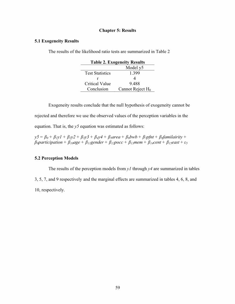
Chapter 5: Results

5.1 Exogeneity Results

The results of the likelihood ratio tests are summarized in Table 2

Table 2. Exogeneity Results Model y5

Test Statistics 1.399 r 4

Critical Value 9.488 Conclusion Cannot Reject H0

Exogeneity results conclude that the null hypothesis of exogeneity cannot be

rejected and therefore we use the observed values of the perception variables in the

equation. That is, the y5 equation was estimated as follows:

y5 = β0 + β1y1 + β2y2 + β3y3 + β4y4 + β5area + β6bwb + β7pfnt + β8familairity + β9participation + β10age + β11gender + β12pocc + β13mem + β14cent + β15east + ε5

5.2 Perception Models

The results of the perception models from y1 through y4 are summarized in tables

3, 5, 7, and 9 respectively and the marginal effects are summarized in tables 4, 6, 8, and

10, respectively.

59

Table 3. Ordered Logit Model Estimation Results for Model y1 ׀ < tParameter Estimate Standard Error t-value Pr׀

area1 -0.069 0.083 -0.83 0.406 bwb 0.710 0.457 1.56 0.120 pfnt -0.096 0.105 -0.91 0.361

familiarity -0.045 0.190 -0.23 0.815 participation -0.030 0.234 -0.13 0.900

age -0.004 0.013 -0.30 0.768 gender 0.039 0.517 0.07 0.940 pocc 0.161 0.422 0.38 0.702 mem -0.019 0.496 -0.04 0.970 cent 0.072 0.460 0.16 0.876 east 0.394 0.548 0.72 0.472

Limit1 -1.082 0.831 -1.30 0.193 Limit2 0.580 0.826 0.70 0.483

Table 4. Marginal Effects of the Variables in Model y1

Parameter

Marginal effect on the probability of

y1 = 1

Marginal effect on the probability of

y1 = 2

Marginal effect on the probability of

y1 = 3 area1 0.010 0.005 -0.015 bwb -0.145 0.097 0.048 pfnt 0.014 0.007 -0.020

familiarity 0.109 -0.136 0.027 participation 0.007 -0.004 -0.002

age 0.001 0.000 -0.000 gender -0.009 0.010 -0.001 pocc -0.036 0.023 0.012 mem 0.004 -0.003 -0.001 cent -0.015 0.010 0.005 east -0.089 0.056 0.033

As per table 3, there were no variables that were statistically significant at the 5 percent

and 10 percent levels, suggesting that the farm operators’ perception regarding whether

BMP installation and management is unfair to producers or not do not vary

systematically across farm size, producers’ familiarity or participation in conservation

programs, or other demographics.

60

Table 5. Ordered Logit Model Estimation Results for Model y2 ׀ < tParameter Estimation Standard Error t-value Pr׀

area1 0.018 0.086 0.21 0.836 bwb 0.072 0.436 0.16 0.869 pfnt -0.205 0.110 -1.87 0.062

familiarity 0.064 0.194 0.33 0.742 participation 0.076 0.229 0.33 0.741

age -0.004 0.013 -0.34 0.735 gender 0.529 0.533 0.99 0.321 pocc -0.891 0.444 -2.01 0.045 mem 0.146 0.478 0.31 0.759 cent 0.179 0.487 0.37 0.713 east -0.308 0.539 -0.57 0.567

Limit1 -0.956 0.844 -1.13 0.257 Limit2 0.914 0.844 1.08 0.279

Table 6. Marginal Effects of the Variables in Model y2

Parameter

Marginal effect on the probability of

y2 = 1

Marginal effect on the probability of

y2 = 2

Marginal effect on the probability of

y2 = 3 area1 -0.003 0.000 0.003 bwb -0.013 -0.002 0.016 pfnt 0.037 -0.001 -0.035

familiarity -0.013 0.000 0.013 participation -0.014 -0.002 0.016

age 0.000 0.000 0.000 gender -0.105 -0.004 0.109 pocc 0.155 0.044 -0.199 mem -0.026 -0.006 0.033 cent -0.032 -0.009 0.040 east 0.061 0.002 -0.063

Table 5 shows the variables statistically significant at 10 percent and 5 percent

levels were pfnt and pocc, respectively, and their marginal effects can be interpreted as

follows from table 6.

If the respondents believed that no-till is equally or more profitable than other

tillage systems, then the likelihood of the farmer agreeing that the Kansas ground water

supplies are polluted decreased by 0.035, decreased the probability of the farmer

61

remaining neutral to the statement by 0.001, and increased the probability of the farmer

disagreeing to the statement by 0.037. If the respondent’s primary occupation was

farming/ranching, then the likelihood of the farmer agreeing that the Kansas ground

water supplies are polluted decreased by 0.199, increased the probability of the farmer

remaining neutral to the statement by 0.044, and increased the probability of the farmer

disagreeing to the statement by 0.155.

Table 7. Ordered Logit Model Estimation Results for Model y3 Parameter Estimate Standard Error t-value Pr > ׀t ׀

area1 0.064 0.094 0.68 0.499 bwb 0.251 0.467 0.54 0.591 pfnt 0.083 0.118 0.71 0.481

familiarity -0.133 0.202 -0.66 0.511 participation -0.389 0.237 -1.64 0.101

age 0.008 0.014 0.61 0.544 gender 0.432 0.514 0.84 0.400 pocc 0.436 0.435 1.00 0.316 mem 0.525 0.555 0.95 0.344 cent -0.400 0.474 -0.84 0.398 east 0.222 0.571 0.39 0.697

Limit1 -1.247 0.887 -1.41 0.160 Limit2 0.468 0.879 0.53 0.594

Table 8. Marginal Effects of the Variables in Model y3

Parameter

Marginal effect on the

probability of y3 = 1

Marginal effect on the

probability of y3 = 2

Marginal effect on the

probability of y3 = 3

area1 -0.007 -0.005 0.013 bwb -0.015 -0.035 0.050 pfnt -0.007 -0.007 0.016

familiarity 0.006 0.016 -0.022 participation 0.019 0.051 -0.070

age -0.001 -0.001 0.002 gender -0.028 -0.061 0.089 pocc -0.026 -0.060 0.086 mem -0.026 -0.067 0.093 cent 0.024 0.055 -0.079 east 0.010 -0.028 0.037

62

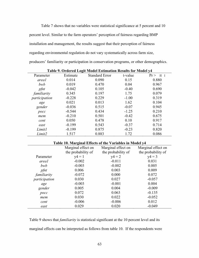
Table 7 shows that no variables were statistical significance at 5 percent and 10

percent level. Similar to the farm operators’ perception of fairness regarding BMP

installation and management, the results suggest that their perception of fairness

regarding environmental regulation do not vary systematically across farm size,

producers’ familiarity or participation in conservation programs, or other demographics.

Table 9. Ordered Logit Model Estimation Results for Model y4 ׀ < tParameter Estimate Standard Error t-value Pr׀

area1 0.014 0.090 0.15 0.880 bwb 0.019 0.470 0.04 0.967 pfnt -0.042 0.105 -0.40 0.690

familiarity 0.345 0.197 1.75 0.079 participation -0.228 0.229 -1.00 0.319

age 0.021 0.013 1.62 0.104 gender -0.036 0.515 -0.07 0.945 pocc -0.544 0.434 -1.25 0.210 mem -0.210 0.501 -0.42 0.675 cent 0.050 0.478 0.10 0.917 east -0.199 0.543 -0.37 0.714

Limit1 -0.199 0.875 -0.23 0.820 Limit2 1.517 0.883 1.72 0.086

Table 10. Marginal Effects of the Variables in Model y4

Parameter

Marginal effect on the probability of

y4 = 1

Marginal effect on the probability of

y4 = 2

Marginal effect on the probability of

y4 = 3 area1 -0.002 -0.011 0.031 bwb -0.003 -0.002 0.005 pfnt 0.006 0.003 0.009

familiarity -0.072 0.000 0.072 participation 0.030 0.027 -0.057

age -0.003 -0.001 0.004 gender 0.005 0.004 -0.009 pocc 0.072 0.063 -0.135 mem 0.030 0.022 -0.052 cent -0.006 -0.006 0.012 east 0.029 0.020 -0.049

Table 9 shows that familiarity is statistical significant at the 10 percent level and its

marginal effects can be interpreted as follows from table 10. If the respondents were

63

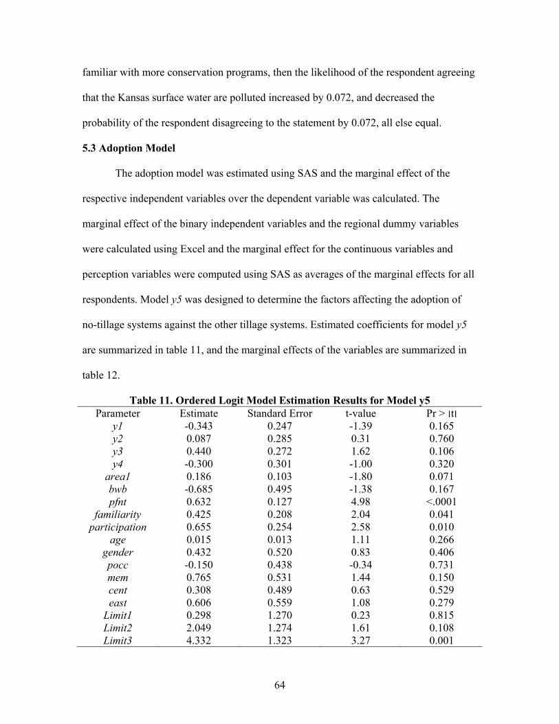
familiar with more conservation programs, then the likelihood of the respondent agreeing

that the Kansas surface water are polluted increased by 0.072, and decreased the

probability of the respondent disagreeing to the statement by 0.072, all else equal.

5.3 Adoption Model

The adoption model was estimated using SAS and the marginal effect of the

respective independent variables over the dependent variable was calculated. The

marginal effect of the binary independent variables and the regional dummy variables

were calculated using Excel and the marginal effect for the continuous variables and

perception variables were computed using SAS as averages of the marginal effects for all

respondents. Model y5 was designed to determine the factors affecting the adoption of

no-tillage systems against the other tillage systems. Estimated coefficients for model y5

are summarized in table 11, and the marginal effects of the variables are summarized in

table 12.

Table 11. Ordered Logit Model Estimation Results for Model y5 Parameter Estimate Standard Error t-value Pr > ׀t׀

y1 -0.343 0.247 -1.39 0.165 y2 0.087 0.285 0.31 0.760 y3 0.440 0.272 1.62 0.106 y4 -0.300 0.301 -1.00 0.320

area1 0.186 0.103 -1.80 0.071 bwb -0.685 0.495 -1.38 0.167 pfnt 0.632 0.127 4.98 <.0001

familiarity 0.425 0.208 2.04 0.041 participation 0.655 0.254 2.58 0.010

age 0.015 0.013 1.11 0.266 gender 0.432 0.520 0.83 0.406 pocc -0.150 0.438 -0.34 0.731 mem 0.765 0.531 1.44 0.150 cent 0.308 0.489 0.63 0.529 east 0.606 0.559 1.08 0.279

Limit1 0.298 1.270 0.23 0.815 Limit2 2.049 1.274 1.61 0.108 Limit3 4.332 1.323 3.27 0.001

64

Table 12. Marginal Effects of the Variables in Model y5 Parameter Marginal Effect

on the probability of

y5 = 0

Marginal Effect on the

probability of y5 = 1

Marginal Effect on the

probability of y5 = 2

Marginal Effect on the

probability of y5 = 3

y1 0.025 0.023 -0.005 -0.043 y2 -0.006 -0.006 0.001 0.011 y3 -0.033 -0.029 0.007 0.055 y4 0.022 0.020 -0.004 -0.037

area1 -0.014 -0.012 0.003 0.023 bwb 0.004 0.016 0.105 -0.125 pfnt -0.047 -0.042 0.009 0.079

familiarity -0.007 -0.027 -0.079 0.113 participation -0.005 -0.023 -0.118 0.146

age -0.001 -0.001 0.000 0.002 gender -0.003 -0.014 -0.076 0.093 pocc 0.000 0.004 0.025 -0.030 mem -0.004 -0.017 -0.114 0.135 cent -0.002 -0.010 -0.054 0.066 east -0.004 -0.017 -0.101 0.122

Table 11 shows the variables that were statistically significant at the 5 percent and

10 percent levels are area1, pfnt, familiarity, and participation. None of the perception

variables were statistically significant at the 10 percent level. The marginal effects of

these variables can be interpreted as follows from the table 12.

If the operated acreage of the respondents increased by 1,000 acres, then the

likelihood of the respondent adopting exclusive no-till increased by 0.023, increased the

probability of the respondent considering to adopt rotational no-till by 0.003, decreased

the probability of the respondent considering to adopt minimum tillage by 0.012, and

decreased the probability of the respondent considering to adopt more conventional

systems by 0.014, holding everything else equal.

65

If the respondents agree that the profits from no-till are equal to or more than

other systems, then the likelihood of the respondent considering to adopt exclusive no-till

increased by 0.079, increased the probability of the respondent considering to adopt

rotational no-till by 0.009, decreased the probability of the respondent considering to

adopt minimum tillage by 0.042, and decreased the probability of the respondent

considering to adopt other systems by 0.047, holding everything else equal.

If the respondent was familiar with more conservation programs, then the

likelihood of the respondent considering to adopt exclusive no-till increased by 0.113,

decreased the probability of the respondent considering to adopt rotational no-till by

0.079, decreased the probability of the respondent considering to adopt minimum tillage

by 0.027, and decreased the probability of the respondent considering to adopt other

systems by 0.007, holding everything else equal.

If the respondent participated in more conservation programs, then the likelihood

of the respondent adopting exclusive no-till increased by 0.146, decreased the probability

of the respondent considering to adopt rotational no-till by 0.118, decreased the

probability of the respondent considering to adopt minimum tillage by 0.023, and

decreased the probability of the respondent considering to adopt other systems by 0.005,

holding everything else equal.

The marginal effects for area1 suggest that larger farmers are more likely to adopt

more modern (progressive) technologies than smaller farmers. The literature suggests that

this can be explained by larger farmers facing lower credit constraint and their scale of

operation allowing them to spread the fixed cost of technology adoption. Also, the

66

marginal effects for pfnt suggest that the technology is more likely to be adopted if it is

perceived to be more profitable.

The marginal effect for participation in conservation programs is larger than those

for other factors, which can be explained by the fact that no-tillage is one of the

requirements to receive CSP payments.

5.4. Discussion

In model y2 the pfnt and pocc variables were statistically significant, and their

marginal effects seemed to suggest that the respondent perceived that no-till was more

profitable than other tillage practices, or if the respondent’s primary occupation was

farming or ranching then it decreased the probability of the respondents to agree that the

Kansas ground water supplies are polluted. The possibly contradictory results may be

reflecting that reasons why respondents may adopt no-till or other conservation tillage

systems are not related to their perceived contribution to the level of pollution of water

supply, but rather related to the perceived profitability of the conservation tillage systems,

which is what the adoption model results suggest. This association is likely stronger for

those who are primarily involved in farming or ranching. If so, this would be in contrast

to some findings that farmers are reluctant to adopt eco-friendly process for monetary

payments (e.g., Cooper and Keim, 1996).

In model y4 familiarity was the only statistically significant variable and its

marginal effect seemed to suggest that the familiarity with the conservation programs

increased the probability of the respondent to agree that Kansas surface water are

polluted. This is because conservation programs give a better understanding of the water

67

quality and this knowledge will help the farmers to assess whether or not Kansas surface

water are polluted.

In model y5 the area1, pfnt, familiarity, and participation variables were

statistically significant, and their marginal effects seemed to suggest that increase in

operating acreage, if profits are equal to or more than other tillage systems, familiarity

with and participation in conservation programs increased the probability of the

respondents to adopt no-tillage system. This may be due to various reasons such as

reduced production cost, increased yields and profits, knowledge gained from various

conservation programs, understanding the importance of adoption of BMPs, and

understanding the impact of environmental degradation and thus trying to maintain the

ecological balance.

The results of the adoption model may contribute to the interest of the USDA of

speeding up the adoption of conservation tillage practices such as no-till. From table 12

pfnt variable being statistically significant and the perception variables being not

statistically significant suggest that the adoption is motivated by farmer’s perception that

the technology is profitable and not by their perceptions of environmental policies.

Similarly, familiarity and participation being statistically significant indicated that

awareness and knowledge of the technologies through familiarity with and participation

in conservation programs motivates the farmer’s to adopt modern (innovative)

technologies.

68

Chapter 6: Conclusion

Adequate knowledge about the damages caused to the environment due to

agriculture has brought awareness among the farmers and has led to a general consensus

that farmers should be induced to adopt more environmental friendly practices. The main

objective of this study was to identify the impacts of the various factors affecting the

adoption of conservation practices in Kansas agriculture. The farmers’ decisions were

modeled as a two-stage process, consisting of the formation of perception towards

environment related practices and programs and the actual adoption of various

conservation tillage practices. Models were built using ordered logit regressions to

estimate how much the independent variables affected the farmer’s perception regarding

best management practices, surface water quality and the environmental legislation, and

then to estimate how such perceptions along with other factors affected the actual

adoption decisions.

The study was concerned with farmer’s perception for four issues: whether

mandating BMP installation and management is unfair to producers, whether or not

environmental legislation was often unfair to the producers, whether or not Kansas

ground water supplies are polluted, and whether or not Kansas surface waters were

polluted. The factors considered in this study included farm characteristics, farmer

characteristics, institutional factors, and demographic variables: farm size, presence of

bordered water bodies, profit comparison of no-till system with other tillage systems,

familiarity and participation in Conservation Reserve Program, Environmental Quality

Incentive Program, Conservation Security Program, and Kansas Buffer Initiative

69

Program, age, gender, primary occupation, membership in Kansas Farm Management

Association, and location dummies.

The results for the perception models showed that the farm operators’ perceptions

regarding whether BPM installation and management is unfair to producers or not and

whether environmental legislation is often unfair to producers do not vary systematically

across farm size, producers’ familiarity and participation in conservation programs, or

other demographics considered in the study. On the other hand, their perceptions

regarding how polluted their water supplies varied by their thoughts on relative

profitability across various tillage practices, their primary occupation, and their

familiarity with conservation programs. Specifically, the results suggested that those who

regarded no-till practices to be more profitable than other tillage practices or whose

primary occupation was farming-related tended to believe that ground water was not

polluted, and those who were less familiar with available conservation programs tended

to believe that surface water s were not polluted.

Later the study was concerned about the factors influencing the adoption of

conservation practices. Similarly, logit regression model was used to determine factors

influencing the adoption of conservation practices. As expected the adoption model y5

did capture some statistically significant factors. Specifically, the results suggested that

farmers with greater operating acreage, those who perceived that no-till was more

profitable than other tillage systems, and those with greater familiarity with and

participation in existing conservation programs were more likely to adopt more

conservation tillage systems, all else equal. Further, perceptions of fairness of

environmental regulations or the level of pollution did not impact the tillage choices.

70

The findings are subject to methodological limitations. For example, the models

might not have accounted for all relevant factors or the variables might not have captured

the actual intendedconcepts. Perhaps because of the heterogeneity in the people’s

decision, these models might have failed to capture the overall tendency, or the data set

was likely too small to capture the variability of variables among the farming population.

Further studies with larger sample size and different models can be conducted in this area

in order to check the factors influencing the farmer’s perception, adoption of

conservation practices, and the participation in various institutional programs. At the

same time, this study stresses the importance of promoting an understanding of relative

profitability of conservation tillage practices, since the adoption of no-till among the

Kansas farmers in this study were clearly motivated by perceived profitability.

71

References

Aitchison, J. and S. D. Silvey (1957), “The Generalization of Probit Analysis to the Case of Multiple Responses,” Biometrika, 44, 131-140. Ali, M.B., N.L. Brooks, and R.G. McElroy. (2000). “Characteristics of U.S. Wheat

Farming: A Snapshot” United States Department of Agriculture Economic Research Service SB968. Available at www.ers.usda.gov/publications/sb968.

Aliviar, N.G. (1972) “The use of hand tractor on lowlands rice farms in Laguna,” Journal of Agrarian Development 2, 243-254. Allmaras, R.R., R.E. Burwell, W.E. Larson, R.F. Holt, and W.F. Nelson (1966) ‘Total porosity and random roughness of the interrow zone as influenced by tillage. USDA Cons. Res. Rpt. No. 7. Amendment to the National Crop Residue Management Survey Summary (2007). Available at: http://www.conservationinformation.org/pdf/National_Summary_2007_Amendment.pdf Anonymous (2001). “Conservation Agriculture in Europe.” Available at

http://www.ecaf.org.uk Ansell, P.E., V. Bennett, D.Bull (1992) “Cryptorchidism: a prospective study of 7500 consecutive male births, 1984-8. Arch. Dis. Child., 67, 892-899. Balcet, J.C. and W. Candler (1981), “Farm Technology Adoption in Nigeria,” world Bank, Department of Western Africa Projects, Agricultural Division, Washington, D.C. Baptistia, R., and P. Swan (1998), “Do Firms in Clusters Innovate More?” Research Policy 27, 527-42. Barker, R. and R.W. Herdt. (1978) “Equity implications of technology changes [in Asia],” Agricultural economics and policies, unknown volume, p. 83-108. Batie, S.S. (1984) “Agricultural Policy and Soil Conservation: Implications for the 1985 Farm Bill,” Washington, D.C., American Enterprise Institute, Journal of Economic Issues, Vol. 22, No. 2. Besley, T. and A. Case. (1993) “Modeling Technology Adoption in Developing Countries,” American Economic Review 83:396–402.

72

Bhalla, S.S. (1979) “Farm and technical change in Indian agriculture,” In Berry, R., & Cline, W. (Eds), Agrarian structure and productivity in developing countries Baltimore: The John Hopkins University Press, pp.141-143.

Binswanger, H.P. (1978) “The economics of tractors in South Asia,” Agricultural Development Council and ICRISAT. Bouchard, C., K. Williams. And Y. Surampalli. (1992) “Nitrate Contamination of Groundwater: Sources and Potential Health Effects,” Journal AWWA, Vol. 84, Issue 9, 85-90. Bouwer, H. (1990) “Effect of water depth and groundwater table on infiltration for recharge basins,” In: Harris SC (ed) Proc 1990 Nat Conf Irrig Drain Div, Am Soc Civ Eng, Durango, Colorado, 11–13 July 1990, pp 337–384. Burger, K., P. Collier, and J.W. Gunning. (1993) “Social Learning: An Application to Kanyan Agriculture,” Centre for Study of African Economies, Institute of Economics and Statistics, University of Oxford. Burke, R.V. (1979) “Green Revolution Technologies and Farm Class in Mexico,”

Economic Development and Cultural Change, Vol. 28, No. 1, pp. 135-154

Buse, R.C. & Bromley, D.W. (1975) Applied Economics: Resource Allocation in Rural America. Ames, IA: Iowa State University Press: 623 pp. Bussey, L.E. (1978), The Economic Analysis of Industrial Projects. Englewood Cliffs, N.J.: Prentice-Hall. Cameron, L.A. “The Importance of Learning in the Adoption of High-Yielding Variety Seeds,” American Journal of Agricultural Economics 81(1999):83–94. Carter, M.R. (1994) “ A review of conservation tillage strategies for humid temperate regions,” Soil Tillage and Research 31 (4), 289-301. Clark II, E.H.; Haverkemp, J.A.; Chapman. W. (1985) Eroding soils. The off-farm impacts. Washington: The Conservation Foundation 252 p. Cochrane, Willard W. (1958) Farm Prices Myth and Reality, Minneapolis, MN: University of Minnesota Press. Cohen, W. and S. Klepper (1996) “A reprise of size and R&D,” Economic Journal 106: 925-52

73

Conley, T. and C. Udry. “Learning about a New Technology: Pineapple in Ghana,” Economic Growth Center Working Paper, Yale University, New Haven, CT, 2003. Conservation Technology Information Center, (2004). Crop Residue Management Executive Summary. Conservation Technology Information Center, West Lafayette, Indiana. Cooper, J, and R. Keim. “Incentive Payments to Encourage Farmer Adoption of Water Quality Protection Practices.” American Journal of Agricultural Economics 78 (1996): 54-64. Cotlear, D. (1986) “Technological and Institutional Change Among the Peruvian

Peasantry : A Comparison of Three Regions at Different Levels of Agricultural Development.” (Oxford: D. Phil. Thesis).

Cox, D. R. (1970), The Analysis of Binary Data. London: Methen Croppenstedt, A., M. Demeke., and M.M. Meschi. (2003) “Technology Adoption in the Presence of Constraints: the Case of Fertilizer Demand in Ethiopia,” ESA, Food and Agriculture Organization of the UN, Rome, Italy. Cutie, J. (1976) “Diffusion of Hybrid Corn Technology: The Case of El-Salvador,” International Center for Improvement of Rice and Wheat (CIMMYT), Mexico. Demir, N. (1976) “The adoption of new bread wheat technology in selected regions of Turkey.” Ervin, C.E. and D.E. Ervin. (1982) “Factors Affecting the Use of Soil Conservation Practices: Hypotheses, Evidence and Policy Implications,” Land Economics, 58: 277-292. Evenson, R. (1974), "Education and Rural Development," World Year Book of Education,

eds. P. Foster and J.R. Sheffield, Evan Brothers, London. Feder, G. “Farm Size, Risk Aversion and the Adoption of New Technology under Uncertainty,” Oxford Economic Papers 32(1980):263–83. Feder, G., R. Just, and D. Zilberman. “Adoption of Agricultural Innovations in Developing Countries: A Survey,” Economic Development and Cultural Change 33(1985):255–98.

Feder G. and R. Slade. “The Acquisition of Information and the Adoption of New Technology,” American Journal of Agricultural Economics, 1984, 66: 312-320.

74

Foster, A. and M. Rosenzweig. (1995a) “Learning by Doing and Learning from Others: Human Capital and Technical Change in Agriculture,” Journal of Political Economy 103:1176–209.

Foster, A.D., and M.R. Rosenzweig. (1995b) “Technical Change and Human-Capital Returns and Investments: Evidence from the Green Revolution.” Frankel, F.R. (1971) India’s Green Revolution: Economic Gains and Political Costs, Princeton University Press, NJ. Fuglie, K. (1999). “Conservation tillage and pesticide use in the Corn belt,” Journal of Agricultural and Applied Economics 31, 133-147.

Gafsi, S. and T. Roe. (1979) “Adoption of Unlike High-Yielding Wheat Varieties in Tunisia,” Economic Development and Cultural Change, Vol. 28, No. 1, pp. 119-133.

Gerhart, J. (1975) “The diffusion of hybrid maize in Western Kenya,” Research Report for CIMMYT. CIMMYT, Mexico City.

Gervais, J.P., R. Lambert, and F. Boutin-Dufrense. (2001) “On the Demand for Information Services: An Application to Low bush Blueberry Producers in Eastern Canada,” Canadian Journal of Agricultural Economics, 49: 217-232.

Greene, W.H. (2003) Econometric Analysis, 5th ed., Upper Saddle River, NJ: Prentice

Hall.

Griffith, D.R., J.V. Mannering, and J.E. Box. (1986) Soil and moisture management with reduced tillage. p. 19-57, Wiley, New-York.

Griliches, Z. (1957) “Hybrid Corn: An Exploration in the Economics of Technological Change,” Econometrica, Volume25, Issue 4, 501-522.

Halpin, G.T. and K.J. Bligh. (1974) “Broad-scale farm machinery usage in Western Australia,” Proceedings, Agricultural Engineering Conference ( Institution of Engineers, Australia), Sydney, 553-559.

Harman, W.L., G.J. Michels, and A.F. Wiese. (1989). “A conservation tillage system for profitable cotton production in the Central Texas High Plains,” Agron. J. 81:615– 618. Harriss, B. (1972). “Innovation adoption in Indian agriculture—The high yielding

variety program,” Modern Asian Studies, 6, pp. 54-86.. Hategekimana, B. and M. Trant. (2002) “Adoption and Diffusion of New Technology in Agriculture: Genetically Modified Corn and Soyabeans,” Canadian Agricultural Economics Society Annual Meeting, Calgary, Alberta, 30 May -1 June.

75

Hayami, T. (1981) “Causal attributions about poorly performing pupils,” Japanese Journal of Educational Psychology, 29, 287-297. Hicks, W. H., & Johnson, R. (1974). “Population growth and the adoption of new

technology in Taiwanese agriculture,” Working Papers in Economics, No. 1974-E6. Columbia, MO: University of Missouri.

Helleinger, G.K. (1975) “Smallholder Decision-Making: Tropical African Evidence,” in Agriculture in Development Theory, L.G. Reynolds (ed.), Yale University Press, New Haven, Connecticut, 27-52.

Houghton, P.D. and P.E.V. Chapman. (1986) “Glossary of terms used in soil conservation,” Soil Conservation Service of NSW, Government Printer, NSW.

Holland, J. (2004). “The environmental consequences of adopting conservation tillage in Europe: reviewing the evidence,” Agriculture, Ecosystems & Environment 103, 1-25. Hudson, N.W. (1971) Soil conservation. Cornell University Press,Ithaca, New York. Huffman, W.E. (1977) “Allocative Efficiency: The Role of Human Capital,” Quart. J.

Econ., 91: 59-79. Jamison, D.T. and P.R. Moock. (1984) "Farmer education and farm efficiency in Nepal: The role of schooling, extension services, and cognitive skills," World Development, vol. 12(1), pages 67-86, January. Jamison, D.T. and L. Lau. (1982) Farmer Education and Farm Efficiency, Baltimore: Johns Hopkins University Press. Just, R,E., and R.D. Pope. (1978) “On the Competitive Firm Under Production Uncertainty.” Australian Journal of Agricultural Economics, vol. 7(1), pages 67- 86. Khan, M.H. (1975) “The economics of Green Revolution in Pakistan,” New York (USA): Frederick. A. Kihlstrom, R.E. (1976) “Firm Demand for Information about Price and Technology,” The Journal of Political Economy, Vol. 84, No.6, 1335-1341. Kislev, Y. and N. Shchon-Bachrach. (1973) “The process of an Innovation cycle,”

American Journal of Agricultural Economics, 55 28-37.

Krause, M.A. and J.R. Black (1995) “Optimal adoption strategies for no-till technology inMichigan,” Review of Agricultural Economics, Vol. 17(3), p. 299-310.

76

Lal R (1994) “Soil erosion by wind and water: problems and prospects.” In: Lal R (ed) Soil erosion research methods, 2nd edn. Soil and Water Conservation Society, St. Lucie Press, America pp 1–9

Lal, R. (2000) “ Physical Management of Soils of the Tropics_ Priorities for the 21st century,” Soil Science. 165(3):191-207.

Lankoski, J., M. Ollikainen, and P. Uusitalo (2006) “No-till technology: benefits to farmers and the environment? Theoretical analysis and application to Finnish agriculture” European Review of Agricultural Economics 2006 33(2):193-221

Lee, L.K. and W.H. Stewart. (1985) “Landownership and the Adoption of Minimum Tillage: Reply,” American Journal of Agricultural Economics, Vol. 67, No. 3, pp. 682-683.

Lipton, M. (1976) “Agricultural finance and rural credit in poor countries,” World Development 4(7), 543-553. Lowdermilk, M. K. (1972) "Diffusion of Dwarf Wheat Technology in Pakistan's Punjab."

Ph.D. thesis, Cornell University. Maddala, G.S. (1983) “Limited Dependent and Qualitative Variables in Econometrics,”

New York: Cambridge University Press. Mannering, J.V. and M. Amemiya. (1987) “The effect of soil type and climate on tillage methods for corn.” National corn handbook, No. 53. Mannering, J. V. & Fenster, C. R. (1983). “What is conservation tillage?”. Journal of Soil Water Conservation 38:141-143. McGuirk, A.M., and Y. Mundlak. (1992) “The Transition of Punjab Agriculture: A

Choice of Technique Approach,” American Journal of Agricultural Economics, Vol. 74, No. 1, pp. 132-143.

McIsaac G., J. Michell and M. Hirschi (1995). “Dissolved phosphorus concentration in runoff from simulated rainfall on corn and soybean tillage systems,” Journal of Soil and Water Conservation, 50, 383 – 387.

Muthiah, C. (1971) “The Green Revolution Participation by Small Versus Large Farmers,” Indian Journal of Agricultural Economics 26, 25 – 34.

Neil, S. and D. Lee. (2001) “Explaining the adoption and disadoption of sustainable agriculture: The case of cover crops in northern Honduras,” Economic Development and Cultural Change, Volume 49, Issue 4; p. 793, 28 pgs

Nelson, R.R. and E.S. Phelps. (1966) “Investment in Humans, technological Diffusion

77

and Economic Growth.,” American Economics Review, 56: 69-75.

Nowak, P.J. and P.F. Korsching (1985) “The human dimensions of soil and water conservation: A historical and methodological perspective,” Advances in Soil and Water Conservation, pg. 159-184.

O’Neil, W.B. and R.S. Raucher. (1990) “Costs of groundwater contamination,” Journal of Soil and Water Conservation, Vol/Issue 45:2.

Parthasarathy, G. and D.S. Prasad. (1978) “Response to the impact of the new rice technology by farm size and tenure- Andhra Pradesh, India,” AIBA/SEARCA (Philippines), pg. 111-127.

Perrin, R. and D. Winkelmann. (1976) “Impediment to Technical Progress on Small versus Large Farms,” American Journal of Agricultural Economics, 58: 888-894.

Peterson, J.M., J.A. Fox, J.C. Leatherman, and C.M. Smith.(2007) “Choice Experiments to Assess Farmers’ Willingness to Participate in a Water Quality Trading Market” American Agricultural Economics Association Annual Meeting, Portland, Oregon, July 29-August 1, 2007. Phillips, R.E., R.L. Blevins, G.W. Thomas, W.W. Frye, and S.H. Phillips. (1980). “No- tillage agriculture,” Science (Washington, DC) 208:1108–1113. Ram, R., 1976. “Education as quasi-factor of production: the case of India’s agriculture.” PhD Dissertation.University of Chicago.

Rahm, M. and W. Huffman. (1984) “The Adoption of Reduced Tillage: The Role of Human Capital and Other Variables,” American Journal of Agricultural Economics , 66, pp. 405-413, November.

Reimund, Donn A., R.J. Martin, and C.V. Moore. (1981) “Structural change in agriculture: The experience for broilers, fed cattle and processing vegetables.” Technical bulletin 1648. Washington, DC: USDA, ERS.

Rogers, E. (1962) Diffusion of Innovations, First Edition, Simon and Schuster.

Rosenzweig, M.R. (1978), Schooling, Allocative Ability, and the Green Revolution, Eastern Economic Association, Washington, D.C.

Ruttan, V.W. (1977), “The Green Revolution: Seven Generalization,” International

Development Review Vol.19, No.4, pp.16-23.

78

Schluter, M. G. G. (1971) “Differential Rates of adoption of the New Seed Varieties in Indian: The Problem of the Small Farm,” Occasional Paper No. 47, Department of Agricultural Economics, Cornell University.

Schumpeter, J.A. (1942) Capitalism, Socialism and Democracy, New York: Harper.

Schultz, T.W. (1964) Transforming Traditional Agriculture, New Haven, CT: Yale University Press.

Schultz, T.W. (1972) “The Increasing Economic Value of Human Time,” American Journal of Agricultural Economics 54, 843-850.

Schultz, T.W. (1975) “The Value of the Ability to Deal with Disequilibria.” Journal of Economic Literature 13: 827–46.

Scobie, G. M. and Franklin, D. L. (1977) “ The impact of Supervised credit Programs on Technological change in Developing Agriculture: Reply,” Australian Journal of Agricultural Economics, 21 (1), 1 – 8.

Sharma, A. C. (1973) “Influence of Cutain Economic and Technological Factors on the Distinction of Cropped Area Under Various Crops in the Ludhiana District,” Journal of Research of the Punjab Agriculture University 10, 243 – 249.

Sidhu, S.S. (1974) “Economics of Technical Changes in Wheat Production in the Indian Punjab,” American Journal of Agricultural Economics 56, 217-26.

Smith, J., B. Anthony., G. Abraham., and M. James. (1994) “The Role of Technology in Agricultural Intensification: The Evolution of Maize Production in the Northern Guinea Savanna of Nigeria,” Economic Development and Cultural Change, Vol. 42, No. 3, pp. 537(18).

Soileau, J.M., J.T. Touchton, B.F. Hajek, and J.V. Baglio. (1994). “Sediment, nitrogen, and phosphorus runoff with conventional- and conservation tillage cotton in a small watershed,” Journal of Soil Water Conservation 48: 449-457. Spenser, D. & Byerlee, D. (1976). “Technical change, labor use and small farm

development: Evidence from Sierra Leone,” American Journal of Agriculture Economics, 58, 874-880.

Staal, S., C. Delgado, and C. Nicholson. (1997) "Smallholder dairying under transactions costs in East Africa,” World Development, vol. 25(5), pages 779-794.

Staub, W.J., and M.G. Blasé. (1974) “Induced Technological Change in Developing Agricultures: Implications for Income Distribution and Agricultural Development,” The Journal of Developing Areas, Vol. 8, No. 4, pp. 581-596.

79

Stevens, W.E., J.R. Johnson, J.J. Varco, and J. Parkman. (1992). “Tillage and winter cover management effects on fruiting and yield of cotton,” Journal of Production

Agriculture 5:570-575. Stonehouse, D.P. (1997). “Socio-economics of alternative tillage systems,” Soil & Tillage Research 43: 109-130. Stults, H.M., and R. Storhbehn (1987) “Economincs of Conservation System,” in Optimum Erosion Control at Least Cost: Proceedings of the National Symposium on Conservation Syatems, St. Joseph, Michingan: American Society of Agricultural Engineering, 227-35. Sturs, A., M. Carter and H. Johnston (1997). “A review of plant disease, pathogen interactions and microbial antagonism under conservation tillage in temperate humid agriculture,” Soil & Tillage Research 41, 169-189.

Sunding, D. and D. Zilberman.(1984) “The Agricultural Innovation Process: Research and Technology Adoption in a Changing Agricultural Sector.” (For the Handbook of Agricultural Economics). Tebrugge, F. and R.A. During. (1999) “Reducing tillage intensity — a review of results

from a long-term study in Germany,” Soil and Tillage Research, Volume 53, Issue 1, Pages 15-28.

Traore, N., R. Landry, and N. Amara. (1998). “On-farm adoption of conservation practices: The role of farm and farmer characteristics, perceptions, and health hazards,” Land Economics 74 (1): 114-127. Triplett, G.B., Jr., S.M.Dabney, and J.H. Siefker. (1996). “Tillage systems for cotton on silty upland soils,” Agron. J. 88:507–512. Triplett, G. B., S. M. Dabney, S. R. Spurlock, and L. L. Reinschmiedt. (1997) “Management systems for soil conservation and sustainable crop productivity” pp 1087-1092 IN S.S.Y. Yang, E.J. Langendoen and F.D. Shields, Jr. (eds.) Proceedings of the conference on management of landscapes disturbed by channel incision.The U of Mississippi Press. US Office of Technology Assessment, (1990). Energy Use and the US Economy, OTA- BP-E-57. US Congress, Washington, DC. (USDA-ERS) United States Department of Agriculture Economic Research Service.

(2008). Farm Household Economics and Well-Being: Beginning Farmers, Demographics, and Labor Allocations. Available at: http://www.ers.usda.gov/Briefing/WellBeing/demographics.htm.

80

(USDA-NASS) United States Department of Agriculture National Agricultural Statistics Service. (2004). 2002 Census Publications. Available at:

http://www.agcensus.usda.gov/Publications/2002/index.asp (USDA-NRCS) United States Department of Agriculture Natural Resources

Conservation Service. (2008a) “Conservation Reserve Program.” Available at: www.nrcs.usda.gov/programs/CRP.

(USDA-NRCS) United States Department of Agriculture Natural Resources

Conservation Service. (2008b) “Environmental Quality Incentives Program.” Available at: www.nrcs.usda.gov/PROGRAMS/EQIP.

(USDA-NRCS) United States Department of Agriculture Natural Resources

Conservation Service. (2008c) “Wetlands Reserve Program.” Available at: www.nrcs.usda.gov/Programs/WRP.

Van Ravenswaay, E.O. and J.R. Blend. (1997) “Using Ecolabeling To Encourage Adoption Of Innovative Environmental Technologies In Agriculture.” Van der Van, M. (1975) “Analysis of the interfarm variation in rice yields: An economic study of HYV rice production in Cavite Province, Philippines. Unpublished doctoral dissertation, Pennsylvania State University, PA. Villaume, J. (1977) “Literacy and the Adoption of Agricultural Innovations,” PhD dissertation, Harvard University, Cambridge, Massachusetts, USA. Vyas, V.S. (1975) India’s High Yielding Varieties Programme in Wheat. Mexico City:

Centro internacional del Mejoramiento de Maize y Trigo. Weil, P.M. (1970) “The introduction of ox plough in central Gambia,” In: McLaughlin, P.F. (Ed.), African Food Production Systems: Cases and Theory. Johns Hopkins University Press, Baltimore. Welch, F. (1970) “Education in Production,” Journal of Political Economy 78, 35-59. Weir, S. and J. Knight. “Adoption and Diffusion of Agricultural Innovations in Ethiopia:

The Role of Education,” April 2000, Center for the Study of African Economies WPS2000-5, Oxford. Wills, I.R. (1972) “Projection of effects of modern inputs on agricultural income and employment in a C.D. Block,” U.P, India, American Journal of Agricultural Economics 54, (3), 452-460. Wozniak, G. D. “Joint Information Acquisition and New Technology Adoption: Late versus Early Adoption,” Rev. Econ. Stat., 1993, 75: 438-445.

81

Wu, J., R. Adams, C. Kling. And K. Tanaka (2003). “Assessing the Costs and Environmental Consequences of Agricultural land Use Changes: A Site-Specific, Policy-Scale Modeling Approach,” Staff General Research Papers 10358, Iowa State University, department of economics. Wu, J., R. Adams, C. Kling and K. Tanaka (2004). “From Microlevel Decisions to Landscape Changes: An Assessment of Agricultural Conservation Policies,” American Journal of Agricultural Economics, 86, 26-41. Zhang, X., S. Fan, and X. Cai. (2002) “The Path of Technology Diffusion: Which Neighbors to Learn From?” Contemporary Economic Policy., Vol. 20, No. 4, pp. 470-478.

82

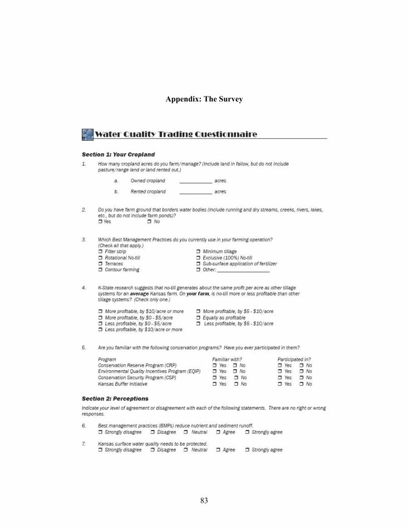
Appendix: The Survey

83

84

85

86