A094GO 769 AIR FORCE INST OF TECH WRIGHT-PATTERSON AFS OH SCHOO-ETC F/6 113INVESTIGATION OF AN IMPROVED FLUTTER SPEED PREDICTION TECHNIQUE-(TC(U)DEC 80 R K THOMSON

UNCLASSIFIED AFIT/GAE/AA/800-21 NL-mmmmmmmmmmi illiEEEEEEEEEnlllllllllllffEliEEnEEE/nlEEmhEE|hEEI.EhhEEhhmhhmhmhlmEEmmhhE~hmmhEEEE

(Li 23 JAN 1981AFITfGAE/AAf8/D-21 ,-,E AFR 190-17.

APPRO\' r4 a

9LAUREL A. LAMPELA, 2Lt, USAFDeputy Director, Public Affairs

P: In!co Intioue of Technology (ATCI',,,, % ,-:.' ;: V 3, G-H 45433 f

ror

1PfllU' fle-'ou¢ d fl

By-Distribution/Availability Codes

;Avail and/orDist Special

~, I TICELECTE

INVESTIGATION OF AN FIPROVED FEB I o 1981_FLUTTER SPEED PREDICTION

TECHNIQUE FOR DAMAGED -38 F

HORIZONTAL §TABILATORS USINC NASTRAN.

THESIS

AFIT/GAE/AA/8OD- i!Roger K;.,Thomson2Lt USAF

9 Approved for Public Release D)istribut ion tinlimit-ed

81 2 09 086

AFIT/GAE/AA/80D-21

INVESTIGATION OF AN IMPROVED

FLUTTER SPEED PREDICTION

TECHNIQUE FOR DAMAGED T-38

HORIZONTAL STABILATORS USING NASTRAN

THESIS

Presented to the Faculty of the School of Engineering

of the Air Force Institute of Technology

in Partial Fulfillment of the

Requirements for the Degree of

Master of Science

by

Roger K. Thomson, B.S.A.E

2nd Lieutenant USAF

Graduate Aeronautical Engineering

December 1980

Approved for Public Release Distribution Unlimited

Preface

Though many people were instrumental in the completion of

this work there are a Eew who should be formally mentioned for

their patience alone.

Capt. Hugh Clark Briggs, my advisor, is thanked [or in-

spiring me to undertake this project and never telling me how

far to go with it but always to take it as far as I could in

the time alloted.

In accomplishing the analysis I would first like to thank

Mr. Richard D. Talmadge of AFWAL/FIBG for his assistance in

the experimental part of this thesis. I was the first real

world user of the Modal Analysis package developed by the

. University of Cincinnati, et. al., and as I found mistakes in

the package, Mr. Talmadge corrected them.

Thanks goes to several people at AFWAL/FDL for assistance

in analytical work. I would particularily like to thank Capt.

Gene Hemmig and Mrs. Victoria Tischler for taking special in-

terest in my problems.

Lastly I would like to extend a warm thanks to my typist

Delores whose professionalism is obvious from this work.

6ii

9 Contents

INTRODUCTION................................................ 1

CHAPTER 1 VERIFICATION OF THE SERIES 3 FINITE ELEMENTMODEL UNDER STATIC LOADS....................... 3

1.1 Introduction................................... 31.2 Static Load Comparison of the Series 2

and Series 3 Stabilators....................... 41.2.1 Analytical Models.............................. 41.2.2 Loads and Boundary Conditions for the

Series 2 Influence Coefficient Model ............ 71.3 Results and Conclusions........................ 13

CHAPTER 2 MODAL ANALYSIS OF THE SERIES 3 STABILATOR .... 20

2.1 Introduction................................... 202.2 Sine Dwell Test................................ 212.2.1 Test Setup and Equipment....................... 212.2.2 Data Acquisition and Results................... 232.3 Modal Assurance Criteria....................... 232.3.1 The Modal Assurance Criteria Method ............ 232.3.2 Test Setup..................................... 2592.3.3 Data Acquisition............................... 282.3.4 Results of the MAC Test........................ 292.4 Modal Analysis Using the HP5451B Fourier

Analyser....................................... 322.4.1 Overview....................................... 322.4.2 Experimental Model and Test Setup .............. 332.4.3 Data Acquisition............................... 342.4.4 Data Reduction and Results..................... 352.4.5 Comments....................................... 382.5 Numerical Eigenvalue Analysis of the

Series 2 and Series 3 Finite Element Models 392.5.1 Analysis Method................................ 392.5.2 Results and Conclusions for the

Eigenvalue Analysis............................ 402.6 Conclusions From Mlodal Analysis ................ 42

CHAPTER 3 STEADY AERODYNAMIC ANALYSIS OF THE NASTRANSERIES 3 STABILATOR MODEI ...................... 47

3.1 Introduction .................................... 473.2 Analytical Models ............................... 473.2.1 The USSAERO Model ............................... 483.2.2 The NASTRAN Model ............................... 503.3 Method of Analysis and Results ................ 513.4 Conclusions ..................................... 54

CHAPTER 4 FLUTTER ANALYSIS OF THE T-38STABILATOR USING NASTRAN ....................... 55

4.1 Introduction .................................... 554.2 Analytical Model ................................ 554.3 Method of Analysis .............................. 574.4 Results and Conclusions ......................... 60

SUMMARY OF RESULTS AND CONCLUSIONS ......................... 61

RECOMMENDATIONS .............................................. 63

BIBLIOGRAPHY ................................................. 64

APPENDIX A: Comparison of Deflections of the Series 2and Stiffened Series 2 Models, UnderIdentical Static Loads, With ExperimentalResults ......................................... 66

APPENDIX B: Programs Used by the HP5451BFourier Analyser ................................ 73

APPENDIX C: The HP Model, Grid Pointsand Connectivity ................................ 76

APPENDIX D: Experimental and NumericallyPredicted Modes ................................. 80

APPENDIX E: Models Used for Numerical SteadyAerodynamic Analysis ........................... 115

APPENDIX F: Comparison of Experimental and NumericallyPredicted Steady Chordwise PressureDistributions .................................. 125

AIPENDTX G: Sample Output From NASTRANFlutter Analysis ............................... 139

iv

List of Figures

Figure Page

1.1 Series 3 Stab ..................................... 5

1.2 Series 2 Stab ..................................... 6

1.3 Series 3 Model, Exploded View .................. 8

1.4 Model Node Numbering Convention ................ 9

1.5 Series 2 Model, Exploded View .................. 10

1.6 Series 2 Influence Coefficient Model,Exploded View .................................... 11

1.7-11 Deflections of the Series 2 and Series 3Models Under Static Loads ..................... 14-18

2.1 Stabilator Vibration Test Setup ................ 21

2.2 Vibration Test Grid .............................. 26

2.3 Hewlett Packard HP5451B Fourier Analyser ....... 28

2.4 Sample MAC Function, 0-500 cps ................. 31

2.5 Load Cell Hammer Used in ExperimentalModal Analysis ................................... 33

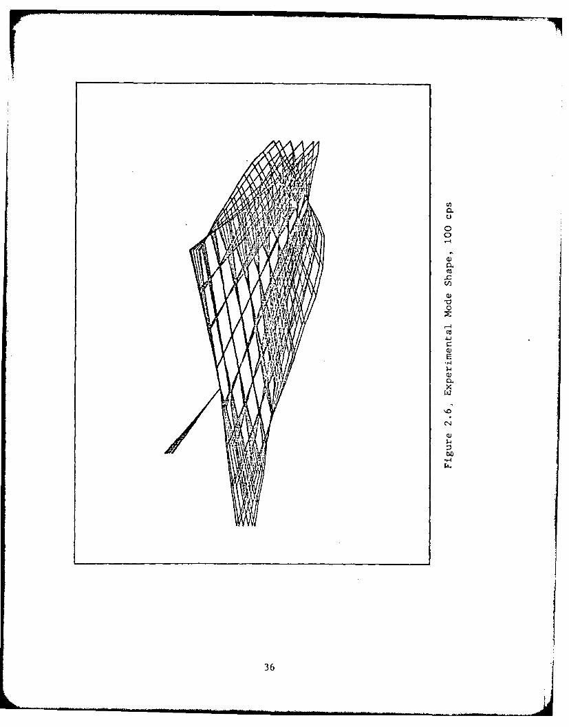
2.6 Experimental Mode Shape, 100 cps ............... 36

2.7 Experimental Mode Shape, 124 cps ............... 37

2.8 Modified Load Cell Hammer ........................ 39

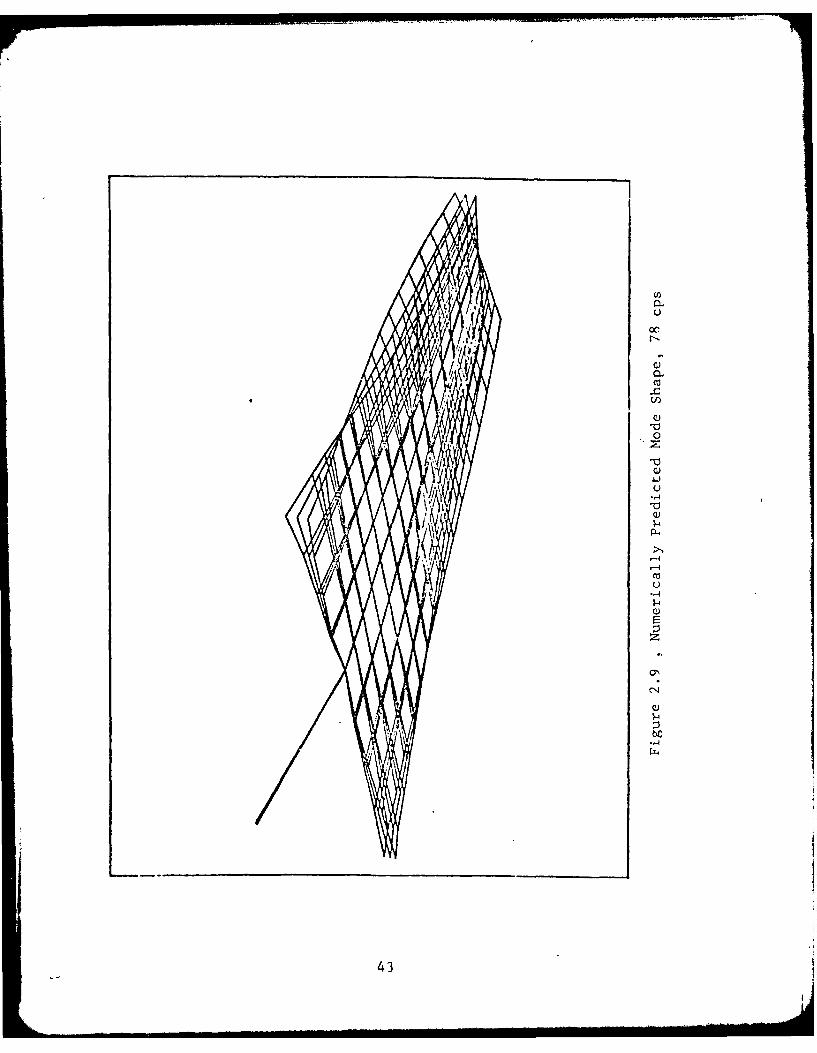
2.9 Numerically Predicted Mode Shape, 78 cps ....... 43

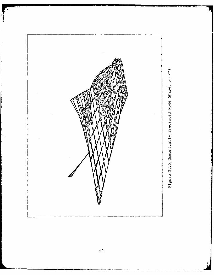
2.10 Numerically Predicted Mode Shape, 88 cps ....... 44

3.1 Experimental Wind Tunnel Model ................. 49

3.2 Comparison of Experimental and NumericallyPredicted Pressure Distributionson Stab Upper Surface ............................ 52

V

3.3 Comparison of Numerically PredictedPressure Differences on Stab ................... 53

Al-A5 Deflections of the Series 2 andStiffened Series 2 Model UnderStatic Loads .................................... 68-72

Dl-DlO Experimentally DeterminedMode Shapes, 0-400 cps ......................... 82-91

Dl1-D32 Numerically PredictedMode Shapes, 0-400 cps ......................... 93-114

Fl-F12 Experimental and NumericallyPredicted Steady ChordwisePressure Distributions ........................ 127-138

vi

9 List of Tables

Table Page

I Influence Coefficient Study, Loads and

Loading Points .................................... 12

II Experimental Apparatus ........................... 22

III Experimental Natural Frequencies forthe Series 3 Stabilator .......................... 24

IV Series 3 Experimental Grid, Fuselageand Horizontal Stabilator Stations .............. 27

V Reference and Response PointsUsed in the MAC Test ............................. 30

VI Calculated Natural Frequencies for theSeries 2 and Series 3 Stabilators ............... 41

VII Experimental and Numerically PredictedMode Shapes That Match ........................... 42

VIII Comparison of Numerically PredictedFlutter Speeds .................................... 60

vii

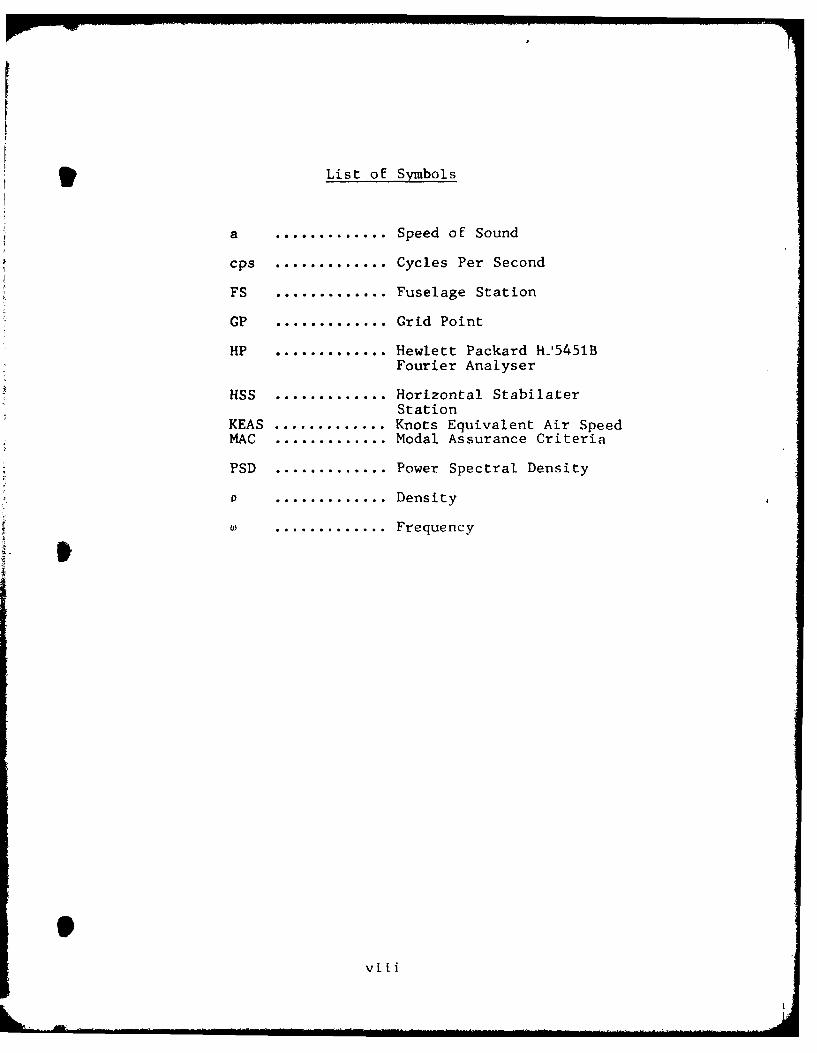
List of Symbols

a ............. Speed oE Sound

cps ............. Cycles Per Second

FS ............. Fuselage Station

GP ............. Grid Point

HP ............. Hewlett Packard H-'5451BFourier Analyser

HSS ............. Horizontal StabilaterStation

KEAS ............. Knots Equivalent Air SpeedMAC ............. Modal Assurance Criteria

PSD ............. Power Spectral Density

P ............. Density

. . Frequency

v f iAW

Abstract

This thesis concerns the development of a finite

element model of the T-38 horizontal stabilator for use

on NASTRANZ. The model is to be used to analyse degrada-

tions in flutter speed due to repair.

Static analysis has shown the rodel to be lacking in

torsional stiffness. The probable cause being the inability

of NA;TRAN plate bending elements to model torsion - -lLs.

An increase of elastic and shear moduLi of plate bending

elements In the model by 30 percent produced more accurate

results but additional investigation is necessary.

Modal analysis has pointed to a modeling error in the

root, traiLing od6e area. The affect has caused an addi-

tional node to appear on the trailing edge for modes

above 100 cps in a free-free condition. Investigation of

the steady aerodynamic pressure distribution over the

stabilator shows good correlation with experimerntal results.

A flutter analysis procedure was established and the

affects of the errors found in the stiructural model were

investigated. With no corrections made to the model, a

flutter speed equivalent to that predicted using strip theory

was achieved for the sea level condition.

ix

INVESTIGATION OF AN IMPROVED

FLUTTER SPEED PREDICTION

TECHNIQUE FOR DAMAGED T-38

HORIZONTAL STABILATORS USING NASTRAN

INTRODUCTION

Throughout the life of the T-38 the area subject to the

most scrutiny, from an aeroelastic viewpoint, has been the

horizontal stabilizer/elevator (stabilator or just stab).

Several problems exist which effect the mass distribution of

the airfoil and change its elastic characteristics. Most

prominent are the effects of water absorption, skin delamin-

ation, and cracks. Resulting changes in mass distribution,

directly or as a result of repair, effectively degrade the

flutter velocity.

To date, repair limits have been based on calculations

made using Strip Theory (Ref 1,2). In the two years prior to

July 1980, sixty-six port side and thirty-six starboard stab-

ilators were purchased as replacements at the cost of approx-

imately $10,000 each. Only three stabilators in that period

were repairable (Ref 3). It is hoped that a finite element

model can be used for more accurate, less conservative predic-

tions and that more of the stabs can be saved. Probable

savings will be proportional to the increase in accuracy

1

achieved with the new model.

This project is a follow on to the thesis by John 0.

Lassiter, AFIT/GAE/AA/80M-2 (Ref 4), who successfully con-

structed and partially verified a finite element model of the

stab for use on NASTRAN. Several problem areas were identi-

fied by Lassiter and are topics of investigation in this thesis.

Two designs of the stab were proposed in the initial de-

velopment of the T-38, referred to here as the Series 2 and

Series 3 models. Experimental information was compiled on the

Series 2 model only, while the Series 3 model was the chosen

design. For this reason, deflections of a model of the Series 2

stab under static loads is the topic of Chapter 1. Other

chapters include investigation of aspects critical to accurate

flutter speed prediction for the Series 3 stab. Chapter 2

involves a vibration analysis of the Series 3 stab both exper-

imentally and analytically. Some discussion of the vibration

characteristics of the Series 2 stab is also included to fully

integrate the relationship between the two models. Chapters

3 and 4 depart from structural aspects to consider steady flow

over the airfoil and the importanceof wing/fuselage effects in

the flutter analysis respectively.

2

CHAPTER 1

VERIFICATION OF THE SERIES 3 FINITE ELEMENT

MODEL UNDER STATIC LOADS

1.1 Introduction

Discrepancies between theoretical results From the

Series 3 finite element model and test results reported in

Ref 4 suggest Further investigation and verification of the

structural and aerodynamic models of the Series 3 T-38 stabi-

lator (Fig 1.1). Because test information has been compiled

For the Series 2 stab only, these errors can be attributed to

two sources. Either the Series 3 stab has been modeled in-

correctly and/or there is an appreciable difference between

the Series 2 (Fig 1.2) and Series 3 design.

It was assumed in Ref 4 that the Finite element model of

the Series 3 stab was in error because of a statement made in

NAI-57-59 (Ref 5) that the Series 2 and Series 3 stabs have

essentially the same stiffness. To investigate the accuracy

of this statement, a model of the Series 2 stab was constructed.

Because resonant frequency and flutter speed are both

directly related to stiffness, a great deal of attention was

focused on results that suggested the stiffness was incorrect.

Experimental results from an influence coefficient study and

static load test of the Series 2 stab (Ref 6) were the main

source of comparison. All numerical analysis for this section

was accomplished using NASTRAN Rigid Format I (Ref 7).

3

Ir

1.2 Static Load Comparison of the Series 2 and Series 3

Stabilators

1.2.1 Analytical Models

Figures 1.1 and 1.2 show the most prominent differences

between the Series 2 and Series 3 stabs. Reference 4,

Appendix A discusses the FORTRAN program BDATA that was cre-

ated and used to generate the NASTRAN bulk data deck for the

Series 3 model. For an extensive discussion of the Series 3

construction and finite element model see ReE 4:8-14. Addi-

tional modules added to BDATA include generation of 'CBAR'

and corresponding 'PBAR' cards that represent:

1. the leading edge extrusion

2. the tip rib

3. the torque tube

4. the auxiliary spar *

5. and the intermediate ribs *

Physical dimensions used to construct these modules were taken

from blueprints reproduced from aperture cards (Re[ 8).

Two models of the Series 2 stab were generated using

BDATA. One of the models was used in an eigenvalue analysis

and will be discussed later. The other is an influence co-

efficient model that contains additional grid points that

* These items are included only in the Series 2 stab

4

e.a

r4

"-4

'-to

NT*1-~

~, -~

pI

-*~:*

k-I,.

U 0

~ __ ~

~1'7, .04-i

I-

V4 ~-§~2jZ-- ~ 7' _

a -

1 i

I I

I-. t I c"JI I,

a,'-V II-I

-,. a'0

'z4

C

6

correspond to points of load applications and observed

responses. Figure 1.3 is an exploded view of the Series 3

model. Quadrilaterals represent NASTRAN 'CQUAD1' elements

while dashed lines represent 'CBAR' elements. figure 1.4

shows the node numbering convention for all the models.

Figures 1.5 and 1.6 show the two Series 2 models used. Tri-

angles in the Series 2 influence coefficient model represent

NASTRAN 'CTRIA1' elements.

1.2.2 Loads and Boundary Conditions for the Series 2

Influence Coefficient Model

Reference 4:24-28 discusses the single point constraints

which were applied to the model to simulate conditions of

svmmetry. These constraints were:

GRID POINT DISPLACEMENT ROTATION

140

145 X Z Y-AXIS

146 Y X,Z-AXIS

Constraining grid point 140 about the Y-axis removes any rota-

tion that may have been induced through the actuator assembly

or additional rotation from torque tube twist (Ref 4). Con-

straints on grid point 145 are typical of a bearing and those on

146 are used to invoke symmetry. Table I presents the static

loads and points of application.

7

3- - - 0

-- ~-1

-- ~~ UL-Ji V0

0

'~

~ V

C

0-4

'-4

8

zt.SC-linvilb 5N:

1 Z" . r1)

I-D

AUD

0

0

-4

10

Lw

Vn)

0L

TABLE I

Influence Coefficient Study, Loads and Loading Points

LOAD (ib) HSS % CHORD FIGURE

400 82.0 52.7 1.7

400 70.75 20.0 1.8

400 70.75 75.0 1.9

1200 42.25 20.0 1.10

1200 42.25 75.0 1.11

12

1.3 Results and Conclusions

Figures 1.7-1.11 show a comparison of the deflections of

the Series 2 stab and Series 3 stab under identical static

loads and boundary conditions. In these figures, solid lines

are NASTRAN results. Dashed lines are NOR-60-6 results.

Blacked in symbols and open symbols represent Series 2 and

Series 3 results respectively.

It is easily observed that the Series 2 model approximates

the experimental results more closely than the Series 3 model

but is still lacking somewhat in stiffness. Remember that the

experimental results were obtained for a Series 2 and not a

Series 3 stab.

These results suggest a lack of stiffness throughout the

model. In an attempt to make an overall correction, the elas-

tic and shear moduli of the material comprising the majority

of the stab were increased by 30 percent. The Figure 30 per-

cent will be discussed later. Parts of the structure affected

were:

1. the skin

2. outboard 30 percent of the main spar

3. the auxiliary spar

4. and the intermediate ribs

Noticeably absent From the list are the torque tube, the

majority of the main spar, and the root rib. These provide

spanwise bending stiffness. The elements listed affect an

13

CD 'oco r- '.4C

J 4N

I -X-

0 LnITI

L- 'J c a

C QNO C3 U0 ,

14.

01 '0r .

Ch 0

I Is

4~$ P .

a 0

I jl -4

lcsu

9-

co C4

150

co 40

cn 0. IfI

oC

C: Ct C4

161

0

ec

0M I~ .1 to

1 % I ,4C f L~

(so-ouj)uo~ja~U,

17U

7C

C p

II S

Ia I

I. 0

4 u1~I I

.0I 0

I S4 *00 1

'0 Cl) ~-'I *

'~0 I #0I 0w'-4II 1 1 9 .~ .,-~

U

I IU, Lfl 1CO * I U

o * k

I I)U,C,,

II S

In

1In S

U, Ig

(.4

('.4

U,U,

I I I

In* S S S S 0 5 5

S S S I S S S S(s~tpuj) uo~oI;~a

18

increase in chordwise bending stiEfness. Appendix A presents

a comparison of the Series 2 and Series 2 stiffened models

with the experimental results. Figures Ai-A5 show the stif-

fened model has approximated the experimental results much

more closely in pure bending. The largest errors result from

loads applied off the elastic axis (torsion loads). Further

'tuning' of the model is necessary to alleviate this.

It can be concluded that comparing the displacements of

the Series 3 model with experimental data for the Series 2

stab, as was done in Ref 4, is not an accurate approach. It

can also be concluded that both the Series 2 and Series 3

models are lacking in overall stiffness probably more chord-

wise than spanwise. It is probable that the error arises from

the inability of NASTRAN flat plate elements to model torsion

cells. Remember the model is composed solely of bar elements

and flat plates. In view of these findings the plate elements

may be given additional stiffness to compensate. The next

chapter contains evidence which justifies this further.

19

CHAPTER 2

MODAL ANALYSIS OF THE SERIES 3 STABILATOR

2.1 Introduction

Throughout this chapter, any mention of a stabilator will

refer directly to the Series 3 stab unless otherwise stated.

To further verify the finite element model, a comparison

of natural frequencies and mode shapes was desired. Three

experimental methods for determining frequency response infor-

mation are discussed in the following sections. Each method

is introduced followed by some discussion of the test setup,

data acquisition, and results.

In each test the stab was supported by elastic chords,

attached at each corner with adhesive, and hung parallel to

the floor (see Fig 2.1). Constraints of this type represent

a Free-Free boundary condition. Table II is a list of the

equipment used in each of the tests. Any mention of a force

gauge, accelerometer, etc. in the following sections refers

directly to those items listed.

20

Figure 2.1, Stabilator Vibration Test Setup

2.2 Sine Dwell Test

2.2.1 Test Setup and Equipment

A shaker was attached to the underside of the stab at

Fuselage Station (FS) 496.25 and Horizontal Stab Station

(HSS)35.25. A force gauge was located between the shaker and

stab and an accelerometer was placed at the outboard tip,

trailing edge. Outputs from the force gauge and accelerometer

were amplified and passed to a dual trace oscilloscope for ob-

servation of phase and variation in amplitude. Output From

the accelerometer also ran through a frequency counter.

21L|

TABLE II

Experimental Apparatus

APPARATUS MANUFACTURER MODEL COMMENTS

Fourier Spec- Hewlett- HP 5451Btrum Analyzer Packard

25 lb. shaker LingElectronics

Accelerom- Vibrametrics 1000 Aeters

Force Gauge Vibrametrics 208 A03 1 mV/lb force

Amplifiers Intech A2318 Variable gain

Oscilloscope Hewlett- HP 1707BPackard

Universal General- BandpassFilter Radio 50-1000 Hz

Terminal Tektronix TEK 4010-1

Copier Xerox Versatek Hard copiesfrom terminal

Voltmeter NLK LX-2

Power Supply AFFDL/FBG ± 15V DC

Force Gauge Piezotronics 480 APower Unit

Frequency Hewlett- HP 52451,Counter Packard

22

2.2.2 Data Acquisition and Results

Frequencies were observed to be resonant when large in-

creases in the amplitude From the response accelerometer

occurred. Each resonant Frequency encountered was also easily

audible. When a resonant Frequency was observed it was recor-

ded and an attempt was made to identify the mode oF vibration

(For lower Frequencies) by touching the surface and looking

For node lines. Table III contains the resonant Frequencies

Found From 0-300 cps.

Resonant Frequencies with node lines over the shaker

attachment point could not be identified. These were deter-

mined using the other methods presented in sections 2.3 and

2.4.

An advantage to the Sine Dwell method was that all reson-

ant modes Found were audible while some were not easily detec-

table on the oscilliscope. The audibility Factor became use-

ful when line noise at 60 cps and 180 cps (due to the use of

3-phase power in the lab) made electronic detection oF reson-

ance near these frequencies impossible.

2.3 Modal Assurance Criteria

2.3.1 The Modal Assurance Criteria Method

The Modal Assurance Criteria (MAC) and the method of sec-

tion 2.4 utilize theories in random vibration analysis. For

23

Elm

TABLE III

EXPERIMENTAL NATURAL FREQUENCIES FOR

THE SERIES 3 STABILATOR

MODAL ASSURANCE HP5451B FOURIERSINE DWELL(cps) CRITERIA(cps) ANALYSER(cps)

58 56

74

101 101 102

116 116

124 124 124

135

146

161 160 160

176 176

198 195 198

260 258 258

278

279 280

286 286

300 300

24

discussions of the theory of random vibrations the reader is

referred to Ref 9,10. The primary tool for both investiga-

tions was the Hewlett Packard HP5451B Fourier Analyser (Re[ 11).

The author was introduced to the MAC test through the

thesis by Larry B. Glenesk (Ref 12) as an accurate means of

pinpointing natural frequencies of complex structures. A dis-

cussion of the function and the parameters in the function is

presented in Ref 12:24-32. The MAC function is a measure of

the coherence between responses at two points on a structure

due to an impulse input at an arbitrary point (striking the

structure). The MAC function is defined as:

MAC - yr 2

yy(W) Srr ()

where Sry(w) represents the cross power spectral density of

the functions 'y' and 'r' in the frequency (w) domain. The

functions 'Y' and 'r' would represent the outputs of the refer-

ence and response accelerometers in this case. The bar denotes

an ensemble average of the power spectra due to excitations at

any number of different points.

2.3.2 Test Setup

Before beginning the test, the stab was marked with an

eleven spanwise by eight chordwise grid (Fig 2.2). Table IV

is a list of the grid points (GP's) and their respective HSS

and FS. This particular grid size was chosen because it was

25

--- ----- --

4

IL

26

TABLE IV

SERIES 3 EXPERIMENTAL GRID

GR ID GRIDPOINT HSS FS POINT HSS FS

1 29.0 544.5 47 56.3 531.32 29.0 536.0 48 56.3 537.03 29.0 527.5 49 56.3 542.84 29.0 519.0 50 62.0 542.45 29.0 515.3 51 62.0 537.36 29.0 510.5 52 62.0 532.17 29.0 502.0 53 62.0 526.98 29.0 493.5 54 62.0 521.79 29.0 485.0 55 62.0 516.610 33.3 487.8 56 62.0 511.411 33.3 495.8 57 62.0 506.212 33.3 503.9 58 67.8 509.913 33.3 512.0 59 67.8 514.514 33.3 520.0 60 67.8 519.115 33.3 528.1 61 67.8 523.716 33.3 536.2 62 67.8 528.317 33.3 544.2 63 67.8 532.918 39.1 543.9 64 67.8 537.519 39.1 536.4 65 67.8 542.120 39.1 528.9 66 73.5 541.721 39.1 521.4 67 73.5 537.722 39.1 513.9 68 73.5 533.723 39.1 506.4 69 73.5 529.724 39.1 498.9 70 73.5 525.625 39.1 491.4 71 73.5 521.626 44.8 495.1 72 73.5 517.627 44.8 502.0 73 73.5 513.628 44.8 509.0 74 79.3 517.329 44.8 515.9 75 79.3 520.730 44.8 522.8 76 79.3 524.231 44.8 529.7 77 79.3 527.632 44.8 536.6 78 79.3 531.033 44.8 543.5 79 79.3 534.534 50.5 543.2 80 79.3 537.935 50.5 536.8 81 79.3 541.336 50.5 530.5 82 85.0 541.037 50.5 524.2 83 85.0 538.138 50.5 517.8 84 85.0 535.339 50.5 511.5 85 85.0 532.440 50.5 505.2 86 85.0 529.541 50.5 498.8 87 85.0 526.742 56.3 502.5 88 85.0 523.843 56.3 508.3 89 85.0 521.044 56.3 514.0 90 20.0 515.345 56.3 519.8 91 10.0 515.346 56.3 525.5 92 0.0 515.3

27

fine enough to identify all node lines from 0-300 cps.

Two accelerometers were placed at various GP's. Their

outputs were amplified and monitored in the test chamber on

a dual trace oscilliscope. Outputs were also passed to a

separate room containing the HP5451B (HP, Fig 2.3) Fourier

Analyser where they were filtered to below 500 cps and

digitized.

2.3.3 Data Aquisition

One accelerometer remained stationary through the entirety

of each testing session and was referred to as the reference

accelerometer. The other was placed at arbitrary points on

the structure and was referred to as the response accelerometer.

Figure 2.3, Hewlett Packard HP54lB Fourier Analyser

28

To discover a maximum number of natural frequencies in a

test session the reference accelerometer should lie at a point

free of nodes in the desired frequency range. Following sug-

gestions from the technical staff at AFWAL/FIBG, points along

the outboard trailing edge were chosen.

Table V is a list of reference points and response points

tested. Appendix B, program 1 presents the program used by

the HP while aquiring data and processing the MAC function.

For each pair of points the responses to an impulse were

recorded and averaged in an attempt to reduce the affects of

random noise. At the end of each ensemble average the MAC

was calculated and displayed. Judgmrnt of its accuracy was

based on the number of spikes that peaked between zero and

unity. A large number of spikes appearing say between 10 and

90 percent of unity would suggest extensive noise corruption

or faulty equipment. Accurate MAC functions were produced in

hard copy, both graphically and numerically, for each pair of

points on a Versatek copier (see Fig 2.4 for a sample graph).

Some pairs required several attempts to acquire accurate

results.

2.3.4 Results of the MAC Test

Values of unity on the graph in Fig 2.4 represent natural.

frequencies. Once an approximate value [or a resonant fre-

quencv was found, the data was viewed numerically so that a

more accurate prediction could be made. When successive

29

TABLE V

REFERENCE AND RESPONSE POINTS

USED IN THE MAC TEST

REFERENCE RESPONSE

POINT POINT

66 15

66 31

66 47

66 63

66 79

66 11

66 27

66 43

66 59

66 75

82 12

82 19

82 20

82 57

30

. .... .. . . ..... .. .. . . . .. . . .. ... .. 11/ ... .. r Iii | IIIB i Il il ..... .... .. . . . . ." . . . . . .

tJo

00

~o

0

IDU~0 ',--

E 0

oX

o W 0W

*

1-4

(U E

cc

"-4

MAC

31

values of numbers within 0.2 percent of unity were encountered,

the mean frequency was recorded.

Table III contains the natural frequencies found using

the MAC test. Examination of Table III shows that the MAC

has predicted all the frequencies found in the Sine Dwell test

plus some additional ones.

2.4 Modal Analysis Using the HP5451B Modal Analysis Software

Package

2.4.1 Overview

To make a complete comparison of the Series 3 stab model

required a visual comparison of experimental and numerically

predicted mode shapes as well as a list of natural frequencies.

As shown by Glenesk (Ref 12), experimental mode shapes could

be generated using the MAC test but the procedure is arduous

and time consuming. At the suggestion of Mr. Richard D.

Talmadge, AFWAL/FIBG, it was decided to use a modal analysis

software package developed for use on the HP Fourier Analysis

System (Ref 13).

Experimental modal. analysis using such a complex system

provides enough information and topics for discussion to

easily render a thesis by itself. Because modal analysis is

not the topic of this thesis, many facts concerning the test

and results will be treated in a 'black box' fashion.

32

2.4.2 Experimental Model and Test Setup

To generate a mode shape for the stab, the HP system

required information on model geometry. Reference 10, sec-

tion 3 discusses the procedure and information required to

build a model. Appendix C presents this information for the

stab. A comparison of the coordinates listed in Appendix C

and those given in Table IV yields the respective HSS and FS.

Any mention of grid points in this section refers specifically

to this grid.

In contrast to the MAC test, the HP system requires in-

formation about the impulse to the structure as well as the

response. This required the use of a load cell hammer

(Fig 2.5) and one accelerometer. With this exception, the

test setup was identical to that of the MAC test.

Figure 2.5, Load Cell Hammer Used

in Experimental Mlodal Analysis

33

2.4.3 Data Acquisition

Throughout the test the structure was excited with the

load cell hammer at GP 7. GP 7 was chosen because of its loca-

tion along the root rib. Stiffness of the root rib, as opposed

to locations on the structure composed only of skin and honey-

comb, prevented structural deformation which would have corrupted

the impulse. In addition, GP 7 was far enough from the elastic

axis to excite both torsion and bending modes.

Five samples per ensemble per GP were used (the structure

was struck and the response measured five times) as opposed to

fifteen for the MAC test. If the test went perfectly, the

structure would have been struck 465 times. This illustrates

the reason for five averages as opposed to the fifteen used

for the MAC test.

One impulse and response ensemble was taken for each GP.

At the end of the averaging process the autocorrelation, auto-

power spectral density (PSD), cross correlation, cross PSD, and

transfer function were all calculated. At this time a decision

was made as to the accuracy of the ensemble by evaluating the

above information. Accurate transfer functions were stored by

the HP for use in data reduction after the completion of the

test. Appendix B, program 2 is the program used by the HP

during the test.

To prevent aliasing of the input information the response

was given artificial damping by multiplying it by an exponen-

tial decay function that began at unity and became zero toware

the end of the time window. The impulse was handled in a

34

similar manner by multiplying it by a truncated sine wave.

This prevented errors in the Fast Fourier Transforms.

2.4.4 Data Reduction and Results

To generate a number of mode shapes the HP system first

required a list of frequencies of interest. These could be

entered manually or picked from a representative transfer func-

tion using a display screen and cursor. The latter was used

based on the fact that not all natural frequencies found using

the earlier methods were prominent in the majority of transfer

functions.

Once a list of frequencies had been picked, a method of

curve fitting was chosen. The methods available are presented

in Ref 13, section 4. Because damping information was not

desired, the Quadrature method was used to find a relative

amplitude for each point at each of the chosen frequencies.

Results of the Quadrature fit for a particular frequency could

be previewed in tabular form along with an animated display of

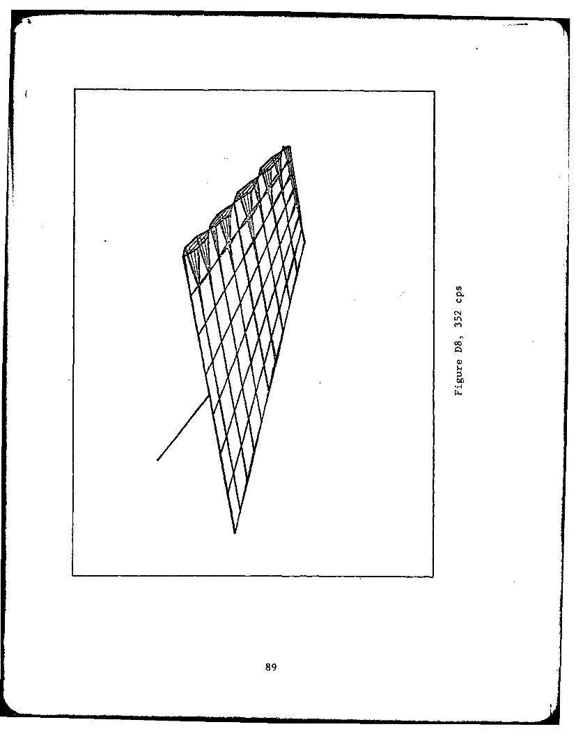
the mode shape. Figures 2.6 and 2.7 are representative of the

modes extracted using this technique. Appendix D contains

pictures of all the modes found between 0-400 cps. Some care

should be exercised in viewing the modes above 260 cps because

the grid may not have been dense enough to show all the node

lines present. The superposition of a number of displacement

amplitudes through a complete cycle highlights the node lines.

35

0

-A4

36w

'1.4

'-4

-.4

a)

L

37

2.4.5 Comments

Some question may arise as to why the procedure discussed

in this section did not yield mode shapes for all the natural

frequencies predicted. The answer lies in the inability of

the curve fitting technique to differentiate between modes

lying within ± 3 cps of each other. Another reason lies in

the fact that transfer functions in the frequency domain are

representative of the amount of energy in a mode of vibration,

i.e. low energy modes have small peaks and are hard to fit

numerically.

The first reason discussed above is the most significant

reason for not extracting a mode shape at 58 cps. Because

60 cps line noise was prominent in the lab it could not be

averaged out and consistently foiled attempts to fit the

58 cps mode. The 74 cps mode predicted by the MAC test could

not be fit because its magnitude was consistently smaller than

the 60 cps noise peak. Attempts were made to increase the

magnitude by introducing additional energy in the impulse and

low pass banding the response to below 200 cps. A new rubber

tipped hammer was designed (Fig 2.8) with an additional lumped

mass above it to accomplish this. The attempt failed because

the automatic scaling factor in the HP was set each time by

the 60 cps noise peak. This made the 74 cps mode consistently

appear diminutive.

38

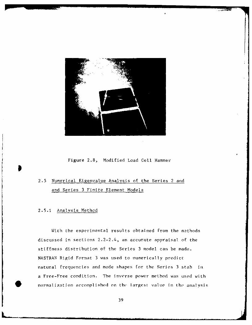
Figure 2.8, Modified Load Cell Hammer

2.5 Numerical Eigenvalue Analysis of the Series 2 and

and Series 3 Finite Element Models

2.5.1 Analysis Method

With the experimental results obtained from the methods

discussed in sections 2.2-2.4, an accurate appraisal of the

stiffness distribution of the Series 3 model can be made.

NASTRAN Rigid Format 3 was used to numerically predict

natural frequencies and mode shapes for the Series 3 stab in

a Free-Free condition. The inverse power method was used with

normalization accomplished on the largest value in the analysis

39

set (Re( 7). The NASTRAN 'SUPORT' card was used to suppress

the rigid body modes.

To further investigate the statement made in Ref 5 that

the Series 2 and Series 3 stabs have equivalent stiffness, the

natural frequencies of the Series 2 stab were also predicted.

2.5.2 Results and Conclusions for the Eigenvalue Analysis

Table VI contains the list of natural frequencies pre-

dicted numerically for the Series 2 and Series 3 stabs from

0-300 cps. A comparison shows them to be virtually identical.

These results suggest dynamic similarity while statically the

structures react differently as was shown in Chapter 1. In

this respect, the statement that the two possess equivalent

stiffness is true.

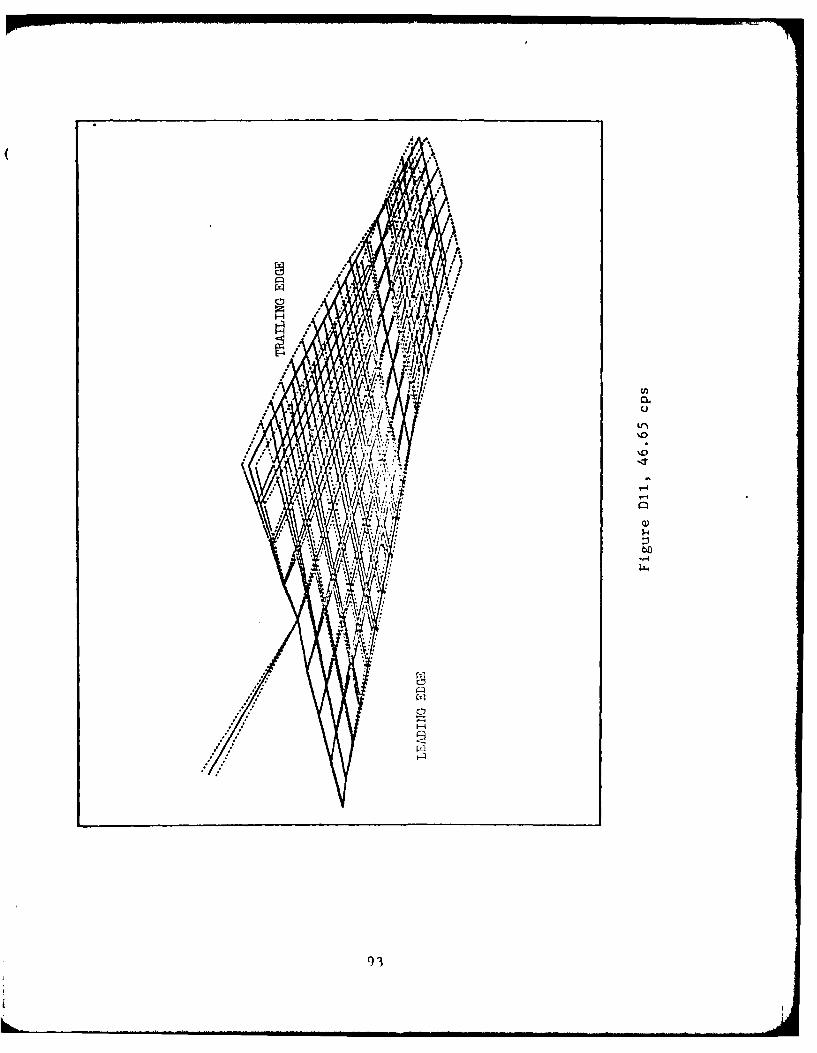
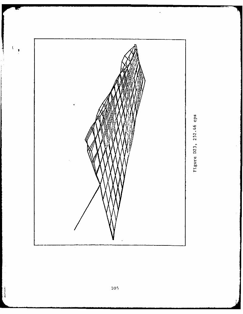
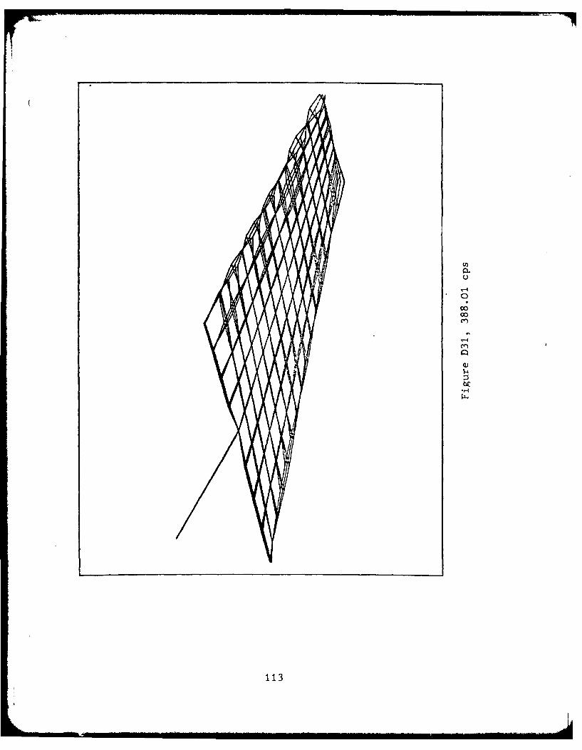
Mode shapes for the Series 3 stab were generated on a

Tektronix 4014 terminal using the interactive program

GCSNAST (Ref 11). Figures 2.9 and 2.10 are representative

mode shapes. Appendix D contains mode shapes numerically

predicted For the Series 3 stab up to 400 cps. Some care

should be exercised when viewing mode shapes above 300 cps

because the grid may not be dense enough to show all the node

lines.

4o

TABLE VI

CALCULATED NATURAL FREQUENCIES

SERIES 2 SERIES 3NATURAL FREQUENCY(cps) NATURAL FREQUENCY(cps)

46.45 46.65

78.66 77.70

88.31 88.04

115.39 112.97

122.56 121.56

126.76 124.76

147.35 144.85

168.64 167.09

189.54 188.73

199.91 200.05

213.82 214.32

224.25 224.78

252.81 252.46

258.83 259.82

280.64 279.62

310.94 309.24

41

2.6 Conclusions From Modal Analysis

Figures 2.6, 2.9 and 2.7, 2.10 are experimental and

theoretical mode shapes that appear to match exactly. Others

that show a marked resemblance are presented in Appendix D

and their relationship is shown in Table VII.

TABLE VII

EXPERIMENTAL AND NUMERICALLY PREDICTED

MODE SHAPES THAT MATCH IN APPENDIX D

EXPERI MENTAL NUMERI CAL

Fig Freq (cps) Fig Freq (cps)

D1 100 D12 77.7

D2 124 D13 88.0

D3 160 D14 113.0

D4 176 D15 121.6

D5 198 D18 167.1

D6 258 D21 214.3

D7 286 D22 224.8

D8 352 D24 259.8

While NASTRAN has predicted the shape accurately, the fre-

quencies predicted are 20-40 cps too low in the majority of

the cases. This suggests errors in the stiffness of the model

due to either the mass distribution or material stiffness

(elastic modulus).

As pointed out in Chapter 1, the Series 3 model was found

to be lacking in stiffness when subject to staitic loads. When

42

/ /"

* U.'

11

Pw

-4co

.r4

z

C)

N-

434

00

C)

E

-r4

44'

the relationship between frequency and elastic modulus for a

simple beam is considered, i.e. frequency is proportional to

the square root of Young's modulus, assuming no error in

moment of inertia, it is logical from the static results that

the predicted frequencies would be too low. This relationship

can be used to make a crude approximation to the change in

overall stiffness required to 'tune' the model into performing

correctly.

Because finite element models contain finite numbers of

nodes, it is expected that the error involved in predicting

natural frequencies gets worse as the frequency increases.

This is exhibited by the fact that the differences in frequency

of the modes predicted correctly is not a constant. For this

reason, the first experimental and numerically predicted mode

shapes that matched were used to predict a correction

(see Figs 2.6, 2.9).

ne =E lX 10 =l1.6 4 Eold

This suggests an overall increase in stiffness of 64 percent.

Believing this to be somewhat extreme it was decided to exper-

iment with a value of 30 percent.

Chapter 1, section 1.3 provides a list of the elements of

the Series 3 stab affected by an increase in shear and elastic

moduli in an attempt to correct the model. An eigenvalue

analysis of the stiffened Series 3 model was done but time

constraints and limited file space on the AFIT computer system

prevented generation of new mode shapes. However, a comparison

45

of the displacements of GP's in a normalized mode shape listed

in the NASTRAN output showed a shift of 10 cps upward For each

oF the two modes in figures 2.9 and 2.10. These were the only

modes identifiable in this manner.

Reference 4, section III provides a comparison of the

mass distribution of the model with information from N~orthrop

report NAI-58-11 (ReF 15). The correlation is good with the

exception of 50 percent additional mass in the root section.

A comparison of experimental mode shapes immediately after

124 cps and theoretical mode shapes after 88 cps shows similar

node patterns except For an extra node appearing at the inboard

trailing edge oF the theoretical model. These findings suggest

a problem in either the mass or the stiffness of the elements

in this area.

46

CHAPTER 3

VERIFICATION OF A STEADY AERODYNAMIC

MODEL OF THE T-38 STABILATOR

3.1 Introduction

Building a stabilator model for use in flutter analysis

requires consideration of the aerodynamic loads. Ultimately,

verification of an unsteady aerodynamic model is necessary.

At present the procedure for verifying an unsteady model has

not been established and no experimental results exist. To

add some confidence in the model, the steady aerodynamics will

be considered.

3.2 Analytical Models

Two models of the stab were constructed for analysis on

USSAERO (Ref 16) and NASTRAN. Appendix E contains listings

of the input required for each model. Centerline symmetry was

assumed to simulate attachment of the root to a wall, see

Milne-Thomson (Ref 17). Neglecting viscous affects, this is

an accurate representation of an airfoil in a large diameter

wind tunnel.

Both the USSAERO and NASTRAN models were designed to

47

Icorrelate with experimental results obtained at the

University of Texas at Austin (Re[ 18). Figure 3.1 (Ref 18)

illustrates the geometry of the experimental model.

3.2.1 USSAERO Model

For an extensive discussion of the aerodynamic theory

contained in USSAERO the reader is referred directly to Ref 16.

In summary, USSAERO lifting panels are modeled using a smeared

vorticity distribution varying linearly in the streamwise

direction. Singularity strengths are related to normal velo-

city by satisfying the no flow condition at the geometric cen-

ter of each panel. This provides a system of equations that

yield the strength of the singularity distribution over each

panel. The velocity and pressure coefficients are then

obtained from the singularity strengths. The aerodynamic

force on a panel is calculated by multiplying the pressure

coefficient by the panel area.

Two options are available for modeling thickness affects.

Either the upper and lower surfaces of the airfoil can be

paneled or just the mean camber line. If the mean camber line

is paneled, sources and sinks are distributed along it to sim-

ulate thickness. This method reduces the number of control.

points and the calculation time considerably and was chosen

for the analysis. No consideration for anhedral has been made

because of the small angles of attack tested.

48

- - - - - -- - - - -0

Q r--c c

ON C .00o~~~ c;C;a* 6

'-r

4-

%0 of. cvU

V06C40 4.

00 P. 00 . o c

g 136 ..

ej000. 4n a,

449

3.2.2 NASTRAN Model

Work on the initial development of the aerodynamic theory

in NASTRAN is presented in Ref 19,20. Several options are

available depending on the flight regime of interest. The

Doublet Lattice Method is used for the analysis in this chap-

ter and Chapter 4 and is summarized in the following paragraphs.

It applies only to subsonic flight.

NASTRAN unsteady lifting panels are modeled using both

a horseshoe vortex and acceleration line doublet. The horse-

shoe vortex passes through the quarter chord of each panel

with trailing vorticies entering and leaving along the panel

edges. The acceleration line doublet lies directly on the

bound part of the horseshoe vortex. A system of equations is

generated by relating the singularity strengths to the normal

velocity at the 3/4 chord, spanwise center of each panel and

staisfying the no flow condition. Once the singularity

strength is known, the Kutta-Joukowski theorem is used to find

the magnitude of the lift at the 1/4 chord of each panel. No

account is made of thickness or anhedral effects.

The NASTRAN model is made up of a structural element,

'CQUAD1', and ninety-nine aero-boxes, 'CAFRO1'. For the pro-

cedure used to generate and output the pressure coefficient

on each box, the reader is referred to the thesis by Lance E.

Chrisenger, AFIT/GAE/AA/80D-2 (Ref 21). It involves forcing

the model into a rigid pitch at the desired angle of attack

50

and approximately zero reduced frequency. Each element in the

'aeroforce' vector is divided by its respective panel area

(constant pressure panel) and output to yield values of the

pressure difference at the 1/4 chord.

3.3 Method of Analysis and Results

Experimental information from the University of Austin

allowed comparison of the chordwise pressure distribution on

the upper surface of the airfoil at two angles of attack at

Mach 0.19. Because USSAERO is a program specifically designed

for steady aerodynamic analysis, pressure distributions are

available as output for both the upper and lower surfaces of

the airfoil. NASTRAN however, computes resultant forces for

use in flutter analysis and only the pressure difference is

available.

Verification of the NASTRAN steady aerodynamic model was

accomplished by first comparing the USSAERO solution to the

experimental data for the upper surface (Fig 3.2). After

verifying the USSAERO model, a comparison of the pressure dif-

ferences predicted by USSAERO and NASTRAN was made (Fig 3.3).

Appendix F contains comparisons of theoretical and experimen-

tal results at 33.5, 66.9 and 91.7 percent semispan for two

angles of attack at Mach 0.19.

51

66.9 PERCENT SEMISPAN

0 -USSAERO

In 0-EXPERIMENTAL

C;

C

C-,

0. 00 2. 0D 00 S.D 6. 0. 00 9. 0.

PEREN COR

Fiue32 oprsn fEprmna n

Nueialwrdce Pesr itiuinOnteSa pe ufae . - .1

05

66.9 PERCENT SEMISPANC

19

C - USSAERO

C30 -NASMRN

coJ

U,

co

d

rC0. 00 2. 00 4. O0 00 7. 00 9. 0.

PECETCHR

Fiue330oprsno ueial rdce

Fisree Comprsnce o Numeicalb rdc

=2.3 M =0.19

53

3.4 Conclusions

Relatively good correlation has been achieved between

USSAERO and experimental data. Small differences lie along

the first fifteen percent and last thirty percent of the chord.

USSAERO solutions tended toward infinity at the leading edge

as is inherent in potential aerodynamic techniques. In each

case the numerical solution tends to intersect the experimen-

tal solution but not at any specific point. This suggests an

error in the moment generated over the airfoil even though an

accurate value of section lift may be predicted. One solu-

tion may be to concentrate panels toward the leading edge of

the airFoil to closer approximate a curved pressure rise in

that area.

Comparison of pressure differences across the airfoil

using NASTRAN and USSAERO show extremely close results.

USSAERO has predicted consistently higher pressure differences

than NASTRAN but the differences are small and not cause for

concern. This was expected due to the lack of thickness

affects in the NASTRAN model. These results show that

NASTRAN is modeling the aerodynamics of the airfoil correctly

fcr the steady case.

54

CHAPTER 4

FLUTTER ANALYSIS OF THE T-38

STABILATOR USING NASTRAN

4.1 Introduction

Accurate modes of vibration and natural Frequencies are

of extreme importance in determining flutter speed. Under

different flight conditions an airfoil may Flutter in any mode

but most often Flutter is encountered in one of the first

modes, i.e. torsion, bending, or a combination oF the two. In

Ref 4, "three and possibly four modes" were Found that corres-

pond closely to those of the stab in a flexible root

(1 hydraulic actuator system on) boundary condition. Resting

on these results, a method of more accurately representing the

aerodynamics of the stab in an in-flight condition was consid-

ered.

4.2 Analytical Model

The NASTRAN Flutter model is composed of the right and

left stabilators and a mock fuselage but no wing. In ReF 15

the wing is said to be stable up to 115 percent of the flight

envelope. Perturbations to the wing may cause it to oscillate

but within the flight envelope the motion damps out. At some

frequency of oscillation it is probable that flutter in the

55

stab may be excited by the wing wake. Although this may be a

problem, no attempt was made to include effects from the wing

because of the complex structural model required.

The stab is divided into six spanwise and four chordwise

panels. This rather sparse panelling scheme was chosen follow-

ing discussions with engineers at AFWAL/FDL who had achieved

good results with similar models. A change in the geometry at

the root of the stabilizer was made to straighten it. This

was required in order to panel the stab and insure that panel

side edges be parallel to the free stream. It involved a

minor shift of grid points 136-144 from their respective HSS

to HSS 27,567.

NASTRAN 'slender bodies' and 'interference bodies' are

used to model the fuselage from the wing apex to the stabila-

tor inboard trailing edge (Ref 7,20). Slender bodies are

composed of doublets placed in the flow field to simulate

fulselage thickness. A circular or elliptical fuselage cross

section can be generated by placing singularities at the cen-

terline or equidistant from the centerline in the aircraft

X-Y plane. Interference bodies are circular.

Elliptical slender bodies were chosen with major and

minor axes corresponding to the width and height of the cross

section at the stab attachment point, FS 516. Eleven slender

bodies are used to satisfy a requirement made in Ref 20,

Part II that the ratio of major axis to length be equivalent

or greater than two. This assures a number of doublets suf-

ficient to simulate at least a flat, continuous surface. The

56

fuselage cross section area is reduced linearly to zero from

the wing 1/4 chord to the wing apex to simulate, in affect,

a conical nose.

Interference bodies use the method of images to satisfy

the no flow condition through the fuselage. Reference 20

suggests the possibility of creating interference bodies of

noncircular cross section but only circular cross sections are

available in NASTRAN. The method of images involves placing

singularities within the radius of the interference body to

negate the normal wash on its surface. Three interference

bodies are used with division points at the wing apex, stab

inboard leading edge, midroot chord, and trailing edge. A

constant radius of 27.567 inches (the half width of the fuse-

lage at the stab attachment point, FS 516) was used.

4.3 Method of Analysis

Flutter analysis using NASTRAN is accomplished with

Rigid Format 10. The method of analysis is designated on the

NASTRAN 'FLUTTER' card as the 'K' method (Ref 22, section 17).

The 'K' method involves looping through values of density

ratio, reduced frequency, and Mach number. Values of flutter

velocity, damping ratio, and flutter frequency are calculated

at the end of each iteration and presented in the output.

Prior to considering the flutter problem, the aerodynamic

modal Force vector Qhh must be generated. Elements in the

57

vector are functions of reduced frequency (k) and Mach number

(M) that are specified on the 'MKEARO1' card. The vector is

segmented in blocks which represent specific M,k pairs. For-

mulation of Qhh is an expensive process and a minimum number

of Mach numbers and reduced Frequencies should be chosen.

Obviously, some prior knowledge of the flutter parameters is

desirable when making the selection.

Values of density ratio refer to a reference density

specified on the 'AERO' card. The corresponding speed of

sound is also required on this card.

At sea level:

= 1.147 x 10- 7 lbf sec

2 /in 4

a = 1.34 x 104 in/sec

The units on density should be noted. These are consistent

with the use of pounds force/square inch for elastic and shear

moduli.

Looping is controlled by the 'FLUTTER' card. The

'FLUTTER' card contains labels for 'FLFACT' cards that specify

looving parameters. Any of the values specified on the

'MKAERO' card plus additional intermediate values can be used.

If the aerodynamic modal force for a specific M, k pair is re-

quested, and it has not been generated via the 'MKAERO1' card,

two methods of interpolation are available to determine it.

These are specified on the 'FLUTTER' card as 'l or IS',

linear and surface respectively. IF more than one Mach num-

ber is used to generate the aerodynamic modal force vector

58

(it is customary to choose several values of k), surface

interpolation is used. Otherwise, linear interpolation must

be used.

The connection between the aerodynamic and structural de-

grees of freedom is accomplished using splines. For the

2-dimensional model, surface splines are used. The 'SPLINE1'

card is used to designate points in the grid to be splined.

To reduce computation time, fifteen points on the structure

were splined. No guidance is available on the actual number

of points necessary and it was thought that this number would

be sufficient. The grid points are illustrated schematically.

1 28 64 100 136

32 68 104 140 -

9 36 72 108 144

Use ofmore GP's has been found to lead to excessive computa-

tion time and core requirements making turn around time imprac-

tical. See Fig 1.4 For the precise locations.

Output is presented in tabular form with the option of

generating the classical V-g diagram. Appendix G contains a

sample in tabular form. Sign changes in the damping ratio (g)

represent points of encipient flutter. Linear interpolation

is then used to pinpoint values of flutter speed and cyclic

and reduced frequency. If no flutter condition is encount-

ered, linear extrapolation can be used to provide an educated

guess at new values of M and k to begin the process over.

59

4.4 Results and Conclusions

Results published in Ref 2 for flutter velocity of the

stab at sea level were used as initial parameters for the

flutter analysis on NASTRAN. Reference 2 uses Strip Theory

with a rigid fuselage. It is not stated in Ref 2 as to

whether wing effects were considered. Results are shown in

Table VIII.

TABLE VIII

COMPARISON OF NUMERICALLY PREDICTED

FLUTTER SPEEDS

STRIP THEORY NASTRAN

(Ref 2)

Flutter Speed (KEAS) 481.80 494

Frequency (cps) 30.51 23.8

Mach Number 0.73 0.75

The flutter speeds are very close although the frequency is

slightly off.

This indicates good correlation between the two methods

with NASTRAN predicting a higher flutter speed. These results

were achieved with no corrections in stiffness of the model.

It is expected that much less conservative values would be

calculated using a corrected model.

60

SUMMARY OF RESULTS AND CONCLUSIONS

In Chapter 1, static analysis of the Series 3 finite

element model revealed considerable lack of stiffness in chord-

* wise bending. This conclusion was arrived at through a comn-

parison of the characteristics of the Series 2 finite element

model with experimental results. The Series 2 and Series 3

models are identical with the exception of three intermediate

ribs and an auxilliary spar included in the former.

The Series 2 model was found to lack approximately 30

percent stiffness in chordwise bending. This may be attribu-

ted to modeling the structure with flat plates as opposed to

torsion cells that can support shear flow. Under identical

loads and boundary conditions, deflections of the Series 3

model are consistently greater than those of the Series 2

model. This suggests an appreciable difference in the stiff-

ness of the models and refutes the statement made in Ref 5

that they are equivalent. Because the structures are virtu-

* ally identical, and because there are no experimental static

test results for the Series 3 stab, it is assumed that the

Series 3 model is lacking in stiffness by approximately 30

percent also.

Results of Chapter 2 support the hypothesis that the

Series 3 model is lacking in stiffness. A numerical eigen-

value analysis of the model. yielded natural frequencies con-

sistently lower than those suggested from experiment.

Investigation of the higher order coupled modes revealed a

problem area at the root, trailing edge. It was shown in

Ref 4 that the mass distribution of the model compared well

with the actual stab except for a 50 percent deviation at the

root. The error is attributed to this. Experimental mode

shapes at 100 cps and 124 cps were matched with numerically

generated shapes at 78 cps and 88 cps. Other shapes show

marked resemblance all the way to 350 cps and are identified

in Table VII. The deviation in shape is also attributed to

the error discussed above.

Investigation of the pressure distribution over the stab

in a steady condition showed good results. Integration of the

chordwise pressure distribution provides accurate section lift

coefficients. However, some small deviation in section moment

exists. This can be attributed to boundary layer affects in

the experimental results.

Errors in model stiffness identified in Chapters 1 and 2

suggest predictions of flutter speed using this model would be

conservative. Results of Chapter 4 at sea level show a

flutter speed equivalent to that predicted in Ref 2 where the

method of analysis was Strip Theory. It is expected that a

corrected model would predict flutter speeds much higher than

those found using Strip Theory.

62

RECOMMENDATIONS

Experimental measurement of the displacements of the

Series 3 stab under static loads is desired. With these

results a more accurate judgment of ,-he character'istics of

the Series 3 model and corrections can be made.

No investigation of the difference between the published

section mass of the root (Ref 15) and the calculated mass of

the model at the root (Ref 4) has been attempted. Since the

two differ by an appreciable amount, and a problem has been

identified in the immediate area, some investigation is

necessary.

In addition it is desirable to -repeat the experimental

modal analysis discussed in Chapter 2, section 2.4 for bound-

ary conditions corresponding to the stab attached to the air-

craft. This would provide first hand verification of the

model in a flutter condition.

Once the structural aspects of the model. are verified,

the torsional spring stiffness of the hydraulic actuator sy-

stem, noted in Ref 14 as "critical" to the flutter speed,

should be investigated. Then an accurate assessment of the

model's capabilities in flutter speed prediction can be made.

At this point, a procedure for simulating damage and repair

can be investigated.

63

BIBLIOGRAPHY

1. Golbitz, William C. Determination of the Decrement inFlutter Speed of the Horizontal Stabilizer of the T-38AAircraft Modified with a UniForm Trailing Edge Repair.SAMME-ER-71-O11. Kelly AFB, TX: San Antonio AirLogistics Center, November 1971.

2. Burnside, O.H. T-38 Horizontal Stabilizer FlutterAnalysis Effect oTepair to Trailing Edge. SanAntonio: SoutheW t ResearEc Institute,Tanuary 1980.

3. Morgan, Don. Chief, T-38, F5 Unit System ManagementDivision (personal conversation). San Antonio, October1q80.

4. Lassiter, John 0. Initial Development for a FlutterAnalysis of Damaged T-38 Horizontal Stabilators UsingNastran. Wright-Patterson AFB, OH: Air Force Instituteof Technology, March 1980.

5. NAI-57-59. T-38A Horizontal Stabilizer. StructuralAnalysis, Hawthorne, CA: Northrop Aircraft, Inc.,March 1960.

6. NOR-60-6. Static Test of Complete Airframe [or theT-38A Airplane. Hawthorne, CA: Northrop Aircraft,Inc., March 1960.

7. NASA SP-222(04). The NASTRAN User's Manual, Level 17.Washington DC: Scientific and Technical InformationDivision, National Aeronautics and Space Administration,December 1977.

8. Aperture Cards (Code Identification Number 76823).Blueprints for the T-38 Horizontal Stabilator. KellyAFB.

9. Richardson, Mark. Modal Analysis Using Digital TestSystems. Santa Clara, CA: Hewlett Packard Co.

10. Whalev, P.E. Engineering APplications in RandomVibrations, Lecture Notes. Wright-Patterson AFB, OH:

Air Force Institute of Technology, September 1980.

11. Hewlett Packard. HP54SIB Fourier Analvser, Operatingand Service Manuals, Vol. 1-8. Santa Claral, CA:e-wlett Packard Co.

64

12. Glenesk, Larry B. The Prediction of Mass Loaded NaturalFrequencies and Forced Response of Complex, Rib-StiffenedStructures. Wright-Patterson AFB, OH: Air ForceInstitute of Technology, December 1979.

13. University of Cincinnati, et al. Modal Analysis User'sGuide. Cinncinati, OH: University of Cincinnati, April

14. McVinnie, Bill, et al. GCSNAST Manual. Wright-PattersonAFB, OH; Engineering Systems Development Department,Technical Computer and Instrumentation Center, August1979.

15. NAI-58-11. T-38A Flutter Characteristics Summary.Vibration and Flutter Analysis. Hawthorne, CA:Northrop Aircraft, Inc., June 1960.

16. Woodward, F.A. An Improved Method for the AerodynamicAnalysis of Wing-Bodv-Tail Configurations in Subsonicand Supersonic Flow. Bellevue, WA: Analytical Methods,Inc., May 1973.

17. Milne-Thomson, L.M. Theoretical Aerodynamics. New York:Dover Publications, Inc., 1973.

18. Stearman, Ronald 0. Principal Investigator, The Univer-sity of Texas at Austin (personal correspondence).Austin: August 1980.

19. AFFDL-TR-70-59, Parts I and II. Subsonic Lifting-Surface Theory Aerodynamics and Flutter Analysis ofInterfering Wing/Horizontal Tail Configurations.Hawthorne, CA; Northrop Corporation, Aircraft Division.

20. AFFDL-TR-71-5, Part II. Subsonic Unsteady Aerodynamicsfor General Configurations. Long Beach, CA: DouglasAircraft Co., Aircraft Division.

21. Chrisenger, Lance E. Calculation of Airloads for aPlexible Wing Via NASTRAN. Wright Patterson AFB, OH:Air Force Institute of Technology, December 1980.

22. NASA SP-221(04). The NASTRAN Theoretical Manual, Level17. Washington DC: Scientific and Technical Division,National Aeronautics and Space Administration, December1977.

65

APPENDIX A

COMPARISON OF DEFLECTIONS OF THE SERIES 2

AND STIFFENED SERIES 2 MODELS, UNDER

IDENTICAL STATIC LOADS,

WITH EXPERIMENTAL RESULTS

66

LEGEND

Blacked in symbols are Series 2 results.

Open symbols are NOR-60-6 experimental results.

Dotted lines are Stiffened Series 2 results.

LOAD(lb) HSS % CHORD FIGURE

400 82.0 Leading edge Al

400 70.75 20.0 A2

400 70.75 75.0 A3

1200 42.25 20.0 A4

1200 42.25 75.0 A5

" Load applied here.

67

67

o LM

Go ~Ln re nE 0

U) Enj

U2 I I

t4

-4r r-

4) CD qLA M

(Sgq:uI) O~l:OT;O

68U

InLfca -Z

C-4

0N 0

Si)~ul 1OTZOJ69 I u I ~ 0

IE I * I n I lElll Dl ii I IIIIII

C!C

W t- a')

U)I

4 4ICI

4 )0

' 0 U 4

4 C-a

700

C ; L fl

W. W

t.t4 -<co

n 0 t

C i 4

(satoui)uo~lau0

71I

0

C1In

(SI[D IO~~a;~

72I

APPENDIX B

PROGRAMS USED BY THE HP5451B

FOURIER ANALYSER

73

Cco coLf LA A

MU U) CO .4,rr

Q)

LA '.

.4 (DC

ca 0co c cr M L) 0 clir~l0) co 0

LAJClU) LA V) .4 U' U-1404.4.0 rLf I U) U.rn AC

LJW2 Ebe

<r~

74

.44

C r4flCU '-4co Cd

Lh

(Y) C0f -4

Lft

-4i

CU 0 c

-om-qm-4 ro.44 f

0

%Ai vwE W

-4-

75

APPENDIX C

THE HP MODEL

GRID POINTS AND CONNECTIVITY

76

w

C))

00

1-4 V

0±t-4 0 . cox G,

MoP

(. 0-4 0 -

2:Z Li)

nl moi (o- t-o u

t- z 0) Q -I(I) c- .1ZC'-t>

LiC cXx00 L1d LJ); 6= ..iW

0 .. .-.77

. .-. . MJMM M -n M O- M.00 - 04 _0mm mm .4m wmv V44** -,

0 T

z

- -I .UuJ u~ a W iq LA--------U wAU CM LA 014 0. aA 0 0 0 0CA0C W A A AL L J(W WU0Q000Q

O O O O O O O O O O O O Q Q G.0000.

1- f-OI # m'c m- r C .co-= --t tn n f.:AJ, ml r r- rl O-r .4083z 8 c LU(W.. c ClCJl.

87

so 5960 60 1 Z3 E ~ 187 6761 61 184 -Is9 6LIM VETO 125 62US 1 1312 6JLn ETP63 623 12G 24 ISO -16 4 64 :27 27 191 171 165 65 123 40 toe toa 2 66 66 -11.1 43 193 333 67 67 110. 56 194 34468 68 131 69 195S 49

5 9 69 122 7a 196 soa 70 70 133 '-5 197 c5771 7 1 134 Ecs 198 66872 72 135 -7 259 at973 ?3 13-S 18 gas 88

1010 74 74 137 Z3it 11 7S 73 j- Es18 1 76 76 139 t2

16 16 so 23 1-43 U11? 17 81 a) 144 7618 is $a 92 145 8712 Is 83 83 4 -G20 20 84 84 14-1 1 3E1 a1 Ss 85 49 282 2a e6 SG io 2823 23 87 67 324 24 Ba sa Is 4 525 2S 89 a9 152 54

96 3 74 r, SZ3 3 91 73 154 7022 29 9 535g 2 3 57 1SG 0630 34 94 42 157 -431 31 9S6 41Ps 132 32 19 213 33 56 26 b. 50

36 36 i 13 $337 7tea -31 14 c23 8 3 7 l p 1 6 6 1(C 633 3; 13'2 65 C. -6

439 40 I3 sa l.G 7a 40104 49 16. 84114 IC -341 41025 34 16 9 !S'2 42 106 33 1 0 243 43 107 18 1Si244 44 10 71 2

4, 9119 1 173 4 747 47 110 -S 74 s43 47 tit 90 174 52i43 49 112 91 176 fig

!'1 495 113 92 177 7951 s 114 -2I3 18 84SE S1 115 25Es -53 52 116 26 :D isS3 54 117 41 1D31 1264 64 118 42 :2 365 55119 57 113 38S3 sa %P 1 3S457 67 121 73 185 4158 52 la 74 IRS 04

79

APPENDIX D

EXPERIMENTAL AND NUMERICALLY

PREDICTED MODE SHAPES

80

EXPER IMENTAL

MODE SHAPES

81

00

'.9.

.0w

82-

c.

.- I

83

- 01

84

85

A T69 A ORCEINT OF TEC IPFLUTTERSPE TON AFBTOH C-ETC F/S 1/3INVEST16ATION OF AN IMPROVED FLUTTER SPEED PREDICTION TECHNIQUE--ETC4U)DEC 80 R K THOMSON

UNCLASSIFIED AFIT/GAE/AA/80D-21 NL

22AFI'

Emi/iImillhhlEIIIIIIIEEEEIlIIIIIIEIIEEIIIIfIE

L4

ir

Al 0T

86

00Cr)

00

87

'00

rC

88

0)

-

89

90.

I(

1/ ~' ci,

U

0

C

0'-.4

cu1.4

91

NUMERICALLY PREDICTED

MODE SHAPES

92

(

/ 4AM

*b$~'~~. I,.0 0***

,YAfl~l.

~A 1 '' *?~ / .. .

,.~. I.*~if '..

j

* ~, jg* * x*

0.

* ~i v\j U* '1 Lf'~

.5 4.

* **

* -~j.

* x 0~

* ..

'p..N!. ~' wWi

j~ 1"''V.

14

0

H

* . 14* . 14

93

A .

.7 94

00

C

95

I . 7

* 04

96

If

97

0

98

00

lit)tr:

-

99

En

00

100

C-)

1010

4 0

0

o

102

tqc

10

C','

104

,~ CL

105~

cn

c4

ticr-,4

106

cn

107~

Cj

C'4

108

c-.J

109

0

C4

.r4

110

CV)

illi

CY)

C4

0Y)

112

Ue)

cn.

113

-,4

114-

APPENDIX E

MODELS USED FOR STEADY

AERODYNAMIC ANALYSIS

115

NASTRAN STEADY

AERODYNAMIC MODEL

116

I-i r 1L4 U-4r L

L,? Li i 4i

Si I

=1 **- LL 4

Z: -L LU I _

a:~ ~ ClC

CLs t! I~ LO 'Z. ... s-AcL -jc C . ~.

1:4C. BU . 13 * 1

LL if W c

- W - I117L

IT'

- r--_ U-.!

* cv. i"

C r.._ . ,

-4 4:

,-, 7.£ ,-.-

,__. .. T. - - , ', U UJ ,

,- z. -- 17.

j',', * r- tJ'

, -'IJ._, ,_, LI (I • -A -,

_,*, _, .- i ,,U - tJ

"4 - - '-, ," •

it, Li4I

r '-i.C ,

__ *-'-Jb*,

1-- , , .- ' _ LL. . -"l ' tl -.. " r,Q L, *_. , , , - .

C-I

~- -4 4 -4 I:'h riJ 1-j

r..r- r

'IT

9-4 =99-4 9 ~.99 99 .99119 9

0. : '.[, ",- ri- '. - ' u - ' V * .' -C ,£ 0" ". rJ r . rC 0 C .".j 1,J 'J 0 " t -P,' -," -P -" ' b71 J U - ) Vi ,, .D D.. . '.- r.- .- ._

ii,.

I-r ff -* T> .(Y A-'' 7

-- .. ., 4.. _, t 4,' * 4- ..-. " - , ... L . . . "-... L ,4 .

120

I i-11j'j~i .n c r t '.fj l I Iu -t .: Q)C . rij r- .J: 1:;: '10? rCC,0-1rC , C . C -r a f 6 c. 6j j "J 1-. O CI' "' "

c. A. c,. . .

121

, .-4 -- ,--, ,-- ,-4 4 . , , , 1 ** , , -... ,--, , . --. ,-.4 ,-- ,--- 4 , .- , . ,-, .- ,.--, .--, ,.4 ,.- ,-- ,-- ,--° ,--- ,-- -. --

,'' -' -" - -r L-, -' '-, '' -, , , - £ - £ .- .. _ r- r. -r . 4, - .... .4 -¢ ,- ,. -LT ,- -

II -r.-

K. o ... >. .. . ... . . ...... . .. IT. 7., .71 I ~ *. *.T. CT- CT. 7,

.,"

J . ... II ,

. . ... . . ... . . . . . . ... . . - ... - .1

122

USSAERO STEADY

AERODYNAMIC MODEL

123

f. 'Ij

"t T., U i

..I-, . . .

-J-

CL. z. T'

*I IjT, IT, -

O-'

t.5.4 -7, 'Q C. u,Vs T .. I: *,j JT. 1.j -t

LL *, I.r. .7.'01. jjr r*t i r *

;j CL'r,

CL ir ~ C~ 124

APPENDIX F

EXPERIMENTAL AND NUMERICALLY

PREDICTED STEADY CHORDWISE

PRESSURE DISTRIBUTIONS

125

LEGEND

Figures F1-.F6 compare experimental and numerically predicted

pressure distributions on the stab upper surface.

Q - Experimental

0 - USSAERQ

Fl-F3 a =2.30 M=O.19

F4-F6 a= 4.80 M = 0.19

Figures F7-F12 compare numerically predicted pressure

differences.

0-USSAERO

0- NASTRAN

F7-F9 a2.3 0 M=Q.19

F10-F1.2 ai 4.80 M = 0.19

126

35.8 PERCENT SENISPANa)

ci

(D

. 0 00 2. 00 4. )0 00 7. 00 9. 0.

PECETCHR

CFo

'127

66.9 PERCENT SErIISPAN

co

C

c;

C4

6. 00 2 . 00 4 . 00 00 7 . 00 a . 0 .PECE-CHR

0F

12

91.7 PERCENT SEMISPAN

Ln0

.- !

F

3

112cJ

" 03

22

... . .... . . .. . .. . . . . .. .. .. . .. . . . . . .. . . . .11 [ . . . . . . .II I I .. . . . . .. .

35.8 PERCENT SEMISPAN

N

0

013

03 66.9 PERCENT SEMISPAN

C\3

C3

5F 5

13

ca 91.7 PERCENT SEMISPAN

'-4

(0

Ln

c-

PECN CHR

-F6

* 132

35.8 PERCENT SEMISPAN

-

V4

C3.

013

66.9 PERCENT SEMI SPAN

0

co

C,

Ie I

C24

a~ 8o

13

t

91.7 PERCENT SEMISPAN0

U)0

Ul)

C,

(0

C)

ca

0.0 10.0 20.0 30.0 40.0 S0.0 60.0 70.0 80.0 90.0 100.0PERCENT CHORD

F9

135

I

35.8 PERCENT SEMISPANM

o -

cll

to

'In

in

c_U:)

,2

3C

4-4

L 3-

,;)

.2

"t 8

0.0 10.0 20.0 30.0 40.0 SO.0 60.0 70.0 80.0 0.0 100.0~PERCENT CHORO

136

II

66.9 PERCENT SEMISPANcat

4ci-4

C3)

C3

413

.

91.7 PERCENT SEMISPAN

C3

C

0

0

0

C3.

0.0 10.0 20.0 30.0 40.0 GO.0 80.0 70.0 80.0 90.0 100.0P2ERCENT CHORO

F12

1 38

APPENDIX G

SAMPLE OUTPUT,

NASTRAN FLUTTER ANALYSIS

139

*544

N.b*

I;LI4Jil L U, 4-)

.45 ' ~ . C: '5 N,

N Z ~~'D 4 **5. . .

L.. M.. er C.L

-S. .4 - 4 v ev

4 j ox4--- ~C IJ* 44 2 458.

a, 64..4 cy MlM4) i

C. 0' .56 + .N D. 4CbS L.4 5 3i -o 6445.

cr''6.o crA op)414A x ...... 3

Me 65 . 0 v i j .

01 6- a)

a. Vie x 6e. g1 .

St It xc

7.Z (A x! A 5 0 y...

0 ~ ~ ~ ~ ~ 1 c57E.4.. 6*

* gem"- r .57 C . . v

-~~C 401. 5 .

-IL 60 0 C, 04 .

TV*L.4 P-. Pd I'..4.6 I.5. ~ ~ ~ . or~.n.,C Ct~s4 .V - u.s s.-5 Pr

in ' It u.*.6 I S .l aac.- ~ ~ ~ z C." 4- 0 't5A-. ~ ~ ~ I fl p - - Q N

*5i.3 ~ 66N - 51..0140

V I'IA

Roger Kent Thomson was born on 26 May 1957 in

Indianapolis, Indiana to Roger D. Thomson and Malissia A.

Thomson. Alter graduation from Richmond Senior High School,

Richmond, Indiana, in 1975 he attended Purdue University. He

graduated from Purdue on 12 May 1979 with a degrec in Acro-

iiiIcal I-:111 I neeril) .1)( Wnd ws (-)Illliss i nl 'Is aII O1'1i Cer il Lhe

U.S. Air Force the next day through the ROTC program. 2nd 'Lt.

Thomson was assigned to the Air Force Institute of Technology,

School of Engineering, on 5 June 1979 in the Graduate Aeor-

nautical Engineering Program.

Permanent address:

C/O Malissia A. Thomson234 South 8th StreetRichmond, Indiana

47374

141

€, C uF(Iv V C 1 A' .1P A I(IN 0V T I', I-A .i (IIh, . ,,,

REPORT DOCUMEtTATION PAC;I= A., ..W.

I i t.JIII IItlMII II (,OVI ACL I NO M I ,I II A 'A f

4. 1"llaI/ I i-.d itt , l ,,) YI y I I 1 0 ( 1111AII If L I 1,I I JVl. I, f )

]1j,',,J[(GAT10, OF AN 11M1'k'OVGD ]'LU'i.T SITIIED 1 T I1 .v,]DICi.ON ']I' IN.QUE' FOl DA AG':]) 'r-38fi(]ZON'A.'PL, STAI3ILATOIS USING NAST 1UN 6 U.II i, .o 4, IN 0 I ,f N T Num iI"

A A", 'I . U CONI10 lA C1(1 C,11 UPAi.' .UMPAH R

hI1jer K. Thomson

T i FIO.MIN(i OFNCANI ZATION N AMI AND ADDfL SS IU I (.lA-1 f L EM-NT I ld'JI . T TASKARI.A 8 W(t UNIT NUMIJ: h

Air Force Institute of Technology(kAFIT-EN) AL OKUi UU

Wright-Patterson AFB, 011 45433

11. CONTROLLING OFFICE NAME AND ADDRESS 12. RLPORT DATE

Deceni'ber , 1 9P01 4 N IIA1I I 1 If tA t -

1 4114 M.('U1 r ONIt , AULNi Y NAM . A A [if !-'.;(11 t/ .,It l If ..... I.. li. l)!,i.) II. U~l Y LL At~ (.1 Ih.I. taj t)

UnclassifiedI. UI:CL ASIFICATION DOWNORAD.INO

SC.it 1DU L L

16. DISTRIBUTION STATEMENT (of thil. Irpwott)

Approved for public release; distribution unlimited

Il. DISTRIOUTION STATCMENT (ol flt, abstract ferlaod iI loIIIk 20. of difhlre,t Iron, HI.gport)

18. SUPPLEMENTARY NOTES

Approved for public release; lAW 190-17FREDRIC C. LYNCH, Major, USAFDirector of Public Affairs 3 0 DEC 1980

19. KEY WORDS (Co.iinue on reverse side #I neceaisary and Identity by block nauribor)

USSAERONASTRANStabilatorMode ShapeFlutter Analysis

20, ABGTRACT (Coamtinue on revere, side It necessary and identify by block nwosber)

This thesis concerns the development ol a finite clementmodel of the T-38 horizontal stabilator [or use on NASTRAN.The model is to be used to analyse degradations in flutterspeed due to repair.

Static analysis has shown the model to be lacking intorsional. stiffness. The probable cause being the inabilityof NASTRAN plate bending elements to model torsion cells.

DD ,JAM, 1473 ITIO. OF I NOV6ISOUSOLETE

bLCu4.TY CLA I IC I )ON Of1 I 41b. I'A(.L (11h... Vist., ,.,.,J)

SCCURITY CLASSIFICATION OF THIS PAG,(Ha. D&e. Ef,.or.d)

An increase of elastic and shear moduli of plate bendingelements in the model by 30 percent produced more accurateresults but additional investigation is necessary.

Modal analysis has pointed to a modeling error in theroot, trailing edge area. The affect has caused an additionalnode to appear on the trailing edge for modes above 100 cps ina free-free condition. Investigation of the steady aerodynamicpressure distribution over the stabilator shows good correlationwith experimental. results.

A flutter analysis procedure was established and theaffects of the errors found in the structural model wereinvestigated. With no corrections made to the model, a flutterspeed equivalent to that predicted using strip theory wasachieved for the sea level condition.

SECUHITY CLA&SiFICAIOW OF T-,- PAf. (l'hon J10 tnletod)