AN IMPROVED METHOD OF INVESTIGATION OF COMBUSTION PARAMETERS

IN A NATURAL GAS FUELLED SI ENGINE WITH EGR AND H2 AS ADDITIVES

by

WEI-CHIN CHANG

A thesis submitted to The University of Birmingham

for the degree of

DOCTOR OF PHILOSOPHY

School of Manufacturing and Mechanical Engineering The University of Birmingham

Birmingham B15 2TT England

August 2002

University of Birmingham Research Archive

e-theses repository This unpublished thesis/dissertation is copyright of the author and/or third parties. The intellectual property rights of the author or third parties in respect of this work are as defined by The Copyright Designs and Patents Act 1988 or as modified by any successor legislation. Any use made of information contained in this thesis/dissertation must be in accordance with that legislation and must be properly acknowledged. Further distribution or reproduction in any format is prohibited without the permission of the copyright holder.

ABSTRACT

An improved approach to the classical Rassweiler and Withrow’s mass fraction burned model

and an improved data acquisition/processing procedure are employed with the intention of

increasing precision while retaining simplicity. A new method to predict the trends of MFB

and emissions, based on the online analysis of cylinder pressure is introduced. A diagnostic

method to study the heat release rate in a natural gas fuelled engine has been developed for

future use.

Natural gas fuelled vehicles are environmentally friendly and it is possible to use a high

compression ratio engine with all its associated benefits for efficiency. However, one of the

problems associated with the use of natural gas is NOx emission. EGR can be used to reduce

NOx, but it leads to unstable combustion. The stability problem can be resolved by the

addition of hydrogen, which can be provided by fuel reforming. Based on the beneficial

effects of exhaust gas fuel reforming, the effects of EGR, H2 and H2/CO as additives to

natural gas are analysed and discussed in terms of combustion indicators derived by the new

diagnostic method, in particular in terms of combustion duration (CA for 5/50/95% MFB),

IMEP and cycle by cycle variation (COV of IMEP, COV of peak pressure).

ACKNOWLEDGMENTS

I would like to thank Dr. Miroslaw Wyszynski for his academic supervision and guidance throughout my study, and Dr. A. Megaritis for his encouragement and help. I wish to thank my colleague, Mr. Steven Allenby (soon to be Ph.D), for his friendly support and help with the English language. I also wish to thank Mr. Eric Chiang, the chairman of Chun-Hsin Electric and Machinery Mfg. Corp., Taiwan, for the financial support in the first year of this study. Finally, I have to thank my long-suffering wife, Pin-Wei, for her unfailing support, and my son, Chun-Hsiang, and my daughter, Yu-Hua, for forgiving me for being unable to be a good farther during the last few years. Without their support and everlasting love, this work would not have been possible.

i

CONTENTS

1. INTRODUCTION..................................................................................................1

1.1. The Work Presented in this Thesis..............................................................................4

2. LITERATURE SURVEY .......................................................................................6

2.1. Acquisition of Volume and Pressure Data ..................................................................6 2.1.1. Engine Volume............................................................................................................7

2.1.1.1. Clearance Volume...............................................................................................7 2.1.1.2. Optical Crankshaft Encoder................................................................................7

2.1.2. Piezoelectric transducer..............................................................................................8 2.1.3. Ionisation Sensor ......................................................................................................10 2.1.4. Estimation of Pressure Data .....................................................................................12

2.2. Some Aspects of Acquiring Accurate Pressure vs. Volume Data............................16 2.2.1. Choosing the Number of Cycles to Analyse.............................................................17 2.2.2. Phasing of TDC ........................................................................................................19 2.2.3. A Reference Datum for Piezoelectric Transducer Signals .......................................21 2.2.4. Crank Angle Resolution ...........................................................................................23 2.2.5. Finding the End of Combustion through Pressure Traces ........................................24 2.2.6. Raw Data Smoothing................................................................................................26

2.3. Generating Information from Acquired Data..........................................................32 2.3.1. Indicated Mean Effective Pressure (Gross and Net IMEP)......................................32

2.3.1.1. Coefficient of Variation of IMEP (COVIMEP) ...................................................33 2.3.2. Mass Fraction Burned Calculation ...........................................................................34 2.3.3. Heat Release Rate.....................................................................................................38 2.3.4. Emissions Prediction ................................................................................................41 2.3.5. Studies of Combustion Behaviour............................................................................42

2.4. Natural Gas as an Alternative Fuel for SI Engine...................................................45

2.5. Effects of EGR and Hydrogen as Additives on Engine Combustion .....................49 2.5.1. Exhaust Gas Recirculation (EGR)............................................................................49 2.5.2. Hydrogen (H2) ..........................................................................................................50 2.5.3. Trade-off Effects of EGR and H2 .............................................................................51

ii

3. IMPROVED METHODS OF CALCULATION OF THE MASS FRACTION BURNED RESULT............................................................................................53

3.1. Deduction from the Classic Mass Fraction Burned Method ..................................53 3.1.1. R&W’s Model ..........................................................................................................53 3.1.2. The Novel r-R&W Model Proposed in this Thesis ..................................................57

3.2. Method of Linear Changes of Polytropic Indices ....................................................59

3.3. Finding the End of Combustion ................................................................................60

3.4. Determination of the Polytropic Index .....................................................................64 3.4.1. Compression and Expansion Polytropic Index.........................................................66

3.5. Ignition Delay and Burn Duration............................................................................68 3.5.1. Ignition Delay...........................................................................................................68 3.5.2. Burn Duration...........................................................................................................69 3.5.3. MFB Definitions Used in the Program.....................................................................70

4. DESCRIPTION OF EXPERIMENTAL METHOD AND PROCEDURE ...............71

4.1. Hardware Arrangement.............................................................................................71 4.1.1. Engine.......................................................................................................................71 4.1.2. Fuel Supply...............................................................................................................73 4.1.3. Temperature Monitoring...........................................................................................74 4.1.4. Emissions Measurement ...........................................................................................75 4.1.5. Data Acquisition Rig ................................................................................................76

4.1.5.1. Data Acquisition Board ....................................................................................76 4.1.5.2. Pressure and Crank Angle Acquiring Instruments............................................77

4.2. Program Description ..................................................................................................81 4.2.1. Data Acquisition .......................................................................................................81 4.2.2. IMEP Calculation .....................................................................................................82 4.2.3. Mass Fraction Burned...............................................................................................83

4.3. Test Procedure.............................................................................................................86

5. EFFECTS OF IMPROVED APPROACHES ON COMBUSTION DURATION CALCULATION.................................................................................................89

iii

5.1. Effects of Basic Operating Conditions......................................................................89 5.1.1. Engine Speed ............................................................................................................90 5.1.2. Gross IMEP ..............................................................................................................91 5.1.3. Ignition Timing.........................................................................................................91

5.2. Effects of Data Processing and Analysis Methods ...................................................98 5.2.1. Data Smoothing Methods .........................................................................................99 5.2.2. Polytropic Index Method..........................................................................................99 5.2.3. Pressure Phasing.....................................................................................................103 5.2.4. Pressure Pegging ....................................................................................................105

5.3. Validation of EOC point – the Comparison with 95% Mass Fraction Burned ..127

6. EFFECTS ON COMBUSTION INDICATORS WHEN ADDING H2/EGR INTO NATURAL GAS FUELLED ENGINE ..............................................................128

6.1. Combustion Characteristics of Natural Gas..........................................................128

6.2. The Combustion Indicators Affected when Adding EGR.....................................131 6.2.1. IMEP, MFB and Cycle by Cycle Variations ...........................................................131 6.2.2. Emissions - NO, UHC and CO...............................................................................132

6.3. Adding H2 as an Additive in NG Fuel .....................................................................138

6.4. Combined effects of EGR & H2 – Fuel Reforming Simulation ............................140 6.4.1. Adding EGR and H2 Alternately – Investigation of the Trade-off Effect...............140

6.4.1.1. Test 1.1 - Fixed Ignition Timing Test .............................................................141 6.4.1.2. Test 1.2 - Maximum Thermal Efficiency Test ................................................142

6.4.2. Test 2 - Reformed Fuel Test....................................................................................143 6.4.3. Peak Pressure..........................................................................................................144 6.4.4. Emissions Control ..................................................................................................145

7. APPLICATIONS OF DIFFERENTIAL PRESSURE DATA ...............................151

7.1. Prediction of MFB ....................................................................................................152 7.1.1. By Derivative Value................................................................................................152 7.1.2. By Integral of 2nd Derivative Values.......................................................................153

7.2. Emissions pattern prediction...................................................................................158

iv

7.2.1. Nitric Oxide ............................................................................................................159 7.2.2. Carbon Monoxide...................................................................................................159

8. CONCLUSIONS AND FUTURE WORK ..........................................................162

8.1. Conclusions ...............................................................................................................162 8.1.1. Accuracy of Improved Methods.............................................................................162 8.1.2. The Correlations between Additives and Combustion Related Indicators .............163 8.1.3. Using Differential Pressure Data to Predict the MFB and Emissions....................163

8.2. Future Work..............................................................................................................164 8.2.1. Data Acquisition Rig ..............................................................................................164 8.2.2. Program ..................................................................................................................165 8.2.3. MFB Model ............................................................................................................166 8.2.4. Emissions prediction ..............................................................................................166

REFERENCES........................................................................................................168

APPENDIX - A ........................................................................................................177

APPENDIX - B ........................................................................................................179

v

NOMENCLATURE / SUBSCRIPT Nomenclature: 9PWS 9 points weighted smoothing method BDC, ABDC, BBDC Bottom dead centre, After BDC, Before BDC TDC, ATDC, BTDC Top dead centre, After TDC, Before TDC BMEP Brake mean effective pressure (bar) CA Crank angle (degree) CNG Compressed natural gas CO Carbon monoxide COV, COVIMEP Coefficient of variation, COV of IMEP DAQ Data acquisition DC Direct current EGR Exhaust gas recirculation EOC End of combustion EVO Exhaust valve open HC Hydrocarbon Hz Hertz (frequency unit) IG Ignition IMEP Indicated mean effect pressure (bar) IVC Inlet valve close LPF Low pass filter method NG Natural Gas NOx, NO Oxide of nitrogen, Nitric oxide MBT Minimum advance for best torque (crank angle) MFB Mass fraction burned (-) P Cylinder pressure (bar) PMEP Pumping mean effective pressure (bar) R&W Rassweiler and Withrow model SI Spark ignition SOC Start of combustion T Temperature (K) TDC Top dead centre UHC Unburned hydrocarbon V Engine cylinder volume (m3)

vi

WOT Wide open throttle cps Cycles per second deg. Degree n Polytropic index nc Compression polytropic index ne Expansion polytropic index p Average value of relevant parameter P Pmax Peak pressure (bar) psi pounds per square inch r-R&W Revised R&W model rc Compression ratio s Standard deviation x MFB θpmax CA of peak pressure

θxb5 CA of 5% MFB λ air/fuel ratio γ Ratio of specific heats

Subscript:

c Referring to clearance volume n Referring to net IMEP g Referring to gross IMEP s Referring to swept volume

vii

LIST OF FIGURES

Figure 2-1 Details of piezoelectric pressure transducer [25]. ............................................15

Figure 2-2 Effect of crank angle resolution and number of cycles on mean IMEP error in low load low speed [41]. ..................................................................................30

Figure 2-3 IMEP error as a function of a TDC error [57]. .................................................30

Figure 2-4 T-S diagram with different TDC phase lags [46]. ............................................31

Figure 2-5 log P – log V diagram with properly phased TDC at motoring condition........31

Figure 2-6 The pressure inside cylinder during combustion can be divided to two sources: combustion (xc) and piston movement (xp).......................................................43

Figure 2-7 Cyclic variations of normalized IMEP with θxb5 and Xbcor. [64]. ....................44

Figure 3-1 The comparison of Polytropic indices between petrol and natural gas fuel at 2000 rpm, 2 bar IMEP, produced from K4 engine for this thesis.....................58

Figure 3-2 The upper part of mass fraction burned profile, the traces fro the left to the right gradually approach to the final EOC position with one crank angle degree increment. .........................................................................................................62

Figure 3-3 Flow diagram of the EOC approaching process...............................................63

Figure 3-4 Effects of different polytropic index methods on deciding the pressure increment of K4 engine ....................................................................................67

Figure 3-5 log P – log V diagram in normal firing condition; the polytropic indices nc and ne in compression and expansion strokes respectively are derived by the best fit curve fitting. .................................................................................................67

Figure 4-1 Intake piping arrangement of K4 engine. .........................................................79

Figure 4-2 Schematic diagram of data acquisition rig. ......................................................80

Figure 4-3 Dead weight calibration results of pressure transducer and charge amplifier set with the similar setting of charge amplifier in the tests....................................80

Figure 4-4 Block diagram of three main functions in the program....................................84

Figure 4-5 A partial front panel of the in-house program. .................................................85

viii

Figure 5-1 The variation of MFB between two speeds at two different comparison bases, i.e. time and crank angle. Operating conditions: 2 bar IMEP, IG timing: -31° ATDC, COVIMEP ≤ 5 %. ...................................................................................94

Figure 5-2 Comparison between two different IMEP at 2000 rpm, IG timing: -31° ATDC. (A) P-V diagram (B) MFB. ..............................................................................94

Figure 5-3 Correlations between ignition timing, IMEP and COVIMEP (A) Standard and Lower speed conditions, (B) Higher load condition.........................................95

Figure 5-4 Correlation between ignition timing and average peak pressure in three different operating conditions; the related NO content in exhaust is showing the same tendency.............................................................................................95

Figure 5-5 Comparison of 5%, 50% and 95% MFB in three different conditions.............96

Figure 5-6 MFB profile vs. ignition timing in standard condition.....................................96

Figure 5-7 MFB profile vs. ignition timing in lower speed condition. ..............................97

Figure 5-8 The variation of Polytropic index against ignition timing in two different operating conditions. k1 - compression polytropic index, k2 – expansion polytropic index................................................................................................97

Figure 5-9 The difference between raw data and smoothed data methods in 2nd derivative of pressure data in the standard operating condition. (A) Raw data vs. LPF, (B) 9PWS vs. LPF.................................................................................................107

Figure 5-10 The effects of data smoothing on MFB calculation results with different polytropic index methods. Engine operated in the standard condition. .........108

Figure 5-11 The effects of data smoothing on MFB calculation results with different polytropic index methods. Engine operated in higher load condition............109

Figure 5-12 The effects of data smoothing on MFB results with different polytropic index methods. Engine operated in lower speed condition (IG timing: -31° CA ATDC). ......................................................................................................... 110

Figure 5-13 The comparison of MFB results between different polytropic index methods and revised R&W model. Data smoothing method: raw data; engine operated in standard condition. Percentages stand for the deviation from the r-R&W model. ......................................................................................................... 112

ix

Figure 5-14 The comparison of MFB results between different polytropic index methods and revised R&W model. Data smoothing method: low pass filter; engine operated in standard condition. Percentages stand for the deviation from the r-R&W model. ................................................................................................ 113

Figure 5-15 The comparison of MFB results between different polytropic index methods and revised R&W model. Data smoothing method: 9 points weighted smoothing; engine operated in standard condition. Percentages stand for the deviation from the r-R&W model................................................................... 114

Figure 5-16 The comparison of MFB results between different polytropic index methods and revised R&W model. Data smoothing method: LPF + 9PWS; engine operated in standard condition. Percentages stand for the deviation from the r-R&W model. ................................................................................................ 115

Figure 5-17 The comparison of MFB results between different polytropic index methods and revised R&W model. Data smoothing method: raw data; engine operated in higher load condition. Percentages stand for the deviation from the r-R&W model. ......................................................................................................... 116

Figure 5-18 The comparison of MFB results between different polytropic index methods and revised R&W model. Data smoothing method: low pass filter; engine operated in higher load condition. Percentages stand for the deviation from the r-R&W model. ................................................................................................ 117

Figure 5-19 The comparison of MFB results between different polytropic index methods and revised R&W model. Data smoothing method: 9 points weighted smoothing; engine operated in higher load condition. Percentages stand for the deviation from the r-R&W model................................................................... 118

Figure 5-20 The comparison of MFB results between different polytropic index methods and revised R&W model. Data smoothing method: LPF + 9PWS; engine operated in higher load condition. Percentages stand for the deviation from the r-R&W model. ................................................................................................ 119

Figure 5-21 The comparison of MFB results between different polytropic index methods and revised R&W model. Data smoothing method: raw data; engine operated in lower speed condition (IG timing: -31° CA ATDC). Percentages stand for the deviation from the r-R&W model.............................................................120

x

Figure 5-22 The comparison of MFB results between different polytropic index methods and revised R&W model. Data smoothing method: low pass filter; engine operated in lower speed condition (IG timing: -31° CA ATDC). Percentages stand for the deviation from the r-R&W model..............................................121

Figure 5-23 The comparison of MFB results between different polytropic index methods and revised R&W model. Data smoothing method: 9 points weighted smoothing; engine operated in lower speed condition (IG timing: -31° CA ATDC). Percentages stand for the deviation from the r-R&W model............122

Figure 5-24 The comparison of MFB results between different polytropic index methods and revised R&W model. Data smoothing method: LPF + 9PWS; engine operated in lower speed condition (IG timing: -31° CA ATDC). Percentages stand for the deviation from the r-R&W model..............................................123

Figure 5-25 (A) Variations of MFB profile (B) Trend of each MFB stage (C) Table of required CA on each MFB stage – caused by phasing error in standard engine operating condition. ........................................................................................124

Figure 5-26 The influence of phasing error on the polytropic index. ................................125

Figure 5-27 (A) Deviations of IMEP and COVIMEP (B) Variations of P-V diagram – caused by phasing error in standard operating condition. ..........................................125

Figure 5-28 Correlation between IMEP error and phasing error........................................126

Figure 5-29 The effect of reference absolute pressure error on (A) MFB calculation, (B) Polytropic index values. .................................................................................126

Figure 6-1 Similar combustion behaviours between methane and natural gas fuel, engine ran at 2000 rpm, 4.3 bar IMEP and ignition timing -31° CA ATDC, (A) P-V diagram (B) MFB profile................................................................................130

Figure 6-2 The variations of required crank angles to reach MFB stage in three base line tests. ................................................................................................................130

Figure 6-3 (A) EGR versus COVIMEP, the trend lines of mass fraction burned show an increasing tendency when 50% MFB is retained at 10° CA ATDC. (B) MFP profiles versus crank angle from igniting. Engine ran at 2000 rpm, 2 bar IMEP, ignition timing varied as necessary.................................................................135

xi

Figure 6-4 Comparisons of the cycle by cycle variations among three engine operating conditions (A) MBT timing, (B) MBT timing with EGR and (C) advanced spark timing to keep 50% MFB at 10° CA ATDC, in all cases the engine ran at 2000 rpm, 2bar IMEP. ....................................................................................136

Figure 6-5 The variations of NO and HC in emissions when applied advanced ignition timing method to EGR application. Engine operating condition: 2000 rpm, 2 bar IMEP, spark ignition varying to keep 50% MFB at 10° CA ATDC. ........137

Figure 6-6 Variations of CO, NO and HC emissions with air/fuel ratio, engine ran without EGR at 2000 rpm, 2 bar IMEP, ignition timing: 31° CA BTDC. ...................137

Figure 6-7 The variation of required crank angles in each MFB stage with increasing hydrogen, engine ran at 2000 rpm, 2 bar IMEP, ignition timing varying to keep 50% MFB at 10° CA ATDC. ..........................................................................139

Figure 6-8 Variations of NO and HC emissions with hydrogen in the inlet charge, engine ran at 2000 rpm, 2 bar IMEP, ignition timing varying to keep maximum thermal efficiency. ..........................................................................................139

Figure 6-9 The variations of pressure versus volume when adding hydrogen or EGR into the NG fuel, engine ran in the standard condition..........................................140

Figure 6-10 (A) Required crank angle degrees versus EGR. Comparison of different MFB stages. Real line shows the test procedures in which EGR and H2 were added alternately. (B) P-V diagram and (C) MFB profile are comparisons between base line and test final condition. Engine ran in the standard condition with COVIMEP fluctuating about 5% (Test 1.1).......................................................146

Figure 6-11 Required crank angle degrees versus EGR. Comparison of different MFB stages. Real line shows the test procedures in which EGR and H2 were added alternately. Engine ran in the standard condition with COVIMEP fluctuating about 5%, ignition timing was adjusted to keep 50% MFB at 10° CA ATDC (Test 1.2). ........................................................................................................147

Figure 6-12 Required crank angle degrees versus EGR. Comparison of different MFB stages. Real line with H2/CO volume percentages shows the test procedure in which EGR and H2/CO were added alternately. Engine ran in the standard condition with COVIMEP fluctuating about 5%. (Test 2). ...............................148

xii

Figure 6-13 Required crank angle degrees versus peak pressure. Comparison of 5%, 95% and total mass fraction burned........................................................................149

Figure 6-14 EGR versus emissions. Comparison of three combined effects tests.............150

Figure 7-1 Pressure data patterns of natural gas fuelled engine. (A) Original pressure data (B) 1st derivative of pressure data (C) 2nd derivative of pressure data (D) Relevant window of 2nd derivative of pressure data. Data shown are from a baseline test of the standard operating condition............................................156

Figure 7-2 2% MFB position on the second differential pressure curve. Comparison of (A) lower speed and (B) higher load conditions. ..................................................156

Figure 7-3 Correlation between MFB and integral of 2nd derivative of pressure data.....157

Figure 7-4 The deviation between the integral value of 2nd derivative of pressure data and the subtraction value of 1st derivative of pressure data. .................................157

Figure 7-5 Correlations of NO and the integral of 2nd derivative of pressure data divided by peak pressure .............................................................................................160

Figure 7-6 CO versus the integral of 2nd derivative of pressure data. ..............................161

xiii

LIST OF TABLES

Table 2-1 Specification of ideal transducer by [25]..........................................................15

Table 2-2 The definitions of percentages of mass fraction burned...................................44

Table 2-3 Typical composition of natural gas [80]. ..........................................................48

Table 2-4 (A) Thermodynamic and (B) combustion properties of hydrogen, methane and gasoline [81]. ....................................................................................................48

Table 3-1 Definitions of Parameters in R&W’s assumptions [14]. ..................................58

Table 4-1 Specifications of the K4 Medusa engine. .........................................................71

Table 4-2 Specification of optical shaft encoder...............................................................72

Table 4-3 Main compositions of natural gas used in the tests. .........................................73

Table 4-4 List of temperature monitoring points. .............................................................74

Table 4-5 Instruments list of emissions analysis. .............................................................75

Table 4-6 Relevant specifications of data acquisition board: NI PCI-MIO-16E-4...........77

Table 4-7 Settings for charge amplifier.............................................................................78

Table 5-1 The differences of MFB calculation between raw and smoothed data under diferent operating conditions and polytropic index values............................. 111

Table 6-1 Emissions results of base line and final stable condition in Test 1.1..............142

Table 6-2 Emissions results of base line and final stable condition in Test 1.2..............143

Table 6-3 Emissions results of base line and final stable condition in Test 2.................144

Table 6-4 Percentage reductions of three emissions. Results shown are the comparisons between the baseline and the stable condition with similar EGR content in each test...................................................................................................................145

Table 7-1 Estimated EOC point by 1st and 2nd derivative value methods.......................153

Table 7-2 The linear equations of trend lines. Each equation represents the correlations between the integral of 2nd derivative of pressure data and required crank angles at relative MFB stage. .........................................................................154

1

1. INTRODUCTION

Although the internal combustion engine has been developed for more than one century,

combustion conditions inside the engine cylinder are still not precisely predictable yet, mainly

because of the cycle-by-cycle variations from unexpected fuel-air mixture charge and the

unknown heat transfer condition. Moreover, research has emphasized alternative fuels

recently. The combustion behaviour might be very different from traditional fuels, i.e. petrol

and diesel. An optical engine is capable of being used to explore the combustion process

inside the cylinder by observing the flame behaviour with a high-speed camera [1] or

in-cylinder flow in a motored engine with particle image velocimetry [2]. However, the costs

of such an engine and instruments are prohibitively high for most engine research, and the

destruction of engine is impracticable for a performance diagnosis on a mass produced engine.

A good experimental rig that can accurately collect combustion information from a firing

engine and also foretell the emissions trends will be a helpful diagnostic tool for alternative

fuel (i.e. natural gas) engine development.

Amann [3] said that the cylinder pressure indicator is the most important diagnostic tool in

engine investigation, he also presented several applications using pressure data as engine

performance indicators. The extent of pressure data applications covers a very wide range, e.g.

closed loop feedback control using pressure signals as a data source [4], heat release related

2

analysis [5-7], abnormal combustion detection [8, 9] and emission prediction [10], all have

been well studied and proved accurate.

Obviously using pressure data alone will not yield too much meaningful information from the

cylinder, it has to be associated with some other parameters collected simultaneously from the

engine. The time resolved pressure data is known to be useful, from which much information

can be extracted regarding combustion phenomena inside the engine cylinder, and none of the

expensive instruments, installations and troublesome hardware modifications are necessary.

Combustion is the most important chemical behaviour inside an engine cylinder, a series of

quick reactions are triggered by a spark plug in an SI engine. Engine combustion is complex

and happens suddenly in a very short time, the behaviour of the flame strongly depends on the

inlet charge mixtures. Understanding the combustion progress can help researchers to develop

better knowledge for car engine design and improved emission results. By using an IBM

compatible personal computer and modern data acquisition rig, real-time data acquisition and

analysis become feasible. With some attention to signal collecting and processing, e.g.

phasing of TDC, data smoothing, etc, the dependable data can be collected, therefore a simple

and reliable analysis method is an essential process to not only present an engine combustion

performance, but also to predict the emissions behaviour.

Apparently, many researchers have made efforts to simulate the combustion conditions for

3

engine research. Heywood [11, Ch. 14] classified these models into thermodynamic and fluid

dynamic groups, Ramos [12, Ch. 4] defined thermodynamics and dimensional models for

spark-ignition engine research work, Chow and Wyszynski [13] used the first and second

thermodynamics law to distinguish their differences. There are so many different mathematic

methods to model the engine combustion, but only a few can be applied to real time analysis

because of calculation time or information availability problems. One of the real-time

applicable models is by Rassweiler and Withrow [14]. They produced a widely used classic

method to analyse burn rate and reveal combustion conditions inside engine. Regardless of

heat transfer and crevice leakages but still maintaining accuracy, the pressure rise due to

combustion is proportional to the mass of burned charge.

Since first discovered in the U.S.A. at Fredonia, New York, in 1821, natural gas has, in just

half century after World War II, become a highly demanded energy source. Natural gas is

currently the basis for 19% of the world's energy supply, and it has long been used as a

stationary engine fuel. Because natural gas is a much cleaner fuel than gasoline/diesel, it

could perhaps bridge a transition to a renewable-powered transportation system.

The application of natural gas as a vehicle fuel is not popular enough so far, there are a few

automakers producing natural gas fuelled automobiles, however the fuel supply infrastructure

is still not widespread for this kind of vehicle, nevertheless it is optimistic to investigate the

4

use of natural gas because of the abundant stock and low emission characteristics. Even for

the newest fuel cell car development, producing hydrogen by catalytic steam reforming of

natural gas is one of the potential possibilities [15, 16], besides the infrastructure system for

fuel supply can still be used for future developments.

Hydrogen related car research, such as the pure hydrogen engine [17, 18] and fuel cell cars

[19-21], has shown the potential for features of nearly free emissions. Before these

technologies become more mature and the costs come down to an acceptable range, natural

gas will be the best choice in terms of environmental concerns. With its high octane number

rating, the compression ratio of natural gas fuelled engine can increase up to 15 without

incurring knocking problems, which means better thermal efficiency can be achieved easily.

Several improved approaches to Rassweiler and Withrow’s model were employed in this

study to pursue more precise, but still simple, estimation of heat release rate; hence real time

analysis can be performed. Some important engine combustion characteristics, e.g. indicated

mean effective pressure, peak pressure, cycle to cycle variation, ignition delay and

combustion duration were discussed as indicators of engine performance.

1.1. The Work Presented in this Thesis

A series of engine tests has been carried out on a spark ignition engine with natural gas fuel,

5

all pressure data were collected by an improved data acquisition rig to ensure the accuracy of

analysis sources. By applying the improved methods to mass fraction burned calculation,

some combustion indicators were used to decide the engine performance. Effects of exhaust

gas recirculation (EGR) and hydrogen as additives on combustion were particularly

implemented as a test on the beneficial effects of fuel reforming.

Emissions results were analysed in relation to the patterns deduced from the first and second

derivative of pressure data. A new method for predicting the trends of emissions behaviour

was introduced based on the analysis of pressure data online. In addition, the data acquisition

itself can be more efficient by only selecting for analysis, and showing, the most relevant

pressure data.

6

2. LITERATURE SURVEY

2.1. Acquisition of Volume and Pressure Data

For understanding the combustion inside an engine cylinder, many researchers work on either

experimental tests or computer model simulations. Because of booming computing

technology and growing hardware ability, mathematic simulations methods have become

increasingly popular and economic. However, an experimental result is the fundamental

validation measure for complex mathematic models, hence it is necessary and needs to be

accurate and reliable, moreover, easy and efficient.

Chun and Heywood [6] said the principle diagnostic in analysing the combustion process of

the internal combustion engine is the time-history of the cylinder pressure. As the working

media of the reciprocating internal combustion engine, cylinder pressure transforms the

chemical energy of the inlet mixture to mechanical work, hence it can be used to evaluate the

distribution of cycle work, to estimate the net heat release rate during combustion and to

diagnose abnormal combustion [3, 5]. To more practically use pressure data, the association

with volume variables has proved very useful, and consequently an accurate crank angle

indicator to display the volume data is required.

7

2.1.1. Engine Volume

2.1.1.1. Clearance Volume

It has been suggested that the clearance volume not to be derived from a manufacturer’s

compression ratio by calculation because the mean figure may not be accurate enough for

experimental test. An alternative of using the acoustic device or liquid displacement to

validate the value [3] is highly recommended.

2.1.1.2. Optical Crankshaft Encoder

Tracing the position of crank angle by using an optical crankshaft encoder is cost-efficient and

convenient, as long as the signal is well calibrated. Nowadays, this type of shaft encoder

usually generates at least two different signals: one is position identifying normally with a

frequency of one pulse per revolution; the other one is the crank-angle marking signal, from

0.2 to 10 crank angles per pulse depends on the accuracy. The shaft encoder is normally

coupled with engine crank shaft, hence it is convenient to track the engine speed. Taraza and

co-workers [22] used shaft encoder signals and internal clock pulses from data acquisition

card to verify the speed of a diesel engine, Chan [23] used shaft encoder together with

pressure transducer to present the thermodynamic cycle and entropy change. Both indicate

very useful applications to engine study of this versatile instrument.

8

TDC is the best point to correspond with the piston position, and it can be correlated with the

TDC signal of the shaft encoder synchronously. To avoid the difficulty of finding the correct

position of TDC from the high piston speed section of the stroke, the strategy is to take an

offset to the slow-moving crank angle so the marking pulse can be correlated easily.

2.1.2. Piezoelectric transducer

In 1880 Pierre and Jacques Curie first discovered the piezoelectric effect, which did not attract

too much attention until the 1940s. They found that under mechanical loading, some crystals

can exhibit very tiny electrical charges, but this phenomenon was very hard to detect and no

convenient instrument was available then. Until Kistler made the charger amplifier principle

practicable in 1950, then researchers started using very high input impedance amplifiers to

amplify their signals, and it became very popular in several applications within various

disciplines. The detail of a quartz piezoelectric transducer can be found in Figure 2-1.

The electrical output can be produced only when the crystals experiences a change in load,

therefore, a static measurement is impossible with this technology, a reference datum will

always be needed. Besides, a dead weight method using hydraulic mechanism is necessary to

calibrate the whole system (piezoelectric transducer and charger amplifier) before using it.

Although some researchers criticized that the use of piezoelectric transducer in pressure data

9

acquiring as a disturbance of engine combustion [24], this technology has been developed

very well.

Brown [25] evaluated the pressure measurement system of piezoelectric transducer and

checked a wild range of possible errors. He suggested that the errors for IMEP determination

could be classified into four categories:

(1) phase shift: delay of circuits, passage effect and crankshaft

(2) calibration accuracy, sensitivity, stability and linearity

(3) read-out system

(4) hysteresis, thermal strains, and others

From his descriptions, the ideal transducer has to be robust and easy to install. Besides, a

direct and integral water cooling system is necessary. The details from his suggestion can be

found in Table 2-1.

Lancaster and co-workers [26] presented a detailed procedure for using it, ranging from

instrument preparation to the pressure data analysis method used. According to their study, the

main problems of using piezoelectric transducers are the lack of linearity and the

susceptibility to thermal and mounting strains. To minimize the measurement error, they also

suggested using a large and water-cooled transducer with a careful calibration beforehand.

Flush mounting of the pressure transducer is suggested by conventional wisdom. However,

10

this method will magnify the consequences of thermal shock. The temperature variations will

change the resonant frequency and the Young’s modulus of the quartz crystal, the other effect

is the material expansion/contraction phenomena happening on the diaphragm and mount of

the transducer’s external parts. The thermal shock problem becomes more serious when the

engine is firing, because the temperature variation can be in the range of two thousand Celsius

degrees difference and several times per second.

Some researchers applied coating on the diaphragm and effectively damped the quick heat

flux change, but the thermal stress on the mounting area will still exist. Randolph [27] was

concerned about the thermal shock effects at the transducer surface, he said the raw data

errors caused by this phenomenon are severe. Moreover, because of the variability, it becomes

even harder to detect. He suggested a proper mounting for the transducer can resolve the

problem. Three different mounting methods were then compared by him, and the benefits of

using a connecting passage for the mounting were clearly shown in his results.

2.1.3. Ionisation Sensor

Another tool that needs to be illustrated for pressure data acquization in SI engines is using

the spark plug as an ionization sensor. The spark plug is normally used to ignite the inlet

mixture, but it can also work as a sensor for detecting the in-cylinder properties of the

11

combustion. The duration of the spark operating time needs only a very short period

compared with one engine revolution, that means the spark plug is available for measurement

during nearly the whole part of the combustion. The use of such a device can be more

economic and easy to install than a piezoelectric pressure transducer, but the spark plug

circuit has to be modified for electrode polarization and current measurement.

The formation of ions in the engine combustion relies on the gas temperature, chemical

compositions and geometry of engine chamber. This provides the hope of using the ions for

an assessment of the quality of combustion. By applying a constant DC voltage across the

electrode gap of a spark plug during combustion, a current, which reflects the presence of ions

as well as other local conditions near the electrode gap, can be generated.

The current signal that induced during combustion often consists of two discrete peaks. The

first peak is usually explained because of chemi-ionisation, and occurs when the flame front

passes the electrodes. Until the flame kernel grows further, pressure and temperature in the

burned gas around the electrodes increase rapidly, and the process of thermal-ionisation

becomes measurable. When the pressure reaches a maximum value, the large quantity of

nitric oxide (NO) will increase the conductivity within the spark plug, a second current peak

can then be observed.

Ionisation sensors have been used to detect flame propagation in engine combustion for a long

12

time. Some researchers have used this technology to detect knocking problem [28, 29], some

have used it to identify the coefficient of variation of IMEP [30, 31].

Apart from the former functions, it can also be used for heat release rate calculation by

introducing a Wiebe function.

∆−−−=

+10exp1

m

b axθθθ Eq. 2-1

where

xb is the mass fraction burned, the value varies from 0 to 1.

θ is the crank angle, subscript 0 indicates the start of ignition

Δθ is the total burn duration.

a and m are adjustable duration and shape parameters respectively.

Values of parameters a and m can be decided by correlating Eq. 2-1 with the peak pressure

derived from ion current signals, consequently the mass fraction burned trace can be obtained

once a and m have been settled [24, 32].

2.1.4. Estimation of Pressure Data

Apart from using instruments installed on engine cylinder, a new method is growing up, based

on a statistical method, called chaos or deterministic chaos theory, which intends to use

suitable perspective to investigate random-like behaviour and estimate it accurately through

13

calculated results. Daw and Kahl [33] concentrated their study on peak pressure of

cycle-by-cycle variation in four stroke SI engines and in their conclusions the chaotic time

series analysis on this topic is viable if more engine types and more engine cycles can be

analysed.

Advantages of this method are that the cost will be reduced and real-time analysis becomes

more efficient because the time necessary for acquiring data has been shortened by the

computer calculation. Guezennec and Gyan [34] proposed a stochastic estimation approach to

produce pressure data by just simply using the crankshaft velocity, different operating

conditions like engine speed, load, EGR content and spark timing are all considered in their

method.

By this method, estimated pressure can be obtained through the following low-order and

non-linear equation:

θθθθ θθθ~~

2313121000 afafafaaPest ++++= Eq. 2-2

where a polytropic process was assumed and pressure variation follows pVk=C, subscript k

is decided by individual engine characteristic.

fθ : a position function proportional to V-k during compression and expansion strokes and

constant otherwise.

θ~ : crank shaft velocity

θ : crank shaft acceleration

Coefficients a00, a10, a12, a13, a23 are solved by a covariance matrix which introduced the

14

cross-correlation relations between pressure and the five basis functions (1, fθ, θθ~f , θθf ,

θθ~ ).

To take account of different operating conditions, some linear equations need to be added. By

referencing real engine running conditions, all coefficients of Eq. 2-2 can be derived by curve

fitting.

Although this mechanism seems economic and efficient, there are some notions that need to

be borne in mind when used:

(1) It is still necessary to estimate the polytropic index beforehand.

(2) The order of error will be increased because of curve fitting the coefficients.

(3) For those conditions which different engine operations are required all the time, this

method might not be adequate due to the pre-calculation necessity of coefficients.

15

Figure 2-1 Details of piezoelectric pressure transducer [25].

1. Linearity Better than 1% 2. Change of Pressure Sensitivity

with Pressure Less than 1% up to 400 psi, less than 3% up to maximum pressure

3. Repeatability 0.1% from room temperature to operating temperature

4. Frequency Response DC to 50,000 cps 5. Thermal Strain Sensitivity Less than 0.01 psi/F at 5cps 6. Acceleration Sensitivity Less than 0.01psi/g to 20,000 cps 7. Signal to Noise Ratio Better than 3000:1 8. Hysteresis Less than 0.1% up to 100 cps

Table 2-1 Specification of ideal transducer by [25].

16

2.2. Some Aspects of Acquiring Accurate Pressure vs. Volume Data

To obtain reliable results, the quality of signals or data acquired from engine becomes very

important. It is the fundamental requirement of analysis, the accuracy of data will affect

further analysis substantially. Chapter 2.1.2 has drawn some attention to the use of

piezoelectric transducer. An integral consideration of data acquisition/processing system will

be discussed in this section for providing qualified information about engine performance.

There is a large amount of literature relating to engine combustion parameters, nevertheless,

we can still roughly distinguish those available approaches into two basic types: direct and

indirect ways [35]. Direct methods are much more about the optical engine data acquisition,

which is not practical for most researchers. Therefore, the indirect method, since the end of

eighteenth century Watt had developed the P-V indicator, the mechanism to obtain

pressure-volume information simultaneously from a running engine will be investigated

intensively here. The method of acquiring pressure data in terms of crank angle is one of the

key points to gain heat release information from engine cylinder by most of the combustion

analysing models.

17

2.2.1. Choosing the Number of Cycles to Analyse

This issue mostly depends on the operation conditions, data analysis method and data storage

ability of equipment. Most researchers have their own point of view of how many cycles they

should take for analysis. The most important thing needs to be considered here is the

objectivity of the data. In general, the more the data the better for analysis, but meanwhile the

time consumption will increase and the data storage space becomes unacceptable huge. When

higher crank angle resolution is necessary, it becomes even worse. The data processing and

calculation will be very inefficient if too many cycles are chosen, which could also be

fruitless. Moreover, in some circumstances, when real time data analysis is required, it will

make the response on the transient conditions very difficult. A general survey on the choice of

range is given below aiming to outline the effects, a further investigation is needed if the

application of data is specialized.

Lancaster and co-workers [26] suggested that, to obtain reliable results with engine pressure

data, at least 40 cycles is needed, and 300 cycles is considered for high variability conditions.

In the study of heat release analysis, Gatowski and co-workers [36] used 44 cycles data per

condition to produce their results, following on from their work Chun and Heywood [6] only

used 39 cycles to compare heat-release and mass-of-mixture burned estimations. The

subsequent investigation from the Sloan Automotive laboratory at MIT by Cheung and

18

Heywood [37] recommended more than 100 cycles of data needed for confirming the

statistical validation of a one-zone burn-rate analysis.

Cartwright and Fleck [38] said because of WOT condition applied in all cases of their study,

35–40 cycles were sufficient for their engine performance analysis on a two-stroke engine.

Jensen and Schramm [39] used 50 cycles measured pressure data as the analysis source of

their three-zone heat release model. Hayes and co-workers [5] said that in most engine

heat-release programs, 100 to 300 continued engine cycles are traditionally used as input data.

Hassaneen and co-workers [40] acquired 300 consecutive in-cylinder pressure cycles for the

calculation of initial flame development time and the rapid burn duration. Each application

has been considered by the researchers on their own opinions, however, the results shown in

Figure 2-2 by Brunt and Emtage [41] clearly presents the effect of number of cycles on IMEP

analysis. By using 100-cycles signals, less than 1% error of IMEP can be achieved, but when

the amount is increased to more than 100 cycles, and up to 300 cycles, it does not make a big

difference. They concluded that 150 cycles is needed to gain a reasonable accuracy but 300 or

more cycles should be used ideally.

If the performance indicators of combustion need to be deduced from mean (averaged)

pressure data, in some particular events, i.e. knocking, surface ignition, etc, such abnormal

information will be smoothed out through averaging by a large amount of cycles. However, if

19

the real time analysis is not very important, in the author’s opinion, keeping more than 100

cycles of raw data is always recommended.

2.2.2. Phasing of TDC

Phasing is the term used to associate TDC with the traces of pressure signals, thus the

pressure vs. volume relation of engine cylinder can be known. Rocco [42] emphasized the

importance of correctly identifying the position of TDC, he said that a wrong datum point

could cause major errors in the calculation of parameters of engine performance, such as

IMEP, thermal efficiency and heat release curves in the engine thermodynamic cycle. A linear

relationship between IMEP error and TDC error can be seen in Figure 2-3, the acceptable

range of faulty position for TDC is within 0.1° CA.

Two major mechanisms can locate TDC. Nevertheless the difference is up to 0.5° CA in some

cases. The first method uses a dial–gauge to point out the TDC position when engine is

constructed. The other way, which is more precise, needs to trace the pressure data when the

engine is motoring, two crank angles with the same pressure (inflexion point) can be found on

both compression and expansion strokes, the TDC is supposed to be right in the middle

between them.

The above assumption is an ideal condition, it is obvious that during the motoring cycles,

20

because of heat transfer, the peak pressure will occur before TDC. The real TDC position

needs to be obtained by calculation, therefore up to 0.7° crank angle difference might happen

by applying different formulas of heat transfer coefficient. Considering such phenomenon,

Staś [43] referred to the concept of “loss angle”, which is the deviation of crank angle from

the peak pressure to the minimum volume. Motoring pressure data and an estimated constant

polytropic index are used to obtain a ratio value. By adjusting the TDC position to keep this

value within a certain range (from 2.2 to 2.3 in his study), the phasing within 0.1° CA

accuracy can be kept. Morishita and Kushiyama [44, 45] proposed an equation to combine the

effects of four major errors from P-V diagrams on polytropic index, the deviation of TDC

position is one of them. They also pointed out that the gas leakage is the reason why the

mid-point of two inflexion points will moves slightly backward when pressure decreases.

Besides, their deductions also establish the existence of polytropic processes within

compression and expansion strokes apart from combustion period.

Tazerout and co-workers [46] revealed a new method to locate TDC. Uunder motoring

conditions, compression and expansion strokes are symmetrical with respect to the peak

temperature in the Temperature-Entropy diagram. From Figure 2-4, a loop within maximum

temperature region can be found if there is a TDC phase lag. This method will need more

information about fuel composition and cylinder temperature.

21

Lancaster and co-workers [26] presented two methods to examine the TDC phasing, which

are feasible to be implemented as checking mechanisms to see if re-calibration is necessary

before starting the collection of firing data, or used as routine check tools for experimental

accuracy. The first method examines motored P-V diagrams, the peak pressure should occur

before TDC because of heat transfer. On the other hand, if peak pressure occurs more than 2°

CA before TDC, the pressure data is considered as advanced with respect to volume. The

other method is to analyse the logarithmic P-V diagram. Due to the polytropic process

mentioned previously, the relation

constantnPV = Eq. 2-3

n is the polytropic index

can be applied and two straight lines before and after TDC will be found in the motored cycle

if the phasing is correct, otherwise, curve or crossed lines will appear instead. Figure 2-5

shows a normal logarithmic P-V diagram with proper TDC phasing.

41% change of IMEP was reported when the pressure has one crank angle degree advanced or

retarded difference in respect to volume, hence the calibration is very important.

2.2.3. A Reference Datum for Piezoelectric Transducer Signals

As described in Section 2.1.2, the main problem in using piezoelectric transducers to acquire

22

pressure data is that only the reference (or dynamic) pressure can be obtained. To make it

relevant, an already known pressure datum needs to be referred (known as pegging).

Brown [25] said absolute pressure is not important for determining IMEP, because the work is

done on a cycle basis, and the difference will be eliminated at the end of integration. However,

absolute pressure is important for engine performance analysis. Brunt and Emtage [47] said

that in calculating MFB and burn angles, the referencing offset is the biggest source of error.

At bottom dead centre (BDC), the inlet manifold pressure is close to the cylinder pressure,

probably within the range between 70 and 140 mbar, therefore it is acceptable and convenient

method to use it for pressure referencing. Amann [3] said the error might be in the order of 10

kPa, which is acceptable for IMEP calculation. Brunt and Pond [48] proposed that more than

20% error might be experienced due to the pressure pegging offset. They also suggested using

the inlet manifold pressure as a reference pressure for better results.

Randolph [49] provided nine different pegging methods and compared the effects of each. He

concluded that setting the bottom dead centre pressure of the inlet stroke to be equal to the

intake manifold absolute pressure was a better method when only one pressure transducer is

used. A different reference datum was described by Stone and co-workers [1], two pressure

transducers were fitted on the cylinder barrel of K4 optical engine, they said when the piston

was about 20° CA or further from BDC both barrel transducers record the atmospheric

23

pressure.

2.2.4. Crank Angle Resolution

This is an important variable for the accuracy of pressure data acquisition, although not much

literature has so far mentioned this subject. The resolution of crank angle is the interval

between each pressure signal being measured. Most researchers suggested that 1° CA

resolution is more suitable for nearly all kinds of engine studies. On the other hand, it is the

most common resolution on the market. Brunt and Emtage [47] said one-degree crank angle

resolution is adequate for the calculation of burn angle statistical data.

Brunt and Lucas [50] pointed out three advantages of increasing CA resolution in the

measurement of engine pressure data and performance analysis. They are:

(1) Increased sensitivity to pressure variation,

(2) More precisely identification of a certain change,

(3) Improved crank angle phasing.

The first one is obviously the effect of physical change. However, higher resolution causes the

increasing requirement of data storage space, it is a disadvantage of real time data logging,

therefore finding the balance in this trade-off becomes a challenge for researchers.

Karim and Khan [51] presented a variable CA resolution method that can remove the noise by

24

frequency changed, in their method the CA resolution used for the calculation of engine

performance parameters is a function of the rate of change of pressure. Therefore, during the

compression before combustion and the latter part of expansion after firing, a coarse CA

resolution will be used because of lower pressure rise rate. This method reduces the space

necessary for data storage and maintains the accuracy of the heat release rate calculation to a

certain degree, the effect can be clearly found after TDC. One unwanted condition might

occur at the peak pressure when the pressure change rate becomes zero, the attempt of using a

large resolution will cause calculation errors, and therefore a limit to the maximum CA

interval during the peak pressure area needs to be arranged to solve this problem.

2.2.5. Finding the End of Combustion through Pressure Traces

It is very difficult to decide when the end of combustion (EOC) will be inside a working

engine cylinder. Observations from an optical engine show that even once combustion has

completed the flame will remain luminous. However, EOC is very important in the

calculation of either mass fraction burned or heat release. It is necessary to find out when the

combustion reaches its end.

To determine the expansion polytropic index through a logarithmic P-V diagram, EOC needs

to be known as well. In the method of calculating mass fraction burned proposed by

25

Rassweiler and Withrow (R&W) [14], an estimated EOC has been used and checked with the

calculation result to see if it is right at the position when pressure change by combustion turns

to zero or negative.

Shayler and co-workers [52] compared three different methods of finding EOC, Ball and

co-workers [53] discussed similar methods few years later. Based on detecting the first

calculated negative value of combustion pressure, these three methods are:

(1) First negative – combustion completes immediately after the calculated pressure value

caused by combustion becomes negative.

(2) Sum negative – combustion completes after three consecutive negative calculated

pressure values caused by combustion.

(3) Standard error – combustion completes when the calculated pressure caused by

combustion has settled to certain range of standard error.

Although the last method seemed most accurate in their test, doubt still remained because of

seeing different EOC points and burn rate profile were produced by each method, they

alternatively suggested that for the burn rate calculation the whole procedure can be continued

until exhaust valve opens (EVO).

Homsy and Atreya [54] used the same idea, they chose from the start of injection to EVO as a

whole heat released process, thus the 5% and 95% of the cumulated heat released stand as

26

start of combustion (SOC) and EOC respectively. The basic idea of this method bases on no

combustion pressure being produced after EOC, therefore even if the calculation continues to

the EVO, it will not affect the cumulated heat released result at all.

Reddy and co-workers [35] did not adopt the polytropic index to find EOC, instead they used

the differentiated pressure signal versus time as a tool to locate it. The diagram of second

derivative pressure data vs. time is more precise, and less personal judgement needed when

determining the combustion condition/performance in a diesel engine.

2.2.6. Raw Data Smoothing

This is a controversial issue, different circumstances and operating conditions will require

different considerations. Collecting pressure data from an engine through a piezoelectric

transducer will suffer noise pick-up from many interference sources. The cables used to

transmit signals are suggested to be well shielded and as short as possible. However,

unavoidable vibration can still cause noise.

A signal conditioner containing filters can reject unwanted noise within a certain frequency

range. Approximately all DAQ applications are subject to some level of 50 or 60 Hz noise

picked up from power lines or machinery. Therefore, most conditioners also include a

low-pass filter designed specifically to provide maximum rejection of 50 to 60 Hz noise.

27

For the purpose of reducing noise level, Brunt and Lucas [50] applied a nine point weighted

function to smooth unwanted signals, this mechanism can be presented by this eqaution:

( )

( ) ( ) ( ) ( ) ( )( ) ( ) ( ) ( )

21 4 14 3 39 2 54 59

54 39 2 14 3 21 4231s

P P P P P

P P P PP

θ θ θ θ θ θ θ θ θθ θ θ θ θ θ θ θ

θ

− − ∆ + − ∆ + − ∆ + − ∆ + + + ∆ + + ∆ + + ∆ − + ∆ =

Eq. 2-4

where

Ps = the smoothed cylinder pressure

P = the unsmoothed cylinder pressure

θ = crank angle

Δθ = the resolution of CA

To level the pressure signals after averaged by 80 cycles, Homsy and Atreya [54] used the

same method mentioned as “lightly smoothed” in their papers.

A similar method but with different equation was used by both Checkel [8] and May [10]

called “low pass filter”:

( )

( ) ( )[ ] ( )

2* 4 ( 4) 3* 3 ( 3)

4* ( 2) ( 2) 5* 1 ( ) ( 1)

133

P P P P

P P P P PF

θ θ θ θ

θ θ θ θ θθ

− + + + − + +

+ − + + + − + + + = Eq. 2-5

where

F = the filtered pressure data

P = the unfiltered pressure data

θ = crank angle

28

It can eliminate those insignificant and minor trends from the second derivative pressure data

and separate the high frequency fluctuations from the original pressure signals too.

Rauckis and McLean [55] mentioned that they averaged their pressure signals then

accomplished a seven point least squares best fitting cubic with point-by-point smoothing to

derive better accuracy of results.

Grimm and Johnson [56] presented another three methods to smooth the raw pressure data:

(1) linear least squares method of the form:

y = c1 + c2x

(2) quadratic least squares method of the form:

y = c1 + c2x2

(3) third order least squares with seven points method of the form:

( )

( ) [ ]( )

2* 3 ( 3) 3* ( 2) ( 2)

6* 1 ( 1) 7 ( )

21

x x x x

x x xy

θ θ θ θ

θ θ θθ

− − + + + − + +

+ − + + + = Eq. 2-6

different forms are needed for the first and last three pressure data.

They suggested using the third method because it provided a smooth differentiation and the

most consistent heat-release rate result in all cases they discussed.

Apparently, averaging the cyclic data can also smooth the random noise, Morishita and

Kushiyama [45] suggested three main average methods:

29

(1) arithmetical mean

(2) least squares

(3) the quadratic curve fitting

The effects of choosing these three different methods were examined at different crank angle

positions, and the arithmetical mean method was then excluded from their further discussions

because of the fluctuation tendency, although it is very common to be used by many

researchers.

30

Figure 2-2 Effect of crank angle resolution and number of cycles on mean IMEP error

in low load low speed [41].

-30

-20

-10

0

10

20

30

-3 -2 -1 0 1 2 3

TDC error CA

IMEP

err

or %

Figure 2-3 IMEP error as a function of a TDC error [57].

31

Figure 2-4 T-S diagram with different TDC phase lags [46].

Volume - cm3

Pres

sure

-bar

100 200 300 400

1

2

3

4

5

678

Figure 2-5 log P – log V diagram with properly phased TDC at motoring condition.

32

2.3. Generating Information from Acquired Data

2.3.1. Indicated Mean Effective Pressure (Gross and Net IMEP)

To obtain this characteristic value of an engine, the measured work output needs to be divided

by displaced volume in cycle base. There is no universal characterization with this engine

performance parameter for four strokes engines. Two widely used definitions are well known

by researchers as gross and net IMEP. Their difference is whether pumping mean effective

pressure (PMEP) is incorporated, and the relation can be expressed by the following equation:

PMEPIMEPIMEP ng += Eq. 2-7

the subscript g and n mean gross and net respectively.

Stone [58] used net IMEP as a characteristic of engine type, Heywood [11] preferred to use

gross IMEP and believed it was more proper to specify the impact of compression,

combustion and expansion processes on engine performance.

There are several approximate integration ways to compute IMEP, Brunt and Emitage [41]

proposed five altered equations for gross IMEP and compare their differences. Only small

variations in result were detected and no remarkable effects were found, they recommended

using the consumption of computation time to judge the priority. In their discussion the

following equation needs the minimum processing effort:

33

( ) ( )0

n

is

dV iIMEP p i

V d

θ

θ

θθ=

∆= ∑ Eq. 2-8

where

p(i) = cylinder pressure at crank angle position i (Pa)

V(i) = cylinder volume at crank angle position i (m3)

Vs = cylinder swept volume (m3)

θ0 = BDC induction integer crank angle position (CA deg.)

θn = BDC exhaust integer crank angle position -1 (CA deg.)

Calculation methods for cylinder volume and volume change rate can both be easily found

from many engine textbooks [11, 58, 59].

2.3.1.1. Coefficient of Variation of IMEP (COVIMEP)

Standard deviation is usually normalized with an averaged value to give a coefficient of

variation (COV), which can be used to reveal the cyclic variability of engine. When studying

the cycle-by-cycle variations in spark ignition engine, Stone [60] chose COVIMEP as a

comparison parameter because it is the most relevant to the engine output. Cartwright and

Fleck [38] elucidated the definition of COV:

100%sCOVp

= × Eq. 2-9

s – is the standard deviation and can be calculated by:

34

( )2

1p p

sx

−=

−∑ Eq. 2-10

where

x = number of samples

p = average value of relevant parameter p

Five different pressure-related identifier, i.e. Pmax, θpmax, IMEP, (dp/dθ)max and θ(dp/dθ)max

were discussed by Ozdor and co-workers [61], they used derived COV values to compare the

sensitivity in different operating condition. According to the normalized condition, the

variations of IMEP are usually essentially less than the variations of Pmax. However, COVIMEP

is still an important indicator of engine performance, Johansson [62] emphasized that it is a

good parameter to be used for a transmission design and a general indicator of engine

behaviour. Previous study has suggested less than 10% of value is acceptable and will not

cause drivability problems [11].

2.3.2. Mass Fraction Burned Calculation

An engine combustion model was presented in 1938 by Rasseweiler and Withrow [14], which

simply just used engine pressure in terms of volume history data to apply to their calculation.

Until now, it is still widely adopted by many engine researchers. After comparing with other

35

complex models, e.g. two-zone combustion model, the first law thermodynamic model, etc,

researchers [7, 47, 52, 53] concluded that even very complicated models will not produce

more accurate results than R&W’s method.

Mass Fraction Burned (MFB), determined from the analysis of measured cylinder pressure, is

an evaluation of the fraction of the energy released from the fuel combustion to the total

energy produced at the end of the combustion process. Firing cylinder pressure consists of

two main sources, one is caused by the combustion, the other one is from the piston

movement, and Figure 2-6 shows the relationship. The pressure produced from combustion is

functional to the mass burned of the charge. In the motoring condition, polytropic processes

are observed during the compression and expansion strokes. Therefore, by observing the

polytropic processes during compression and expansion strokes (except the combustion

period) when engine is firing, one can easily estimate the pressure produced by piston

movements; consequently, the pressure formed by combustion can be deduced from

subtraction. Adding up all the derived pressure value and divide it into each value to derive

the fraction, which is correspondent to the percentage of mass fraction burned, the value

should be unity at the end of combustion.

Many researchers [38, 47, 52] used the following form of R&W’s model and have produced

very good results.

36

11

n

i icn i i

i r

V VP P PV V+

+

∆ = −

Eq. 2-11

icni s

ee cns

Pmbxmb P

∆= =

∆∑∑

Eq. 2-12

where

∆Pcn = the normalized pressure rise due to combustion

V = Volume

P = Pressure

n = polytropic index

Vr = the referenced volume

mb = accumulated mass burned from start to crank angle θi.

x = mass fraction burned

θi is the crank angle position, s indicates the start of ignition or injection, e means EOC.

There is only one single polytropic index needed in the calculation, EOC is derived by

guessing at the beginning of the calculation and is then checked for accuracy with the results.

The original method used the volume at the start of ignition or end of combustion as a

reference volume to normalize the percentage of mass burned. Shayler and co-workers [52]

pointed out several uncertainties from those assumptions made in this method, they suggested

not using the start of ignition or end of combustion volumes as a reference datum, but

choosing TDC volume instead to enlarge the pressure scale for easier calculation.

At least three other derivation methods of using polytropic index can be found in the

37

application of R&W’s models. The first one uses an average value of expansion and

compression indices during the whole combustion process [7]. The second one chose

compression index in calculation until user-defined point (TDC, normally) then switch to

expansion index for the rest of calculation [38, 52, 63]. The third one applied compression

index value throughout the whole combustion process [32, 49], Ball and co-workers [53] said

when the expansion index is lower than the compression index, if the compression index is

still used throughout the whole combustion process in R&W’s model, it will underestimate

the burn rate during the later stages of combustion.

The ratios of mass fraction burned have been used as indicators for different combustion

phenomena, which can be classified in Table 2-2. Another commonly used definition, which is

similar to the combustion duration, is the “main combustion duration”. Instead of using

ignition or injection as a start point, the position right after ignition delay is referred to, the

intention being to focus on the rapid burning period. To locate the peak pressure at a specific

crank angle is important in order to obtain maximum engine efficiency, and the optimum

position is approximately at 15° or 16° ATDC [11, 24], which can be approached by maintain

50% MFB at 10° ATDC. (where maximum thermal efficiency or MBT generally occurs).

MFB can be correlated with other parameters to investigate engine combustion, Ishii and

co-workers [64] examined the cycle-by-cycle variations of IMEP in a lean burn spark ignition

38

engine, they pointed out three reasons that caused this phenomenon and the variation of total

mass fraction burned is one of them. Figure 2-7 clearly shows when 5% mass fraction burned

(θxb5) increased, the normalized IMEP (which is IMEP value divided by Max. IMEP value in

the sampled cycles) will decrease. This result indicated the longer ignition delay of

combustion should take the responsibility of lower efficiency.

2.3.3. Heat Release Rate

During the firing process, as crank angle changes, the main effects with the cylinder pressure

are the variation of cylinder volume, combustion of charge, heat transfer to the wall and gas

blow by through the crevices. Considering the heat release rate of engine combustion, the

R&W’s model, in which the heat transfer and mass variation are ignored, this method will be

more complicated but accurate. To describe the combustion condition inside the engine

cylinder, an open system based on the first law of thermodynamics was provided by Cheung

and Heywood [37]:

∑ +++= htiisch QdmhWdUQ δδδ Eq. 2-13

This equation includes the internal energy change of the intake charge, the output work done

by the engine, the crevices blow by effect and heat transfer to the wall as the result of

39

chemistry equilibrium with mixture charge burned.

For better understanding of whether an engine is under optimum design or operating condition,

Austen and Lyn [65] tried to characterize the ideal shape of the heat release diagram, which

could be used to provide the best compromise between peak pressure, cycle efficiency and

rate of pressure rise (noise). Their attempt shed the light on using heat release data to correlate

with engine performance, if the operation conditions can be specified precisely, the basic

engine working theory: the conversion of the chemical energy of a fuel into mechanical work,

might be tractable simply by checking the pressure-volume diagram.

The first method for calculating apparent heat release from engine cylinder was introduced by

Krieger and Borman [66], they deduced the internal energy and gas constant values of olefin

series fuel (CnH2n) from temperature, pressure and equivalence ratio data. A few assumptions

were made in their study, i.e. the engine cylinder is in thermodynamic equilibrium, no

dissociation occurs and the cylinder chamber is divided into burned and unburned portions by

an infinitesimally thin flame front during combustion.

To investigate the combustion condition, heat release rate is more precise and practical than

R&W’s model, because it takes account of the heat transfer effects. The simplicity might be

remained and no detailed knowledge of the combustion is necessary. Unfortunately, high

accuracy of the pressure data is required for this method, normally a 0.25° crank angle

40

resolution will be considered as adequacy [67].

Krieger and Borman’s method [66] is widely mentioned in many heat-released models, it can

be classified as a two zones model or zero-dimensional thermodynamic model because no

spatial parameter is used. Opposite to the two zones model there is one zone model, which

intends to be simpler but still maintain the accuracy. For example, the following equation

presented originally by Gatowski and co-workers [36], based on the first thermodynamics law,

considers all sorts of the related effects on the heat release rate:

( )1 1 1ln

1 1 1 1ch ht

crw w w

dQ dQdV dp T T dpp V Vd d d T T bT d d

γ γθ γ θ γ θ γ γ θ θ

′ −= + + + + + ′− − − − Eq. 2-14

where

Qch = combustion energy release,

Vcr = crevice volume,

T ′ = cylinder gas temperature when flow is into the crevice, and crevice gas temperature

when flow is out of the crevice,

wT = wall temperature,

γ = ratio of specific heats for cylinder gas,

γ′ = ratio of specific heats for crevice gas,

Qht = heat transfer to the combustion chamber walls.

They adopted thermodynamic properties by using the linear relation with temperature for the

ratio of specific heats (γ ) into their calculation.

41

( )T a bTγ = + Eq. 2-15

This relationship is well known but the values of a and b varied by different operating

condition and fuel type, the range of a is within 1.33 ~ 1.4, and b varied between 6x10-5 and

8.5x10-5 [36, 37, 59, 63]. Heat transfer calculation was based on the form proposed by

Woschni [68], other definition [69-73] for engine heat transfer can also be considered in this

form, and basically the differences are the use of Reynolds and Nusselt numbers.

2.3.4. Emissions Prediction

Since the pressure data can represent the combustion condition inside cylinder, it is reasonable

to assume that through some correlation we should be able to find out the emission behaviours,

because both emissions and fuel consumption are explicitly dependent on combustion

process.

May and Gyorog [10] tried to use three different approaches: the closed loop methodology,

the first derivative and the second derivative of pressure data to achieve the object of using

one single value to predict exhaust emissions. Their results did show some interesting topics

for future development, especial in CO and NO. They said the carbon monoxide could be

related with the integral of the second derivative of the pressure data by a logarithmic function

of the form:

42

( )xBAy ln+= Eq. 2-16

and the nitric oxide can be represented with the integral of the second derivative of the

pressure data by an exponential function of the form:

BxAey = Eq. 2-17

In their calculation, only the pressure data between ignition and the maximum peak of the first

derivative were chosen, and the most suitable integral curve for predicting the emission

behaviours is the second derivative of pressure data.

2.3.5. Studies of Combustion Behaviour

The derivative of pressure data in terms of time can not only be used to predict the engine

pollutant, but can also be found from some investigations on abnormal combustion behaviours.

Studying a direct injection diesel engine, Reddy and co-workers [35] characterized ignition

delay and combustion duration by just using diagram of the second derivative of pressure data.

At about the same time, Patro [74] used similar method and confirmed it is also suitable for

hydrogen enriched diesel engine observation.

The third derivative pressure data are well used for detecting knock in engines. Checkl and

Dale [8] said a large negative value of the third differential of pressure data indicates the

43

abrupt pressure rise and narrow pressure peak commonly associated with gas auto-ignition.

Rosseel and Sierens [9] used the same mechanism in a hydrogen engine to detect the knock at

the end of combustion, because of the fast flame speed, they said that introducing a knock

index to retain the accuracy, minimized period of detection and remove the necessity for high

crank angle resolution were all necessary.

x cx p

Crank Angle, degree

Pres

sure

PVn=constantMotoring pressure

Firing pressure

Figure 2-6 The pressure inside cylinder during combustion can be divided to two sources: combustion (xc) and piston movement (xp).

44

Figure 2-7 Cyclic variations of normalized IMEP with θxb5 and Xbcor. [64].

Term Description Definition

Ignition delay the detectable pressure rise after ignition or injection

2%, 5%, 10%

Maximum thermal efficiency

half of the MFB, believed to have the maximum thermal efficiency if it is located at 10° CA ATDC

50%

Combustion duration from the ignition or injection to a defined point as a whole combustion period

0 ~ 90%, 0 ~ 95%

Table 2-2 The definitions of percentages of mass fraction burned.

45

2.4. Natural Gas as an Alternative Fuel for SI Engine

Since the oil crisis of the 1970s, a lot of efforts have been made to find some alternative fuels

which can replace petroleum and diesel as a main fuel for automobiles. Therefore, many

alternative fuels have been investigated by researchers [75-77], a wide range of fuels which

could not be derived from non-crude oil resources were reviewed to substitute the vehicular

fuels such as gasoline and diesel. Natural gas becomes a candidate mainly because of the low

emissions ability and abundance in the world.

In reality, not many alternative fuels have been commercialised on a large scale. One of the

problems is the infrastructure system of supplying and refuelling, the other one is the cost.

Compared with traditional fossil fuels, these two aspects are hard to be equal with alternative

fuels. Natural gas and electricity could be, but few of them have production facilities and

distribution networks available in most advanced countries. Nevertheless, it would still be

necessary to build up extra refuelling stations and increase the distribution capacity for

vehicular use.

To convert a petrol engine into a gas fuelled one, changing the fuel distribution system is the

only thing has to do apart from fitting a suitable natural gas fuel tank. By simply using a gas

carburettor, a natural gas fuelled sparking ignition engine can be easily obtained.

The main constituent of natural gas is methane (CH4) generally within 80% to 95% by volume,

46

Table 2-3 shows typical components of natural gas by volume and mass percentage.

Unburned methane is the main pollutant from the natural gas fuelled engine, it is less reactive

than the unburned hydrocarbon emissions produced from traditional liquid fuel and will not

cause too serious smog problem. However, NG fuelled vehicles still suffer from NOx emission,

(mainly is NO), and have to be overcome to cope with the growing rigorous environmental

legislation. Natural gas has a high octane rating, which make it possible to use it in high

compression ratio engines and increase the thermal efficiency, the warm-up efficiency can

also be improved. It will not mix nor dilute the lubricating oil and does not cause deposits on

spark plugs and in the combustion chamber, consequently, it extends the life of spark plug and

piston ring. However, although the low-density characteristic can be used in high pressure

compressed storage, compared with gasoline, vehicles fuelled by natural gas still suffer the

problem of a short driving range. The lower volume calorific value and less volumetric

efficiency will make the performances even worse. Table 2-4 show the properties of three

different fuels.

To compensate the drawbacks of using natural gas in converted spark ignition engine, special

modifications to the engine are needed, Kato [78] in Toyota transferred a 2.2 litre gasoline

engine to a dedicated CNG engine, results show better power output because of utilizing a

higher compression ratio, but still not enough to reach the original gasoline engine

47

performance. Use of additives to natural gas could be another way to improve its combustion

performance. Swain and co-workers [79] used 20% hydrogen (by volume) to replace the

charge fuel and successfully decreased both the ignition delay and combustion duration

periods in a methane engine. It shows the potential for improving the combustion

performance, therefore further investigation on the effects of adding additives to a natural gas

fuelled SI engine is necessary.

48

Component Volume percent (%) Mass Percent (%)

Methane 92.29 84.37 Ethane 3.60 6.23 Propane 0.80 2.06 Butanes 0.29 0.99 Pentanes 0.13 0.53 Hexanes 0.08 0.39 Carbon dioxide 1.00 2.52 Nitrogen 1.80 2.89 Water 0.01 0.01

Total 100 100

Table 2-3 Typical composition of natural gas [80].

(A)

Thermodynamic Property Hydrogen Methane Gasoline Molecular weight (kg/kmole) 2.016 16.043 107.0 Density of gas at NTP (g m-3) 83.764 651.19 4400 Heat of combustion (low) (kJ g-1) 119.93 50.02 44.5 Heat of combustion (high) (kJ g-1) 141.86 55.53 48 Specific heat (cp) of NTP gas (J g-1 K-1) 14.89 2.22 1.62 Viscosity of NTP gas (g cm-1 s-1) 0.0000875 0.000110 0.000052 Specific heat ratio (γ) of NTP gas 1.383 1.308 1.05 Gas constant (R) (cm2 atm g-1 K-1) 40.7030 5.11477 0.77 Diffusion coefficient in NTP‡ air (cm2 s-1) 0.61 0.16 0.005

(B)

Combustion Property Hydrogen Methane Gasoline Limits of flammability in air (vol %) 4.0-75.0 5.3-15.0 1.0-7.6 Stoichiometric composition in air (vol %) 29.53 9.48 1.76 Minimum energy for ignition in air (MJ) 0.02 0.29 0.24 Autoignition temperature (°K) 858 813 501-744 Flame temperature in air (°K) 2318 2148 2470 Burning velocity in NTP‡ air (cm s-1) 265-325 37-45 37-43 Quenching gap in NTP‡ air (cm) 0.064 0.203 0.2 Percentage of thermal energy radiated from flame to surrounding (%) 17-25 23-32 30-42

Diffusivity in air (cm2 s-1) 0.63 0.2 0.08 Normalized flame emissivity (2000K, 1atm) 1.00 1.7 1.7 Limits of flammability (equivalence ratio) 0.1-7.1 0.53-1.7 0.7-3.8 ‡ NTP: Standard Temperature and Pressure (25°C and 1 bar)

Table 2-4 (A) Thermodynamic and (B) combustion properties of hydrogen, methane and gasoline [81].

49

2.5. Effects of EGR and Hydrogen as Additives on Engine Combustion

2.5.1. Exhaust Gas Recirculation (EGR)

EGR has been considered as a strategy to achieve extremely low nitric oxide and carbon

monoxide. Adding EGR is also an alternative method to dilute the premixed air-fuel charge.

Comparing the effects on emission results with lean burn, it shows lower NOx, better HC

control and more stable combustion [82]. However, the flame speed will be decreased and

combustion duration will be delayed consequently resulting in low thermal efficiency.

Another disadvantage of using EGR is the effect of higher cycle-by-cycle variations, which

causes drivability problem and limits its use.

With three-way catalyst as an emission after treatment measure, it is necessary to run the

engine under stoichiometric conditions. The main problem accompanied with stoichiometric

combustion is knocking, the engine needs to keep the inlet manifold pressure low and

maintain the same compression ratio to prevent knocking, and thereby high fuel consumption

and low BMEP result. EGR can improve the anti-knock characteristics for an engine, when

EGR mixes with combustion air the inert components like CO2 and N2 will lengthen the

combustion reaction, reduce the flame speed and decrease the temperature of the end gas.

Considering the lowest C/H ratio of hydrocarbon fuel, natural gas will produce the largest

50

water content in the exhaust gas, Sakonji and Shoji [83] recommended using dry EGR to

improve the maximum mean effective pressure and fuel consumption.

Heywood [11] said the amount of EGR an engine can tolerate is dependent on its combustion

characteristics, the speed and load, and the equivalence ratio. From 15 to 30 percentage of

EGR will be the maximum amount for a spark-ignition engine under normal part-throttle

condition.

2.5.2. Hydrogen (H2)

Hydrogen has been considered as the future fuel for a long time, it is possible to generate

hydrogen from non-fossil sources, so it is a potential fuel to escape from the crisis of oil

exhaustion. In addition, the heat of combustion (the amount of heat that a standard amount of

substance releases on combustion) of hydrogen is two to three times higher than other fuels.

Hydrogen has a wide extent of flammability from 4% to 75%, which means the lean-burn

limit of combustion inside engines can be extended by adding hydrogen as a supplement. The

flame speed of natural gas is lower than the traditional fuels, consequently it is necessary to

increase the rate of combustion to retain thermal efficiency such as keeping 50% mass

fraction burned at 10° CA ATDC, and adding hydrogen can just fulfil the requirement.

Hydrogen as an additive can efficiently increase the burning velocity of the charge [55, 84].

51

Although Swain and co-workers [79] acquired very good combustion improvements by

adding 20% hydrogen in volume to natural gas fuel, most of the research was concentrated on

small amount of hydrogen addition due to the difficulty of mass storage.

To cross this storage barrier, Stocky and co-workers [85] proposed an on-board hydrogen

generator by a partial oxidation reaction to supply a hydrogen rich gas, by such mechanism a

25% improvement of fuel economy and NOx reduction were achieved. Shrestha and Karim

[86] applied small amount of hydrogen to a methane fuelled spark ignition engine, they

suggested optimum concentration of hydrogen in the fuel mixture for producing a power gain

and avoiding knock is about 20-25% by volume. They also tried the on-board hydrogen

producing technology by applying engine-produced energy to electrolyse water, but did not

succeed because of the inefficiency.

2.5.3. Trade-off Effects of EGR and H2

According to previous discussions, the benefits and disadvantages of adding hydrogen and

EGR are clear. Nevertheless, it is interesting to consider the condition when they are added

together, which is similar with the condition under the on-board exhaust gas fuel reforming.

This technology has often been well studied at the University of Birmingham [87-91],

hydrogen is produced after reforming then applied back to the inlet manifold with exhaust gas,

52

therefore, a hydrogen enriched fuelling condition can be formed.

Wyszynski and Wanger [92] proved that up to 32% of hydrogen in volume could be produced

from exhaust reforming method. Theoretically, up to 75% of hydrogen can be obtained from

the product gas by a similar technology of mini-reactor [92]. The results shed light on

on-board hydrogen generation, and also solve the inherent storage problem, the latter was

always thought of as a big obstruction of hydrogen-related engine development.

Since hydrogen can extend the lean-burn limit of combustion inside engines, the amount of

EGR possible into an engine will increase considerably, besides compensating for the

instability by fast flame speed. Das and Mathur [81] discussed the conditions when EGR

applied to hydrogen-supplemented multi-cylinder spark ignition engine, NOx level has been

observed to decrease dramatically, and this effect of a certain quantity of EGR is clearly

reflected with various levels of hydrogen substitution. Smith and Bartley [93] ran a natural

gas fuelled SI engine with EGR under stoichiometric operation, an in-house mixture gas

(29.7% H2 by volume) was applied to the engine, 44.4% mass based rise of EGR tolerance

and 77% reduction in raw NOx were reported. In certain EGR fraction, the ignition delay and

10 to 90 percent mass fraction burned duration decreased relative to the increased of the

mixture gas ratio. This work encourages the study of exhaust gas fuel reforming method in

NG fuelled SI engine, which has very similar content in the inlet charge.

53

3. IMPROVED METHODS OF CALCULATION OF THE MASS FRACTION

BURNED RESULT

Previous investigations have generally shown the merits of the R&W model [14].

Consequently it has become the best choice for studying engine combustion performance

when a real time analysis is necessary. Reaching better accuracy is imperative for data

analysis and can save experimental time and lower running cost indirectly. Therefore, efforts

have focused on how to clarify the nebulous definitions from the R&W’s original assumptions,

using better data processing method and a more precise correlation between pressure and

volume data. An in-house program based on the graphical software LabVIEW has been

developed to fulfil these requirements, and the detail of each improved approach will be

explained with the relevant part in the program.

3.1. Deduction from the Classic Mass Fraction Burned Method

3.1.1. R&W’s Model

In the literature survey, a common form (Eq. 2-12) original from R&W’s model has been

outlined, nevertheless it is just a simplified model under the assumption of equivalence of

54

compression and expansion indices, the selections of polytropic index value and the end of

combustion position are varied by different researchers, consequently the results may

conclude in very different direction. According to the presumption in this model, the cylinder

pressure is constituted by two sources, combustion and piston movement. The polytropic

behaviour of compression and expansion strokes under “firing compression” condition

(ignition suspended right after normal firing condition) can be used to deduce the pressure

caused by piston movement, subsequently the combustion pressure can be known. If the

amount of non-inflamed charge during the combustion is of interest, information about the

burned charge can be known firstly through correlations between combustion pressure and

burned charge mass, and then the unburned charge. Alternative measure uses a polytropic

process observed right after EOC to explain the burned charge behaviour during combustion

and subsequently obtain the fraction of inflamed charge.

Two contrasting assumptions were then made to confirm if the mass burned in the varied

volume can be correlated with observed pressure. Table 3-1 illustrates all the parameters used

in the R&W’s deduction, and they will remain the same in the following content.

Assumption 1

Under firing condition, non-inflamed charge keeps the same polytropic behaviour

(polytropic index n′) as during the firing compression condition throughout the whole

55

combustion period, and the charge density is uniform at the moment of ignition thus

volume is proportional to the mass. Therefore, the mass fraction of in-flamed charge at a

certain crank angle during combustion can be obtained by this equation:

1

tVMFB=1-n

t t

ti ti

V PV P

′ ′′−

Eq. 3-1

Assumption 2

The behaviour of burned charge during the whole combustion period can be represented

by the polytropic trend observed during the early part of expansion stroke in the firing

condition (ploytropic index n″) and the density is uniform at EOC, therefore the mass

fraction of burned charge can be gained by this equation:

1

MFB=n

t t

tf tf

V PV P

′′ ′′

Eq. 3-2

The equations derived from the above need either the volume percentage of unburned or

burned charges observed from motion pictures, both of which are not available in this study.

Fortunately, a further assumption made by them just eliminates all those motion pictures

related terms and makes this method very simple. These two approaches have reached similar

results to confirm the assumption of polytropic behaviour, and because the difference between

two polytropic indices is within 0.06 (1.36 and 1.30), it is acceptable to presume n′ and n″ are

the same as n for simplicity. By equating Eq. 3-1 and Eq. 3-2, the following equation can be

56

obtained:

1 1

1 1MFBn n

t t ti ti

n ntf tf ti ti

P V P V

P V P V

−=−

Eq. 3-3

Both volumes at ignition and end of combustion are required in this equation. The ignition

timing is decided before testing, so the volume can be known beforehand. Therefore, an

approach to find the correct EOC is necessary for obtaining a more precise result.

Since the firing pressure is the accumulation of pressure caused by combustion and piston

movement, it appears very straightforward if one can acquire a combustion pressure value by

just simply subtracting the piston movement pressure from the pressure amount, because the

pressure due to piston movement can be measured directly from a motoring engine. The

reason why it is incorrect to do so is because even if one can collect the motoring pressure at

the same speed as firing condition, the different operating circumstances between motoring

(where the engine is driven by a motor normally under lower temperature and pressure) and

firing (which apparently is much hotter and features high-pressure) conditions, consequently,

the heat transfer and crevice blow-by problems are severe in the latter case. Rassweiler and

Withrow interrupted the ignition promptly when engine was firing and recording the pressure

traces to gain motoring pressure, which can be considered as the same condition as firing.

Nevertheless, this method is not very convenient to use as promptly interrupting the engine

ignition will cause many troubles to the modern engine control system.

57

3.1.2. The Novel r-R&W Model Proposed in this Thesis

When the gaseous fuel is used in an SI engine, the difference between two polytropic

processes (compression and expansion) becomes bigger than the traditional hydrocarbon

liquid fuels, Figure 3-1 shows the difference between natural gas and petrol fuel when used in

K4 engine for this thesis, and consequently the assumption of constant polytropic index

becomes improper. Under such circumstance, it is not adequate to keep using a constant

polytropic index for the mass fraction burned calculation, no matter by which of the methods

that have been mentioned above in Section 2.3.2. Ball and co-workers [53] considered the

condition when two polytropic indices are different and presented a revised mathematic

equation of R&W’s model:

1 1 1

1 1 1 1MFB

e c c

e c c e

n n nt t t tf tf

n n n ntf tf ti ti

P V P V P

V P P V P P

−

=−

Eq. 3-4

where

subscript c and e represent compression and expansion process respectively.

Two different polytropic indices are adopted in this equation, and the volume and pressure

data at ignition and EOC are both needed as well. The difficulty of finding EOC has been

mentioned in Section 2.2.5, icccf this point is chosen wrongly, three parameters will be

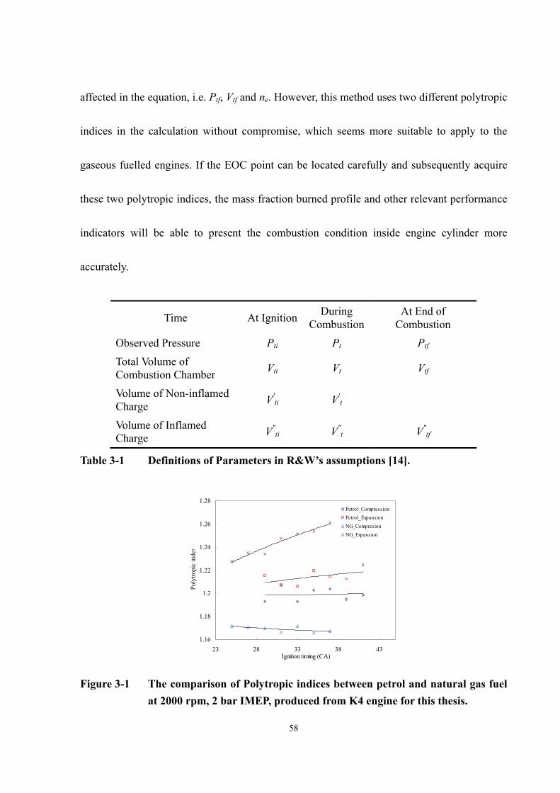
58

affected in the equation, i.e. Ptf, Vtf and ne. However, this method uses two different polytropic

indices in the calculation without compromise, which seems more suitable to apply to the

gaseous fuelled engines. If the EOC point can be located carefully and subsequently acquire

these two polytropic indices, the mass fraction burned profile and other relevant performance

indicators will be able to present the combustion condition inside engine cylinder more

accurately.

Time At Ignition During Combustion

At End of Combustion

Observed Pressure Pti Pt Ptf

Total Volume of Combustion Chamber Vti Vt Vtf

Volume of Non-inflamed Charge V′ti V′t

Volume of Inflamed Charge V″ti V″t V″tf

Table 3-1 Definitions of Parameters in R&W’s assumptions [14].

1.16

1.18

1.2

1.22

1.24

1.26

1.28

23 28 33 38 43Ignition timing (CA)

Poly

tropi

c in

dex

Petrol_CompressionPetrol_ExpansionNG_CompresionNG_Expansion

Figure 3-1 The comparison of Polytropic indices between petrol and natural gas fuel at 2000 rpm, 2 bar IMEP, produced from K4 engine for this thesis.

59

3.2. Method of Linear Changes of Polytropic Indices

An alternative method to continuing the use of the common R&W model when compression

and expansion polytropic indices are very different, i.e. more than 0.1 in this study, is the

introduction of a non-constant linear polytropic indices method. Since the compression

polytropic index is based on unburned charge and the expansion polytropic index is based on

burned mixture, the value of the polytropic index during the period between ignition timing

and EOC position, it seems reasonable to assume that the polytropic index value n(θi) varies

linearly from compression index (general 1.15) to expansion index (general 1.25) with

increasing crank angle. The application is outlined below:

( ) ( ) e ci c i s

e s

n nn nθ θ θθ θ −= + − × −

Eq. 3-5

( ) ( ) ( )( )

( )

11

in

ic i i

i

VP P P

V

θθ

θ θθ+

+

∆ = −

Eq. 3-6

( )' ic c

c

VP P

Vθ

∆ = ∆

Eq. 3-7

( ) ∑∑ ∆∆= e

s

i

scci PPx θ

θ

θ

θθ '' Eq. 3-8

nc and ne are obtained directly from the log P-log V diagram which are the slopes of

polytropic processes in the compression and expansion processes respectively. Subscript s

and e denote the start and end of combustion, θi is the crank angle during combustion. ∆Pc

60

is the pressure increment due to combustion in each crank angle interval. P, V are the

measured pressure and volume at crank angle θi, Vc is the clearance volume.

The basic thinking behind this method is trying to smooth the variation of polytropic index

during the combustion period. The commonly used polytropic index methods either

underestimate or overestimate the result in the ignition delay or burn duration periods,

therefore this blended method gradually simulates the performance of combustion from

unburned charge behaviour toward the burned charge behaviour according to the progress of

combustion (not practical). It might be able to improve the accuracy of results.

3.3. Finding the End of Combustion

Eq. 3-3 and Eq. 3-4 both reveal the necessity of an accurate EOC point. However, in R&W’s

method there is no detailed explanation of finding it, because the flame progress is monitored

by motion pictures, hence such information was obtained entirely from observation. Therefore,

the method of try and error is needed for locating the EOC point, at least for the initial

position. The calculation result has to be examined following the initial supposition, which

means a check on the last increment of pressure produced by combustion if it turns to zero or

negative value. In real time analysis, this method might be not practical and the iterations of

61

calculation will occasionally take a very long time to reach convergence. Instead of blindly

guessing the EOC, Reddy and co-worker [35] suggested using differential pressure data to

decide the end of combustion for a diesel engine, which seems to be a good method to provide

a proper starting point for approaching the correct EOC position. Nevertheless, the suggested

criterion for determining its location does not seem to be suitable for the natural gas fuelled

engine.

Eq. 3-4 does not calculate the pressure increment at each crank angle, so the method of

examining the final pressure increment cannot be applied. However, the common R&W form

Eq. 2-12 can be considered as a reference method to obtain the correct EOC and then provide

the result to Eq. 3-4 for final calculation. Because the measured pressure traces, 100 cycles in

most cases of this study, will be smoothed and then averaged into only one single cycle for

further calculation the consideration of noise and interference can be ignored. Consequently,

for those three methods for deciding EOC mentioned in Section 2.2.5, the first negative one is

adopted on the basis of time saving. The in-house program uses one crank angle increment to

approach the EOC, it starts with the initial value derived from the aforementioned differential

method until the preset criterion, which is the first pressure increment equal to or less than

zero has been met. Figure 3-2 shows the approaching traces in a normal engine operating

condition arbitrarily selected from tests conducted for this thesis. From the left to the right, the

62

upper part of the MFB curve gradually becomes an asymptote toward unity, which means the

EOC point has been progressively reached. A flow diagram of this method is presented in

Figure 3-3.

1.05

0.73

0.75

0.80

0.85

0.90

0.95

1.00

420384 390 395 400 405 410 415

MFB(100%)

CA degree

Figure 3-2 The upper part of mass fraction burned profile, the traces fro the left to the right gradually approach to the final EOC position with one crank angle degree increment.

63

Figure 3-3 Flow diagram of the EOC approaching process.

64

3.4. Determination of the Polytropic Index

According to the discussion in the literature survey, there are many polytropic index methods

that have been used by researchers to calculate the mass fraction burned. The program

provides a selection knob for choosing between different polytropic index methods, five

options are available to choose.

(1) Compression –use compression index for the whole combustion period

(2) Linear – the index value varies from compression index to expansion index linearly

(3) Averaged – use the averaged value of two indices for calculation

(4) Switching – compression index is used before TDC, then switches to expansion

index for the remainder

(5) R&W method – both indices are used in calculation

Option 5 uses Eq. 3-4 and option 2 uses Eq. 3-5 ~ Eq. 3-8, the rest of methods use Eq. 2-12 to

calculate the MFB.

The most right term ( ) ( ) ( )1 ini iV V

θθ θ + in Eq. 3-6 determines the pressure increment of

each interval. When different polytropic index methods are applied on the same data, at the

same crank angle, the larger the value of this term, the smaller the increment will be. Figure

3-4 presents the effects of different polytropic index values on the results. Except the

compression index method, the effects are similar for the other three methods before TDC.

65

Differences begin from 5° CA ATDC, the value deduced by the linear index method varies

from averaged to switching index method. This phenomenon can be explained by

characteristic of the linear index method, which gradually increases the polytropic index from

compression to expansion value (same value used after TDC with the switching index

method).

It is known that under a polytropic process, a straight line should be found from a logarithmic

P-V diagram, however, the pressure data collected from engine are discrete points between

each resolution interval, a trend line needs to be found to represent the polytropic curve.

Because of the variations of combustion and random noises, even after data smoothing and

averaging, some points might still be apart from the trend line, hence it is necessary to use a

curve fitting method to obtain the regression line and slope, e.g. polytropic index. Previous

discussion has suggested that the linear least squares method is the most suitable strategy to

use, therefore, a best fit mechanism is adopted in the program to obtain the regression line

from those discrete data.

Since the slope is derived from the regression line, choosing the proper crank angle range

becomes critical. Normally, from the intake valve close (IVC) to ignition and from the end of

combustion to exhaust valve open (EVO) are both thought as appropriate periods of

examining the polytropic processes [26]. However, owing to the engine running condition

66

continually varying, shorter periods will be considered as more suitable.

3.4.1. Compression and Expansion Polytropic Index

The intake valve of the K4 engine closes at 52° CA after bottom dead centre, therefore, 290°

CA is chosen arbitrarily as a start point for calculating the compression polytropic index.

From the start point to ignition, i.e. MBT timing (31° CA BTDC for 2000 rpm, 2 bar IMEP

condition in this study), is about 40° CA, therefore it should be able to produce an adequate

trend line to predict the polytropic behaviour during the compression stroke.

The exhaust valve open at 52° CA BBDC, hence the end of examining period for the

expansion polytropic index is arbitrary set at 470° CA, about 20° CA before the valve opens.

The start position is from the calculated end of combustion point by the aforementioned

method. Owing to the temperature in the expansion stroke being higher than in the

compression stroke, causing greater heat transfer, the expansion polytropic index value is

normally larger than the compression value. Figure 3-5 shows how the program derives

polytropic indices from those four relevant points. Through this method, consequently, the

mass fraction burned calculation can now be conducted even more precisely.

67

0.96

0.97

0.98

0.99

1.00

1.01

1.02

1.03

1.04

329 349 369 389 409CA degree

[V(θ

i)/V(θi

+1)]^

n(θi

)

SwitchingLinearAveragedCompress

Figure 3-4 Effects of different polytropic index methods on deciding the pressure increment of K4 engine

Figure 3-5 log P – log V diagram in normal firing condition; the polytropic indices nc and ne in compression and expansion strokes respectively are derived by the best fit curve fitting.

68

3.5. Ignition Delay and Burn Duration

3.5.1. Ignition Delay

Some researchers investigated the diverge point from the pressure trace and defined the period

from the ignition to this diverge point as a delay period. In Heywood’s book [11], ignition

delay of spark ignition engine is called ‘flame-development angle’, it is the crank angle

interval between the spark ignition and a small amount of fuel energy having been released, or

a small but significant fraction of charge mass having been burned. For the mass fraction

burned, from 1% ~ 5% and 10% have all at times been used to define the ignition delay, 5% is

chosen arbitrarily in this study for convenience.

The ignition delay changes with equivalence ratio, spark timing and residual fraction. Sher

and Hacohen [94] defined the aforementioned departure point by d2p/dθ2 = 0 and said this

point normally corresponds to 2% MFB for a gasoline SI engine, this value will be examined

with regard to experimental results to see if it is still adequate when applied to natural gas fuel.

The ‘Turbulent entrainment model’ presented by Tabaczynski and co-workers [95] correlates

the ignition delay to the laminar flame speed, which is one of the disadvantages of using

natural gas fuel, therefore the ignition delay of a natural gas fuelled engine is supposed to be

longer than the traditional fuelled engine. Fortunately, this can be improved by adding

69

additives, e.g. hydrogen. The burning velocity of hydrogen is about 300 cm/s, which is eight

times more than normal hydrocarbon fuel. A more chemical way to illustrate the improvement

of ignition delay by the adding hydrogen was presented by Hassaneen and co-workers [40],

they concluded the ignition delay time depends on the rate of chemical processes in the

expanding flame kernel, adding hydrogen will accelerate the early stage of the combustion by

the rapid chain branching oxidation characteristics of hydrogen. Again, this accelerating

phenomenon will be examined by the durations of 5% MFB with different amount of

hydrogen additive.

3.5.2. Burn Duration

The rapid-burning angle, again by Heywood’s definition, of the SI engine is between the

ignition delay and 90% or 95% MFB empirically. The reason for not choosing the EOC as a

finish point is because of the difficulty of finding it, and the error can be minimized if one

overestimates this point (after real EOC CA, the increment of pressure by combustion should

be zero to the next combustion). Most researchers believe this period is controlled by the

turbulent transport, and the flame speed is increased approximately linearly with the engine

speed.

There are two alternative opinions with regard to the effect of hydrogen on this interval. Hires

70

and co-workers [96] said it will be reduced because of the faster laminar flame speed of

hydrogen. Blizard and Keck [97] proposed that the rate of turbulent flame propagation is

primarily governed by hydrodynamic processes during intake, compression and combustion,

therefore the addition of hydrogen is not very significant to the burn duration. The observation

here will focus on the interval change after adding hydrogen, and on examining the accuracy

of the proposed method of finding the EOC point by inspecting the trend consistence of 95%

MFB and the total combustion duration.

3.5.3. MFB Definitions Used in the Program

5% and 95% of MFB have been chosen in the program as end points of ignition delay and

burn duration respectively. The definitions of both terms are:

Ignition delay: ignition point ~ 5% MFB

Burn duration: 5 ~ 95% MFB

71

4. DESCRIPTION OF EXPERIMENTAL METHOD AND PROCEDURE

4.1. Hardware Arrangement

4.1.1. Engine

The single cylinder engine, called “K4 Medusa”, used in this study was effectively one

quartered from a Rover K16 1.8 litre 4 cylinder gasoline engine. Stone’s group [1, 53] has

used a similar design but with optical access at the University of Oxford for combustion and

cycle-by-cycle variation studies. Table 4-1 shows the specifications of the K4 engine.

Bore 80 mm Stroke 88.9 mm Displacement 446.86 cm3 Connecting-rod Length 160 mm Compression Ratio 10.5 : 1 Inlet Valve Opens 12 ﾟ BTDC Inlet Valve Closes 52 ﾟ ABDC Exhaust Valve Opens 52 ﾟ BBDC Exhaust Valve Closes 12 ﾟ ATDC

Table 4-1 Specifications of the K4 Medusa engine.

The original fuel injector is replaced by a gas carburettor so the gaseous fuels can be used.

Considering the high variation of intake air flow in single cylinder engine, the inlet air flow

rate is evaluated by a positive displacement rotary flow meter (Romet G40). After the flow

meter is a mixture throttle, which produces vacuum pressure in the mixture section to suck in

72

air and EGR. The other throttle is inside the carburettor, which controls the inlet mixture into

the engine by varying the throttle open area to adjust the inlet manifold pressure and create a

further vacuum in the mixture section. The amount of inlet air and fuel can be changed by

tuning these two throttles.

The spark plug is controlled by an engine control system IC5460 according with the TDC

signal from an optical shaft encoder (type: RS 341-581), which is coupled with the crank shaft

of the engine, detail specifications can be found in Table 4-2. The shaft encoder also supplies

degree signals (360 pulses per revolution) to trigger the data acquiring mechanism on a multi

I/O data acquisition card.

RS Stock Number 341-581 Pulses per revolution 360 Pulses Phase shift between A and B outputs 90 Degrees

High level 2.4 V Output signal A & B

Low level 0.4 V High level 2.4 V

Synch. Pulse output Low level 0.4 V

Operation frequency 50 kHz Equivalent disc speed 8333 rpm

Table 4-2 Specification of optical shaft encoder.

73

4.1.2. Fuel Supply

Natural gas fuel came directly from the mains gas, a pressure regulator reduced the pressure

to about 16 ~ 20 mbar and an automatic cut-off solenoid valve was installed for safety,

controlled by a tachometer set to monitor engine speed. A mains gas sample was sent to the

laboratory of Scienco Ltd. Birmingham for major components analysis in the early stage of

tests, the following compositions result was from their analysis report:

CH4 C2H6 C3H8 CO2 N2

84.5% 6.0% 1.5% 2.0% 6.0%

Table 4-3 Main compositions of natural gas used in the tests.

Consequently the molar weight of natural gas used in this study is 18.583 (kg/kmol). In

stoichiometric condition without considering dissociation, the chemical equilibrium equation

can be presented as

( )4 2 6 3 8 2 2 2 2

2 2 2

0.845CH 0.06C H 0.015C H 0.02CO 0.06N 1.975 O 3.76N1.93H O 1.03CO 7.49N

+ + + + + +→ + +

Eq. 4-1

The stoichiometric air/fuel ratio (λ) is 14.59 and CO2 is about 10 (wet) or 12 (dry) volume

percent in the exhaust. Except the nearly zero content of oxygen in the exhaust, the average

CO2 percentage (11%) in the emissions was occasionally adopted as an alternative criterion of

stoichiometric when the λ value indicated by the Horiba did not work properly.

74

An EGR loop was taken from the exhaust pipe 10 cm after the outlet port of engine, the

amount of EGR returning back to the engine intake system was controlled by a globe valve

sitting in the downstream section of the loop. The loop pipe, without any covering of

insulation material, will naturally cool down the temperature of exhaust gas before it joining

the inlet air. Hydrogen was stored in a high pressure vessel and mixed with natural gas fuel

before feeding into the gas carburettor. Figure 4-1 shows the detail intake piping system

arrangement.

4.1.3. Temperature Monitoring

Seven positions around the engine system have been monitored by K type thermocouples, all

the wires are connected to a multifunction meter, so the temperature of each position can be

read from the indicator by choosing the corresponding connection port. Table 4-4 lists the

relevant information.

Mark T1 T2 T3 T4 T5 T6 T7 Correspondent connection port 10 2 3 4 5 6 7

Description coolant in

coolant out oil in oil

out inlet

manifold exhaust

out air in

Table 4-4 List of temperature monitoring points.

The coolant and oil temperatures were kept at 90°C and 80°C respectively throughout the

75

engine testing period. All temperatures were recorded by the end of each test for future

analysis.

4.1.4. Emissions Measurement

An emissions analysis kit built up previously was used to examine the exhaust results during

the experiments. Three main emission items, i.e. CO, UHC, NO, and two combustion related

gases, e.g. CO2 and O2, were monitored and recorded for each test. The employed instruments

include:

Instrument Name Maker / Model Analysed Gas

Emission Analyser Horiba /

MEXA-574GE O2, CO2, CO, UHC

Infrared Analyser Beckman / 864 CO2 NO/NOx Analyser Beckman / 951A NO/NOx

Table 4-5 Instruments list of emissions analysis.

To make sure a stable condition can be reached, all equipments were warmed-up at least one

hour before testing and the cooling system has to reach the default temperature, the

calibrations of emissions analysis kit by zero and span gases were done before the very first

test in every testing day. Exhaust gas was collected through an insulated pipe, which was

taken from the exhaust pipe about 30cm from the engine exhaust port, then passed into a

conditioning unit. After water separating procedure, dry exhaust gas was then analysed by

76

those instruments. The definition of EGR% adopted in this study is by the volumetric change

of carbon dioxide:

( )( )

2

2

EGR% 100inlet

exhaust

COCO

= × Eq. 4-2

(CO2)exhaust measured the content of CO2 from the exhaust pipe when EGR was applying;

(CO2)inlet was obtained from the inlet manifold as switching off EGR supply. Both values

were taken from the Horiba.

4.1.5. Data Acquisition Rig

The schematic arrangement of the integral data acquisition system is presented by Figure 4-2,

the details of each item are explained below.

4.1.5.1. Data Acquisition Board

To acquire the pressure against volume signals from K4 engine at high speed and in real time,

a multifunction I/O board from National Instruments was chosen. This PCI-MIO-16E-4 card

is suitable for PCI bus computers with analog input, analog output, digital I/O and timing I/O

functions. Those specifications related to test settings are listed below:

77

Model PCI-MIO-16E-4 Analog input

Number of channels Resolution Max. sampling rate Input coupling Max working voltage

16 single-ended or 8 differential 12 bits 500 kS/s DC Bipolar input range of ±5V

Digital trigger Compatibility Response Pulse width

TTL Rising or falling edge 10 ns Min.

Table 4-6 Relevant specifications of data acquisition board: NI PCI-MIO-16E-4.

This card was installed in a personal computer with an AMD K6-333 processor and Windows

98 platform. The data acquiring functions were software controlled by NI DAQ 6.6 software

together with the LabVIEW program.

4.1.5.2. Pressure and Crank Angle Acquiring Instruments

A Kistler quartz pressure sensor (Model 6125A) with TiN coating was flush mounted in the

cylinder head, signals were then sent to a Kistler Charge Amplifier (Model 5011) to convert

the charge yielded from the piezoelectric effect into a proportional voltage signal. There are

four settings on the charge amplifier that needed to be set:

78

Charge Amplifier T

(Transducer sensitivity)

S (mechanical

Scale)

LP (Low Pass

filter)

TC (Time

Constant) Kistler 5011 15 20 3 k HZ Short

Table 4-7 Settings for charge amplifier.

A dead weight calibration is needed for using the combination set-up of a pressure transducer

and a charge amplifier. Except the time constant being set to “long” for calibration, which is

suggested by the user’s manual, the parameters were kept the same. Four calibrations were

conducted before installing the pressure transducer into the cylinder head, calibration results

are presented in Figure 4-3 and an average value is adopted for ongoing using. A detailed

calibration spreadsheet can be found in Appendix A. Deposits were found on the piezoelectric

surface of transducer after a numbers of tests, therefore a regular check and re-calibration

(probably every 20 working hours) is recommended for reasons of accuracy.

The first two charge amplifier settings decide the range of output signal, which has to be

smaller than the limit of the input signal of the data acquisition board. Since the signal is of a

differential type, according to Table 4-6, the safe working range is within ±5V. Figure 4-3

shows the chosen settings have restricted the output voltage less than 2V when the estimated

maximum pressure (35 bars) was reached, this will protect the data acquisition system from

overloading.

A shaft encoder, as mentioned earlier, was securely coupled with the engine spindle. TDC

79

position is supposed to be consistent with the synchronous pulse signal (1pulse/revolution) in

order to identify each revolution of crank shaft. By dividing each two TDC period into 360

intervals and correlating them with relative pressure signals acquired by one crank angle base,

the data of pressure traces versus cylinder volume can be derived. For convenience sake, the

TDC signal has been set up as 70° before real TDC position in the control system, on the

flywheel there is a TDC mark used for calibration, the TDC signal of the shaft encoder was

synchronized with this point, consequently all the stored pressure data have to be shifted -70°

CA in terms of cylinder volume.

Dynamometer

K4Engine Exhaust out

Mixture PressureGauge

PositiveDisplacement

Flow Meter

Air Filter

EGR Loop

GasCarburettor

Air in

Mixture Throttle

Inlet ManifoldPressure Gauge

Shaft Encoder

Piezoelectric PressureTransducer

T7T5

T6

Emissionspick-up point

Natural GasH2

Solenoid Valve

Emissionspick-up point

Figure 4-1 Intake piping arrangement of K4 engine.

80

Figure 4-2 Schematic diagram of data acquisition rig.

y = 0.0531x - 0.1598

-0.5

0

0.5

1

1.5

2

0 5 10 15 20 25 30 35 40

Pressure (bar)

Vol

tage

(vol

t)

Calibration 1

Calibration 2

Calibration 3

Calibration 4

Figure 4-3 Dead weight calibration results of pressure transducer and charge amplifier set with the similar setting of charge amplifier in the tests.

81

4.2. Program Description

In this study, an in-house program has been developed with the purposes of acquiring and

processing engine pressure and volume data in real-time. This program is written using the

graphic language software LabVIEW 5.1, three main functions are included: data acquisition,

IMEP and mass fraction burned calculations. Each function can be performed alone or

cooperation with one or two other functions to obtain the desired results. Figure 4-4 shows the

links and purposes of these functions. Figure 4-5 presents a partial view of the program and

highlights some relevant items with simple explanations.

4.2.1. Data Acquisition

Signals from shaft encoder and pressure transducer are connected to the connectors of the data

acquisition board. The scanning frequency of the board was chosen to use degree signals from

the shaft encoder, thus at each degree the TTL pulse (output signal A or B) from the shaft

encoder will trigger the data acquisition board to acquire the incoming signals once. Item 2 in

Figure 4-5 will display the signals condition, a simple examination of acquired data can be

done by checking this window.

Engine speed and desired cycle number have to be input before starting, the program will stop

82

the acquiring procedure and move on to the next step when the required number of signal has

been reached.

4.2.2. IMEP Calculation

The desired value of IMEP needs to be input before starting, when the result falls within the

chosen range, the value of COVIMEP will show up and pause the program, this step will give

the tester a chance to decide whether to store the data and move to IMEP function or not. For

calculating the IMEP, the following procedures are then conducted in order:

(1) Verify the TDC signals from data to divide pressure signals into cycles

(2) Examine each set of cycle data and eliminate bad cycle(s) by judging whether there

are 720 signals in the cycle

(3) Correlate the pressure data with crank angle

(4) Smooth pressure data by chosen method. See item 5 in Figure 4-5

(5) Average all good cycles and convert pressure to absolute value by referring the inlet

manifold pressure as BDC pressure. See item 9 in Figure 4-5

(6) Correlate the average pressure with the cylinder volume

(7) Calculate the IMEP, COVIMEP and find out the maximum pressure in each cycle

The cylinder volume at crank angle θ is calculated by the following equations [11]:

83

2

4 2cB LV V l sπ = + + −

Eq. 4-3

12 2

2 2cos sin2 4L Ls lθ θ

= + −

Eq. 4-4

where Vc is the clearance volume, B is the cylinder bore diameter, l is the length of

connecting-rod and L is the stroke.

In this study, the compression ratio rc is 10.5, therefore Vc can be obtained by the

following equation:

1s

cc

VVr

=−

Eq. 4-5

where Vs is the swept volume of engine.

IMEP is calculated by Eq. 2-8 and COV is by Eq. 2-9. The detail calculation of IMEP can be

found in Appendix B.

4.2.3. Mass Fraction Burned

To investigate the combustion conditions, the results of mass fraction burned were used.

Through comparisons, a process obtained from selected methods mentioned in Chapter 3 will

be verified in Chapter 5 and adopted for further discussions. Both methods of finding the

initial EOC position and deriving the polytropic index value have to be chosen before starting,

they are item 7 and 4 respectively in Figure 4-5. The ignition timing of item 3 needs to be

84

input as well. The first and second differential pressure traces will not only be used to

estimate the initial EOC position, but also to predict the emissions behaviour, the detail will

be described in Chapter 7.

DataAcquisition

IMEPCalculation

Mass FractionBurned

Pressure Traces/

TDC Signals

Smoothed,AveragedAbsolute

Pressure vs.Volume

Saved RawData

Raw DataStorage

IMEP, Max.Pressure, COV

PolytropicIndex, MFB,

EOC,Differential

Pressure Data

Figure 4-4 Block diagram of three main functions in the program.

85

12

3

1

2

Main functions choosing buttons

Incoming signals monitoring window

Mass fraction burned set-up

6

8

4 Polytropic index method choosing knob

5 4 3

7

7

5

6

Data smoothing method

Scanning clock set-up

First EOC estimation method

8 Pressure signals calibration

9

9 Inlet manifold pressure

Figure 4-5 A partial front panel of the in-house program.

86

4.3. Test Procedure

Stoichiometric combustion is required to work successfully with a three-way catalyst in the

after-treatment of engine exhaust, typically the air/fuel ratio needs to be within 1% of the

stoichiometric value to protect the precious metals, hence such requirement will be adopted in

this study too. The drivability is another concern, to fulfil the stability requirement, COVIMEP

≤ 5% has been set as a basic criterion to make sure the cycle by cycle variations of IMEP will

not change too much.

Engine tests were conducted mainly by three base line operating conditions†, these tests

include some basic operating adjustments, i.e. engine speed, load and ignition timing, and will

establish a set of reference data for better understanding of some complex problems.

(1) Standard condition: 2000 rpm, 2 bar IMEP, -31° ATDC ignition timing‡,

stoichiometric condition and COVIMEP ≤ 5%.

(2) Higher load condition: 2000 rpm, 4bar IMEP, -31° ATDC ignition timing‡,

stoichiometric condition and COVIMEP ≤ 5%.

(3) Lower speed condition: 1500 rpm, 2 bar IMEP, -29° ATDC ignition timing‡,

stoichiometric condition and COVIMEP ≤ 5%.

† S, H and L may occasionally apply on some figures or captions to stand for above three operating conditions according to the order.

‡ Base line (MBT) timing, change of timing may be applied as condition required.

87

The following three investigations will be carried out and discussed individually.

(1) Since the revised r-R&W model has been selected for the MFB calculation,

consequently locating the EOC point and deducing two polytropic indices correctly

become significant. The most suitable data processing method for the present study

will be examined according to the results from above three operating conditions

(except the spark timing in lower speed condition has been advanced to 31° CA BTDC

for easy comparing). The chosen mechanism will then be secured and applied on all

the tests.

(2) Effects of additives on the combustion duration of a natural gas fuelled engine,

especially for adding EGR and hydrogen, will be investigated in terms of the

combustion indicators. A combined effect of EGR and hydrogen, based on the benefit

of exhaust gas reforming method, will then be examined and compared with the

individual effect. According to previous study, the volume percentage of EGR in the

inlet charge can be increased up to 25% with hydrogen as a supplement, the variations

of combustion durations during the change will be investigated by a gradually

increasing method, i.e. adding two additives alternately to extend the limit of EGR

content and still retain the COVIMEP under 5%.

(3) Taking emissions readings normally takes a number of actions to derive the results,

88

these have been found probably the most time consuming procedures in this study.

Therefore a simple measure that can reveal the tendency of the relevant emissions, i.e.

NO, CO, will be very efficient and attractive. The derivative of pressure data have

been found very useful in diagnosis of engine combustion, the first and second

derivative of pressure data will then be used as tools to investigate the relationships

with MFB profile and emissions behaviour. The object of this part is trying to predict

the required CA for each stage of MFB and the tendency of emissions within a

relevant window by using the differential pressure.

89

5. EFFECTS OF IMPROVED APPROACHES ON COMBUSTION DURATION

CALCULATION

Since the calculation of combustion duration in the present study is based on the incoming

signals indicating pressure and volume, the impacts on the result due to the data modifications

have to be examined before the further step of investigation the additives’ effects. However,

the combustion behaviours changes with changing engine operation, i.e. different ignition

timing, speeds and loads etc., have to be known in advance. Moreover, the phasing of pressure

in terms of crank angle needs to be accurate enough to calculate the IMEP and the data

smoothing methods should still retain the characteristics of combustion. This chapter will

explore the above issues and compare their effects using the MFB results calculated by the

revised R&W method (r-R&W), and then a decision should be made to select a more suitable

data processing method for natural gas fuelled engine. For the convenience of discussion, the

order of the following topics may not be consistent with the order of the program procedures.

However, the procedures of data analysis have already been outlined in Chapter 4.2.2.

5.1. Effects of Basic Operating Conditions

Cylinder combustion can be affected by many operating parameters, therefore this

90

investigation will only concentrate on these items related to the effects of adding EGR and (or)

hydrogen additive(s), they include engine speed, load (IMEP) and ignition timing.

5.1.1. Engine Speed

Two different speeds, i.e. 1500 and 2000 rpm were compared under similar operating

conditions. Data had not been modified by any smoothing methods (raw data), and the

switching polytropic index method was chosen arbitrarily to decide the EOC points. By using

the above data, the MFB results were then obtained using the r-R&W model.

Figure 5-1 shows MFB profiles of two different speeds at the same IMEP. The comparison, on

the basis of crank angles, reveals 25% more crank angle degrees are required to reach the first

5% MFB (ignition delay), however the time required at 2000 rpm is 6.3% less than at 1500

rpm. Higher speed takes less time and CA degrees during the burn duration (5% ~ 95% MFB),

which agrees with the explanation that the turbulence dominates the combustion speed during

this period and the engine speed has a direct link with the turbulence inside a cylinder.

Another phenomenon that should be noted is the proportion of combustion occurring prior to

TDC. To reach the same IMEP, with the same ignition timing, the lower speed condition

requires a greater percentage of mixture burned before 360° CA, thus more combustion

conducted in compression stroke. In this case, when the mass fraction burned was 12.3%

91

more conducted before TDC, it will cause a 40% higher average peak pressure in the

combustion.

5.1.2. Gross IMEP

According to Eq. 2-8, under a similar operating condition, higher IMEP requires higher

pressure to be produced inside the cylinder. The average peak pressures are 12 and 29.5 bar

with respect to 2 and 4 bars IMEP as shown in Figure 5-2 (A), this figure also shows the

pronounced pressure difference in terms of cylinder volume. In the 4 bar IMEP case, a steeper

pressure rise in the compression stroke after the ignition can be seen, probably because the

energy was released from more fuel mixture (76% more in this case), the other reason is the

percentage of burned gas occurring before TDC, 15% MFB difference has been observed.

Besides, in the 4 bars IMEP case, a longer total combustion period was needed, although the

95% MFB were indicating approximately the same in both tests.

5.1.3. Ignition Timing

Results in this section are derived from the data smoothed by the nine points weighted method,

EOC points were calculated through the switching polytropic index method and consequently

92

adopted for the revised R&W model in the MFB calculation.

Figure 5-3 shows the correlation between IMEP and ignition timing in three different

operating conditions. The MBT timing can be roughly located by finding the point on the

IMEP curve corresponding to the minimum point of the COVIMEP curve [98, Ch. 4], as a result

-31°, -29° and -31° are MBT timing for standard, lower speed and higher load conditions

respectively, ±1° tolerance should be considered because the test interval is 2° CA. Average

peak pressure decreased when the ignition timing moved toward TDC, there is no direct link

between peak pressure and IMEP value, although higher peak pressure do produce higher

IMEP, Figure 5-4 presents a linear-like relationship between average peak pressure and

ignition timing. Similar behaviour of NO in terms of ignition timing is also showing in this

diagram, such phenomena can be explained by the quantity of combustion occurring before

TDC. A retarded ignition will shorten the combustion time before TDC, therefore the pressure

and temperature inside cylinder decreases, and subsequently less NO will be produced in the

exhaust.

In standard condition, varying the ignition timing has been found to be irrelevant with regard

to the MFB profile, Figure 5-5 illustrates this phenomenon. It also provides a simple solution

to retaining a significant MFB value at a certain position without too much effort. Except in

the case of ignition timing 29° CA BTDC, an increasing combustion duration was concurrent

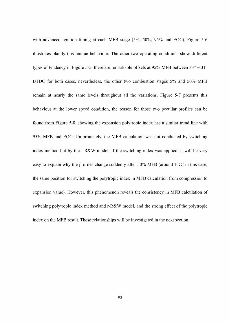
93

with advanced ignition timing at each MFB stage (5%, 50%, 95% and EOC), Figure 5-6

illustrates plainly this unique behaviour. The other two operating conditions show different

types of tendency in Figure 5-5, there are remarkable offsets at 95% MFB between 33° ~ 31°

BTDC for both cases, nevertheless, the other two combustion stages 5% and 50% MFB

remain at nearly the same levels throughout all the variations. Figure 5-7 presents this

behaviour at the lower speed condition, the reason for those two peculiar profiles can be

found from Figure 5-8, showing the expansion polytropic index has a similar trend line with

95% MFB and EOC. Unfortunately, the MFB calculation was not conducted by switching

index method but by the r-R&W model. If the switching index was applied, it will be very

easy to explain why the profiles change suddenly after 50% MFB (around TDC in this case,

the same position for switching the polytropic index in MFB calculation from compression to

expansion value). However, this phenomenon reveals the consistency in MFB calculation of

switching polytropic index method and r-R&W model, and the strong effect of the polytropic

index on the MFB result. These relationships will be investigated in the next section.

94

(A)

0

10

20

30

40

50

60

70

80

90

100

0 2 4 6 8 10Time (ms)

MFB

(%)

1500rpm

2000rpm

(B)

3600

10

20

30

40

50

60

70

80

90

100

329 349 369 389 409Crank angle (deg.)

MFB

(%)

1500rpm

2000rpm

Figure 5-1 The variation of MFB between two speeds at two different comparison bases, i.e. time and crank angle. Operating conditions: 2 bar IMEP, IG timing: -31° ATDC, COVIMEP ≤ 5 %.

(A)

0

5

10

15

20

25

30

0 100 200 300 400 500Volume (cm3)

Pres

sure

(bar

)

2 bar

4 bar

X ignition

+ EOC

O TDC

(B)

3600

10

20

30

40

50

60

70

80

90

100

329 349 369 389 409Crank angle (deg.)

MFB

(%)

2bar

4bar

Figure 5-2 Comparison between two different IMEP at 2000 rpm, IG timing: -31° ATDC. (A) P-V diagram (B) MFB.

95

(A)

1.85

1.9

1.95

2

2.05

2.1

2.15

2.2

2.25

-39 -37 -35 -33 -31 -29 -27 -25 -23 -21Ignition timing (CA ATDC, deg.)

IMEP

(bar

)

0.5

0.6

0.7

0.8

0.9

1

1.1

1.2

1.3

1.4

1.5

CO

VIM

EP (%

)

S LH_COV L_COV

(B)

3.8

3.9

4

4.1

4.2

4.3

4.4

4.5

-39 -37 -35 -33 -31 -29 -27 -25 -23 -21Ignition timing (CA ATDC, deg.)

IMEP

(bar

)

0.6

0.7

0.8

0.9

1

1.1

1.2

1.3

1.4

1.5

CO

VIM

EP (%

)

HH_COV

Figure 5-3 Correlations between ignition timing, IMEP and COVIMEP (A) Standard

and Lower speed conditions, (B) Higher load condition.

9

14

19

24

29

34

-39 -37 -35 -33 -31 -29 -27 -25 -23 -21Ignition timing (CA ATDC, deg.)

Ave

rage

pea

k pr

essu

re (b

ar)

0

500

1000

1500

2000

2500

NO

(ppm

)

H_Ppeak S_Ppeak L_Ppeak H_NO S_NO L_NO

Figure 5-4 Correlation between ignition timing and average peak pressure in three

different operating conditions; the related NO content in exhaust is showing the same tendency.

96

0

20

40

60

80

100

120

-39 -37 -35 -33 -31 -29 -27 -25 -23 -21

Ignition timing (CA ATDC, deg.)

Cra

nk a

ngle

(deg

.)

H_95% MFB L_95% MFB S_95% MFBH_50% MFB L_50% MFB S_50% MFBH_5% MFB L_5% MFB S_5% MFB

Figure 5-5 Comparison of 5%, 50% and 95% MFB in three different conditions.

-10%

10%

30%

50%

70%

90%

110%

320 370 420 470Crank angle (degree)

MFB

37 BTDC35 BTDC33 BTDC31 BTDC27 BTDC25 BTDC29 BTDC

Figure 5-6 MFB profile vs. ignition timing in standard condition.

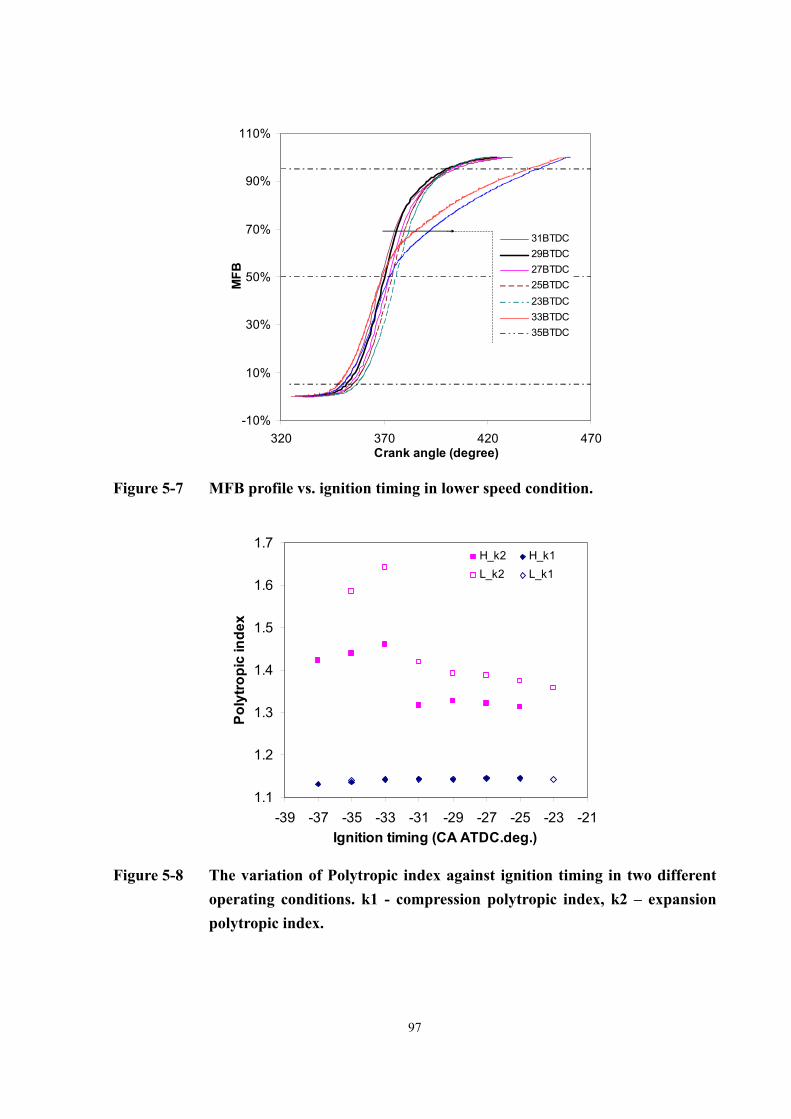
97

-10%

10%

30%

50%

70%

90%

110%

320 370 420 470Crank angle (degree)

MFB

31BTDC29BTDC27BTDC25BTDC23BTDC33BTDC35BTDC

Figure 5-7 MFB profile vs. ignition timing in lower speed condition.

1.1

1.2

1.3

1.4

1.5

1.6

1.7

-39 -37 -35 -33 -31 -29 -27 -25 -23 -21Ignition timing (CA ATDC.deg.)

Poly

tropi

c in

dex

H_k2 H_k1L_k2 L_k1

Figure 5-8 The variation of Polytropic index against ignition timing in two different

operating conditions. k1 - compression polytropic index, k2 – expansion polytropic index.

98

5.2. Effects of Data Processing and Analysis Methods

Data processing is necessary for data analysing, Figure 5-9 (A) illustrates one of the examples.

The diagram shows the improvement in the second derivative pressure data produced by

applying the low pass filter to the data. The derived data can then be used much more easily to

decide the initial EOC point and predict the emissions trend later. The disadvantage of

smoothing data is that the result may not be able to present the real condition if some

occasional abnormal phenomena are smoothed out. In this study, most of the data were taken

under acceptable drivability, i.e. COVIMEP ≤ 5%, which means that these unusual events had

already been exempted from the tests. Moreover, the stored computer files of satisfactory raw

data signals and piles of data sheets recorded with operating condition and emissions result

make it easy to reinvestigate.

Once engine speed, ignition timing and desired IMEP are decided, the calculation of duration

of combustion is determined by the accuracy of the data and the computation mechanism. If

any alteration has been done on raw data, the effect on the result needs to be evaluated and

borne in mind during the analysis. The in-house program introduces raw pressure signals into

the steps of phasing, pegging, smoothing and averaging before conducting the MFB

calculation, and the first three processing effects were investigated to help understand the

behaviour of the result.

99

5.2.1. Data Smoothing Methods

Due to unavoidable noise pickup and electronic interaction, data smoothing is necessary. Two

different methods were suggested above, they are the nine points weighted smoothing method

(9PWT, hereafter) as Eq. 2-4 and the low pass filter method (LPF, hereafter) as Eq. 2-5. Both

of them are believed to have superior performance for eliminating noise, and the latter has

also been claimed to show good performance on the second derivative of pressure data. Figure

5-9 (B) compares the second derivative of pressure data smoothed by the LPF and the 9PWS

methods; the former method does, in fact, present a better result. The average pressure cycle

is produced after the data smoothing procedure and used in MFB calculation to shorten the

time. The comparisons of MFB results between raw and smoothed data, which include the

individual and combined effects of these two smoothing methods, are discussed below.

5.2.2. Polytropic Index Method

There are many different polytropic index methods for mass fraction burned calculation. The

single value methods, it has been argued, tend to underestimate the results because a lower

index value is chosen in the expansion process. Therefore, the switching and linear methods

will be examined to see if they can provide more accurate results. The r-R&W method was set

100

up as a standard reference model to compare these differences.

Figure 5-10 to Figure 5-12 illustrate the MFB calculation results with different polytropic

index values when different smoothing methods were applied. Except in the Standard

condition, single index methods, i.e. compression and averaged polytropic index values, do

show shorter periods of combustion than the other two methods.

Four types of data condition were compared:

(A) Raw data – data derived from the data acquisition rig without a signal smoothing

procedure

(B) The LPF method

(C) The 9PWS method

(D) The combined method – signals smoothed by both LPF and 9PWS methods

In some cases, mostly when linear or switching polytropic index values were used, the total

combustion duration became very long. Therefore, the EOC point was too short to derive a

proper regression line, e.g. it was less than 10 CA degrees to the default end point (470 CA

degree) for deriving the expansion polytropic index value, so a further retarding action was

taken to extend the end point toward the exhaust valve opening crank angle (488 CA degree).

Those marked with the symbol * were in this condition.

Table 5-1 is related to Figure 5-10 ~ Figure 5-12 showing the differences in MFB results as

101

percentages under three engine operating conditions and using four different polytropic index

methods. There is no doubt that all the smoothed data delayed the calculation results of the

duration of total combustion. The worst cases happened when the LPF method was chosen,

whether it worked alone or was combined with the 9PWS method. A 65% increment (5.778

ms or 52° CA) of the total duration was found when either the linear or switching polytropic

index method was applied. An alternative method suggested by other researchers, which

decided the end of combustion by choosing a smaller value (95% in this study) of MFB was

found to make little improvement to the difference. However, up to 46.87% increment still

occurred when the switching method was used with LPF modified data. The nine points

weighted smoothing method worked adequately in all cases, especially in standard conditions,

and nearly the same results were found at 5%, 50% and 95% MFB calculations.

The compression polytropic index method produced very similar results with raw data no

matter what kind of smoothing mechanism was applied, which consequently makes the linear

and switching methods appear to overestimate the combustion duration, contradicting

previous research results. Nevertheless, a similar result with raw data does not guarantee the

accuracy, because the calculation according to the raw data could be wrong since it is

unfiltered, hence comparisons were made between different approaches and the reference

method, the r-R&W model.

102

Matrix structure comparisons originally stemming from Figure 5-10 ~ Figure 5-12 were

conducted and the results can be divided into three corresponding groups of diagrams: Figure

5-13 ~ Figure 5-16, Figure 5-17 ~ Figure 5-20 and Figure 5-21 ~ Figure 5-24. Each diagram

presents the difference in MFB profiles between the applied polytropic index method and the

r-R&W model, a table under the diagrams gives the percentage deviation at three combustion

stages. To use the r-R&W model for the MFB calculation, the EOC point has to be known in

advance; therefore in each comparison the EOC point derived from the other method was

used; thus both methods employ the same polytropic index value(s) and the combustion

finishes at the same point.

Figure 5-13 ~ Figure 5-16 illustrate the results originally from Figure 5-10 in the standard

operating condition. The switching index method has the best agreement with the r-R&W

model in all kinds of data, but the linear polytropic index method performed well too. A

slightly lower result from both single index methods was observed, as expected.

Figure 5-17 ~ Figure 5-20 are results initially from tests of Figure 5-11 in the higher load

condition. Pronounced deviations after 50% MFB happened in all cases; the low pass filter

smoothing worsens the results, as shown in Figure 5-18 and Figure 5-20. The nine points

weighted smoothing with the switching polytropic index method (9PWS-SW, hereafter) is

competent to produce a very similar profile to the r-R&W model; that is in response to the

103

previous discussion of data smoothing methods, which shows the potential of reliable

application.

Figure 5-21 ~ Figure 5-24 present comparisons in the lower speed condition than Figure 5-12.

Very similar comparison results were produced to the higher load condition, which

encourages the use of the 9PWS-SW mechanism. The linear polytropic index method does not

seem to be suitable for reconciling with those data smoothed by the lower pass filter method;

a gap during 60% ~ 90% MFB is obviously seen, and the deviation starts earlier than other

cases from TDC (about 30% MFB).

Compared with the other two operating conditions, the standard one shows less affected by

the chosen polytropic index method. Both dual index methods worked compatibly with each

other and show very close results to the r-R&W model, which encourages a further

investigation of the linear polytropic index method, because to the author’s knowledge, this

method has not been adopted by any other researcher. Since the 9PWS-SW mechanism has

shown potential for future use, the investigation of the effect of additives in the next chapter

will use this method for data processing in all cases.

5.2.3. Pressure Phasing

Although the TDC signal can be roughly calibrated before the experiment by observing the

104

motoring signals every time, there is still some possibility of phasing deviation, especially

when the engine is firing. During the experiments, the aluminium coupling connecting the

engine spindle and shaft encoder broke several times, due to the misalignment or high torque

rotation. When the fault occurred, the figure in the diagrams were twisted and deformed to

begin with, and then the data acquisition ceased to function because the checking mechanism

of the signal number could not reach the criteria in the program. Another defective condition

was that the TDC position deflected a few degrees away and the changes were hardly noticed.

Comparisons between correct phasing and degree offset error are discussed here. To simulate

the faulty condition, phasing from 1° CA to 5° CA and 10° CA advanced and retarded errors

are shown in Figure 5-25. In this test, the engine was run in standard operating condition, the

nine points weighted smoothing method was chosen to process the pressure data, the linear

polytropic index method was applied to decide the EOC point, and the MFB was derived by

the r-R&W model. Diagram (A) presents the MFB profile variations according to the phasing

errors; diagram (B) shows the trend lines of four combustion stages: 5%, 50%, 95% MFB and

EOC. The advanced and retarded phasing errors affected the 5% MFB calculation linearly; an

inclined tendency was observed from -10° CA to +10° CA. A dip area similar to the normal

heat transfer effect can be seen, owing to the retarded phasing; this phenomenon is

exaggerated when the phasing error increases. Conversely, the trends of 50%, 95% MFB and

105

EOC all incline from the advanced side down toward the retarded side. Such a result shortens

the period of burn duration but with a longer ignition delay, thus 12% increment of ignition

delay and a 22.7% reduction in burn duration were produced at a +5° CA phasing error.

Figure 5-26 presents the way in which the polytropic index values are affected by phasing

errors, the increasing compression index value k1 and the decreasing expansion index value

k2 correspond to the ignition delay and burn duration tendencies respectively.

In Figure 5-27, diagram (A), showing the effects on the IMEP and COVIMEP calculation, very

similar tendencies can be observed. The reason why the IMEP changes when the pressure

suffers phasing error can be easily explained by reference to diagram (B); that the deformed

compression and expansion strokes affect the IMEP calculation area can be seen.

There is a linear relationship between the percentage of IMEP inaccuracy and the phasing

error; only 5% IMEP deflection is observed in Figure 5-28 when the pressure with respect to

volume has 1° CA error; therefore, for the 2 bar IMEP test, setting up ± 0.1 bar as tolerance

value is within 1° CA phasing error. This result agrees with Figure 2-3 presented by Hribernik

[57].

5.2.4. Pressure Pegging

A piezoelectric transducer can only produce dynamic pressure data, but an absolute pressure

106

reference is needed for using such an instrument. According to the conclusions by [47-49], the

inlet manifold pressure was chosen because of its relevance. Pegging error normally occurs

when the reference datum is decided wrongly; such as when a wrong absolute pressure value

is given or the reference point is misplaced. The latter has been generally discussed in the

scope of phasing error; therefore the focus will be on the accuracy of the reference pressure.

Nevertheless, one should know that the pegging error will not affect either the IMEP result or

the COVIMEP, because the curve on the P-V diagram will simply be shifted vertically without

any deformation.

In the present test, the inlet manifold pressure value was obtained through a Bourdon gauge

and a sintered filter was fitted before the gauge in an attempt to attenuate the fluctuation

problem of the indicator. The reading was taken by eye measure and most of the readings

were decided by choosing the value from the middle of the variation range in a consequence

of the severe fluctuation. With increasing pegging value (absolute pressure of inlet manifold),

Figure 5-29 (A) shows that the MFB results gradually decreased, except that the 50% MFB

remained at the same level. 16% ignition delay reduction was caused by referencing a datum

with +0.2 bar absolute pressure error. Polytropic index values were affected, the compression

polytropic index k1 had similar behaviour as the ignition delay; this tendency is illustrated in

diagram (B).

107

(A)

-0.03

-0.02

-0.01

0

0.01

150 250 350 450 550Crank angle (deg.)

2nd

deriv

ativ

e of

pre

ssur

e da

ta

RawLPF

(B)

-0.03

-0.02

-0.01

0

0.01

150 250 350 450 550Crank angle (deg.)

2nd

deriv

ativ

e of

pre

ssur

e da

ta

9PWSLPF

Figure 5-9 The difference between raw data and smoothed data methods in 2nd derivative of pressure data in the standard operating condition. (A) Raw data vs. LPF, (B) 9PWS vs. LPF.

108

(A) Raw data

-10%

10%

30%

50%

70%

90%

110%

320 370 420 470Crank angle (degree)

MFB

Compress

Linear

Averaged

Sw itching

(B) Low pass filter

-10%

10%

30%

50%

70%

90%

110%

320 370 420 470Crank angle (degree)

MFB

(C) 9 points weighted smoothing

-10%

10%

30%

50%

70%

90%

110%

320 370 420 470Crank angle (degree)

MFB

(D) LPF + 9PWS

-10%

10%

30%

50%

70%

90%

110%

320 370 420 470Crank angle (degree)

MFB

(A)

5%MFB ms (CA)

50%MFB ms (CA)

95%MFB ms (CA)

Total ms (CA)

(B) 5%MFB ms (CA)

50%MFB ms (CA)

95%MFB ms (CA)

Total ms (CA)

Compress 2.000 (24) 3.750 (45) 5.167 (62) 5.917 (71) Compress 2.000 (24) 3.750 (45) 5.167 (62) 6.167 (74)

Linear 2.083 (25) 3.833 (46) 5.500 (66) 7.000 (84) Linear 2.083 (25) 3.917 (47) 5.583 (67) 7.500 (90)

Averaged 2.167 (26) 3.833 (46) 5.250 (63) 6.167 (74) Averaged 2.167 (26) 3.833 (46) 5.333 (64) 6.667 (80)

Switching 2.083 (25) 3.917 (47) 5.583 (67) 7.000 (84) Switching 2.083 (25) 3.917 (47) 5.667 (68) 7.500 (90)

(C) 5%MFB ms (CA)

50%MFB ms (CA)

95%MFB ms (CA)

Total ms (CA)

(D) 5%MFB ms (CA)

50%MFB ms (CA)

95%MFB ms (CA)

Total ms (CA)

Compress 2.000 (24) 3.750 (45) 5.167 (62) 6.083 (73) Compress 2.000 (24) 3.750 (45) 5.167 (62) 6.167 (74)

Linear 2.083 (25) 3.833 (46) 5.500 (66) 7.500 (90) Linear 2.083 (25) 3.917 (47) 5.583 (67) 7.500 (90)

Averaged 2.167 (26) 3.833 (46) 5.333 (64) 6.583 (79) Averaged 2.167 (26) 3.833 (46) 5.333 (64) 6.667 (80)

Switching 2.083 (25) 3.917 (47) 5.583 (67) 7.500 (90) Switching 2.083 (25) 3.917 (47) 5.667 (68) 7.500 (90)

Figure 5-10 The effects of data smoothing on MFB calculation results with different polytropic index methods. Engine operated in the standard condition.

109

(A) Raw data

-10%

10%

30%

50%

70%

90%

110%

320 370 420 470Crank angle (degree)

MFB

Compress

Linear

Averaged

Sw itching

(B) Low pass filter

-10%

10%

30%

50%

70%

90%

110%

320 370 420 470Crank angle (degree)

MFB

(C) 9 points weighted smoothing

-10%

10%

30%

50%

70%

90%

110%

320 370 420 470Crank angle (degree)

MFB

(D) LPF + 9PWS

-10%

10%

30%

50%

70%

90%

110%

320 370 420 470Crank angle (degree)

MFB

(A)

5%MFB ms (CA)

50%MFB ms (CA)

95%MFB ms (CA)

Total ms (CA)

(B) 5%MFB ms (CA)

50%MFB ms (CA)

95%MFB ms (CA)

Total ms (CA)

Compress 1.667 (20) 2.917 (35) 3.917 (47) 4.917 (59) Compress 1.667 (20) 2.917 (35) 4.000 (48) 5.000 (60)

Linear 1.750 (21) 3.000 (36) 4.917 (59) 7.667 (92) Linear* 1.750 (21) 3.083 (37) 7.083 (85) 11.333 (136)

Averaged 1.833 (22) 3.000 (36) 4.250 (51) 5.750 (69) Averaged 1.833 (22) 3.000 (36) 4.333 (52) 6.000 (72)

Switching 1.750 (21) 3.083 (37) 5.417 (65) 7.667 (92) Switching* 1.833 (22) 3.333 (40) 7.583 (91) 11.333 (136)

(C) 5%MFB ms (CA)

50%MFB ms (CA)

95%MFB ms (CA)

Total ms (CA)

(D) 5%MFB ms (CA)

50%MFB ms (CA)

95%MFB ms (CA)

Total ms (CA)

Compress 1.667 (20) 2.917 (35) 3.917 (47) 4.917 (59) Compress 1.667 (20) 2.917 (35) 4.000 (48) 5.000 (60)

Linear 1.750 (21) 3.000 (36) 4.833 (58) 8.583 (103) Linear* 1.750 (21) 3.083 (37) 6.333 (76) 11.250 (135)

Averaged 1.833 (22) 3.000 (36) 4.250 (51) 5.917 (71) Averaged 1.833 (22) 3.000 (36) 4.333 (52) 6.000 (72)

Switching 1.750 (21) 3.083 (37) 6.000 (68) 8.583 (103) Switching* 1.833 (22) 3.333 (40) 7.583 (91) 11.250 (135)

Figure 5-11 The effects of data smoothing on MFB calculation results with different polytropic index methods. Engine operated in higher load condition.

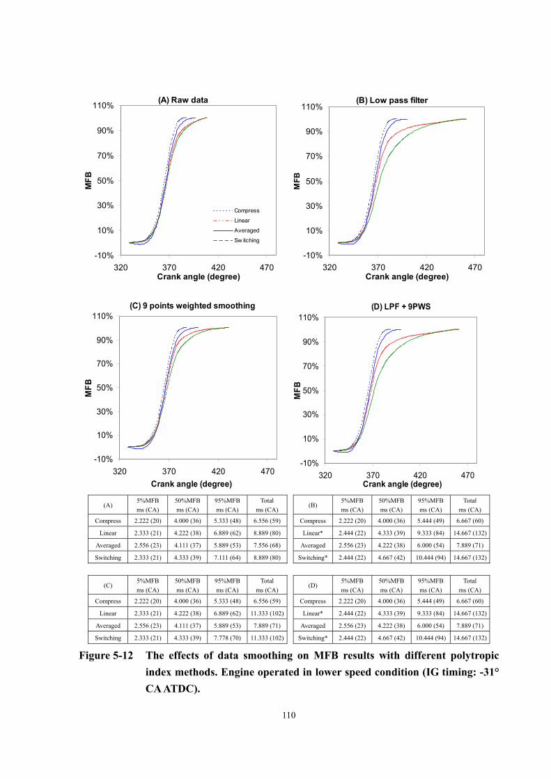
110

(A) Raw data

-10%

10%

30%

50%

70%

90%

110%

320 370 420 470Crank angle (degree)

MFB

Compress

Linear

Averaged

Sw itching

(B) Low pass filter

-10%

10%

30%

50%

70%

90%

110%

320 370 420 470Crank angle (degree)

MFB

(C) 9 points weighted smoothing

-10%

10%

30%

50%

70%

90%

110%

320 370 420 470Crank angle (degree)

MFB

(D) LPF + 9PWS

-10%

10%

30%

50%

70%

90%

110%

320 370 420 470Crank angle (degree)

MFB

(A)

5%MFB ms (CA)

50%MFB ms (CA)

95%MFB ms (CA)

Total ms (CA)

(B) 5%MFB ms (CA)

50%MFB ms (CA)

95%MFB ms (CA)

Total ms (CA)

Compress 2.222 (20) 4.000 (36) 5.333 (48) 6.556 (59) Compress 2.222 (20) 4.000 (36) 5.444 (49) 6.667 (60)

Linear 2.333 (21) 4.222 (38) 6.889 (62) 8.889 (80) Linear* 2.444 (22) 4.333 (39) 9.333 (84) 14.667 (132)

Averaged 2.556 (23) 4.111 (37) 5.889 (53) 7.556 (68) Averaged 2.556 (23) 4.222 (38) 6.000 (54) 7.889 (71)

Switching 2.333 (21) 4.333 (39) 7.111 (64) 8.889 (80) Switching* 2.444 (22) 4.667 (42) 10.444 (94) 14.667 (132)

(C) 5%MFB ms (CA)

50%MFB ms (CA)

95%MFB ms (CA)

Total ms (CA)

(D) 5%MFB ms (CA)

50%MFB ms (CA)

95%MFB ms (CA)

Total ms (CA)

Compress 2.222 (20) 4.000 (36) 5.333 (48) 6.556 (59) Compress 2.222 (20) 4.000 (36) 5.444 (49) 6.667 (60)

Linear 2.333 (21) 4.222 (38) 6.889 (62) 11.333 (102) Linear* 2.444 (22) 4.333 (39) 9.333 (84) 14.667 (132)

Averaged 2.556 (23) 4.111 (37) 5.889 (53) 7.889 (71) Averaged 2.556 (23) 4.222 (38) 6.000 (54) 7.889 (71)

Switching 2.333 (21) 4.333 (39) 7.778 (70) 11.333 (102) Switching* 2.444 (22) 4.667 (42) 10.444 (94) 14.667 (132)

Figure 5-12 The effects of data smoothing on MFB results with different polytropic index methods. Engine operated in lower speed condition (IG timing: -31° CA ATDC).

111

(1) Standard condition

(A) 5%MFB

ms (CA)

50%MFB

ms (CA)

95%MFB

ms(CA)

Total

ms (CA)

[(B) - (A)] / (A) 5%MFB 50%MFB 95%MFB Total

Compress 2.000 (24) 3.750 (45) 5.167 (62) 5.917 (71) Compress 0.00% 0.00% 0.00% 4.23%

Linear 2.083 (25) 3.833 (46) 5.500 (66) 7.000 (84) Linear 0.00% 2.19% 1.51% 7.14%

Averaged 2.167 (26) 3.833 (46) 5.250 (63) 6.167 (74) Averaged 0.00% 0.00% 1.58% 8.11%

Switching 2.083 (25) 3.917 (47) 5.583 (67) 7.000 (84) Switching 0.00% 0.00% 1.50% 7.14%

[(C) - (A)] / (A) 5%MFB 50%MFB 95%MFB Total

[(D) - (A)] / (A) 5%MFB 50%MFB 95%MFB Total

Compress 0.00% 0.00% 0.00% 2.81% Compress 0.00% 0.00% 0.00% 4.23%

Linear 0.00% 0.00% 0.00% 7.14% Linear 0.00% 2.19% 1.51% 7.14%

Averaged 0.00% 0.00% 1.58% 6.75% Averaged 0.00% 0.00% 1.58% 8.11%

Switching 0.00% 0.00% 0.00% 7.14% Switching 0.00% 0.00% 1.50% 7.14%

(2) Higher Load condition

(A) 5%MFB

ms (CA)

50%MFB

ms (CA)

95%MFB

ms(CA)

Total

ms (CA)

[(B) - (A)] /

(A) 5%MFB 50%MFB 95%MFB Total

Compress 1.667 (20) 2.917 (35) 3.917 (47) 4.917 (59) Compress 0.00% 0.00% 2.12% 1.69%

Linear 1.750 (21) 3.000 (36) 4.917 (59) 7.667 (92) Linear* 0.00% 2.77% 44.05% 47.82%

Averaged 1.833 (22) 3.000 (36) 4.250 (51) 5.750 (69) Averaged 0.00% 0.00% 1.95% 4.35%

Switching 1.750 (21) 3.083 (37) 5.417 (65) 7.667 (92) Switching* 4.74% 8.11% 39.99% 47.82%

[(C) - (A)] /

(A) 5%MFB 50%MFB 95%MFB Total

[(D) - (A)] / (A) 5%MFB 50%MFB 95%MFB Total

Compress 0.00% 0.00% 0.00% 0.00% Compress 0.00% 0.00% 2.12% 1.69%

Linear 0.00% 0.00% -1.71% 11.95% Linear* 0.00% 2.77% 28.80% 46.73%

Averaged 0.00% 0.00% 0.00% 2.90% Averaged 0.00% 0.00% 1.95% 4.35%

Switching 0.00% 0.00% 10.76% 11.95% Switching* 4.74% 8.11% 39.99% 46.73%

(3) Lower Speed condition (IG timing: -31° CA ATDC)

(A) 5%MFB

ms (CA)

50%MFB

ms (CA)

95%MFB

ms(CA)

Total

ms (CA)

[(B) - (A)] / (A) 5%MFB 50%MFB 95%MFB Total

Compress 2.222 (20) 4.000 (36) 5.333 (48) 6.556 (59) Compress 0.00% 0.00% 2.08% 1.69%

Linear 2.333 (21) 4.222 (38) 6.889 (62) 8.889 (80) Linear* 4.76% 2.63% 35.48% 65.00%

Averaged 2.556 (23) 4.111 (37) 5.889 (53) 7.556 (68) Averaged 0.00% 2.70% 1.88% 4.41%

Switching 2.333 (21) 4.333 (39) 7.111 (64) 8.889 (80) Switching* 4.76% 7.71% 46.87% 65.00%

[(C) - (A)] / (A) 5%MFB 50%MFB 95%MFB Total

[(D) - (A)] / (A) 5%MFB 50%MFB 95%MFB Total

Compress 0.00% 0.00% 0.00% 0.00% Compress 0.00% 0.00% 2.08% 1.69%

Linear 0.00% 0.00% 0.00% 27.49% Linear* 4.76% 2.63% 35.48% 65.00%

Averaged 0.00% 0.00% 0.00% 4.41% Averaged 0.00% 2.70% 1.88% 4.41%

Switching 0.00% 0.00% 9.38% 27.49% Switching* 4.76% 7.71% 46.87% 65.00%

Table 5-1 The differences of MFB calculation between raw and smoothed data under diferent operating conditions and polytropic index values.

112

(1)

-10%

10%

30%

50%

70%

90%

110%

320 370 420 470

Crank angle (degree)

MFB

Compressr-R&W

(2)

-10%

10%

30%

50%

70%

90%

110%

320 370 420 470

Crank angle (degree)

MFB

Linearr-R&W

(3)

-10%

10%

30%

50%

70%

90%

110%

320 370 420 470Crank angle (degree)

MFB

Aeragedr-R&W

(4)

-10%

10%

30%

50%

70%

90%

110%

320 370 420 470Crank angle (degree)

MFB

Switchingr-R&W

(1) 5%MFB ms (CA)

50%MFB ms (CA)

95%MFB ms (CA)

Total ms (CA)

(2) 5%MFB ms (CA)

50%MFB ms (CA)

95%MFB ms (CA)

Total ms (CA)

Compress 0.00% -4.26% -4.62% Linear 0.00% -2.13% -2.94%

r-R&W 2.000 (24) 3.917 (47) 5.417 (65) 5.917 (71)

r-R&W 2.083 (25) 3.917 (47) 5.667 (68) 7.000 (84)

(3) 5%MFB ms (CA)

50%MFB ms (CA)

95%MFB ms (CA)

Total ms (CA)

(4) 5%MFB ms (CA)

50%MFB ms (CA)

95%MFB ms (CA)

Total ms (CA)

Averaged 8.33% -2.13% -4.55% Switching 0.00% 0.00% -1.47%

r-R&W 2.000 (24) 3.917 (47) 5.500 (66) 6.167 (74)

r-R&W 2.083 (25) 3.917 (47) 5.667 (68) 7.000 (84)

Figure 5-13 The comparison of MFB results between different polytropic index methods and revised R&W model. Data smoothing method: raw data; engine operated in standard condition. Percentages stand for the deviation from the r-R&W model.

113

(1)

-10%

10%

30%

50%

70%

90%

110%

320 370 420 470

Crank angle (degree)

MFB

Compressr-R&W

(2)

-10%

10%

30%

50%

70%

90%

110%

320 370 420 470

Crank angle (degree)

MFB

Linearr-R&W

(3)

-10%

10%

30%

50%

70%

90%

110%

320 370 420 470Crank angle (degree)

MFB

Averagedr-R&W

(4)

-10%

10%

30%

50%

70%

90%

110%

320 370 420 470Crank angle (degree)

MFB

Switchingr-R&W

(1)

5%MFB ms (CA)

50%MFB ms (CA)

95%MFB ms (CA)

Total ms (CA)

(2) 5%MFB ms (CA)

50%MFB ms (CA)

95%MFB ms (CA)

Total ms (CA)

Compress -4.00% -4.26% -6.06% Linear 0.00% 0.00% -2.90%

r-R&W 2.083 (25) 3.917 (47) 5.500 (66) 6.167 (74)

r-R&W 2.083 (25) 3.917 (47) 5.750 (69) 7.500 (90)

(3) 5%MFB ms (CA)

50%MFB ms (CA)

95%MFB ms (CA)

Total ms (CA)

(4) 5%MFB ms (CA)

50%MFB ms (CA)

95%MFB ms (CA)

Total ms (CA)

Averaged 4.00% -2.13% -5.88% Switching 0.00% 0.00% -1.45%

r-R&W 2.083 (25) 3.917 (47) 5.667(68) 6.667 (80)

r-R&W 2.083 (25) 3.917 (47) 5.750 (69) 7.500 (90)

Figure 5-14 The comparison of MFB results between different polytropic index methods and revised R&W model. Data smoothing method: low pass filter; engine operated in standard condition. Percentages stand for the deviation from the r-R&W model.

114

(1)

-10%

10%

30%

50%

70%

90%

110%

320 370 420 470

Crank angle (degree)

MFB

Compressr-R&W

(2)

-10%

10%

30%

50%

70%

90%

110%

320 370 420 470

Crank angle (degree)

MFB

Linearr-R&W

(3)

-10%

10%

30%

50%

70%

90%

110%

320 370 420 470Crank angle (degree)

MFB

Averagedr-R&W

(4)

-10%

10%

30%

50%

70%

90%

110%

320 370 420 470Crank angle (degree)

MFB

Switchingr-R&W

(1) 5%MFB ms (CA)

50%MFB ms (CA)

95%MFB ms (CA)

Total ms (CA)

(2) 5%MFB ms (CA)

50%MFB ms (CA)

95%MFB ms (CA)

Total ms (CA)

Compress 0.00% -4.26% -4.62% Linear 0.00% -2.13% -4.35%)

r-R&W 2.000 (24) 3.917 (47) 5.417 (65) 6.083 (73)

r-R&W 2.083 (25) 3.917 (47) 5.750 (69) 7.500 (90)

(3) 5%MFB ms (CA)

50%MFB ms (CA)

95%MFB ms (CA)

Total ms (CA)

(4) 5%MFB ms (CA)

50%MFB ms (CA)

95%MFB ms (CA)

Total ms (CA)

Averaged 8.33% -2.13% -4.48% Switching 0.00% 0.00% -2.90%

r-R&W 2.000 (24) 3.917 (47) 5.583 (67) 6.583 (79)

r-R&W 2.083 (25) 3.917 (47) 5.750 (69) 7.500 (90)

Figure 5-15 The comparison of MFB results between different polytropic index methods and revised R&W model. Data smoothing method: 9 points weighted smoothing; engine operated in standard condition. Percentages stand for the deviation from the r-R&W model.

115

(1)

-10%

10%

30%

50%

70%

90%

110%

320 370 420 470

Crank angle (degree)

MFB

Compressr-R&W

(2)

-10%

10%

30%

50%

70%

90%

110%

320 370 420 470

Crank angle (degree)

MFB

Linearr-R&W

(3)

-10%

10%

30%

50%

70%

90%

110%

320 370 420 470Crank angle (degree)

MFB

Averagedr-R&W

(4)

-10%

10%

30%

50%

70%

90%

110%

320 370 420 470Crank angle (degree)

MFB

Switchingr-R&W

(1)

5%MFB ms (CA)

50%MFB ms (CA)

95%MFB ms (CA)

Total ms (CA)

(2) 5%MFB ms (CA)

50%MFB ms (CA)

95%MFB ms (CA)

Total ms (CA)

Compress -4.00% -4.26% -6.06% Linear 0.00% 0.00% -2.90%

r-R&W 2.083 (25) 3.917 (47) 5.500 (66) 6.167 (74)

r-R&W 2.083 (25) 3.917 (47) 5.750 (69) 7.500 (90)

(3) 5%MFB ms (CA)

50%MFB ms (CA)

95%MFB ms (CA)

Total ms (CA)

(4) 5%MFB ms (CA)

50%MFB ms (CA)

95%MFB ms (CA)

Total ms (CA)

Averaged 4.00% -2.13% -5.88% Switching 0.00% 0.00% -1.45%

r-R&W 2.083 (25) 3.917 (47) 5.667 (68) 6.667 (80)

r-R&W 2.083 (25) 3.917 (47) 5.750 (69) 7.500 (90)

Figure 5-16 The comparison of MFB results between different polytropic index methods and revised R&W model. Data smoothing method: LPF + 9PWS; engine operated in standard condition. Percentages stand for the deviation from the r-R&W model.

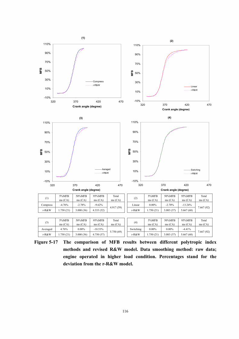
116

(1)

-10%

10%

30%

50%

70%

90%

110%

320 370 420 470

Crank angle (degree)

MFB

Compressr-R&W

(2)

-10%

10%

30%

50%

70%

90%

110%

320 370 420 470

Crank angle (degree)

MFB

Linearr-R&W

(3)

-10%

10%

30%

50%

70%

90%

110%

320 370 420 470Crank angle (degree)

MFB

Aeragedr-R&W

(4)

-10%

10%

30%

50%

70%

90%

110%

320 370 420 470

Crank angle (degree)

MFB

Swtchingr-R&W

(1)

5%MFB ms (CA)

50%MFB ms (CA)

95%MFB ms (CA)

Total ms (CA)

(2) 5%MFB ms (CA)

50%MFB ms (CA)

95%MFB ms (CA)

Total ms (CA)

Compress -4.76% -2.78% -9.62% Linear 0.00% -2.70% -13.24%

r-R&W 1.750 (21) 3.000 (36) 4.333 (52) 4.917 (59)

r-R&W 1.750 (21) 3.083 (37) 5.667 (68) 7.667 (92)

(3) 5%MFB ms (CA)

50%MFB ms (CA)

95%MFB ms (CA)

Total ms (CA)

(4) 5%MFB ms (CA)

50%MFB ms (CA)

95%MFB ms (CA)

Total ms (CA)

Averaged 4.76% 0.00% -10.53% Switching 0.00% 0.00% -4.41%

r-R&W 1.750 (21) 3.000 (36) 4.750 (57) 5.750 (69)

r-R&W 1.750 (21) 3.083 (37) 5.667 (68) 7.667 (92)

Figure 5-17 The comparison of MFB results between different polytropic index methods and revised R&W model. Data smoothing method: raw data; engine operated in higher load condition. Percentages stand for the deviation from the r-R&W model.

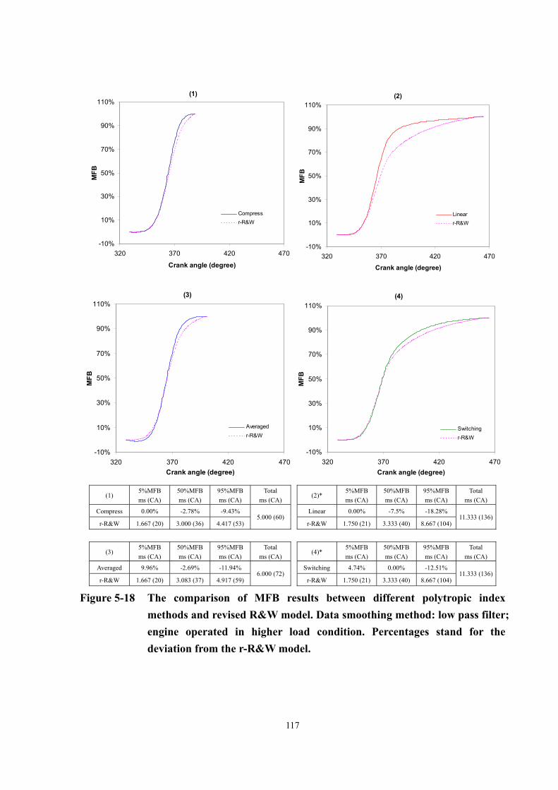
117

(1)

-10%

10%

30%

50%

70%

90%

110%

320 370 420 470

Crank angle (degree)

MFB

Compressr-R&W

(2)

-10%

10%

30%

50%

70%

90%

110%

320 370 420 470

Crank angle (degree)

MFB

Linearr-R&W

(3)

-10%

10%

30%

50%

70%

90%

110%

320 370 420 470Crank angle (degree)

MFB

Averagedr-R&W

(4)

-10%

10%

30%

50%

70%

90%

110%

320 370 420 470Crank angle (degree)

MFB

Switchingr-R&W

(1)

5%MFB ms (CA)

50%MFB ms (CA)

95%MFB ms (CA)

Total ms (CA)

(2)* 5%MFB ms (CA)

50%MFB ms (CA)

95%MFB ms (CA)

Total ms (CA)

Compress 0.00% -2.78% -9.43% Linear 0.00% -7.5% -18.28%

r-R&W 1.667 (20) 3.000 (36) 4.417 (53) 5.000 (60)

r-R&W 1.750 (21) 3.333 (40) 8.667 (104) 11.333 (136)

(3) 5%MFB ms (CA)

50%MFB ms (CA)

95%MFB ms (CA)

Total ms (CA)

(4)* 5%MFB ms (CA)

50%MFB ms (CA)

95%MFB ms (CA)

Total ms (CA)

Averaged 9.96% -2.69% -11.94% Switching 4.74% 0.00% -12.51%

r-R&W 1.667 (20) 3.083 (37) 4.917 (59) 6.000 (72)

r-R&W 1.750 (21) 3.333 (40) 8.667 (104) 11.333 (136)

Figure 5-18 The comparison of MFB results between different polytropic index methods and revised R&W model. Data smoothing method: low pass filter; engine operated in higher load condition. Percentages stand for the deviation from the r-R&W model.

118

(1)

-10%

10%

30%

50%

70%

90%

110%

320 370 420 470Crank angle (degree)

MFB

Compressr-R&W

(2)

-10%

10%

30%

50%

70%

90%

110%

320 370 420 470

Crank angle (degree)M

FB

Linearr-R&W

(3)

-10%

10%

30%

50%

70%

90%

110%

320 370 420 470Crank angle (degree)

MFB

Averagedr-R&W

(4)

-10%

10%

30%

50%

70%

90%

110%

320 370 420 470Crank angle (degree)

MFB

Switchingr-R&W

(1) 5%MFB ms (CA)

50%MFB ms (CA)

95%MFB ms (CA)

Total ms (CA)

(2) 5%MFB ms (CA)

50%MFB ms (CA)

95%MFB ms (CA)

Total ms (CA)

Compress 0.00% -2.78% -9.62% Linear 0.00% -2.70% -19.44%

r-R&W 1.667 (20) 3.000 (36) 4.333 (52) 4.917 (59)

r-R&W 1.750 (21) 3.083 (37) 6.000 (72) 8.583 (103)

(3) 5%MFB ms (CA)

50%MFB ms (CA)

95%MFB ms (CA)

Total ms (CA)

(4) 5%MFB ms (CA)

50%MFB ms (CA)

95%MFB ms (CA)

Total ms (CA)

Averaged 4.76% 0.00% -12.07% Switching 0.00% 0.00% -5.56%

r-R&W 1.750 (21) 3.000 (36) 4.833 (58) 5.917 (71)

r-R&W 1.750 (21) 3.083 (37) 6.000 (72) 8.583 (103)

Figure 5-19 The comparison of MFB results between different polytropic index methods and revised R&W model. Data smoothing method: 9 points weighted smoothing; engine operated in higher load condition. Percentages stand for the deviation from the r-R&W model.

119

(1)

-10%

10%

30%

50%

70%

90%

110%

320 370 420 470

Crank angle (degree)

MFB

Compressr-R&W

(2)

-10%

10%

30%

50%

70%

90%

110%

320 370 420 470

Crank angle (degree)

MFB

Linearr-R&W

(3)

-10%

10%

30%

50%

70%

90%

110%

320 370 420 470Crank angle (degree)

MFB

Averagedr-R&W

(4)

-10%

10%

30%

50%

70%

90%

110%

320 370 420 470Crank angle (degree)

MFB

Switchingr-R&W

(1)

5%MFB ms (CA)

50%MFB ms (CA)

95%MFB ms (CA)

Total ms (CA)

(2)* 5%MFB ms (CA)

50%MFB ms (CA)

95%MFB ms (CA)

Total ms (CA)

Compress 0.00% -2.78% 9.43% Linear 0.00% -9.76% -30.28%

r- R&W 1.667 (20) 3.000 (36) 4.417 (53) 5.000 (60)

r-R&W 1.750 (21) 3.417 (41) 9.083 (109) 11.250 (135)

(3) 5%MFB ms (CA)

50%MFB ms (CA)

95%MFB ms (CA)

Total ms (CA)

(4)* 5%MFB ms (CA)

50%MFB ms (CA)

95%MFB ms (CA)

Total ms (CA)

Averaged 10.00% -2.70% -11.86% Switching 4.76% -2.44% -16.51%

r-R&W 1.667 (20) 3.083 (37) 4.917 (59) 6.000 (72)

r-R&W 1.750 (21) 3.417 (41) 9.083 (109) 11.250 (135)

Figure 5-20 The comparison of MFB results between different polytropic index methods and revised R&W model. Data smoothing method: LPF + 9PWS; engine operated in higher load condition. Percentages stand for the deviation from the r-R&W model.

120

(1)

-10%

10%

30%

50%

70%

90%

110%

320 370 420 470

Crank angle (degree)

MFB

Compressr-R&W

(2)

-10%

10%

30%

50%

70%

90%

110%

320 370 420 470

Crank angle (degree)

MFB

Linearr-R&W

(3)

-10%

10%

30%

50%

70%

90%

110%

320 370 420 470Crank angle (degree)

MFB

Averagedr-R&W

(4)

-10%

10%

30%

50%

70%

90%

110%

320 370 420 470Crank angle (degree)

MFB

Switchingr-R&W

(1)

5%MFB ms (CA)

50%MFB ms (CA)

95%MFB ms (CA)

Total ms (CA)

(2) 5%MFB ms (CA)

50%MFB ms (CA)

95%MFB ms (CA)

Total ms (CA)

Compress 0.00% -2.70% -9.43% Linear 5.00% -2.56% -6.06%

r-R&W 2.222 (20) 4.111 (37) 5.889 (53) 6.556 (59)

r-R&W 2.222 (20) 4.333 (39) 7.333 (66) 8.889 (80)

(3) 5%MFB ms (CA)

50%MFB ms (CA)

95%MFB ms (CA)

Total ms (CA)

(4) 5%MFB ms (CA)

50%MFB ms (CA)

95%MFB ms (CA)

Total ms (CA)

Averaged 15.00% -2.63% -10.17% Switching 5.00% 0.00% -3.03%

r-R&W 2.222 (20) 4.222 (38) 6.556 (59) 7.556 (68)

r-R&W 2.222 (20) 4.333 (39) 7.333 (66) 8.889 (80)

Figure 5-21 The comparison of MFB results between different polytropic index methods and revised R&W model. Data smoothing method: raw data; engine operated in lower speed condition (IG timing: -31° CA ATDC). Percentages stand for the deviation from the r-R&W model.

121

(1)

-10%

10%

30%

50%

70%

90%

110%

320 370 420 470

Crank angle (degree)

MFB

Compressr-R&W

(2)

-10%

10%

30%

50%

70%

90%

110%

320 370 420 470

Crank angle (degree)

MFB

Linearr-R&W

(3)

-10%

10%

30%

50%

70%

90%

110%

320 370 420 470Crank angle (degree)

MFB

Averagedr-R&W

(4)

-10%

10%

30%

50%

70%

90%

110%

320 370 420 470Crank angle (degree)

MFB

Switchingr-R&W

(1)

5%MFB ms (CA)

50%MFB ms (CA)

95%MFB ms (CA)

Total ms (CA)

(2)* 5%MFB ms (CA)

50%MFB ms (CA)

95%MFB ms (CA)

Total ms (CA)

Compress 0.00% -2.70% -9.26% Linear 4.76% -9.30% -22.94%

r-R&W 2.222 (20) 4.111 (37) 6.000 (54) 6.667 (60)

r-R&W 2.333 (21) 4.778 (43) 12.111 (109) 14.667 (132)

(3) 5%MFB ms (CA)

50%MFB ms (CA)

95%MFB ms (CA)

Total ms (CA)

(4)* 5%MFB ms (CA)

50%MFB ms (CA)

95%MFB ms (CA)

Total ms (CA)

Averaged 15.00% 0.00% -11.48% Switching 4.76% -2.33% -13.76%

r-R&W 2.222 (20) 4.222 (38) 6.778 (61) 7.889 (71)

r-R&W 2.333 (21) 4.778 (43) 12.111 (109) 14.667 (132)

Figure 5-22 The comparison of MFB results between different polytropic index methods and revised R&W model. Data smoothing method: low pass filter; engine operated in lower speed condition (IG timing: -31° CA ATDC). Percentages stand for the deviation from the r-R&W model.

122

(1)

-10%

10%

30%

50%

70%

90%

110%

320 370 420 470

Crank angle (degree)

MFB

Compressr-R&W

(2)

-10%

10%

30%

50%

70%

90%

110%

320 370 420 470

Crank angle (degree)

MFB

Linearr-R&W

(3)

-10%

10%

30%

50%

70%

90%

110%

320 370 420 470Crank angle (degree)

MFB

Averagedr-R&W

(4)

-10%

10%

30%

50%

70%

90%

110%

320 370 420 470Crank angle (degree)

MFB

Switchingr-R&W

(1)

5%MFB ms (CA)

50%MFB ms (CA)

95%MFB ms (CA)

Total ms (CA)

(2) 5%MFB ms (CA)

50%MFB ms (CA)

95%MFB ms (CA)

Total ms (CA)

Compress 0.00% -2.70% -9.43% Linear 0.00% -2.56% -17.33%

r-R&W 2.222 (20) 4.111 (37) 5.889 (53) 6.556 (59)

r-R&W 2.333 (21) 4.333 (39) 8.333 (75) 11.333 (102)

(3) 5%MFB ms (CA)

50%MFB ms (CA)

95%MFB ms (CA)

Total ms (CA)

(4) 5%MFB ms (CA)

50%MFB ms (CA)

95%MFB ms (CA)

Total ms (CA)

Averaged 15.0% -2.63% -11.67% Switching 0.00% 0.00% -6.67%

r-R&W 2.222 (20) 4.222 (38) 6.667 (60) 7.889 (71)

r-R&W 2.333 (21) 4.333 (39) 8.333 (75) 11.333 (102)

Figure 5-23 The comparison of MFB results between different polytropic index methods and revised R&W model. Data smoothing method: 9 points weighted smoothing; engine operated in lower speed condition (IG timing: -31° CA ATDC). Percentages stand for the deviation from the r-R&W model.

123

(1)

-10%

10%

30%

50%

70%

90%

110%

320 370 420 470

Crank angle (degree)

MFB

Compressr-R&W

(2)

-10%

10%

30%

50%

70%

90%

110%

320 370 420 470

Crank angle (degree)

MFB

Linearr-R&W

(3)

-10%

10%

30%

50%

70%

90%

110%

320 370 420 470Crank angle (degree)

MFB

Averagedr-R&W

(4)

-10%

10%

30%

50%

70%

90%

110%

320 370 420 470Crank angle (degree)

MFB

Switchingr-R&W

(1)

5%MFB ms (CA)

50%MFB ms (CA)

95%MFB ms (CA)

Total ms (CA)

(2)* 5%MFB ms (CA)

50%MFB ms (CA)

95%MFB ms (CA)

Total ms (CA)

Compress 0.00% -2.70% -9.26% Linear 4.76% -9.30% -22.94%

r-R&W 2.222 (20) 4.111 (37) 6.000 (54) 6.667 (60)

r-R&W 2.333 (21) 4.778 (43) 12.111 (109) 14.667 (132)

(3) 5%MFB ms (CA)

50%MFB ms (CA)

95%MFB ms (CA)

Total ms (CA)

(4)* 5%MFB ms (CA)

50%MFB ms (CA)

95%MFB ms (CA)

Total ms (CA)

Averaged 15.00% 0.00% -11.48% Switching 4.76% -2.33% -13.76%

r-R&W 2.222 (20) 4.222 (38) 6.778 (61) 7.889 (71)

r-R&W 2.333 (21) 4.778 (43) 12.111 (109) 14.667 (132)

Figure 5-24 The comparison of MFB results between different polytropic index methods and revised R&W model. Data smoothing method: LPF + 9PWS; engine operated in lower speed condition (IG timing: -31° CA ATDC). Percentages stand for the deviation from the r-R&W model.

124

(A)

-20%

0%

20%

40%

60%

80%

100%

320 370 420 470Crank angle (deg.)

MFB

+10 deg +5 deg +4 deg +3 deg +2 deg +1 deg 0 deg -1 deg -2 deg -3 deg -4 deg - 5 deg-10 deg

(B)

0

20

40

60

80

100

120

-12 -8 -4 0 4 8 12Phasing error (CA deg.)

CA

deg

ree

EOC95% MFB50% MFB5% MFB

(C)

Phasing error (CA)

5%MFB (CA)

50%MFB (CA)

95%MFB (CA)

Total (CA)

-10 20 54 80 102 5 22 51 74 96 -4 22 50 73 95 -3 23 49 72 94 -2 23 49 71 93 -1 24 48 70 92 0 25 47 69 90 1 25 47 67 85 2 26 46 66 84 3 27 45 65 83 4 27 45 63 81 5 28 44 62 80

10 32 41 55 63

Figure 5-25 (A) Variations of MFB profile (B) Trend of each MFB stage (C) Table of required CA on each MFB stage – caused by phasing error in standard engine operating condition.

125

1

1.1

1.2

1.3

1.4

-6 -4 -2 0 2 4 6Phasing error (CA deg.)

Poly

tropi

c in

dex

k1

k2

Figure 5-26 The influence of phasing error on the polytropic index.

(A)

1.3

1.5

1.7

1.9

2.1

2.3

2.5

2.7

-6 -4 -2 0 2 4 6Phasing error (CA deg.)

IMEP

(bar

)

2.6

2.8

3

3.2

3.4

3.6

3.8

4

CO

V IM

EP (%

)

IMEP

COV(IMEP)

(B)

0

2

4

6

8

10

12

30 130 230 330 430Cylinder volume (cm3)

Pres

sure

(bar

)

-5 CA error

Correct phasing

+5 CA error

Figure 5-27 (A) Deviations of IMEP and COVIMEP (B) Variations of P-V diagram – caused by phasing error in standard operating condition.

126

-40%

-20%

0%

20%

40%

-6 -4 -2 0 2 4 6Phasing error (CA deg.)

IMEP

err

or

Figure 5-28 Correlation between IMEP error and phasing error.

(A)

0

20

40

60

80

100

-0.22 -0.12 -0.02 0.08 0.18

Pegging error (bar)

CA

deg

ree

EOC 95% MFB50% MFB 5% MFB

(B)

1

1.1

1.2

1.3

-0.22 -0.12 -0.02 0.08 0.18Pegging error (bar)

Poly

tropi

c in

dex

k1k2

Figure 5-29 The effect of reference absolute pressure error on (A) MFB calculation, (B) Polytropic index values.

127

5.3. Validation of EOC point – the Comparison with 95% Mass Fraction Burned

Since now the EOC can be located more accurately by the method discussed above, it appears

unnecessary to keep on using the 95% MFB as a combustion indicator; however, before the

EOC finding mechanism can be verified by an optical observation research, the trends of EOC

still needs to be verified with regard to 95% MFB by comparing the tendency of these two

value in the same change of operating conditions.

The comparison will not be done individually here, but examined with the other following

tests; therefore, the argument relating to this issue will be buried in the related discussions.

Most of the figures showing the tendencies of MFB in this study will present both sets of

information at the same time, which should make this assessment much easier.

128

6. EFFECTS ON COMBUSTION INDICATORS WHEN ADDING H2/EGR INTO

NATURAL GAS FUELLED ENGINE

Using the catalytic exhaust gas reforming reactor to produce hydrogen from NG fuel has been

proved feasible by the Future Power Systems research group at the University of Birmingham;

the product gas can then be applied in high level EGR dilution condition to increase the burn

rate and maintain stable combustion. The relationship between hydrogen, EGR and the

emissions results were discussed intensively in the IMechE paper by Allenby [99]. Hence, this

chapter will concentrate on the effects of adding EGR and Hydrogen on the combustion

indicators, i.e. IMEP, COVIMEP and MFB. The correlations between the two additives and

these indicators will be investigated firstly; results will then be used to explore the combined

effects – conditions effectively similar to those when applying the fuel reforming method.

With the use of hydrogen enriched natural gas fuel, the combustion stability (under 5%

COVIMEP) could still be maintained even when 25% EGR was added into the fuel.

6.1. Combustion Characteristics of Natural Gas

Methane is the main constituent of natural gas, although the composition may differ

depending on the source gas field, the main components of natural gas in mass and volumetric

129

percentages are shown in Table 2-3. Compared with methane, natural gas has less specific

energy (-4%), higher energy density (4%) and higher density (about 8%). However, the

differences do not make any major difference to the combustion behaviours, Figure 6-1

illustrates the similarity. Base line tests in standard, higher load and lower speed conditions

(the same definitions as Chapter 4.3) were conducted at the beginning of each set of tests,

which aimed to set up reference data for comparing the additive effects, general results are

shown in Figure 6-2. However, the real condition was slightly different in each test depending

upon the actual engine operating condition and the environmental variables. In the standard

condition, the smallest amount of crank angles rotation was needed to complete combustion;

nevertheless, it required the longest ignition delay. The trend in 95% MFB does not agree with

the tendency of EOC on the crank angle base because different speeds, however, the

comparison in time base shows a similar behaviour between these two, which supports the

accuracy of EOC finding mechanism used in this study.

130

(A)

0

5

10

15

20

25

30

0 100 200 300 400 500Volume (cm3)

Pres

sure

(bar

)

CH4

NG

(B)

-10%

10%

30%

50%

70%

90%

110%

325 375 425CA degree

MFB

CH4NG

Figure 6-1 Similar combustion behaviours between methane and natural gas fuel, engine ran at 2000 rpm, 4.3 bar IMEP and ignition timing -31° CA ATDC, (A) P-V diagram (B) MFB profile.

0

20

40

60

80

100

120

Lower speed Standard Higher load

CA

deg

ree

0.0

2.0

4.0

6.0

8.0

10.0

12.0

Tim

e (m

s)

5% MFB CA 50% MFB CA 95% MFB CA EOC MFB CA5% MFB time 50% MFB time 95% MFB time EOC MFB time

Figure 6-2 The variations of required crank angles to reach MFB stage in three base

line tests.

131

6.2. The Combustion Indicators Affected when Adding EGR

6.2.1. IMEP, MFB and Cycle by Cycle Variations

Two major methods to control the nitric oxide emission have been used since 1970’s, i.e.

retarding ignition timing and adding EGR; the former measure suffers from the problem of

the thermal inefficiency, therefore, EGR has more merit. EGR reduces nitric oxide emission

from the engine by lowering the in-cylinder temperature, nevertheless the flame speed will be

affected and cause longer combustion duration, thus advanced spark timing is needed to

maintain 50% MFB at 10° ATDC, which is believed to have the maximum thermal efficiency.

Moreover, the reduced combustion rate will make stable combustion condition more difficult

to reach, which is probably because of the inert characteristic of EGR and the inlet mixture

volume taken by EGR reducing the oxygen content.

Figure 6-3 (A) shows correlations between COVIMEP and volume percentage of EGR, the

relevant MFB trend lines demonstrate the delayed combustion durations caused by the

increasing EGR. In Figure 5-4 and Figure 5-6, advancing the ignition timing has increased the

peak pressure but still retained the MFB profile shape, which suggests a strategy to maintain

the maximum thermal efficiency by advancing spark ignition timing. Figure 6-3 (B) compares

the MFB profiles of different EGR content; the interval between two 50% MFB points under

132

different conditions presents required crank angles by which to advance the ignition. For

example, in the 10.83% EGR case, to draw the thermal efficiency lost back to the base line, it

is necessary to advance the ignition by 19 crank angle degrees.

In general, the peak pressure has more severe cycle by cycle variation than the IMEP;

although both of them have similar tendencies to the increasing EGR, the peak pressure is

relatively less sensitive. This phenomenon can be observed from Figure 6-4 (A) and (B).

When 75% increasing COVIMEP was observed, the COVPmax shows only an 11% increment.

The evidence of EGR disturbing stability can easily be found in the upper part of a P-V

diagram shown in Figure 6-4. The effects of advancing the spark ignition, which can not only

maintain thermal efficiency, but also reduce the cycle by cycle variation; can be seen in Figure

6-4 (C).

6.2.2. Emissions - NO, UHC and CO

The previous section outlined the advantages of using advanced ignition timing to compensate

for the loss in thermal efficiency caused by adding EGR, and the results do encourage such an

application. However, like the trend shown in Figure 5-4, increasing the advancing ignition

timing also yields an increase in NO emissions, which is in conflict with the effect of applying

EGR hence raises a doubt about its use. The final effect on emissions results are shown in

133

Figure 6-5, the NO concentration still falls with increasing EGR although ignition timing has

been advanced. Since the temperature and peak pressure inside cylinder both affect the

formation of NO, they were then examined to explain the behaviour. Nevertheless, no relevant

relationship can be found from temperature variation (only exhaust temperature is available in

this study, which is not really relevant to the cylinder temperature), but the correlation

between peak pressure and increasing EGR does show a very rough tendency which is

slightly similar with the declined NO.

There are several sources of unburned hydrocarbon (UHC); the crevices in the combustion

chamber are believed to be the main cause [100], another source of UHC occurs when the

flame extinguishes itself in the chamber before the flame front reaches the walls. Such a

condition arises if the temperature and pressure fall too fast, and it could be caused by adding

too much EGR [101, Ch. 10], consequently the combustion quality becomes poorer and a

substantial ignition delay occurs. This phenomenon can be observed from Figure 6-3 (A) and

Figure 6-5. According to the result shown in Figure 5-5, advanced ignition timing will not

affect the ignition delay, therefore, the increment of ignition delay is caused by EGR. In this

case, adding 10% EGR induced 57% ignition delay growth and 88.6% UHC increase.

It is believed that the main determination of carbon monoxide (CO) emissions is the air/fuel

ratio; Figure 6-6 presents the relationships between the relative air/fuel ratio (λ) and three

134

emissions. Result shows when A/F ratio was slightly higher than 14.59 (λ > 1) the CO

emission became very close to zero. There is not enough data to correlate EGR content with

CO emission; however, previous study has claimed there is no direct link between these two

items.

135

(A)

0

510

15

2025

30

35

4045

50

0% 5% 10%EGR in inlet charge (Volume%)

CO

V (%

)

0

20

40

60

80

100

120

CA

ang

le (d

eg.)

COV(IMEP) COV(Pmax) EOC 95%MFB 50%MFB 5%MFB

(B)

-10%

10%

30%

50%

70%

90%

110%

0 20 40 60 80 100 120 140

Crank angle (deg.)

MFB

Base line4.2% EGR6.74% EGR10.83% EGR12% EGR

Figure 6-3 (A) EGR versus COVIMEP, the trend lines of mass fraction burned show an increasing tendency when 50% MFB is retained at 10° CA ATDC. (B) MFP profiles versus crank angle from igniting. Engine ran at 2000 rpm, 2 bar IMEP, ignition timing varied as necessary.

136

(A) No EGR, COVPmax: 10.30%, COVIMEP: 2.89%, ignition timing 31° CA BTDC

2.20

1.60

1.80

2.00

990 10 20 30 40 50 60 70 80 90

IMEP (bar g) cycle by cycle

16.0

8.0

10.0

12.0

14.0

990 10 20 30 40 50 60 70 80 90

p max (bar g) cycle by cycle15

7

8

9

10

11

12

13

14

15647 60 70 80 90 100 110 120 130 140

successive cycles: pressure (bar g) vs volume

(B) EGR: 5.55%, COVPmax: 11.47%, COVIMEP: 5.06%, ignition timing 31° CA BTDC

2.20

1.60

1.80

2.00

990 10 20 30 40 50 60 70 80 90

IMEP (bar g) cycle by cycle

16.0

8.0

10.0

12.0

14.0

990 10 20 30 40 50 60 70 80 90

p max (bar g) cycle by cycle15

7

8

9

10

11

12

13

14

15647 60 70 80 90 100 110 120 130 140

successive cycles: pressure (bar g) vs volume

(C) EGR: 4.2%, COVPmax: 9.10%, COVIMEP: 1.65%, ignition timing 40° CA BTDC

2.20

1.60

1.80

2.00

990 10 20 30 40 50 60 70 80 90

IMEP (bar g) cycle by cycle

18.0

10.0

12.0

14.0

16.0

990 10 20 30 40 50 60 70 80 90

p max (bar g) cycle by cycle18

9

10

11

12

13

14

15

16

17

15647 60 70 80 90 100 110 120 130 140

successive cycles: pressure (bar g) vs volume

Figure 6-4 Comparisons of the cycle by cycle variations among three engine operating conditions (A) MBT timing, (B) MBT timing with EGR and (C) advanced spark timing to keep 50% MFB at 10° CA ATDC, in all cases the engine ran at 2000 rpm, 2bar IMEP.

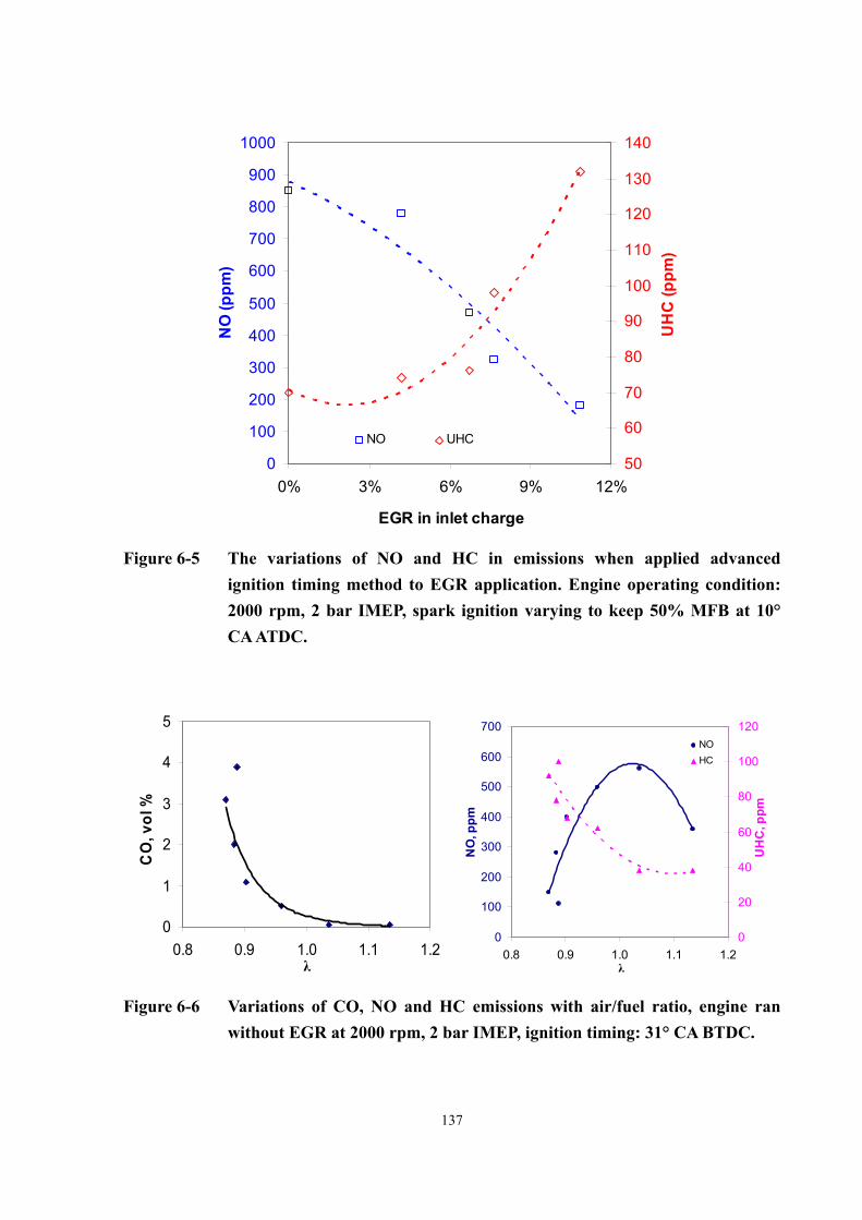
137

0

100

200

300

400

500

600

700

800

900

1000

0% 3% 6% 9% 12%

EGR in inlet charge

NO

(ppm

)

50

60

70

80

90

100

110

120

130

140

UH

C (p

pm)

NO UHC

Figure 6-5 The variations of NO and HC in emissions when applied advanced

ignition timing method to EGR application. Engine operating condition: 2000 rpm, 2 bar IMEP, spark ignition varying to keep 50% MFB at 10° CA ATDC.

0

1

2

3

4

5

0.8 0.9 1.0 1.1 1.2λ

CO

, vol

%

0

100

200

300

400

500

600

700

0.8 0.9 1.0 1.1 1.2λ

NO

, ppm

0

20

40

60

80

100

120

UH

C, p

pmNOHC

Figure 6-6 Variations of CO, NO and HC emissions with air/fuel ratio, engine ran

without EGR at 2000 rpm, 2 bar IMEP, ignition timing: 31° CA BTDC.

138

6.3. Adding H2 as an Additive in NG Fuel

Adding hydrogen to an engine as an additive has been found to produce a general trend of

enhancing the rate of combustion; as for emissions, UHC is observed reducing but NO

becomes higher when adding hydrogen. The characteristic stable combustion due to its fast

combustion rate can also make it efficient for extending the limit EGR that can be used.

Figure 6-7 presents the trends of combustion durations when adding H2 while varying the

ignition timing to retain 50% MFB at 10° CA ATDC, the reductions in combustion duration

can be observed in all stages of MFB. Figure 6-8 shows the trends of emissions from the test

in Figure 6-7, both of them shown the same tendencies as when adding hydrogen alone.

The combustion stabilizing effect of hydrogen can not be clearly recognized from the values

of COVIMEP, it fluctuated around the same level (1.4% in this case); however, the expected

increasing COVIMEP did not happen as shown in Figure 5-3 (A) when the ignition was

advanced from MBT timing, which shows the potential of using this strategy without causing

drivability problems. Through the comparisons between the cases with and without hydrogen

in Figure 6-9, a higher peak pressure and a steeper pressure rise can be clearly seen when

adding hydrogen (2.6% in volume this case). In the case of adding 4.8% EGR, the higher

pressure (in terms of crank angle) in the expansion stroke is further evidence of longer

combustion duration, which is correspondent to Figure 6-3 (A).

139

0

20

40

60

80

100

0% 1% 2% 3%H2 in inlet charge (vol.%)

Cra

nk a

ngle

(deg

.)

EOC 95% MFB 50% MFB 5% MFB

Figure 6-7 The variation of required crank angles in each MFB stage with increasing hydrogen, engine ran at 2000 rpm, 2 bar IMEP, ignition timing varying to keep 50% MFB at 10° CA ATDC.

650

750

850

950

0% 1% 2% 3%H2 in inlet charge (vol.%)

NO

, ppm

0

50

100

150

200

UH

C, p

pm

NO UHC

Figure 6-8 Variations of NO and HC emissions with hydrogen in the inlet charge, engine ran at 2000 rpm, 2 bar IMEP, ignition timing varying to keep maximum thermal efficiency.

140

0

4

8

12

16

0 150 300 450Volume (cm3)

Pres

sure

(bar

)

NG+2.6% H2NGNG+4.8% EGR

Figure 6-9 The variations of pressure versus volume when adding hydrogen or EGR

into the NG fuel, engine ran in the standard condition.

6.4. Combined effects of EGR & H2 – Fuel Reforming Simulation

6.4.1. Adding EGR and H2 Alternately – Investigation of the Trade-off Effect

Individual effects of EGR and hydrogen as additives in a NG fuelled engine have already

been discussed, one of the interesting topics in the present study is the combustion behaviour

when catalyst reformed gas is supplied to the engine, which means both EGR and hydrogen

are introduced into combustion and a trade-off effect will happen. Under such situation, the

combustion behaviour becomes complicated and hard to explain because there are too many

141

parameters; therefore, the comparisons will be based on some basic variations and with fewer

changes involved.

The approach of adding hydrogen to extend the EGR tolerance of a NG fuelled engine were

achieved through a ‘step increase’ method with 5% COVIMEP used as a criterion. The test

procedure starts once the base line condition has been reached, EGR is then added until the

criterion is slightly over, followed by applying hydrogen to bring the cycle by cycle variation

back to below 5%, meanwhile the ignition timing may be varied as required; by continuing to

do this, the limit of EGR can be gradually elevate until stable combustion can no longer be

retained by increasing hydrogen and/or varying the ignition timing.

6.4.1.1. Test 1.1 - Fixed Ignition Timing Test

5% and 50% MFB results in Figure 6-10 (A) show slightly decreasing trends, which are good

signs for the maximum thermal efficiency control. However, 95% MFB and EOC both reveal

a tendency to increase. At the beginning of combustion, hydrogen has a stronger effect on the

flame development period, which is why a shorter ignition delay was observed. However,

EGR delayed the burn duration - becoming severe even though the cycle by cycle variation

was controlled by the hydrogen, which implied the combustion rate should still remain within

a certain degree of its original speed, see the overlap of expansion stroke in Figure 6-10 (B).

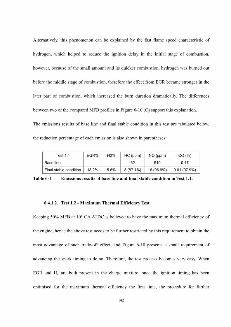
142

Alternatively, this phenomenon can be explained by the fast flame speed characteristic of

hydrogen, which helped to reduce the ignition delay in the initial stage of combustion,

however, because of the small amount and its quicker combustion, hydrogen was burned out

before the middle stage of combustion, therefore the effect from EGR became stronger in the

later part of combustion, which increased the burn duration dramatically. The differences

between two of the compared MFB profiles in Figure 6-10 (C) support this explanation.

The emissions results of base line and final stable condition in this test are tabulated below,

the reduction percentage of each emission is also shown in parentheses:

Test 1.1 EGR% H2% HC (ppm) NO (ppm) CO (%)

Base line - - 62 510 0.47

Final stable condition 18.2% 5.6% 8 (87.1%) 16 (96.9%) 0.01 (97.9%)

Table 6-1 Emissions results of base line and final stable condition in Test 1.1.

6.4.1.2. Test 1.2 - Maximum Thermal Efficiency Test

Keeping 50% MFB at 10° CA ATDC is believed to have the maximum thermal efficiency of

the engine, hence the above test needs to be further restricted by this requirement to obtain the

most advantage of such trade-off effect, and Figure 6-10 presents a small requirement of

advancing the spark timing to do so. Therefore, the test process becomes very easy. When

EGR and H2 are both present in the charge mixture, once the ignition timing has been

optimised for the maximum thermal efficiency the first time, the procedure for further

143

increasing the additives will become the same as test 1.1. Figure 6-11 illustrates such

condition; after the first time hydrogen was added to stabilize the combustion at spark timing

49° CA BTDC (5.67% EGR and 0.52% H2), the trend spark timing becomes level in the

continuative tests.

The emissions results of the base line and final stable conditions in this test are tabulated

below, the reduction percentage of each emission is also shown in parentheses:

Test 1.2 EGR% H2% HC (ppm) NO (ppm) CO (%)

Base line - - 90 710 0.51

Final stable condition 13.0% 1.7% 48 (46.7%) 126 (82.3%) 0.08 (84.3%)

Table 6-2 Emissions results of base line and final stable condition in Test 1.2.

6.4.2. Test 2 - Reformed Fuel Test

A synthetic gas with a volume composition of 75% H2 and 25% CO was used, aiming to

simulate the main reactive components of the product from the reforming reactor.

Comparisons between this gas and pure hydrogen were concentrated on the beneficial effects

in terms of combustion, i.e. whether the gas can maintain the stable combustion characteristic

and the low emissions level which are the greatest concerns in this study.

The trends of required crank angle degrees versus EGR in Figure 6-12 show very similar

behaviours at each MFB stages as in Figure 6-10. Results show that without sacrificing the

144

driving stability, 22.5% EGR in the inlet charge can be reached if the natural gas has 12.9%

enriched hydrogen. This outcome confirms the application of the exhaust gas reforming

method in terms of stable combustion.

The emissions results of the baseline and final stable conditions in this test are tabulated as

below, the reduction percentage in each emission is also shown in parentheses:

Test 2 EGR% H2% HC (ppm) NO (ppm) CO (%)

Base line - - 60 520 0.22

Final stable condition 22.5% 12.9% 48 (20%) 54 (89.6%) 0.1 (54.5%)

Table 6-3 Emissions results of base line and final stable condition in Test 2.

6.4.3. Peak Pressure

Figure 6-13 shows the correlation between peak pressure and the required crank angle degrees

in the above three tests, 5% MFB, 95% MFB and EOC are compared. Although the three

dotted trend lines all show similar declined tendencies, 5% MFB is more consistent, which

can be linked with the burn rate, thus more combustion will be conducted before TDC and

this causes higher pressure inside the cylinder, Figure 6-10 (B) and (C) shows these

phenomena.

The other signifier which should be addressed here is the consistency between the tendencies

of 95% MFB and EOC, this again confirms the EOC point has been acquired correctly.

145

6.4.4. Emissions Control

Figure 6-14 compares three emissions results from the above tests. They all show falling

tendencies with the increasing level of EGR, which supports the use of exhaust gas fuel

reforming and ensures its ability of exhaust control.

The synthetic gas did not perform better in terms of controlling CO and UHC; flatter curves

can be seen in related diagrams compared with the effect of adding pure hydrogen. The result

showing lean condition by adding EGR in test 1.2 has small effect on reducing CO, and this

can be ascribed to the CO content of synthetic gas.

A comparison of emissions control of the three tests is shown in Table 6-4. With similar EGR

content in the inlet charge, the synthetic gas performed very well, especially in NO control.

EGR% H2 % HC NO CO

Test 1.1 12.2% 4.9% 38.7% 65.7% 91.5%

Test 1.2 13.0% 1.7% 46.7% 82.3% 84.3%

Test 2 13.8% 5.9% 20.0% 75.8% 63.6%

Table 6-4 Percentage reductions of three emissions. Results shown are the comparisons between the baseline and the stable condition with similar EGR content in each test.

The strategy of increasing the tolerance of EGR using hydrogen enriched natural gas can be

achieved by interpolating the step procedure in Figure 6-10 ~ Figure 6-12, detailed method

can be found in the aforementioned IMechE paper by Allenby.

146

(A)

0

20

40

60

80

100

120

0% 5% 10% 15% 20%EGR in inlet charge (Vol.%)

Cra

nk a

ngle

(deg

.)

0%

1%

2%

3%

4%

5%

6%

H2 (

Vol.%

)

5% MFB 50% MFB 95% MFB EOC H2

(B)

0

2

4

6

8

10

12

14

16

0 150 300 450Cylinder volume (cm3)

Pres

sure

(bar

)

Base line18.2% EGR + 5.6% H2

(C)

360-10%

10%

30%

50%

70%

90%

110%

325 375 425Crank angle (degree)

MFB

base line

18.2%EGR+5.6% H2

Figure 6-10 (A) Required crank angle degrees versus EGR. Comparison of different MFB stages. Real line shows the test procedures in which EGR and H2 were added alternately. (B) P-V diagram and (C) MFB profile are comparisons between base line and test final condition. Engine ran in the standard condition with COVIMEP fluctuating about 5% (Test 1.1).

147

-60

-40

-20

0

20

40

60

0% 5% 10% 15%EGR in inlet charge (Vol.%)

Cra

nk a

ngle

ATD

C (d

eg.)

0.0%

0.5%

1.0%

1.5%

2.0%

H2 (

Vol.%

)

IG timing 5% MFB 50% MFB 95% MFB EOC H2

Figure 6-11 Required crank angle degrees versus EGR. Comparison of different MFB stages. Real line shows the test procedures in which EGR and H2 were added alternately. Engine ran in the standard condition with COVIMEP fluctuating about 5%, ignition timing was adjusted to keep 50% MFB at 10° CA ATDC (Test 1.2).

148

0.0% 0.0%

2.4%2.4%

4.7%4.6%

7.8% 7.6%

10.9%10.4%

13.9%13.7%

17.2%

0

20

40

60

80

100

120

0% 5% 10% 15% 20% 25%EGR in inlet charge (Vol.%)

Cra

nk a

ngle

(deg

.)

0%

2%

4%

6%

8%

10%

12%

14%

H2 (

Vol.%

)

5% MFB 50% MFB 95% MFB EOC H2

Figure 6-12 Required crank angle degrees versus EGR. Comparison of different MFB stages. Real line with H2/CO volume percentages shows the test procedure in which EGR and H2/CO were added alternately. Engine ran in the standard condition with COVIMEP fluctuating about 5%. (Test 1.3).

149

0

20

40

60

80

100

120

10.5 11 11.5 12 12.5 13 13.5PMax (bar)

Cra

nk a

ngle

(deg

.)

Test 1.1_EOC Test 1.2_EOC Test 2_EOCTest 1.1_95% Test 1.2_95% Test 2_95%Test 1.1_5% Test 1.2_5% Test 2_5%

5% MFB

95% MFB

EOC

Figure 6-13 Required crank angle degrees versus peak pressure. Comparison of 5%,

95% and total mass fraction burned.

150

0

0.1

0.2

0.3

0.4

0.5

0.6

0% 10% 20% 30%EGR (Vol.%)

CO

(%)

Test 1.1Test 1.2Test 2

0102030405060708090

100

0% 10% 20% 30%EGR (Vol.%)

UH

C (p

pm)

Test 1.1Test 1.2Test 2

0100200300400500600700800

0% 10% 20% 30%EGR (Vol.%)

NO

(ppm

)

Test 1.1Test 1.2Test 2

Figure 6-14 EGR versus emissions. Comparison of three combined effects tests.

151

7. APPLICATIONS OF DIFFERENTIAL PRESSURE DATA

Through the third differential of pressure data it is possible to detect the engine knocking, as

mentioned in the literature survey, which sheds lights on using the derivative of pressure data

to correlate with some other combustion phenomena. Differential pressure data are used to

locate the initial value of EOC in the improved method of MFB calculation, hence the first

and second derivatives of pressure traces are both available to provide for any further

applications. Work in this chapter will concentrate on two issues: MFB and emissions, using

the existing differential data to investigate the correlations.

Analysed pressure data were filtered by the nine points weighted smoothing method, the

differential values were derived by the following equation suggested by Checkel and Dale [8].

( )( ) ( ) ( ) ( )

( ) ( ) ( ) ( )( )

86 4 4 142 3 31188

193 2 2 126 1 1

P P P PdP d

P P P P

θ θ θ θθ θ

θ θ θ θ

× − − + + × + − + = × + × + − − + × + − −

Eq. 7-1

where

dP(θ) is the derivative value at crank angle θ.

dθ is the pressure data interval, one crank angle degree in this study.

P(θ) is the original pressure data at crank angle θ, (θ + 1) indicates the

succeeding crank angle and the same application applied for other items

in the equation.

152

7.1. Prediction of MFB

7.1.1. By Derivative Value

The second derivatives of cylinder pressure can be used to locate the ignition delay of a diesel

engine, 2% MFB, it has been said that it corresponds to d2p/dθ2 = 0 [94], although this value

is not adopted as the definition of ignition delay in this study, this relationship can be useful as

a validation method of MFB calculation.

Owing to the different working principles, the differential pressure patterns of spark ignition

engine are very different from those of a diesel engine, see Figure 7-1, and the pressure data

derived real time by data acquisition are not analogous, this will make the differential value

analysis more complex and unpredictable. Thus, after comparing with the three operating

conditions in Chapter 5, only the point (d2p/dθ2 = 0) in the standard operating condition

corresponds to 2% MFB as shown in Figure 7-1 (D). For the other two tests, they show little

relevant link at all, see Figure 7-2.

The method used in the program to estimate the initial EOC point for MFB calculation also

adopts a differential pressure tracking mechanism, which is also suggested by an application

to diesel engine [35]. Two options can be chosen in this method:

1. 1st derivative value: EOC locate at the minimum value position.

153

2. 2nd derivative value: EOC is the first zero point after the minimum value.

The same results from the above three operating conditions can be used again for comparing

the difference between these two methods. The comparative results are shown below:

Standard Lower speed Higher load 1st derivative value 396° CA 385° CA 384° CA 2nd derivative value 396° CA 385° CA 384° CA Final EOC point derived by improved method

419° CA 431° CA 432° CA

Table 7-1 Estimated EOC point by 1st and 2nd derivative value methods.

Both methods agree with each other, and all points happened earlier than the final EOC

positions, which means this method underestimates the EOC of a natural gas fuelled SI engine,

on the other hand, this proves that it is adequate as a starting point for the ‘approaching’

method, and both methods can be used without causing any difference in the end result.

For a mathematical aspect, these two options should reach the same result as shown in the

table; however, considering the discrete data condition, the second derivative value is highly

recommended for diesel engines.

7.1.2. By Integral of 2nd Derivative Values

This section investigates the potential method of predicting the required crank angles in each

MFB stage. The integration period was chosen from spark timing to the peak value of first

154

differential pressure, this period is the most rapid combustion period which affects the

cylinder pressure pronouncedly. However, the results have also been compared with the

integral values calculated throughout the whole combustion period, trends with different

directions but similar relationships were acquired. Trapezoidal rule is adopted to integrate the

data due to its simplicity.

The three tests conducted in Chapter 6 are compared to investigate the accuracy of the

prediction. Results in Figure 7-3 show pronounced consistency in each test; the linear

relationship can be applied through nearly all MFB stages in three tests, except the EOC with

higher variability. 5% and 50% MFB show very good correlations with the integral of 2nd

derivative, these phenomena can be contributed to the integration period which is roughly the

same as 50% MFB and the interval probably determines the whole pressure shape in the

diagram.

The linear relationship can be represented by the form as an equation y = Ax + B, the relative

parameters for each trend line are listed below:

5% MFB 50% MFB 95% MFB EOC

Test 1.1 y = -202.58x + 37.93 y = -305.45x + 68.54 y = -458.17x + 106.97 -

Test 1.2 y = -23.3x + 42.38 y = -20.43x + 64.3 y = -85.62x + 101.86 -

Test 2 y = -40.96x + 28.83 y = -69.18x + 53.61 y = -119.88x + 84.77 y = -172.23x + 116.07

Table 7-2 The linear equations of trend lines. Each equation represents the correlations between the integral of 2nd derivative of pressure data and required crank angles at relative MFB stage.

155

By mathematics, the integral of second derivative value should be equal to the subtraction of

the last and first value in the same period. Previous section also showing the EOC point

derived from the 1st derivative method or 2nd derivative method does not cause differences.

The results of comparison on the deviation between the values derived by the integration of

the 2nd derivative of pressure data during the ignition timing and peak pressure position, and

the subtraction value of the 1st derivative of pressure data between the ignition timing and

peak pressure, showing consistence in three compared cases, see Figure 7-4. The result

recommends the method of using the integration of 2nd derivative value is unnecessary; the

subtraction by the 1st derivative data can also perform the same function, which will make this

method more efficient.

156

(A)

0

2

4

6

8

10

12

14

170 220 270 320 370 420 470 520Crank angle (deg.)

Pres

sure

(bar

)

PressureIgnitionEOC

(B)

-0.3

-0.2

-0.1

0

0.1

0.2

0.3

170 220 270 320 370 420 470 520

Crank angle (deg.)

1st d

eriv

ativ

e of

pre

ssur

e da

ta

1st derivativeIgnitionEOC

(C)

-0.03

-0.025

-0.02

-0.015

-0.01

-0.005

0

0.005

0.01

170 220 270 320 370 420 470 520Crank angle (deg.)

2nd

deriv

ativ

e of

pre

sure

dat

a

2nd derivativeIgnitionEOC

(D)

360-0.03

-0.02

-0.01

0.00

0.01

325 345 365 385 405Crank angle (deg.)

2nd

deriv

ativ

e of

pre

sure

dat

a

2nd derivative Ignition EOC 2% MFB Figure 7-1 Pressure data patterns of natural gas fuelled engine. (A) Original pressure

data (B) 1st derivative of pressure data (C) 2nd derivative of pressure data (D) Relevant window of 2nd derivative of pressure data. Data shown are from a baseline test of the standard operating condition.

(A)

360-0.10

-0.08

-0.06

-0.04

-0.02

0.00

0.02

0.04

325 375 425Crank angle (deg.)

2nd

deriv

ativ

e of

pre

sure

dat

a

2nd derivative Ignition EOC 2% MFB

(B)

360-0.20

-0.15

-0.10

-0.05

0.00

0.05

0.10

325 375 425Crank angle (deg.)

2nd

deriv

ativ

e of

pre

sure

dat

a

2nd derivative Ignition EOC 2% MFB Figure 7-2 2% MFB position on the second differential pressure curve. Comparison

of (A) lower speed and (B) higher load conditions.

157

(A) Test 1.1

0

20

40

60

80

100

120

0.03 0.08 0.13 0.18Integral of 2nd derivative value

Cran

k an

gle

(deg

.)

5% MFB 50% MFB 95% MFB EOC

(B) Test 1.2

0

20

40

60

80

100

0.205 0.215 0.225 0.235Integral of 2nd derivative value

Cran

k an

gle

(deg

.)

5% MFB 50% MFB 95% MFB

(C) Test 2

0

20

40

60

80

100

0.045 0.055 0.065Integral of 2nd derivative value

Cran

k an

gle

(deg

.)

5% MFB 50% MFB 95% MFB

Figure 7-3 Correlation between MFB and integral of 2nd derivative of pressure data.

0

0.05

0.1

0.15

0.2

0.25

0 0.05 0.1 0.15 0.2 0.25Integral value of 2nd derivative

Subt

ract

ion

valu

e of

1st

der

ivar

ive Test 1.1

Test 1.2Test 2

Figure 7-4 The deviation between the integral value of 2nd derivative of pressure data

and the subtraction value of 1st derivative of pressure data.

158

7.2. Emissions pattern prediction

Natural gas fuelled engines normally produce lower emissions such as CO, UHC and

particulate than the traditional hydrocarbon fuels. Due to this clean characteristic, it stands a

better chance of the emissions being predictable by simply extracting information from the

combustion related data, e.g. differential pressure traces.

May [10] successfully correlated the integral of the second differential pressure data to predict

the emissions behaviour in a gasoline fuelled SI engine, this encourages a feasibility

investigation on applying such a mechanism to an SI engine with exhaust gas reformed fuel.

Although the above discussions has proved the 1st derivative can perform the same result, its

slight deviation might still cause some unexpected problems, therefore, the 2nd derivative

value is still adopted for comparing. The integral results from the last section are further

investigated for the correlation between the value and emissions results; however, in May’s

experiments, the comparisons were set up between different equivalence ratios and fuels,

which intended to minimize the change of the emission results. The attempt here is to try to

correlate the exhaust emissions from a more complicated mixture, which includes EGR and

H2 inside the natural gas fuel, although the stoichiometric condition was supposed to be

maintained, the inlet charge condition still fluctuated occasionally. Hence, IMEP and

maximum pressure are introduced to normalize the variability, these two values have direct

159

links with the air/fuel ratio; hence, dividing by one of them can normalize the variation.

7.2.1. Nitric Oxide

The formation of NO is linked to temperature and peak pressure as mentioned in Chapter 6;

hence, the integral value is divided by the peak pressure to normalize the variation. After

comparison, the whole combustion period was found not to improve the correlation, and the

best fit for this relationship is a linear behaviour, the results and the correlation equations are

shown in Figure 7-5. Correlation of Test 1.2 has higher variation mainly because the effect of

advanced ignition timing, which increased the peak pressure and will abate the effect of

normalization. This result is different with May’s, which an exponential function as Eq. 2-17

was reported, the reason is probably because the engine operation conditions were not stable

and the air/fuel ratio moved up and down between the stoichiometric, in May’s consideration,

they should be separated for comparison.

7.2.2. Carbon Monoxide

The deduction in the last section has already implied the impossibility of using this method to

predict the CO in these compared cases. Based on previous discussion, the air/fuel ratio

160

determines the amount of CO in the exhaust, however, the result with the same comparison

measure (by May’s method) is show in Figure 7-6. The expected logarithmic relationship can

not be clearly identified.

Although only NO can be correlated with the integral values in the present study, the

application is still optimistic, under more rigorous experimental set up, it is possible to foretell

the exhaust emissions behaviour simply from cylinder pressure data. The demonstration of

successful prediction of NO in this study is a good example.

0

50

100

150

200

250

300

-0.03 -0.02 -0.01 0 0.01 0.02 0.03Integral of 2nd derivative value/Pmax

NO

(ppm

)

Test 1.1

Test 1.2

Test 2

Test 1.1 y = -9281.7x + 2.561 Test 1.2 y = -39042x + 902.15 Test 2 y = -39238x + 279.4

Figure 7-5 Correlations of NO and the integral of 2nd derivative of pressure data divided by peak pressure

161

0

0.02

0.04

0.06

0.08

0.1

0.12

0 0.1 0.2 0.3Integral of 2nd derivative value

CO

(%)

Test 1.1Test 1.2Test 2

Figure 7-6 CO versus the integral of 2nd derivative of pressure data.

162

8. CONCLUSIONS AND FUTURE WORK

8.1. Conclusions

According to the test results and previous discussions, a number of conclusions can be drawn

and generally classified into three categories.

8.1.1. Accuracy of Improved Methods

The accuracy of the improved method has been verified for three operating conditions, the

deviation at each MFB stage between this method and other traditional measures, even with

the same combustion period, can be very high, e.g. 15% at 5% MFB, 9.76% at 50% MFB and

30.28% at 95% MFB. This also reveals the importance of choosing the data processing

method; the difference in MFB calculation result between the raw data and smoothed signals

has been found to deviate by 65% deviation in some cases.

A mechanism for finding the EOC position without objective judgement involved has been

established and associated with the MFB calculation, the results always shows a convergence

in the approaching process. The compression and expansion polytropic indices are both

derived from the pressure data by a curve fitting method to gain linear regressions with better

approximations, and then used together with the approached EOC point in the calculation of

163

the revised R&W model to derive the final MFB result.

8.1.2. The Correlations between Additives and Combustion Related Indicators

The effects of EGR and hydrogen on the natural gas fuelled SI engine have been investigated

in terms of combustion duration. These effects were quantified and then used successfully to

correlate the more complicated behaviour in the operating condition with reformed fuel.

The use of synthetic gas containing 75% H2 and 25% CO was verified as performing well in

terms of emissions control, while the burn duration can be maintained at nearly the same level

as for the condition when adding pure hydrogen is added. This phenomenon also confirms the

envelope of benefits of using exhaust gas fuel reforming in a NG fuelled SI engine.

8.1.3. Using Differential Pressure Data to Predict the MFB and Emissions

The first CA point after ignition with the value d2p/dθ2 = 0 has been found to correspond to

2% MFB in only some special cases, which is not suitable to be used in a natural gas fuelled

SI engine. Also, the first occurrence of the zero value seems to be quite random, in conclusion

this method is not very relevant to establishing the ignition delay. In contrast, tracking the first

and second derivative value to locate the EOC point has shown that it underestimates the

164

combustion duration, however, it can be used as an initial value in the EOC finding

mechanism.

The integral of the 2nd derivative of pressure data has proved itself a useful tool for predicting

the required crank angles at each MFB stage. However, the method using the subtraction of

two relative 1st derivatives can reach the consistent results has shown the possibility of using a

simpler method to perform the same prediction. To the author’s knowledge, other researchers

have not previously used both methods.

The model of predicting the emission behaviour has shown some interesting results, NO level

can be foretold using the normalized integral value of the 2nd derivative of pressure data in a

linear equation form.

8.2. Future Work

8.2.1. Data Acquisition Rig

The data acquisition rig has at times suffered from the missing signals and system

malfunction problems during the tests. A signal conditioner, which was not used in this study,

should be used before signals pass to the data acquisition card. For reducing noise and any

interference, a better shielding material for cable and connections is also necessary. Instead of

165

smoothing data through program, a hardware filter might be added for dada accuracy.

8.2.2. Program

There are still too many parameters that have to be manually input to the program, and some

values have to be acquired from other sources, such as pressure gauge and flow meter, which

will reduce the accuracy. A self calibrating function can be employed to the in-house program

without too much effort, e.g. engine speed and absolute pressure pegging, which both affect

the MFB calculation. The former work can be done by just programming, but the latter will

need one more pressure transducer to be installed on the inlet manifold pipe. This way human

error can be avoided and tests will become more efficient.

To make it easy to obtain the data for comparison, the current program has not been

automated with the improved approaches with r-R&W model, the switching procedure needs

to be done manually. Besides, the MFB calculation has repeated the EOC finding mechanism

and polytropic index acquiring procedures in the program, which might cause delay for real

time study, therefore the program needs to be reprogrammed for better efficiency.

166

8.2.3. MFB Model

The r-R&W model is derived from the original R&W model. Although the use of two

polytropic index values in the revised model has already adopted the idea of two different

thermodynamics processes, which means some heat loss has occurred, the final result still

shows 100% of energy conversion. This can not be true in the real world, therefore a heat

transfer model has to be employed if the surface area of engine is known precisely.

The EOC position could be verified by an observation in an optical engine to confirm the

accuracy; an overestimated duration is expected without a heat transfer model.

The linear change of polytropic index method for MFB calculation has shown some

consistence with the improved method, which might be worth further studying in terms of its

thermodynamics aspect.

8.2.4. Emissions prediction

The method needs to be applied under more rigorous set up such as control of air/fuel ratio

condition, it is necessary to build up some baseline data before moving on to the reformed

fuel investigation, e.g. fuelling tests for different air/fuel ratio conditions with natural gas

alone, individual effect of additive on emissions in different air/fuel ratios, etc. The 1st

167

derivative and 2nd derivative of pressure data should both be examined the possibility of

prediction.

168

REFERENCES

1. Stone, R., et al., Combustion analysis in the Rover K4 optical engine. Proceeding of Institution of Mechanical Engineers C524/033/97, 1997. v. AutoTech '97(Automotive Engines and Powertrains): pp. 1-12.

2. Reeves, M., et al., Particle image velocimetry analysis of IC engine in-cylinder flows. Optics and Lasers in Engineering, 1996. v. 25(6): pp. 415-432.

3. Amann, C.A., Cylinder-pressure measurement and its use in engine research. SAE 852067, 1985.

4. Wibberley, P. and Clark, C.A., An investigation of cylinder pressure as feedback for control of internal combustion engines. SAE 890396, 1989.

5. Hayes, I.K., Savage, L.D., and Sorenson, S.C., Cylinder pressure data acquisition and heat release analysis on a personal computer. SAE 860029, 1986.

6. Chun, K.M. and Heywood, J.B., Estimating heat-release and mass-of-mixture burned from spark-ignition engine pressure data. Combustion Science and Technology, 1987. v. 54: pp. 133-143.

7. Stone, C.R. and Green-Armystage, D.I., Comparision of methods for the calculation of mass fraction burnt from engine pressure-time diagrams. Proceeding of Institution of Mechanical Engineers, 1987. v. 1201(D1): pp. 61-67.

8. Checkel, M.D. and Dale, J.D., Computerized knock detection from engine pressure recoeds. SAE 860028, 1986. v. 95: pp. 221-231.

9. Rosseel, E. and Sierens, R., Knock detection in a hydrogen engine. SAE 970039, 1997: pp. 37-47.

10. May, J.M. and Gyorog, D., A second derivation of cylinder pressure characterization of exhaust emissions. ASME, 1997 Spring Techanical Conference 97-ICE-30, 1997. v. 28-3: pp. 55~60.

11. Heywood, J.B., Internal combustion engine fundamentals. Automotive Technology. 1988: McGraw-Hill Book Company, ISBN 0-07-100499-8.

169

12. Ramos, J.I., Internal combustion engine modeling. 1989: Hemisphere Publishing Corporation, ISBN 0-89116-157-0. pp. 236-239.

13. Chow, A. and Wyszynski, M.L., Thermodynamic modelling of complete engine systems - a review. Proceeding of Institution of Mechanical Engineers, Part D: Journal of Automobile Engineering D03198, 1999. v. 213.

14. Rassweiler, G.M. and Withrow, L., Motion pictures of engine flames correlated with pressure cards. SAE, 1938. v. 42(5): pp. 185-204.

15. Larminie, J. and Dicks, A., Fuel cell systems explained. 2000: John Wiley & Sons, LTD, ISBN 0-471-49026-1.

16. Kordesch, K. and Simader, G., Fuel cells and their applications. 1996: VCH, ISBN 3-527-28679-2.

17. Blarigan, P.V. and Keller, J.O., A hydrogen fuelled Internal combustion engine designed for single speed/power operation. Internation Jurnal of Hydrogen Energy, 1998. v. 23(7): pp. 603-609.

18. Yamin, J.A.A., et al., Effect of combustion duration on the performance and emission characteristics of a spark ignition engine using hydrogen as a fuel. International Journal of Hydrogen Energy, 2000. v. 25: pp. 581-589.

19. Borroni-Bird, C.E., Fuel cell commercialization issues for light-duty vehicle applications. Journal of Power Sources, 1996. v. 61: pp. 33-48.

20. Ekdunge, P. and Raberg, M., The fuel cell vehicle analysis of energy use, emissions and cost. International Journal of Hydrogen Energy, 1998. v. 23: pp. 381-385.

21. Meyer, A.P., et al., Progress in the development of PEM fuel cell engines for transportation. SAE 2001-01-0540, 2000.

22. Taraza, D., Henein, N.A., and Bryzik, W., The frequency analysis of the crankshaft's speed variation: A reliable tool for diesel engine diagnosis. Journal of Engineering for Gas Turbines and Power, 2001. v. 123(2): pp. 428-432.

23. Chan, S.H., Thermodynamics in a turbocharged direct injection diesel engine. Proceedings of the Institution of Mechanical Engineers, Part D: Journal of Automobile Engineering, 1998. v. 212(1): pp. 11-24.

170

24. Saitzkoff, A., et al., In-cylinder pressure measurements using the spark plug as an ionization sensor. SAE 970875, 1997. v. 106.

25. Brown, W.L., Methods for evaluating requirements and errors in cylinder pressure measurement. SAE 670008, 1967. v. 76: pp. 50-77.

26. Lancaster, D.R., Krieger, R.B., and Lienesch, J.H., Measurement and analysis of engine pressure data. SAE 750026, 1975

27. Randolph, A.L., Cylinder-pressure-transducer mounting techniques to maximize data accuracy. SAE 900171, 1990. v. 99.

28. Collings, N., Dinsdale, S., and Eade, D., Knock detection by means of the spark plug. SAE 860635, 1986.

29. Ohashi, Y., et al., The application of ionic current detection system for the combustion condition control. SAE 1999-01-0550, 1999. v. SP-1419.

30. VanDyne, E.A., et al., Misfire detection from ionization feedback utilizing the SmartFire plasma ignition technology. SAE 2000-01-1377, 2000.

31. Byttner, S., Rognvaldsson, T., and Wickstrom, N., Estimation of combustion variability using in-cylinder ionization measurements. SAE 2001-01-3485, 2001.

32. Daniels, C.F., The comparison of mass fraction burned obtained from the cylinder pressure signal and spark plug ion signal. SAE 980140, 1998. v. SP-1348: pp. 15-23.

33. Daw, C.S. and Kahl, W.K., Interpretation of engine cycle-to-cycle variation by chaotic time series analysis. SAE 902103, 1990. v. 99: pp. 2188-2199.

34. Guezennec, Y.G. and Gyan, P., A novel approach to real-time estimation of the individual cylinder combustion pressure for S.I. engine control. SAE 1999-01-0209, 1999: pp. 55-65.

35. Reddy, P.R., et al., Evaluation of combustion parameters in direct injection diesel engines - An easy and reliable method. SAE 930605, 1993. v. SP-971: pp. 159~165.

36. Gatowski, J.A., et al., Heat release analysis of engine pressure data. SAE 841359, 1984: pp. 961-977.

171

37. Cheung, H.M. and Heywood, J.B., Evaluation of a one zone burn-rate analysis procedure using production SI engine pressure data. SAE 932749, 1993. v. 102: pp. 2292-2303.

38. Cartwright, A. and Fleck, R., Cylinder pressure analysis in high performance two-stroke engines. SAE 962535, 1996. v. 105.

39. Jensen, T.K. and Schramm, J., A three-zone heat release model for combustion analysis in a natural gas SI engine - effects of crevices and cyclic variations on UHC emissions. SAE 2000-01-2802, 2000.

40. Hassaneen, A.E., et al., A study of the flame development and rapid burn durations in a lean-burn, fuel-injected natural gas S.I. engine. SAE 981384, 1998. v. SP-1371.

41. Brunt, M.F.J. and Emtage, A.L., Evaluation of IMEP routines and analysis errors. SAE 960609, 1996: pp. 87-101.

42. Rocco, V., D.I. diesel engine in-cylinder pressure data analysis under T.D.C. setting error. SAE 930595, 1993.

43. Stas, M.J., Thermodynamic determination of T.D.C. in piston combustion engines. SAE 960610, 1996. v. SP-1157: pp. 103-108.

44. Morishita, M. and Kushiyama, T., An improved method for determining the TDC position in a PV-diagram (First report). SAE 970062, 1997. v. 106: pp. 233-244.

45. Morishita, M. and Kushiyama, T., An improved method of determining the TDC position in a PV-diagram. SAE 980625, 1998. v. SP-1330.

46. Tazerout, M., Corre, O.L., and Rousseau, S., TDC determination in IC engines based on the thermodynamic analysis of the temperature-entropy diagram. SAE 1999-01-1489, 1999. v. 108.

47. Brunt, M.F.J. and Emtage, A.L., Evaluation of burn rate routines and analysis errors. SAE 970037, 1997: pp. 19-30.

48. Brunt, M.F.J. and Pond, C.R., Evaluation of techniques for absolute cylinder pressure correction. SAE 970036, 1997. v. SP-1267: pp. 7-18.

49. Randolph, A.L., Methods of processing cylinder-pressure transducer signals to maximize data accuracy. SAE 900170, 1990. v. 99.

172

50. Brunt, M.F.J. and Lucas, G.G., The effect of crank angle resolution on cylinder pressure analysis. SAE 910041, 1991.

51. Karim, G.A. and Khan, M.O., An examination of some of the error normally associated with the calculation of apparent rates of combustion heat release in engines. SAE 710135, 1971.

52. Shayler, P.J., Wiseman, M.W., and Ma, T., Improving the determination of mass fraction burnt. SAE 900351, 1990.

53. Ball, J.K., Raine, R.R., and Stone, C.R., Combustion analysis and cycle-by-cycle variations in spark ignition engine combustion Part 1: An evaluation of combustion analysis routines by reference to model data. Proceedings of the Institution of Mechanical Engineers, Part D: Journal of Automobile Engineering D04197, 1998. v. 212: pp. 381-339.

54. Homsy, S.C. and Atreya, A., An experimental heat release rate analysis of a diesel engine operating under steady state conditions. SAE 970889, 1997. v. SP-1246.

55. Rauckis, M.J. and McLean, W.J., The effects of hydrogen addition on ignition delays and flame propagation in spark ignition engines. Combustion Science and Technology, 1998. v. 19: pp. 207-216.

56. Grimm, B.M. and Johnson, R.T., Review of simple heat release computations. SAE 900445, 1990.

57. Hribernik, A., Statistical determination of correlation between pressure and crankshaft angle during indication of combustion engines. SAE 982541, 1998.

58. Mendis, K.J.S., et al., Modelling and measurements from a natural gas fuelled engine. SAE 930927, 1993. v. SP-958: pp. 143-161.

59. Ferguson, C.R. and Kirkpatrick, A.T., Internal combustion engines applied thermosciences. 2nd ed. 2001: John Wiley & Sons, Inc, ISBN 0-471-35617-4.

60. Stone, C.R., Brown, A.G., and Beckwith, P., Cycle-by-cycle variations in spark ignition engine combustion - Part II: Modelling of flame kernel dispalccements as a cause of cycle-by-cycle variations. SAE 960613, 1996. v. SP-1157.

61. Ozdor, N., Dulger, M., and Sher, E., An experimental study of the cyclic variability in spark ignition engines. SAE 960611, 1996. v. SP-1157.

173

62. Johansson, B., Cycle-to-cycle variations in S.I. engines - the effects of fluid flow and gas composition in the vicinity of the spark plug on early combustion. SAE 962084, 1996. v. 105: pp. 2281-2296.

63. Brunt, M.F.J., Rai, H., and Emtage, A.L., The calculation of heat release energy from engine cylinder pressure data. SAE 981052, 1998. v. SP-1315: pp. 101-112.

64. Ishii, K., et al., Investigation of cyclic variation of IMEP under lean burn operation in spark-ignition engine. SAE 972830, 1997. v. SP-1301: pp. 55-64.

65. Austen, A.E.W. and Lyn, W.T., The application of heat release analysis to engine combustion study. CIMAC Conference, International Council on Combustion Engines, 1962.

66. Krieger, R.B. and Borman, G.L., The computation of apparent heat release for internal combustion engines. ASME 66-WA/DGP-4, 1966.

67. Goering, C.E., Engine heat release via spread sheet. American Society of Agricultural Engineers, 1998. v. 41(5): pp. 1249-1253.

68. Woschni, G., A universially applicable equation for the instantaneous heat transfer coefficient in the internal combustion engine. SAE 670931, 1967. v. 76.

69. Eichelberg, I.G., Some new investigations on old combustion engine problems - II. Engineering, 1939. v. 148: pp. 463-466, 547-550.

70. Annand, W.J.D., Heat transfer in the cylinders of reciprocating internal combustion engines. Proceeding of Institution of Mechanical Engineers, 1963. v. 177(36): pp. 973~990.

71. Annand, W.J.D. and Ma, T.H., Instantaneous heat transfer rates to the cylinder head surface of a small compression-ignition engine. Proceeding of Institution of Mechanical Engineers, 1971. v. 185(Part 1): pp. 976~987.

72. Whitehouse, N.D., Heat transfer in a quiescent chamber diesel engine. Proceeding of Institution of Mechanical Engineers, 1971. v. 185, Part 1: pp. 963-975.

73. Han, S.B., et al., Empirical formula for instantaneous heat transfer coefficient in spark ignition engine. SAE 972995, 1997. v. SP-1306.

174

74. Patro, T.N., Combustion study of hydrogen fueled DI diesel engine: Simplified heat release analysis. International Journal of Hydrogen Energy, 1993. v. 18(3): pp. 231-241.

75. Goodger, E.M., Alternative fuels - Chemical energy resources. 1980: The Macmillan Press Ltd, ISBN 0-333-25813-4.

76. Poulton, M.L., Alternative fuels for road vehicles. 1994: Computational Mechanics Publications, ISBN 1-85312-301-3.

77. Maxwell, T.T. and Jones, J.C., Alternative fuels: emissions, economics, and performance. 1995: Society of Automotive Engineers, ISBN 1560915234.

78. Kato, K., et al., Development of engine for natural gas vehicle. SAE 1999-01-0574, 1999. v. SP-1436

79. Swain, M.R., et al., The effects of hydrogen addition on natural gas engine operation. SAE 932775, 1993. v. 102: pp. 1592-1601.

80. Liss, W.E. and Thrasher, Natural gas as a stationary engine and vehicular fuel. SAE 912364, 1991. v. SP-888

81. Das, L.M. and Mathur, R., Exhaust gas recirculation for NOx control in a multicylinder hydrogen-supplemented S.I. engine. Internation Jurnal of Hydrogen Energy, 1993. v. 18(12): pp. 1013-1018.

82. Lumsden, G., Eddleston, D., and Sykes, R., Comparing lean burn and EGR. SAE 970505, 1997. v. SP-1267

83. Sakonji, T. and Shoji, F., Study on improvement of natural gas fueled spark ignition engines - effect of EGR utilization. SAE 971714, 1997.

84. Apostolescu, N. and Chiriac, R., A study of combustion of hydrogen-encriched gasoline in a spark Ignition engin. SAE 960603, 1996. v. SP-1157.

85. Stocky, J.F., Dowdy, M.W., and Vanderbrug, T.G., An examation of the performance of spark ignition engines using hydrogen-supplemented fuels. SAE 750027, 1975.

86. Shrestha, S.O.B. and Karim, G.A., Hydrogen as an additive to methane for spark ignition engine applications. International Journal of Hydrogen Energy, 1999. v. 24: pp. 577-586.

175

87. Jones, M.R., Dunn, J.W., and Wyszynski, M.L., Thermodynamics feasibility studies of the exhaust-gas reforming of hydrocarbon fuels. Proceeding of Institution of Mechanical Engineers, Part D, C384/014, 1990.

88. Jones, M.R. and Wyszynski, M.L., Onboard generation of hydrogen-based gaseous engine fuels by exhaust-gas reforming of liquid hydrocarbons. Auto Tech '93, 1993.

89. Jamal, Y. and Wyszynski, M.L., On-board generation of hydrogen-rich gaseous fuels-a review. International Journal of Hydrogen Energy, 1994. v. 19(7): pp. 557-572.

90. Wagner, T., Jamal, Y., and Wiszynski, M.L., Advantages of fractional addition of hydrogen to internal combustion engines by exhaust gas fuel reforming. Hypothesis Conference, Cassino-Gaete, Italy. 26-29 June, 1995.

91. Jamal, Y., Wagner, T., and Wyszynski, M.L., Exhaust gas reforming of gasoline at moderate temperatures. International Journal of Hydrogen Energy, 1996. v. 21(6): pp. 507-519.

92. Wyszynski, M.L., et al., On-board generation and IC engine use of hydrogen-rich gaseous fuels. Hydrogen 94,10th World Hydrogen Conference, 1994: pp. 1-10.

93. Smith, J.A. and Bartley, G.J.J., Stoichiometric operation of a gas engine utilizing synthesis gas and EGR for NOx control. ASME, 1998 Spring Techanical Conference 98-ICE-107, 1998. v. 30(3): pp. 59-66.

94. Sher, E. and Hacohen, Y., Ignition delay and combustion duration in H2-enriched gasoline SI engine. Combustion Science and Technology, 1989. v. 65: pp. 263-275.

95. Tabaczynski, R.J., Ferguson, C.R., and Radhakrishnan, K., A turbulent entrainment model for spark-ignition engine combustion. SAE 770647, 1977. v. 86.

96. Hires, S.D., Tabaczynski, R.J., and Novak, J.M., The prediction of ignition delay and combustion intervals for a homogeneous charge, spark ignition engine. SAE 780232, 1978. v. 78.

97. Blizard, N.C. and Keck, J.C., Experimental and theoretical investigation of turbulent burning model for internal combustion engines. SAE 740197, 1974. v. 83.

98. Stone, R., Introduction to internal combustion engines. 3rd ed. 1999: MacMillan Press Ltd., ISBN 0-333-74013-0.

176

99. Allenby, S., et al., Hydrogen enrichment: A way to maintain combustion stability in a natural gas fuelled engine with exhaust gas recirculation, the potential of fuel reforming. Proceeding of Institution of Mechanical Engineers, 2001. v. 215(Part D: Journal of Automobil Engineering): pp. 405~418.

100. Namazian, M. and Hwywood, J.B., Flow in the piston cylinder ring crevices of a spark ignition engine, effect on hydrocarbon emissions, efficiency and power. SAE 820088, 1982

101. Degobert, P., Automobiles and Pollution. 1995: SAE, ISBN 1-56091-563-3.

177

APPENDIX - A

Dead weight calibrations for pressure transducer and charge amplifier set.

Pressure(bar) 1 2 3 4 Average 0 -0.146 -0.179 -0.154 -0.177 -0.164 1 -0.089 -0.123 -0.097 -0.119 -0.107 1.5 -0.063 -0.093 -0.069 -0.091 -0.079 2 -0.038 -0.064 -0.042 -0.064 -0.052 2.5 -0.012 -0.037 -0.015 -0.038 -0.0255 3 0.012 -0.011 0.011 -0.01 0.0005 3.5 0.037 0.014 0.039 0.015 0.02625 4 0.064 0.04 0.066 0.042 0.053 4.5 0.089 0.067 0.092 0.068 0.079 5 0.115 0.094 0.117 0.094 0.105 5.5 0.142 0.12 0.144 0.119 0.13125 6 0.169 0.148 0.17 0.148 0.15875 6.5 0.197 0.174 0.195 0.175 0.18525 7 0.224 0.201 0.222 0.201 0.212 7.5 0.25 0.228 0.249 0.227 0.2385 8 0.276 0.253 0.277 0.254 0.265 8.5 0.301 0.279 0.304 0.281 0.29125 9 0.324 0.306 0.329 0.308 0.31675 9.5 0.351 0.334 0.355 0.335 0.34375 10 0.379 0.361 0.38 0.362 0.3705 10.5 0.405 0.387 0.408 0.388 0.397 11 0.431 0.416 0.434 0.415 0.424 11.5 0.458 0.444 0.46 0.442 0.451 12 0.484 0.471 0.486 0.468 0.47725 12.5 0.511 0.497 0.509 0.495 0.503 13 0.538 0.524 0.536 0.521 0.52975 13.5 0.565 0.55 0.563 0.547 0.55625 14 0.592 0.576 0.589 0.575 0.583 14.5 0.618 0.603 0.616 0.601 0.6095 15 0.645 0.63 0.644 0.627 0.6365 15.5 0.671 0.656 0.671 0.653 0.66275 16 0.698 0.681 0.7 0.681 0.69 16.5 0.724 0.708 0.727 0.708 0.71675 17 0.75 0.735 0.753 0.736 0.7435 17.5 0.777 0.761 0.777 0.762 0.76925 18 0.805 0.789 0.801 0.79 0.79625 18.5 0.83 0.814 0.829 0.816 0.82225 19 0.857 0.843 0.856 0.843 0.84975 19.5 0.883 0.87 0.883 0.87 0.8765 20 0.91 0.896 0.909 0.897 0.903 20.5 0.935 0.924 0.935 0.923 0.92925

178

Pressure(bar) 1 2 3 4 Average 21 0.965 0.949 0.962 0.949 0.95625 21.5 0.992 0.976 0.99 0.975 0.98325 22 1.014 1.003 1.013 1.002 1.008 22.5 1.043 1.03 1.04 1.029 1.0355 23 1.074 1.059 1.066 1.054 1.06325 23.5 1.093 1.083 1.094 1.079 1.08725 24 1.123 1.112 1.121 1.104 1.115 24.5 1.15 1.138 1.148 1.13 1.1415 25 1.174 1.166 1.172 1.155 1.16675 25.5 1.199 1.192 1.198 1.182 1.19275 26 1.225 1.216 1.223 1.213 1.21925 26.5 1.255 1.242 1.259 1.24 1.249 27 1.283 1.272 1.285 1.264 1.276 27.5 1.308 1.297 1.311 1.29 1.3015 28 1.332 1.326 1.335 1.32 1.32825 28.5 1.355 1.347 1.356 1.345 1.35075 29 1.385 1.375 1.384 1.375 1.37975 29.5 1.409 1.405 1.41 1.402 1.4065 30 1.438 1.429 1.436 1.432 1.43375 30.5 1.464 1.459 1.463 1.458 1.461 31 1.491 1.482 1.49 1.485 1.487 31.5 1.519 1.509 1.515 1.509 1.513 32 1.543 1.538 1.543 1.538 1.5405 32.5 1.565 1.562 1.569 1.566 1.5655 33 1.594 1.588 1.591 1.593 1.5915 33.5 1.616 1.611 1.615 1.616 1.6145 34 1.646 1.637 1.649 1.644 1.644 34.5 1.674 1.664 1.674 1.672 1.671 35 1.694 1.699 1.701 1.698 1.698 35.5 1.72 1.72 1.727 1.723 1.7225

179

APPENDIX - B

The deduction of IMEP calculation used in the program:

Substitute Eq. 4-4 into Eq. 4-3

( )2 2 2

2 21 cos sin4 2 4 4cB L B LV V l lπ πθ θ = + + − − −

Eq. B-1

( )2

2

22 2

sin 28sin

4 2sin

4

LdV B Ld Ll

θπ θθ

θ

= +

−

Eq. B-2

Substitute Eq. B-2 into Eq. 2-8

( )( )

0

2

2

22 2

sin 28sin

4 2sin

4

n

is

L iB LIMEP p i iV Ll i

θ

θ

θ π=

∆ = +

−

∑ Eq. B-3