ezzone an online tool for delineating management zones

EZZone – An Online Tool for Delineating Management Zones

Camden Lowrance1,2, Spyros Fountas3, Vasileios Liakos2, George Vellidis2

1Sharpe Technology Solutions, Tifton, GA, USA

2Crop and Soil Sciences Department, University of Georgia, Tifton, Georgia, USA

3Department of Resource Management and Agricultural Engineering, Agricultural University of Athens, Athens, Greece

A paper from the Proceedings of the

13th International Conference on Precision Agriculture

July 31 – August 4, 2016

St. Louis, Missouri, USA

Abstract. Management zones are a pillar of Precision Agriculture research. Spatial variability is apparent in all fields, and assessing this variability through measurement devices can lead to better management decisions. The use of Geographic Information Systems for agricultural management is common, especially with management zones. Although many algorithms have been produced in research settings, no online software for management zone delineation exists. This research used a common grouping technique based on minimizing the sum of squares between groups to create an open source tool called EZZone for management zone delineation. The tool is accessible by anyone at ezzone.pythonanywhere.com, and allows users to upload their data for delineation. The tool is designed to be user friendly and easily integrate with other GIS software. EZZone was applied and evaluated on data collected from small to large fields, as well as fields incorporating Variable Rate Technology. Five fields were chosen from Georgia, USA, the UK and Greece. The zones were constructed in these fields until the Goodness of Variance fit was above 0.8. The results for each field are discussed and the strengths and weaknesses of the algorithm are examined.

Keywords. Management Zones, Precision Agriculture, GIS, Web Applications, Free Software.

The authors are solely responsible for the content of this paper, which is not a refereed publication. Citation of this work should state that it is from the Proceedings of the 13th International Conference on Precision Agriculture. Lowrance, C., S. Fountas, and G. Vellidis. (2016). EZZone – An Online Tool for Delineating Management Zones . In Proceedings of the 13th International Conference on Precision Agriculture (unpaginated, online). Monticello, IL: International Society of Precision Agriculture.

Proceedings of the 13th International Conference on Precision Agriculture July 31 – August 3, 2016, St. Louis, Missouri, USA

Introduction

Precision Agriculture’s Importance, Drawbacks, and Application in this Research

Precision agriculture (PA) is a catch-all term for techniques, technologies, and management strategies aimed at addressing within-field variability of parameters that affect crop growth. The goal of using these smart technologies is to increase profitability by maximizing output (yield) while optimizing inputs (water, fertilizer, labor etc.) by treating the field as a continually varying surface and adapting unique management to these varying zones of the field (Cook & Bramley, 1998). The economic benefits of precision farming are well-documented and these techniques have the potential to lessen the environmental impacts of agriculture while increasing profitability (Katalin, Rahoveanu, Magdalena, & István, 2014). However, the ability of small-scale farmers to adopt these technologies is limited because of the high costs associated with the technology (Lamb, Frazier, & Adams, 2008) and also because the development of new technology is designed for large scale production (Cook & Bramley, 1998).

One major drawback of current technology is its usability by farmers (Robertson et al., 2012). Learning how to use new software or hardware is time consuming and often not seen as worthwhile for farmers. Farmers are less likely to invest time and money into technology that is overly complex. New technology should focus on providing farmers with valuable information at minimal time investment and maximal usability

Management Zone Use in Precision Agriculture

A management zone is a portion of a field that is more homogenous than the overall field based on a certain measureable characteristic (Zhang, Wang, & Wang, 2002). Management zones (MZs) in PA have been used to increase crop productivity, optimize inputs, and reduce environmental costs. MZs are particularly important when Variable Rate Technology (VRT) is used to vary the rate of agricultural inputs such as fertilizer, lime, or water (Fleming, Westfall, Wiens, & Brodahl, 2000). The zones can be integrated with application equipment to actively control the amount of an input dispersed. Variable Rate Irrigation (VRI) can incorporate defined management zones to determine irrigation amounts in VRI center pivot technology (Vellidis, Tucker, Perry, Kvien, & Bednarz, 2008). When integrated with real time field monitoring, MZs allow farmers to precisely control irrigation amounts throughout their fields.

It is important to choose proper characteristics to use in MZs classification. The majority of field characteristics used for determination are temporally stable and correlated with yield. Soil measurements such as electrical conductivity (EC) and fertility are common input parameters. Since soil EC variability also represents variability of other soil properties, it has become a common measure for zone definition (Li, Shi, & Li, 2007). The measurement is easy to obtain and is often correlated with crop yield.

The process of creating management zones can be daunting for anyone unfamiliar with spatial relationships and analysis. There exists currently one commonly used free tool for management zone delineation, a Windows based software known as Management Zone Analyst (Fridgen et al., 2004). This software has drawbacks that are directly addressed by this research project. The tool produced by this research is be user friendly and as automated as possible. It also easily incorporates with other GIS software by outputting the zones in common GIS file formats.

Management Zone Delineation Techniques

The basis of all management zone delineation (MZD) techniques is grouping of data values into similar classes so that the members of the class are closer in relation than to members of other classes (Lark, 1998). Although a variety of techniques have been used or proposed, there is no standard procedure and the success of a procedure is largely determined by the input dataset (Guastaferro et al., 2010).

Fuzzy c-means (or k-means) is a common technique for clustering data. The technique seeks to


minimize the sum of squared distances from data points within a cluster domain. This is an iterative approach in that the cluster criterion, the sum of squared values within the cluster, is recalculated each time a new data point is added to a cluster. The technique is fuzzy in the sense that there are no defined group boundaries, and data points can belong to more than one group, in varying strength of membership. This process has been widely used in PA, and Management Zone Analyst software uses this technique (Fridgen et al., 2004).

Management Zone Analyst

Management Zone Analyst (MZA) was created by United States Department of Agriculture scientists and the software is therefore in the public domain and available to users at no cost for MZD (Fridgen et al., 2004). The software runs on Windows systems and has a custom Graphical User Interface. It accepts text files as input data sources which can be multivariate. There are a few drawbacks to this software. The first is that it was developed to run with Window NT and not been updated since. Another disadvantage is that it requires skilled knowledge of statistics to understand and choose the correct model parameters for MZD. The third and most important drawback of this technique is that it does not produce a GIS data file that can be readily used by other software. A user of MZA needs to interpret a variance-covariance matrix and convert a text file to point data, then to a usable form such as a raster or polygon. The conversion of a point data set to a better representative of a field such as a polygon or raster is no simple matter. This often involves an interpolation algorithm to determine values between points based on the known values and the distance from known values. Because the output of MZA is an ordinal classification number i.e. zone 1, zone 2, zone 3, the interpolation to field data is limited to a few techniques. Because of this limitation, point data must first be gridded to a field surface before input into the MZA software (Li, Shi, Li, & Li, 2007; Moral, Terrón, & Silva, 2010). Thus a simplified technique that automated the process of gridding and aligning the point data set to the field that produces zones in common GIS file formats would likely foster much wider use of MZs.

Overview and Inspiration of Proposed Tool

The desire to simplify MZD was obtained after spending many hours in commercial GIS software attempting to devise a useful automated algorithm. The well-known software is very robust in its analysis capabilities, but unfortunately quite expensive. I am of the opinion that publicly funded research should be as committed to free and open access as possible -- thus the abandonment of commercial software and adoption of open source programming languages for a custom tool.

A MZD tool should take into account the desired number of zones from users, i.e., it is useless to create a complex zone map if only two regions are desired. The tool should also conform to the spatial characteristics of the field, such as row spacing, row orientation, and planter width. It is fruitless to create zones that are smaller than the resolution of a farmer’s VRT, especially considering that farmers adjust zones that are unnecessarily complex to conform with logistical constraints (Robertson et al., 2012). The tool should also take into account field shape and in the case of creating irrigation management zones, it should take into account the configuration of the VRI system. It should be noted that by emphasizing usability over statistical accuracy, we do create less “perfect” zones, but at the benefit of creating a tool that is accessible to a much wider audience than the research community.

The MZD delineation tool was developed using the Python programming language (Python.org). Python has a rich history of use in scientific fields, especially in GIS analysis. The backbone of the scientific computation in Python is in its SciPy and NumPy modules (Yu, 2001). There are also numerous GIS modules for the language, with Shapely being the most relevant to this project. Python also has a module for custom web app development called Flask. By putting the tool on the web, we ensure open access across all platforms, including mobile browsers, and allow for user input into the MZD. The web GIS client portions of the tool were developed using JavaScript, specifically the OpenLayers (openlayers.org) and jQuery libraries (jQuery.com). The user is able to modify field and zone boundaries, input desired spacing based on technology constraints, and draw lines indicating the row orientation. Creating a semi supervised MZD tool ensures that the user feels involved in the


process and that the results are unique to both the user’s management philosophy and the technological and physical field constraints.

Research Goals

The primary goal of this research was to develop an algorithm for MZD that is easy to use, efficient, and useful. The completed software, EZZone, is free to use and available at http://ezzone.pythonanywhere.com. The MZD algorithm used in EZZone was evaluated for its accuracy in classifying field data on 5 separate fields and those results are presented here. I hope this tool will be used by farmers to better understand the spatial relationships in their field and to use their resources more effectively by incorporating the management zones created by the tool into their management practices.

Materials and Methods

Overview of MZD Algorithm

The MZD algorithm has four major phases. The first phase is the user input screen. The user uploads their *.txt or *.csv comma

delimited file that contains the location in longitude and latitude and value they would like to zone (

Fig 1, A). At this phase the user inputs characteristics about their field according to the field type. The next phase takes the user

to a screen with a computed boundary of their field based on the input dataset (

Fig 1, B). The user adjusts this boundary and the boundary is used in the later phases of the algorithm. Depending on the field

type, the user adds attributes to the map that represent characteristics of the field. After the boundary layer is created, the point

data are interpolated to create a surface of the entire field (

Fig 1, C). A polygon grid is created based on the field type and input parameters from the user (

Fig 1, D). The polygon grid values are calculated from the created raster surface (

Fig 1, E). The grids are then classified based on their values and an optimal number of classification zones is determined based

on the Goodness of Variance Fit. The third phase shows the user a graphic of the recommended zones. The user selects the

number of zones they want to use and the geometries are merged according to class (

Fig 1, F). The completed classified polygons are shown to the user in the fourth phase. The user has the opportunity to adjust the zones based on their knowledge of the field. The user can then download the finished zones in both GeoJSON and ESRI Shapefile formats.

http://ezzone.pythonanywhere.com/


Fig 1. Illustrating the MZD algorithm process, the colors red and blue represent the two different zones. A: input dataset, B: field

boundary, C: raster created from input, D: polygons created from field dimensions, E: polygon values extracted from raster, F:

classified polygons and merged geometries.

A

E

D C

B

F


Server and Client Operations

EZZone uses the Python web framework Flask to serve a collection of functions that together form the application. Nearly all of the computation is done server-side, or in other words behind the scenes in a web browser. The primary client side application is known as OpenLayers. It is a JavaScript library used for GIS interaction and allows for easy manipulation of GIS data and can render data on satellite overlays of the Earth. OpenLayers is used to gather input from the user and to render the user’s data, Python libraries SciPy, NumPy and Shapely are used to perform the MZD and Flask is used to serve the results of the computations back to the client. Flask can be thought of as the bridge that the data crosses between the user and the MZD algorithms.

Inputting Data

When navigating to the site’s home page, the user is greeted with a description about the project, instructions on how to use the tool and a form to upload their data to and fill out their data’s characteristics. The first step is to upload data for MZD. This data must be either a text file or a comma separate value file in X, Y, Z format. X is longitude, Y is latitude and Z is the value to zone. The next choice is field type. Three field types are supported by EZZone, Rectangular, Circular with Variable Rate Irrigation (VRI), and Irregular and Circular without VRI. When a field type of Rectangular or Irregular and Circular without VRI is selected, the user fills out the Row Spacing in Meters. When Circular with VRI is selected, the user fills out the Spacing of Span in Meters, which is the length of the VRI span that is individually controllable; the user also fills out Length of Pivot in Meters parameter.

Creating a Field Boundary and Adding Spatial Parameters

The next step in the procedure is to take the user’s input data and create a polygon representing the field boundary from the

points (

Fig 1, B). This is accomplished by creating a Shapely MultiPoint feature from all of the points and then using the convex hull of the MultiPoint feature as coordinates for a new polygon. The polygon is rendered to the user and the user can adjust the vertices of the polygon to their liking. For rectangular fields, no further input is necessary; the user simply adjusts the 4 rectangle vertices. For circular fields with VRI, the user places a point representing the location of the center pivot. For irregular and circular without VRI fields, the user draws a line indicating the row orientation of their field if they wish the zones to conform to the row orientation.

Raster Creation

A raster is a two dimensional array of equally spaced dimensions that represents a variable value. The cell size of a raster is the same across all cells; therefore, we can determine the coordinates from the structure of the array holding the values. The resolution of a raster is the width of its cell. A raster with a resolution of 2 m or 0.5 m is created from the user’s data depending on the field size. To create the raster, we need to know the minimum and maximum X and Y dimensions of the field. This is derived from the boundary of the field created before. A grid is created by iterating through the X and Y dimensions and adding points at the resolution interval. Once our grid is created, we can then interpolate our Z values onto the grid at the predefined grid points. There are two main steps in the interpolation procedure. The first is to take our X and Y data file points and to perform a Delaunay triangulation. Delaunay triangulation for a set of points constructs triangles so that no point falls into another’s circle circumference.

The algorithm then performs linear barycentric interpolation on the Delaunay triangulations to calculate the value of Z at each grid point. The linear barycentric interpolation method is a weighted average approach to determining a value at a given point. From our Delaunay triangulation, we have three vertexes of a triangle and three values at each vertex (x1, x2, x3). If we want to calculate the value of a point (p) that falls within the triangle, i.e. a point in our grid, we simply take the weighted average from the area of the three vertexes (A1, A2, A3) based on the position of the point in the triangle. We


can then extrapolate these values outside the range of points by using the nearest neighbor algorithm, which simply returns the known value closest to the grid cell point in question.

Polygon Grid Creation

Rectangular field

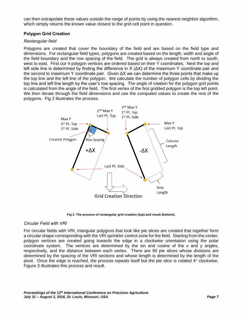
Polygons are created that cover the boundary of the field and are based on the field type and dimensions. For rectangular field types, polygons are created based on the length, width and angle of the field boundary and the row spacing of the field. The grid is always created from north to south, west to east. First our 4 polygon vertices are ordered based on their Y coordinates. Next the top and left side line is determined by finding the difference in X (ΔX) of the maximum Y coordinate pair and the second to maximum Y coordinate pair. Given ΔX we can determine the three points that make up the top line and the left line of the polygon. We calculate the number of polygon cells by dividing the top line and left line length by the user’s row spacing. The angle of rotation for the polygon grid points is calculated from the angle of the field. The first vertex of the first gridded polygon is the top left point. We then iterate through the field dimensions and use the computed values to create the rest of the polygons. Fig 2 illustrates the process.

Fig 2. The process of rectangular grid creation (top) and result (bottom).

Circular Field with VRI

For circular fields with VRI, triangular polygons that look like pie slices are created that together form a circular shape corresponding with the VRI sprinkler control zone for the field. Starting from the center, polygon vertices are created going towards the edge in a clockwise orientation using the polar coordinate system. The vertices are determined by the sin and cosine of the x and y angles, respectively, and the distance between each vertex. There are 90 pie slices whose divisions are determined by the spacing of the VRI sections and whose length is determined by the length of the pivot. Once the edge is reached, the process repeats itself but the pie slice is rotated 4° clockwise. Figure 3 illustrates this process and result.


Figure 3: The process of circular grid creation (left) and result (right).

Irregular Field and Circular Field Without VRI

For irregular fields, polygons are created similarly to a rectangular field except the point of rotation for the grid is based on the centroid of the field and the angle of rotation is based on the row orientation. If there is no row line drawn, then the grid is not rotated. The grid is also expanded +200 m of the field boundary bounding box. Fig 4 illustrates the process and result.

Fig 4. The process of irregular grid creation (left) and result (right).

Clustering of Polygon Attributes

The clustering method employed here is a univariate method of grouping based on minimizing the member deviation from the class mean while maximizing class mean deviation from other classes. It is commonly referred to as Jenks natural breaks optimization and is a well-known technique for statistical mapping (Jenks, 1967). It can also be thought of as a univariate k-means, the aforementioned clustering technique used in MZA (Dent et al., 2008). The data is first divided into arbitrary groups based on the number of classes desired and the sum of squared deviations between classes (SDBC) is calculated.


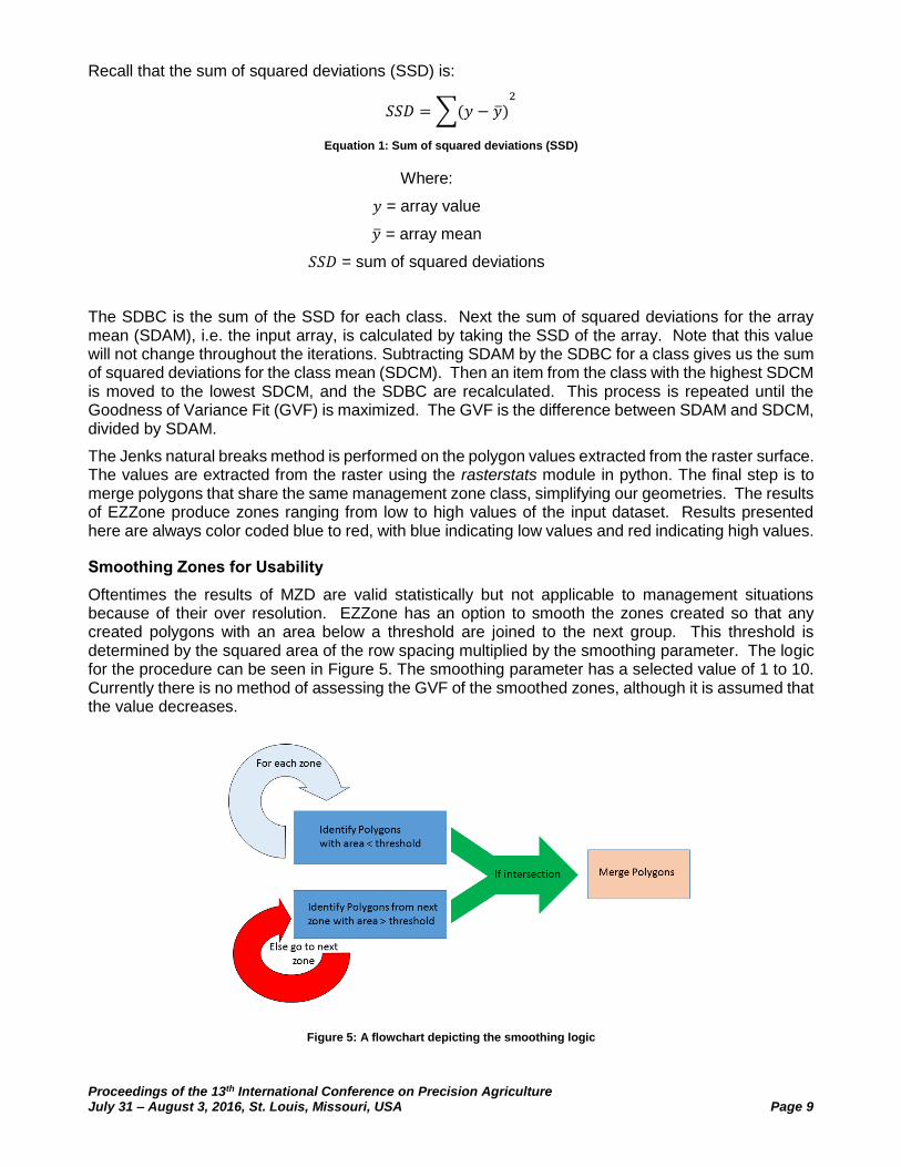
Recall that the sum of squared deviations (SSD) is:

𝑆𝑆𝐷 =∑(𝑦 − �̅�)2

Equation 1: Sum of squared deviations (SSD)

Where:

𝑦 = array value

�̅� = array mean

𝑆𝑆𝐷 = sum of squared deviations

The SDBC is the sum of the SSD for each class. Next the sum of squared deviations for the array mean (SDAM), i.e. the input array, is calculated by taking the SSD of the array. Note that this value will not change throughout the iterations. Subtracting SDAM by the SDBC for a class gives us the sum of squared deviations for the class mean (SDCM). Then an item from the class with the highest SDCM is moved to the lowest SDCM, and the SDBC are recalculated. This process is repeated until the Goodness of Variance Fit (GVF) is maximized. The GVF is the difference between SDAM and SDCM, divided by SDAM.

The Jenks natural breaks method is performed on the polygon values extracted from the raster surface. The values are extracted from the raster using the rasterstats module in python. The final step is to merge polygons that share the same management zone class, simplifying our geometries. The results of EZZone produce zones ranging from low to high values of the input dataset. Results presented here are always color coded blue to red, with blue indicating low values and red indicating high values.

Smoothing Zones for Usability

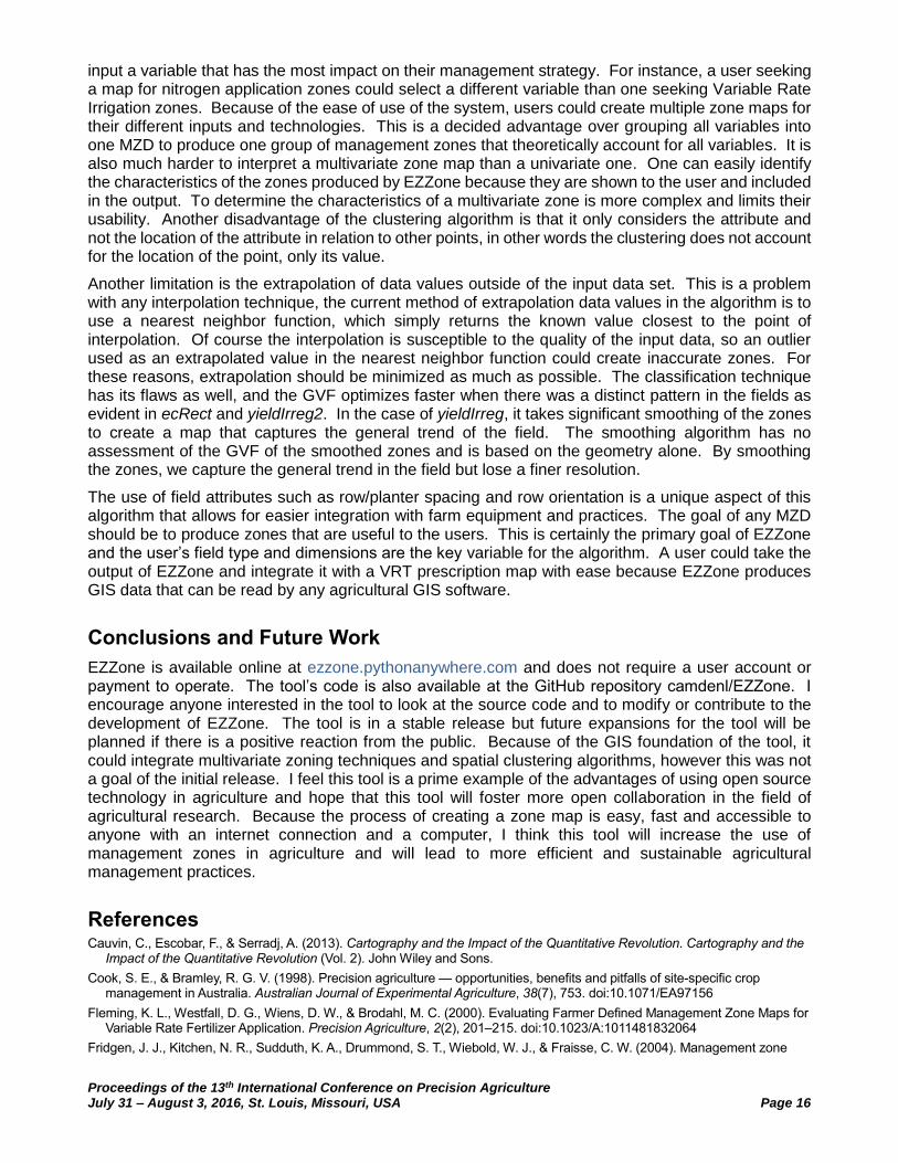
Oftentimes the results of MZD are valid statistically but not applicable to management situations because of their over resolution. EZZone has an option to smooth the zones created so that any created polygons with an area below a threshold are joined to the next group. This threshold is determined by the squared area of the row spacing multiplied by the smoothing parameter. The logic for the procedure can be seen in Figure 5. The smoothing parameter has a selected value of 1 to 10. Currently there is no method of assessing the GVF of the smoothed zones, although it is assumed that the value decreases.

Figure 5: A flowchart depicting the smoothing logic


Description of Test Datasets

All testing was done with data contributed by partner researchers. EZZone was tested on all the aforementioned field types and on two different data types -- yield and EC. The field referencing is based on the variable type, either ec or yield, and abbreviated field type, Rect, Circ, and Irreg for Rectangular, Circular with VRI and Irregular fields. Because there are two irregular fields with yield data zoned, the reference name for one of these fields has a 2 added to the end. The VRI field zoning procedure was tested on the EC values of a field in Calhoun county in southwestern Georgia located at approximately -84.55669, 31.46651 (EPSG:4326). This field is referenced as ecCirc (Fig 6, A). The rectangular field zoning procedure was tested on EC values of a vineyard outside of Volos, Greece located at approximately 22.73895, 39.26553 and referenced as ecRect (Fig 6, B). The irregular zoning procedure was tested on three different fields. The first field is located in Miller County in southwestern Georgia at approximately -84.75147, 31.17223 and EC values were used for zoning; this field is referenced as ecIrreg (Fig 6, C). The next field is located in Tift county in southwestern Georgia at approximately -83.55373, 31.51142 and cotton yield values were used; the field is referenced as yieldIrreg (Fig 6, D). The final field is located in the United Kingdom at approximately -0.45902, 52.07069. Yield data was used for this field and it is referenced as yieldIrreg2 (Fig 6, E). The summary statistics for the fields’ Z values and area are presented in Table 1.

Table 1: Summary statistics for test fields

Field Count Mean Std Dev Min Max Field Area (ha)

ecCirc 22385 9.9 5.4 0.3 56.6 85.3

ecRect 12676 73.3 20.0 8.8 114.0 1.0

ecIrreg 6298 7.8 4.2 0.4 31.3 28.8

yieldIrreg 8602 2.6 1.3 0.0 8.3 9.2

yieldIrreg2 5052 8.2 0.9 4.2 11.2 16.3


Fig 6. Test fields’ data points. A: ecCirc, B: ecRect, C: ecIrreg, D: yieldIrreg, E: yieldIrreg2

A

E

D C

B


Results and Discussion

Description of Test Procedure

EZZone was tested on each of the 5 test fields by classifying the fields until the GVF was greater than or equal to 0.8. The GVF is measured between 0 and 1 unless the classification procedure is inaccurate, in which case it will be a negative number. Because the GVF is a measurement of the homogeneity within the classes, it represents the accuracy of our classification (Cauvin, Escobar, & Serradj, 2013). It should be noted that 0.8 is an arbitrary cut off point but I feel it represents a compromise between classification optimization and a usable number of zones. EZZone allows the user to select the number of zones and recommends a number of zones based on the GVF. The zones presented here are always represented in a blue to red color scheme, blue representing low values and red representing high values.

ecCirc Classification

The ecCirc field is a central pivot field that was classified using the algorithm for VRI fields. The field exhibits marked homogeneity in the Eastern half but marked heterogeneity in the Eastern half, as evident in Fig 6, A. The field boundary was adjusted to account for large areas of the pivot span that are not planted with crops. The GVF was optimized at 4 zones with a value of .88. The resultant zones and GVF optimization can been seen in Fig 7. We can see that the zones are also largely homogeneous in the Eastern half and heterogeneous in the Western half. This indicates that the spatial variability of EC throughout the field is not static and the Western half of the field likely has very different soil attributes over a small distance. We can observe there is a general trend of low to high EC from East to West. A recommendation for the usability of these zones would be to establish a relationship between EC and the soil types of the field and then base the irrigation amount on the water holding capacity of the soil.

Fig 7. The ecCirc GVF (left) and zones (right).


ecRect classification

This field was classified using the rectangular polygon procedure, with a row spacing of 2 m. The input data for the field also seems to exhibit GPS coordinate errors because the point data does not cover the entire field. In cases like this, it is best to zone areas for which the points represent, even if the zone map doesn’t cover the entire field. While only 1 ha in size, this field had the largest standard deviation of all the fields. We can see a distinct trend in the EC values of the field from northwest to southeast. Because of this strong trend over a relatively small area, it took 3 zones to optimize the GVF and the resulting zones are very homogenous (Fig 8). This field is a good candidate for application of VRT because it is small enough that different techniques could be applied relatively easily.

ecIrreg Classification

This field has a uniquely irregular shape and there are lowland areas that are unplanted. There is little spatial homogeneity

present in the field and the EC values seem to be irregularly distributed. This results in very heterogeneous zones of the field

and the GVF optimized at 3 zones using a spacing of 2.75 m. This highlights one of the drawbacks of MZD in general. In this

case to obtain a valid statistical result, we sacrifice some readability or usability of the map. A feature unique to EZZone is the

ability to smooth the completed zones via a smoothing parameter. This allows us to take zone polygons and merge them with

larger polygons of different zones. At this point we do sacrifice some validity for the benefit of usability. The results of the

smoothed zones using a smoothing parameter of 5 are seen in Fig 9

Fig 9. The ecIrreg smoothed zones, using a smoothing parameter of 5.

Fig 8. The ecRect GVF (left) and zones (right).


Fig 9. The ecIrreg smoothed zones, using a smoothing parameter of 5

yieldIrreg Classification

The yield for a cotton field was zoned with the irregular field method although this field is somewhat rectangular (Fig 6, D). The reasoning behind this is that there were a collection of points that were completely removed from the rest of the points in the field (Fig 10, A). These are data collected by the yield monitor during calibration. EZZone’s strength lies in its visualization of the MZD process. In this case, we recognized that the produced boundary as described in 0 did not match the boundary of the field and adjusted the created boundary to match the actual boundary. In the process we are instructing EZZone to ignore those points outside of our created boundary. The GVF for yieldIrreg optimized at 4 zones and a smoothed result using a parameter of 5 is presented in Fig 11. In the middle of the field we notice that the yield is higher and exhibits a break from the trend above and below the zone (Fig 10, B). This area is actually the edge of the row and these zones are the results of edge effects in the field, where the yield is abnormally high due to increased solar radiation or sensor error. This field had no visible trend and this is reflected in the created zones.

Fig 10. The yieldIrreg calibration strip (A) and edge effects location (B).

A B


yieldIrreg2 Classification

The yield for wheat was zoned using the irregular field method and with a row spacing of 1 m. EZZone optimized the GVF in three zones. The resulting zones can be seen in Fig 12. In this field we can see large homogenous zones and a marked variability in yield in a distinct southwest to northeast trend. This field is a good candidate for VRT because of the distinct variability in yield as evident in the created zones. Considering that the yield in portions of the field is over two times greater than in other portions, this is a good opportunity to adapt strategies of site-specific management. Yield maps are arguably the primary target of zoning at least for their ability to express to farmers why VRT is important.

Fig 12. The completed yieldIrreg2 smoothed zones using a smoothing parameter of 10

Limitations and Advantages of Proposed Technique

There are limitations to the proposed technique that should be explained and evaluated. The first and foremost limitation is this EZZone is a strictly univariate technique. Limiting the technique to one variable requires the user to run the analysis more than once if more than one variable is available and leaves the user with the conundrum of how to integrate potentially different management zones resulting from each run. However, this also creates an advantage in that it encourages the user to

Fig 11. The yieldIrreg raw zones (left) and smoothed zones (right).


input a variable that has the most impact on their management strategy. For instance, a user seeking a map for nitrogen application zones could select a different variable than one seeking Variable Rate Irrigation zones. Because of the ease of use of the system, users could create multiple zone maps for their different inputs and technologies. This is a decided advantage over grouping all variables into one MZD to produce one group of management zones that theoretically account for all variables. It is also much harder to interpret a multivariate zone map than a univariate one. One can easily identify the characteristics of the zones produced by EZZone because they are shown to the user and included in the output. To determine the characteristics of a multivariate zone is more complex and limits their usability. Another disadvantage of the clustering algorithm is that it only considers the attribute and not the location of the attribute in relation to other points, in other words the clustering does not account for the location of the point, only its value.

Another limitation is the extrapolation of data values outside of the input data set. This is a problem with any interpolation technique, the current method of extrapolation data values in the algorithm is to use a nearest neighbor function, which simply returns the known value closest to the point of interpolation. Of course the interpolation is susceptible to the quality of the input data, so an outlier used as an extrapolated value in the nearest neighbor function could create inaccurate zones. For these reasons, extrapolation should be minimized as much as possible. The classification technique has its flaws as well, and the GVF optimizes faster when there was a distinct pattern in the fields as evident in ecRect and yieldIrreg2. In the case of yieldIrreg, it takes significant smoothing of the zones to create a map that captures the general trend of the field. The smoothing algorithm has no assessment of the GVF of the smoothed zones and is based on the geometry alone. By smoothing the zones, we capture the general trend in the field but lose a finer resolution.

The use of field attributes such as row/planter spacing and row orientation is a unique aspect of this algorithm that allows for easier integration with farm equipment and practices. The goal of any MZD should be to produce zones that are useful to the users. This is certainly the primary goal of EZZone and the user’s field type and dimensions are the key variable for the algorithm. A user could take the output of EZZone and integrate it with a VRT prescription map with ease because EZZone produces GIS data that can be read by any agricultural GIS software.

Conclusions and Future Work

EZZone is available online at ezzone.pythonanywhere.com and does not require a user account or payment to operate. The tool’s code is also available at the GitHub repository camdenl/EZZone. I encourage anyone interested in the tool to look at the source code and to modify or contribute to the development of EZZone. The tool is in a stable release but future expansions for the tool will be planned if there is a positive reaction from the public. Because of the GIS foundation of the tool, it could integrate multivariate zoning techniques and spatial clustering algorithms, however this was not a goal of the initial release. I feel this tool is a prime example of the advantages of using open source technology in agriculture and hope that this tool will foster more open collaboration in the field of agricultural research. Because the process of creating a zone map is easy, fast and accessible to anyone with an internet connection and a computer, I think this tool will increase the use of management zones in agriculture and will lead to more efficient and sustainable agricultural management practices.

References Cauvin, C., Escobar, F., & Serradj, A. (2013). Cartography and the Impact of the Quantitative Revolution. Cartography and the

Impact of the Quantitative Revolution (Vol. 2). John Wiley and Sons.

Cook, S. E., & Bramley, R. G. V. (1998). Precision agriculture — opportunities, benefits and pitfalls of site-specific crop management in Australia. Australian Journal of Experimental Agriculture, 38(7), 753. doi:10.1071/EA97156

Fleming, K. L., Westfall, D. G., Wiens, D. W., & Brodahl, M. C. (2000). Evaluating Farmer Defined Management Zone Maps for Variable Rate Fertilizer Application. Precision Agriculture, 2(2), 201–215. doi:10.1023/A:1011481832064

Fridgen, J. J., Kitchen, N. R., Sudduth, K. A., Drummond, S. T., Wiebold, W. J., & Fraisse, C. W. (2004). Management zone


analyst (MZA): software for subfield management zone delineation. Agronomy journal. Retrieved September 22, 2014, from http://naldc.nal.usda.gov/catalog/8380

Guastaferro, F., Castrignanò, A., de Benedetto, D., Sollitto, D., Troccoli, A., & Cafarelli, B. (2010). A comparison of different algorithms for the delineation of management zones. Precision Agriculture, 11(6), 600–620.

Katalin, T.-G., Rahoveanu, T., Magdalena, M., & István, T. (2014). Sustainable New Agricultural Technology – Economic Aspects of Precision Crop Protection. Procedia Economics and Finance, 8, 729–736. doi:10.1016/S2212-5671(14)00151-8

Lamb, D. W., Frazier, P., & Adams, P. (2008). Improving pathways to adoption: Putting the right P’s in precision agriculture. Computers and Electronics in Agriculture, 61(1), 4–9.

Lark, R. M. (1998). Forming Spatially Coherent Regions by Classification of MultiVariate Data: An Example from the Analysis of Maps of Crop Yield. International Journal of Geographical Information Science, 12(1), 83–98. doi:10.1080/136588198242021

Li, Y., Shi, Z., & Li, F. (2007). Delineation of Site-Specific Management Zones Based on Temporal and Spatial Variability of Soil Electrical Conductivity. Pedosphere. doi:10.1016/S1002-0160(07)60021-6

Li, Y., Shi, Z., Li, F., & Li, H.-Y. (2007). Delineation of site-specific management zones using fuzzy clustering analysis in a coastal saline land. Computers and Electronics in Agriculture. doi:10.1016/j.compag.2007.01.013

Moral, F. J., Terrón, J. M., & Silva, J. R. M. da. (2010). Delineation of management zones using mobile measurements of soil apparent electrical conductivity and multivariate geostatistical techniques. Soil and Tillage Research, 106(2), 335–343.

Robertson, M. J., Llewellyn, R. S., Mandel, R., Lawes, R., Bramley, R. G. V, Swift, L., … O’Callaghan, C. (2012). Adoption of variable rate fertiliser application in the Australian grains industry: Status, issues and prospects. Precision Agriculture, 13(2),

181–199.

Vellidis, G., Tucker, M., Perry, C., Kvien, C., & Bednarz, C. (2008). A real-time wireless smart sensor array for scheduling irrigation. Computers and Electronics in Agriculture, 61(1), 44–50.

Yu, P.-S. (2001). SciPy: Open source scientific tools for Python.

Zhang, N., Wang, M., & Wang, N. (2002). Precision agriculture—a worldwide overview. Computers and Electronics in Agriculture.

ezzone an online tool for delineating management zones

Documents