explicit solution to an optimal switching problem in the two‐regime case

SIAM J. CONTROL OPTIM. c© 2007 Society for Industrial and Applied MathematicsVol. 46, No. 2, pp. 395–426

EXPLICIT SOLUTION TO AN OPTIMAL SWITCHING PROBLEMIN THE TWO-REGIME CASE∗

VATHANA LY VATH† AND HUYEN PHAM†

Abstract. This paper considers the problem of determining the optimal sequence of stoppingtimes for a diffusion process subject to regime switching decisions. This is motivated in the economicsliterature by the investment problem under uncertainty for a multi-activity firm involving opening andclosing decisions. We use a viscosity solutions approach combined with the smooth-fit property, andexplicitly solve the problem in the two-regime case when the state process is of geometric Browniannature. The results of our analysis take several qualitatively different forms, depending on modelparameter values.

Key words. optimal switching, system of variational inequalities, viscosity solutions, smooth-fitprinciple

AMS subject classifications. 60G40, 49L25, 62L15

DOI. 10.1137/050638783

1. Introduction. The theory of optimal stopping and its generalization, thor-oughly studied in the 1970s, has received a renewed interest with a variety of appli-cations in economics and finance. These applications include asset pricing (Americanoptions, swing options), firm investment, and real options. We refer to [4] for aclassical and well-documented reference on the subject.

In this paper, we consider the optimal switching problem for a one-dimensionalstochastic process X. The diffusion process X may take a finite number of regimesthat are switched at stopping time decisions. For example, in the firm’s investmentproblem under uncertainty, a company (oil tanker, electricity station, etc.) managesseveral production activities operating in different modes or regimes representing anumber of different economic outlooks (e.g., state of economic growth, open or closedproduction activity). The process X is the price of input or output goods of the firmand its dynamics may differ according to the regimes. The firm’s project yields arunning payoff that depends on the commodity price X and on the regime choice.The transition from one regime to another is realized sequentially at time decisionsand incurs certain fixed costs. The problem is to find the switching strategy thatmaximizes the expected value of profits resulting from the project.

Optimal switching problems were studied by several authors; see [1] or [10]. Thesecontrol problems lead, via the dynamic programming principle, to a system of varia-tional inequalities. Applications to option pricing, real options, and investment underuncertainty were considered in [2], [5], and [7]. In this last paper, the drift andvolatility of the state process depend on an uncontrolled finite-state Markov chain,and the author provides an explicit solution to the optimal stopping problem withapplications to Russian options. In [2], an explicit solution is found for a resourceextraction problem with two regimes (open or closed field), a linear profit function,and a price process following a geometric Brownian motion. In [5], a similar model issolved with a general profit function in one regime and equal to zero in the other. In

∗Received by the editors August 24, 2005; accepted for publication (in revised form) October 24,2006; published electronically April 17, 2007.

http://www.siam.org/journals/sicon/46-2/63878.html†Laboratoire de Probabilites et Modeles Aleatoires, CNRS, UMR 7599, Universite Paris 7, 75251

Paris, Cedex 05, France ([email protected], [email protected]).

395

Dow

nloa

ded

11/3

0/14

to 1

29.1

20.2

42.6

1. R

edis

trib

utio

n su

bjec

t to

SIA

M li

cens

e or

cop

yrig

ht; s

ee h

ttp://

ww

w.s

iam

.org

/jour

nals

/ojs

a.ph

p

396 VATHANA LY VATH AND HUYEN PHAM

both models [2], [5], there is no switching in the diffusion process: changes of regimesaffect only the payoff functions. Their method of resolution is to construct a solutionto the dynamic programming system by guessing a priori the form of the strategy, andthen validate a posteriori the optimality of their candidate by a verification argument.Our model combines regime switchings on both the diffusion process and the generalprofit functions. We use a viscosity solutions approach for determining the solution tothe system of variational inequalities. In particular, we derive directly the smooth-fitproperty of the value functions and the structure of the switching regions. Explicitsolutions are provided in the following cases:

• the drift and volatility terms of the diffusion take two different regime values,and the profit functions are identical of power type;

• there is no switching on the diffusion process, and the two different profitfunctions satisfy a general condition, including typically power functions.

We also consider the cases for which both switching costs are positive, and for whichone of the two is negative. This last case is interesting in applications where a firmchooses between an open or closed activity, and may regain a fraction of its openingcosts when it decides to close. The results of our analysis take several qualitativelydifferent forms, depending on model parameter values, essentially the payoff functionsand the switching costs.

The paper is organized as follows. We formulate in section 2 the optimal switchingproblem. In section 3, we state the system of variational inequalities satisfied by thevalue functions in the viscosity sense. The smooth-fit property for this problem,proved in [9], plays an important role in our subsequent analysis. We also statesome useful properties on the switching regions. In section 4, we explicitly solvethe problem in the two-regime case when the state process is of geometric Browniannature.

2. Formulation of the optimal switching problem. We consider a stochas-tic system that can operate in d modes or regimes. The regimes can be switched ata sequence of stopping times decided by the operator (individual, firm, etc.). Theindicator of the regimes is modeled by a cadlag process It valued in Id = {1, . . . , d}.The stochastic system X (commodity price, salary, etc.) is valued in R

∗+ = (0,∞)

and satisfies the SDE.

dXt = bItXtdt + σ

ItXtdWt,(2.1)

where W is a standard Brownian motion on a filtered probability space (Ω,F ,F =(Ft)t≥0, P ) satisfying the usual conditions. bi ∈ R and σi > 0 are the drift andvolatility, respectively, of the system X once in regime It = i at time t.

A strategy decision for the operator is an impulse control α consisting of a doublesequence τ1, . . . , τn, . . . , κ1, . . . , κn, . . . , n ∈ N

∗ = N \ {0}, where τn are stoppingtimes, τn < τn+1 and τn → ∞ a.s., representing the switching regimes time decisions,and κn are Fτn-measurable valued in Id representing the new value of the regime attime t = τn. We denote by A the set of all such impulse controls. Now, for anyinitial condition (x, i) ∈ (0,∞) × Id, and any control α = (τn, κn)n≥1 ∈ A, thereexists a unique strong solution valued in (0,∞) × Id to the controlled stochasticsystem:

X0 = x, I0− = i,(2.2)

dXt = bκn

Xtdt + σκn

XtdWt, It = κn, τn ≤ t < τn+1, n ≥ 0.(2.3)

Dow

nloa

ded

11/3

0/14

to 1

29.1

20.2

42.6

1. R

edis

trib

utio

n su

bjec

t to

SIA

M li

cens

e or

cop

yrig

ht; s

ee h

ttp://

ww

w.s

iam

.org

/jour

nals

/ojs

a.ph

p

EXPLICIT SOLUTION TO OPTIMAL SWITCHING 397

Here, we set τ0 = 0 and κ0 = i. We denote by (Xx,i, Ii) this solution (as usual, weomit the dependence in α for notational simplicity). We notice that Xx,i is a contin-uous process and Ii is a cadlag process, possibly with a jump at time 0 if τ1 = 0, andso I0 = κ1.

We are given a running profit function f : R+ × Id → R and we set fi(.) = f(., i)for i ∈ Id. We assume that for each i ∈ Id, the function fi is nonnegative and isHolder continuous on R+: there exists γi ∈ (0, 1] such that (s.t.)

|fi(x) − fi(x)| ≤ C|x− x|γi ∀x, x ∈ R+,(2.4)

for some positive constant C. Without loss of generality (see Remark 2.1), we mayassume that fi(0) = 0. We also assume that for all i ∈ Id, the conjugate of fi is finiteon (0,∞):

fi(y) := supx≥0

[fi(x) − xy

]< ∞ ∀y > 0.(2.5)

The cost for switching from regime i to j is a constant equal to gij , with the conventiongii = 0, and we assume the triangular condition

gik < gij + gjk, j �= i, k.(2.6)

This last condition means that it is less expensive to switch directly in one step fromregime i to k than in two steps via an intermediate regime j. Notice that a switchingcost gij may be negative, and condition (2.6) for i = k prevents arbitrage by switchingback and forth, i.e.,

gij + gji > 0, i �= j ∈ Id.(2.7)

The expected total profit of running the system when the initial state is (x, i) andwhen using the impulse control α = (τn, κn)n≥1 ∈ A is

Ji(x, α) = E

[∫ ∞

0

e−rtf(Xx,it , Iit)dt−

∞∑n=1

e−rτngκn−1,κn

].

Here r > 0 is a positive discount factor, and we use the convention that e−rτn(ω) = 0when τn(ω) = ∞. We also make the standing assumption

r > b := maxi∈Id

bi.(2.8)

The objective is to maximize this expected total profit over all strategies α. Accord-ingly, we define the value functions

vi(x) = supα∈A

Ji(x, α), x ∈ R∗+, i ∈ Id.(2.9)

We shall see in the next section that under (2.5) and (2.8), the expectation definingJi(x) is well defined and the value function vi is finite.

Remark 2.1. The initial values fi(0) of the running profit functions receivedby the firm manager (the controller) before any decisions occur are considered tobe included in the switching costs during changing of the regime. This means that

Dow

nloa

ded

11/3

0/14

to 1

29.1

20.2

42.6

1. R

edis

trib

utio

n su

bjec

t to

SIA

M li

cens

e or

cop

yrig

ht; s

ee h

ttp://

ww

w.s

iam

.org

/jour

nals

/ojs

a.ph

p


w.l.o.g. we may assume that fi(0) = 0. Indeed, for any profit function fi, and bysetting fi = fi − fi(0), we have for all x > 0, α ∈ A,

Ji(x, α) = E

[ ∞∑n=1

∫ τn

τn−1

e−rtf(Xx,it , κn−1)dt−

∞∑n=1


]

= E

[ ∞∑n=1

∫ τn

τn−1

e−rt(f(Xx,i

t , κn−1) + fκn−1(0))dt −

∞∑n=1


]

= E

[ ∞∑n=1

∫ τn

τn−1

e−rtf(Xx,it , κn−1)dt +

fκ0(0)

r

−∞∑

n=1

e−rτn

(gκn−1,κn

+fκn(0) − fκn−1(0)

r

)]

=fi(0)

r+ E

[∫ ∞

0

e−rtf(Xx,it , Iit)dt−

∞∑n=1

e−rτn gκn−1,κn

],

with modified switching costs that take into account the possibly different initialvalues of the profit functions,

gij = gij +fj(0) − fi(0)

r,

and that are assumed to satisfy the triangle inequality gik < gij + gjk, j �= i, k.

3. System of variational inequalities, switching regions, and viscositysolutions. We first state the linear growth property and the boundary condition onthe value functions.

Lemma 3.1. We have for all i ∈ Id,

maxj∈Id

[−gij ] ≤vi(x) ≤ xy

r − b+ max

j∈Id

fj(y)

r+ max

j∈Id

[−gij ] ∀x > 0 ∀y > 0.(3.1)

In particular, we have vi(0+) = maxj∈Id

[−gij ].Proof. By considering the particular strategy α = (τn, κn) of immediately switch-

ing from the initial state (x, i) to state (x, j), j ∈ Id (eventually equal to i), at costgij and then doing nothing, i.e., τ1 = 0, κ1 = j, τn = ∞, κn = j for all n ≥ 2, wehave

Ji(x, α) = E

[∫ ∞

0

e−rtfj(Xx,jt )dt− gij

],

where Xx,j denotes the geometric Brownian in regime j starting from x at time 0.Since fj is nonnegative, and by the arbitrariness of j, we get the lower bound in (3.1).

Given an initial state (X0, I0−) = (x, i) and an arbitrary impulse control α =(τn, κn), we get from the dynamics (2.2)–(2.3) the following explicit expression ofXx,i:

Xx,it = xYt(i)

:= x

(n−1∏l=0

ebκl(τl+1−τl)Zκl

τl,τl+1

)ebκn (t−τn)Zκn

τn,t, τn ≤ t < τn+1, n ∈ N,(3.2)

Dow

nloa

ded

11/3

0/14

to 1

29.1

20.2

42.6

1. R

edis

trib

utio

n su

bjec

t to

SIA

M li

cens

e or

cop

yrig

ht; s

ee h

ttp://

ww

w.s

iam

.org

/jour

nals

/ojs

a.ph

p


where

Zjs,t = exp

(σj(Wt −Ws) −

σ2j

2(t− s)

), 0 ≤ s ≤ t, j ∈ Id.(3.3)

Here, we used the conventions that τ0 = 0, κ0 = i, and that the product term froml to n − 1 in (3.2) is equal to 1 when n = 1. We then deduce the inequality Xx,i

t ≤xebtMt for all t, where

Mt =

(n−1∏l=0

Zκlτl,τl+1

)Zκnτn,t, τn ≤ t < τn+1, n ∈ N.(3.4)

Now, we notice that (Mt) is a martingale obtained by continuously patching themartingales (Z

κn−1

τn−1,t) and (Zκnτn,t) at the stopping times τn, n ≥ 1. In particular, we

have E[Mt] = M0 = 1 for all t.We set f(y) = maxj∈Id

fi(y), y > 0, and we notice by definition of fi in (2.5) that

f(Xx,it , Iit) ≤ yXx,i

t + f(y) for all t, y. Moreover, we show by induction on N that forall N ≥ 1, τ1 ≤ · · · ≤ τN , κ0 = i, κn ∈ Id, n = 1, . . . , N ,

−N∑

n=1


≤ maxj∈Id

[−gij ] a.s.

Indeed, the above assertion is obviously true for N = 1. Suppose now it holds trueat step N . Then, at step N + 1, we distinguish two cases:

• If gκN,κN+1≥ 0, then we have −

∑N+1n=1 e−rτngκn−1,κn

≤ −∑N

n=1 e−rτngκn−1,κn

and we conclude by the induction hypothesis at step N .• If g

κN,κN+1< 0, then by (2.6), and since τN ≤ τN+1, we have −e−rτN g

κN−1,κN−

e−rτN+1gκN,κN+1

≤ e−rτN gκN−1,κN+1

, and so −∑N+1

n=1 e−rτngκn−1,κn

≤−∑N

n=1 e−rτng

κn−1,κn, with κn = κn for n = 1, . . . , N − 1, κN = κN+1.

We then conclude by the induction hypothesis at step N .It follows that

Ji(x, α) ≤ E

[∫ ∞

0

e−rt(yxebtMt + f(y)

)dt + max

j∈Id

[−gij ]

]

=

∫ ∞

0

e−(r−b)tyxE[Mt]dt +

∫ ∞

0

e−rtf(y)dt + maxj∈Id

[−gij ]

=xy

r − b+

f(y)

r+ max

j∈Id

[−gij ].

From the arbitrariness of α, this shows the upper bound for vi.By sending x to zero and then y to infinity into the r.h.s. of (3.1), and recalling

that fi(∞) = fi(0) = 0 for i ∈ Id, we conclude that vi goes to maxj∈Id[−gij ] when x

tends to zero.We next show the Holder continuity of the value functions.Lemma 3.2. For all i ∈ Id, vi is Holder continuous on (0,∞):

|vi(x) − vi(x)| ≤ C|x− x|γ ∀x, x ∈ (0,∞) with |x− x| ≤ 1,

for some positive constant C, and where γ = mini∈Idγi of condition (2.4).

Dow

nloa

ded

11/3

0/14

to 1

29.1

20.2

42.6

1. R

edis

trib

utio

n su

bjec

t to

SIA

M li

cens

e or

cop

yrig

ht; s

ee h

ttp://

ww

w.s

iam

.org

/jour

nals

/ojs

a.ph

p


Proof. By definition (2.9) of vi and under condition (2.4), we have for all x, x ∈(0,∞), with |x− x| ≤ 1,

|vi(x) − vi(x)| ≤ supα∈A

|Ji(x, α) − Ji(x, α)|

≤ supα∈A

E

[∫ ∞

0

e−rt∣∣∣f(Xx,i

t , Iit) − f(X x,it , Iit)

∣∣∣ dt]

≤ C supα∈A

E

[∫ ∞

0

e−rt∣∣∣Xx,i

t −X x,it

∣∣∣γIit dt

]

= C supα∈A

∫ ∞

0

E[e−rt|x− x|γIit |Yt(i)|

γIit dt

]≤ C|x− x|γ sup

α∈A

∫ ∞

0

e−(r−b)tE|Mt|γIit dt(3.5)

by (3.2) and (3.4). For any α = (τn, κn)n ∈ A, by the independence of (Zκnτn,τn+1

)n in(3.3), and since

E[∣∣∣Zκn

τn,τn+1

∣∣∣γκn∣∣∣Fτn

]= E

[exp

(γκn(γκn − 1)

σ2κn

2(τn+1 − τn)

)∣∣∣∣Fτn

]≤ 1 a.s.,

we clearly see that E|Mt|γIit ≤ 1 for all t ≥ 0. We thus conclude with (3.5).

The dynamic programming principle combined with the notion of viscosity solu-tions is known to be a general and powerful tool for characterizing the value functionof a stochastic control problem via a PDE representation; see [6]. We recall thedefinition of viscosity solutions for a PDE in the form

H(x, v,Dxv,D2xxv) = 0, x ∈ O,(3.6)

where O is an open subset in Rn and H is a continuous function and nonincreasing

in its last argument (with respect to the order of symmetric matrices).Definition 3.3. Let v be a continuous function on O. We say that v is a

viscosity solution to (3.6) on O if it is(i) a viscosity supersolution to (3.6) on O: For any x ∈ O and any C2 function

ϕ in a neighborhood of x s.t. x is a local minimum of v − ϕ, we have

H(x, v(x), Dxϕ(x), D2xxϕ(x)) ≥ 0;

and(ii) a viscosity subsolution to (3.6) on O: For any x ∈ O and any C2 function ϕ

in a neighborhood of x s.t. x is a local maximum of v − ϕ, we have

H(x, v(x), Dxϕ(x), D2xxϕ(x)) ≤ 0.

Remark 3.1. 1. By misuse of notation, we shall say that v is a viscosity superso-lution (resp., subsolution) to (3.6) by writing

H(x, v,Dxv,D2xxv) ≥ (resp., ≤) 0, x ∈ O,(3.7)

2. We recall that if v is a smooth C2 function on O, supersolution (resp., sub-solution) in the classical sense to (3.7), then v is a viscosity supersolution (resp.,subsolution) to (3.7).

Dow

nloa

ded

11/3

0/14

to 1

29.1

20.2

42.6

1. R

edis

trib

utio

n su

bjec

t to

SIA

M li

cens

e or

cop

yrig

ht; s

ee h

ttp://

ww

w.s

iam

.org

/jour

nals

/ojs

a.ph

p


3. There is an equivalent formulation of viscosity solutions, which is useful forproving uniqueness results (see [3]).

(i) A continuous function v on O is a viscosity supersolution to (3.6) if

H(x, v(x), p,M) ≥ 0 ∀x ∈ O, ∀(p,M) ∈ J2,−v(x).

(ii) A continuous function v on O is a viscosity subsolution to (3.6) if

H(x, v(x), p,M) ≤ 0 ∀x ∈ O, ∀(p,M) ∈ J2,+v(x).

Here J2,+v(x) is the second order superjet defined by

J2,+v(x) =

⎧⎨⎩(p,M) ∈ R

n × Sn :

lim supx′ → xx ∈ O

v(x′) − v(x) − p.(x′ − x) − 12 (x′ − x).M(x′ − x)

|x′ − x|2 ≤ 0

⎫⎬⎭ ,

Sn is the set of symmetric n× n matrices, and J2,−v(x) = −J2,+(−v)(x).In what follows, we shall denote by Li the second order operator associated with

the diffusion X when we are in regime i: for any C2 function ϕ on (0,∞),

Liϕ =1

2σ2i x

2ϕ′′ + bixϕ′.

We then have the following PDE characterization of the value functions vi bymeans of viscosity solutions.

Theorem 3.4. The value functions vi, i ∈ Id, are the unique viscosity so-lutions, with linear growth conditions on (0,∞) and boundary conditions vi(0

+) =maxj∈Id

[−gij ], to the system of variational inequalities:

min

{rvi − Livi − fi , vi − max

j �=i(vj − gij)

}= 0, x ∈ (0,∞), i ∈ Id.(3.8)

This means we have the following properties.(1) Viscosity property. For each i ∈ Id, vi is a viscosity solution to

min

{rvi − Livi − fi , vi − max

j �=i(vj − gij)

}= 0, x ∈ (0,∞).(3.9)

(2) Uniqueness property. If wi, i ∈ Id, are viscosity solutions, with linear growthconditions on (0,∞) and boundary conditions wi(0

+) = maxj∈Id[−gij ], to the system

of variational inequalities (3.8), then vi = wi on (0,∞).Proof. (1) The viscosity property follows from the dynamic programming principle

and is proved in [9].(2) Uniqueness results for switching problems have been proved in [10] in the finitehorizon case under different conditions. For sake of completeness, we provide in theappendix a proof of the comparison principle in our infinite horizon context, whichimplies the uniqueness result.

Remark 3.2. For fixed i ∈ Id, we also have uniqueness of viscosity solutions to(3.9) in the class of continuous functions with linear growth conditions on (0,∞) and

Dow

nloa

ded

11/3

0/14

to 1

29.1

20.2

42.6

1. R

edis

trib

utio

n su

bjec

t to

SIA

M li

cens

e or

cop

yrig

ht; s

ee h

ttp://

ww

w.s

iam

.org

/jour

nals

/ojs

a.ph

p


given boundary conditions on 0. In the next section, we shall use either uniquenessof viscosity solutions to the system (3.8) or for fixed i to (3.9), for the identificationof an explicit solution in the two-regime case d = 2.

We shall also combine the uniqueness result for the viscosity solutions with thesmooth-fit property on the value functions that we state below.

For any regime i ∈ Id, we introduce the switching region

Si =

{x ∈ (0,∞) : vi(x) = max

j �=i(vj − gij)(x)

}.

Si is a closed subset of (0,∞) and corresponds to the region where it is optimal forthe operator to change regime. The complement set Ci of Si in (0,∞) is the so-calledcontinuation region:

Ci =

{x ∈ (0,∞) : vi(x) > max

j �=i(vj − gij)(x)

},

where the operator remains in regime i. In this open domain, the value function vi issmooth C2 on Ci and satisfies, in a classical sense,

rvi(x) − Livi(x) − fi(x) = 0, x ∈ Ci.

As a consequence of the condition (2.6), we have the following elementary partitionproperty of the switching regions (see Lemma 4.2 in [9]):

Si = ∪j �=iSij , i ∈ Id,

where

Sij = {x ∈ Cj : vi(x) = (vj − gij)(x)} .

Sij represents the region where it is optimal to switch from regime i to regime j and toremain for a moment, i.e., without changing instantaneously from regime j to anotherregime. The following lemma gives some partial information about the structure ofthe switching regions.

Lemma 3.5. For all i �= j in Id, we have

Sij ⊂ Qij := {x ∈ Cj : (Lj − Li)vj(x) + (fj − fi)(x) − rgij ≥ 0} .

Proof. Let x ∈ Sij . By setting ϕj = vj − gij , this means that x is a minimumof vi − ϕj with vi(x) = ϕj(x). Moreover, since x lies in the open set Cj where vj issmooth, we have that ϕj is C2 in a neighborhood of x. By the supersolution viscosityproperty of vi to the PDE (3.8), this yields

rϕj(x) − Liϕj(x) − fi(x) ≥ 0.(3.10)

Now recall that for x ∈ Cj , we have

rvj(x) − Ljvj(x) − fj(x) = 0,

so that by substituting into (3.10), we obtain

(Lj − Li)vj(x) + (fj − fi)(x) − rgij ≥ 0,

Dow

nloa

ded

11/3

0/14

to 1

29.1

20.2

42.6

1. R

edis

trib

utio

n su

bjec

t to

SIA

M li

cens

e or

cop

yrig

ht; s

ee h

ttp://

ww

w.s

iam

.org

/jour

nals

/ojs

a.ph

p


which is the required result.We quote the smooth-fit property on the value functions, proved in [9].Theorem 3.6. For all i ∈ Id, the value function vi is continuously differentiable

on (0,∞).Remark 3.3. In a given regime i, the variational inequality satisfied by the value

function vi is a free-boundary problem as in the optimal stopping problem, whichdivides the state space into the switching region (stopping region in the pure optimalstopping problem) and the continuation region. The main difficulty with regard tooptimal stopping problems for proving the smooth-fit property through the bound-aries of the switching regions, is that the switching region for the value function videpends also on the other value functions vj . The method in [9] uses viscosity so-lutions arguments, and the condition of one-dimensional state space is critical forproving the smooth-fit property. The crucial conditions in this paper require that thediffusion coefficient in any regime of the system X be strictly positive on the interiorof the state space, which is the case here since σi > 0 for all i ∈ Id, and a triangularcondition (2.6) on the switching costs. Under these conditions, on a point x of theswitching region Si for regime i, there exists some j �= i s.t. x ∈ Sij , i.e., vi(x) =vj(x) − gij , and the C1 property of the value functions is written as v′i(x) = v′j(x)since gij is constant.

The next result provides suitable conditions for determining a viscosity solutionto the variational inequality type arising in our switching problem.

Lemma 3.7. Fix i ∈ Id. Let C be an open set in (0,∞), S = (0,∞)\C assumed tobe the union of a finite number of closed intervals in (0,∞), and w, h two continuousfunctions on (0,∞), with w = h on S such that

w is C1 on ∂S,(3.11)

w ≥ h on C,(3.12)

w is C2 on C, solution to

rw − Liw − fi = 0 on C,(3.13)

and w is a viscosity supersolution to

rw − Liw − fi ≥ 0 on int(S).(3.14)

Here int(S) is the interior of S and ∂S = S \ int(S) its boundary. Then, w is aviscosity solution to

min {rw − Liw − fi, w − h} = 0 on (0,∞).(3.15)

Proof. Take some x ∈ (0,∞) and distinguish the following cases:• x ∈ C. Since w = v is C2 on C and satisfies rw(x) − Liw(x) − fi(x) = 0 by

(3.13), and recalling w(x) ≥ h(x) by (3.12), we obtain the classical solution property,and so a fortiori the viscosity solution property (3.15) of w at x.

• x ∈ S. Then w(x) = h(x) and the viscosity subsolution property is trivial atx. It remains to show the viscosity supersolution property at x. If x ∈ int(S), thisfollows directly from (3.14). Suppose now x ∈ ∂S, and to fix the idea, we considerthat x is on the left-boundary of S so that from the assumption on the form of S,there exists ε > 0 s.t. (x − ε, x) ⊂ C on which w is smooth C2 (the same argumentholds true when x is on the right-boundary of S). Take some smooth C2 function ϕ

Dow

nloa

ded

11/3

0/14

to 1

29.1

20.2

42.6

1. R

edis

trib

utio

n su

bjec

t to

SIA

M li

cens

e or

cop

yrig

ht; s

ee h

ttp://

ww

w.s

iam

.org

/jour

nals

/ojs

a.ph

p


s.t. x is a local minimum of w − ϕ. Since w is C1 by (3.11), we have ϕ′(x) = w′(x).We may also assume w.l.o.g. (by taking ε small enough) that (w−ϕ)(x) ≤ (w−ϕ)(x)for x ∈ (x− ε, x). Moreover, by Taylor’s formula, we have

w(x− η) = w(x) − η

∫ 1

0

w′(x− tη)dt,ϕ(x− η) = ϕ(x) − η

∫ 1

0

ϕ′(x− tη)dt,

so that ∫ 1

0

ϕ′(x− tη) − w′(x− tη) dt ≥ 0 ∀ 0 < η < ε.

Since ϕ′(x) = w′(x), this last inequality is written as∫ 1

0

ϕ′(x− tη) − ϕ′(x)

η− w′(x− tη) − w′(x)

ηdt ≥ 0 ∀ 0 < η < ε.(3.16)

Now, from (3.13), we have rw(x)−Liw(x)− fi(x) = 0 for x ∈ (x− ε, x). By sendingx towards x into this last equality, this shows that w′′(x−) = limx↗x w

′′(x) exists,and

rw(x) − bixw′(x) − 1

2σ2i x

2w′′(x−) − fi(x) = 0.(3.17)

Moreover, by sending η to zero into (3.16), we obtain∫ 1

0

t[− ϕ′′(x) + w′′(x−)

]dt ≥ 0,

and so ϕ′′(x) ≤ w′′(x−). By substituting into (3.17), and recalling that w′(x) = ϕ′(x),we then obtain

rw(x) − Liϕ(x) − fi(x) ≥ 0,

which is the required supersolution inequality and ends the proof.Remark 3.4. Since w = h on S, relation (3.14) means equivalently that h is a

viscosity supersolution to

rh− Lih− fi ≥ 0 on int(S).(3.18)

Practically, Lemma 3.7 shall be used as follows in the next section: We consider twoC1 functions v and h on (0,∞) s.t.

v(x) = h(x), v′(x) = h′(x), x ∈ ∂S,v ≥ h on C,

v is C2 on C, solution to

rv − Liv − fi = 0 on C,

and h is a viscosity supersolution to (3.18). Then, the function w defined on (0,∞)by

w(x) =

{v(x), x ∈ C,h(x), x ∈ S

Dow

nloa

ded

11/3

0/14

to 1

29.1

20.2

42.6

1. R

edis

trib

utio

n su

bjec

t to

SIA

M li

cens

e or

cop

yrig

ht; s

ee h

ttp://

ww

w.s

iam

.org

/jour

nals

/ojs

a.ph

p


satisfies the conditions of Lemma 3.7 and is a viscosity solution to (3.15). This lemmacombined with uniqueness viscosity solution results may be viewed as an alternative tothe classical verification approach in the identification of the value function. Moreover,with our viscosity solutions approach, we shall see in section 4.2 that Lemma 3.5and the smooth-fit property of the value functions in Theorem 3.6 provide a directderivation for the structure of the switching regions, and thus of the solution to ourproblem.

4. Explicit solution in the two-regime case. In this section, we consider thecase where d = 2. In this two-regime case, we know from Theorem 3.4 that the valuefunctions vi, i = 1, 2, are the unique continuous viscosity solutions, with linear growthconditions on (0,∞), and boundary conditions vi(0

+) = (−gij)+ := max(−gij , 0), j�= i, to the system

min {rv1 − L1v1 − f1, v1 − (v2 − g12)} = 0,(4.1)

min {rv2 − L2v2 − f2, v2 − (v1 − g21)} = 0.(4.2)

Moreover, the switching regions are

Si = Sij = {x > 0 : vi(x) = vj(x) − gij} , i, j = 1, 2, i �= j.

We set

x∗i = inf Si ∈ [0,∞]x∗

i = supSi ∈ [0,∞],

with the usual convention that inf ∅ = ∞.Let us also introduce some other notation. We consider the second order ODE

for i = 1, 2:

rv − Liv − fi = 0,(4.3)

whose general solution (without second member fi) is given by

v(x) = Axm+i + Bxm−

i ,

for some constants A, B, and where

m−i = − bi

σ2i

+1

2−

√(− biσ2i

+1

2

)2

+2r

σ2i

< 0,

m+i = − bi

σ2i

+1

2+

√(− biσ2i

+1

2

)2

+2r

σ2i

> 1.

We also denote

Vi(x) = E

[∫ ∞

0

e−rtfi(Xx,it )dt

],

with Xx,i the solution to the SDE dXt = biXtdt + σiXtdWt, X0 = x. Actually, Vi

is a particular solution to ODE (4.3), with boundary condition Vi(0+) = fi(0) = 0.

It corresponds to the reward function associated with the no switching strategy frominitial state (x, i), and so Vi ≤ vi.

Dow

nloa

ded

11/3

0/14

to 1

29.1

20.2

42.6

1. R

edis

trib

utio

n su

bjec

t to

SIA

M li

cens

e or

cop

yrig

ht; s

ee h

ttp://

ww

w.s

iam

.org

/jour

nals

/ojs

a.ph

p


Remark 4.1. If gij > 0, then from (2.7), we have vi(0+) = 0 > (−gji)+ − gij =

vj(0+)−gij . Therefore, by continuity of the value functions on (0,∞), we get x∗

i > 0.We now give the explicit solution to our problem in the following two situations:• The diffusion operators are different and the running profit functions are

identical.• The diffusion operators are identical and the running profit functions are

different.We also consider the cases for which both switching costs are positive, and for

which one of the two is negative, the other being then positive according to (2.7).This last case is interesting in applications where a firm chooses between an open orclosed activity, and may regain a fraction of its opening costs when it decides to close.

4.1. Identical profit functions with different diffusion operators. In thissubsection, we suppose that the running functions are identical in the form

f1(x) = f2(x) = xγ , 0 < γ < 1,(4.4)

and the diffusion operators are different. A straightforward calculation shows thatunder (4.4), we have

Vi(x) = Kixγ with Ki =

1

r − biγ + 12σ

2i γ(1 − γ)

> 0, i = 1, 2.

We show that the structure of the switching regions depends actually only on thesign of K2 −K1, and of the sign of the switching costs g12 and g21. More precisely,we have the following explicit result.

Theorem 4.1. Let i, j = 1, 2, i �= j.(1) If Ki = Kj, then

vi(x) = Vi(x) + (−gij)+, x ∈ (0,∞),

Si =

{∅ if gij > 0,

(0,∞) if gij ≤ 0.

It is always optimal to switch from regime i to j if the corresponding switching cost isnonpositive, and never optimal to switch otherwise.

(2) If Kj > Ki, then we have the following situations depending on the switchingcosts:

(a) gij ≤ 0: We have Si = (0,∞), Sj = ∅, and

vi = Vj − gij ,vj = Vj .

(b) gij > 0:• If gji ≥ 0, then Si = [x∗

i ,∞) with x∗i ∈ (0,∞), Sj = ∅, and

vi(x) =

{Axm+

i + Vi(x), x < x∗i ,

vj(x) − gij , x ≥ x∗i ,

(4.5)

vj(x) = Vj(x), x ∈ (0,∞),(4.6)

where the constants A and x∗i are determined by the continuity and

smooth-fit conditions of vi at x∗i , and explicitly given by

x∗i =

(m+

i

m+i − γ

gijKj −Ki

) 1γ

,(4.7)

A = (Kj −Ki)γ

m+i

(x∗i )

γ−m+i .(4.8)

Dow

nloa

ded

11/3

0/14

to 1

29.1

20.2

42.6

1. R

edis

trib

utio

n su

bjec

t to

SIA

M li

cens

e or

cop

yrig

ht; s

ee h

ttp://

ww

w.s

iam

.org

/jour

nals

/ojs

a.ph

p


When we are in regime i, it is optimal to switch to regime j wheneverthe state process X exceeds the threshold x∗

i , while when we are in regimej, it is optimal to never switch.

• If gji < 0, then Si = [x∗i ,∞) with x∗

i ∈ (0,∞), Sj = (0, x∗j ], and

vi(x) =

{Axm+

i + Vi(x), x < x∗i ,

vj(x) − gij , x ≥ x∗i ,

(4.9)

vj(x) =

{vi(x) − gji, x ≤ x∗

j ,

Bxm−j + Vj(x), x > x∗

i ,(4.10)

where the constants A, B and x∗j < x∗

i are determined by the continuityand smooth-fit conditions of vi and vj at x∗

i and x∗j , and explicitly given

by

xj =

[−m−

j (gji + gijym

+i )

(Ki −Kj)(γ −m−j )(1 − ym

+i −γ)

] 1γ

,

xi=

xj

y,

B =(Ki −Kj)(m

+i − γ)x

γ−m−j

i + m+i gijx

−mji

m+i −m−

j

,

A = Bxm−

j −m+i

i − (Ki −Kj)xγ−m+

ii

− gijx−m+

ii

,

with y solution in (0,

(−gji

gij

) 1

m+i

)

to the equation

m+i (γ −m−

j )(1 − ym

+i −γ

)(gijy

m−j + g

ji

)+ m−

j (m+i − γ)

(1 − ym

−j −γ

)(gijy

m+i + gji

)= 0.

When we are in regime i, it is optimal to switch to regime j wheneverthe state process X exceeds the threshold x∗

i , while when we are in regimej, it is optimal to switch to regime i for values of the state process Xunder the threshold x∗

j .

Economic interpretation. In the particular case where σ1 = σ2, we have thatK2 − K1 > 0 means that regime 2 provides a higher expected return b2 than b1 ofregime 1 for the same volatility coefficient σi. Moreover, if the switching cost g21 fromregime 2 to regime 1 is nonnegative, it is intuitively clear that it is in our best interestto always stay in regime 2, which is formalized by the property that S

2= ∅. However,

if one receives some gain compensation to switch from regime 2 to regime 1, i.e., thecorresponding cost g

21 is negative, then it is in our best interest to change regime forsmall values of the current state. This is formalized by the property that S2 = (0, x∗

2].On the other hand, in regime 1, our best interest is to switch to regime 2, for all current

Dow

nloa

ded

11/3

0/14

to 1

29.1

20.2

42.6

1. R

edis

trib

utio

n su

bjec

t to

SIA

M li

cens

e or

cop

yrig

ht; s

ee h

ttp://

ww

w.s

iam

.org

/jour

nals

/ojs

a.ph

p


22 Vv

x

x

continue

0g0,g,KK,ff:I.1.aFigure 21122121

continue

2Regime

1Regime11 Vv x

x

2112 gVv

0g0,g,KK,ff:I.1.bFigure 21122121

continue

switch

11 Vv

2Regime

1Regime

x

x2Regime

1Regime

continue

1221 gVvswitch

22 Vv

0g,KK,ff:I.2.aFigure 121221

x

x2Regime

1Regime

continue

switchcontinue

22 Vv

0g0,g,KK,ff:I.2.biFigure 21121221

1m

1 VAxv 1 1221 gVv*1x

x

x2Regime

1Regime*1x

continue

continue

*2x

switch

switch

0g0,g,KK,ff:I.2.biiFigure 21121221

Fig. 1.

values of the state if the corresponding switching cost g12 is nonpositive, or from acertain threshold x∗

1 if the switching cost g12 is positive. A similar interpretation holdswhen b1 = b2, and K2 −K1 > 0, i.e., σ2 < σ1. Theorem 4.1 extends these results forgeneral coefficients bi and σi, and shows that the critical parameter value determiningthe form of the optimal strategy is given by the sign of K2 − K1 and the switchingcosts. The different optimal strategy structures are depicted in Figure 1.

Proof of Theorem 4.1.(1) If Ki = Kj , then Vi = Vj . We consider the smooth functions wi = Vi+(−gij)+

for i, j = 1, 2 and j �= i. Since Vi are solutions to (4.3), we see that wi satisfy

rwi − Lwi − fi = r(−gij)+,(4.11)

wi − (wj − gij) = gij + (−gij)+ − (−gji)+.(4.12)

Notice that the l.h.s. of (4.11) and (4.12) are both nonnegative by (2.7). Moreover,

Dow

nloa

ded

11/3

0/14

to 1

29.1

20.2

42.6

1. R

edis

trib

utio

n su

bjec

t to

SIA

M li

cens

e or

cop

yrig

ht; s

ee h

ttp://

ww

w.s

iam

.org

/jour

nals

/ojs

a.ph

p


if gij > 0, then the l.h.s. of (4.11) is zero, and if gij ≤ 0, then gji > 0 and the l.h.s.of (4.12) is zero. Therefore, wi, i = 1, 2 is solution to the system

min {rwi − Liwi − fi, wi − (wj − gij)} = 0.

Since Vi(0+) = 0, we have wi(0

+) = (−gij)+. Moreover, wi like Vi satisfies a lineargrowth condition. Therefore, from the uniqueness solutions to the PDE system (4.1)–(4.2), we deduce that vi = wi. As observed above, if gij ≤ 0, then the l.h.s. of (4.12)is zero, and so Si = (0,∞). Finally, if gij > 0, then the l.h.s. of (4.12) is positive, andso Si = ∅.

(2) We now suppose w.l.o.g. that K2 > K1.(a) Consider first the case where g

12≤ 0, and so g

21> 0. We set w1 =

V2 − g12 and w2 = V2. Then, by construction, we have w1 = w2 − g12

on (0,∞), andby definition of V1 and V2:

rw1(x) − L1w1(x) − f1(x) =K2 −K1

K1xγ − rg

12 > 0 ∀ x > 0.

On the other hand, we also have rw2 −L2w2 − f2 = 0 on (0,∞), and w2 ≥ w1 − g21

since g12

+ g21

≥ 0. Hence, w1 and w2 are smooth (hence, viscosity) solutions to thesystem (4.1)–(4.2), with linear growth conditions and boundary conditions w1(0

+) =V1(0

+) − g12 = (−g12)+, w2(0+) = V2(0

+) = 0 = (−g21)+. By the uniqueness resultof Theorem 3.4, we deduce that v1 = w1, v2 = w2, and thus S1 = (0,∞), S2 = ∅.

(b) Consider now the case where g12

> 0. We already know from Remark 4.1that x∗

1> 0, and we claim that x∗

1< ∞. Otherwise, v1 should be equal to V1 . Since

v1 ≥ v2 − g12 ≥ V2 − g12 , this would imply (V2 − V1)(x) = (K2 −K1)x

γ ≤ g12 for allx > 0, an obvious contradiction. By definition of x∗

1, we have (0, x∗

1) ⊂ C1. We shallprove actually the equality (0, x∗

1) = C1, i.e., S1 = [x∗

1,∞). On the other hand, the

form of S2 will depend on the sign of g21 .Case: g

21 ≥ 0.We shall prove that C2 = (0,∞), i.e., S2 = ∅. To this end, let us consider the

function

w1(x) =

{Axm+

1 + V1(x), 0 < x < x1 ,

V2(x) − g12 , x ≥ x1 ,

where the positive constants A and x1 satisfy

Axm+1

1+ V1(x1) = V2(x1) − g12 ,(4.13)

Am+1 x

m+1 −1

1+ V ′

1(x1) = V ′

2(x1),(4.14)

and are explicitly determined by

(K2 −K1)xγ1

=m+

1

m+1 − γ

g12 ,(4.15)

A = (K2 −K1)γ

m+1

xγ−m+1

1.(4.16)

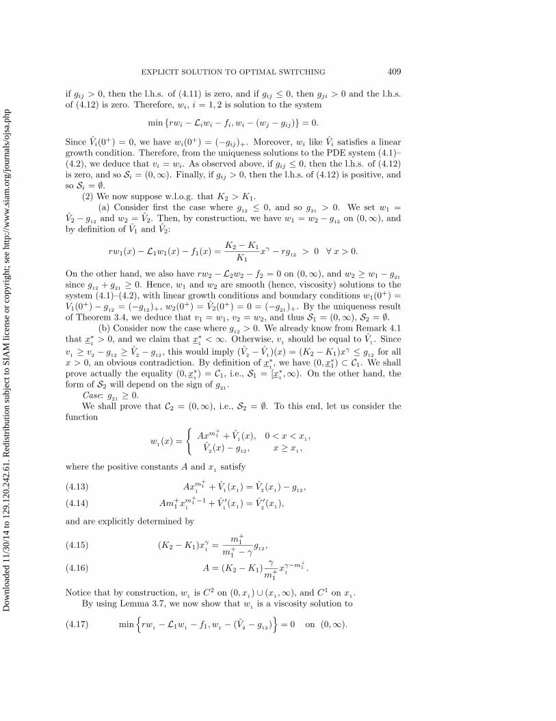
Notice that by construction, w1 is C2 on (0, x1) ∪ (x1 ,∞), and C1 on x1 .By using Lemma 3.7, we now show that w1 is a viscosity solution to

min{rw

1 − L1w1 − f1, w1 − (V2− g12)

}= 0 on (0,∞).(4.17)

Dow

nloa

ded

11/3

0/14

to 1

29.1

20.2

42.6

1. R

edis

trib

utio

n su

bjec

t to

SIA

M li

cens

e or

cop

yrig

ht; s

ee h

ttp://

ww

w.s

iam

.org

/jour

nals

/ojs

a.ph

p


We first check that

w1(x) ≥ V2(x) − g12 ∀ 0 < x < x1 ,(4.18)

i.e.,

G(x) := Axm+1 + V

1(x) − V

2(x) + g

12≥ 0 ∀ 0 < x < x

1.

Since A > 0, 0 < γ < 1 < m+1 , K2−K1 > 0, a direct derivation shows that the second

derivative of G is positive, i.e., G is strictly convex. By (4.14), we have G′(x1) = 0,and so G′ is negative, i.e., G is strictly decreasing on (0, x1). Now, by (4.13), we haveG(x

1) = 0, and thus G is positive on (0, x

1), which proves (4.18).

By definition of w1 on (0, x1), we have in the classical sense

rw1 − L1w1 − f1 = 0 on (0, x1).(4.19)

We now check that

rw1− L1w1

− f1 ≥ 0 on (x1,∞)(4.20)

holds true in the classical sense, and so a fortiori in the viscosity sense. By definitionof w1 on (x1 ,∞), and K1, we have for all x > x1 ,

rw1(x) − L1w1(x) − f1(x) =K2 −K1

K1xγ − rg12 ∀x > x

1 ,

so that (4.20) is satisfied iff K2−K1

K1xγ

1− rg

12≥ 0, or equivalently by (4.15),

m+1

m+1 − γ

≥ rK1 =r

r − b1γ + 12σ

21γ(1 − γ)

.(4.21)

Now, since γ < 1 < m+1 , and by definition of m+

1 , we have

1

2σ2

1m+1 (γ − 1) <

1

2σ2

1m+1 (m+

1 − 1) = r − b1m+1 ,

which proves (4.21) and thus (4.20).Relations (4.13)–(4.14) and (4.18)–(4.20) mean that the conditions of Lemma 3.7

are satisfied with C = (0, x1), h = V2 − g12 , and we thus get the required assertion

(4.17).On the other hand, we check that

V2(x) ≥ w1(x) − g21 ∀x > 0,(4.22)

which amounts to showing

H(x) := Axm+1 + V1(x) − V2(x) − g21 ≤ 0 ∀ 0 < x < x1 .

Since A > 0, 0 < γ < 1 < m+1 , K2−K1 > 0, a direct derivation shows that the second

derivative of H is positive, i.e., H is strictly convex. By (4.14), we have H ′(x1) = 0and so H ′ is negative, i.e., H is strictly decreasing on (0, x1). Now, we have H(0) =−g21

≤ 0 and thus H is negative on (0, x1), which proves (4.22). Recalling that V

2is

Dow

nloa

ded

11/3

0/14

to 1

29.1

20.2

42.6

1. R

edis

trib

utio

n su

bjec

t to

SIA

M li

cens

e or

cop

yrig

ht; s

ee h

ttp://

ww

w.s

iam

.org

/jour

nals

/ojs

a.ph

p


a solution to rV2− L2V2

− f2 = 0 on (0,∞), we deduce that, obviously from (4.22),V

2 is a classical, hence a viscosity, solution to

min{rV2 − L2V2 − f2, V2 − (w1 − g21)

}= 0 on (0,∞).(4.23)

Since w1(0

+) = 0 = (−g12)+, V2(0+) = 0 = (−g21)+, and w1 , V2 satisfy a linear

growth condition, we deduce from (4.17), (4.23), and uniqueness to the PDE system(4.1)–(4.2) that

v1 = w1,v

2= V

2on (0,∞).

This proves x∗1

= x1 , S1 = [x1,∞), and S

2= ∅.

Case: g21 < 0.

We shall prove that S2 = (0, x∗2]. To this end, let us consider the functions

w1(x) =

{Axm+

1 + V1(x), x < x

1,

w2(x) − g12 , x ≥ x1,

w2(x) =

{w1(x) − g21 , x ≤ x2 ,

Bxm−2 + V

2(x), x > x

2,

where the positive constants A, B, x1> x

2, are the solution to

Axm+1

1+ V

1(x

1) = w2

(x1) − g12 = Bxm−

21

+ V2(x1) − g12 ,(4.24)

Am+1 x

m+1 −1

1+ V ′

1(x

1) = w′

2(x

1) = Bm−

2 xm−

2 −11

+ V ′2(x

1),(4.25)

Axm+1

2+ V

1(x

2) − g

21= w

1(x

2) − g

21= Bxm−

22

+ V2(x

2),(4.26)

Am+1 x

m+1 −1

2+ V ′

1(x

2) = w′

1(x

2) = Bm−

2 xm−

2 −12

+ V ′2(x

2),(4.27)

exist and are explicitly determined after some calculations by

x2 =

[−m−

2 (g21

+ g12ym

+1 )

(K1 −K2)(γ −m−2 )(1 − ym

+1 −γ)

] 1γ

,(4.28)

x1

=x2

y,(4.29)

B =(K1 −K2)(m

+1 − γ)xγ−m−

21

+ m+1 g12

x−m21

m+1 −m−

2

,(4.30)

A = Bxm−2 −m+

11

− (K1 −K2)xγ−m+

11

− g12x−m+

11

,(4.31)

with y a solution in (0,

(−g21

g12

) 1

m+1

)

to the equation

m+1 (γ −m−

2 )(1 − ym

+1 −γ

)(g

12ym

−2 + g

21

)+ m−

2 (m+1 − γ)

(1 − ym

−2 −γ

)(g

12ym

+1 + g

21

)= 0.(4.32)

Dow

nloa

ded

11/3

0/14

to 1

29.1

20.2

42.6

1. R

edis

trib

utio

n su

bjec

t to

SIA

M li

cens

e or

cop

yrig

ht; s

ee h

ttp://

ww

w.s

iam

.org

/jour

nals

/ojs

a.ph

p


Using (2.7), we have y <(− g21

g12

) 1

m+1 < 1. As such, 0 < x2 < x1. Furthermore, by

using (4.29), and (4.32) satisfied by y, we may easily check that A and B are positiveconstants.

Notice that by construction, w1 (resp., w2) is C2 on (0, x

1) ∪ (x

1,∞) (resp.,

(0, x2) ∪ (x2 ,∞)) and C1 at x

1(resp., x

2).

By using Lemma 3.7, we now show that wi, i = 1, 2, is a viscosity solution to thesystem

min {rwi − Liwi − fi, wi − (wj − gij)} = 0 on (0,∞), i, j = 1, 2, j �= i.(4.33)

Since the proof is similar for both wi, i = 1, 2, we prove the result only for w1. Wefirst check that

w1 ≥ w2 − g12

∀ 0 < x < x1.(4.34)

From the definition of w1 and w2 and using the fact that g12

+ g21

> 0, it is straight-forward to see that

w1 ≥ w2 − g12 ∀ 0 < x ≤ x2 .(4.35)

Now, we need to prove that

G(x) := Axm+1 + V

1(x) −Bxm−

2 − V2(x) + g

12≥ 0 ∀ x

2< x < x

1.(4.36)

We have G(x2) = g12 + g21 > 0 and G(x1) = 0. Suppose that there exists some

x0∈ (x

2 , x1) such that G(x

0) = 0. We then deduce that there exists x3 ∈ (x0 , x1)

such that G′(x3) = 0. As such, the equation G′(x) = 0 admits at least three solutions

in [x2 , x1]:{x2 , x3 , x1

}. However, a straightforward study of the function G shows

that G′ can take the value zero at most at two points in (0,∞). This leads to acontradiction, proving therefore (4.36).

By definition of w1, we have in the classical sense

rw1 − L1w1 − f = 0 on (0, x1).(4.37)

We now check that

rw1 − L1w1 − f ≥ 0 on (x1,∞)(4.38)

holds true in the classical sense, and so a fortiori in the viscosity sense. By definitionof w

1on (x

1,∞), and K1, we have for all x > x

1,

(4.39)

H(x) := rw1(x) − L1w1(x) − f(x) =K2 −K1

K1xγ + m−

2 LBxm−2 − rg12 ∀x > x

1,

where L = 12 (σ2

2 − σ21)(m−

2 − 1) + b2 − b1.We distinguish two cases:

• First, if L ≥ 0, the function H would be nondecreasing on (0,∞) with limx→0+

H(x) = −∞ and limx→∞ H(x) = +∞. As such, it suffices to show that H(x1) ≥ 0.From (4.24)–(4.25), we have

H(x1) = (K2 −K1)

[m+

1 −m−2

K1− (m+

1 − γ)m−2 L

]− rg12 + m+

1 m−2 g12L.

Dow

nloa

ded

11/3

0/14

to 1

29.1

20.2

42.6

1. R

edis

trib

utio

n su

bjec

t to

SIA

M li

cens

e or

cop

yrig

ht; s

ee h

ttp://

ww

w.s

iam

.org

/jour

nals

/ojs

a.ph

p


Using relations (4.21), (4.24), (4.25), (4.29), and the definition of m+1 and m−

2 , wethen obtain

H(x1) =m+

1 (m+1 −m−

2 )

K1(m+1 − γ)

− r ≥ m+1

K1(m+1 − γ)

− r ≥ 0.

• Second, if L < 0, it suffices to show that

K2 −K1

K1xγ − rg12 ≥ 0 ∀ x > x1,

which is rather straightforward from (4.21) and (4.29).Relations (4.34), (4.37), (4.38), and the regularity of wi, i = 1, 2, as constructed,

mean that the conditions of Lemma 3.7 are satisfied and we thus get the requiredassertion (4.33).

Since w1(0

+) = 0 = (−g12)+, w2(0+) = −g21 = (−g21)+, and w

1, V

2satisfy a

linear growth condition, we deduce from (4.33) and uniqueness to the PDE system(4.1)–(4.2) that

v1 = w1 ,v2 = w2 on (0,∞).

This proves x∗1

= x1, S

1= [x

1,∞) and x∗

2 = x2, S2= (0, x2].

4.2. Identical diffusion operators with different profit functions. In thissubsection, we suppose that L1 = L2 = L, i.e., b1 = b2 = b, σ1 = σ2 = σ > 0. Wethen set m+ = m+

1 = m+2 , m− = m−

1 = m−2 , and Xx = Xx,1 = Xx,2. Notice that in

this case, the set Qij , i, j = 1, 2, i �= j, introduced in Lemma 3.5, satisfies

Qij = {x ∈ Cj : (fj − fi)(x) − rgij ≥ 0}⊂ Qij := {x > 0 : (fj − fi)(x) − rgij ≥ 0} .(4.40)

Once we are given the profit functions fi, fj , the set Qij can be explicitly computed.

Moreover, we prove in the next key lemma that the structure of Qij , when it isconnected, determines the same structure for the switching region Si.

Lemma 4.2. Let i, j = 1, 2, i �= j.(1) Assume that

supx>0

(Vj − Vi)(x) > gij .(4.41)

(a) If there exists 0 < xij < ∞ such that

Qij = [xij ,∞),(4.42)

then 0 < x∗i < ∞ and

Si = [x∗i ,∞).

(b) If gij ≤ 0 and there exists 0 < xij < ∞ such that

Qij = (0, xij ],(4.43)

then 0 < x∗i < ∞ and

Si = (0, x∗i ].

Dow

nloa

ded

11/3

0/14

to 1

29.1

20.2

42.6

1. R

edis

trib

utio

n su

bjec

t to

SIA

M li

cens

e or

cop

yrig

ht; s

ee h

ttp://

ww

w.s

iam

.org

/jour

nals

/ojs

a.ph

p


(2) If there exist 0 < xij < xij < ∞ such that

Qij = [xij , xij ],(4.44)

then 0 < x∗i < x∗

i < ∞ and

Si = [x∗i , x

∗i ].

(3) If gij ≤ 0 and Qij = (0,∞), then Si = (0,∞) and Sj = ∅.Proof. (1a) Consider the case of condition (4.42). Since Si ⊂ Qij by Lemma 3.5,

this implies x∗i := inf Si ≥ xij > 0. We now claim that x∗

i < ∞. On the contrary, theswitching region Si would be empty, and so vi would satisfy on (0,∞)

rvi − Lvi − fi = 0 on (0,∞).

Then, vi would be in the form

vi(x) = Axm+

+ Bxm−+ Vi(x), x > 0.

Since 0 ≤ vi(0+) < ∞ and vi is a nonnegative function satisfying a linear growth

condition, and using the fact that m− < 0 and m+ > 1, we deduce that vi should beequal to Vi. Now, since we have vi ≥ vj − gij ≥ Vj − gij , this would imply

Vj(x) − Vi(x) ≤ gij ∀x > 0.

This contradicts condition (4.41), and so 0 < x∗i < ∞.

By definition of x∗i , we already know that (0, x∗

i ) ⊂ Ci. We prove actually theequality, i.e., Si = [x∗

i ,∞) or vi(x) = vj(x)− gij for all x ≥ x∗i . Consider the function

wi(x) =

{vi(x), 0 < x < x∗

i ,vj(x) − gij , x ≥ x∗

i .

We now check that wi is a viscosity solution of

min {rwi − Lwi − fi , wi − (vj − gij)} = 0 on (0,∞).(4.45)

From Theorem 3.6, the function wi is C1 on (0,∞) and in particular at x∗i , where

w′i(x

∗i ) = v′i(x

∗i ) = v′j(x

∗i ). We also know that wi = vi is C2 on (0, x∗

i ) ⊂ Ci, andsatisfies rwi − Lwi − fi = 0, wi ≥ (vj − gij) on (0, x∗

i ). Hence, from Lemma 3.7, weneed only check the viscosity supersolution property of wi to

rwi − Lwi − fi ≥ 0 on (x∗i ,∞).(4.46)

For this, take some point x > x∗i and some smooth test function ϕ s.t. x is a local

minimum of wi−ϕ. Then, x is a local minimum of vj − (ϕ+gij), and by the viscositysolution property of vj to its Bellman PDE, we have

rvj(x) − Lϕ(x) − fj(x) ≥ 0.

Now, since x∗i ≥ xij , we have x > xij and so by (4.42), x ∈ Qij . Hence,

(fj − fi)(x) − rgij ≥ 0.

Dow

nloa

ded

11/3

0/14

to 1

29.1

20.2

42.6

1. R

edis

trib

utio

n su

bjec

t to

SIA

M li

cens

e or

cop

yrig

ht; s

ee h

ttp://

ww

w.s

iam

.org

/jour

nals

/ojs

a.ph

p


By adding the two previous inequalities, we also obtain the required supersolutioninequality:

rwi(x) − Lϕ(x) − fi(x) ≥ 0,

and so (4.45) is proved.

Since wi(0+) = vi(0

+) and wi satisfies a linear growth condition, and from unique-ness of the viscosity solution to PDE (4.45), we deduce that wi is equal to vi. Inparticular, we have vi(x) = vj(x) − gij for x ≥ x∗

i , which shows that Si = [x∗i ,∞).

(1b) The case of condition (4.43) is dealt with by same arguments as above: wefirst observe that 0 < x∗

i := supSi < ∞ under (4.41), and then show with Lemma 3.7that the function

wi(x) =

{vj(x) − gij , 0 < x < x∗

i ,vi(x), x ≥ x∗

i ,

is a viscosity solution to

min {rwi − Lwi − fi , wi − (vj − gij)} = 0 on (0,∞).

Then, under the condition that gij ≤ 0, we see that gji > 0 by (2.7), and so vi(0+)

= −gij = (−gji)+ − gij = vj(0+) − gij = wi(0

+). From uniqueness of the viscositysolution to PDE (4.45), we conclude that vi = wi, and so Si = (0, x∗

i ].

(2) By Lemma 3.5 and (4.40), condition (4.44) implies 0 < xij ≤ x∗i ≤ x∗

i ≤ xij

< ∞. We claim that x∗i < x∗

i . Otherwise, Si= {x∗

i } and vi would satisfy rvi−Lvi−fi= 0 on (0, x∗

i ) ∪ (x∗i ,∞). By continuity and the smooth-fit condition of vi at x∗

i , thisimplies that vi satisfies actually

rvi − Lvi − fi = 0, x ∈ (0,∞),

and so is in the form

vi(x) = Axm+

+ Bxm−+ Vi(x), x ∈ (0,∞).

Since 0 ≤ vi(0+) < ∞ and vi is a nonnegative function satisfying a linear growth

condition, this implies A = B = 0. Therefore, vi is equal to Vi, which also means thatSi = ∅, a contradiction.

We now prove that Si = [x∗i , x

∗i ]. Let us consider the function

wi(x) =

{vi(x), x ∈ (0, x∗

i ) ∪ (x∗i ,∞),

vj(x) − gij , x ∈ [x∗i , x

∗i ],

which is C1 on (0,∞) and in particular on x∗i and x∗

i from Theorem 3.6. Hence, bysimilar arguments as in case (1), using Lemma 3.7, we then show that wi is a viscositysolution of

min {rwi − Lwi − fi , wi − (vj − gij)} = 0.(4.47)

Since wi(0+) = vi(0

+) and wi satisfies a linear growth condition, and from uniquenessof the viscosity solution to PDE (4.47), we deduce that wi is equal to vi. In particular,we have vi(x) = vj(x) − gij for x ∈ [x∗

i , x∗i ], which shows that Si = [x∗

i , x∗i ].

Dow

nloa

ded

11/3

0/14

to 1

29.1

20.2

42.6

1. R

edis

trib

utio

n su

bjec

t to

SIA

M li

cens

e or

cop

yrig

ht; s

ee h

ttp://

ww

w.s

iam

.org

/jour

nals

/ojs

a.ph

p


(3) Suppose that gij ≤ 0 and Qij = (0,∞). We shall prove that Si = (0,∞) and

Sj = ∅. To this end, we consider the smooth functions wi = Vj − gij and wj = Vj .

Then, recalling the ODE satisfied by Vj , and inequality (2.7), we get

rwj − Lwj − fj = 0,wj − (wi − gji) = gij + gji ≥ 0.

Therefore wj is a smooth (and so a viscosity) solution to

min[rwj − Lwj − fj , wj − (wi − gji)

]= 0 on (0,∞).

On the other hand, by definition of Qij , which is assumed equal to (0,∞), we have

rwi(x) − Lwi(x) − fi(x) = rVj(x) − LVj(x) − fj(x) + fj(x) − fi(x) − rgij

= fj(x) − fi(x) − rgij ≥ 0 ∀x > 0.

Moreover, by construction we have wi = wj − gij . Therefore wi is a smooth (and soa viscosity) solution to

min[rwi − Lwi − fi, wi − (wj − gij)

]= 0 on (0,∞).

Notice also that gji > 0 by (2.7) and since gij ≤ 0. Hence, wi(0+) = −gij = (−gij)+

= vi(0+), wj(0

+) = 0 = (−gji)+ = vj(0+). From the uniqueness result of Theorem

3.4, we deduce that vi = wi, vj = wj , which proves that Si = (0,∞), Sj = ∅.We shall now provide explicit solutions to the switching problem under general

assumptions on the running profit functions, which include several interesting casesfor applications:

(HF) There exists x ∈ R+ s.t. the function F := f2− f

1

is decreasing on (0, x), increasing on [x,∞),

and F (∞) := limx→∞

F (x) > 0, g12 > 0.

Under (HF), there exists some x ∈ R+ (x > x if x > 0 and x = 0 if x = 0) fromwhich F is positive: F (x) > 0 for x > x. Economically speaking, condition (HF)means that the profit in regime 2 is “better” than the profit in regime 1 from a certainlevel x, and the improvement then becomes better and better. Moreover, since profitin regime 2 is better than in regime 1, it is natural to assume that the correspondingswitching cost g

12from regime 1 to 2 should be positive. However, we shall consider

both cases, where g21 is positive and nonpositive. Notice that F (x) < 0 if x > 0, F (x)

= 0 if x = 0, and we do not assume necessarily F (∞) = ∞.Example 4.1. A typical example of different running profit functions satisfying

(HF) is given by

fi(x) = kixγi , i = 1, 2, with 0 < γ1 < γ2 < 1, k1 ∈ R+, k2 > 0.(4.48)

In this case, x =(k1γ1

k2γ2

) 1γ2−γ1 , and limx→∞ F (x) = ∞.

Another example of profit functions of interest in applications is the case whenthe profit function in regime 1 is f1 = 0, and the other f2 is increasing. In this case,assumption (HF) is satisfied with x = 0.

The next proposition states the form of the switching regions in regimes 1 and 2,depending on the parameter values.

Proposition 4.3. Assume that (HF) holds.

Dow

nloa

ded

11/3

0/14

to 1

29.1

20.2

42.6

1. R

edis

trib

utio

n su

bjec

t to

SIA

M li

cens

e or

cop

yrig

ht; s

ee h

ttp://

ww

w.s

iam

.org

/jour

nals

/ojs

a.ph

p


(1)(i) If rg12 ≥ F (∞), then x∗

1= ∞, i.e., S1 = ∅.

(ii) If rg12 < F (∞), then x∗

1∈ (0,∞) and S1 = [x∗

1,∞).

(2)(i) If rg

21 ≥ −F (x), then S2 = ∅.(ii) If 0 < rg

21< −F (x), then 0 < x∗

2< x∗

2< x∗

1, and S

2= [x∗

2, x∗

2].

(iii) If g21 ≤ 0 and −F (∞) < rg

21< −F (x), then 0 = x∗

2< x∗

2< x∗

1, and

S2 = (0, x∗2].

(iv) If rg21 ≤ −F (∞), then S2 = (0,∞).Proof. (1) From Lemma 3.5, we have

Q12

= {x > 0 : F (x) ≥ rg12} .(4.49)

Since g12 > 0, and fi(0) = 0, we have F (0) = 0 < rg12 . Under (HF), we then

distinguish the two following cases:(i) If rg

12≥ F (∞), then Q

12= ∅, and so by Lemma 3.5 and (4.40), S1 = ∅.

(ii) If rg12 < F (∞), then there exists x

12∈ (0,∞) such that

Q12 = [x

12,∞).(4.50)

Moreover, since

(V2 − V1)(x) = E

[∫ ∞

0

e−rtF (Xxt )dt

]∀x > 0,

and F is lower bounded, we obtain by Fatou’s lemma:

lim infx→∞

(V2 − V1)(x) ≥ E

[∫ ∞

0

e−rtF (∞)dt

]=

F (∞)

r> g

12.

Hence, conditions (4.41)–(4.42) with i = 1, j = 2, are satisfied, and we obtain thefirst assertion by Lemma 4.2(1).

(2) From Lemma 3.5, we have

Q21 = {x > 0 : −F (x) ≥ rg

21} .(4.51)

Under (HF), we distinguish the following cases:(i1) If rg

21 > −F (x), then Q21 = ∅, and so S2 = ∅.(i2) If rg

21= −F (x), then either x = 0 and so S2 = Q

21= ∅, or x > 0 and

so Q21 = {x}, S2 ⊂ {x}. In this last case, v2 satisfies rv2 − Lv2 − f2 = 0 on (0, x)

∪ (x,∞). By continuity and the smooth-fit condition of v2

at x, this implies that v2

satisfies actually

rv2 − Lv2 − f2 = 0, x ∈ (0,∞),

and so is in the form

v2(x) = Axm+

+ Bxm−+ V

2(x), x ∈ (0,∞).

Recalling that 0 ≤ v2(0

+) < ∞ and v2

is a nonnegative function satisfying a lineargrowth condition, this implies A = B = 0. Therefore, v2 is equal to V

2, which also

means that S2 = ∅.If rg21

< −F (x), we need to distinguish three subcases depending on g21

:

Dow

nloa

ded

11/3

0/14

to 1

29.1

20.2

42.6

1. R

edis

trib

utio

n su

bjec

t to

SIA

M li

cens

e or

cop

yrig

ht; s

ee h

ttp://

ww

w.s

iam

.org

/jour

nals

/ojs

a.ph

p


• If g21

> 0, then there exist 0 < x21

< x < x21

< ∞ such that

Q21 = [x21, x21 ].(4.52)

We then conclude with Lemma 4.2(2) for i = 2, j = 1.• If g

21 ≤ 0 with rg21 > −F (∞), then there exists x21 < ∞ s.t.

Q21= (0, x

21].

Moreover, we clearly have supx>0(V1 − V2)(x) > (V1 − V2)(0) = 0 ≥ g21 .Hence, conditions (4.41) and (4.43) with i = 2, j = 1, are satisfied, and wededuce from Lemma 4.2(1) that S2 = (0, x∗

2] with 0 < x∗2 < ∞.

• If rg21 ≤ −F (∞), then Q21 = (0,∞), and we deduce from Lemma 4.2(3) for

i = 2, j = 1, that S2 = (0,∞).Finally, in the two above subcases when S2 = [x∗

2, x∗

2] or (0, x∗

2], we notice that x∗

2<

x∗1

since S2 ⊂ C1 = (0,∞) \ S1, which is equal, from (1), either to (0,∞) when x∗1

=∞ or to (0, x∗

1).

Remark 4.2. In our viscosity solutions approach, the structure of the switchingregions is derived from the smooth-fit property of the value functions, uniquenessresult for viscosity solutions, and Lemma 3.5. This contrasts with the classical veri-fication approach, where the structure of switching regions should be guessed ad hocand checked a posteriori by a verification argument.

Economic interpretation. The previous proposition shows that, under (HF),the switching region in regime 1 has two forms depending on the size of itscorresponding positive switching cost: If g

12 is larger than the “maximum net” profitF (∞) that one can expect by changing regime (case 1(i), which may occur only ifF (∞) < ∞), then one has no interest in switching regime, and one always stays inregime 1, i.e., C1 = (0,∞). However, if this switching cost is smaller than F (∞) (case1(ii), which always holds true when F (∞) = ∞), then there is some positive thresholdfrom which it is optimal to change regime.

The structure of the switching region in regime 2 exhibits several different formsdepending on the sign and size of its corresponding switching cost g

21with respect to

the values −F (∞) < 0 and −F (x) ≥ 0. If g21 is nonnegative larger than −F (x) (case

2(i)), then one has no interest in switching regime, and one always stays in regime2, i.e., C2 = (0,∞). If g21 is positive, but not too large (case 2(ii)), then there existssome bounded closed interval, which is not a neighborhood of zero, where it is optimalto change regime. Finally, when the switching cost g21 is negative, it is optimal toswitch to regime 1 at least for small values of the state. Actually, if the negative costg

21 is larger than −F (∞) (case 2(iii), which always holds true for negative cost whenF (∞) = ∞), then the switching region is a bounded neighborhood of 0. Moreover, ifthe cost is negative large enough (case 2(iv), which may occur only if F (∞) < ∞),then it is optimal to change regime for every value of the state.

By combining the different cases for regimes 1 and 2, and observing that case2(iv) is not compatible with case 1(ii) by (2.7), we then have a priori seven differentforms for both switching regions. These forms reduce actually to three when F (∞)= ∞. The various structures of the switching regions are depicted in Figure 2.

Finally, we complete results of Proposition 4.3 by providing the explicit solutionsfor the value functions and the corresponding boundaries of the switching regions inthe seven different cases depending on the model parameter values.

Theorem 4.4. Assume that (HF) holds.

Dow

nloa

ded

11/3

0/14

to 1

29.1

20.2

42.6

1. R

edis

trib

utio

n su

bjec

t to

SIA

M li

cens

e or

cop

yrig

ht; s

ee h

ttp://

ww

w.s

iam

.org

/jour

nals

/ojs

a.ph

p


x

x2Regime

1Regimecontinue

)xF(rg),F(rg:II.4Figure 2112

continue

x

x2Regime

1Regimecontinue

)xF(rg)F(0,g,)F(rg:II.3Figure 212112

continue

switch*1x

switch*2x

x

x2Regime

1Regime

continue

switchcontinue

)xF(rg,0)F(rg:II.2Figure 2112

continue switch

*1x

*2x

*2x11 Vv

x

x2Regime

1Regime

continue

switchcontinue

)xF(rg,)F(rg:II.1Figure 2112

*1x

x

x2Regime

1Regime

switch

continue

)F(g),F(rg:II.7Figure 2112

x

x2Regime

1Regime

switch

continue

)xF(rg)F(0,g),F(rg:II.6Figure 212112

continue*2x

x

x2Regime

1Regime

continueswitch

continue

)xF(rg0),F(rg:II.5Figure 2112

continue*2x

*2x

Fig. 2.

(1) If rg12 < F (∞) and rg21 ≥ −F (x), then

v1(x) =

{Axm+

+ V1(x), x < x∗

1,

v2(x) − g12 , x ≥ x∗1,

v2(x) = V2(x),

Dow

nloa

ded

11/3

0/14

to 1

29.1

20.2

42.6

1. R

edis

trib

utio

n su

bjec

t to

SIA

M li

cens

e or

cop

yrig

ht; s

ee h

ttp://

ww

w.s

iam

.org

/jour

nals

/ojs

a.ph

p


where the constants A and x∗1

are determined by the continuity and smooth-fit condi-tions of v

1 at x∗1:

A(x∗1)m

+

+ V1(x∗

1) = V

2(x∗

1) − g

12,

Am+(x∗1)m

+−1 + V ′1(x∗

1) = V ′

2(x∗

1).

In regime 1, it is optimal to switch to regime 2 whenever the state process X exceedsthe threshold x∗

1, while when we are in regime 2, it is optimal to never switch.

(2) If rg12 < F (∞) and 0 < rg21 < −F (x), then

v1(x) =

{A1x

m+

+ V1(x), x < x∗

1,

v2(x) − g12 , x ≥ x∗

1,

(4.53)

v2(x) =

⎧⎨⎩

A2xm+

+ V2(x), x < x∗2,

v1(x) − g21 , x∗2≤ x ≤ x∗

2,

B2xm−

+ V2(x), x > x∗2,

(4.54)

where the constants A1 and x∗1


1 at x∗1, and the constants A2, B2, x

∗2, x∗

2are determined by the continuity

and smooth-fit conditions of v2

at x∗2

and x∗2:

A1(x∗1)m

+

+ V1(x∗

1) = B2(x

∗1)m

−+ V2(x

∗1) − g

12,(4.55)

A1m+(x∗

1)m

+−1 + V ′1(x∗

1) = B2m

−(x∗1)m

−−1 + V ′2(x∗

1),(4.56)

A2(x∗2)m

+

+ V2(x∗2) = A1(x

∗2)m

+

+ V1(x∗2) − g21 ,(4.57)

A2m+(x∗

2)m

+−1 + V ′2(x∗

2) = A1m

+(x∗2)m

+−1 + V ′1(x∗

2),(4.58)

A1(x∗2)m

+

+ V1(x∗2) − g21 = B2(x

∗2)m

−+ V2(x

∗2),(4.59)

A1m+(x∗

2)m

+−1 + V ′1(x∗

2) = B2m

−(x∗2)m

−−1 + V ′2(x∗

2).(4.60)

In regime 1, it is optimal to switch to regime 2 whenever the state process X exceedsthe threshold x∗

1, while when we are in regime 2, it is optimal to switch to regime 1

whenever the state process lies between x∗2

and x∗2.

(3) If rg12

< F (∞) and g21

≤ 0 with −F (∞) < rg21

< −F (x), then

v1(x) =

{Axm+

+ V1(x), x < x∗1,

v2(x) − g12 , x ≥ x∗1,

v2(x) =

{v1(x) − g21 , 0 < x ≤ x∗

2,

Bxm−+ V2(x), x > x∗

2,

where the constants A and x∗1


1at x∗

1, and the constants B and x∗

2are determined by the continuity and

smooth-fit conditions of v2 at x∗2:

A(x∗1)m

+

+ V1(x∗1) = B(x∗

1)m

−+ V2(x

∗1) − g12 ,

Am+(x∗1)m

+−1 + V ′1(x∗

1) = Bm−(x∗

1)m

−−1 + V ′2(x∗

1),

A(x∗2)m

+

+ V1(x∗

2) − g

21= B(x∗

2)m

−+ V

2(x∗

2),

Am+(x∗2)m

+−1 + V ′1(x∗

2) = Bm−(x∗

2)m

−−1 + V ′2(x∗

2).

Dow

nloa

ded

11/3

0/14

to 1

29.1

20.2

42.6

1. R

edis

trib

utio

n su

bjec

t to

SIA

M li

cens

e or

cop

yrig

ht; s

ee h

ttp://

ww

w.s

iam

.org

/jour

nals

/ojs

a.ph

p


(4) If rg12≥ F (∞) and rg

21≥ −F (x), then v

1= V1, v2

= V2. It is optimal tonever switch in both regimes 1 and 2.

(5) If rg12 ≥ F (∞) and 0 < rg21 < −F (x), then

v1(x) = V1(x),

v2(x) =

⎧⎨⎩

Axm+

+ V2(x), x < x∗

2,

v1(x) − g21 , x∗

2≤ x ≤ x∗

2,

Bxm−+ V2(x), x > x∗

2,

where the constants A, B, x∗2, x∗

2are determined by the continuity and smooth-fit

conditions of v2 at x∗

2and x∗

2:

A(x∗2)m

+

+ V2(x∗2) = V1(x

∗2) − g21 ,

Am+(x∗2)m

+−1 + V ′2(x∗

2) = V ′

1(x∗

2),

V1(x∗

2) − g

21= B(x∗

2)m

−+ V2(x

∗2),

V ′1(x∗

2) = Bm−(x∗

2)m

−−1 + V ′2(x∗

2).

In regime 1, it is optimal to never switch, while when we are in regime 2, it is optimalto switch to regime 1 whenever the state process lies between x∗

2and x∗

2.

(6) If rg12 ≥ F (∞) and g21 ≤ 0 with −F (∞) < rg21 < −F (x), then

v1(x) = V

1(x),

v2(x) =

{v1

(x) − g21, 0 < x ≤ x∗

2,

Bxm−+ V

2(x), x > x∗

2,

where the constants B and x∗2


2 at x∗2:

V1(x∗

2) − g

21= B(x∗

2)m

−+ V2(x

∗2),

V ′1(x∗

2) = Bm−(x∗

2)m

−−1 + V ′2(x∗

2).

In regime 1, it is optimal to never switch, while when we are in regime 2, it is optimalto switch to regime 1 whenever the state process lies below x∗

2.

(7) If rg12 ≥ F (∞) and rg21 ≤ −F (∞), then v1 = V1 and v2 = v1 − g12 . In

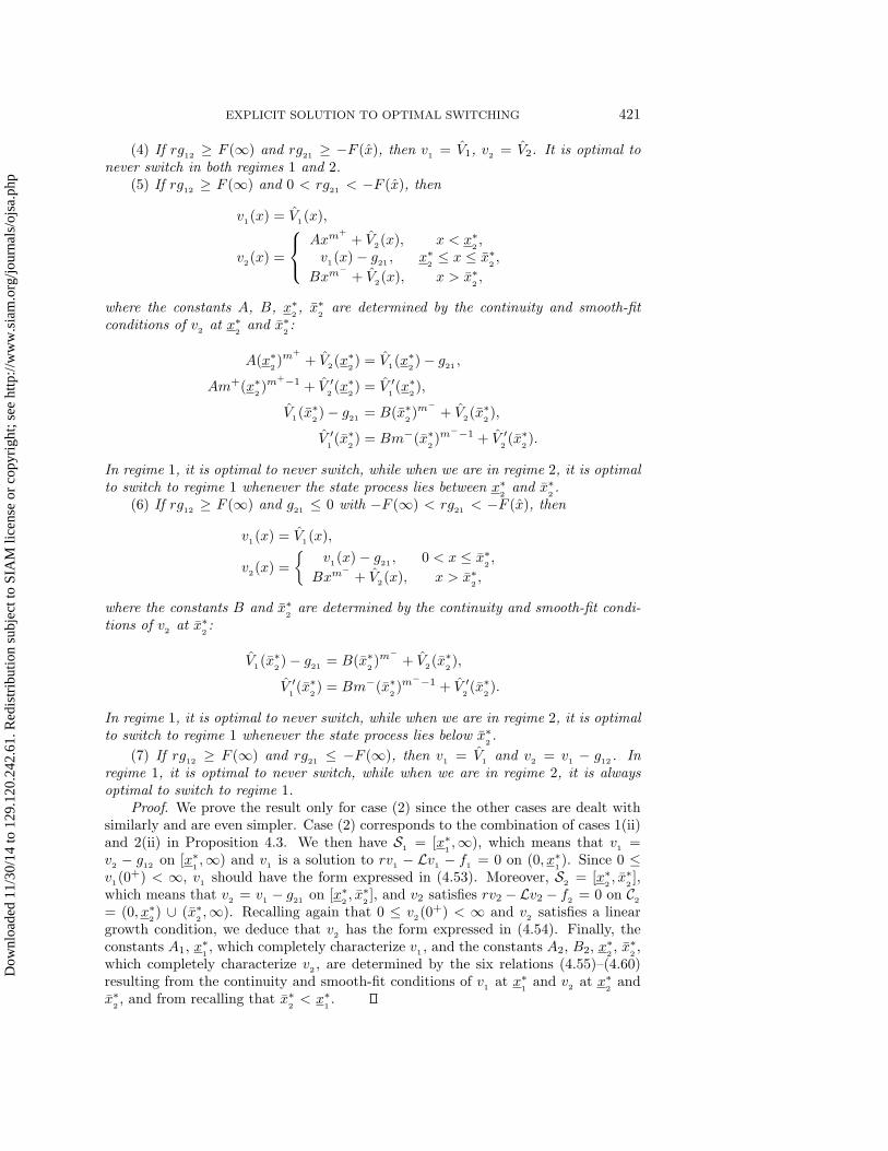
regime 1, it is optimal to never switch, while when we are in regime 2, it is alwaysoptimal to switch to regime 1.

Proof. We prove the result only for case (2) since the other cases are dealt withsimilarly and are even simpler. Case (2) corresponds to the combination of cases 1(ii)and 2(ii) in Proposition 4.3. We then have S

1 = [x∗1,∞), which means that v1 =

v2 − g12 on [x∗

1,∞) and v1 is a solution to rv1 − Lv1 − f1 = 0 on (0, x∗

1). Since 0 ≤

v1(0+) < ∞, v1 should have the form expressed in (4.53). Moreover, S2 = [x∗

2, x∗

2],

which means that v2 = v1 − g21 on [x∗2, x∗

2], and v2 satisfies rv2 −Lv2 − f2 = 0 on C2

= (0, x∗2) ∪ (x∗

2,∞). Recalling again that 0 ≤ v

2(0+) < ∞ and v

2satisfies a linear

growth condition, we deduce that v2

has the form expressed in (4.54). Finally, theconstants A1, x

∗1, which completely characterize v1 , and the constants A2, B2, x

∗2, x∗

2,

which completely characterize v2 , are determined by the six relations (4.55)–(4.60)resulting from the continuity and smooth-fit conditions of v1 at x∗

1and v2 at x∗

2and

x∗2, and from recalling that x∗

2< x∗

1.

Dow

nloa

ded

11/3

0/14

to 1

29.1

20.2

42.6

1. R

edis

trib

utio

n su

bjec

t to

SIA

M li

cens

e or

cop

yrig

ht; s

ee h

ttp://

ww

w.s

iam

.org

/jour

nals

/ojs

a.ph

p


Remark 4.3. In the classical approach, for instance in case (2), we construct apriori a candidate solution in the form (4.53)–(4.54) and we have to check the existenceof a sextuple solution to (4.55)–(4.60), which may be somewhat tedious! Here, by theviscosity solutions approach, and since we already state the smooth-fit C1 propertyof the value functions, we know a priori the existence of a sextuple solution to (4.55)–(4.60).

Appendix A. Proof of comparison principle. In this section, we prove acomparison principle for the system of variational inequalities (3.8). The comparisonresult in [10] for switching problems in a finite horizon does not apply in our context.Inspired by [8], we first produce some suitable perturbation of a viscosity supersolutionto deal with the switching obstacle, and then follow the general viscosity solutiontechnique; see, e.g., [3].

Theorem A.1. Suppose ui, i ∈ Id, are continuous viscosity subsolutions tothe system of variational inequalities (3.8) on (0,∞), and wi, i ∈ Id, are continu-ous viscosity supersolutions to the system of variational inequalities (3.8) on (0,∞),satisfying the boundary conditions ui(0

+) ≤ wi(0+), i ∈ Id, and the linear growth

condition

|ui(x)| + |wi(x)| ≤ C1 + C2x ∀x ∈ (0,∞), i ∈ Id,(A.1)

for some positive constants C1 and C2. Then,

ui ≤ wi on (0,∞) ∀i ∈ Id.

Proof. Step 1. Let ui and wi, i ∈ Id, as in Theorem A.1. We first construct strictsupersolutions to the system (3.8) with suitable perturbations of wi, i ∈ Id. We set

h(x) = C ′1 + C ′

2xp, x > 0,

where C ′1, C

′2 > 0, and p > 1 are positive constants to be determined later. We then

define for all λ ∈ (0, 1) the continuous functions on (0,∞) by

wλi = (1 − λ)wi + λ(h + αi), i ∈ Id,

where αi = minj �=i gji. We then see that for all λ ∈ (0, 1), i ∈ Id,

wλi − max

j �=i(wλ

j − gij) = λαi + (1 − λ)wi − maxj �=i

[(1 − λ)(wj − gij) + λαj − λgij ]

≥ (1 − λ)[wi − maxj �=i

(wj − gij)] + λ

(αi + min

j �=i(gij − αj)

)

≥ λmini∈Id

(αi + min

j �=i(gij − αj)

)≥ λν,(A.2)

where ν := mini∈Id[αi + minj �=i(gij − αj)] is a constant independent of i. We now

check that ν > 0, i.e., νi := αi +minj �=i(gij −αj) > 0, ∀i ∈ Id. Indeed, fix i ∈ Id, andlet k ∈ Id such that minj �=i(gij − αj) = gik − αk and set i such that αi = minj �=i gji= gii. We then have

νi = gii + gik − minj �=k

gjk > gik − minj �=k

gjk ≥ 0

Dow

nloa

ded

11/3

0/14

to 1

29.1

20.2

42.6

1. R

edis

trib

utio

n su

bjec

t to

SIA

M li

cens

e or

cop

yrig

ht; s

ee h

ttp://

ww

w.s

iam

.org

/jour

nals

/ojs

a.ph

p


by (2.6) and thus ν > 0.By definition of the Fenchel–Legendre function in (2.5), and by setting f(1) =

maxi∈Idfi(1), we have for all i ∈ Id,

fi(x) ≤ f(1) + x ≤ f(1) + 1 + xp ∀x > 0.

Moreover, recalling that r > b := maxi bi, we can choose p > 1 s.t.

ρ := r − pb− 1

2σ2p(p− 1) > 0,

where we set σ := maxi σi > 0. By choosing

C ′1 ≥ 2 + f(1)

r− min

iαi,C

′2 ≥ 1

ρ,

we then have for all i ∈ Id,

rh(x) − Lih(x) − fi(x) = rC ′1 + C ′

2xp

[r − pbi −

1

2σ2i p(p− 1)

]− fi(x)

≥ rC ′1 + ρC ′

2xp − fi(x)

≥ 1 ∀x > 0.(A.3)

From (A.2) and (A.3), we then deduce that for all i ∈ Id, λ ∈ (0, 1), wλi is a superso-

lution to

min

{rwλ

i − Liwλi − fi, w

λi − max

j �=i(wλ

j − gij)

}≥ λδ on (0,∞),(A.4)

where δ = ν ∧ 1 > 0.Step 2. In order to prove the comparison principle, it suffices to show that for all

λ ∈ (0, 1),

maxj∈Id

sup(0,+∞)

(uj − wλj ) ≤ 0

since the required result is obtained by letting λ go to 0. We argue by contradictionand suppose that there exist some λ ∈ (0, 1) and i ∈ Id s.t.

θ := maxj∈Id

sup(0,+∞)

(uj − wλj ) = sup

(0,+∞)

(ui − wλi ) > 0.(A.5)

From the linear growth condition (A.1), and since p > 1, we observe that ui(x)−wλi (x)

goes to −∞ when x goes to infinity. By choosing also C ′1 ≥ maxi wi(0

+), we thenhave ui(0

+)−wλi (0+) = ui(0

+)−wi(0+) + λ(wi(0

+)−C ′1) ≤ 0. Hence, by continuity

of the functions ui and wλi , there exists x0 ∈ (0,∞) s.t.

θ = ui(x0) − wλi (x0).

For any ε > 0, we consider the functions

Φε(x, y) = ui(x) − wλi (y) − φε(x, y),

φε(x, y) =1

4|x− x0|4 +

1

2ε|x− y|2

Dow

nloa

ded

11/3

0/14

to 1

29.1

20.2

42.6

1. R

edis

trib

utio

n su

bjec

t to

SIA

M li

cens

e or

cop

yrig

ht; s

ee h

ttp://

ww

w.s

iam

.org

/jour

nals

/ojs

a.ph

p


for all x, y ∈ (0,∞). By standard arguments in the comparison principle, the functionΦε attains a maximum in (xε, yε) ∈ (0,∞)2, which converges (up to a subsequence)to (x0, x0) when ε goes to zero. Moreover,

limε→0

|xε − yε|2ε

= 0.(A.6)

Applying Theorem 3.2 in [3], we get the existence of Mε, Nε ∈ R such that

(pε,Mε) ∈ J2,+ui(xε),

(qε, Nε) ∈ J2,−wλi (yε),

where

pε = Dxφε(xε, yε) =1

ε(xε − yε) + (xε − x

0)3,

qε = −Dyφε(xε, yε) =1

ε(xε − yε),

and (Mε 00 −Nε

)≤ D2φε(xε, yε) + ε

(D2φε(xε, yε)

)2(A.7)

with

D2φε(xε, yε) =

(3(xε − x

0)2 + 1

ε − 1ε

− 1ε

1ε

).

By writing the viscosity subsolution property (3.9) of ui and the viscosity strict su-persolution property (A.4) of wλ

i , we have the following inequalities:

min

{rui(xε) −

(1

ε(xε − yε) + (xε − x0)

3

)bixε −

1

2σ2i x

2εMε − fi(xε),

ui(xε) − maxj �=i

(uj − gij)(xε)

}≤ 0,(A.8)

min

{rwλ

i (yε) −1

ε(xε − yε)biyε −

1

2σ2i y

2εNε − fi(yε),

wλi (yε) − max

j �=i(wλ

j − gij)(yε)

}≥ λδ.(A.9)

We then distinguish the following two cases:(1) ui(xε) − maxj �=i(uj − gij)(xε) ≤ 0 in (A.8).By sending ε → 0, this implies

ui(x0) − maxj �=i

(uj − gij)(x0) ≤ 0.(A.10)

On the other hand, we have by (A.9):

wλi (yε) − max

j �=i(wλ

j − gij)(yε) ≥ λδ,

Dow

nloa

ded

11/3

0/14

to 1

29.1

20.2

42.6

1. R

edis

trib

utio

n su

bjec

t to

SIA

M li

cens

e or

cop

yrig

ht; s

ee h

ttp://

ww

w.s

iam

.org

/jour

nals

/ojs

a.ph

p


so that by sending ε to zero,

wλi (x0) − max

j �=i(wλ

j − gij)(x0) ≥ λδ.(A.11)

Combining (A.10) and (A.11), we obtain

θ = ui(x0) − wλi (x0) ≤ −λδ + max

j �=i(uj − gij)(x0) − max

j �=i(wλ

j − gij)(x0)

≤ −λδ + maxj �=i

(uj − wλj )(x0)

≤ −λδ + θ,

which is a contradiction.(2) rui(xε) −

(1ε (xε − yε) + (xε − x0)

3)bixε − 1

2σ2i x

2εMε − fi(xε) ≤ 0 in (A.8).

Since by (A.9), we also have

rwλi (yε) −

1

ε(xε − yε)biyε −

1

2σ2i y

2εNε − fi(yε) ≥ λδ,

this yields, by combining the above two inequalities,

rui(xε) − rwλi (yε) −

1

εbi(xε − yε)

2 − (xε − x0)3bixε

+1

2σ2i y

2εNε −

1

2σ2i x

2εMε + fi(yε) − fi(xε) ≤ −λδ.(A.12)

Now, from (A.7), we have

1

2σ2i x

2εMε −

1

2σ2i y

2εNε ≤

3

2εσ2i (xε − yε)

2 +3

2σ2i x

2ε(xε − x0)

2(3ε(xε − x0)

2 + 2),

so that by plugging into (A.12), we have

r(ui(xε) − wλ

i (yε))≤ 1

εbi(xε − yε)

2 + (xε − x0)3bixε +

3

2εσ2i (xε − yε)

2

+3

2σ2i x

2ε(xε − x0)

2(3ε(xε − x0)

2 + 2)

+ fi(yε) − fi(xε) − λδ.

By sending ε to zero, and using (A.6), continuity of fi, we obtain the required con-tradiction that rθ ≤ −λδ < 0. This ends the proof of Theorem A.1.

Acknowledgments. We would like to thank Xin Guo for discussions. We arealso grateful to the anonymous referees for constructive suggestions and commentsthat helped to improve the paper.

REFERENCES

[1] A. Bensoussan and J. L. Lions, Controle impulsionnel et inequations variationnelles, Dunod,Paris, 1982.

[2] K. A. Brekke and B. Øksendal, Optimal switching in an economic activity under uncertainty,SIAM J. Control Optim., 32 (1994), pp. 1021–1036.

[3] M. Crandall, M. H. Ishii, and P. L. Lions, User’s guide to viscosity solutions of secondorder partial differential equations, Bull. Amer. Math. Soc., 27 (1992), pp. 1–67.

[4] A. Dixit and R. Pindick, Investment under uncertainty, Princeton University Press, Prince-ton, NJ, 1994.

Dow

nloa

ded

11/3

0/14

to 1

29.1

20.2

42.6

1. R

edis

trib

utio

n su

bjec

t to

SIA

M li

cens

e or

cop

yrig

ht; s

ee h

ttp://

ww

w.s

iam

.org

/jour

nals

/ojs

a.ph

p


[5] K. Duckworth and M. Zervos, A model for investment decisions with switching costs, Ann.Appl. Probab., 11 (2001), pp. 239–250.

[6] W. H. Fleming and H. M. Soner, Controlled Markov Processes and Viscosity Solutions,Springer-Verlag, New York, 1993.

[7] X. Guo, An explicit solution to an optimal stopping problem with regime switching, J. Appl.Probab., 38 (2001), pp. 464–481.

[8] H. Ishii and P. L. Lions, Viscosity solutions of fully nonlinear second order elliptic partialdifferential equations, J. Differential Equations, 83 (1990), pp. 26–78.

[9] H. Pham, On the smooth-fit property for one-dimensional optimal switching problem, inSeminaire de Probabilites, Vol. XL, to appear.

[10] S. Tang and J. Yong, Finite horizon stochastic optimal switching and impulse controls witha viscosity solution approach, Stoch. Stoch. Rep., 45 (1993), pp. 145–176.

Dow

nloa

ded

11/3

0/14

to 1

29.1

20.2

42.6

1. R

edis

trib

utio

n su

bjec

t to

SIA

M li

cens

e or

cop

yrig

ht; s

ee h

ttp://

ww

w.s

iam

.org

/jour

nals

/ojs

a.ph

p

explicit solution to an optimal switching problem in the two‐regime case

Documents