dynamic portfolio optimization with a defaultable … · dynamic portfolio optimization with a...

Introduction The Model Portfolio Optimization Verification Theorems Logarithmic Utility Conclusions

Dynamic Portfolio Optimization with a DefaultableSecurity and Regime Switching

Jose E. Figueroa-Lopez

Department of StatisticsPurdue University

[email protected]

INFORMSCredit and Counterparty Risk

November 14, 2011(joint work with Agostino Capponi)


Regime Switching Models and Portfolio Optimization

1 Why regime switching? Market and credit factors exhibitdifferent behavior depending on the overall state of economy,as measure by, e.g., a macro-economic index Ct .

2 Portfolio Optimization focused on default-free markets:Guo et al. (2005); Nagai & Runggaldier (2008); Sotomayor &Cadenillas (2009);

3 Defaultable bonds are a significant portion of the market.4 Portfolio optimization problems with defaultable securities has

focused on Brownian driven risky factors:

Bielecki & Jang (2006), Bo et al. (2010), Lakner & Liang(2008), Jeanblanc & Runggaldier (2010);

5 Our goal:Develop a framework for solving finite horizon portfoliooptimization problems under regime switching markets with adefaultable bond.





3 Defaultable bonds are a significant portion of the market.

4 Portfolio optimization problems with defaultable securities hasfocused on Brownian driven risky factors:







3 Defaultable bonds are a significant portion of the market.4 Portfolio optimization problems with defaultable securities has

focused on Brownian driven risky factors:




Overview of Main Results

Considered Merton’s utility maximization problem from wealth(without consumption) in finite-horizon with a risk-free(default-free) asset, a risky asset, and a defaultable bondunder Markov driven regime switching;

Established the Hamilton-Jacobi-Bellman (HJB) Equations forthe optimal value function of the problem;

Proved Verification Theorems for the HJB equations;

Found closed form representations for the logarithm utilityU(v) = log v in terms of the solution of a system of first orderlinear ODE;

Determined conditions for the “directionality” (short or long)of the optimal trading strategies for the defaultable bond;


Regime Switching Market Model

The states of the economy are modeled by a continuous-timeMarkov process {Ct};The process {Ct} has finite state space {1, 2, . . . ,N} andgenerator A(t) = [Ai ,j(t)]i ,j=1,...,N :

Ai ,j(t) = limh→0

1

h{P(Ct+h = j |Ct = i)− δi ,j} ;

Money market account:For predefined potential rate values (r1, . . . , rN) ∈ RN ,

dBt = r(t)Btdt, r(t) = rCt

;

Risky asset:For predefined potential (µ1, . . . , µN) and (σ1, . . . , σN),

dSt = µ(t)Stdt + σ(t)StdWt , S0 = s,

µ(t) = µCt, σ(t) := σ

Ct, W⊥C .


Default Model

1 The default time τ is defined in terms of a given hazardprocess {h(t)}t≥0, driven by state of the economy:

h(t) := hCt, for some predefined (h1, . . . , hN).

2 We adopt the double-stochastic framework to default where

τ := inf{t ∈ R+ :

∫ t

0h(u)du ≥ χ

},

for χ ∼ exp(1) indep. of X and W .3 Notation:

Ft : flow of information of the whole market, excluding default;Ht : flow of information generated by the default processHt = 1t≥τ ;G = (Gt) = Ft ∨Ht : flow of information, including default;


Defaultable Bond

Given a recovery process (zt)t , the bond price is defined by

p(t,T ) = EQ[e−

R τt rsds zτ1{t<τ≤T} + e−

R Tt rsds1{τ≥T}

∣∣∣Gt

],

for a suitable risk-neutral pricing measure Q;Under Q, W is still a Wiener process and C is still a Markovprocesses indep. of W , but with generator AQ(t) = [aQ

i ,j(t)];Assume the recovery-of-market value scheme:zt := (1− L(t))p(t−,T ). Hence,

p(t,T ) = 1{τ>t}EQ[e−

R Tt [r(s)+h(s)L(s)]ds

∣∣∣∣Ft

].

We assume that L(t) = LCt

with some given (L1, . . . , LN).Notation:

ψi (t) := EQ[e−


∣∣∣∣Ct = i

].


Defaultable Bond


p(t,T ) = EQ[e−


R Tt rsds1{τ≥T}

∣∣∣Gt

],

for a suitable risk-neutral pricing measure Q;

Under Q, W is still a Wiener process and C is still a Markovprocesses indep. of W , but with generator AQ(t) = [aQ


p(t,T ) = 1{τ>t}EQ[e−


∣∣∣∣Ft

].



ψi (t) := EQ[e−


∣∣∣∣Ct = i

].


Defaultable Bond


p(t,T ) = EQ[e−


R Tt rsds1{τ≥T}

∣∣∣Gt

],


i ,j(t)];

Assume the recovery-of-market value scheme:zt := (1− L(t))p(t−,T ). Hence,

p(t,T ) = 1{τ>t}EQ[e−


∣∣∣∣Ft

].



ψi (t) := EQ[e−


∣∣∣∣Ct = i

].


Defaultable Bond


p(t,T ) = EQ[e−


R Tt rsds1{τ≥T}

∣∣∣Gt

],



p(t,T ) = 1{τ>t}EQ[e−


∣∣∣∣Ft

].


with some given (L1, . . . , LN).

Notation:

ψi (t) := EQ[e−


∣∣∣∣Ct = i

].


Defaultable Bond


p(t,T ) = EQ[e−


R Tt rsds1{τ≥T}

∣∣∣Gt

],



p(t,T ) = 1{τ>t}EQ[e−


∣∣∣∣Ft

].



ψi (t) := EQ[e−


∣∣∣∣Ct = i

].


Problem Setup

Assumptions

Investor wants to maximize her expected final utility fromwealth, EP(U(VR)), at a finite horizon R ≤ T ;

Investor can dynamically allocate her financial wealth into therisk-free bank account, the stock, and the defaultable T -bond.

Investor does not have intermediate consumption nor capitalincome to support purchase of assets (self-financiability).


Problem Setup

The Wealth Dynamics

Let πu := (πBu , π

Su , π

Pu ) represent fractions of wealth invested

in bank account, stock, and defaultable bond at time u.

The dynamics of the wealth process V πu := V π,t,v

u is

dV πu = V π

u−

{πB

u

dBu

Bu+ πS

u

dSu

Su+ πP

u

dp(u,T )

p(u−,T )

}, u ≥ t,

V π,t,vt = v

where πB + πP + πS = 1


The Utility Maximization Problem

The Optimization Problem

Dynamic Optimization Problem with horizon R ≤ T

ϕR(t, v , i , z) := supπ∈At(v ,i ,z)

EP[U(V π,t,v

R )

∣∣∣∣Vt = v ,Ct = i ,Ht = z

]for each (v , i , z) ∈ (0,∞)× {1, 2, . . . ,N} × {0, 1}, a given utilityfunction U : [0,∞)→ R ∪ {∞}, and a suitable class of Feedbackor Markov admissible strategies At(v , i , z).


HJB formulation

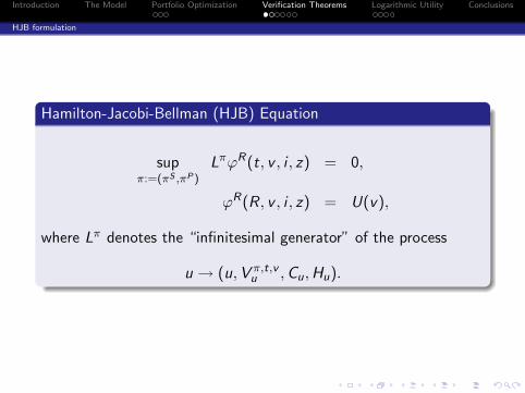
Hamilton-Jacobi-Bellman (HJB) Equation

supπ:=(πS ,πP)

LπϕR(t, v , i , z) = 0,

ϕR(R, v , i , z) = U(v),

where Lπ denotes the “infinitesimal generator” of the process

u → (u,V π,t,vu ,Cu,Hu).


HJB formulation

HJB Equation

Let ϕi ,z(t, v) := ϕR(t, v , i , z) denote the value function. Then

Lϕi ,z(t, v) = 0

ϕi ,z(R, v) = U(v)

where

Lϕi,z (t, v) :=∂ϕi,z

∂t+ vri

∂ϕi,z

∂v+ z

Xj 6=i

ai,j (t)ˆϕj,z (t, v)− ϕi,z (t, v)

˜+ max

πSi

(πS

i (µi − ri )v∂ϕi,z

∂v+ (πS

i )2 σ2i

2v2 ∂

2ϕi,z

∂v2

)

+ (1− z) maxπP

i

πP

i θi (t)v∂ϕi,z

∂v+ hi

hϕi,1(t, v(1− πP

i ))− ϕi,z (t, v)i

+Xj 6=i

ai,j (t)

»ϕj,z

„t, v

»1 + πP

i

„ψj (t)

ψi (t)− 1

«–«− ϕi,z (t, v)

–ff

with θi = hiLi −∑

j 6=i aQi ,j(t)

ψj (t)ψi (t) − aQ

i ,i (t).


Post-Default case

Notation

ηi := µi−riσi

denotes the sharpe ratio of the stock under the i th

economic regime;

S1,2 denotes the class of functions$ : [0,R]× R+ × {1, . . . ,N} → R+ such that

$(·, ·, i) ∈ C 1,2((0,R)× R+) ∩ C ([0,R]× R+)

$v (s, v , i) ≥ 0, $vv (s, v , i) ≤ 0

for each i = 1, . . . ,N.


Post-Default case

Post-Default Verification Theorem

Capponi & F-L (2011)

Suppose there exists a function w ∈ S1,2 that solve the nonlinearDirichlet problem

wt(s, v , i) + rivwv (s, v , i) +Xj 6=i

ai,j (s) (w(s, v , j)− w(s, v , i))−η2

i

2

w2v (s, v , i)

wvv (s, v , i)= 0,

with terminal condition w(R, v , i) = U(v). Then,

w is the optimal post-default value function ϕR(t, v , i , 1);

The optimal fraction of wealth investment in the stock underthe i th economic regime is

π∗iS (s, v) = −

ηi

σi

wv (s, v , i)

vwvv (s, v , i),

at time s when the wealth is v .


Pre-Default Case

Pre-Default Verification Theorem

Assumptions

Assume that w ∈ S1,2 and pi = pi (s, v), i = 1, . . . ,N, solvesimultaneously the following system of equations:

θi (s)w v (s, v , i)− hi ϕRv (s, v(1− pi ), i)

+∑j 6=i

ai,j(s)(ψj (s)ψi (s) − 1

)w v

(s, v

[1 + pi

(ψj (s)ψi (s) − 1

)], j)

= 0,

w t(s, v , i)− η2i

2w2

v (s,v ,i)w vv (s,v ,i) + rivw v (s, v , i)

+

{piθi (t)vw v (s, v , i) + hi

[ϕR(s, v(1− pi ), i)− w(s, v , i)

]+∑j 6=i

ai,j(t)[w(s, v

(1 + pi

(ψj (s)ψi (s) − 1

)), j)− w(s, v , i)

]}= 0,

for t < s < R, with terminal condition w(R, v , i) = U(v).


Pre-Default Case

Pre-Default Verification Theorem

Statements. Capponi & F-L (2011)

(1) w(t, v , i) is the optimal pre-default value function

ϕR(t, v , i) = ϕR(t, v , i , 0),

(2) The optimal percentage of wealth invested in the stock andthe defaultable bond under the i th economic regime is

π∗iS(s, v , z) = −ηi

σi

w v (s, v , i)

vw vv (s, v , i)(1− z)− ηi

σi

wv (s, v , i)

vwvv (s, v , i)z ,

π∗iP(s, v , z) = pi (s, v)(1− z),

at time s when the wealth process v and the default state is z .


Optimal Strategies for U(v) = log(v)

Proposition (Capponi & F-L, 2011)

(1) The optimal fraction of wealth invested in the stock under thei th economic regime:

π∗iS =

µi − riσ2

i

.

(2) The optimal fraction of wealth π∗iP invested in the defaultable

bond under the i th regime is given by the unique solution pi

to system

θi (s)− hi

1− pi+∑j 6=i

ai ,j(s)ψj(s)− ψi (s)

ψi (s) + pi (ψj(s)− ψi (s))= 0.


Optimal Value Functions

Theorem (Capponi & F-L, 2011)

(1) The optimal post-default value function is of the formϕR(t, v , i) = log(v) + K(t, i), where K(t) = (K(t, 1), . . . ,K(t,N)) is theunique positive solution of

Kt(t, i) + ri +η2

i2

+Xj 6=i

ai,j(t)K(t, j) + ai,i (t)K(t, i) = 0,

K(R, i) = 0;

(2) The optimal pre-default value function is of the formϕR(t, v , i) = log(v) + J(t, i), where J(t) = (J(t, 1), . . . , J(t,N)) is theunique positive solution of

Jt(t, i) + ri +η2

i

2+ pi (t)θi (t) + hi (log(1− pi (t)) + K(t, i)− J(t, i))+X

j 6=i

ai,j(t)hlog“1 + pi (t)

“ψj (t)

ψi (t)− 1””

+ J(t, j)− J(t, i)i

= 0,

J(R, i) = 0.


Numerical example

Test scenario

Measure impact of default parameters over value functionsand optimal bond strategies

Focus on a two-regime switching model with time-invariantMarkov chain:

a12 = aQ12 = 0.4, a21 = aQ

21 = 0.1.

Horizon R equal to 3 years.

Regime ‘1’ Regime ‘2’

L 0.4 0.45

r 0.03 0.03

µ 0.07 0.02

σ 0.2 0.2

Table: Parameters associated to the two regimes.


Numerical example

Bond Strategy vs. Time (hQ1 = 0.1)

0 0.5 1 1.5 2 2.5 3−1.4

−1.2

−1

−0.8

−0.6

−0.4

−0.2

0

Horizon R

π 1P(0

)

h2=2

h2=4

h2=6

h2=8

0 0.5 1 1.5 2 2.5 3

0.4

0.5

0.6

0.7

0.8

0.9

1

Horizon R

ψ1(0

)

h2=2

h2=4

h2=6

h2=8

0 0.5 1 1.5 2 2.5 3−1.4

−1.2

−1

−0.8

−0.6

−0.4

−0.2

0

Horizon R

π 2P(0

)

h2=2

h2=4

h2=6

h2=8

0 0.5 1 1.5 2 2.5 30

0.1

0.2

0.3

0.4

0.5

0.6

0.7

0.8

0.9

1

Horizon R

ψ2(0

)

h2=2

h2=4

h2=6

h2=8

Shorted bond units decrease as investment horizon increases.

The riskier the bond, the smaller the number of units you short.

You short more if you are in the riskiest regime.


Numerical example

Post-Default Value Functions

0 0.5 1 1.5 2 2.5 30

0.02

0.04

0.06

0.08

0.1

0.12

0.14

0.16

t

Pos

t−D

efau

lt V

alue

Fun

ctio

n

K(t,1)Merton

0 0.5 1 1.5 2 2.5 30

0.01

0.02

0.03

0.04

0.05

0.06

0.07

0.08

0.09

0.1

t

Pos

t−D

efau

lt V

alue

Fun

ctio

nBoth post-default value functions, K (t, 1) and K (t, 2), arepositive and time decreasing.

They differ at times t far from the investment horizon R andconverge to each other and to Merton for short times tohorizon.


Numerical example

Pre-Default Value Functions (hQ1 = 0.1, LQ

1 = 0.5)

0 0.5 1 1.5 2 2.5 30

0.05

0.1

0.15

0.2

0.25

t

J(t,1

)

h2=2, L2=0.3

h2=4, L2=0.35

h2=6, L2=0.4

h2=8, L2=0.45

0 0.5 1 1.5 2 2.5 30

0.05

0.1

0.15

0.2

0.25

0.3

0.35

tJ(

t,2)

h2=2, L2=0.3

h2=4, L2=0.35

h2=6, L2=0.4

h2=8, L2=0.45

Both pre-default value functions, J(t, 1) and J(t, 2) arepositive and time decreasing

As default risk increases, pre-default approaches post-defaultvalue function


Conclusions

Develop a framework for solving continuous time portfoliooptimization problems in regime switching defaultablemarkets, consisting of risky asset, defaultable security andrisk-free asset.

Proved verification theorems for pre-default and post-defaultutility maximization subproblems.

Demonstrated our framework on a logarithmic utility investor

dynamic portfolio optimization with a defaultable … · dynamic portfolio optimization with a...

Documents