Defaultable Security Valuation and Model Risk

Aydin Akgun1,2

This Version: March 2001

1HEC, University of Lausanne, and FAME (International Center for Financial AssetManagement and Engineering), Geneva, Switzerland. I would like to thank my thesis su-pervisor Prof. Rajna Gibson (ISB, University of Zurich) for her continual support through-out the study. The financial support of RiskLab (Zurich) is gratefully acknowledged. Allcomments are welcome.

2Address: Swiss Banking Institute, University of Zurich, Plattenstrasse 14, 8032 Zurich,Switzerland. Tel: ++41-1-6342782, Email: akgun@isb.unizh.ch

Abstract

The aim of the paper is to analyse the effects of different model specifications, withina general nested framework, on the valuation of defaultable bonds, and some creditderivatives. Assuming that the primitive variables such as the risk-free short rate,and the credit spread are affine functions of a set of state variables following jump-diffusion processes, efficient numerical solutions for the prices of several defaultablesecurities are provided. The framework is flexible enough to permit some degree offreedom in specifying the interrelation among the primitive variables. It also allows aricher economic interpretation for the default process. The model is calibrated, anda sensitivity analysis is conducted with respect to parameters defining jump terms,and correlation. The effectiveness of dynamic hedging strategies are analysed as well.

JEL Codes: G13, G19

1 Introduction

The aim of this paper is to analyse model risk within the context of credit risk mod-eling, and more specifically for defaultable bonds and credit derivatives. With theproliferation of financial losses related to the use of derivative securities risk man-agement in general, and model risk management in particular has gained attentionin the recent years. Recently, the booming credit risk literature has experienced ashift towards the so called reduced-form models that rely, basically, on an exogenousspecification of default-inducing processes. The reason is that these models are moreamenable to empirical testing and, given suitable assumptions on recovery rates, al-low straightforward application of the already available martingale pricing technology.In this vein, it is also easier to analyse market risk and credit risk together, whichis crucial for versatile financial institutions operating in dynamic and intertwinedenvironments.The paper contributes to the credit risk literature in several ways. First, de-

faultable securities are priced in a framework that is unprecedented in its generality.Second, an extensive analysis of the effects, on valuation, of jump terms in bothriskless interest rates and credit spreads is provided. Third, the influence of corre-lation between riskless interest rates and credit spreads is also analysed both fromvaluation, and hedging perspectives. Although jumps in interest rates recently havereceived some attention (see Akgun (2000) and references therein), the presence ofjumps in credit spread dynamics has been so far ignored in both the empirical andtheoretical literature.1 As the distributions implied by observed credit spread dy-namics are highly leptokurtic the relevance of incorporating jumps into the analysisbecomes clear. There has also been a relatively higher but mostly qualitative interestin the correlation between market and credit risks, especially from a risk measure-ment perspective. The analysis in this paper, specifically sets out to quantify theeffects of this correlation in pricing and hedging several defaultable securities. Theframework of the paper is basically as follows. There are three state variables follow-ing jump-diffusion processes. The diffusion part is of CIR (1985) type. The risklessshort-rate and the credit spread are affine functions of the state variables. There arethree types of jumps. Jumps unique to the interest rate, jumps pertaining to thecredit spread, and jumps common to both processes with a joint jump-size distribu-tion depending only on time. The diffusion part formulation is such that negativecorrelation between credit spreads and interest rates is allowed, and positivity of thespread is guaranteed. The positivity is no longer guaranteed when one takes intoaccount the normally distributed jump sizes. Empirically, however, it turns out thatnegative state variables are possible only with a very small probability. The modelalso is admissible in the sense of Dai and Singleton (1999). Volatilities, drifts, andintensities can be stochastic provided they are affine in state variables. Such a frame-work permits one to distinguish the effects of economy-wide shocks from firm-specific

1The empirical evidence for jumps in the dynamics of credit spreads is not lacking. LTCM isbelieved to have lost more than $500 million because of a jump of nearly %17 in credit spreads.Such jumps become especially important when the correlation structure of state variables defininginterest rate and credit risks is substantially altered during financial market turmoil.

1

ones, as well as being open to other interpretations for the jump terms. More impor-tantly, one can see the effects of the interaction between market risk and credit risk.Tractable solutions of this model are possible using the affine-pricing methodologydeveloped by Duffie, Pan, and Singleton (1999), and Bakshi and Madan (1999) whichinvolves decomposing an option-like payoff into principal securities, and valuing eachof these through the Fourier inversion of its characteristic function. Model parameterscan be estimated in two steps as in Duffee (1999) if one assumes away the commonjump term. This is essential for estimation since simultaneous use of the treasurybond data and corporate bond data to estimate the whole set of parameters wouldbe cumbersome and highly impecise.Given this setup, the aim is to analyse the effects, on pricing, of different specifi-

cations regarding the jump terms and the correlation between the riskless short-rateand the credit spread. The securities that will be priced, as examples, are a de-faultable bond, a put option on the defaultable bond, a credit spread option, anda call option on the credit spread. Analysing these credit derivatives with differentpayoff structures will allow a better assessment of the relation between market riskand credit risk, and differential impact of jump terms. In this regard, conductingsensitivity analysis with respect to relevant parameters may provide further insights.The efficiency of modelisation can also be tested in this nested framework, in termsof pricing. It is at this point that an analysis from the perspective of model misspeci-fication becomes relevant. Aside from pricing issues, improvements gained with morerealistic assumptions in the partial hedging of defaultable securities can be comparedto those of simpler models. Before closing this section, note that any attempt toquantify model risk is dependent on a chosen benchmark model. The benchmarkmodel is implicitly assumed to be closer to reality, and the performance, in an ap-propriately defined sense, of any submodel that is inferior to it can be evaluated andquantified with respect to the benchmark model. Such an analysis is especially ofimportance from the viewpoint of an economic agent trying to select or evaluate amodel to use in pricing, trading, or hedging derivative securities.Before explaining the theoretical framework it may be illustrative to briefly touch

upon the related literature which would also allow a better comparison with thepresent article. There are two, quite distinct, brands of research focusing on thepricing of credit risk. These are named as structural, and reduced-form approaches.The structural approach represents and encompasses various extensions of Merton(1974)’s work on the pricing of corporate debt. In this brand of the literature defaultoccurs when the firm asset value process hits a lower boundary that can be prede-termined and fixed (for instance the face value of debt) or endogeneously determinedas the outcome of bargaining between shareholders and creditors. The problem withsuch models is that to be realistic they need to specify, rather elaborately, the condi-tions triggering default and the capital structure of the firm in question. Even with acomplex specification, however, the empirical performance of these models have beendisappointing. Moreover, by their very nature (since default stopping time is not in-accessible), they sharply underestimate credit spreads for short time horizons. Theseand other considerations led researchers to model the default event exogeneously,as the first jump of a Cox process with certain intensity for instance. Jarrow and

2

Turnbull (1995) article is one of the precursors in this area. In their model defaulttime is exponentially distributed, with constant intensity and the default process isindependent of the riskless interest rate. Their approach involves building trees forthe riskless term structure and the default process, and inferring risk-neutral defaultprobabilities from the observed market prices of corporate bonds. This model hasbeen later extended to the case where default time follows a continuous-time discretestate Markov chain to allow valuation of derivatives based on credit ratings. (See Jar-row, Turnbull, and Lando (1997), and Lando (1998). There has also been attemptsto recast the HJM (1992) framework to take into account default risk by modeling de-faultable forward rates directly and then derive the restrictions necessary to rule outarbitrage. Das and Tufano (1995), and Schonbucher (1998) can be cited as examples.Yet another subgroup of research within reduced-form models have been initiated byDuffie and Singleton (1999). Assuming that recovery value, upon default, is propor-tional to the market value an instant before default they showed that the ordinarymartingale valuation methodology can still be used to value defaultable bonds byadding an adjustment term to the riskless discount rate. The present paper departsfrom these and other previous research in several ways. First, it represents the firstattempt to model credit spreads as jump-diffusions. Second, as explained above theproposed model is very general in other aspects as well. Third, in the empirical partaccompanying the theoretical pricing framework an extensive sensitivity analysis isconducted from a model risk perspective.The paper proceeds as follows: First, the reduced form approach is outlined briefly.

In the next section the theoretical framework is laid out in its full generality, andtransform analysis, and credit derivative valuation are explained. Section 3 deals withthe particular model proposed along with subsections on data and implementationissues, hedging considerations, and the details of the numerical integration techniquesemployed. In Section 4 results are presented and interpreted from a model riskperspective. Section 5 concludes with a discussion assessing the relevance of thefindings for pricing credit sensitive securities, and for risk management.

1.1 The Reduced Form Approach

In this subsection, we briefly present the valuation formula resulting from the workof Duffie and Singleton (1999). This formula will be the essential pricing ingredientfor a large part of this paper. Assume that markets are perfect and an equivalentmartingale measure exists. Consider a defaultable claim with a random promisedpayoff of H at maturity T . When default occurs at time T d, it is unpredictable, andit involves a loss rate of L(T d) in the market value of the claim. Hence, the value attime t of this claim can be written, under the risk neutral measure, as

St = Et

exp−TΛTdZ

t

rsds

hHIT<Td + S(T d) ¡1− L(T d)¢ IT≥Tdi (1)

Duffie and Singleton (1999) showed that (1) is, under mild conditions2, equivalent to

3

St = Et

exp− TZ

t

Rsds

H (2)

with Rt = rt + htLt where ht denotes the hazard rate of the default process. (2)

means that we can value a defaultable claim as if its payoff is riskless, but discountedat a default-adjusted discount rate, given above by Rt. In this paper we are goingto denote default adjustment term htLt by st and call it somewhat informally asthe credit spread. Note that the same approach can be used to value coupon bondsas well. Apart from allowing straightforward discounting of payoffs of defaultableclaims, the proportional loss in market value assumption helps preserve the simplevalue additivity rule for coupon bonds. (Jarrow and Turnbull (2000))

2 The Theoretical Framework

We operate in the context of a perfect continuous-time economy with a trading in-terval [0, T ∗], T ∗ being kept fixed. Uncertainty in capital markets is characterisedthrough a probability space (Ω,=,z, P ), with z = =(t) : t ∈ [0, T ∗] denoting theP−completed, right-continuous filtration generated by a set of state variables follow-ing jump-diffusion processes. r is the instantaneous riskless interest rate which isequivalently called as the riskless short rate in this paper. The price at time t of ariskless zero-coupon (defaultable) bond maturing at T (for 0 < T ≤ T ∗) is denoted byB(t, T ) (Bd(t, T )). The existence of an equivalent martingale measure is assumed, andin the following all expectations are taken with respect to this measure unless notedotherwise.3 The state variables in the economy are denoted by an n-dimensionalstrong Markov process uniquely solving the following SDE :

Xt = X0 +

tZ0

µ(Xs, s)ds+

tZ0

σ(Xs, s)dW (s) +

tZ0

J(s)dN(s) (3)

where W is a d-dimensional independent standard Brownian motion, N is a vector

Poisson process of intensity λ(Xt, t), with a random jump-size matrix J(t) whosedistribution depends only on time t, and µ and σ are conformable coefficients thatare affine in the state variables. For additional technical details see Duffie, Pan, andSingleton (1999). The risk-free short rate, and credit spread are also assumed to beaffine in the state variables. That is,

2An important condition is that jumps in the conditional distribution of S, h, or L occur withprobability zero at the default time T d.

3The particular choice of the equivalent martingale measure is implicitly left to the market, orto the representative agent, if any. This wave-off is typical in this brand of asset pricing literature.

4

µ(x, t) = µ0(t) + µ1(t) · x (4)

σ(x, t)σT (x, t) = σ0(t) + σ1(t) · x (5)

λ(x, t) = λ0(t) + λ1(t) · x (6)

r(x, t) = r0(t) + r1(t) · x (7)

s(x, t) = s0(t) + s1(t) · x (8)

2.1 Transform Analysis and Affine Pricing

In this subsection we use the so called transform analysis methodology to value de-faultable bonds and some specific credit derivatives. This methodology has beenknown, in less general terms, in the finance literature since 1980s and has been sinceimproved and formalized by Bakshi and Madan (2000), and by Duffie, Pan, andSingleton (1999). These authors used the technique to value certain options, andDuffie, Pan, and Singleton (1999) also stated that it could be used to value default-able bonds as well. However, none of these papers addressed the issue of credit riskpricing explicitly.To begin with, define two related objects as follows

Ψrt,T ; a,b(Xt, a0, b0) = Et

exp− TZ

t

r(Xs, s)ds

(a+ b ·XT )ea0+b0·XT (9)

and

ΨRt,T ; a,b(Xt, a0, b0) = Et

exp− TZ

t

R(Xs, s)ds

(a+ b ·XT )ea0+b0·XT (10)

where r is the riskless short rate and R is the risk-adjusted discount rate. Notethat Ψrt,T ; 1,0(Xt, 0,0) gives the value at time t of a riskless zero-coupon bond pay-ing $1 at maturity T . Similarly, ΨRt,T ; 1,0(Xt, 0,0) gives the value of a defaultablebond, assuming, of course, that the assumptions of Section 1.1 hold. The generalizedFeynman-Kac theorem (presented in the Appendix) then implies that

DΨdt,T ; a,b(x, a0, b0)− d(x, t)Ψdt,T ; a,b(x, a0, b0) = 0

with ΨdT,T ; a,b(x, a0, b0) = (a+ b · x)ea0+b0·x (11)

where d is equal to r or R depending on the context and where the infinitesimal

generator D has the form

5

DdΨt,T ; a,b(x, a0, b0) =

∂

∂tΨd(.)(.) +

∂

∂xΨd(.)(.)µ(x, t) +

1

2tr

·∂2

∂x2Ψd(.)(.)σ(x, t)σ

T (x, t)

¸+

LXj=1

λj(x, t)

ZΩ

£Ψd(.)(x+ J

j, .)−Ψd(.)(x, .)¤dF jJ(t) (12)

where F jJ denotes the distribution function of the jump size for the jth jump type.

J j denotes the jth column of the matrix J. In this expression we have denoted thenon-informative arguments of Ψ by a dot to reduce notational burden. To solve (11),we first conjecture in our affine economy that

Ψdt,T ; a=1,b=0(x, a0, b0) = exp [α0(t) + β 0(t) · x] (13)

where the coefficients satisfy the following ODEs:

∂

∂tα0(t) = d0(t)− β 0(t) · µ0(t)− 1

2β 0(t)σ0(t)β 0T (t)

+LXj=1

λj0(t)

1− ZΩ

eβ0(t)·Jj(t)dF jJ(t)

with α0(T ) = a0. (14)

∂

∂tβ0(m)(t) = d(m)1 (t)− β 0(t)µ(m)1 (t)− 1

2β 0(t)σ(m)1 (t)β0T (t)

+LXj=1

λj,(m)1 (t)

1− ZΩ

eβ0(t)·Jj(t)dF jJ(t)

with β0(T ) = b0. (15)

Above again di(t) = ri(t) or ri(t) + si(t) for i = 0, 1 depending on whether we are

interested in Ψr or ΨR. Superscript m in parentheses denotes the mth element of thecorresponding vector. For a matrix, it denotes the mth column. For the tensor σ1 itdenotes the corresponding matrix. Then it can be shown that (see the Appendix)

Ψdt,T ; a,b(x, a0, b0) = Ψdt,T ; a=1,b=0(x, a

0, b0) [α(t) + β(t) · x] (16)

6

with the coefficients satisfying the following ODEs:

− ∂∂tα(t) = β(t) · µ0(t) + β0(t)σ0(t)βT (t)

+LXj=1

λj0(t)

ZΩ

eβ0(t)·Jj(t)(β(t) · J j(t))dF jJ(t)

with α(T ) = a. (17)

− ∂∂tβ(m)(t) = β(t)µ

(m)1 (t) + β0(t)σ(m)1 (t)βT (t)

+LXj=1

λj,(m)1 (t)

ZΩ

eβ0(t)·Jj(t)(β(t) · J j(t))dF jJ(t)

with β(T ) = b. (18)

Hence, the assumed affine structure allows us to value rather complex payoffs de-pending on state variables. The value of such payoffs are completely determined bythe solution of a set of Riccati equations. In some cases closed-form solutions can befound. A substantial literature exists for the numerical solution of Riccati equations,hence one can obtain accurate results with fairly standard procedures, assuming thata solution to the given set of equations exists.

2.2 Valuation of Credit Derivatives

The methodology described above can be extended to value certain derivatives andvulnerable (defaultable) options. A put option on the defaultable bond, for instance,has at the maturity of the option, U < T, the contingent payoff, (K − eα0(U)+β0(U)·x)+whose discounted expectation gives the price of the option. The parameters α0(U)and β 0(U) are found by backward integration (from time T to U) of the set of Riccatiequations defining ΨR. A version of a credit spread option has the payoff (EB(U, T )−Bd(U, T ))+ where B(U, T ) is the price of the riskless bond at the maturity of theoption, Bd(U, T ) is the price of the defaultable bond, and E is a fixed number denotingthe exchange ratio between riskless and defaultable bonds. Since the price of theriskless bond can also be expressed as an exponential affine function of the statevariables, for instance as eα

00(U)+β00(U)·x, it follows that such payoffs can be treated ifwe can evaluate expressions of the following form:

Gt(c, d, y) = Et

exp− UZ

t

r(Xs, s)ds

ec·XU Id·XU ≤ y

(19)

One can easily note that the price at time t of the put option on the defaultable bond

can be expressed as

KGt [0,β0(U), ln(K)− α0(U)]− eα0(U)Gt [β0(U), β 0(U), ln(K)− α0(U)] (20)

7

Similarly, the credit spread option value is given by

Eeα00(U)Gt [β

00(U), β0(U)− β 00(U), ln(E)− (α0(U)− α00(U))]− eα0(U)Gt [β 0(U), β 0(U)− β 00(U), ln(E)− (α0(U)− α00(U))] (21)

G can be calculated by first finding its Fourier transform denoted by zG, and theninverting it.

zG =ZR

eivydGt(c, d, y) = Et

exp− UZ

t

r(Xs, s)ds

exp [(c+ ivd) ·XU ]

= Ψrt,U; a=1,b=0(Xt, 0, c + ivd) (22)

Then

Gt(c, d, y) =1

2Ψrt,U; a=1,b=0(Xt, 0, c)

+1

π

∞Z0

Re

"Ψrt,U ; a=1,b=0(Xt, 0, c+ ivd)e

−ivy

iv

#dv (23)

To value some credit derivatives we will also need to compute an intermediary ex-

pression as in the following:

G0t(c0, d0, y0) = Et

exp− UZ

t

r(Xs, s)ds

(c0 ·XU)Id0·XU ≤ y0

(24)

A simple example is a call option on the credit spread with a payoff at maturity U,

of Q(s(U) − s)+ where Q is a constant multiplier, s(U) is an appropriately definedcredit spread at time U, and s is the threshold spread level above which we wouldlike to insure. Since the credit spread is an affine function of the state variables, thatis, s(t) = s0(t) + s1(t) · x, the value of this option can be written as

Q [(s0(U)− s)Gt [0,−s1(U), s0(U)− s] +G0t [s1(U),−s1(U), s0(U)− s]] . (25)

The corresponding entities to value this option are as follows:

zG0 =ZR

eivy0dG0t(c

0, d0, y0) = Et

exp− UZ

t

r(Xs, s)ds

(c0 ·XU) exp [ivd0 ·XU ]

= Ψrt,U ; a=0,b=c0(Xt, 0, ivd0) (26)

G0t(c0, d0, y0) =

1

2Ψrt,U ; a=0,b=c0(Xt, 0,0)

+1

π

∞Z0

Re

"Ψrt,U ; a=0,b=c0(Xt, 0, ivd

0)e−ivy0

iv

#dv (27)

8

Before closing this section on pricing a few words regarding vulnerable options arein order. Vulnerable (defaultable) options are options that themselves have defaultrisk. Although option writers are required to deposit initial margins and their credit-quality is checked before they are allowed to write options, they might, in some cases,not honor their obligations, or only partially honor it. Since the option value atmaturity is equal to its payoff, any portion of the payoff not paid by the writer canbe interpreted as a percentage loss in the value of the option at that time; hencethe recovery of market value assumption is directly applicable. We can use the samemethods presented above to value such options. In fact the transform methodology isso powerful that it peven permits the valuation of defaultable options on defaultablebonds when the default processes for the option and the bond can be correlated. Insuch a case it is necessary to enlarge the set of state variables defined before to includethose that govern the default process for the option. Moreover, the discount ratesappearing in Ψ and in G should be changed to the default-risk adjusted discountrates, defined as R(t,Xe) = r(t,X) + s(t,Xe), where Xe denotes the enlarged set ofstate variables, and X is the original set.

3 Empirical Analysis

In this part we will lay out the main framework used in the empirical analysis. Inthe framework there are three state variables having dynamics as shown below.

dX1(t) = k1(θ1 −X1(t))dt+ η1pX1(t)dW1(t)

+ Js(t)dNλss (t) + Jsc(t)dN

λ(t) (28)

dX2(t) = k2(θ2 −X2(t))dt+ η2pX2(t)dW2(t) (29)

dX3(t) = −k3X3(t)dt+ ρpX2(t)dW2(t) +

pγX2(t)dW3(t)

+ Jr(t)dNλrr (t) + Jrc(t)dN

λ(t) (30)

s(t) = s0 +X1(t) +X2(t) (31)

r(t) = r0 +X2(t) +X3(t) (32)

The Brownian motions are independent of each other. The intensity of the Pois-son processes are allowed to depend, in an affine way, on the state variables. Thisspecification is admissible in the sense of Dai and Singleton (1999), which means ba-sically that conditional variances of the state variables are positive. In the Appendixit is shown that the proposed affine structure indeed is admissible. I have chosento set conditional variances depend on only two of the state variables to obtain aspecification that is rich enough to fit empirical dynamics of riskless interest ratesand credit spreads and at the same time to allow more degrees of freedom for thebehavior of correlation among the state variables. The framework as specified abovealso conforms to the affine structure stipulated earlier in (4) through (8). The risklessinterest rate and the credit spread are affine combinations of these state variables as

9

in (31), and (32). The formulation of the diffusion parts of the state variables guar-antees that the credit spread will never be negative. This is no longer the case in thepresence of jumps, especially when jump sizes are normally distributed as it is thecase here. Note that the second state variable as defined above is never negative andthe other state variables can become negative only with very small probabilities (seean example in the Appendix). Given that the riskless interest rate and the creditspread are simple sums of the first and the third state variables with the second statevariable as shown in (31) and (32) it is unlikely to encounter problems emanatingfrom negativity in an empirical context taking also into account the fact that modelparameters are estimated from real data that implies positive interest rates and creditspreads. Resuming our discussion into the merits of the model, negative correlationbetween the credit spread and the riskless interest rate (ρrs) is allowed in this frame-work without perturbing its essential characteristics. This is important as Dai andSingleton (1999) argue that the dynamics of interest rates in U.S. imply negativelycorrelated state variables in an affine model. In addition, negative correlation betweencredit spreads and riskless interest rates was found in empirical studies by Longstaffand Schwartz (1995), and Duffee (1999). Another merit of this framework is thatit permits time-varying conditional correlations and variances due to the fact theseentities are driven by a subset of the state variables which are themselves randomand subject to jumps. Hence ρrs will be time-varying and subject to jumps as well.Note that three types of jumps are considered in the benchmark model. The

jumps on the state variable X1 (X3) are denoted by subscript s (r) to emphasizethe fact that they affect only the credit spread (the interest rate). It is plausiblethat some economic conditions would shock credit spreads but not riskless interestrates, and vice versa.4 Moreover, one can expect that conditional on an economicshock to the credit spread (interest rate) the interest rate (the credit spread) will beperturbed as well. These situations are taken into account by introducing a commonjump term to the state variables X1and X3. The jump size of this common jumpterm follows a bivariate normal distribution. Js and Jr are also assumed to follownormal distributions. The normal distribution assumption is made for computationalpurposes, but it is not against economic sense either.5 Another interpretation is thatstate variable X2 denotes a common macroeconomic factor affecting both interestrates and credit spreads, X1 is a variable with a macroeconomic diffusion componentinfluencing only credit spreads, with a firm-specific jump component Js, and with ajump component (common with X3) resulting from economy-wide forces. Such aninterpretation is useful if we are interested in modeling the credit spread of a company,

4One may argue that an increase in credit spreads can invoke”flight-to-quality” and will almostalways entail a change in riskless interest rates. Although this is an often observed phenomenon inbond markets, it is suspect whether it is so fast to qualify as a jump, and in any case it is an ex-post phenomenon. If the adjustment is instantaneous, then such flight-to-quality events are bettercharacterized, ex-ante, by a common jump term that is also allowed in our framework.

5Over a long enough period of time one will, a priori, expect both positive and negative jumpswith more or less equal probabilities since we assume that the state variables are stationary. Onealso expects that large jumps occur with small probabilities, small jumps with relatively higherprobabilities. Although many probability distributions can be found to satisfy these weak criteria,normal distribution can be chosen to be one of them.

10

or a group of similar or homogeneous companies.

3.1 Dynamic Hedging in the face of Default Risk

In this section we would like to evaluate the performance of dynamic hedging strate-gies in the presence of default risk. Although perfect hedging may not be feasible inthis context, it is still useful to compare the performance of partial hedging strate-gies within a nested model. We are particularly interested in assessing the strategiesthat rely on a model taking into account the correlation between the riskless shortrate and the credit spread versus strategies based on a simpler model. In order tobetter isolate the effects of this correlation term on the hedging performance, and forcomputational reasons, we consider a modified version of the original model withoutthe jump terms. The benchmark model in this section is, thus, as follows:

dXi(t) = ki(θi −Xi(t))dt+ σipXi(t)dWi(t) for i = 1, 2, 3. (33)

where Wi are independent Brownian motions for each i. (see the previous sectionfor parameter estimates)

s(t) = X1(t) + ρ1X2(t) (34)

r(t) = ρ2X2(t) +X3(t) (35)

The inferior model that does not allow for a relation between s(t) and r(t) isobtained by setting ρ1 = ρ2 = 0 in (34) and (35).6 Given that frequent trading indefaultable corporate bonds may not be feasible in reality because of low liquidity,another inferior model that does not at all take into account default risk is consid-ered. We take a put option written on a defaultable bond as the instrument to behedged. Hedging of such an option is of great practical importance for institutionsselling them to credit risk sensitive parties. To obtain a delta-neutral hedge we mustmake sure that the hedge portfolio, comprised of the put option to be hedged andthe hedging instruments, is instantaneously insensitive to changes in the state vari-ables. The hedging instruments can be chosen with some flexibility as long as theirvalues are driven by the same set of state variables as the put option. However, wechoose the underlying defaultable bond, and two other defaultable bonds with dif-ferent maturities (one that has the same maturity as the option, and the other thatmatures three months later). The trader implementing the first inferior strategy uses

6Dai and Singleton (1999) argue that multifactor square-root models as specified here permit richdynamic behaviour for conditional variances but restrict the correlation structure. It is importantto realize that they refer to the unconditional and conditional correlation among state variablesdriving the term structure in a model where riskless interest rate is an affine function of these statevariables. Such a restriction of the correlation structure among state variables has no effect in ouranalysis since the correlation between the riskless interest rate and the credit spread is driven byexogenous parameters and the values of the state variables and not by the correlation among thestate variables.

11

two bonds for the hedge (the underlying defaultable bond, and a second one matur-ing three months later than the option maturity) and the trader implementing thesecond inferior strategy just uses a treasury bond that has the same maturity as theunderlying defaultable bond. Before proceeding any further we explain briefly howto find the value of the put option on the defaultable bond when the characteristicfunction of the underlying source of randomness is known explicitly. The details ofthis approach can be found in Chen and Scott (1995). While they evaluate a call op-tion on a riskless bond, the procedure is essentially the same. Note that the value ofthe put option, with E denoting as usual the expectation under risk-neutral measure,is

P (t, U,X) = E

exp− UZ

t

r(u,X)du

(K −Bd(U, T ))IKÂBd(U,T ) (36)

which can be written (after changing further to forward measure)

P (t, U,X) = B(t, U)[KI1 −Bd(U, T )I2] (37)

where I1 and I2 denote probabilities of being in the money under risk-neutral andforward measures, respectively. Note that

Bd(U, T ) =3Yi=1

ai(U, T ) exp(−bi(U, T )Xi(U)) (38)

similar to the one dimensional case in CIR (1985). The parameters ai and bi are

exactly as defined in CIR (1985) (except that here they are indexed, and b2 shouldbe adjusted by (ρ1 + ρ2)) and are not reproduced here. (38) implies that

−b(U, T ) ·X(U) ≤ lnµ

K

a1(U, T )a2(U, T )a3(U, T )

¶(39)

determines the exercise boundary. As it is well known, a linear combination of non-

central χ2 variables does not have any explicit probability density representation.Hence calculating the probabilities above is very cumbersome. However, the factthat in this case we have a closed-form expression for the characteristic function ofz = −b · X makes things a lot easier. This characteristic function is basically theproduct of the individual characteristic functions of the state variables, since in thissection it is assumed that the state variables are independent. Moreover, the statevariables still have non-central χ2 distributions under the forward measure, save anadjusment that makes sure that the defaultable bond price is a martingale under

this measure.7 Hence Φz(v) =3Qi=1

ΦXi(−biv). Consequently, I1 and I2 defined abovecan be calculated through Fourier inversion of Φz(v), with Φz(v) defined according to

7Details of this and other implementations are available from the author.

12

necessary adjustments for I2. The details of the numerical implementation of theseinversions are given in the next section.Resuming our discussion on hedging, we now describe the details of the hedging

strategy. Denote the vector of values for the hedging instruments by H(t, U,X), thenthe value at time t of the hedge portfolio is given by

V (t) = P (t, U,X) +NH(t, U,X) (40)

where N denotes the number of hedging instruments to be instantaneously heldin the hedge portfolio. Setting dV (t)

dX= 0 yields

N = −µdH

dX

¶−1dP

dX(41)

In (41), dHdXis a matrix with a typical element

dHijdXj

denoting the sensitivity of the

instrument i to state variable j,and dPdXis a vector of option value sensitivities to state

variables. The elements of dHdXare easily calculated from (38), while

dP

dXi= −bi(t, U)P (t, U,X)

+B(t, U)

·KdI1dXi

+Bd(U, T )

µbi(T, U)I2 − dI2

dXi

¶¸(42)

where the bar over b means that it pertains to the riskless bond, and is therefore not

adjusted for default. dI1dXi

and dI2dXi

can be found using the scheme shown in (47), afterreplacing the characteristic functions by their derivatives with respect to the statevariables in the same expression. The next step is to simulate, according to Milstein(1974) scheme, a path of state variable realizations at each time the hedge portfoliois rebalanced. For the purposes of this problem, 50 rebalancing in a 6 month period(which is the maturity of the option to be hedged) is applied. After simulating 1000paths, and taking the differences among the values of the hedge portfolios for thestrategies considered above we can obtain the average hedging errors in each case.Figures 21 through 24 show the results of this exercise. Before embarking on aninterpretation of the results in the next section, we present, in the following, a briefaccount of the numerical implementation procedures used in computations.

3.2 Data and Implementation Issues

A cross-section of bond prices is used for calibration of the model. The data isprovided by BARRA and is available in the website of CNNfn. The prices areround-lot offer prices obtained from a network of bond dealers in U.S.A. There are 32corporate bonds (mostly industrial companies) non-callable, and rated between CCC-B. The first corporate bond matures on 15 April 2001, and the last on 1 December2008. The number of treasury bonds is 85, with earliest maturity on 31 October

13

2000, and the latest on 15 November 2008. Given this data, the next step is to obtainplausible parameter estimates for the empirical analysis. For this purpose, the sumof the squared differences between theoretical and observed bond prices is minimized.Some may argue against constructing the objective function in this quadratic fashion,asserting that it may imply a controversial utility function for the trader, and thatit does not address the heteroscedasticity problem usually inherent in cross-sectionalbond data. The aim of this section, however, is not to address these issues but toobtain, as stated before, sensible parameter estimates. Note that in (28)-(30), if theparameters pertaining to the common jump process are known, a two-step estimationstrategy becomes feasible in that parameters for the riskless rate process can beestimated from the treasury bond data and those for the credit spread process can beestimated from the corporate bond data. This reduces the number of parameters tobe estimated at each step which should increase their precision. To accomplish thistwo-step estimation strategy, therefore, the parameters of the common jump termare simply assigned plausible values. Note that obtaining theoretical bond pricesrequires, in this context, solution of a set of Riccati equations. For longer termbonds, the solution of these equations can be problematic. I have discovered thatdividing the region of integration into smaller intervals, and taking the results ofa previous interval integration as starting values for the next interval works well.Existence of a solution for these equations necessarily imposes restrictions on theparameters. While implementing the optimization procedure, if the lower and upperbounds for the parameters are not specified judiciously, the procedure may enterthese ”forbidden” regions as it checks different directions for improvement.8 It hasbeen found out that the parameters relating jump intensities to state variables areespecially problematic. Another problem regarding optimisation is the tendency ofthe procedure to converge to the nearest optima, which necessitates trying several setsof starting values. The parameter estimates obtained as such are presented below.The following represent the restrictions imposed on the model. All the parameters

are on a per-year basis.9

r0 = 0, (Constant term in the riskless interest rate specification)s0 = 0, (Constant term in the credit spread specification)λij = 0 i, j = 1, 2, 3. (Jump intensity sensitivities with respect to state variables.

This amounts to assuming constant intensity for each Poisson process)µjsc = 0.001 (The mean jump size for credit spread, due to the common jump

term)µjrc = 0.003 (The mean jump size for riskless interest rate, due to the common

jump term)

8Nearly ten bonds had to be eliminated from the whole of the data set because they seemedto be mispriced with regard to other bonds. After these bonds were eliminated the optimizationprocedure visited the forbidden regions much less frequently.

9One should not, however, overinterpret these parameters since they are obtained under the risk-neutral measure. This would not pose any problem here since the focus is mainly on valuation andsensitivity analysis. Risk premiums for the underlying sources of randomness become important andrequire explicit treatment if one is concerned about assigning market probabilities to certain events.(See Akgun (2000) for a setup in which risk premiums for diffusion and jump risks are estimatedexplicitly)

14

σjsc = 0.0004 (The standard deviation of the jump size for credit spread, due tothe common jump term)σjrc = 0.0015 (The standard deviation of the jump size for riskless interest rate,

due to the common jump term)ρjc = 0.01 (Correlation of jump sizes in the bivariate common jump size distribu-

tion)The following parameters (most of which are self-explanatory from (28)-(30)) come

from the calibration of the general model.η1 = 0.0027 k1 = 0.6531 θ1 = 0.0115η2 = 0.0152 k2 = 0.3426 θ2 = 0.0452γ = 0.3761 k3 = 0.4737 ρ = −0.1034µjs = 0.0009 (Mean credit spread jump size)µjr = 0.0052 (Mean riskless interest rate jump size)σjs = 0.0012 (Standard deviation of the credit spread jump size)σjr = 0.0041 (Standard deviation of the riskless interest rate jump size)λ10 = 2.6444 (Constant intensity of the credit spread jump)λ20 = 3.1366 (Constant intensity of the riskless interest rate jump)λ30 = 2.2171 (Constant intensity of the common jump term)x1(t) = 0.0064 (Current value of the first state variable)x2(t) = 0.0107 (Current value of the second state variable)x3(t) = 0.0361 (Current value of the third state variable)

The following parameters come from the calibration of the model used for thehedging exercise in the previous section.k1 = 0.4926 θ1 = 0.0154 σ1 = 0.0010 x1(t) = 0.0111 ρ1 = 0.6278k2 = 0.5133 θ2 = 0.0101 σ2 = 0.0012 x2(t) = 0.0152 ρ2 = 0.9744k3 = 0.9912 θ3 = 0.0698 σ3 = 0.0047 x3(t) = 0.0499

3.3 Numerical Integration

In this part we explain the details of the numerical integration schemes used to calcu-late derivative prices. The valuation procedure works as follows. First, we representthe contingent payoff of the credit derivative in terms of an intermediate mathemat-ical object that was denoted by G. The payoff described by G is also contingent onthe random state variables hence G is difficult to compute as it requires multidimen-sional integration of the joint density function of the random variables defining thecontingency event. Computing the Fourier transform of G, however, simplifies theproblem since the transform results in a payoff structure that has no contingencyevent. In fact, this payoff structure turns out to be a version of Ψ that we definedbefore. Recall that Ψ can be calculated by solving a set of ODEs which is a much lessdaunting task compared to multidimensional integration. Since the Fourier transformof G can be quite easily and accurately computed the only thing that remains is toobtain the inverse transform of the resulting object to get the value of G. Note thatin this way we need to calculate a one dimensional integral only. Hence the beauty ofthis method is that it reduces multidimensional integration problems to the compu-tation of a one dimensional integral. However, the resulting integrand is oscillatory

15

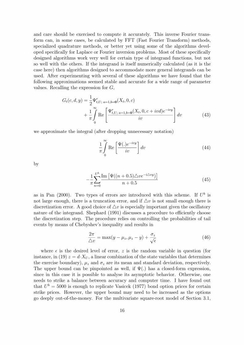
and care should be exercised to compute it accurately. This inverse Fourier trans-form can, in some cases, be calculated by FFT (Fast Fourier Transform) methods,specialized quadrature methods, or better yet using some of the algorithms devel-oped specifically for Laplace or Fourier inversion problems. Most of these specificallydesigned algorithms work very well for certain type of integrand functions, but notso well with the others. If the integrand is itself numerically calculated (as it is thecase here) then algorithms designed to accommodate more general integrands can beused. After experimenting with several of these algorithms we have found that thefollowing approximations seemed stable and accurate for a wide range of parametervalues. Recalling the expression for G,

Gt(c, d, y) =1

2Ψrt,U; a=1,b=0(Xt, 0, c)

+1

π

∞Z0

Re

"Ψrt,U ; a=1,b=0(Xt, 0, c+ ivd)e

−ivy

iv

#dv (43)

we approximate the integral (after dropping unnecessary notation)

1

π

∞Z0

Re

·Ψ(.)e−ivy

iv

¸dv (44)

by

−1π

UbXn=0

Im£Ψ((n+ 0.5)4ve−i4vy)¤

n+ 0.5(45)

as in Pan (2000). Two types of errors are introduced with this scheme. If U b isnot large enough, there is a truncation error, and if 4v is not small enough there isdiscretization error. A good choice of4v is especially important given the oscillatorynature of the integrand. Shephard (1991) discusses a procedure to efficiently choosethe discretization step. The procedure relies on controlling the probabilities of tailevents by means of Chebyshev’s inequality and results in

2π

4v = max(y − µz, µz − y) +σz√²

(46)

where ² is the desired level of error, z is the random variable in question (forinstance, in (19) z = d·XU , a linear combination of the state variables that determinesthe exercise boundary), µz and σz are its mean and standard deviation, respectively.The upper bound can be pinpointed as well, if Ψ(.) has a closed-form expression,since in this case it is possible to analyse its asymptotic behavior. Otherwise, oneneeds to strike a balance between accuracy and computer time. I have found outthat U b = 5000 is enough to replicate Vasicek (1977) bond option prices for certainstrike prices. However, the upper bound may need to be increased as the optionsgo deeply out-of-the-money. For the multivariate square-root model of Section 3.1,

16

we use the following approximation due to Bohmann (1970) that is more suitable forcases in which the characteristic function of z is known in closed-form. Given thatthe exercise event for the option is indicated by d ·XU ≤ y, the probability of thisevent can be approximated by

P (z ≤ y) = hy

π+2

π

UbXu=1

sin(hyu)

uRe[Φ(hu)] (47)

where Φ(v) is the characteristic function of z. The discretization step, h, can again

be found from (47) above replacing y by ln³

Ka1(U,T )a2(U,T )a3(U,T )

´. However, although

less ad-hoc, choosing the upper bound is more problematic in this case, and requiressolving

¯Φ(hU b)

¯U b

=yhπ²

4(48)

for U b. There is no guarantee that the precision will increase as we increase the upper

bound. As the parameters (such as time to maturity, strike price, maturity of theunderlying bond etc.) defining the option to be valued change, the discretization stepand the upper bound have to be re-calculated. With an appropriate starting valuethat again needs to be adjusted as the fundamental parameters change, the nonlinearequation in (48) is solved by a procedure that combines the well-known bisection andsecant methods, and is very fast.

17

4 Results

In this section empirical results are presented and interpreted. The empirical analysismainly focuses on three issues: The sensitivity of the defaultable claim values toparameters characterising jump terms, the effects of the correlation between the creditspread and the riskless short rate on valuation, and a comparative study of theeffectiveness of dynamic hedging strategies. The characteristics of the defaultableclaims that have been analysed in this section are as follows: First, we consider adefaultable bond that promises to pay $1 at its maturity in two years. In fact, withoutloss of generality, all the bonds riskless or defaultable, considered in the empiricalsection as underlying to some derivative security or by themselves, have the samematurity of two years, the promised payoff of $1, and assumed to be zero-coupon.Second, in the analysis, a put option on the defaultable bond is considered. Theoption has six months to maturity and a strike price of 0.95. Such options provideprotection against both interest rate risk and credit risk, hence maybe expensive ifthe intention is to protect only against one type of risk. Third, we take up a specifictype of credit option particularly useful for bond issuers borrowing on a floating basis.This is a call option on an appropriately defined credit spread that determines thecredit risk premium that the bond issuer has to pay. If there is an increase in thiscredit spread, the issuer would face higher borrowing costs. However, these costsmay be eliminated if the bond issuer also holds the call option which will payoffover a certain spread threshold similar to the strike price of an ordinary call option.Of course, this payoff would be small, but can be adjusted by a simple multiplier.Without loss of generality we set this multiplier to 1, set the spread threshold to onepercent, and assume that the option maturity is six months. The last defaultablesecurity analysed is the so-called credit spread option which basically gives its holder,at the maturity of the option, the right to exchange the underlying defaultable bondfor an otherwise similar riskless bond. In the computations the exchange ratio is setto one, and the option maturity is again six months. Note that unless the underlyingdefaultable bond and the riskless bond are affected differently from interest rate risk,these options provide protection against credit risk. See Section 2.2 for mathematicalexpressions of the payoff functions for these credit derivatives.Figures 1-5 show how the values of the riskless and the defaultable bond change

with respect to changes in some of the parameters. As the intensity of the any typeof jump in this model increases, one would expect a reduction in bond prices due toa higher rate of discounting. In fact this is exactly what we observe except that theriskless bond value is not influenced by changes in spread jump intensity or size whichis obvious. Even the defaultable bond, however, is not very sensitive to changes inthe intensity of credit spread jumps. It seems that the jumps in interest rates aremore important to the valuation of defaultable bonds than the jumps in the creditspread itself, and this is so whether one considers the effects of intensity or jumpsizes. This can be deduced from the slopes of the dotted lines in figures 1,2,4, and 5.Figure 6 depicts the values of the riskless and the defaultable bond with respect tomaturity. One can observe that the difference in their values increases as maturityincreases, which is to be expected since the defaultable bond becomes more and more

18

likely to default as time passes. Figure 7 shows the relation between bond values andthe correlation of riskless interest rate and credit spread changes. The correlationcoefficient is perturbed by varying the values of the parameter ρ in the range [-2,2]while keeping the current values of the state variables and other parameters fixed. Itcan be seen that the correlation coefficient does not affect neither bond’s value overa wide range. As the correlation gets near to -1 or 1, however, there is a substantialincrease in the value of the both riskless and defaultable bonds. At times of marketturmoil, correlation is driven by in the changes of not one parameter only, but inseveral parameters. Moreover, the state variables may also change drastically. Tomake things worse, even the whole model driving security values may change. Hence,the analysis concerning correlation in this paper is only suggestive, and hopefully isa precursor to full-fledged studies on the issue of correlation.The next series of figures are concerned with the put option on a defaultable bond.

In Figure 8 we observe that the value of the put option is actually more sensitive tothe intensity of jumps in credit spreads than that of the jumps in interest rates,which may, at a first glance, appear to be contradictory with figures 1-3. Note thatalthough an increase in interest rate jump intensity would decrease the value of thedefaultable bond, thus increasing the value of the put option; higher interest rateswould also mean higher discounting of the payoff thus reducing the value. The resultsso far indicate that although one may perhaps justify ignoring small jumps in creditspreads for the valuation of bonds, this omission would lead to considerable pricingerrors when one is interested in the valuation of a put option on a defaultable bond,or in any other option to generalize this insight. The interpretation of figures 9 and10 is straightforward in that any increase in mean jump sizes that would reduce thevalue of the underlying bond, is likely to increase the value of the put option. Figure11 shows the value of the put option with respect to correlation.10 The observationhere is that as the correlation gets near to -1 or 1 the value of the put option becomessmaller as the value of the underlying bond increases. At the most extremes, however,there is an increase in the value of the option. It remains to be seen whether thisis an artifact of parameter over-perturbation. The interesting result is that the putoption has its highest value for a correlation coefficient near zero. This makes senseas well since the underlying bond value is lowest around that range. Figures 12-14display the results for the call option on credit spread. As expected, an increasein spread jump intensity and/or size increases the value of the call option while anincrease in the same parameters for the interest rate jump decreases its value. Thisis because, unless the cash multiplier Q depends on the level of interest rates, theriskless interest rate serves only for discounting purposes for this type of derivative.It is also apparent that the value of the call option is much more sensitive to jumpsin credit spreads rather than those in the riskless interest rate, suggesting that, inthis case, discounting is of a secondary importance compared to the magnitude of theoption payoff. In addition, as the level above which we would like to insure increases(which means we are willing to absorb most of the credit risk ourselves) the value ofthe call option should decrease. This is observed in Figure 15. The value of the call

10This figure, along with most others, has been obtained by evaluating the relevant function overa small number of points. It has not been smoothed by interpolation to preserve its original shape.

19

option with respect to correlation is shown in Figure 16. It is evident that correlationdoes not influence much the value of the call option on credit spread. The payoff ofthis option is determined by how much the current level of the credit spread exceedsthe given threshold. The parameter ρ does not affect this payoff. Hence perturbingρ has an effect on the value of the call option only through its slight influence onthe riskless interest rate, that is, through discounting. The next set of figures areconcerned with the spread option. In Figure 17, it can be observed that an increasein the intensities of spread jumps, and common jumps (interest rate jumps) increase(decrease) the value of the spread option, though the reduction of value occurs at amuch lower rate. This should not be interpreted as to belittle the role of interest ratejumps in general. In this specific case, the effects, on the payoff of the option, of thesejumps cancel each other and only a small discounting effect remains. In other cases,payoff and discounting effects may work in the same direction. Indeed, when oneconsiders the effects of jump sizes rather than intensities, even the small discountingeffect mentioned before gets rather stronger as it is evident from Figure 18. Figure19, in turn, backs up Figure 17 in emphasizing the role of spread jumps, in thatthey increase the value of the option by decreasing the value of the defaultable bond.Obviously, if one expects increasing uncertainty regarding credit spreads, the right toexchange a defaultable bond for a pre-fixed number of riskless bonds become morevaluable. Figure 20 concludes our analysis of the sample credit derivatives. In thisfigure, it can be noted that the value of the spread option with respect to correlationis rather similar to that of bonds displayed in Figure 7. Nevertheless, to account forthe sharp increases in value at both extremes of the correlation range it should bethe case that the defaultable bond value increases less, relative to the riskless bondover this range, or that it is discounted even more heavily.In this part, we interpret the results of the dynamic hedging strategies details of

which have been outlined earlier in Section 3.2. We consider a trader who shorts aput option on the defaultable bond, and uses the proceeds of this sale to hedge hisposition. The option has six months to maturity, and a strike price of 0.95. Figure 21displays the results when he ignores the correlation. In Figure 22, he ignores credit riskaltogether and uses only treasury bonds for hedging. Although this may seem naive,low liquidity in defaultable corporate bonds may force the trader to do so. Whateverthe reason, undertaking such an analysis is useful in terms of quantifying the effects ofthis inefficient hedging strategy, and emphasizing the importance of credit risk froma hedging perspective. The values displayed in these figures are average absolutehedging errors. The trader may also be concerned with the magnitude of hedgingerrors with respect to the initial value of the put option. The values of the put optionfor various combinations of correlation defining parameters are shown in Table I.From figures 21, and 22, it can be noted that the hedging errors are much lower forthe trader ignoring the correlation between the credit spread and the riskless interestrate compared to those of the trader ignoring credit risk altogether. In Figure 21,it is interesting to note that when ρ1 + ρ2 = 0 the hedging errors are approximatelyzero. This makes sense since in this case the trader is essentially using the true modelto hedge the option. The disparity between the true model and the model that thetrader uses is largest when ρ1 + ρ2 is large. In our case, ρ1 and ρ2 are allowed to

20

vary between −1 and 1, so ρ1 + ρ2 = 2 is at a maximum. The hedging error for thiscase is largest as can be observed from Figure 21. Finally, figures 23, and 24 displaythe corresponding results for a put option that has a maturity of one year. As timeto maturity increases the errors seem to accumulate as it implied by the figures. Toresume the findings in this part: the empirical results indicate that hedging optionson defaultable corporate bonds using treasury bonds (thus ignoring credit risk) mayresult in large hedging errors, that ignoring correlation is also likely to lead to errors,though smaller in magnitude, and that as the time to maturity of the option to behedged increases hedging errors increase as well.

5 Conclusion

In this paper we have proposed a general framework for the valuation of default-able securities. The transform analysis used in the paper is its first application tothe valuation of credit risky securities. The proposed model is a multivariate affinestructure in which state variables follow jump-diffusion processes. Negative correla-tion between the credit spread and the riskless interest rate is allowed in the model,as well as time-varying conditional correlations and variances. The proposed affinestructure is admissible in the sense of Dai and Singleton (1999), and allows multipleeconomic interpretations for the state variables. Within this framework, defaultablebonds, a put option on the defaultable bond, a call option on the credit spread, and acredit spread option are valued. Valuation of vulnerable options is discussed as well.The model is calibrated to a cross-section of bond prices and sensitivity analysis isconducted with respect to parameters defining jump terms, and correlation. The per-formance of dynamic hedging strategies is analysed with respect to the correlationbetween the credit spread and the riskless interest rate. The results obtained showthat both types of jumps, spread and interest rate, can be important in the valuationof defaultable securities depending particularly on whether one is valuing a bond oran option on the bond. The effects of correlation on the values of credit derivativesare also quite context dependent. Nevertheless, the findings indicate that particularattention should be paid for extreme correlation coefficients for all cases, since theeffects on value may be enormous. The findings regarding the hedging strategiesshow that ignoring default risk in hedging options on defaultable bonds can lead tosubstantial hedging errors irrespective, largely, of the correlation structure in the truemodel. Errors, though smaller in magnitude, also follow if the correlation betweenthe riskless interest rate and the credit spread is ignored.

21

6 References

1. Akgun, A (2000). Model Risk with Jump Diffusions. pp. 181-207 in ModelRisk, (Edited by R.Gibson) Risk Publications.

2. Bakshi, G., and D.Madan (1999). Spanning and Derivative-Security Valuation.Forthcoming in the Journal of Financial Economics.

3. Bohmann, H (1970). A Method to Calculate the Distribution Function Whenthe Characteristic Function is Known. Nordisk Tidskr. Informationsbehandling10, 237-242.

4. Chen, R.R., and L.Scott (1995). Interest Rate Options in Multifactor Cox-Ingersoll-Ross Models of the Term Structure. Journal of Derivatives, Winter1995, 53.

5. Cox, J.C., J.E.Ingersoll, and S.A.Ross (1985). A Theory of the Term Structureof Interest Rates. Econometrica 53, 385-408.

6. Dai, Q., and K.Singleton (1999). Specification Analysis of Affine Term-StructureModels. Working Paper, Stanford University.

7. Das, S., and P.Tufano (1996). Pricing Credit-Sensitive Debt When InterestRates, Credit Ratings and Credit Spreads are Stochastic. Journal of FinancialEngineering 5, 161-198.

8. Duffee, G (1999). Estimating the Price of Default Risk. Review of FinancialStudies 12, 197-226.

9. Duffie, D (1996). Dynamic Asset Pricing Theory. Second Edition. PrincetonUniversity Press, Princeton, N.J.

10. Duffie, D., and R.Kan (1996). A Yield-Factor Model of Interest Rates. Mathe-matical Finance 6, 379-406.

11. Duffie, D., M.Schroder, and C.Skiadas (1996). Recursive Valuation of Default-able Securities and the Timing of Resolution of Uncertainty. Annals of AppliedProbability 6, 1075-1090.

12. Duffie, D., and K.Singleton (1999). Modeling Term Structures of DefaultableBonds. Review of Financial Studies.

13. Duffie, D., J.Pan, and K.Singleton (1999). Transform Analysis and OptionPricing for Affine Jump-Diffusions. Working Paper, Stanford University.

14. Heath D., R.Jarrow, and A.J.Morton (1992). Bond Pricing and the Term Struc-ture of Interest Rates: A New Methodology for Contingent Claims Valuation.Econometrica 60, 77-105.

22

15. Jarrow, R., and S.Turnbull (1995). Pricing Options on Financial SecuritiesSubject to Default Risk. Journal of Finance 50, 53-86.

16. Jarrow, R., D.Lando, and S.Turnbull (1997). A Markov Model for the TermStructure of Credit Spreads. Review of Financial Studies 10, 481-523.

17. Jarrow, R., and S.Turnbull (2000). The Intersection of Market and Credit Risk.Journal of Banking and Finance 24, 271-299.

18. Lando, D (1998). On Cox Processes and Credit Risky Securities. Review ofDerivatives Research 2, 99-120.

19. Longstaff, F.A., and E.S.Schwartz (1995). A Simple Approach to Valuing RiskyFixed and Floating Rate Debt. Journal of Finance 50, 789-820.

20. Merton, R.C (1974). On the Pricing of Corporate Debt: The Risk Structure ofInterest Rates. Journal of Finance 29, 449-470.

21. Milstein, G.N (1974). Approximate Integration of Stochastic Differential Equa-tions. Theory of Probability and Applications 19, 557-562.

22. Pan, J (2000). Integrated Time-Series Analysis of Spot and Option Prices.Working Paper, GSB, Stanford University.

23. Protter, P (1992). Stochastic Integration and Differential Equations. Springer-Verlag, Berlin.

24. Schonbucher, P (1998) Pricing Credit Risk Derivatives. Working Paper, Uni-versity of Bonn.

25. Shephard, N.G (1991). Numerical Integration Rules for Multivariate Inversions.Journal of Statistical Computation and Simulation 39, 37-46.

26. Vasicek, O.A (1977). An Equilibrium Characterisation of the Term Structure.Journal of Financial Economics 5, 177-188.

23

7 Appendix

Theorem 1 Generalized Multidimensional Ito lemma: Let X = (X1,X2, ...,Xn)be an n-tuple of semimartingales as specified in (3). Then f(Xt, t) is a semimartingaleand,

f(Xt, t) =

tZ0

fs(X, s)ds+

tZ0

fX(Xs, s) · dXcs +

1

2

tZ0

dXTs fXX(Xs, s)dXs

+

tZ0

[f(Xs + J, s)− f(Xs, s)] · dN(s) (49)

where Xc denotes the continuous part of the semimartingale, J shows a column ofthe jump size matrix J, and superscript T denotes the transpose operator.

Proof. See Protter (1992).

Theorem 2 Generalised Multidimensional Feynman-Kac: Let Xt be an n-dimensional jump-diffusion (more formally, a semimartingale) process as specified in(3). The ordinary Feynman-Kac theorem applies in this setting as well, taking intoaccount some additional technicalities. That is,

Df(x, t)−m(x, t)f(x, t) + h(x, t) = 0, (x,t) ∈ Rn × [0, T )with f(x, T ) = g(x). (50)

Then

f(x, t) = Ex,t

TZt

ϕt,sh(Xs, s)ds+ ϕt,Tg(XT )

with ϕt,s = exp

− sZt

m(Xu, u)du

(51)

iff f(x,t) is a solution to (50).

Proof. Proof. (Informal) Duffie (1996) proves the theorem for diffusions. Theextension to jump-diffusions follows by an appropriate manipulation of infinitesimalgenerators. Let Y(s) = f(Xs, s)ϕt,s for s ∈ [t, T ]. Then

dYs = [Dcf(Xs, s)−m(Xs, s)f(Xs, s)]ϕt,sds+ fX(Xs, s)σ(Xs, s)ϕt,sdW (s)

+ ϕt,s[f(Xs + J, s)− f(Xs, s)] · dN(s) (52)

where Dc denotes the continuous part of the generator, and J, as before, shows acolumn of the jump-size matrix J. Integrating (52), taking expectations, and arranging

24

yields

Ex,t[Y (T )] = f(x, t) + Ex,t

TZt

ϕt,s[Df(Xs, s)−m(Xs, s)f(Xs, s)]ds (53)

=⇒ f(x, t) = Ex,t

TZt

ϕt,sh(Xs, s)ds+ ϕt,Tg(XT )

(54)

where in going from (53) to (54) we have used (50).

Proof of (16): For ease of notation let Ψdt,T ; a=1,b=0(x, a0, b0) = φ(.) in (16). Then

φ(.) [α(t) + β(t) · x] should satisfy (11). HenceDΨdt,T ; a,b(x, a

0, b0) = Dφ(.)− r(x, t)φ(.) [α(t) + β(t) · x]+ φ(.) [αt(t) + βt(t) · x] + µ(x, t)φ(.)β(t)+ β(t)φX(.)σ(x, t)σ

T (x, t)

+LXj=1

λj(x, t)

ZΩ

£φ(x+ J j, .)β(t)J j

¤dF jJ(t) (55)

where

Dφ(.) = φt(.) + µ(x, t)φX(.) +1

2tr£φXX(.)σ(x, t)σ

T (x, t)¤

+LXj=1

λj(x, t)

ZΩ

£©φ(x+ J j, .)− φ(x, .)ª [α(t) + β(t) · x]¤ dF jJ(t) (56)

Using φ(.) = exp [α0(t) + β0(t) · x] , simplifying, and utilising the affine formulationsin (4) through (8), yields the ODEs in (17), and (18).

Identification of the Riccati Equations:For the empirical analysis we specialize the more general theoretical framework of

Section 1. The benchmark model laid out in Section 3 necessitates that we rewritethe two sets of Riccati equations derived in Section 1 in terms of the benchmarkmodel. This is done in the following. Note first that the dynamics of the three statevariables in the benchmark model can be rewritten as follows:

d

X1(t)X2(t)X3(t)

=

k1 0 00 k2 00 0 k3

θ1 −X1(t)θ2 −X2(t)−X3(t)

dt+

η1 0 00 η2 00 ρ 1

pX1(t) 0 0

0pX2(t) 0

0 0pγX2(t)

dW1(t)dW2(t)dW3(t)

+

Js(t) 0 Jsc(t)0 0 00 Jr(t) Jrc(t)

dNλss (t)

dNλrr (t)

dNλ(t)

(57)

25

This along with (4) through (8) yield

µ0(t) =

k1θ1k2θ20

, µ1(t) = −k1 0 0

0 −k2 00 0 −k3

(58)

σ0(t) = 03∗3, σ11(t) =

η21 0 00 0 00 0 0

, σ21(t) = 0 0 00 η22 ρη20 ρη2 γ + ρ2

, σ31(t) = 03∗3(59)

σ(x, t)σT (x, t) =

η21X1 0 00 η22X2 ρη2X20 ρη2X2 (γ + ρ2)X2

(60)

r0(t) = r0, r1(t) = [0, 1, 1]; s0(t) = s0, s1(t) = [1, 1, 0] (61)

R0(t) = r0 + s0, R1(t) = [1, 2, 1]; (62)

since R(x, t) = R0(t) +R1(t) · x = r(x, t) + s(x, t).To obtain the ODEs in their final form we also need to compute the Laplace

transform of jump sizes. This is done below by assuming normal univariate andbivariate distributions with parameters to be gleaned from the context. Define thefollowing:

Λ(u;X) =

ZΩ

euXdFX , (63)

Λ(u, v;X,Y ) =

ZΩ

euX+vY dFX,Y (64)

Λ0(u, u0;X) =ZΩ

euXu0XdFX (65)

Λ0(u, v, u0, v0;X,Y ) =ZΩ

euX+vY (u0X + v0Y )dFX,Y (66)

Λ(β 01(t); Js(t)) = exp·β 01(t)µJs +

1

2(β 01(t))

2σ2Js

¸(67)

Λ(β 03(t); Jr(t)) = exp·β 03(t)µJr +

1

2(β 03(t))

2σ2Jr

¸(68)

Λ(β 01(t), β03(t); Jsc(t), Jrc(t)) = exp [β

01(t)µJsc + β

03(t)µJrc]

exp

µ1

2

£(β01(t))

2σ2Jsc + (β03(t))

2σ2Jrc¤¶

exp (β01(t)β03(t)σJscσJrcρJ) (69)

26

Λ0(β01(t), β1(t); Js(t)) = β1(t)£µJs + β

01(t)σ

2Js

¤Λ(β01(t); Js(t))

Λ0(β03(t), β3(t);Jr(t)) = β3(t)£µJs + β

03(t)σ

2Jr

¤Λ(β 03(t);Jr(t))

Λ0(β 01(t), β03(t), β1(t),β3(t); Jsc(t), Jrc(t)) = Λ(β

01(t),β

03(t); Jsc(t), Jrc(t))

β1(t)Λ001(t) + β3(t)Λ002(t) (70)

with

Λ001(t) =£µJsc + β

01(t)σ

2Jsc + β

03(t)σJscσJrcρJ

¤Λ003(t) =

£µJrc + β

03(t)σ

2Jrc + β

01(t)σJscσJrcρJ

¤.

∂

∂tα0(t) = r0 + s0 − k1θ1β01(t)− k2θ2β 02(t)

+ λ10 [1− Λ(β 01(t);Js(t))]+ λ20 [1− Λ(β 03(t);Jr(t))]+ λ30 [1− Λ(β 01(t),β 03(t); Jsc(t), Jrc(t))]

with α0(T ) = a0. (71)

∂

∂tβ 01(t) = 1 + k1β

01(t)−

1

2(η1β

01(t))

2

+ λ1,(1)1 [1− Λ(β 01(t); Js(t))]

+ λ2,(1)1 [1− Λ(β 03(t); Jr(t))]

+ λ3,(1)1 [1− Λ(β 01(t), β03(t); Jsc(t), Jrc(t))]

with β 01(T ) = b01. (72)

∂

∂tβ02(t) = 2 + k2β

02(t)−

1

2(η2β

02(t))

2 − ρη2β 02(t)β03(t)−1

2[ρ2 + γ](β03(t))

2

+ λ1,(2)1 [1− Λ(β01(t); Js(t))]

+ λ2,(2)1 [1− Λ(β03(t); Jr(t))]

+ λ3,(2)1 [1− Λ(β01(t), β 03(t);Jsc(t), Jrc(t))]

with β 02(T ) = b02. (73)

∂

∂tβ 03(t) = 1 + k3β

03(t)

+ λ1,(3)1 [1− Λ(β 01(t); Js(t))]

+ λ2,(3)1 [1− Λ(β 03(t); Jr(t))]

+ λ3,(3)1 [1− Λ(β 01(t), β03(t); Jsc(t), Jrc(t))]

with β 03(T ) = b03. (74)

27

− ∂∂tα(t) = k1θ1β1(t) + k2θ2β2(t)

+ λ10Λ0(β01(t), β1(t); Js(t))

+ λ20Λ0(β03(t), β3(t); Jr(t))

+ λ30Λ0(β01(t), β

03(t), β1(t),β3(t); Jsc(t), Jrc(t))

with α(T ) = a. (75)

− ∂∂tβ1(t) = −k1β1(t) + η21β01(t)β1(t)

+ λ1,(1)1 Λ0(β 01(t), β1(t); Js(t))

+ λ2,(1)1 Λ0(β 03(t), β3(t); Jr(t))

+ λ3,(1)1 Λ0(β 01(t), β

03(t), β1(t),β3(t); Jsc(t), Jrc(t))

with β1(T ) = b1. (76)

− ∂∂tβ2(t) = −k2β2(t) + η22β 02(t)β2(t) + ρη2[β2(t)β 03(t) + β02(t)β3(t)]

+ [ρ2 + γ]β 03(t)β3(t)

+ λ1,(2)1 Λ0(β 01(t), β1(t); Js(t))

+ λ2,(2)1 Λ0(β 03(t), β3(t); Jr(t))

+ λ3,(2)1 Λ0(β 01(t), β

03(t), β1(t),β3(t); Jsc(t), Jrc(t))

with β2(T ) = b2. (77)

− ∂∂tβ3(t) = −k3β3(t)

+ λ1,(3)1 Λ0(β 01(t), β1(t); Js(t))

+ λ2,(3)1 Λ0(β 03(t), β3(t); Jr(t))

+ λ3,(3)1 Λ0(β 01(t), β

03(t), β1(t),β3(t); Jsc(t), Jrc(t))

with β3(T ) = b3. (78)

Admissibility of the Benchmark Model:In this section we show that our benchmark model is a special case of the maximal

admissible model defined in Dai and Singleton (1999) hence it is itself admissible. Todo this we begin by reproducing the canonical representation of an admissible affinemodel as laid out by Dai and Singleton (1999) in their own notation. Let the vectorof state variables dynamics be defined by

dY (t) = K(Θ− Y (t))dt+ ΣpS(t)dW (t) (79)

where W (t) is a N-dimensional vector of independent standard Brownian motionsand S(t) is a diagonal matrix with the ith diagonal element given by [S(t)]ii = αi +

28

β 0iY (t). For an arbitrary choice of the parameter vector ψ = (K,Θ,Σ, β,α) whereβ = (β1, ..., βN) denotes the matrix of coefficients on Y (t). A specification of ψ isadmissible if the resulting [S(t)]ii are strictly positive, for all i. Note that admissibilityis a feature that refers to conditional variances, hence we do not need concern ourselveswith a jump-diffusion model here as jumps will have no effect on the positivity ofconditional variance terms though they will surely change the set of solutions to thegoverning SDEs. Existence and uniqueness of solutions for SDEs characterised byjump-diffusion processes is a more general issue and beyond the scope of this paper.Let m = rank(β) index the degree of dependence of the conditional variances on thenumber of state variables. Then each affine structure within the family of admissibleN-factor affine models can be classified uniquely into one of N+1 sub-families basedon its value of m. Denote those N-factor affine structures with index value m that areadmissible by Am(N). Now, for each m partition Y (t) as Y 0 = (Y B

0, Y D

0) where Y B

is m × 1 and Y D is (N −m) × 1 and define the canonical representation of Am(N)

with K =

·KBBm×m 0m×(N−m)

KDB(N−m)×m KDD

(N−m)×(N−m)

¸for m > 0, Θ =

·ΘBm×10(N−m)×1

¸, Σ = I,

α =

·0m×1

1(N−m)×1

¸, β =

·Im×m βDBm×(N−m)

0(N−m)×m 0(N−m)×(N−m)

¸with the following restric-

tions: KiΘ =mPj=1

KijΘj > 0, 1 ≤ i ≤ m, Kij ≤ 0, 1 ≤ j ≤ m, j 6= i, Θi ≥ 0,

1 ≤ i ≤ m, βij ≥ 0, 1 ≤ i ≤ m, m + 1 ≤ j ≤ N. This canonical representation isadmissible and maximal in the sense that, given m, only minimal sufficient condi-tions for admissibility and minimal normalizations for econometric identification areimposed. (See the appendix in Dai and Singleton (1999) for the proof that theseconditions are indeed sufficient.) In the case where N = 3, and m = 2 their analysisshows that the following model is equivalent to the canonical model through invarianttransformations of parameters.

d

Y1(t)Y2(t)Y3(t)

=

K11 K12 0K21 K22 00 0 K33

Θ1 − Y1(t)Θ2 − Y2(t)−Y3(t)

dt+

1 0 00 1 0σ31 σ32 1

pS11(t) 0 0

0pS22(t) 0

0 0pS33(t)

dW1(t)dW2(t)dW3(t)

(80)

where S11(t) = β11(t)Y1(t), S22(t) = β22(t)Y2(t), S33(t) = α3+ β31Y1(t) + β32Y2(t).Now setting α3 = 0, β31 = 0, σ31 = 0, K12 = 0, K21 = 0 we obtain a model

that is again admissible since the latter is a subset of the first one. Finally, changingthe notation back to our paper and by setting β11 = η21, β22 = η22, the equivalencebetween the diffusion part of (57) and the subset model derived above is established.Since k1, k2, θ1, θ2, and γ are all greater than zero it is straightforward to verify thatthe aforementioned additional parameter restrictions are also satisfied.

29

Could State Variables Take Negative Values?In this section we take up the issue of the signs of the state variables. Recall that

the diffusion part of the benchmark model is guaranteed to be positive, but with thepresence of jump terms with normally distributed jump sizes there is a theoreticalpossibility that the first and the third state variables will take negative values. Wewould like to show that such an event can happen only with a very small probability.Empirically this would not pose much of a problem since parameters of the benchmarkmodel is estimated from real world data and we do not observe negative interest ratesnor negative credit spreads in financial markets. Hence it is to be expected that theparameter estimates reflect this information and the state variables identified as suchnever take negative values. To conduct our analysis we take up credit spreads andshow that they can become negative only with small probabilities. The case andargumentation for interest rates is the same and not repeated here. Recall that

dX1(t) = k1(θ1 −X1(t))dt+ η1pX1(t)dW1(t)

+ Js(t)dNλss (t) + Jsc(t)dN

λ(t) (81)

dX2(t) = k2(θ2 −X2(t))dt+ η2pX2(t)dW2(t) (82)

s(t) = s0 +X1(t) +X2(t) (83)

Integrating (81) gives

X1(t) = X1(0) + k1

θ1t− tZ0

X1(u)du

+ η1 tZ0

pX1(u)dW1(u)

+ JsNλss (t) + JscN

λ(t) (84)

where we have eliminated the dependence of jump size terms on time since in theempirical analysis we assume that jump sizes are identically distributed over time.Taking expectations (assuming the market is risk-neutral11),

EX1(t) = X1(0) + k1

θ1t− tZ0

EX1(u)du

+ µJsλst+ µJscλt (85)

and differentiating with respect to t,

∂EX1(t)

∂t= k1 [θ1 −EX1(t)] + µJsλs + µJscλ (86)

Solving this differential equation gives

EX1(t) =

µX1(0)− Z

k1

¶e−k1t +

Z

k1(87)

11This is necessary only if we want to make reference to real world credit spreads. If we areonly interested in checking whether the processes for X1 and s can take negative values then theassumption of market neutrality can be dispensed with.

30

where Z = k1θ1+µJsλs+µJscλ.We now obtain the variance ofX1(t) by a similar but amore involved way. Applying the generalized Ito lemma toX2

1 (t), taking expectations,and noting the independence between jump size, Poisson, and Brownian motions weget

EX21 (t) = X

21 (0) + (2Z + η

21)

tZ0

EX1(u)du

− 2k1tZ0

EX21 (u)du+ E(J

2s )λst+ E(J

2sc)λt (88)

Differentiating with respect to t, and substituting EX1(u) from above gives

∂EX21 (t)

∂t= (2Z + η21)

·µX1(0)− Z

k1

¶e−k1t +

Z

k1

¸− 2k1EX2

1 (t) + (σ2Js + µ

2Js)λs + (σ

2Jsc + µ

2Jsc)λ (89)

Solving this differential equation yields

EX21 (t) = X

21 (0)e

−2k1t +1− e−2k1t2k1

A+e−k1t − e−2k1t

k1B (90)

where

A = (σ2Js + µ2Js)λs + (σ

2Jsc + µ

2Jsc)λ+ (2Z + η

21)Z

k1

and

B = (2Z + η21)

µX1(0)− Z

k1

¶Finally, subtracting [EX1(t)]

2 from (90) we obtain the variance as

V ar[X1(t)] =η21k1

·X1(0)

¡e−k1t − e−2k1t¢+ Z

2k1

¡1− e−k1t¢2¸

+1− e−2k1t2k1

£(σ2Js + µ

2Js)λs + (σ

2Jsc + µ

2Jsc)λ

¤(91)

The mean and the variance of X2(t) is found by setting Z = k2θ2 and λs = 0, λ = 0in the above formulas, and are not displayed here. The mean of the credit spread isthen

E[s(t)] = s0 +

µX1(0)− θ1 − µJsλs + µJscλ

k1

¶e−k1t + θ1 +

µJsλs + µJscλ

k1

+ (X2(0)− θ2) e−k2t + θ2 (92)

31

and the variance is

V ar[s(t)] =η21k1

·X1(0)

¡e−k1t − e−2k1t¢+ k1θ1 + µJsλs + µJscλ

2k1

¡1− e−k1t¢2¸

+1− e−2k1t2k1

£(σ2Js + µ

2Js)λs + (σ

2Jsc + µ

2Jsc)λ

¤+η22k2

·X2(0)

¡e−k2t − e−2k2t¢+ θ2

2

¡1− e−k2t¢2¸ (93)

Substituting the estimated parameter values into (92) and (93) we find that theimplied standard deviation of the credit spread is very low compared to its mean asshown in the table below.

1 week 1 month 3 months 6 months 1 yearmean 0.0266 0.0275 0.0299 0.0331 0.0386stdev 0.0005 0.001 0.0016 0.0022 0.0029

For instance, one-month ahead mean of credit spread is 27 times bigger thanits standard deviation. That means that even for highly leptokurtic distributionsobserving negative credit spreads is very unlikely. By using Chebyshev’s inequality wecan actually pin down this probability even without knowing the true distribution ofs(t). This inequality states that for any random variable with finite variance (standarddeviation of s(t) converges to 0.0047 as t→∞)

Pr(|s− µ| > nσ) ≤ 1

n2(94)

For values of s below the mean we can take

Pr(s− µ < −nσ) ≤ 1

2n2(95)

where in fact the upper bound for the probability will be even smaller than thissince the distribution of credit spreads is expected to be positively skewed. In anycase putting n = 27.5 above yields 0.00066. This means that however leptokurticthe distribution is, as long as its variance is finite, the maximum probability the onemonth ahead credit spreads can become negative is 0.00066.

32

0 2 4 6 8 100.92

0.925

0.93

0.935

0.94

0.945

0.95

0.955

0.96Riskless Bond Defaultable Bond

Figure 1: Bond Value with respect to Spread Jump Intensity The intensity is on aper-year basis. Both bonds have two years to maturity, and promise to pay $1.

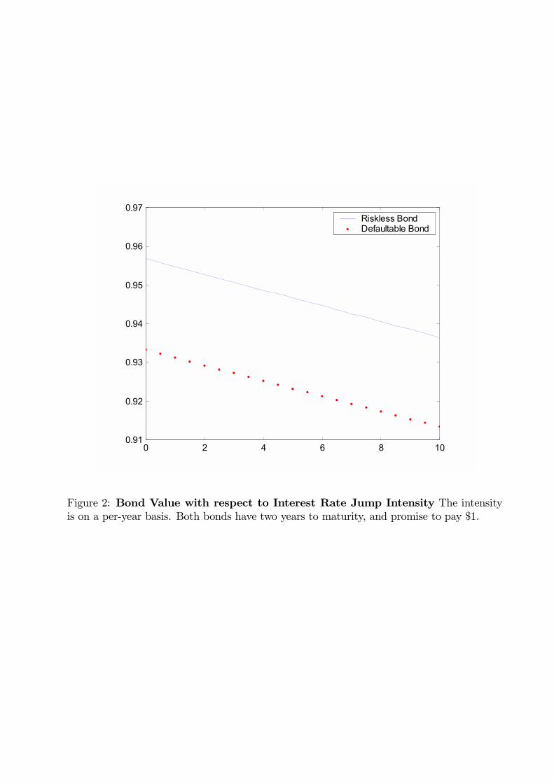
0 2 4 6 8 100.91

0.92

0.93

0.94

0.95

0.96

0.97Riskless Bond Defaultable Bond

Figure 2: Bond Value with respect to Interest Rate Jump Intensity The intensityis on a per-year basis. Both bonds have two years to maturity, and promise to pay $1.

0 2 4 6 8 100.92

0.925

0.93

0.935

0.94

0.945

0.95

0.955

0.96Riskless Bond Defaultable Bond

Figure 3: Bond Value with respect to Common Jump Intensity The intensity is ona per-year basis. Both bonds have two years to maturity, and promise to pay $1.

0 0.005 0.01 0.015 0.02 0.025 0.03 0.035 0.040.88

0.89

0.9

0.91

0.92

0.93

0.94

0.95

0.96Riskless Bond Defaultable Bond

Figure 4: Bond Value with respect to Mean Interest Rate Jump Size Both bondshave two years to maturity, and promise to pay $1.

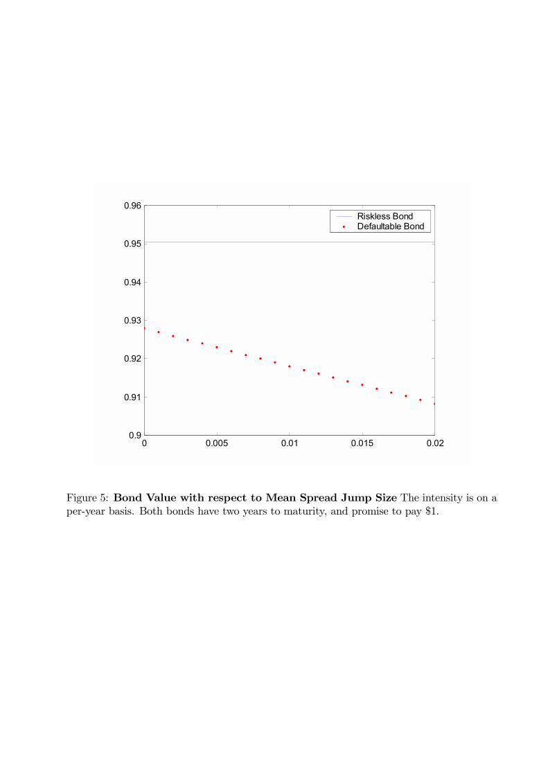
0 0.005 0.01 0.015 0.020.9

0.91

0.92

0.93

0.94

0.95

0.96Riskless Bond Defaultable Bond

Figure 5: Bond Value with respect to Mean Spread Jump Size The intensity is on aper-year basis. Both bonds have two years to maturity, and promise to pay $1.

0 2 4 6 8 100.3

0.4

0.5

0.6

0.7

0.8

0.9

1Riskless Bond Defaultable Bond

Figure 6: Bond Value with respect to Maturity The maturity is in years. Both bondshave two years to maturity, and promise to pay $1.

-1 -0.5 0 0.5 10.925

0.93

0.935

0.94

0.945

0.95

0.955

0.96

0.965Riskless Bond Defaultable Bond

Figure 7: Bond Value with respect to Correlation The maturity is in years. Bothbonds have two years to maturity, and promise to pay $1. Correlation is between theriskless interest rate and the credit spread changes.

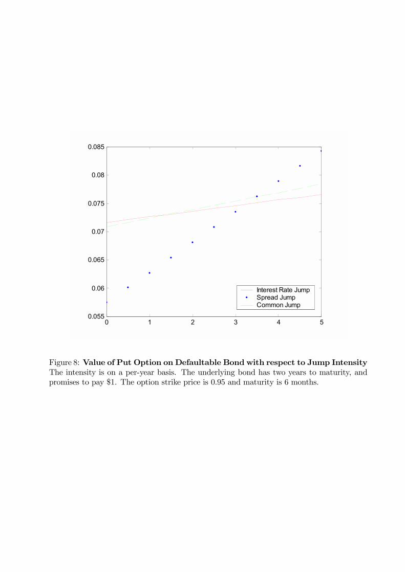
0 1 2 3 4 50.055

0.06

0.065

0.07

0.075

0.08

0.085

Interest Rate JumpSpread Jump Common Jump

Figure 8: Value of Put Option on Defaultable Bond with respect to Jump IntensityThe intensity is on a per-year basis. The underlying bond has two years to maturity, andpromises to pay $1. The option strike price is 0.95 and maturity is 6 months.

Figure 9: Value of Put Option on Defaultable Bond with respect to Mean InterestRate Jump Size The underlying bond has two years to maturity, and promises to pay $1.The option strike price is 0.95 and maturity is 6 months.

Figure 10: Value of Put Option on Defaultable Bond with respect to Mean SpreadJump Size The underlying bond has two years to maturity, and promises to pay $1. Theoption strike price is 0.95 and maturity is 6 months.

Figure 11: Value of Put Option on Defaultable Bond with respect to Correlation.The underlying bond has two years to maturity, and promises to pay $1. The option strikeprice is 0.95 and maturity is 6 months. Correlation is between the riskless interest rate andcredit spread changes.

Figure 12: Value of Call Option on Credit Spread with respect to Spread JumpIntensity The intensity is on a per-year basis, The option maturity is 6 months, withmultiplier Q=1, and spread threshold=0.01.

Figure 13: Value of Call Option on Credit Spread with respect to Mean InterestRate Jump Size The option maturity is 6 months, with multiplier Q=1, and spreadthreshold=0.01.

Figure 14: Value of Call Option on Credit Spread with respect to Mean SpreadJump Size The option maturity is 6 months, with multiplier Q=1, and spread thresh-old=0.01.

Figure 15: Value of Call Option on Credit Spread with respect to Spread Thresh-old The option maturity is 6 months, with multiplier Q set to 1.

Figure 16: Value of Call Option on Credit Spread with respect to Correlation. Theoption maturity is 6 months, with multiplier Q=1, and spread threshold=0.01. Correlationis between the riskless interest rate and credit spread changes.

0 1 2 3 4 50.042

0.043

0.044

0.045

0.046

0.047

0.048

0.049

Spread Jump Interest Rate JumpCommon Jump

Figure 17: Value of Spread Option with respect to Jump Intensity The intensityis on a per-year basis. Underlying bonds both have two years to maturity with $1 payoff.Exchange ratio is set to 1. Option maturity is 6 months.

Figure 18: Value of Spread Option with respect to Mean Interest Rate Jump SizeUnderlying bonds both have two years to maturity with $1 payoff. Exchange ratio is set to1. Option maturity is 6 months.

Figure 19: Value of Spread Option with respect to Mean Spread Jump Size Un-derlying bonds both have two years to maturity with $1 payoff. Exchange ratio is set to 1.Option maturity is 6 months.

Figure 20: Value of Spread Option with respect to Correlation Underlying bondsboth have two years to maturity with $1 payoff. Exchange ratio is set to 1. Option maturityis 6 months. Correlation is between the riskless interest rate and credit spread changes.

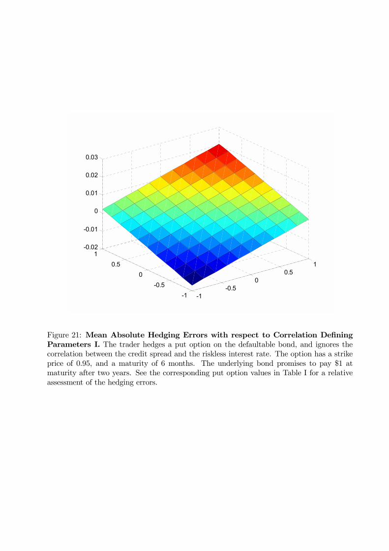
-1-0.5

00.5

1

-1-0.5

00.5

1-0.02

-0.01

0

0.01

0.02

0.03

Figure 21: Mean Absolute Hedging Errors with respect to Correlation DefiningParameters I. The trader hedges a put option on the defaultable bond, and ignores thecorrelation between the credit spread and the riskless interest rate. The option has a strikeprice of 0.95, and a maturity of 6 months. The underlying bond promises to pay $1 atmaturity after two years. See the corresponding put option values in Table I for a relativeassessment of the hedging errors.

-1-0.5

00.5

1

-1-0.5

00.5

1-0.01

0

0.01

0.02

0.03

0.04

Figure 22: Mean Absolute Hedging Errors with respect to Correlation DefiningParameters II. The trader hedges a put option on the defaultable bond, and totally ignoresdefault risk. The option has a strike price of 0.95, and a maturity of 6 months. Theunderlying bond promises to pay $1 at maturity after two years. See the corresponding putoption values in Table I for a relative assessment of the hedging errors.

-1-0.5

00.5

1

-1-0.5

00.5

1-0.03

-0.02

-0.01

0

0.01

0.02

0.03

Figure 23: Mean Absolute Hedging Errors with respect to Correlation DefiningParameters III. The trader hedges a put option on the defaultable bond, and ignores thecorrelation between the credit spread and the riskless interest rate. The option has a strikeprice of 0.95, and a maturity of 1 year. The underlying bond promises to pay $1 at maturityafter two years. See the corresponding put option values in Table I for a relative assessmentof the hedging errors.

-1-0.5

00.5

1

-1-0.5

00.5

1-0.01

0

0.01

0.02

0.03

0.04

0.05

Figure 24: Mean Absolute Hedging Errors with respect to Correlation DefiningParameters IV. The trader hedges a put option on the defaultable bond, and totallyignores default risk. The option has a strike price of 0.95, and a maturity of 1 year. Theunderlying bond promises to pay $1 at maturity after two years. See the corresponding putoption values in Table I for a relative assessment of the hedging errors.

Table I.

T=0.5 ρ1 / ρ2 -1 -0.75 -0.50 -0.25 0 0.25 0.50 0.75 1-1 0.0419 0.0445 0.0472 0.0498 0.0524 0.0550 0.0576 0.0601 0.0627

-0.75 0.0461 0.0487 0.0514 0.0540 0.0565 0.0591 0.0617 0.0642 0.0667-0.5 0.0503 0.0529 0.0555 0.0581 0.0607 0.0632 0.0657 0.0683 0.0708-0.25 0.0545 0.0571 0.0597 0.0622 0.0648 0.0673 0.0698 0.0723 0.0748

0 0.0586 0.0612 0.0638 0.0663 0.0688 0.0714 0.0738 0.0763 0.07880.25 0.0628 0.0653 0.0679 0.0704 0.0729 0.0754 0.0779 0.0803 0.08280.5 0.0669 0.0694 0.0719 0.0744 0.0769 0.0794 0.0819 0.0843 0.08670.75 0.0710 0.0735 0.0760 0.0785 0.0810 0.0834 0.0858 0.0883 0.0907

1 0.0751 0.0776 0.0800 0.0825 0.0850 0.0874 0.0898 0.0922 0.0946

T=1 ρ1 / ρ2 -1 -0.75 -0.50 -0.25 0 0.25 0.50 0.75 1-1 0.0565 0.0580 0.0596 0.0611 0.0626 0.0640 0.0655 0.0670 0.0684

-0.75 0.0607 0.0622 0.0637 0.0652 0.0667 0.0682 0.0696 0.0710 0.0725-0.5 0.0649 0.0664 0.0679 0.0694 0.0708 0.0722 0.0737 0.0751 0.0765-0.25 0.0691 0.0706 0.0720 0.0735 0.0749 0.0763 0.0777 0.0791 0.0805

0 0.0733 0.0747 0.0761 0.0776 0.0790 0.0804 0.0818 0.0832 0.08450.25 0.0774 0.0788 0.0802 0.0816 0.0830 0.0844 0.0858 0.0872 0.08850.5 0.0815 0.0829 0.0843 0.0857 0.0871 0.0884 0.0898 0.0911 0.09250.75 0.0856 0.0870 0.0884 0.0897 0.0911 0.0924 0.0938 0.0951 0.0964

1 0.0897 0.0911 0.0924 0.0938 0.0951 0.0964 0.0977 0.0990 0.1003

In this table, values of the put option on the defaultable bond are shown. The option has a strike of 0.95, and maturities of6 months, and 1 year respectively. The underlying bond pays $1 at the maturity of two years.

Put Option Values