Regime-Switching Perturbation for Non-Linear Equilibrium Models∗

Nelson Lind†

UC San Diego

October 10, 2014

Abstract

Salient macroeconomic problems often lead to highly non-linear models – for instance models incor-porating endogenous crises or the zero-lower-bound on interest. Accurately capturing non-linearity inequilibria often makes estimation infeasible. Local solution methods are limited since they struggle tocapture non-linearities, and the curse of dimensionality plagues global methods.

This paper introduces a local approach to solving highly non-linear models, generalizing perturbationto handle the class of piecewise smooth rational expectations models. First, I formalize the notion ofan endogenous regime by introducing a regime-switching equilibrium (RSE) concept. This frameworkuses non-linear model features to explain macroeconomic regime changes, and makes the distribution ofthe regime an equilibrium object instead of imposing an external regime-switching structure. Then, Idemonstrate how to apply perturbation within a slackened model and approximate the policy functionsassociated with a given belief about the regime. Finally, I solve for the equilibrium regime distributionusing backwards induction.

This approach (1) accounts for expectational effects due to the probability of regime change; (2) pro-vides a framework for modeling regime-switching from first principles; and (3) connects macroeconomictheory to reduced-form regime-switching econometric models.

∗I thank Brent Bundick, Jean Barthelemy, Davide Debortoli, James Hamilton, Marc Muendler, Valerie Ramey, IrinaTelyukova, Johannes Wieland, and seminar participants at the Banque de France, CEF 2014, Midwest Macro Spring 2014,and UCSD for comments and suggestions.†nrlind@ucsd.com, econweb.ucsd.edu/~nrlind, Dept. of Economics, University of California, San Diego, 9500 Gilman Dr

MC 0508, La Jolla, CA 92093-0508.

1

1 Introduction

Many salient macroeconomic problems are inherently non-linear1. Quantitatively realistic dynamic

stochastic general equilibrium (DSGE) models often require many state variables, and estimation based

on global solution techniques is typically infeasible due to the curse of dimensionality2. Instead, macroe-

conomists tend to rely on local methods to study medium and large scale models since they are fast and

standardizable3. But since these methods linearize equilibrium conditions, they are invalid for studying

highly non-linear models4.

Focusing on the class of piecewise smooth dynamic stochastic general equilibrium models, I introduce a

generalized perturbation technique to approximate regime-switching representations of rational expectations

equilibria. By overcoming the high cost of global methods and the limited applicability of perturbation

methods, this regime-switching perturbation method enables the study of general equilibrium models that

were previously considered intractable.

This method solves dynamic stochastic general equilibrium models whose structural equations are piece-

wise smooth5. This class includes business cycle models incorporating policy constraints like the zero-lower-

bound (Fernandez-Villaverde et al. (2012); Aruoba and Schorfheide (2012); Nakata (2012); Gavin et al.

(2013)), models of crises based on collateral constraints (Mendoza and Smith (2006); Mendoza (2010);

Korinek and Mendoza (2013)), and models of crises due to market breakdown (Boissay et al. (2013)). The

solution method only relies on the piecewise smooth structure of the model – which is known directly from

its equations – and does not rely on any information about how this non-linearity is reflected in equilibria.

A regime-switching characterization of rational expectations equilibrium underlies the solution method.

This alternative regime-switching equilibrium (RSE) concept uses regime-conditional solution functions and

specifies the distribution of the regime conditional on the state of the economy as an equilibrium object. I

show that it is equivalent to rational expectations equilibrium (REE) because both definitions of equilibrium

make identical in-equilibrium predictions. This result justifies using regime-switching representations of

equilibrium and provides a theoretical underpinning for regime-switching perturbation.

Introducing an endogenous regime is useful in models with strong non-linearities because the regime

variable can absorb non-smooth features. Once the model’s kinks and discontinuities are captured by the

regime, the model is everywhere smooth which enables a perturbation based solution method. Global

approaches for solving models incorporating the zero-lower-bound (ZLB) on interest rates (Gust et al. (2012);

1For instance, highly non-linear features arise in models of sovereign default (Arellano (2008), Mendoza and Yue (2012),Adam and Grill (2013)), the zero lower bound on interest rates (Fernandez-Villaverde et al. (2012), Aruoba and Schorfheide(2012), and Nakata (2012)), sudden stops (Mendoza (2010),Bianchi and Mendoza (2013),Korinek and Mendoza (2013)), andfinancial crises (Sannikov and Brunnermeier (2012), He and Krishnamurthy (2013), Gertler and Kiyotaki (2013), and Boissayet al. (2013)).

2See Gust et al. (2012) for a successful application of a global method in a model with three endogenous and three exogenousstate variables.

3See Jin and Judd (2002) and Schmitt-Grohe and Uribe (2004) for standard perturbation methods. Dynare (Adjemian et al.(2014)) provides a standardized solver. For recent local/perturbation methods for solving models with occasionally bindingconstraints see Brzoza-Brzezina et al. (2013) for a penalty function approach and Guerrieri and Iacoviello (2014) for a perfectforesight approach.

4Braun et al. (2012) show that economic conclusions can be very incorrect if log-linearization techniques are used inappro-priately in models incorporating the zero lower bound.

5Throughout I describe a real analytic function as a smooth function.

2

Aruoba and Schorfheide (2012); Fernandez-Villaverde et al. (2012)) also benefit from conditioning the solution

function on whether or not the ZLB binds, and I formalize this technique via an endogenous regime variable.

This idea is also central to the perfect foresight perturbation approach introduced by Guerrieri and

Iacoviello (2014). This important contribution demonstrates how local methods when coupled with a regime

structure can successfully approximate equilibria in ZLB models. However, the perfect foresight approach

means that the probability of transitioning between regimes does not influence the ultimate solution. The

RSE concept introduced in this paper incorporates the distribution of the regime explicitly as an equilibrium

object, which allows a researcher to account for expectational effects associated with regime changes when

solving the model with perturbation.

Prior solution approaches for DSGE models incorporating regime change specify the regime distribution

externally either as an exogenous Markov-switching process (as in Farmer et al. (2009); Bianchi (2012,

2013); Foerster (2013); Foerster et al. (2013)) or as a switching process that depends on the economy’s state

in a known way (as in Davig and Leeper (2006) or Barthelemy and Marx (2013)). This paper builds on

this literature by showing how to allow the evolution of the regime to come endogenously from the model

structure.

Instead of specifying how regimes evolve ex-ante, economists can explain the underlying reason for regime

change using first principles. First, the RSE concept formalizes how to incorporate a regime as an equilibrium

outcome. Then, by tying the realization of the regime in an RSE to non-linearity in theoretical models,

regime changes can be explained as coming from shifts in the fundamental structure of the economy. The

regime depends on economic fundamentals, and the distribution governing regime changes is an equilibrium

object. Previous regime-switching approaches emerge as the special case when evolution of the regime can

be determined ex-ante to solving the model6.

Incorporating an endogenous regime requires modifying typical perturbation procedures. Calculating

derivatives at a single steady state is no longer sufficient. Instead I show how to approximate RSEs relative

to regime dependent reference points. The procedure uses an augmented model which nests the original model

and a slack model via a perturbation parameter. The reference points solve the slack model, enabling an

application of the implicit function theorem to approximate solutions to the original model. This procedure

is closely related to solution methods for Markov-switching models. I show that solving for a first order

RSE can be accomplished by adapting techniques for Markov-switching rational expectations models such

as those in Farmer et al. (2011), Bianchi and Melosi (2012), Barthelemy and Marx (2013), Cho (2013), and

Foerster et al. (2013).

To solve for how the regime relates to the state of the economy, I use backwards induction. The per-

turbation step of the solution procedure relies on a guess of the regime distribution, but the distribution is

itself an equilibrium outcome. Since the regime is identified with the structure of the model – in particular

in what region current outcomes are realized – the distribution is restricted by the rational expectations

requirement. I show that a simple closed-form expression updates the distribution to be consistent with

6See appendix E.

3

solution function approximations.

The equilibrium representation and solution method provides a connection to linear regime-switching

models used routinely in time-series econometrics. In particular, a first order approximation of a regime-

switching equilibrium implies a linear state-space system for observable data. This result suggests that

macroeconomic processes which are well characterized by Markov-switching econometric models can be

modeled as resulting from regime-switching equilibria of non-linear DSGE models. Due to this connection,

the method provides a step towards empirical studies based on highly non-linear models – which are typically

infeasible since estimation exacerbates the computational burden of solving for equilibria.

Section 2 provides intuition for the technique by presenting a univariate model. I solve a special case of the

model directly, and show how the solution can be re-cast within a regime-switching structure. Finally, regime-

switching perturbation is applied to solve the model exactly. Section 3 presents the general case. I introduce

the class of piecewise smooth rational expectations models, the notion of regime-switching equilibrium, and

the general solution procedure. This section also contains equivalence results justifying the method. Section

4 returns to the example model and compares global solutions with the solutions calculated using regime-

switching perturbation. Section 5 concludes.

2 Example: A ZLB Model

This section works through a motivating example to fix ideas. The model incorporates the zero-lower-

bound (ZLB) on interest rates into a simple Fisherian model of inflation determination. A special case of the

model has closed-form solutions which take a piecewise linear form. I show how to re-express these equilibria

in a regime-switching linear form. In this representation, the regime variable indicates whether or not the

ZLB binds and the conditional distribution of the regime is an equilibrium object. Finally, I show how to

solve for the solution functions in this regime switching representation via perturbation.

The model consists of the Fisher equation relating nominal and real interest rates, and a ZLB-constrained

Taylor rule with interest rate persistence. This basic structure can be derived from a standard neoclassical

growth model with money and nominal bonds7.

rt = it − Etπt+1

rt = (1− ρr)r + ρrrt−1 + εt, εtiid∼ N (0, σ2)

i∗t = (1− ρi)r + ρii∗t−1 + θπt

it = max {0, i∗t }

(1)

The fisher equation defines the real interest rate rt as the nominal interest rate it net of expected inflation

Etπt+1. The real rate evolves as an exogenous AR(1) process with persistence of ρr. Monetary policy has a

desired nominal interest rate i∗t and sets the nominal interest rate it equal to this target whenever feasible.

Due to the zero lower bound, the central bank is constrained to setting the nominal rate at zero whenever

7See appendix F.

4

the desired rate is negative.

The desired rate is determined by a weighted average of all past deviations of inflation from the central

bank’s zero inflation target. As a result, i∗t can be interpreted as the central bank’s accumulated commitment

to make up for past deviations of inflation from this target. For example, if inflation has been below target

historically and the ZLB is binding, i∗t represents commitments to keep the interest rate low for an extended

period.

I assume that a Taylor-type principle holds and the reaction coefficient θ is positive and greater than

1−ρi. Under this assumption, the model has two steady states. The first corresponds to when policy achieves

its zero inflation target. The second is the Friedman steady state where the rate of deflation is equal to

the average real interest rate. Linear approximations based around either steady state are only valid if the

process for rt is sufficiently bounded to never push equilibrium outcomes across the kink generated by the

ZLB. Since the interesting case is precisely when the ZLB may occasionally bind, standard perturbation is

an inappropriate solution method.

2.1 Closed-Form Solution With ρr = 0

For the remainder of this section, I assume that the real interest rate has no persistence: ρr = 0. Under

this assumption, the model has a closed-form solution.

To solve the model, first reduce to a single equation in the desired rate by eliminating the real rate,

the realized nominal rate, and inflation. This reduction gives a single non-linear expectational difference

equation in the desired rate:

Eti∗t+1 = (1− ρi)r + max {ρii∗t , (ρi + θ)i∗t } − θrt (2)

The max operator arises from the ZLB constraint. When the desired rate is below zero, the ZLB binds, and

the right hand side has a slope of ρi < 1. When policy is not constrained by the ZLB, the slope is ρi+θ > 1.

Figure 1 depicts this equation and shows the two steady states of the model for comparison.

The only fundamental state variable in equation (2) is the exogenous shock, rt. A (recursive minimum-

state-variable) equilibrium is a map rt 7→ g(rt) = i∗t to determine the desired rate. Since rt is iid and the

future desired rate is determined by the same function in-equilibrium, the expected desired rate is constant

over time: Et [g(rt+1)] ≡ i∗e. Inverting the right hand side of (2) gives a piecewise linear expression for the

desired rate:

i∗t = g(rt) = min

{i∗e − (1− ρi)r + θrt

ρi,i∗e − (1− ρi)r + θrt

ρi + θ

}(3)

For any given level of i∗e, today’s desired rate is determined by one of two linear functions. The first corre-

sponds to when policy is constrained by the ZLB, and the second corresponds to when policy is unconstrained.

Regime-switching, whether or not the ZLB binds, is then just between one or the other entry.

In turn, since i∗e = Et [g(rt+1)], rational expectations requires that the expected desired rate must satisfy

5

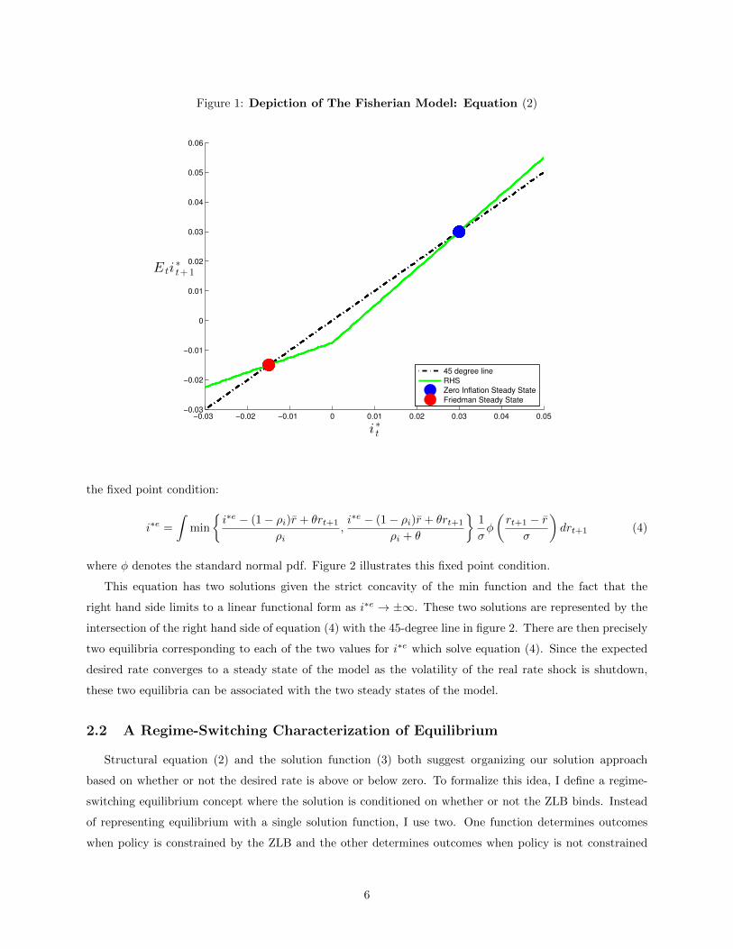
Figure 1: Depiction of The Fisherian Model: Equation (2)

−0.03 −0.02 −0.01 0 0.01 0.02 0.03 0.04 0.05−0.03

−0.02

−0.01

0

0.01

0.02

0.03

0.04

0.05

0.06

E ti∗

t+1

i∗

t

45 degree line

RHS

Zero Inflation Steady State

Friedman Steady State

the fixed point condition:

i∗e =

∫min

{i∗e − (1− ρi)r + θrt+1

ρi,i∗e − (1− ρi)r + θrt+1

ρi + θ

}1

σφ

(rt+1 − r

σ

)drt+1 (4)

where φ denotes the standard normal pdf. Figure 2 illustrates this fixed point condition.

This equation has two solutions given the strict concavity of the min function and the fact that the

right hand side limits to a linear functional form as i∗e → ±∞. These two solutions are represented by the

intersection of the right hand side of equation (4) with the 45-degree line in figure 2. There are then precisely

two equilibria corresponding to each of the two values for i∗e which solve equation (4). Since the expected

desired rate converges to a steady state of the model as the volatility of the real rate shock is shutdown,

these two equilibria can be associated with the two steady states of the model.

2.2 A Regime-Switching Characterization of Equilibrium

Structural equation (2) and the solution function (3) both suggest organizing our solution approach

based on whether or not the desired rate is above or below zero. To formalize this idea, I define a regime-

switching equilibrium concept where the solution is conditioned on whether or not the ZLB binds. Instead

of representing equilibrium with a single solution function, I use two. One function determines outcomes

when policy is constrained by the ZLB and the other determines outcomes when policy is not constrained

6

Figure 2: Fixed Point Condition For Rational Expectations: Equation (4)

−0.03 −0.02 −0.01 0 0.01 0.02 0.03 0.04 0.05−0.03

−0.02

−0.01

0

0.01

0.02

0.03

0.04

0.05

i∗e

i∗e

45 degree line

RHS

Zero Inflation Steady State

Friedman Steady State

by the ZLB. Note that distinguishing between these cases does not require any knowledge of the equilibria

of the model and only uses the information contained in the model’s structural equations.

Define a regime variable st which either takes a value of c when policy is constrained or u when policy

is unconstrained. Condition outcomes on this regime variable by defining two function gc and gu which

determine the desired rate depending on the prevailing regime. Since the regime is an endogenous outcome,

its probability law is an equilibrium object. Denote the distribution of st conditional on rt by Πs(r) ≡

P [st = s | rt = r].

To ensure that the regime variable correctly indicates when the ZLB binds, this conditional distribution

must be consistent with the equilibrium process for the desired rate. In particular, st = c can only occur

when the desired rate is below zero and st = u can only occur when the desired rate is above zero. This

means that the events {st = c and i∗t > 0} and {st = u and i∗t ≤ 0} must occur with probability zero and

are off-equilibrium path events.

In turn, if regime st = s does occur with positive probability given that rt = r, the model equation must

be satisfied:∫ ∑s′=c,u

gs′(r′)Πs′(r

′)σ−1φ(r′/σ)dr′ = (1− ρi)r + 1{st = c}ρigs(r) + 1{st = u}(ρi + θ)gs(r)− θr (5)

where I have used that i∗t ≤ 0 =⇒ st = c and i∗t > 0 =⇒ st = u. Note that this equation only must hold

7

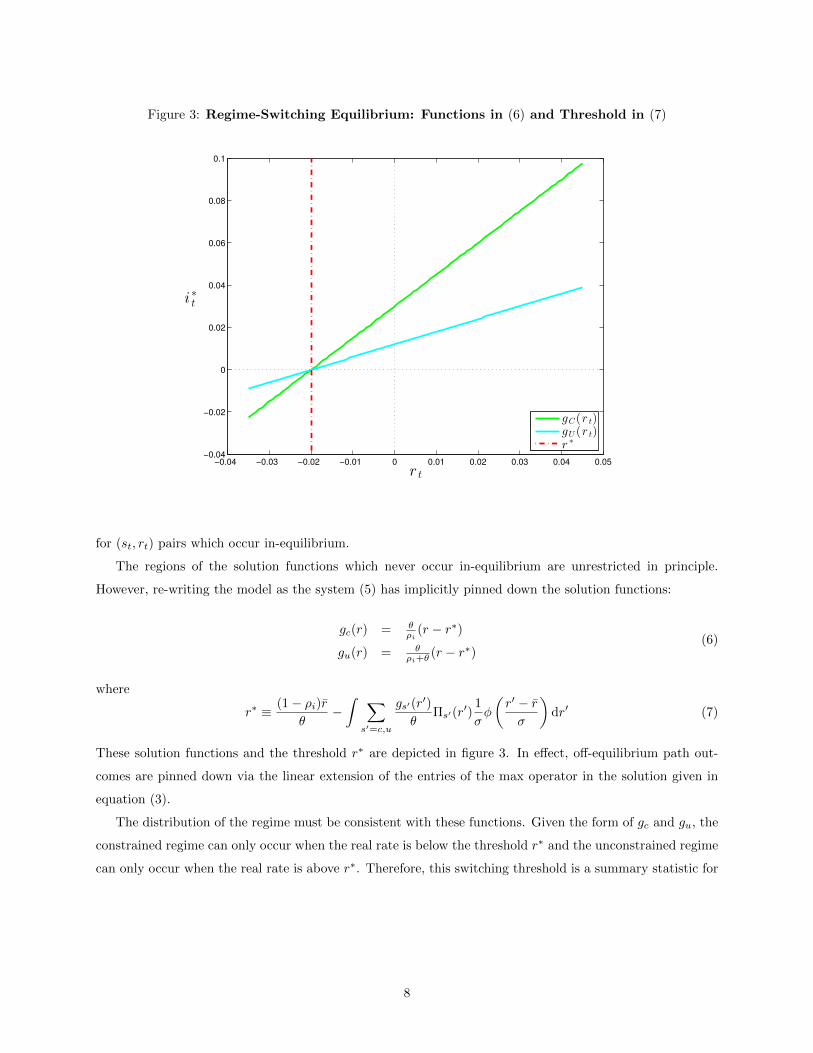
Figure 3: Regime-Switching Equilibrium: Functions in (6) and Threshold in (7)

−0.04 −0.03 −0.02 −0.01 0 0.01 0.02 0.03 0.04 0.05−0.04

−0.02

0

0.02

0.04

0.06

0.08

0.1

i∗t

r t

gC(r t)gU (r t)r ∗

for (st, rt) pairs which occur in-equilibrium.

The regions of the solution functions which never occur in-equilibrium are unrestricted in principle.

However, re-writing the model as the system (5) has implicitly pinned down the solution functions:

gc(r) = θρi

(r − r∗)

gu(r) = θρi+θ

(r − r∗)(6)

where

r∗ ≡ (1− ρi)rθ

−∫ ∑

s′=c,u

gs′(r′)

θΠs′(r

′)1

σφ

(r′ − rσ

)dr′ (7)

These solution functions and the threshold r∗ are depicted in figure 3. In effect, off-equilibrium path out-

comes are pinned down via the linear extension of the entries of the max operator in the solution given in

equation (3).

The distribution of the regime must be consistent with these functions. Given the form of gc and gu, the

constrained regime can only occur when the real rate is below the threshold r∗ and the unconstrained regime

can only occur when the real rate is above r∗. Therefore, this switching threshold is a summary statistic for

8

the equilibrium regime distribution:

Πs(r) =

1 {r ≤ r∗} if s = c

1 {r > r∗} if s = u(8)

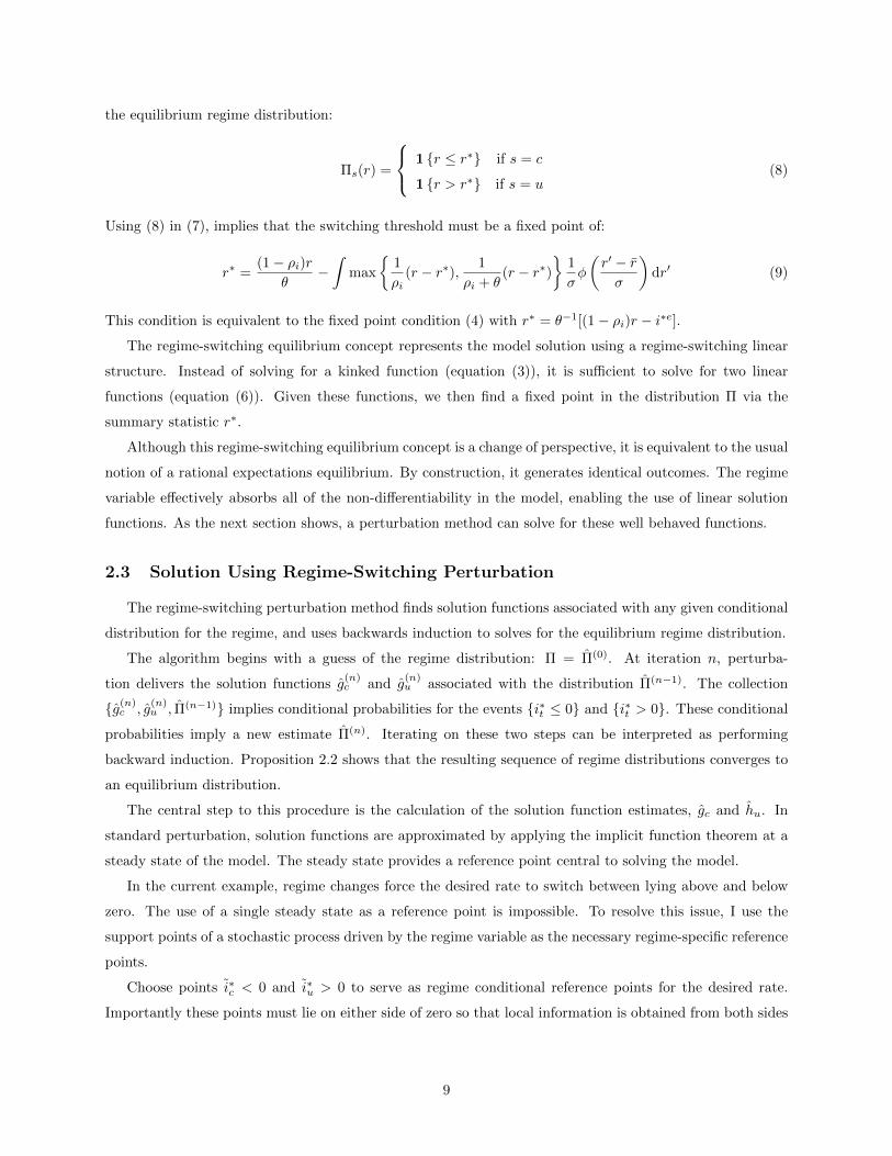
Using (8) in (7), implies that the switching threshold must be a fixed point of:

r∗ =(1− ρi)r

θ−∫

max

{1

ρi(r − r∗), 1

ρi + θ(r − r∗)

}1

σφ

(r′ − rσ

)dr′ (9)

This condition is equivalent to the fixed point condition (4) with r∗ = θ−1[(1− ρi)r − i∗e].

The regime-switching equilibrium concept represents the model solution using a regime-switching linear

structure. Instead of solving for a kinked function (equation (3)), it is sufficient to solve for two linear

functions (equation (6)). Given these functions, we then find a fixed point in the distribution Π via the

summary statistic r∗.

Although this regime-switching equilibrium concept is a change of perspective, it is equivalent to the usual

notion of a rational expectations equilibrium. By construction, it generates identical outcomes. The regime

variable effectively absorbs all of the non-differentiability in the model, enabling the use of linear solution

functions. As the next section shows, a perturbation method can solve for these well behaved functions.

2.3 Solution Using Regime-Switching Perturbation

The regime-switching perturbation method finds solution functions associated with any given conditional

distribution for the regime, and uses backwards induction to solves for the equilibrium regime distribution.

The algorithm begins with a guess of the regime distribution: Π = Π(0). At iteration n, perturba-

tion delivers the solution functions g(n)c and g

(n)u associated with the distribution Π(n−1). The collection

{g(n)c , g

(n)u , Π(n−1)} implies conditional probabilities for the events {i∗t ≤ 0} and {i∗t > 0}. These conditional

probabilities imply a new estimate Π(n). Iterating on these two steps can be interpreted as performing

backward induction. Proposition 2.2 shows that the resulting sequence of regime distributions converges to

an equilibrium distribution.

The central step to this procedure is the calculation of the solution function estimates, gc and hu. In

standard perturbation, solution functions are approximated by applying the implicit function theorem at a

steady state of the model. The steady state provides a reference point central to solving the model.

In the current example, regime changes force the desired rate to switch between lying above and below

zero. The use of a single steady state as a reference point is impossible. To resolve this issue, I use the

support points of a stochastic process driven by the regime variable as the necessary regime-specific reference

points.

Choose points i∗c < 0 and i∗u > 0 to serve as regime conditional reference points for the desired rate.

Importantly these points must lie on either side of zero so that local information is obtained from both sides

9

of the kink arising from the ZLB. Also, choose two reference points for the real rate: rc and ru8. Given these

points and a fixed regime distribution, define a slackness term as:

∆s,s′ = i∗s′ − (1− ρi)r −max{ρii∗s, (ρi + θ)i∗s

}+ θrs

The expected value of this slackness term is the residual in the model equation under the assumption that

outcomes are determined as (i∗t , rt) = (i∗st , rst) and st ∼∫

Πs(r + ε′)dF (ε′).

Next, augment the model with this slackness term using a nesting parameter η ∈ [0, 1]:

0 = Et[i∗t+1 − (1− ρi)r −max {ρii∗t , (ρi + θ)i∗t }+ θrt − (1− η)∆st,st+1

]rt+1 = (1− η)rst+1

+ η(r + εt+1), εt+1 ∼ N (0, σ2)

st+1 | εt+1 ∼ Πs(r + εt+1)

(10)

The first equation arises from appending the slack term (1 − η)∆s,s′ to equation (2). The second equation

specifies a distorted version of the real rate process. The evolution of the real rate is now a convex combination

of the reference point rs and the true process of the shock. Now both the regime variable and the Gaussian

innovation directly drive the real rate. Finally, the last line specifies that the regime is driven by the true

real rate process and not the modified real rate process.

This augmented model reduces to our original model when η = 1 because the residual term drops out

and the future real rate shock is no longer distorted towards the reference point rs′ . In the opposite case

with η = 0, the continuous shock does not impact the future value of the real rate which takes values of rc

and ru. In this slack model, the residual term enters fully and ensures that the reference points i∗c and i∗c

solve the model at the state-space points rc and ru. The slackened model distorts agent beliefs in such a

way to ensure that the chosen reference points solve the model.

Given fixed values for {Π, i∗c , i∗u, rc, ru}, a solution to this augmented model is a pair of functions gc(r, η)

and gu(r, η) such that model equation (10) is satisfied when i∗t = gst(rt, η) and i∗t+1 = gst+1(rt+1, η). Note

that these solutions now depend on the nesting parameter η.

Since the augmented model nests the original model, evaluating the solution functions gc(r, η) and gu(r, η)

at η = 1 gives the solution functions of the original model for a given conditional distribution Π. On the

other extreme, when η = 0 the augmented model reduces to the slack model. By construction, this slack

model has the chosen reference point as solution. The desired rate i∗c solves the augmented model at the

point (rs, 0):

i∗c = gc(rc, 0)

i∗u = gu(ru, 0)

Just as a deterministic steady state is the reference point for standard perturbation, the stochastic process

8In this example, these points can be arbitrary. Generally, it is helpful to choose them based on estimates of the regime-conditional means of the state variables of the model

10

(i∗st , rst) serves as a reference process. Now, an application of the implicit function theorem based on the

state-space points rc and ru (see appendix A) delivers the partial derivatives of the augmented model’s

solution functions.

Calculating these derivatives leads to a first order approximation:

gs(r, η) ≈ i∗s +∂

∂rg(rs, 0)(r − rs) +

∂

∂ηg(rs, 0)η

Setting η = 1 gives an approximate solution to the original model:

gs(r, 1) ≈[i∗s −

∂

∂rg(rs, 0)rs +

∂

∂ηgs(rs, 0)

]+

∂

∂rgs(rs, 0)r ≡ gs(r) (11)

Note that, the derivative with respect to η adjusts the constant term to account for the level shift introduced

by slackening the model.

In this example, the solution is linear so this approximation is in fact exact when Π is an equilibrium

conditional distribution. To arrive at this result, I use the following lemma which specifies the constants in

this approximation associated with any arbitrary choice of Π.

Lemma 2.1 For a given conditional distribution Π, not necessarily an equilibrium distribution, the constants

in the linear approximation (11) associated with Π are (s = u, c)[i∗s −

∂

∂rg(rs, 0)rs +

∂

∂ηgs(rs, 0)

]= as(Π) = −bsr∗(Π)

∂

∂rgs(rs, 0) = bs =

θρi

s = c

θρi+θ

s = u

where

r∗(Π) =

1−ρiθ r − Er′∼N (r,σ2)

[Πc(r

′) 1ρir′ + Πu(r′) 1

ρi+θr′]

1− Er′∼N (r,σ2)

[Πc(r′)

1ρi

+ Πu(r′) 1ρi+θ

]Proof. See appendix A.

The slope constant bs is the same slope constant in the true solution function given by equation (6). The

constant term depends on the regime distribution through the threshold r∗(Π). This threshold is the point

in the state space where both gc and gu equal zero9.

This lemma characterizes the solution delivered by using perturbation to approximate gc and gu holding

Π fixed. However, if Π is an equilibrium regime distribution, then the threshold r∗(Π) must be a threshold

which satisfies the fixed point condition (9). It immediately follows that this perturbation method delivers

the exact solution, as summarized in the following proposition:

9It is also a sufficient statistic for the conditional regime distribution implied by these functions

11

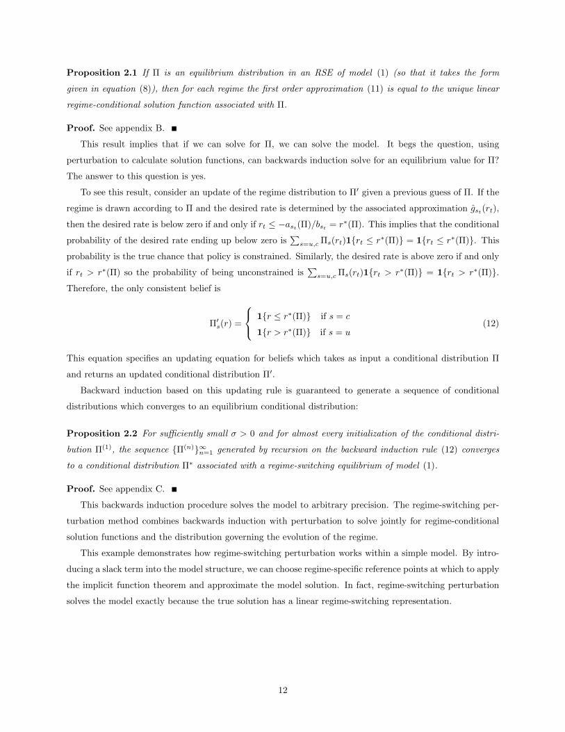
Proposition 2.1 If Π is an equilibrium distribution in an RSE of model (1) (so that it takes the form

given in equation (8)), then for each regime the first order approximation (11) is equal to the unique linear

regime-conditional solution function associated with Π.

Proof. See appendix B.

This result implies that if we can solve for Π, we can solve the model. It begs the question, using

perturbation to calculate solution functions, can backwards induction solve for an equilibrium value for Π?

The answer to this question is yes.

To see this result, consider an update of the regime distribution to Π′ given a previous guess of Π. If the

regime is drawn according to Π and the desired rate is determined by the associated approximation gst(rt),

then the desired rate is below zero if and only if rt ≤ −ast(Π)/bst = r∗(Π). This implies that the conditional

probability of the desired rate ending up below zero is∑s=u,c Πs(rt)1{rt ≤ r∗(Π)} = 1{rt ≤ r∗(Π)}. This

probability is the true chance that policy is constrained. Similarly, the desired rate is above zero if and only

if rt > r∗(Π) so the probability of being unconstrained is∑s=u,c Πs(rt)1{rt > r∗(Π)} = 1{rt > r∗(Π)}.

Therefore, the only consistent belief is

Π′s(r) =

1{r ≤ r∗(Π)} if s = c

1{r > r∗(Π)} if s = u(12)

This equation specifies an updating equation for beliefs which takes as input a conditional distribution Π

and returns an updated conditional distribution Π′.

Backward induction based on this updating rule is guaranteed to generate a sequence of conditional

distributions which converges to an equilibrium conditional distribution:

Proposition 2.2 For sufficiently small σ > 0 and for almost every initialization of the conditional distri-

bution Π(1), the sequence {Π(n)}∞n=1 generated by recursion on the backward induction rule (12) converges

to a conditional distribution Π∗ associated with a regime-switching equilibrium of model (1).

Proof. See appendix C.

This backwards induction procedure solves the model to arbitrary precision. The regime-switching per-

turbation method combines backwards induction with perturbation to solve jointly for regime-conditional

solution functions and the distribution governing the evolution of the regime.

This example demonstrates how regime-switching perturbation works within a simple model. By intro-

ducing a slack term into the model structure, we can choose regime-specific reference points at which to apply

the implicit function theorem and approximate the model solution. In fact, regime-switching perturbation

solves the model exactly because the true solution has a linear regime-switching representation.

12

3 The General Case

This section examines the concept of regime-switching equilibrium, and regime-switching perturbation.

The first sub-section specifies the general framework and the central assumption defining the class of piece-

wise smooth rational expectations models. The second sub-section provides equilibrium definitions and an

equivalence result that justifies focusing on regime-switching representations of rational expectations equi-

libria. The third sub-section examines the details of the method, and the fourth sub-section summarizes the

algorithm.

3.1 General Framework

Suppose a macroeconomic theory implies a model for a control variable vector Yt ∈ Y ⊂ RnY and state

variable vector Xt ∈ X ⊂ RnX which takes the form

0 = Etf(Yt+1, Yt, Xt, Xt)

Xt+1 = Xt + Σεt+1, εt+1iid∼ F

(13)

The vector Xt represents the pre-determined part of the state variables. The iid innovation, εt+1, introduces

a stochastic component to the state vector via the impact matrix Σ. Note that Σ may be singular so that

some state-variables are entirely pre-determined. I will refer to X as the state space, Y as the control space,

and Y× X as the outcome space of the model.

For instance, consider a real business cycle model with irreversible investment. Letting Ct, It, Kt, Nt, zt

denote consumption, investment, capital, labor, and log total factor productivity respectively, the model’s

equilibrium conditions are:

C−τt ≤ Λt ⊥ It ≥ 0

Λt = βEtC−τt+1

[1− δ + αezt+1

(Kt+1

Nt+1

)α−1]

Cτt1−Nt

= (1− α)ezt(Kt

Nt

)αeztKα

t N1−αt = Ct + It

Kt+1 = (1− δ)Kt + It

zt = ρzt−1 + εt

Here, Λt denotes the marginal utility from an increase in savings while εt is an exogenous iid innovation to

the log of total factor productivity.

The first equation defines a complementarity condition for whether or not investment is strictly positive

or constrained to equal zero. Investment is constrained when the marginal utility from savings is less than

the marginal utility from consumption.

13

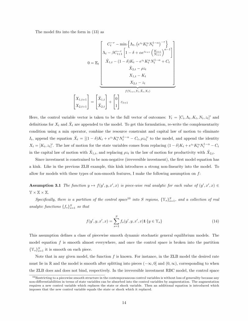
The model fits into the form in (13) as

0 = Et

C−τt −min{

Λt,(eztKα

t N1−αt

)−τ}Λt − βC−τt+1

[1− δ + αezt+1

(Kt+1

Nt+1

)α−1]

X1,t − (1− δ)Kt − eztKαt N

1−αt + Ct

X2,t − ρztX1,t −Kt

X2,t − zt

︸ ︷︷ ︸

f(Yt+1,Yt,Xt,Xt)X1,t+1

X2,t+1

=

X1,t

X2,t

+

0

1

εt+1

Here, the control variable vector is taken to be the full vector of outcomes: Yt = [Ct,Λt,Kt, Nt, zt]′ and

definitions for Xt and Xt are appended to the model. To get this formulation, re-write the complementarity

condition using a min operator, combine the resource constraint and capital law of motion to eliminate

It, append the equation Xt = [(1 − δ)Kt + eztKαt N

1−αt − Ct, ρzt]′ to the model, and append the identity

Xt = [Kt, zt]′. The law of motion for the state variables comes from replacing (1− δ)Kt + eztKα

t N1−αt −Ct

in the capital law of motion with X1,t, and replacing ρzt in the law of motion for productivity with X2,t.

Since investment is constrained to be non-negative (irreversible investment), the first model equation has

a kink. Like in the previous ZLB example, this kink introduces a strong non-linearity into the model. To

allow for models with these types of non-smooth features, I make the following assumption on f :

Assumption 3.1 The function y 7→ f(y′, y, x′, x) is piece-wise real analytic for each value of (y′, x′, x) ∈

Y× X× X.

Specifically, there is a partition of the control space10 into S regions, {Ys}Ss=1, and a collection of real

analytic functions {fs}Ss=1 so that

f(y′, y, x′, x) =

S∑s=1

fs(y′, y, x′, x)1 {y ∈ Ys} (14)

This assumption defines a class of piecewise smooth dynamic stochastic general equilibrium models. The

model equation f is smooth almost everywhere, and once the control space is broken into the partition

{Ys}Ss=1 it is smooth on each piece.

Note that in any given model, the function f is known. For instance, in the ZLB model the desired rate

must lie in R and the model is smooth after splitting into pieces (−∞, 0] and (0,∞), corresponding to when

the ZLB does and does not bind, respectively. In the irreversible investment RBC model, the control space

10Restricting to a piecewise smooth structure in the contemporaneous control variables is without loss of generality because anynon-differentiabilities in terms of state variables can be absorbed into the control variables by augmentation. The augmentationrequires a new control variable which replaces the state or shock variable. Then an additional equation is introduced whichimposes that the new control variable equals the state or shock which it replaced.

14

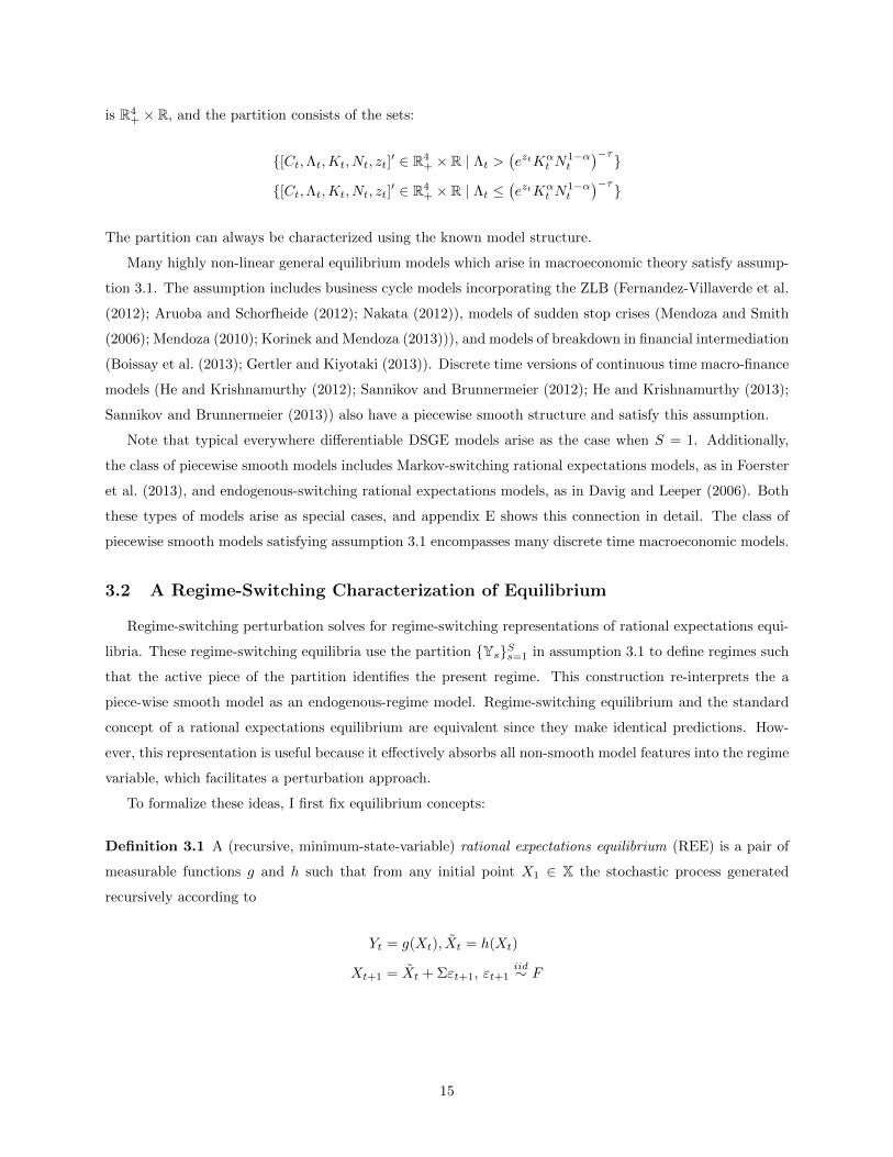
is R4+ × R, and the partition consists of the sets:

{[Ct,Λt,Kt, Nt, zt]′ ∈ R4

+ × R | Λt >(eztKα

t N1−αt

)−τ}{[Ct,Λt,Kt, Nt, zt]

′ ∈ R4+ × R | Λt ≤

(eztKα

t N1−αt

)−τ}The partition can always be characterized using the known model structure.

Many highly non-linear general equilibrium models which arise in macroeconomic theory satisfy assump-

tion 3.1. The assumption includes business cycle models incorporating the ZLB (Fernandez-Villaverde et al.

(2012); Aruoba and Schorfheide (2012); Nakata (2012)), models of sudden stop crises (Mendoza and Smith

(2006); Mendoza (2010); Korinek and Mendoza (2013))), and models of breakdown in financial intermediation

(Boissay et al. (2013); Gertler and Kiyotaki (2013)). Discrete time versions of continuous time macro-finance

models (He and Krishnamurthy (2012); Sannikov and Brunnermeier (2012); He and Krishnamurthy (2013);

Sannikov and Brunnermeier (2013)) also have a piecewise smooth structure and satisfy this assumption.

Note that typical everywhere differentiable DSGE models arise as the case when S = 1. Additionally,

the class of piecewise smooth models includes Markov-switching rational expectations models, as in Foerster

et al. (2013), and endogenous-switching rational expectations models, as in Davig and Leeper (2006). Both

these types of models arise as special cases, and appendix E shows this connection in detail. The class of

piecewise smooth models satisfying assumption 3.1 encompasses many discrete time macroeconomic models.

3.2 A Regime-Switching Characterization of Equilibrium

Regime-switching perturbation solves for regime-switching representations of rational expectations equi-

libria. These regime-switching equilibria use the partition {Ys}Ss=1 in assumption 3.1 to define regimes such

that the active piece of the partition identifies the present regime. This construction re-interprets the a

piece-wise smooth model as an endogenous-regime model. Regime-switching equilibrium and the standard

concept of a rational expectations equilibrium are equivalent since they make identical predictions. How-

ever, this representation is useful because it effectively absorbs all non-smooth model features into the regime

variable, which facilitates a perturbation approach.

To formalize these ideas, I first fix equilibrium concepts:

Definition 3.1 A (recursive, minimum-state-variable) rational expectations equilibrium (REE) is a pair of

measurable functions g and h such that from any initial point X1 ∈ X the stochastic process generated

recursively according to

Yt = g(Xt), Xt = h(Xt)

Xt+1 = Xt + Σεt+1, εt+1iid∼ F

15

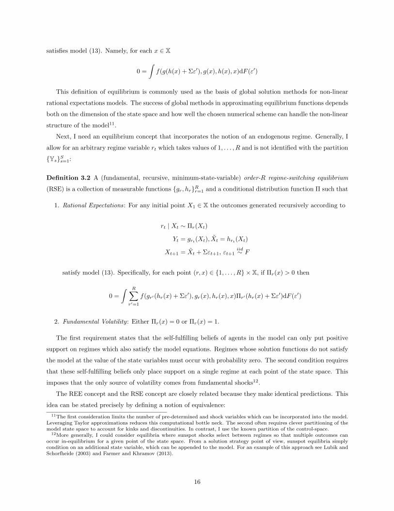
satisfies model (13). Namely, for each x ∈ X

0 =

∫f(g(h(x) + Σε′), g(x), h(x), x)dF (ε′)

This definition of equilibrium is commonly used as the basis of global solution methods for non-linear

rational expectations models. The success of global methods in approximating equilibrium functions depends

both on the dimension of the state space and how well the chosen numerical scheme can handle the non-linear

structure of the model11.

Next, I need an equilibrium concept that incorporates the notion of an endogenous regime. Generally, I

allow for an arbitrary regime variable rt which takes values of 1, . . . , R and is not identified with the partition

{Ys}Ss=1:

Definition 3.2 A (fundamental, recursive, minimum-state-variable) order-R regime-switching equilibrium

(RSE) is a collection of measurable functions {gr, hr}Rr=1 and a conditional distribution function Π such that

1. Rational Expectations: For any initial point X1 ∈ X the outcomes generated recursively according to

rt | Xt ∼ Πr(Xt)

Yt = grt(Xt), Xt = hrt(Xt)

Xt+1 = Xt + Σεt+1, εt+1iid∼ F

satisfy model (13). Specifically, for each point (r, x) ∈ {1, . . . , R} × X, if Πr(x) > 0 then

0 =

∫ R∑r′=1

f(gr′(hr(x) + Σε′), gr(x), hr(x), x)Πr′(hr(x) + Σε′)dF (ε′)

2. Fundamental Volatility : Either Πr(x) = 0 or Πr(x) = 1.

The first requirement states that the self-fulfilling beliefs of agents in the model can only put positive

support on regimes which also satisfy the model equations. Regimes whose solution functions do not satisfy

the model at the value of the state variables must occur with probability zero. The second condition requires

that these self-fulfilling beliefs only place support on a single regime at each point of the state space. This

imposes that the only source of volatility comes from fundamental shocks12.

The REE concept and the RSE concept are closely related because they make identical predictions. This

idea can be stated precisely by defining a notion of equivalence:

11The first consideration limits the number of pre-determined and shock variables which can be incorporated into the model.Leveraging Taylor approximations reduces this computational bottle neck. The second often requires clever partitioning of themodel state space to account for kinks and discontinuities. In contrast, I use the known partition of the control-space.

12More generally, I could consider equilibria where sunspot shocks select between regimes so that multiple outcomes canoccur in-equilibrium for a given point of the state space. From a solution strategy point of view, sunspot equilibria simplycondition on an additional state variable, which can be appended to the model. For an example of this approach see Lubik andSchorfheide (2003) and Farmer and Khramov (2013).

16

Definition 3.3 A REE (g, h) and an order-R RSE are equivalent equilibria if for each x ∈ X and each

r ∈ {1, . . . , R} if Πr(x) > 0 then gr(x) = g(x) and hr(x) = h(x).

An REE and an RSE are equivalent when they agree on contemporaneous outcomes across all points of the

state space.

The formal link between these equilibrium concepts is summarized in the following proposition:

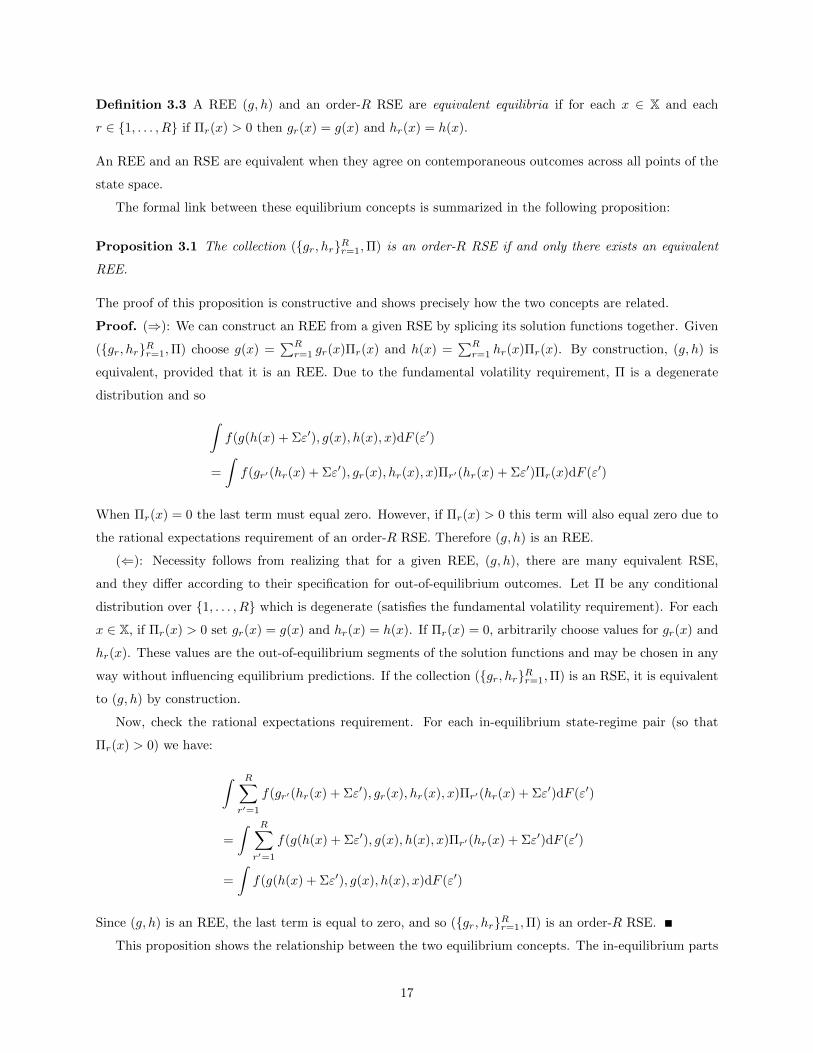
Proposition 3.1 The collection ({gr, hr}Rr=1,Π) is an order-R RSE if and only there exists an equivalent

REE.

The proof of this proposition is constructive and shows precisely how the two concepts are related.

Proof. (⇒): We can construct an REE from a given RSE by splicing its solution functions together. Given

({gr, hr}Rr=1,Π) choose g(x) =∑Rr=1 gr(x)Πr(x) and h(x) =

∑Rr=1 hr(x)Πr(x). By construction, (g, h) is

equivalent, provided that it is an REE. Due to the fundamental volatility requirement, Π is a degenerate

distribution and so ∫f(g(h(x) + Σε′), g(x), h(x), x)dF (ε′)

=

∫f(gr′(hr(x) + Σε′), gr(x), hr(x), x)Πr′(hr(x) + Σε′)Πr(x)dF (ε′)

When Πr(x) = 0 the last term must equal zero. However, if Πr(x) > 0 this term will also equal zero due to

the rational expectations requirement of an order-R RSE. Therefore (g, h) is an REE.

(⇐): Necessity follows from realizing that for a given REE, (g, h), there are many equivalent RSE,

and they differ according to their specification for out-of-equilibrium outcomes. Let Π be any conditional

distribution over {1, . . . , R} which is degenerate (satisfies the fundamental volatility requirement). For each

x ∈ X, if Πr(x) > 0 set gr(x) = g(x) and hr(x) = h(x). If Πr(x) = 0, arbitrarily choose values for gr(x) and

hr(x). These values are the out-of-equilibrium segments of the solution functions and may be chosen in any

way without influencing equilibrium predictions. If the collection ({gr, hr}Rr=1,Π) is an RSE, it is equivalent

to (g, h) by construction.

Now, check the rational expectations requirement. For each in-equilibrium state-regime pair (so that

Πr(x) > 0) we have:

∫ R∑r′=1

f(gr′(hr(x) + Σε′), gr(x), hr(x), x)Πr′(hr(x) + Σε′)dF (ε′)

=

∫ R∑r′=1

f(g(h(x) + Σε′), g(x), h(x), x)Πr′(hr(x) + Σε′)dF (ε′)

=

∫f(g(h(x) + Σε′), g(x), h(x), x)dF (ε′)

Since (g, h) is an REE, the last term is equal to zero, and so ({gr, hr}Rr=1,Π) is an order-R RSE.

This proposition shows the relationship between the two equilibrium concepts. The in-equilibrium parts

17

of an RSE’s solution functions always match with the solution functions of some REE. The out-of-equilibrium

parts of the functions gr and hr can never occur and do not influence equilibrium predictions. They are

completely unrestricted by the definition of an RSE, and we have many possible RSE’s simply by varying

out-of-equilibrium outcomes.

Since out-of-equilibrium events are unrestricted, we can focus attention on sub-classes of RSE’s by placing

restrictions on out-of-equilibrium outcomes. In the previous section, we used this idea to work exclusively

with linear solution functions. In the general case, we can focus on smooth solution functions due to

assumption 3.1.

This is accomplished by identifying each of the R regimes with a segment of the piece-wise smooth model.

This choice allows the regime variable to absorb all of the non-differentiable features in the model, effectively

converting it into a smooth model with an endogenous regime variable.

This idea can be formalized by defining a concept of partition consistency:

Definition 3.4 Given a control-space partition {Ys}Ss=1, an order-R RSE is partition consistent if for each

r ∈ {1, . . . , R} there exists some s ∈ {1, . . . , S} so that for every x ∈ X if Πr(x) > 0 then gr(x) ∈ Ys.

Partition consistency implies that each regime is tied to a unique piece of the natural partition arising from

the model’s structural equations. The outcomes generated by each regime must lie in a single piece of the

model’s partition, and so knowing the current regime implies knowing the active piece of the model partition.

But since the model is smooth on the interior of each piece Ys, this implies that each solution function

can be smoothly pinned down by the model structure while the regime stays fixed. To see this, fix the regime

at r and use assumption 3.1 and partition consistency of the RSE to write:

Πr(x) > 0 =⇒ 0 =

∫ R∑r′=1

f(gr′(hr(x) + Σε′), gr(x), hr(x), x)Πr′(hr(x) + Σε′)dF (ε′)

=

∫ R∑r′=1

S∑s=1

fs(gr′(hr(x) + Σε′), gr(x), hr(x), x)1{gr(x) ∈ Ys}Πr′(hr(x) + Σε′)dF (ε′)

=

∫ R∑r′=1

fs(r)(gr′(hr(x) + Σε′), gr(x), hr(x), x)Πr′(hr(x) + Σε′)dF (ε′)

where s : {1, . . . , r} → {1, . . . , S} is the map from the current regime to the currently active partition. This

mapping is well-defined because of partition consistency. The model is now entirely smooth, apart from any

non-smoothness arising from a perfectly forecastable jump in the future regime that could be enduced by

varying x. Provided that future regime changes are not extremely sensitive to current choices which determine

the state, the model is completely smooth, and it is reasonable to look for smooth regime-conditional solution

functions.

18

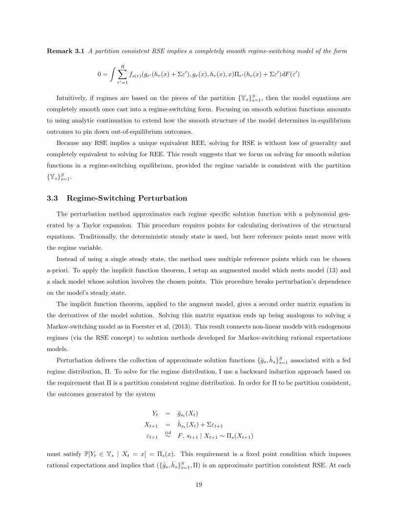
Remark 3.1 A partition consistent RSE implies a completely smooth regime-switching model of the form

0 =

∫ R∑r′=1

fs(r)(gr′(hr(x) + Σε′), gr(x), hr(x), x)Πr′(hr(x) + Σε′)dF (ε′)

Intuitively, if regimes are based on the pieces of the partition {Ys}Ss=1, then the model equations are

completely smooth once cast into a regime-switching form. Focusing on smooth solution functions amounts

to using analytic continuation to extend how the smooth structure of the model determines in-equilibrium

outcomes to pin down out-of-equilibrium outcomes.

Because any RSE implies a unique equivalent REE, solving for RSE is without loss of generality and

completely equivalent to solving for REE. This result suggests that we focus on solving for smooth solution

functions in a regime-switching equilibrium, provided the regime variable is consistent with the partition

{Ys}Ss=1.

3.3 Regime-Switching Perturbation

The perturbation method approximates each regime specific solution function with a polynomial gen-

erated by a Taylor expansion. This procedure requires points for calculating derivatives of the structural

equations. Traditionally, the deterministic steady state is used, but here reference points must move with

the regime variable.

Instead of using a single steady state, the method uses multiple reference points which can be chosen

a-priori. To apply the implicit function theorem, I setup an augmented model which nests model (13) and

a slack model whose solution involves the chosen points. This procedure breaks perturbation’s dependence

on the model’s steady state.

The implicit function theorem, applied to the augment model, gives a second order matrix equation in

the derivatives of the model solution. Solving this matrix equation ends up being analogous to solving a

Markov-switching model as in Foerster et al. (2013). This result connects non-linear models with endogenous

regimes (via the RSE concept) to solution methods developed for Markov-switching rational expectations

models.

Perturbation delivers the collection of approximate solution functions {gs, hs}Ss=1 associated with a fed

regime distribution, Π. To solve for the regime distribution, I use a backward induction approach based on

the requirement that Π is a partition consistent regime distribution. In order for Π to be partition consistent,

the outcomes generated by the system

Yt = gst(Xt)

Xt+1 = hst(Xt) + Σεt+1

εt+1iid∼ F , st+1 | Xt+1 ∼ Πs(Xt+1)

must satisfy P[Yt ∈ Ys | Xt = x] = Πs(x). This requirement is a fixed point condition which imposes

rational expectations and implies that ({gs, hs}Ss=1,Π) is an approximate partition consistent RSE. At each

19

iteration of the algorithm, I update the regime distribution based on the known partition {Ys}Ss=1 so that it is

consistent with solution function approximations. Using this distribution update step after each perturbation

step, gives a complete iteration of the solution algorithm.

This procedure amounts to performing backward induction on the conditional distribution of the regime.

Let an exponent of (n) denote an equilibrium object associated with the n-th iteration of the algorithm.

Then each iteration n consists of a perturbation step to find estimates {g(n)s , h

(n)s }Ss=1 given Π(n−1), and then

a distribution update step which calculates Π(n) given ({g(n)s , h

(n)s }Ss=1,Π

(n−1)). This generates a sequence

{Π(n)}. If this sequence converges, then the limit is an approximate equilibrium distribution.

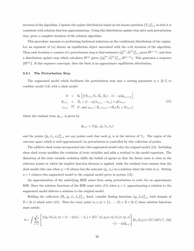
3.3.1 The Perturbation Step

The augmented model which facilitates the perturbation step uses a nesting parameter η ∈ [0, 1] to

combine model (13) with a slack model:

0 = Et[f(Yt+1, Yt, Xt, Xt)− (1− η)∆st+1,st

]Xt+1 = Xt + (1− η)(xst+1

− xst) + ηΣεt+1

εt+1iid∼ F , and st+1 | Xt, εt+1 ∼ Πs(Xt + Σεt+1)

(15)

where the residual term ∆s,s′ is given by:

∆s,s′ = f(ys′ , ys, xs, xs)

and the points {ys, xs, xs}Ss=1 are any points such that each ys is in the interior of Ys. The region of the

outcome space which is well approximated via perturbation is controlled by this collection of points.

The additive slack terms incorporated into this augmented model relax the original model (13). Including

these slack terms modifies the evolution of state variables and adds a residual to the model equations. The

distortion of the state variable evolution shifts the beliefs of agents so that the future state is close to the

reference points at which the implicit function theorem is applied, while the residual term ensures that the

slack model (the case when η = 0) always has the outcome (ys, xs) as a solution when the state is xs. Setting

η = 1 reduces this augmented model to the original model given in system (13).

An approximation of the underlying REE arises from using perturbation to solve for an approximate

RSE. Since the solution functions of the RSE must solve (15) when η = 1, approximating a solution to the

augmented model delivers a solution to the original model.

Holding the collection {Πs, ys, xs, xs}Ss=1 fixed, consider finding functions {gs, hs}Ss=1 with domain of

X × [0, 1] which solve (15). Then for every point (s, x, η) ∈ {1, . . . , S} × X × [0, 1] these solution functions

must satisfy:

0 =

∫ S∑s′=1

f(gs′(hs(x, η) + (1− η)(xs′ − xs) + ηΣε′, η), gs(x, η), hs(x, η), x)

−(1− η)∆s,s′

Πs′(hs(x)+Σε′)dF (ε′) (16)

20

Due to the residual term ∆s,s′ , the solution functions associated with regime s must map the point (x, η) =

(xs, 0) to the outcome (ys, xs):

ys = gs(xs, 0)

xs = hs(xs, 0)

Given this known solution point, we can use the implicit function theorem to calculate the derivatives in the

Taylor approximation:

gs(x, η) ≈ ys +∂

∂x′gs(xs, 0)(x− xs) +

∂

∂ηgs(xs, 0)η

hs(x, η) ≈ xs +∂

∂x′hs(xs, 0)(x− xs) +

∂

∂ηhs(xs, 0)η

Implicitly differentiate equation (16) in x and evaluate at (x, η) = (xs, 0) to get

0 =

S∑s′=1

[F

(1,0,0,0)s,s′ G

(1,0)s′ H(1,0)

s + F(0,1,0,0)s,s′ G(1,0)

s + F(0,0,1,0)s,s′ H(1,0)

s + F(0,0,0,1)s,s′

]Πs,s′ (17)

where

F(i,j,k,l)s,s′ ≡ ∂f(y′,y,x′,x)

∂y′i∂yj∂x′k∂xl

∣∣∣(y′,y,x′,x)=(y′s,ys,xs,xs)

G(i,j)s ≡ ∂gs(x,η)

∂xi∂ηj

∣∣∣(x,η)=(xs,0)

H(i,j)s ≡ ∂hs(x,η)

∂xi∂ηj

∣∣∣(x,η)=(xs,0)

Πs,s′ ≡∫

Πs′(xs + Σε′)dF (ε′)

denotes evaluated derivatives and average transition probabilities.

This second order matrix equation implicitly defines the collection of partial derivative matrices {G(1,0)s , H

(1,0)s }Ss=1.

Note that the regime distribution influences the solution since the transition probabilities enter this condi-

tion. Foerster et al. (2013) arrive at an analogous second order system when working with Markov-switching

models and use Groebner basis methods to calculate solutions to this problem. In this way, the first or-

der approximation of the model can be calculated using any algorithm designed to solve Markov-switching

rational expectations models13.

I focus on solutions whose eigenvalues are as small as possible. I use a Bernoulli iteration method which

is equivalent to Cho’s (2013) Markov-switching generalization of the forward method introduced by Cho

and Moreno (2008). This particular solution method selects an equilibrium with a number of theoretically

desirable properties, as demonstrated by Cho (2013). It also can be understood as finding an equilibrium in

which beliefs comes from a process of backwards induction, which makes it conceptually consistent with the

backwards induction iteration that I use to solve for Π.

13Linear or local approximation based solution approaches include Farmer et al. (2011), Bianchi and Melosi (2012), Foersteret al. (2013), and Cho (2013). The numerical linear algebra techniques in Dreesen et al. (2012) provide another alternativeapproach to solving this matrix equation.

21

In particular, I iterate on the non-linear map M defined by solving for [G(1,0)s , H

(1,0)s ]′ in equation (17) :H(1,0)

s

G(1,0)s

= −

(S∑

s′=1

[F

(1,0,0,0)s,s′ G

(1,0)s′ + F

(0,0,1,0)s,s′ F

(0,1,0,0)s,s′

]Πs,s′

)+( S∑s′=1

F(0,0,0,1)s,s′ Πs,s′

)≡Ms({G(1,0)

s′ }Ss′=1), ∀s

where + denotes the Moore-Penrose pseudo-inverse. This recursion is equivalent to the Markov-switching

forward method of Cho (2013). In practice, it converges quickly. If convergence fails, the techniques in

Foerster et al. (2013) can be used to calculate the full set of solutions to see if any exist.

Given the matrices {G(1,0)s , H

(1,0)s }Ss=1, next implicitly differentiate in η and evaluate at (x, η) = (xs, 0)

to get

0 =

S∑s′=1

F

(1,0,0,0)s,s′

[G

(1,0)s′ (H(0,1)

s + µs,s′) +G(0,1)s′

]+F

(0,1,0,0)s,s′ G(0,1)

s + F(0,0,1,0)s,s′ H(0,1)

s

Πs,s′

where µs,s′ ≡∫

(Σε′−xs′+xs)Πs′ (xs+Σε′)dF (ε′)∫Πs′ (xs+Σε′)dF (ε′)

is a correction term to account for how the slack model was

constructed and the regime-conditional mean of the fundamental innovation. Just like in Foerster et al.

(2013), since the regime-conditional mean of εt doesn’t drop out – as it does in standard perturbation –

certainty equivalence does not hold14.

This equation is linear in the collection of matrices {G(0,1)s , H

(0,1)s }Ss=1 and is straightforward to solve.

As is the case in standard perturbation, from this point onwards, any n-th order approximation (n ≥ 2) can

be calculated using the (n− 1)-th order approximation by implicit differentiation in x and η and evaluation

at (x, η) = (xs, 0) to get additional linear systems of equations15.

Focusing on the first order approximation for simplicity, set η = 1 to get an approximation to the original

model’s solution functions:

gs(x) ≡[ys +G

(0,1)s

]+G

(1,0)s (xs, 0)(x− xs)

hs(x) ≡[xs +H

(0,1)s

]+H

(1,0)s (xs, 0)(x− xs)

(18)

Notice that the derivative in the nesting parameter η adjusts the constant term of the solution to correct

for the additive slack terms used to specify the augmented model (15). Provided that Π is an equilibrium

distribution, these functions provide approximations to the solution functions in an RSE of model (13).

This procedure takes a choice of {Πs, ys, xs, xs}Ss=1 and returns the approximate solution functions

{gs, hs}Ss=1. Within the overall algorithm, this perturbation step is used at each iteration to find approximate

solution functions consistent with a given regime distribution.

14In standard perturbation this term is exactly zero since there is a single regime and the model is solved relative to thedeterministic steady state (so that Π1 = 1 and x1 = x1).

15For instance, see Schmitt-Grohe and Uribe (2004) and Kim et al. (2008)

22

3.3.2 Updating the Regime Distribution

Together, the conditional distribution and its implied solution function approximations define a regime-

switching state-space system:

Yt = gst(Xt)

Xt+1 = hst(Xt) + Σεt+1

εt+1iid∼ F , st+1 | Xt+1 ∼ Πs(Xt+1)

(19)

Solving for a partition consistent equilibrium requires finding a regime distribution that is self-fulfilling.

Specifically, Πs(x) must be the conditional law P[Yt ∈ Ys | Xt = x] of the process {Yt, Xt, st} that is

generated by this system.

I propose using backwards induction to solve for the regime distribution. Given that outcomes evolve

according to system (19), the probability that Yt lies in the region Ys given that Xt = x is precisely

Π′s(x) =

S∑s=1

1{gs(x) ∈ Ys}Πs(x) (20)

This updating equation can be calculated exactly at any point of the state space for given ({gs, hs}Ss=1,Π).

Recall that the fundamental volatility condition of an RSE requires that the regime distribution is degenerate.

In this updating condition, if Π is a degenerate distribution, then Π′ must also be a degenerate distribution.

Therefore, by initializing the algorithm with a guess which is degenerate, we can always ensure that the

fundamental volatility requirement is satisfied.

The Taylor approximation of the true solution functions is accurate only if regime-conditional outcomes

tend to be close to the associated regime-conditional reference point. Therefore, updating the reference points

{ys, xs, xs}Ss=1 improves accuracy. However, to estimate the regime-conditional means generally requires

simulation of the model, which is costly. I propose simulating the model only occasionally to update these

reference points. I simulate data from system (19) to update the reference points with sample averages:

y′s =∑T

t=1 Yt1{Yt∈Ys}∑Tt=1 1{Yt∈Ys}

x′s =∑T

t=1(Xt+1−Σεt+1)1{Yt∈Ys}∑Tt=1 1{Yt∈Ys}

x′s =∑T

t=1Xt1{Yt∈Ys}∑Tt=1 1{Yt∈Ys}

(21)

The simulated data can also be used to define the collection of points in the state space at which the

distribution update is calculated.

3.4 The Algorithm

The most general statement of the proposed solution approach is given as algorithm 3.1. In practice, it

is useful to initialize based on a first order solution from a linear approximation at a locally determinate

steady state.

23

This is accomplished by solving for the steady state, solving for the first order approximation, simulating

the model based on this initial guess, and then using the cloud of simulated data to form approximation nodes

by averaging according to (21) and to choose state-space points at which to track the regime distribution.

The initial guess for the regime distribution then follows from an initial updating step (as in equation (20))

based on the linear approximation.

Algorithm 3.1

1. Choose initial ({y(0), x(0), x(0)}Ss=1, Π(0)). And set n = 1.

2. Use implicit differentiation of the augmented model (15) with

({ys, xs, xs}Ss=1,Π) = ({y(n−1)s , x(n−1)

s , x(n−1)s }Ss=1, Π

(n−1))

to calculate the solution function approximations {g(n)s , h

(n)s }Ss=1 according to equation (18).

3. Update to Π(n) using equation (20).

4. If updating reference points at this iteration, then simulate the state-space system (19) to generate

data {Yt, Xt, εt}Tt=1. Then update to {y(n)s , x

(n)s , x

(n)s }Ss=1 according to system (21). Otherwise, set

{y(n)s , x

(n)s , x

(n)s }Ss=1 = {y(n−1)

s , x(n−1)s , x

(n−1)s }Ss=1.

5. If Π(n) ≈ Π(n−1) stop, else set n = n+ 1 and return to step 2.

4 Simple ZLB Model: Numerical Results

This section presents numerical results for the simple Fisherian model of inflation determination presented

in section 2. Instead of assuming that the real interest rate is iid in each period, I allow for persistence in

the real interest rate. In this case, the non-linearity introduced by the ZLB implies equilibria are no longer

piece-wise linear.

Although the model has no closed-form solution in this case, policy function iteration solves the model

arbitrarily well. Using this global solution as a benchmark, I examine the accuracy of regime-switching per-

turbation based solutions of the model. I show that both first and second order regime-switching perturbation

solutions of the model match the global solution very well.

For this exercise, I calibrate the model so that persistence enters both through the monetary policy rule

and the real rate shock. I set the mean of the real rate shock to r = 0.03, its persistence to ρr = 0.5, and

its standard deviation to σ = 0.01. The persistence of the desired rate is set to ρi = 0.5 and the policy

reaction coefficient is set to θ = 0.75. These policy parameters correspond to an inflation reaction coefficient

of φ = 1.5 in a rule of the form

i∗t = ρii∗t−1 + (1− ρi)(r + φπt)

24

Figure 4 compares a first order regime-switching perturbation based solution to the model with a solution

using policy function iteration. The two solutions are very close to each other apart for very negative values

of the real rate. They differ for rt < −0.02. Since the mean of the shock of the real rate is 0.03 and the

standard deviation of its innovation is 0.01 and persistence is 0.5, this region is visited very infrequently. In

particular the standard deviation of the real rate is approximately 0.012 so this region is about 5 standard

deviations away from the real rate’s mean.

Figure 4: First Order Regime-Switching Perturbation Vs. Policy Function Iteration

−0.04 −0.02 0 0.02 0.04 0.06 0.08−0.15

−0.1

−0.05

0

0.05

0.1

0.15

0.2

i∗

t

r t

1st Order RSP: Constrained Regime

1st Order RSP: Unconstrained Regime

Policy Function Iteration

Figure 5 shows the second order regime-switching perturbation solution of the model. Going to second

order very slightly changes the solution by adding a small amount of curvature to the solution functions.

This shows how the non-linearity in the true solution of the model is almost entirely absorbed into the regime

variable. Higher orders of perturbation will do little to improve the accuracy of the solution.

This example model is not sufficiently complicated to demonstrate the computational gains from using

perturbation. The model is solved in milliseconds. Further numerical work will demonstrate the computa-

tional scaling properties of the method.

5 Conclusion

This paper introduces a generalization of perturbation which can be applied to highly non-linear equi-

librium models. Using this method, economists can easily and systematically solve DSGE models that in-

25

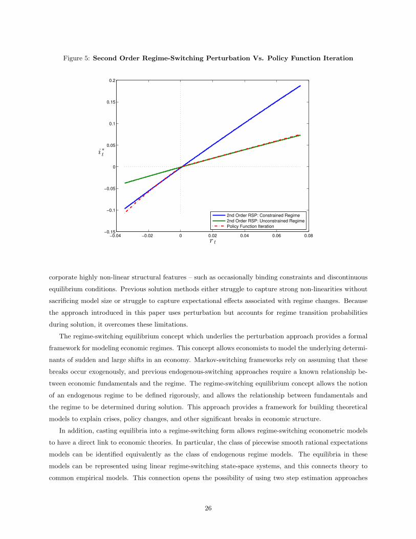
Figure 5: Second Order Regime-Switching Perturbation Vs. Policy Function Iteration

−0.04 −0.02 0 0.02 0.04 0.06 0.08−0.15

−0.1

−0.05

0

0.05

0.1

0.15

0.2

i∗

t

r t

2nd Order RSP: Constrained Regime

2nd Order RSP: Unconstrained Regime

Policy Function Iteration

corporate highly non-linear structural features – such as occasionally binding constraints and discontinuous

equilibrium conditions. Previous solution methods either struggle to capture strong non-linearities without

sacrificing model size or struggle to capture expectational effects associated with regime changes. Because

the approach introduced in this paper uses perturbation but accounts for regime transition probabilities

during solution, it overcomes these limitations.

The regime-switching equilibrium concept which underlies the perturbation approach provides a formal

framework for modeling economic regimes. This concept allows economists to model the underlying determi-

nants of sudden and large shifts in an economy. Markov-switching frameworks rely on assuming that these

breaks occur exogenously, and previous endogenous-switching approaches require a known relationship be-

tween economic fundamentals and the regime. The regime-switching equilibrium concept allows the notion

of an endogenous regime to be defined rigorously, and allows the relationship between fundamentals and

the regime to be determined during solution. This approach provides a framework for building theoretical

models to explain crises, policy changes, and other significant breaks in economic structure.

In addition, casting equilibria into a regime-switching form allows regime-switching econometric models

to have a direct link to economic theories. In particular, the class of piecewise smooth rational expectations

models can be identified equivalently as the class of endogenous regime models. The equilibria in these

models can be represented using linear regime-switching state-space systems, and this connects theory to

common empirical models. This connection opens the possibility of using two step estimation approaches

26

based on reduced-form regime-switching econometric models to estimate highly non-linear DSGE models.

Future work will:

1. Estimate the model of Gust et al. (2012) using regime-switching perturbation and filtering based on

the resulting linear regime switching state space system. This exercise will demonstrate how estimation

based on this solution technique compares to estimation based on the solutions generated by global

methods.

2. Demonstrate how the method scales with state-space dimension by solving an N -country global econ-

omy model of sudden stops based on Korinek and Mendoza (2013). In the model, each country has two

continuous state variables and a subset of countries have occasionally binding collateral constraints. In

this extension of the canonical sudden stop framework, the global risk-free rate is endogenously deter-

mined from global financial conditions. The model has 2N state variables so increasing the number of

countries will reveal the scaling properties of the technique. This numerical exercise will directly show

how leveraging perturbation breaks the curse of dimensionality and allows the study of very large and

very non-linear models.

3. Illustrate how to use this technique to study extreme equilibrium dynamics and large shocks. Because

the method uses reference points for perturbation that can be chosen ex-ante, the solution does not

need to remain close to a single steady state. Solution functions can be approximated local to many

points in the space of outcomes.

4. Develop and apply a joint solution and estimation procedure in the spirit of Imai et al. (2009) and

examine two-step estimation using regime-switching reduced-form models.

5. Apply these tools to (a) study unconventional monetary policy at the zero-lower-bound, (b) model

international capital markets in the presence of endogenous global financial crises, (c) model trade

specialization dynamics, and (d) model asymmetric business cycles.

27

References

K. Adam and M. Grill. Optimal sovereign default. Discussion Papers 09/2013, Deutsche Bundesbank,

Research Centre, 2013. URL http://ideas.repec.org/p/zbw/bubdps/092013.html.

S. Adjemian, H. Bastani, F. Karame, M. Juillard, J. Maih, F. Mihoubi, G. Perendia, J. Pfeifer, M. Ratto,

and S. Villemot. Dynare: Reference manual version 4. Technical report, CEPREMAP, 2014.

C. Arellano. Default risk and income fluctuations in emerging economies. American Economic Review, 98(3):

690–712, 2008. doi: 10.1257/aer.98.3.690. URL http://www.aeaweb.org/articles.php?doi=10.1257/

aer.98.3.690.

S. B. Aruoba and F. Schorfheide. Macroeconomic dynamics near the zlb: A tale of two equilibria. Technical

report, 2012.

J. Barthelemy and M. Marx. State-Dependent Probability Distributions in Non Linear Rational Expectations

Models. Technical report, 2013.

F. Bianchi. Evolving monetary/fiscal policy mix in the united states. The American Economic Review, 102

(3):167–172, 2012.

F. Bianchi. Regime switches, agents’ beliefs, and post-world war ii us macroeconomic dynamics. The Review

of Economic Studies, 80(2):463–490, 2013.

F. Bianchi and L. Melosi. Modeling the evolution of expectations and uncertainty in general equilibrium.

Technical report, Penn Institute for Economic Research, Department of Economics, University of Penn-

sylvania, 2012.

J. Bianchi and E. G. Mendoza. Optimal time-consistent macroprudential policy. NBER Working Papers

19704, National Bureau of Economic Research, Inc, Dec 2013. URL http://ideas.repec.org/p/nbr/

nberwo/19704.html.

F. Boissay, F. Collard, and F. Smets. Booms and banking crises. Technical report, Working Paper, 2013.

R. A. Braun, L. M. Korber, and Y. Waki. Some unpleasant properties of log-linearized solutions when the

nominal rate is zero. Technical report, 2012.

M. Brzoza-Brzezina, M. Kolasa, and K. Makarski. A penalty function approach to occasionally binding

credit constraints. Dynare Working Papers 27, CEPREMAP, June 2013. URL http://ideas.repec.

org/p/cpm/dynare/027.html.

S. Cho. Characterizing markov-switching rational expectations models. Technical report, 2013. URL F.

S. Cho and A. Moreno. The Forward Solution for Linear Rational Expectations Models. Technical report,

2008.

28

T. Davig and E. M. Leeper. Endogenous monetary policy regime change. NBER Working Papers 12405,

National Bureau of Economic Research, Inc, Aug. 2006. URL http://ideas.repec.org/p/nbr/nberwo/

12405.html.

P. Dreesen, K. Batselier, and B. De Moor. Back to the roots: Polynomial system solving, linear algebra,

systems theory. Proc 16th IFAC Symposium on System Identification (SYSID 2012), pages 1203–1208,

2012.

R. Farmer and V. Khramov. Solving and Estimating Indeterminate DSGE Models. IMF Working Pa-

pers 13/200, International Monetary Fund, Oct. 2013. URL http://ideas.repec.org/p/imf/imfwpa/

13-200.html.

R. E. Farmer, D. F. Waggoner, and T. Zha. Understanding markov-switching rational expectations models.

Journal of Economic Theory, 144(5):1849–1867, 2009.

R. E. Farmer, D. F. Waggoner, and T. Zha. Minimal state variable solutions to markov-switching rational

expectations models. Journal of Economic Dynamics and Control, 35(12):2150–2166, 2011.

J. Fernandez-Villaverde, G. Gordon, P. A. Guerron-Quintana, and J. Rubio-Ramirez. Nonlinear adventures

at the zero lower bound. Working Paper 18058, National Bureau of Economic Research, May 2012. URL

http://www.nber.org/papers/w18058.

A. Foerster, J. Rubio-Ramirez, D. Waggoner, and T. Zha. Perturbation methods for markov-switching dsge

model. Technical report, 2013.

A. T. Foerster. Monetary policy regime switches and macroeconomic dynamic. Technical report, 2013.

W. T. Gavin, B. D. Keen, A. Richter, and N. Throckmorton. Global dynamics at the zero lower bound.

Federal Reserve Bank of St. Louis Working Paper Series, (2013-007), 2013.

M. Gertler and N. Kiyotaki. Banking, liquidity and bank runs in an infinite horizon economy. 2013 Meeting

Papers 59, Society for Economic Dynamics, 2013. URL http://ideas.repec.org/p/red/sed013/59.

html.

L. Guerrieri and M. Iacoviello. Occbin: A toolkit for solving dynamic models with occasionally binding

constraints easily, 2014.

C. Gust, J. D. Lopez-Salido, and M. E. Smith. The empirical implications of the interest-rate lower bound.

Technical report, CEPR Discussion Papers, 2012.

Z. He and A. Krishnamurthy. A macroeconomic framework for quantifying systemic risk. Working Paper

Research 233, National Bank of Belgium, Oct 2012. URL http://ideas.repec.org/p/nbb/reswpp/

201210-233.html.

29

Z. He and A. Krishnamurthy. Intermediary asset pricing. American Economic Review, 103(2):732–70,

2013. doi: 10.1257/aer.103.2.732. URL http://www.aeaweb.org/articles.php?doi=10.1257/aer.103.

2.732.

S. Imai, N. Jain, and A. Ching. Bayesian estimation of dynamic discrete choice models. Econometrica, 77

(6):pp. 1865–1899, 2009. ISSN 00129682. URL http://www.jstor.org/stable/25621385.

H. Jin and K. L. Judd. Perturbation methods for general dynamic stochastic models. Manuscript, Stanford

University, 2002.

J. Kim, S. Kim, E. Schaumburg, and C. A. Sims. Calculating and using second-order accurate solutions

of discrete time dynamic equilibrium models. Journal of Economic Dynamics and Control, 32(11):3397

– 3414, 2008. ISSN 0165-1889. doi: http://dx.doi.org/10.1016/j.jedc.2008.02.003. URL http://www.

sciencedirect.com/science/article/pii/S0165188908000316.

A. Korinek and E. G. Mendoza. From sudden stops to fisherian deflation: Quantitative theory and policy

implications. NBER Working Papers 19362, National Bureau of Economic Research, Inc, Aug. 2013. URL

http://ideas.repec.org/p/nbr/nberwo/19362.html.

T. A. Lubik and F. Schorfheide. Computing sunspot equilibria in linear rational expectations models. Journal

of Economic Dynamics and Control, 28(2):273–285, November 2003. URL http://ideas.repec.org/a/

eee/dyncon/v28y2003i2p273-285.html.

E. G. Mendoza. Sudden stops, financial crises, and leverage. American Economic Review, 100(5):1941–

66, 2010. doi: 10.1257/aer.100.5.1941. URL http://www.aeaweb.org/articles.php?doi=10.1257/aer.

100.5.1941.

E. G. Mendoza and K. A. Smith. Quantitative implications of a debt-deflation theory of sudden stops and

asset prices. Journal of International Economics, 70(1):82 – 114, 2006. ISSN 0022-1996. doi: http:

//dx.doi.org/10.1016/j.jinteco.2005.06.016. URL http://www.sciencedirect.com/science/article/

pii/S002219960500098X.

E. G. Mendoza and V. Z. Yue. A general equilibrium model of sovereign default and business cycles. The

Quarterly Journal of Economics, 127(2):889–946, 2012. URL http://ideas.repec.org/a/oup/qjecon/

v127y2012i2p889-946.html.

T. Nakata. Optimal fiscal and monetary policy with occasionally binding zero bound constraints. Technical

report, 2012.

Y. Sannikov and M. Brunnermeier. A macroeconomic model with a financial sector. 2012 Meeting Papers

507, Society for Economic Dynamics, 2012. URL http://ideas.repec.org/p/red/sed012/507.html.

Y. Sannikov and M. Brunnermeier. The i-theory of money. 2013 Meeting Papers 620, Society for Economic

Dynamics, 2013. URL http://ideas.repec.org/p/red/sed013/620.html.

30

S. Schmitt-Grohe and M. Uribe. Solving dynamic general equilibrium models using a second-order approxi-

mation to the policy function. Journal of Economic Dynamics and Control, 28(4):755–775, January 2004.

URL http://ideas.repec.org/a/eee/dyncon/v28y2004i4p755-775.html.

31

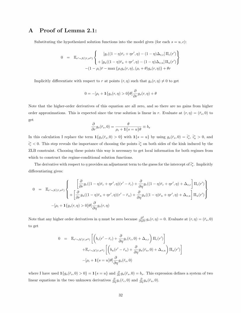
A Proof of Lemma 2.1:

Substituting the hypothesized solution functions into the model gives (for each s = u, c):

0 = Er′∼N (r,σ2)

[gc((1− η)rc + ηr′, η)− (1− η)∆s,c] Πc(r′)

+ [gu((1− η)ru + ηr′, η)− (1− η)∆s,u] Πu(r′)

−(1− ρi)r −max {ρigs(r, η), (ρi + θ)gs(r, η)}+ θr

Implicitly differentiate with respect to r at points (r, η) such that gs(r, η) 6= 0 to get

0 = −[ρi + 1{gs(r, η) > 0}θ] ∂∂rgs(r, η) + θ

Note that the higher-order derivatives of this equation are all zero, and so there are no gains from higher

order approximations. This is expected since the true solution is linear in r. Evaluate at (r, η) = (rs, 0) to

get∂

∂rgs(rs, 0) =

θ

ρi + 1{s = u}θ≡ bs

In this calculation I replace the term 1{gs(rs, 0) > 0} with 1{s = u} by using gs(rs, 0) = i∗s, i∗u > 0, and

i∗c < 0. This step reveals the importance of choosing the points i∗s on both sides of the kink induced by the

ZLB constraint. Choosing these points this way is necessary to get local information for both regimes from

which to construct the regime-conditional solution functions.

The derivative with respect to η provides an adjustment term to the guess for the intercept of i∗s. Implicitly

differentiating gives:

0 = Er′∼N (r,σ2)

[∂

∂rgc((1− η)rc + ηr′, η)(r′ − rc) +

∂

∂ηgc((1− η)rc + ηr′, η) + ∆s,c

]Πc(r

′)

+

[∂

∂rgu((1− η)ru + ηr′, η)(r′ − ru) +

∂

∂ηgu((1− η)ru + ηr′, η) + ∆s,u

]Πu(r′)

−[ρi + 1{gs(r, η) > 0}θ] ∂

∂ηgs(r, η)

Note that any higher order derivatives in η must be zero because ∂2

∂η∂rgs(r, η) = 0. Evaluate at (r, η) = (rs, 0)

to get

0 = Er′∼N (r,σ2)

[(bc(r

′ − rc) +∂

∂ηgc(rc, 0) + ∆s,c

)Πc(r

′)

]+Er′∼N (r,σ2)

[(bu(r′ − ru) +

∂

∂ηgu(ru, 0) + ∆s,u

)Πu(r′)

]−[ρi + 1{s = u}θ] ∂

∂ηgs(rs, 0)

where I have used 1{gs(rs, 0) > 0} = 1{s = u} and ∂∂rgs(rs, 0) = bs. This expression defines a system of two

linear equations in the two unknown derivatives ∂∂η gc(rc, 0) and ∂

∂η gu(ru, 0).

32

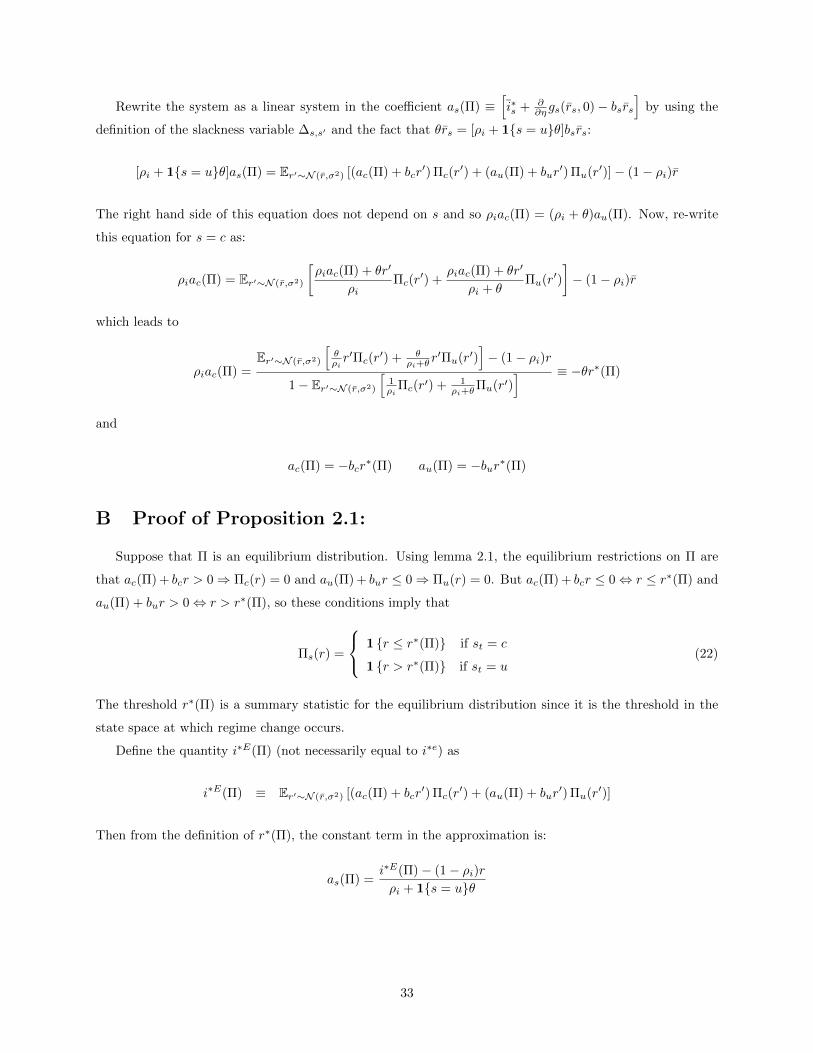
Rewrite the system as a linear system in the coefficient as(Π) ≡[i∗s + ∂

∂η gs(rs, 0)− bsrs]

by using the

definition of the slackness variable ∆s,s′ and the fact that θrs = [ρi + 1{s = u}θ]bsrs:

[ρi + 1{s = u}θ]as(Π) = Er′∼N (r,σ2) [(ac(Π) + bcr′) Πc(r

′) + (au(Π) + bur′) Πu(r′)]− (1− ρi)r

The right hand side of this equation does not depend on s and so ρiac(Π) = (ρi + θ)au(Π). Now, re-write

this equation for s = c as:

ρiac(Π) = Er′∼N (r,σ2)

[ρiac(Π) + θr′

ρiΠc(r

′) +ρiac(Π) + θr′

ρi + θΠu(r′)

]− (1− ρi)r

which leads to

ρiac(Π) =Er′∼N (r,σ2)

[θρir′Πc(r

′) + θρi+θ

r′Πu(r′)]− (1− ρi)r

1− Er′∼N (r,σ2)

[1ρi

Πc(r′) + 1ρi+θ

Πu(r′)] ≡ −θr∗(Π)

and

ac(Π) = −bcr∗(Π) au(Π) = −bur∗(Π)

B Proof of Proposition 2.1:

Suppose that Π is an equilibrium distribution. Using lemma 2.1, the equilibrium restrictions on Π are

that ac(Π) + bcr > 0⇒ Πc(r) = 0 and au(Π) + bur ≤ 0⇒ Πu(r) = 0. But ac(Π) + bcr ≤ 0⇔ r ≤ r∗(Π) and

au(Π) + bur > 0⇔ r > r∗(Π), so these conditions imply that

Πs(r) =

1 {r ≤ r∗(Π)} if st = c

1 {r > r∗(Π)} if st = u(22)

The threshold r∗(Π) is a summary statistic for the equilibrium distribution since it is the threshold in the

state space at which regime change occurs.

Define the quantity i∗E(Π) (not necessarily equal to i∗e) as

i∗E(Π) ≡ Er′∼N (r,σ2) [(ac(Π) + bcr′) Πc(r

′) + (au(Π) + bur′) Πu(r′)]

Then from the definition of r∗(Π), the constant term in the approximation is:

as(Π) =i∗E(Π)− (1− ρi)rρi + 1{s = u}θ

33

Substitute the terms ac(Π) and au(Π) into the definition of i∗E(Π) to get:

i∗E(Π) =

∫[(ac(Π) + bcr

′) Πc(r′) + (au(Π) + bur

′) Πu(r′)]1

σφ

(r′ − rσ

)dr′

=

∫ [i∗E(Π)− (1− ρi)r + θr′

ρiΠc(r

′) +i∗E(Π)− (1− ρi)r + θr′

ρi + θΠu(r′)

]1

σφ

(r′ − rσ

)dr′

=

∫max

{i∗E(Π)− (1− ρi)r + θr′

ρi,i∗E(Π)− (1− ρi)r + θr′

ρi + θ

}1

σφ

(r′ − rσ

)dr′

where the last line follows since Π is an equilibrium distribution and must be of the form (22). This condition

is the same fixed point condition in (4). Therefore i∗E(Π) = i∗e where i∗e is some solution of condition (4).

Therefore, the constant terms must be identical to the constant terms in the true solution.

C Proof of Proposition 2.2:

The update equation (12) implies that after a single iteration of the algorithm, the threshold r∗(Π(n−1))

is a sufficient statistic for the distribution Π(n). In particular:

Π(n)s (r) =

1{r ≤ r∗(Π(n−1))

}if s = c

1{r > r∗(Π(n−1))

}if s = u

This recursion can be re-expressed as a recursive condition on the threshold using the definition of r∗:

r∗(Π(n)) =(1− ρi)r −

∫ [Π

(n)c

θρi

(r′ − r∗(Π(n))) + Π(n)u

θρi+θ

(r′ − r∗(Π(n)))]

1σφ(r′−rσ

)dr′

θ

=(1− ρi)r

θ−∫

max

{1

ρi(r′ − r∗(Π(n−1))),

1

ρi + θ(r′ − r∗(Π(n−1)))

}1

σφ

(r′ − rσ

)dr′

−Φ

(r∗(Π(n−1))− r

σ

)1

ρi[r∗(Π(n−1))− r∗(Π(n))]

−

[1− Φ

(r∗(Π(n−1))− r

σ

)]1

ρi + θ[r∗(Π(n−1))− r∗(Π(n))]

where Φ is the cdf of the standard normal distribution. Let r∗n ≡ r∗(Π(n)). This threshold update equation

can be written as:

r∗n = r∗n−1 +

(1−ρi)rθ +

∫max

{1−ρiρi

r∗n−1 − 1ρir′, 1−ρi−θ

ρi+θr∗n−1 − 1

ρi+θr′}

1σφ(r′−rσ

)dr′

1−{

Φ(r∗n−1−r

σ

)1ρi

+[1− Φ

(r∗n−1−r

σ

)]1

ρi+θ

} ≡ m(r∗n−1) (23)

The mapm is continuously differentiable everywhere except for a single singularity at the point σΦ−1(ρi(1−ρi−θ)

θ

).

Moreover, it is strictly decreasing every except at this singularity. There are then precisely two points r∗ such

that r∗ = m(r∗). For sufficiently small σ, both of these points are dynamically stable. Therefore r∗n → r∗

for one of these two points.

34

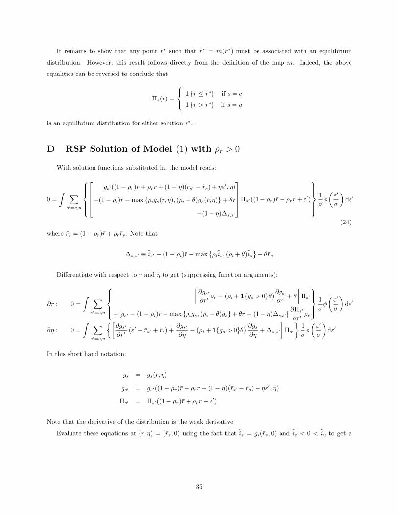
It remains to show that any point r∗ such that r∗ = m(r∗) must be associated with an equilibrium

distribution. However, this result follows directly from the definition of the map m. Indeed, the above

equalities can be reversed to conclude that

Πs(r) =

1 {r ≤ r∗} if s = c

1 {r > r∗} if s = u

is an equilibrium distribution for either solution r∗.

D RSP Solution of Model (1) with ρr > 0

With solution functions substituted in, the model reads:

0 =

∫ ∑s′=c,u

gs′((1− ρr)r + ρrr + (1− η)(rs′ − rs) + ηε′, η)

−(1− ρi)r −max {ρigs(r, η), (ρi + θ)gs(r, η)}+ θr

−(1− η)∆s,s′

Πs′((1− ρr)r + ρrr + ε′)

1

σφ

(ε′

σ

)dε′

(24)

where rs = (1− ρr)r + ρr rs. Note that

∆s,s′ ≡ is′ − (1− ρi)r −max{ρiis, (ρi + θ)is

}+ θrs

Differentiate with respect to r and η to get (suppressing function arguments):

∂r : 0 =

∫ ∑s′=c,u

[∂gs′

∂r′ρr − (ρi + 1{gs > 0}θ)∂gs

∂r+ θ

]Πs′

+ [gs′ − (1− ρi)r −max {ρigs, (ρi + θ)gs}+ θr − (1− η)∆s,s′ ]∂Πs′

∂r′ρr

1

σφ

(ε′

σ

)dε′

∂η : 0 =

∫ ∑s′=c,u

{[∂gs′

∂r′(ε′ − rs′ + rs) +

∂gs′

∂η− (ρi + 1{gs > 0}θ) ∂gs

∂η+ ∆s,s′

]Πs′

}1

σφ

(ε′

σ

)dε′

In this short hand notation:

gs = gs(r, η)

gs′ = gs′((1− ρr)r + ρrr + (1− η)(rs′ − rs) + ηε′, η)

Πs′ = Πs′((1− ρr)r + ρrr + ε′)

Note that the derivative of the distribution is the weak derivative.

Evaluate these equations at (r, η) = (rs, 0) using the fact that is = gs(rs, 0) and ic < 0 < iu to get a

35

system of linear equations in the unknown derivatives:

0 =∑s′=c,u

G(1,0)s′ ρrΠs,s′ + θ − (ρi + 1{s = u}θ)G(1,0)

s

0 =

∫ ∑s′=c,u

[G

(1,0)s′ µ

(1)s,s′ +G

(0,1)s′ + ∆s,s′

]Πs,s′ − (ρi + 1{s = u}θ)G(0,1)

s

with the notation:

G(i,j)s ≡ ∂i+jgs(r, η)

∂ri∂ηj

∣∣∣∣(r,η)=(rs,0)

µ(i)s,s′ ≡

∫(ε′ − rs′ + rs)

iΠs′(rs + ε′)σ−1φ(ε′/σ)dε′∫

Πs′(rs + ε′)σ−1φ(ε′/σ)dε′

Πs,s′ ≡∫

Πs′(rs + ε′)σ−1φ(ε′/σ)dε′

To get this expression, note that the term gs′− (1−ρi)r−max {ρigs, (ρi + θ)gs}+θr− (1−η)∆s,s′ evaluates

to zero by the construction of ∆s,s′ . The solution of this system gives the first order approximation:

gs(r, η) ≈ is +G(1,0)s (r − rs) +G(0,1)

s η

Next, take the second order derivatives of (24):

∂r2 : 0 =

∫ ∑s′=c,u

[∂2gs′

∂r′2ρ2r − (ρi + 1{gs > 0}θ)∂

2gs∂r2

]Πs′

+2

[∂gs′

∂r′ρr − (ρi + 1{gs > 0}θ)∂gs

∂r+ θ

]∂Πs′

∂r′ρr

+ [gs′ − (1− ρi)r −max {ρigs, (ρi + θ)gs}+ θr − (1− η)∆s,s′ ]∂2Πs′

∂r′2ρ2r

1

σφ

(ε′

σ

)dε′

∂η2 : 0 =

∫ ∑s′=c,u

∂2gs′

∂r′2(ε′ − rs′ + rs)

2+ 2

∂gs′

∂r′∂η(ε′ − rs′ + rs) +

∂2gs′

∂η2

− (ρi + 1{gs > 0}θ) ∂2gs∂η2

Πs′

1

σφ

(ε′

σ

)dε′

∂r∂η : 0 =

∫ ∑s′=c,u

[∂2gs′

∂r′2ρr (ε′ − rs′ + rs) +

∂2gs′

∂r′∂ηρr − (ρi + 1{gs > 0}θ) ∂

2gs∂r∂η

]Πs′

+

[∂gs′

∂r′(ε′ − rs′ + rs) +

∂gs′

∂η− (ρi + 1{gs > 0}θ) ∂gs

∂η+ ∆s,s′

]∂Πs′

∂r′ρr

1

σφ

(ε′

σ

)dε′

Evaluate at (r, η) = (rs, 0) to get a another linear system of equations in the second order derivatives given

36

the first order derivatives

0 =∑s′=c,u

[G

(2,0)s′ ρ2

r − (ρi + 1{gs > 0}θ)G(2,0)s

]Πs,s′

+2[G

(1,0)s′ ρr − (ρi + 1{gs > 0}θ)G(1,0)

s + θ]

Π(1)s,s′ρr

0 =

∫ ∑s′=c,u

G(2,0)

s′ µ(2)s,s′ + 2G

(1,1)s′ µ

(1)s,s′ +G

(0,2)s′

− (ρi + 1{gs > 0}θ)G(0,2)s

Πs,s′

0 =

∫ ∑s′=c,u

[G

(2,0)s′ ρrµ

(1)s,s′ +G

(1,1)s′ ρr − (ρi + 1{gs > 0}θ)G(1,1)

s

]Πs,s′

+[G

(1,0)s′ µ

(1/1)s,s′ +G

(0,1)s′ − (ρi + 1{gs > 0}θ)G(0,1)

s + ∆s,s′

]Π

(1)s,s′ρr

where now

µ(i/j)s,s′ ≡

∫(ε′ − rs′ + rs)

i ∂jΠs′ (rs+ε′)∂r′j

σ−1φ(ε′/σ)dε′∫ ∂jΠs′ (rs+ε′)∂r′j

σ−1φ(ε′/σ)dε′=

∫(ε′ − rs′ + rs)

iΠs′(rs + ε′)σ−1−jφ(j)(ε′/σ)dε′∫

Πs′(rs + ε′)σ−1−jφ(j)(ε′/σ)dε′

Π(i)s,s′ ≡

∫Πs′(rs + ε′)σ−1−jφ(j)(ε′/σ)dε′

where φ(j) denotes the j-th derivative of the standard normal pdf and the second equality in both lines

follows from the definition of the weak derivative.

Solving for these second order derivatives leads to the second order Taylor approximation:

gs(r, η) ≈ is +G(1,0)s (r − rs) +G(0,1)

s η

+1

2G(2,0)s (r − rs)2 +G(1,1)

s (r − rs)η +1

2G(0,2)s η2

E Exogenous and Threshold Regime-Switching as a Special Case

To construct a Markov-switching model, factor the control vector as Yt = (Y 0t , Y

st ) where Y st = st denotes

the present regime. Then let one of the state variables keep track of the past regime, so factor the state

vector in a similar way as Xt = (X0t , X

st ) and include an equation which specifies that the next period value

of this state variable is the current value of the regime: Xst+1 = Y st . Assume that there is a component

of the exogenous shock vector υt which (in-equilibrium) governs the regime given the past regime (which is

equal to the value of Xst ). Partition the shocks as: εt = (ε0

t , υt). Assume that υt = (υ1t , . . . , υ

St ) with υst an

IID extreme value type 1 random variable. Let {βs,s′}Ss,s′=1 be coefficients which will control the switching

probabilities and specify the present regime as:

Xst+1 = Y st = st =

S∑r=1

s1{s = arg max

s[βs0,s1 {Xs

t ∈ Rs0}+ υst ]}

(25)

Here {Rs}NSs=1 defines a partition of R so that for each s = 1, . . . , S the integer s is in the interior of Rs. As

a result, the equation is well defined on the entire real line for any Xst ∈ R. Moreover, the equilibrium value

37

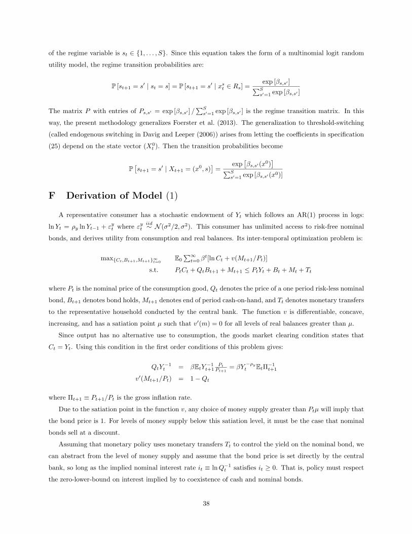
of the regime variable is st ∈ {1, . . . , S}. Since this equation takes the form of a multinomial logit random

utility model, the regime transition probabilities are:

P [st+1 = s′ | st = s] = P [st+1 = s′ | xst ∈ Rs] =exp [βs,s′ ]∑Ss′=1 exp [βs,s′ ]

The matrix P with entries of Ps,s′ = exp [βs,s′ ] /∑Ss′=1 exp [βs,s′ ] is the regime transition matrix. In this

way, the present methodology generalizes Foerster et al. (2013). The generalization to threshold-switching

(called endogenous switching in Davig and Leeper (2006)) arises from letting the coefficients in specification

(25) depend on the state vector (X0t ). Then the transition probabilities become

P[st+1 = s′ | Xt+1 = (x0, s)

]=

exp[βs,s′(x

0)]∑S

s′=1 exp [βs,s′(x0)]

F Derivation of Model (1)

A representative consumer has a stochastic endowment of Yt which follows an AR(1) process in logs:

lnYt = ρy lnYt−1 + εyt where εytiid∼ N (σ2/2, σ2). This consumer has unlimited access to risk-free nominal

bonds, and derives utility from consumption and real balances. Its inter-temporal optimization problem is:

max{Ct,Bt+1,Mt+1}∞t=0E0

∑∞t=0 β

t[lnCt + v(Mt+1/Pt)]

s.t. PtCt +QtBt+1 +Mt+1 ≤ PtYt +Bt +Mt + Tt

where Pt is the nominal price of the consumption good, Qt denotes the price of a one period risk-less nominal

bond, Bt+1 denotes bond holds, Mt+1 denotes end of period cash-on-hand, and Tt denotes monetary transfers

to the representative household conducted by the central bank. The function v is differentiable, concave,

increasing, and has a satiation point µ such that v′(m) = 0 for all levels of real balances greater than µ.

Since output has no alternative use to consumption, the goods market clearing condition states that

Ct = Yt. Using this condition in the first order conditions of this problem gives:

QtY−1t = βEtY −1

t+1Pt

Pt+1= βY

−ρyt EtΠ−1

t+1

v′(Mt+1/Pt) = 1−Qt

where Πt+1 ≡ Pt+1/Pt is the gross inflation rate.

Due to the satiation point in the function v, any choice of money supply greater than Ptµ will imply that

the bond price is 1. For levels of money supply below this satiation level, it must be the case that nominal

bonds sell at a discount.

Assuming that monetary policy uses monetary transfers Tt to control the yield on the nominal bond, we

can abstract from the level of money supply and assume that the bond price is set directly by the central

bank, so long as the implied nominal interest rate it ≡ lnQ−1t satisfies it ≥ 0. That is, policy must respect

the zero-lower-bound on interest implied by to coexistence of cash and nominal bonds.

38

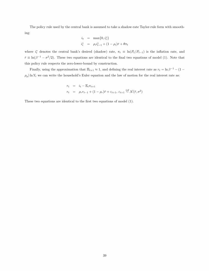
The policy rule used by the central bank is assumed to take a shadow-rate Taylor-rule form with smooth-

ing:

it = max{0, i∗t }

i∗t = ρii∗t−1 + (1− ρi)r + θπt

where i∗t denotes the central bank’s desired (shadow) rate, πt ≡ ln(Pt/Pt−1) is the inflation rate, and

r ≡ ln(β−1 − σ2/2). These two equations are identical to the final two equations of model (1). Note that

this policy rule respects the zero-lower-bound by construction.

Finally, using the approximation that Πt+1 ≈ 1, and defining the real interest rate as rt = lnβ−1 − (1−

ρy) lnYt we can write the household’s Euler equation and the law of motion for the real interest rate as:

rt = it − Etπt+1

rt = ρrrt−1 + (1− ρr)r + εt+1, εt+1iid∼ N (r, σ2)

These two equations are identical to the first two equations of model (1).

39