experiments with remote entanglement using single … · wave in a solid state medium di racts ......
TRANSCRIPT

Experiments with remote entanglement using single barium ions
Nathan Kurz
A dissertationsubmitted in partial fulfillment of the
requirements for the degree of
Doctor of Philosophy
University of Washington
2010
Program authorized to offer degree:Physics

University of WashingtonGraduate School
This is to certify that I have examined this copy of a doctoral dissertationby
Nathan Kurz
and have found it complete and satisfactory in all respects,and that any and all revisions required by the final
examining committee have been made.
Chair of the Supervisory Committee:
Boris B. Blinov
Reading Committee:
Boris B. Blinov
Larry Sorensen
David Cobden
Date:

In presenting this dissertation in partial fulfillment of the requirementsfor the doctoral degree at the University of Washington, I agree that the Li-brary shall make its copies freely available for inspection. I further agree thatextensive copying of the dissertation is allowable only for scholarly purposes,consistent with“fair us” as prescribed in the U.S. Copyright Law. Requestsfor copying or reproduction of this dissertation may be referred to ProQuestInformation and Learning, 300 North Zeeb Road, Ann Arbor, MI 48106-1346,1-800-521-0600, to whom the author has granted “the right to reproduce andsell (a) copies of the manuscript in microform and/or (b) printed copies ofthe manuscript made from microform.”
Signature
Date

University of Washington
Abstract
Experiments with remote entanglement using single barium ions
Nathan Kurz
Chair of the Supervisory Committee:Dr. Boris B. BlinovPhysics Department
Barium ion qubits are trapped and Doppler cooled in a linear Paul trap and
the tasks of state initialization, single-qubit operations and detection are
demonstrated. Coherent qubit excitation us accomplished on the 6S1/2 ↔
6P3/2 and the 6S1/2 ↔ 6P1/2 transitions are single pulses from a mode-locked
Ti:Sapphire laser, with the eventual goal of entangling the polarization mode
of emitted photons with the spin state of the ion. Single photon generation
and detection ability is demonstrated. A stabilized 1.762 µm laser is used
on the 6S1/2 → 5D5/2 transition to demonstrate the ability to state selec-
tively shelve the ion from the ground state to be used as readout. Using the
techniques that enable qubit operations and readout, several quantities of
interest in 138Ba+ are measured either for the first time or to higher accuracy
than previously achieved.

TABLE OF CONTENTS
Page
List of Figures . . . . . . . . . . . . . . . . . . . . . . . . . . . . . . . . . . . . . . . . . . . . . . . . . . . . . . . . . . . ii
List of Tables . . . . . . . . . . . . . . . . . . . . . . . . . . . . . . . . . . . . . . . . . . . . . . . . . . . . . . . . . . . iii
Abbreviations . . . . . . . . . . . . . . . . . . . . . . . . . . . . . . . . . . . . . . . . . . . . . . . . . . . . . . . . . . . iv
Chapter I: Atomic Physics & Quantum Computation . . . . . . . . . . . . . . . . . . . . . 1
1.1 Introduction . . . . . . . . . . . . . . . . . . . . . . . . . . . . . . . . . . . . . . . . . . . . . . . . . . . 1
1.2 Atom-light interactions . . . . . . . . . . . . . . . . . . . . . . . . . . . . . . . . . . . . . . . . . 5
1.3 Matrix elements & multipole expansion . . . . . . . . . . . . . . . . . . . . . . . 11
Chapter II: Ion Traps & Lasers . . . . . . . . . . . . . . . . . . . . . . . . . . . . . . . . . . . . . . . . . .19
2.1 Ion trapping . . . . . . . . . . . . . . . . . . . . . . . . . . . . . . . . . . . . . . . . . . . . . . . . . . 19
2.2 Doppler cooling - a semiclassical picture . . . . . . . . . . . . . . . . . . . . . . . 23
2.3 Doppler cooling - a quantum perspective . . . . . . . . . . . . . . . . . . . . . . 25
2.4 Trapping and cooling Ba+ . . . . . . . . . . . . . . . . . . . . . . . . . . . . . . . . . . . . .27
Chapter III: Ultrafast interactions . . . . . . . . . . . . . . . . . . . . . . . . . . . . . . . . . . . . . . . 41
3.1 Mode-locked lasers . . . . . . . . . . . . . . . . . . . . . . . . . . . . . . . . . . . . . . . . . . . 42
3.2 Ultrafast pulses & ions . . . . . . . . . . . . . . . . . . . . . . . . . . . . . . . . . . . . . . . 45
3.3 Single pulse selection . . . . . . . . . . . . . . . . . . . . . . . . . . . . . . . . . . . . . . . . . 46
3.4 Rabi flop at 455 nm . . . . . . . . . . . . . . . . . . . . . . . . . . . . . . . . . . . . . . . . . . 48
3.5 Branching ratios from 6P3/2 . . . . . . . . . . . . . . . . . . . . . . . . . . . . . . . . . . 50
3.6 Ultrafast excitation at 493 nm . . . . . . . . . . . . . . . . . . . . . . . . . . . . . . . . 56
Chapter IV: Single Photon Source . . . . . . . . . . . . . . . . . . . . . . . . . . . . . . . . . . . . . . 61
i
4.1 Single photon interference on a beam splitter . . . . . . . . . . . . . . . . . 62
4.2 Experimental verification of single photon generation . . . . . . . . . 67
Chapter V: Initialization & Readout . . . . . . . . . . . . . . . . . . . . . . . . . . . . . . . . . . . .71
5.1 Magnetic field effects, briefly . . . . . . . . . . . . . . . . . . . . . . . . . . . . . . . . . 71
5.2 Optical pumping . . . . . . . . . . . . . . . . . . . . . . . . . . . . . . . . . . . . . . . . . . . . . 76
5.3 Shelving to 5D5/2 at 1.762 µm . . . . . . . . . . . . . . . . . . . . . . . . . . . . . . . . 79
5.4 Precise measurement of g5D5/2. . . . . . . . . . . . . . . . . . . . . . . . . . . . . . . . 82
Chapter VI: Toward a Zeeman qubit & outlook . . . . . . . . . . . . . . . . . . . . . . . . . 91
6.1 Zeeman qubit: How & why? . . . . . . . . . . . . . . . . . . . . . . . . . . . . . . . . . .92
6.2 From entangled ions and photons to entangled ions . . . . . . . . . . . 95
6.3 Applications . . . . . . . . . . . . . . . . . . . . . . . . . . . . . . . . . . . . . . . . . . . . . . . . . .98
Bibliography . . . . . . . . . . . . . . . . . . . . . . . . . . . . . . . . . . . . . . . . . . . . . . . . . . . . . . . . . . . 103
ii

LIST OF FIGURES
Figure Number Page
1.1 Bloch sphere representation of a general qubit state . . . . . . . . . . . . . . . . . . . 5
1.2 Rabi oscillations, on resonance and detuned. . . . . . . . . . . . . . . . . . . . . . . . . . .9
1.3 Lamba structure with Rabi frequencies, detunings and decay rates . . . 11
1.4 Multipole radiation patterns (a) dipole, (b) quadrupole . . . . . . . . . . . . . . 12
1.5 Relative intensities for transitions in an I = 3/2 ion . . . . . . . . . . . . . . . . . 17
2.1 Secular motion and micromotion of an ion in a Paul trap . . . . . . . . . . . . 22
2.2 Not-to-scale drawing of a linear Paul trap . . . . . . . . . . . . . . . . . . . . . . . . . . . 22
2.3 Micromotion/secular sidebands of a ion-trap system . . . . . . . . . . . . . . . . . 27
2.4 Barium ion energy levels . . . . . . . . . . . . . . . . . . . . . . . . . . . . . . . . . . . . . . . . . . . . 28
2.5 Energy levels in neutral Ba used for photoionization . . . . . . . . . . . . . . . . 32
2.6 (a) Cooling laser SHG cavity layout (b) Bias-T for PDH error signal 34
2.7 ADuC7020 SHG cavity servo . . . . . . . . . . . . . . . . . . . . . . . . . . . . . . . . . . . . . . . 35
2.8 Atmospheric pressure-induced drift in Angstrom wavelength meter . . 36
2.9 Collected ion fluorescence (a) telegraph signal (b) histogrammed . . . . 37
2.10 Block diagram of experiment . . . . . . . . . . . . . . . . . . . . . . . . . . . . . . . . . . . . . . 39
3.1 Mira Ti:Sapphire laser . . . . . . . . . . . . . . . . . . . . . . . . . . . . . . . . . . . . . . . . . . . . . . 44
3.2 Numerical solution to optical Bloch equations with sech2 . . . . . . . . . . . . 46
3.3 Pulse picker electronics . . . . . . . . . . . . . . . . . . . . . . . . . . . . . . . . . . . . . . . . . . . . . 47
3.4 Rabi flop at 455 nm . . . . . . . . . . . . . . . . . . . . . . . . . . . . . . . . . . . . . . . . . . . . . . . . 49
3.5 Weak excitation experiment to establish absolute decay ratios . . . . . . .51
3.6 Comparison amongst previous matrix element measurements . . . . . . . . 54
iii

3.7 Ion fluorescence at 493 nm from Ti:Sapphire pulses . . . . . . . . . . . . . . . . . 57
3.8 Ion-photon entanglement schemes . . . . . . . . . . . . . . . . . . . . . . . . . . . . . . . . . . .59
4.1 50-50 Beamsplitter output states . . . . . . . . . . . . . . . . . . . . . . . . . . . . . . . . . . . .63
4.2 g(2) correlation function form . . . . . . . . . . . . . . . . . . . . . . . . . . . . . . . . . . . . . . . 66
4.3 (a) Single photon generating pulse sequence (b) involved energy levels 67
4.4 g(2) function with CW 650 nm pulses . . . . . . . . . . . . . . . . . . . . . . . . . . . . . . . 69
5.1 Zeeman shifts associated with 6S1/2 → 5D5/2 transition . . . . . . . . . . . . . 74
5.2 Optical pumping in (a) 137Ba+ and (b) 138Ba+ . . . . . . . . . . . . . . . . . . . . . . 77
5.3 Zeeman resonance with and without optical pumping . . . . . . . . . . . . . . . 80
5.4 6S1/2;MJ = +1/2 ↔ 5D5/2;MJ = +3/2 Rabi oscillations . . . . . . . . . . . . 83
5.5 (a) Measured 1.762 µm transitions, (b) Single field spectrum . . . . . . . . 85
5.6 Extrapolated positions of carrier transitions . . . . . . . . . . . . . . . . . . . . . . . . .86
6.1 Preliminary results of RF Zeeman spectroscopy . . . . . . . . . . . . . . . . . . . . . 95
6.2 Space-time diagrams for loophole-free Bell test . . . . . . . . . . . . . . . . . . . . .100
iv

LIST OF TABLES
Table Number Page
1.1 Candidate qubit ions . . . . . . . . . . . . . . . . . . . . . . . . . . . . . . . . . . . . . . . . . . . . . . . . . 4
2.1 Isotope shifts and abundances of barium isotopes . . . . . . . . . . . . . . . . . . . 29
3.1 Measured quantities in the 6P3/2 decay . . . . . . . . . . . . . . . . . . . . . . . . . . . . . 53
3.2 Systematics in branching ratio measurement . . . . . . . . . . . . . . . . . . . . . . . . 55
5.1 Lande gJ factors for low-lying states of 138Ba+ . . . . . . . . . . . . . . . . . . . . . . 72
v

ABBREVIATIONS
ADC Analog to digital converter - a device which accepts a continuously
variable voltage signal and outputs a discreetly-valued sequence
AOM Acoustic optic modulator - an RF device in which an acoustic standing
wave in a solid state medium diffracts incident light, changing its direction
and shifting its frequency by integer multiples of the input RF
APD Avalanche photodiode - a photon-counting device in which succes-
sively higher voltages accelerate electrons created by photons incident on a
photosensitive semiconductor
BBO Barium borate (BaB2O4) - a nonlinear optical crystal whose α and
β phases allow second harmonic generation over a wavelength range of 200-
4000 nm
DAC Digital to analog converter - a device which outputs an analog voltage
proportional to an input digital level
ECDL External cavity diode laser - a laser design in which a diode is nar-
rowed in frequency by retro-reflecting a portion of its emitted light, usually
with a diffraction grating
(EM)CCD (Electron-multipied) Charge-coupled device - an imaging device
comprised of a 2D array of semiconductor pixels, which may incorporate a
mechanism for gain
EOM Electro-optic modulator - a device containing a nonlinear crystal
whose index of refraction can be altered by applied electric field, mainly
used to frequency modulate an incident laser beam with RF
vi

FSR Free spectral range - a frequency which characterizes the spacing be-
tween longitudinal modes of an optical cavity, equal to the speed of light
divided by twice cavity length
FWHM Full width half maximum - a width measurement of a peak at a
height equal to half the maximum height on both sides of the peak
IR Infrared - refers to the portion of the electromagnetic spectrum with
wavelength greater than approximately 700 nm up to several tens of mi-
crons, often subdivided into near-, mid- and far-infrared
LED Light-emitting diode - an incoherent semiconductor light source which
emits light at a frequency determined by the electronic badgap
Op Amp Operational amplifier
PDH Pound-Drever-Hall - a laser or cavity stabilization technique in which
the error signal is generated by frequency or phase modulation of the laser
light incident on the cavity
PMT Photo-multiplier tube - a photosensitive device which makes use of
the photoelectric effect to convert an incident photon into a measurable elec-
trical current signal
RF Radio frequency - the portion of the electromagnetic spectrum with fre-
quency ranging from 3 kHz to 3 THz, often subdivided
SHG Second harmonic generation - a nonlinear optical process which occurs
in particular media, creating output light of twice the frequency as incident
light
TDC Time to digital converter - a device which uses a start-stop latch and
vii

digital timer to record temporal separations between identical signals
Ti:Sapphire Titanium-doped sapphire - a solid state Al2O3 crystal doped
with Ti3+ ions which have a gain bandwidth from 600-1000 nm due to vibra-
tional broadening of a 2Eg →2 T2g electronic transition
TTL Transistor-transistor logic - a logic system with on and off nominally
at 5 V and 0 V, respectively
UHV Ultra-high vacuum - refers to vacuum with pressure less than 10−9
Torr
UV Ultraviolet - the portion of the electromagnetic spectrum with wave-
length less than 400 nm down to approximately 10 nm
VCO Voltage-controlled oscillator - an RF device which generates a signal
whose frequency is determined by an applied DC voltage level
VVA Voltage-variable attenuator - an RF device which attenuates an input
signal by an amount determined by an applied DC level
viii

ACKNOWLEDGMENTS
I have to thank my parents for their encouragement and support throughout
my entire life, especially over the last five years of graduate school. Without
what they have done for me, I wouldn’t be anywhere near where I am now.
Never once have I heard, “Get a real job,” for which I am thankful. I also
have to thank my wife-to-be Valerie Wall for her support and putting up
with me over the last few years.
Of course, I need to thank my thesis advisor, Dr. Boris Blinov, for both
his technical guidance throughout my work on this project and for always
knowing when it was time to make a stop at Big Time. Equally impor-
tant individuals are my colleagues, Matt Dietrich and Shu Gang, without
whom this work would have never come to completion. Drs. Norval Fortson
and Jeff Sherman must be recognized for indispensable advice in the early
days of the group. None of the apparatus would have gotten built without
Ron Musgrave, Bryan Venema, Hans Bern and Jim Greenwell; I learned an
immeasurable amount about making things from them. Others who con-
tributed to this project, either with blood, sweat and tears or timely advice
and deserve recognition are Gary Howell, Adam Kleczewski, Ryan Bowler,
Viki Mirgon, Joanna Salacka, Peter Greene, Tom Chanders and Tom Loftus.
I am also appreciative of my new colleagues Tom Noel, John Wright and
Chen-Kuan Chou, who have accepted the flame being passed to them.
My reading committee of Drs. Larry Sorensen and David Cobden deserve
a special thanks for actually reading this and providing critiques.
ix

DEDICATION
For my old man - if we didn’t spend years almost electrocuting ourselves and
each other, I would have probably been starving as an artist right now.
x

1 ATOMIC PHYSICS & QUANTUM COM-
PUTATION
Anybody who is not shocked by quantum theory has not understood it.
-Niels Bohr
1.1 Introduction
Theoretical conjecture, bold new ideas and brilliant experimental design have played off one
another in exciting ways in the last century of physics. Quantum mechanics was founded in
an effort to explain experiments probing the nature of matter at increasingly smaller scales.
On the flip side, theoretical predictions of Einstein and Bose led to the experimental creation
of condensates out of ultracold gasses, albeit seventy years later. The desire to study matter
at the individual particle scale was a natural goal, realized in 1980 by Hans Dehmelt at the
University of Washington with single trapped barium ions [24, 77].
Since that time, single trapped ions have been extensively studied and have found many
practical applications. The obvious reason for their utility is their simplicity. Since they are
single particles most often confined in one of the simplest potentials imaginable, the harmonic
oscillator, their motion is well understood and obviates the need for quantum statistics.
Trapping times of days or weeks are easily achievable, allowing for steady accumulation of
statistics. Inhomogeneous effects such as Doppler or pressure broadening can be made very
1

2
small, allowing extremely accurate measurements. Among the many applications of trapped
ions are studies of the variation of fundamental constants [86, 40], the construction of more
accurate frequency standards [66, 93], tests of violations of fundamental symmetries and
physics beyond the Standard Model [35, 41] and applications in quantum computation and
quantum information technology [13, 17, 71]. Indeed, foundational tests of quantum theory
itself can be realized with trapped ions [99]
This indirectly brings us to the subject of silicon-based computing technology, which
itself is approaching the atomic scale and will reach a fundamental limit at the single atom
scale. Rather than engineering a means of getting around the quantum nature of matter to
prolong our dependence on established computing technology, the answer seems to be to use
quantum mechanics to usher in a whole new generation of computers. This is not a new idea.
According to Richard Feynman in a 1982 talk given at the First Conference on the Physics of
Computation at MIT, “If computational systems are a natural consequence of physical law,
then a quantum computer is not only possible, but inevitable. It may take decades, perhaps
a century, but a commercially viable quantum computer is a certainty [38].” Beyond esoteric
interest to probe the fundamental features of quantum information, a quantum computer
has applications in factoring and searching algorithms and in the simulation of quantum
systems which cannot be solved by classical computers.
In principle, any two-level quantum system satisfying a basic set of requirements can be
a quantum computer. IBM’s David DiVincenzo stated in 1995 [28] that to perform as a
quantum computer, a system must fulfill the following basic set of criteria,
1) A scalable physical system with well-characterized qubit
2) The ability to initialize qubits to a fiducial state
3) Decoherence time much longer than gate operation time
4) A “universal set” of quantum gates

3
5) Qubit-specific measurement capability
6) Interconversion between stationary and “flying” qubits
7) Ability to faithfully transmit flying qubits
To varying degrees, several physical systems possess these attributes. Among the candidate
systems currently under investigation are nuclear magnetic resonance in molecules, corre-
lated pairs of photons, arrays of trapped neutral atoms, individual trapped ions, coupled
superconducting junctions, quantum dots, nitrogen vacancy centers in diamond and other
solid state systems.
Trapped ions are the subject of this work and are at the forefront of research in practical
quantum computation. Each ion of a particular species is perfectly characterized; its energy
levels provide rich structure to exploit for qubit states. These can be linked and manipulated
by their coupling to photons or phonons and can be very long-lived (order of seconds) in
comparison to the time required for individual excitations using radio-frequency (RF) or
optical photons (sub-millisecond). Qubit state readout can also be easily performed by
engineered pulse sequences. The ability to transmit quantum information over long distances
is naturally accomplished via emitted photons, which can be sent over optical fibers. A
summary of the relevant properties of the different ionic species currently being investigated
appears in Table 1.1.
Classical computers process information via bits which take the values 0 and 1. Quantum
computation makes use of a two-level quantum system with the states |0〉 and |1〉, which in
the specific case of trapped ions correspond to two distinct spin states. The advantage over
classical computers is the property that a quantum mechanical system can in general exist in
a superposition of the two qubit states, written |ψ〉 = cos(θ2
)|0〉 + eiφ sin
(θ2
)|1〉, where the
variables θ and φ correspond to the polar and azimuthal angles in an abstract space most

4
Table 1.1: Ionic species currently under investigation as qubit candidates. In some cases,several isotopes are significant. All are single valence electron ions, so the cooling wavelengthlisted is the splitting between the ground nS1/2 and either the nP1/2 or nP3/2 excited state.The hyperfine splitting refers only to the ground state of the odd isotope listed with itscorresponding nuclear spin.
Isotope Nuclear spin Cooling wavelength (nm) Hyperfine splitting (GHz)137/138Ba+ 3/2, 0 493 8.037
9Be+ 3/2 313 1.2540/43Ca+ 0, 7/2 397 3.226
110/111Cd+ 0, 1/2 214.5 14.5199Hg+ 1/2 194 40.5
24/25Mg+ 0, 5/2 280 1.887/88Sr+ 9/2, 0 422 5
171/173Yb+ 1/2, 5/2 369.5 12.643, 10.4964,67Zn+ 5/2 202.6 7.2
easily visualized on the Bloch sphere (Figure 1.1). Operations on this qubit are represented
as 2 × 2 matrices and take the form of rotations on the Bloch sphere. Physically, rotations
in the θ direction, often denoted σx represent population transfer between the |0〉 and |1〉
states while rotations in φ, or σz rotations, represent relative phase. The full mathematic
description of the Bloch sphere will be given in the subsequent section.
Extending this description to multiple qubits is straightforward. With n qubits, the
general state |ψ〉 becomes a 2n-component vector with complex amplitudes αk, where k is an
index running from 0 to 2n. Two qubits then can be represented as |ψ〉 = α0 |00〉+α1 |01〉+
α2 |10〉 + α3 |11〉. A consequence of this property is the existence of states that cannot be
factored into the product of single-qubit states. Such states are known as entangled and
have been the subject of considerable theoretical and experimental consideration. In the
world of quantum computation, entangled states naturally arise in multi-qubit operations,
a necessary ingredient for all quantum algorithms.
Take for instance one of the maximally entangled Bell states 1√2
(|01〉+ |10〉). This be-

5
Figure 1.1: Bloch sphere representation of a general qubit state |ψ〉. Eigenstates |0〉 and |1〉are located at the poles of the sphere.
longs to a family of states which have been the subject of immense study since its ramifica-
tions were first questioned by Einstein, Podolsky and Rosen in 1935 [37]. They argued that
given the measurement of the quantum state of one particle, the fact that the other particle’s
state was determined with certainty irrespective of physical separation implied the existence
of “hidden variables” not contained in quantum theory. Bell [8] and others [18, 19] recast the
original conjectures into experimentally testable terms in the form of inequalities measuring
the correlation between particles in entangled states. The result of the forty subsequent
years of experimental testing with photons[42, 4, 81], subatomic particles [47], trapped ions
[89] and coherent solid-state systems [2] have supported the predictions of quantum theory
time and time again.
1.2 Atom-light interactions
At the heart of atomic physics is a singular concept, the interaction of an atom with elec-
tromagnetic radiation. This interaction is described by a fairly simple Hamiltonian

6
Hint = −e ~E(~r, t) · ~r (1.1)
In the semi-classical treatment, the time-oscillating electric field is given by ~E(~r, t) =
~E cos(ωt+~k ·~r), where ~k is the so-called wavevector related to the wavelength of the radiation
by∣∣∣~k∣∣∣ = 2π/λ. This electric field can be written as the sum of two complex exponentials,
making the interaction Hamiltonian then equal to
Hint = −e~E
2
(ei(ωt+
~k·~r) + e−i(ωt+~k·~r))· ~r (1.2)
The problem can be made much simpler with two approximations. First of all, a unitary
transformation into a reference frame rotating at ω, Hint → H ′int = Hinte−iωt, makes the
effect of the second term in the exponential negligible in the case of nearly resonant radiation
because of its fast oscillation. This is known as the rotating wave approximation. Secondly,
note that the extent of the atomic dipole is of order the Bohr radius ao which is much less
than the wavelength of the incident radiation, so in an expansion of the complex exponential
ei(ωt+~k·~r) = eiωt
(1 + i(~k · ~r) + ...
), the term (~k ·~r) is very small and can be neglected for the
time being. This is known as the dipole approximation.
If it is assumed for the sake of simplicity that only two atomic levels are involved, so
the solution ansatz |ψ〉 = c1 |1〉 e−iω1t + c2 |2〉 e−iω2t, where ω1,2 = ε1,2/~ and ε1,2 the energies
of the two states, can be plugged into the time-dependent Schrodinger equation along with
the interaction Hamiltonian. Defining the atomic splitting ω0 = ω1 − ω2, one finds for the
complex amplitudes c1 and c2
ic1 = c2ei(ω−ωo)tΩ
2= c2e
iδtΩ
2(1.3)
ic2 = c1e−i(ω−ωo)tΩ
∗
2= c1e
−iδtΩ∗
2

7
where the detuning of the incident radiation from the atomic resonance is δ = ω − ωo and
the Rabi frequency Ω ≡ e~ 〈1|~r ·
~E |2〉 have been introduced. For reasons that will become
apparent when generalizing this problem to include more than two atomic states as is the case
in real ions, the density matrix formalism is a particularly useful for solving this problem.
It will also provide the formalism to visualize the problem and its solutions in a particularly
convenient way.
|ψ〉 〈ψ| =
c1
c2
( c∗1 c∗2
)=
|c1|2 c1c∗2
c∗1c2 |c2|2
≡ ρ11 ρ12
ρ21 ρ22
(1.4)
The diagonal elements of this matrix are called the populations of the two states in the
problem, while the off-diagonal elements are known as coherences. Making a change of
variables c1 → c′1 = c1e−i δ
2t and c2 → c′2 = c2e
+i δ2t and defining the in-phase u ≡ <(ρ12) and
quadrature v ≡ =(ρ12) components of the dipole in the rotating frame, the optical Bloch
equations in the absence of damping are derived
u = δv (1.5)
v = −δu+ Ωw
w = −Ωv
in which w is the population difference, or inversion, ρ11 − ρ22 between the two states, and
the variables u and v are the dispersive and absorptive components of the dipole moment
effective in coupling to the field to produce energy changes in the atom’s energy expecta-
tion value 12~ωow [1]. Rather than jumping directly to the solution of this coupled set of
differential equations, it is worthwhile to give some justification to Fig 1.1 which is a graph-
ical representation of these three variables. Defining the vectors ~R = ue1 + ve2 + we3 and

8
~W = Ωe1+δe3, the three optical Bloch equations can be summarized with a single expression
as
d~R
dt= ~R× ~W (1.6)
~R is the state vector on the unit sphere, and ~W is the effective “torque” on ~R by the
field. It is now worthwhile to give the solution to the problem in terms of the real measurable
quantity w. Solving analytically, the population of the upper state 2 is
ρ22 =1− w
2=
(Ω
W
)2
sin2
(Wt
2
)(1.7)
Note that the magnitude of ~W is equal to√
Ω2 + δ2. This is often referred to a the generalized
Rabi frequency and is the frequency of radiation-driven oscillations between the two states
in the presence of a detuning δ which reduces simply to Ω for resonant excitation. From this
graphical description, we can see what happens when resonant radiation is incident on the
atom for a time to such that Ωto = π. The population ρ22 will go from 0 to 1 or vice versa,
that is, all population will be transferred from one state to the other. This is known as a
π-pulse and the term will be used repeatedly throughout this work. Several Bloch sphere
transformations and time evolutions of states are shown in Fig. 1.2.
Up until now, the assumption has been made that both states are infinitely long-lived.
This is never the case in atomic physics. Coupling to electromagnetic vacuum modes ensures
that every excited state will decay to the ground state with a lifetime τ . The rate at which
the decay occurs for an atomic dipole is given by
γ = τ−1 =ω3o
3πεo~c3|〈2| er |1〉|2 (1.8)
Exactly as in the damping of a classical dipole, this decay rate is incorporated into the

9
Figure 1.2: Left is the time evolution of an atom under the influence of incident radiationon resonance and with two different values for the detuning. Note that the frequency ofoscillation in excited state population increases with greater detuning and the maximumpopulation of that state decreases. On the right are two Bloch sphere representations of theevolution of a state vector ~R under the influence of a driving field given by the pseudo-torquevector ~W .
optical Bloch equations as a damping term, contributing to decay from the upper into the
lower state, as well as a loss of coherence. The optical Bloch equations become
u = δv − γ
2u (1.9)
v = −δu+ Ωw − γ
2v
w = −Ωv − γ(w − 1)
A two-level system, while it would make the perfect qubit, is unphysical. As stated

10
before, the density matrix formalism is the most convenient way to generalize the interaction
problem to n states as
ρ =
|c1|2 c1c∗2 · · · c1c
∗n
c∗1c2 |c2|2
.... . .
cnc∗1 |cn|2
(1.10)
In particular, for a so-called three level Lambda system shown in Fig 1.3, these equations
when damping terms are inserted become
ρ11 = iΩ13
2(ρ13 − ρ31) + γ1ρ33 (1.11)
ρ22 = iΩ23
2(ρ23 − ρ32) + γ2ρ33
ρ33 = iΩ13
2(ρ31 − ρ13) + i
Ω23
2(ρ32 − ρ23)− (γ1 + γ2)ρ33
ρ12 = i
[(δ2 − δ1) ρ12 +
Ω23
2ρ13 −
Ω13
2ρ32
]ρ13 = i
[Ω13
2(ρ11 − ρ33) +
Ω23
2ρ12 − δ1ρ13
]− γ1
2ρ13
ρ23 = i
[Ω23
2(ρ22 − ρ33) +
Ω13
2ρ21 − δ2ρ23
]− γ2
2ρ23
This system of equations can (and will be) used to analyze our particular ionic qubit, Ba+,
whose complete level diagram will be presented in Chapter 2.

11
Figure 1.3: Energy level diagram of an atomic system with three energy levels with E3 >E2 > E1, or a lambda system. Driven oscillations between |1〉 and |3〉 occur at a Rabifrequency of Ω13 at a detuning of δ1. In addition, the decay rate from |3〉 to |1〉 occurs at arate γ1. Likewise, states |2〉 and |3〉 are linked by a field producing a Rabi frequency Ω23 atdetuning δ2 subject to decay γ2.
1.3 Matrix elements and Multipole expansions
A quantity appearing in both the Rabi frequency and decay rate is something which has been
written but as of yet not named or otherwise discussed. This is the dipole matrix element
e 〈1|~r · ~ε |2〉, where the electric field strength Eo has been separated from its polarization
~ε. Likewise, labeling the states simply by numbers sweeps under the rug the fact that we
are actually talking about atomic states, designated by principle and angular momentum
quantum numbers. There is a great deal of complicated calculation involved in actually
determining the value of the matrix element for a given transition and a considerable amount
that can be learned from measuring it for an actual atom.
To actually calculate atomic matrix elements, first it is convenient to expand the polar-
ization vector into a basis defined by the spherical unit vectors

12
ε(1)0 = − sin θθ (1.12)
ε(1)±1 =
e±iφ√2
(cos θθ ∓ iφ
)
which correspond to linearly and circularly polarized light, respectively. These vectors also
determine the radiation pattern of emitted photons. Plots of 〈I〉 =∣∣∣ε(1)q
∣∣∣2 can be found in Fig.
1.4 (a). When the polarization vector is expanded in this basis, all of the usual separations of
Figure 1.4: Radiation patterns for multipole transitions up to order two. In (a), left toright are ∆MJ = 0 and ∆MJ = ±1. In (b), left to right are ∆MJ = 0, ∆MJ = ±1 and∆MJ = ±2.

13
variables apply, and the angular part and radial parts of the matrix element can be computed
separately. Spin-orbit coupling makes L and S unsuitable quantum numbers so the vector
sum J = L+ S is used, and the matrix element becomes
µ = e 〈n′J ′M ′J | ε · ~r |nJMJ〉 (1.13)
Since the radial portion only involves the L portion of the J summation, the eigenstates of
the total angular momentum have to be rewritten using the Wigner-Eckhart theorem
|nJMJ〉 =∑
MS ,ML
(−1)−L+S−MJ√
2J + 1
L S J
ML MS −MJ
|nLML〉 |SMS〉 (1.14)
so that after insertion into the matrix element, performing the double summation which
produces the delta functions δSS′ and δMSMS′, and using Clebsch Gordon coefficient identities
to compactify the expression, we get for the matrix element
µ = e(−1)L′+S−M ′J
√(2J + 1)(2J ′ + 1) (1.15)
×
L′ J ′ S
J L 1
J 1 J ′
MJ q −M ′J
〈n′L′ ||r|| nL〉Another notation has been introduced in the above expression, the double-bar matrix ele-
ment 〈n′L′ ||r|| nL〉. This is an integral involving only the overlap of the two radial atomic
wavefunctions. It is an overall factor that determines the strength of the coupling (and hence
the Rabi frequency) between the two states and is common to all of the angular momentum
transitions between two levels. From the 3j and 6j symbols in this expression, the dipole
selection rules L′ = L± 1 and M ′J = MJ + q arise.

14
In the case that the nucleus has spin, as in 137Ba+ with I = 3/2, the expression is slightly
more complicated because of the hyperfine structure. In this case, F = I + J which must
first be expanded using Clebsch Gordon coefficients and then the J basis must be expanded
in L and S. The result for the dipole matrix element is
µ = e(−1)1+L′+S+J+J ′+I−M ′F 〈n′L′ ||r|| nL〉 (1.16)
×√
(2J + 1)(2J ′ + 1)(2F + 1)(2F ′ + 1)
×
L′ J ′ S
J L 1
J ′ F ′ I
F J 1
F 1 F ′
MF q −M ′F
The same reduced matrix element appears here as well. The same selection rules as before
apply, along with some important additions from the final 3j symbol. Specifically, for tran-
sitions involving q = 0 or linearly polarized light, F cannot equal F ′. The results for an
I = 3/2 nucleus (137Ba+) are shown in Fig. 1.5 [70].
A second approximation that was made that must be revisited is the fact that the ex-
pression for the spatial variation of the electric field was truncated at first order. If one
looks at the next terms in the expansion ei(ωt+~k·~r) = eiωt
(1 + i(~k · ~r) + ...
), one finds matrix
elements involving the gradient of the electric field
µ(2) =e
6〈n′J ′M ′
J | (ε · ~r)(~k · ~r
)|nJMJ〉 (1.17)
Transitions involving such matrix elements are known as quadrupole transitions and are
suppressed by an additional factor of the Bohr radius ao and two powers of 1/λ from the
gradient. The expansion of the polarization vector involves now five basis vectors [95]

15
ε(2)0 =
√5 sin θ cos θθ (1.18)
ε(2)±1 =
√5
6e±iφ
(cos 2θθ ∓ i cos θφ
)ε
(2)±2 = ±i
√5
6sin θe±2iφ
(±i cos θθ + φ
)
Quadrupole radiation patterns∣∣∣ε(2)q
∣∣∣2 can be found alongside those for the dipole case in Fig.
1.4 (b).
The procedure proceeds exactly the same as in the dipole case, with the expansion of
angular momentum bases down to L and S using Clebsch Gordon coefficients and after all
is said and done, the expression for the quadrupole matrix element looks shockingly similar
to the dipole with a few important distinctions
µ =e
6(−1)L
′+S−M ′J√
(2J + 1)(2J ′ + 1) (1.19)
×
L′ J ′ S
J L 2
J 2 J ′
MJ q −M ′J
〈n′L′ ∣∣∣∣r2∣∣∣∣ nL〉
Or for the case in which there is hyperfine structure
µ =e
6(−1)2+L′+S+J+J ′+I−M ′F 〈n′L′
∣∣∣∣r2∣∣∣∣ nL〉 (1.20)
×√
(2J + 1)(2J ′ + 1)(2F + 1)(2F ′ + 1)
×
L′ J ′ S
J L 2
J ′ F ′ I
F J 2
F 2 F ′
MF q −M ′F

16
Now in principle, there can be transitions of L′ = L ± 1 or ±2 and M ′J = MJ + q or
MJ + 2q. In principle, the process of taking increasing orders in the multipole expansion can
continue and be extended to transitions coupling to the magnetic rather than electric field,
but it is wise to stop here, although there is some effort in our group to observe an electric
octupole transition coupling the 6P1/2 and 5D5/2 states in Ba+.

17
Figure 1.5: Relative transition strengths for dipole transitions in an atomic system withnuclear spin I = 3/2. Top are transitions which do not change MF (π polarized excitation oremission), below are those which change MF by 1 (σ+ excitation or emission). Transitionswhich change MF by -1 have the same relative strengths as those transitions in the lowerdiagram. [70]

18

2 ION TRAPS & LASERS
Quantum phenomena do not occur in a Hilbert space, they occur in a laboratory.
-Asher Peres
If it ain’t broke, take it apart and fix it.
-Stephen Pollard
2.1 Ion trapping
Earnshaw’s theorem - In order that the Laplace Equation for the electric field ∇2Φ = 0
be satisfied, it is impossible to have an electrostatic minimum in three spatial directions,
thus making a stable potential well in which to confine a charged particle likewise physically
impossible.
That’s unfortunate.
Luckily there are a few solutions to this problem. A potential that does satisfy the Laplace
Equation is a hyperbolic paraboloid Φ (~r) = r2 − 2z2. In one such trap, a strong magnetic
field in the z direction serves to confine ion orbits [83]. This so-called Penning trap is still
a favorite for those performing high precision measurements of highly charged or very light
ions. The more typical weapon of choice in the trapped ion quantum computation community
is the Paul trap which effectively rotates the trapping potential at radio frequency. This will
generate a pseudo-potential force whose time-averaged effect is to trap a charged particle
[82]. Mathematically the Paul trap potential looks like
19

20
Φ (~r) = (Φo + VRF cos (ΩRF t))
(r2 − 2z2
2r2o
)(2.1)
where Φo is any DC component and VRF and ΩRF are the amplitude and frequency of the
RF field applied to electrodes with a radius of ro. Inserting this into Newton’s second law
gives a coupled set of differential equations for the radial and axial motion of the ion.
d2r
dt2+
(eZ
mr2o
)(Φo − VRF cos (ΩRF t)) r = 0 (2.2)
d2z
dt2+
(2eZ
mr2o
)(Φo − VRF cos (ΩRF t)) z = 0
where eZ is the charge of the ion being trapped. The usual solution method is to recast the
potentials and time variable in dimensionless terms
ar = −az2≡ 4eZΦo
mr2oΩ
2RF
(2.3)
qr = −qz2≡ 2eZVRFmr2
oΩ2RF
ζ =ΩRF t
2
yielding the well-studied Mathieu equation
d2r
dζ2+ (ar − 2qr cos 2ζ) r = 0 (2.4)
with an identical expression for the z (axial) coordinate. This differential equation has been
well-studied and has both stable and chaotic orbits depending on the values of the parameters
ar and qrin the equation. In particular qr ≤ 0.9 and ar ≈ 0 form the first region of stability

21
where most ion traps operate. Stable solutions relevant to the motion of ions in a Paul trap
exhibit oscillatory behavior with the following form
r(t) = ro cos (Ωtrapt)(
1− qr2
cos (ΩRF t))
(2.5)
where Ωtrap = eZVRF√2mr2
oΩRF
[39]. A solution of the same form exists for the axial coordinate.
The first factor is known as the secular motion of the ion and typically occurs at a frequency
significantly less than the RF drive frequency. This is simply the motion of the ion in a
very nearly harmonic potential. In principle, there is a separate secular motion frequency
for each degree of spatial freedom in the trap, but in most ion trap designs the asymmetry
in the two radial directions is small enough that these are nearly degenerate. There are a
number of ways to measure these frequencies in a trap, either by driving a trap electrode
with a frequency near Ωtrap through a bias-T and observing ion heating, measuring the
distance between two ions in the same trap and calculating the frequency Ωtrap assuming the
Coulomb repulsion separates the ions in a harmonic well or by spectroscopically resolving
the sidebands the motion imposes on either side of a narrow resonance. The second term is
known as “micromotion” and is a small amplitude oscillation superimposed on the secular
motion at ΩRF . Fig. 2.1 shows a plot of the time evolution of the radial coordinate of an
ion with both the secular motion and micromotion. Figure 2.3 shows the effect of those
two oscillations on a narrow atomic resonance. Although micromotion is an unavoidable
consequence of the oscillatory potential, excess micromotion in a Paul trap is undesirable
and generally DC bias electrodes are included in trap designs to place the ion as near to the
pseudo-potential minimum as possible [10].
All of this analysis was performed assuming rotationally symmetric hyperbolic electrodes,
as was the case in Paul traps of old. Since that time, ion traps have undergone immense
simplification, both to decrease the machining necessary to create the electrodes and to “open

22
Figure 2.1: Numerical integration of the Mathieu equation to show the time evolution of theradial coordinate of an ion confined in a Paul trap. The horizontal units are integral periodsof the RF drive frequency. Note that the fast oscillation superimposed on the slow secularmotion occurs at ΩRF .
up” the design for increased optical access. Since the basic quantum gate protocol by Cirac
and Zoller [17] calls for strings of ions coupled by their mutual Coulomb interaction, the
linear Paul trap received a lot of attention [10]. To date, this has been the most significant
trap geometry in terms of multiparticle entanglement generation and gate operations[13, 63].
Although investigation of new traps more suitable for microfabrication and scaling up to large
numbers of ions is an important theme in trapped ion quantum computation [97, 102], all of
Figure 2.2: Cartoon drawing of a linear Paul trap like the one used to perform the workpresented here. RF potential is applied to two rods diagonal to each other and the othertwo rods are held at ground. A few hundred DC volts applied to the needles provides axialconfinement. The tips of the needles are about 2.5 mm apart and the spacing between rodsabout 0.5 mm.

23
the work presented here was performed on a four-rod linear trap shown in Fig. 2.2.
2.2 Doppler cooling - a semiclassical picture
Once a trap geometry has been realized, it is necessary to cool the motion of the ion in the
trap. Because of the three-dimensional confinement of the RF pseudo-potential in an ion
trap, it is sufficient to cool the ion along only one spatial axis as long as the incident laser’s
k-vector has components along all principle trap axes. This is an immense simplification
over neutral atoms which require three pairs of beams. The ion moving within the trap will
see incident light with frequency detuned from an atomic resonance by δ with an additional
detuning due the first order Doppler shift
δion = δ − ~k · ~vion (2.6)
Because of the Doppler shift in frequency for a red-detuned laser (δ < 0), when the ion is
moving toward the incident laser light it will be shifted closer to the atomic resonance and
the probability for excitation will increase. When the ion is moving away, it will be less likely
to be excited. Each photon absorption will reduce the momentum of the ion by and amount
equal to ~k. For every excitation, there will be one photon emitted by the ion, which will
be emitted isotropically in all directions. The net effect of this is to slow the motion of the
ion. The average force over the entire process is
〈F 〉 =
⟨dP
dt
⟩= (~k)Rscatter = ~kγρ22 (2.7)
where ρ22 is the steady-state population of the excited state and takes the form
ρ22 =σ/2
1 + σ + (2δion/γ)2(2.8)

24
where σ = 2Ω2/γ2 is the saturation parameter which is a measure of the effective broadening
of transitions due to the decrease in excited state lifetime created by the coupling [39]. The
denominator is the expression above can be expanded for small ion velocity and detuning to
the red side of the atomic resonance. The result is [62]
〈F 〉 ≈ Fo (1 + κv) (2.9)
where Fo is the average force
Fo = ~kγσ/2
1 + σ + (2δ/γ)2(2.10)
and κ is the damping coefficient
κ =8kδ/γ2
1 + σ + (2δ/γ)2(2.11)
This is a dissipative process and no such process can ever bring the ion to a motionless
state. The results of the semi-classical theory of Doppler cooling show that the minimum
temperature kBTmin = 〈Ekin〉 is achieved when the cooling rate of the laser Ekin = 〈F 〉 v
is balanced by the heating due to random thermal fluctuations of the ion in the laser field
similar to Brownian motion, Ekin ≈ 2γ~2k2
m [101]. Up to geometric factors of order unity
that arise from the deviations from perfect isotropy of typical ion emission, the minimum
Doppler temperature is achieved at a detuning from atomic resonance exactly at the half
maximum on the red side of the transition and is given by [64]
Tmin =~Γ
2kB
√1 + σ (2.12)

25
2.3 Doppler cooling - a quantum perspective
Since it will be relevant to subsequent chapters, it is helpful to understand what happens to
atomic resonances when one starts dealing with trapped rather than free particles. Several
other features of laser cooling of ions, in particular a dressed state picture of the cooling
of a trapped ion to discrete oscillator states and a mechanism by which to cool below the
Doppler limit come out of this treatment. To begin, a fully quantum Hamiltonian for the
motion of the ion in the trap is needed. As stated before, an ion in a Paul trap is very nearly
a harmonic oscillator, so the Hamiltonian used for solving this problem in one dimension is
H =p2
2m+
1
2mΩ2
trapx2 +
~2ωσz︸ ︷︷ ︸
internal
+ H ion−photon︸ ︷︷ ︸interaction
(2.13)
The interaction Hamiltonian takes the form
H ion−photon =~Ω
2(|1〉 〈2|︸ ︷︷ ︸σ−
+ |2〉 〈1|︸ ︷︷ ︸σ+
)(ei(kx−ωt) + e−i(kx−ωt)
)(2.14)
Here, Ω is the Rabi frequency as defined in the previous chapter. This Hamiltonian can be
very clearly understood as coupling the light with the internal states of the ion. Going to
the interaction picture using the unperturbed oscillator Hamiltonian introduces the trapping
potential into the interaction Hamiltonian. This will contain rapidly oscillating terms with
exponential factors e±i(ωo+ω)t, which will be dropped as before. In this quantum description,
this is the equivalent of the rotating wave approximation which was made in the classical
theory. Also, the position operator x of the ion will be replaced with the oscillator raising
and lowering operators x =
√~
2mΩtrap
(au∗(t) + a†u(t)
). The u(t)’s are related to solutions
of the Mathieu equation and contain complex exponentials of the RF drive frequency.
At this point an important parameter in the context of laser cooling, the Lambe-Dicke

26
parameter η ≡ k
√~
2mΩtrapshould be introduced. Roughly speaking, this parameter is the
ratio of the photon recoil energy to the trap secular motion kinetic energy. Using this, the
interaction now takes the form
H ion−photon =~Ω
2
[σ+e
iη(au∗(t)+a†u(t))−iδt + σ−e−iη(au∗(t)+a†u(t))+iδt
](2.15)
This expression becomes much more revealing once it is expanded to lowest order in η
H ion−photon =~Ω
2σ+
[1 +
+∞∑n=−∞
iηC2n
(ae−i(Ωtrap+nΩRF )t + a†ei(Ωtrap+nΩRF )t
)]e−iδt + h.c.
(2.16)
Looking at the n = 0 term ~Ω2 σ+
[1 + iη
(ae−iΩtrapt + a†eiΩtrapt
)]e−iδt + h.c., one finds three
resonances, each with its own characteristic Rabi frequency. There is the so-called carrier
transition at δ = 0 with an unaltered Rabi frequency ΩNN = Ω, a red sideband at δ = −Ωtrap
with a Rabi frequency equal to ΩN,N−1 = η√NΩ and a blue sideband at δ = Ωtrap with a
frequency ΩN,N+1 = η√N + 1Ω, where N is the occupation number of the ion’s motional
state and arises from the normalization of the oscillator raising and lowering operators. The
subscripts used to differentiate the effective Rabi frequencies of the different sidebands are
meant to suggest a dressed state picture of the atomic internal state and phonon number
N . Red sidebands decrease the phonon number by one, that is, they connect the states
|g,N〉 and |e,N − 1〉. Likewise, blue sidebands connect the states |g,N〉 and |e,N + 1〉. At
higher values of the summation index n are additional sidebands, now at ±ΩRF known as
micromotion sidebands. These are suppressed by the coefficients C2n arising from the power
series solution to the Mathieu equation and an additional factor of η. Figure 2.3 shows this
spectrum of ion-trap resonances.

27
Figure 2.3: Characteristic spectrum of a narrow, for example dipole-forbidden, transition un-der the influence of a trapping potential. Vertical units are arbitrary. Micromotion sidebandsat ±ΩRF are suppressed by a factor |C±2|. Secular motion sidebands on those transitionsare suppressed by a additional factors of η
√N and η
√N + 1.
2.4 Trapping and cooling Ba+
Finally, with all the general background of atom-light interactions, ion trapping and Doppler
cooling out of the way, it is time to make the discussion specific to the ion species that will
be used for the entirety of this work. Ba+ was the first ion to be trapped and Doppler cooled
and has a long history in high precision studies of atomic structure. Comprehensive studies
of excited state lifetimes [67], hyperfine parameters of the odd isotopes 135Ba+ and 137Ba+
and isotope shifts [3, 104] and branching ratios [60] have all been performed. Considerable
interest in precise measurement of the hyperfine structure of the 5D3/2 state is motivated by
the potential to measure the nuclear octupole moment [9]. To date, this has only been per-
formed in 133Cs and the result was found to differ substantially from the value predicted by
calculations of nuclear structure [45]. Ba+ represents perhaps one of the best ions in which to
observe atomic parity violation, since the 6S1/2 state acquires a small (∼ 10−11) 6P1/2 com-
ponent causing a parity-violating vector light shift on the 2051 nm 6S1/2 → 5D3/2 quadrupole
transition [41, 90]. The 2051 nm 6S1/2 |F = 2;mF = 0〉 → 5D3/2 |F ′ = 2;m′F = 0〉 “clock”
28
transition also has potential for use as an optical frequency standard [93]. Because of this
possibility and the fact that barium lines can be observed in quasar spectra, barium is one
of several useful species for comparisons between laboratory and astronomical transition fre-
quency measurements. In principle, it has enhanced sensitivity to space-time variation of
the fine structure constant [33].
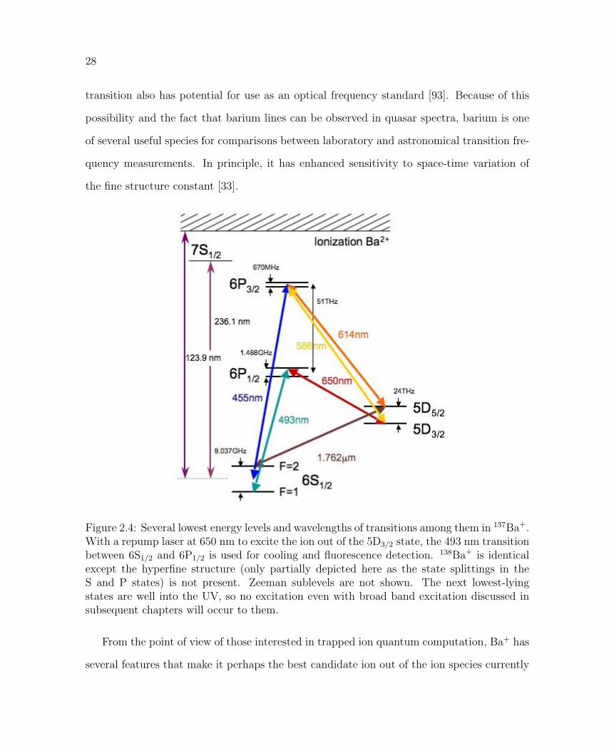
Figure 2.4: Several lowest energy levels and wavelengths of transitions among them in 137Ba+.With a repump laser at 650 nm to excite the ion out of the 5D3/2 state, the 493 nm transitionbetween 6S1/2 and 6P1/2 is used for cooling and fluorescence detection. 138Ba+ is identicalexcept the hyperfine structure (only partially depicted here as the state splittings in theS and P states) is not present. Zeeman sublevels are not shown. The next lowest-lyingstates are well into the UV, so no excitation even with broad band excitation discussed insubsequent chapters will occur to them.
From the point of view of those interested in trapped ion quantum computation, Ba+ has
several features that make it perhaps the best candidate ion out of the ion species currently
29
under investigations (Table 1.1). First of all, both the useful isotopes 138Ba+ and 137Ba+
are abundant enough that isotopically enriched samples are unnecessary (see Table 2.1).
Useful qubit schemes, both optical and hyperfine exist [26]. Secondly, the cooling structure
is extremely simple, requiring only two lasers both of which are in the visible and available
as standard diodes with one doubling stage. Most other ions have cooling transitions that
range from either very blue or well into the ultraviolet (UV). Besides simply being easier to
work with visible light, UV light does not transmit well in single-mode optical fiber, making
long-distance remote entanglement experiments [99] mediated by UV photons impossible.
Additionally, the low-lying D states are available for state detection by means of electron
shelving. These states decay only by electric quadrupole transitions and even then only at
very long wavelength (1.762 µm in the case of the 5D5/2 state), so the suppression of the
decay rate by a factor of λ5 makes them very long-lived.
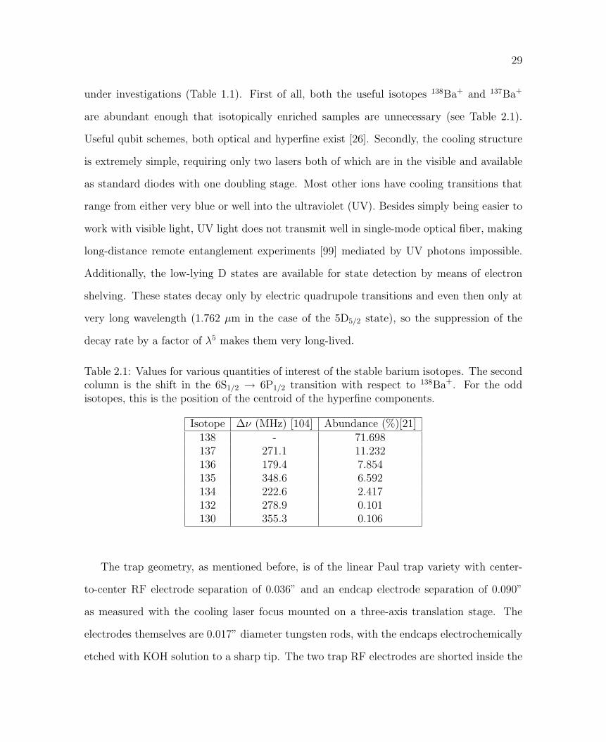
Table 2.1: Values for various quantities of interest of the stable barium isotopes. The secondcolumn is the shift in the 6S1/2 → 6P1/2 transition with respect to 138Ba+. For the oddisotopes, this is the position of the centroid of the hyperfine components.
Isotope ∆ν (MHz) [104] Abundance (%)[21]138 - 71.698137 271.1 11.232136 179.4 7.854135 348.6 6.592134 222.6 2.417132 278.9 0.101130 355.3 0.106
The trap geometry, as mentioned before, is of the linear Paul trap variety with center-
to-center RF electrode separation of 0.036” and an endcap electrode separation of 0.090”
as measured with the cooling laser focus mounted on a three-axis translation stage. The
electrodes themselves are 0.017” diameter tungsten rods, with the endcaps electrochemically
etched with KOH solution to a sharp tip. The two trap RF electrodes are shorted inside the
30
trap, as are the ground electrodes. While this diminishes the possible phase difference of
the RF between the two rods, it means that DC bias voltages applied to the RF and ground
electrodes that would be useful for micromotion compensation only shift the ion position
with their gradient. This form of excess micromotion compensation was attempted but
controlling micromotion remains a significant issue for this particular trap. The electrodes
are insulated from the trap structure with alumina spacers and the entire piece is placed
in a Kimball PhysicsTM 4-1/2” spherical octagon vacuum chamber with eight anti-reflection
coated fused silica viewports, two placed as close to the trap as possible to accommodate
photon collection optics, and the other six for laser access. Two additional ports are occupied
by RF and high voltage feed-through’s. The trap vacuum structure is baked for about a week
and continuously pumped by a Varian Star-CellTM 20 l/s ion pump and periodically by a
titanium sublimation pump. It has maintained UHV at a level of under 2 × 10⁻¹¹ torr
for several years with minimal effort, partially thanks to the fact that barium is itself an
excellent getter.
The RF for the trap is generated by a Hewlett Packard 8640B function generator amplified
to approximately 1-2 W and inductively coupled into the trap by means of a helical resonator
with a resonant frequency ΩRF = 2π × (12.38) MHz and a Q of several hundred [65]. The
ground electrodes can be accessed to allow modulation by means of an SMA coaxial connector
on the resonator. The high voltage feed-through for the endcaps and barium ovens is heavily
filtered by a network of low-pass pi-filters to prevent RF pickup from entering these power
supplies. Typical endcap voltage is 400-500 V for trapping and 700 V for cooling. After
considerable effort, we have found that trapping is facilitated by lower trapping potentials
while cooling improves at a slightly higher value. In addition to the RF and DC fields needed
for trapping, we apply a magnetic field of a few Gauss by running several amps of current
(typically 2.1 A) through a coil with a diameter of approximately 4” and about 200 turns
to break the Zeeman state degeneracy which would otherwise lead to dark states during

31
Doppler cooling [11]. Smaller coils on the two other spatial axes carry lower current to allow
steering of the magnetic field axis for optical pumping, more details on that to follow in
Chap. 6.
The barium atomic beam source is simply a 1 mm diameter, 1 cm long alumina tube
wrapped with a tungsten wire through which current is run to heat the natural barium in
the tube. To prevent coating optical access ports with barium which would render them
rather useless neutral density filters, the atomic beam is first collimated simply by placing
an aperture immediately in front of the oven. This aperture is also useful for keeping the
transverse velocity of the beam low to aiding in photoionization as well as for shielding the
trap itself from the heat radiated during loading. The neutral barium can be ionized by a
number of means. Initially, electron bombardment was used by an electron gun made from a
heated filament and accelerating plate. This is a less than ideal method as it tends to charge
dielectric surfaces in the trap contributing to unwanted patch potentials, and is not isotope
selective. A second method employed was an attempt at photoionization using a xenon flash-
lamp focused in the trap center. This lamp has considerable spectral content at wavelengths
shorter than 237.1 nm, the ionization threshold for barium. It was unclear whether this lamp
directly photoionized the barium in the atomic beam or if it created photoelectrons from the
rods, as the short wavelength photons were energetic enough to overcome the work function
of the tungsten, and especially the barium coating the trap.
Inspired by the success of two-step photoionization [100], an external cavity diode laser
(ECDL) at 791 nm was constructed. This laser excites barium on a 6s6s1S0 → 6s6p3P1
intercombination transition. From there a pulsed nitrogen laser at 337 nm excites the electron
to continuum, ionizing the barium. The 791 nm laser was aimed as perpendicular to the
atomic Ba beam as possible to minimize the first-order Doppler shift due to the atoms’
motion. Although the intercombination line has a 50 kHz linewidth in principle, a 640 MHz
FWHM width was observed while loading [27]. This is sufficiently narrow to separate 137Ba

32
Figure 2.5: Partial energy level diagram of neutral barium to highlight the two photoion-ization schemes employed over the course of this work. The two-photon scheme has theadvantage of isotope selectivity but is more sensitive to Doppler shift of the atomic beam.
from 138Ba, but 136Ba is loaded occasionally. Since the loading rate is sensitively dependent
on both the oven current and pulse rate of the N2 laser, both of these are kept quite low to
maximize the probability of loading only one ion at a time. The two photoionization schemes
are shown in Fig. 2.5.
Once a neutral barium atom is ionized near the trap center, it experiences the trapping
field of the quadrupole potential and quickly becomes localized as the cooling lasers bombard
it with photons. The main transition of interest is the 6S1/2 ↔ 6P1/2 transition at 493.4
nm. This light is generated by a home-built 200 mW 986 nm ECDL, frequency-doubled
in a non-critically phase-matched (temperature-tuned) potassium niobate (KNbO3) Type-I
ooe nonlinear crystal in a bow-tie enhancement cavity. The crystal itself is actually cut for
second harmonic generation of a slightly shorter wavelength, and owing to the steep slope of
the phase-matching temperature vs. laser wavelength, rather than heating to slightly over
room temperature the crystal is held near 60C. The cavity is locked using Pound-Drever-
Hall stabilization [12], with an error signal created by directly modulating the current on the

33
laser diode at 16 MHz through an isolation transformer and bias-T. The cavity specifications
and modulation circuit are pictured in Fig. 2.6 (a) and (b), respectively. Cavity locking is
achieved with a ADuC7020 digital microcontroller servo laid out in Fig. 2.7 [25]. For the
most efficient cooling, the polarization of this laser is elliptical and directed onto the ion
perpendicular to the quantization axis defined by the magnetic field (refer to the dipole
radiation patterns is Fig. 1.4 (a)).
Referring to the energy level diagram of Ba+, one finds that the 6P1/2 state can decay
to the 5D3/2 state via a dipole-allowed transition. The branching ratio for this decay is
approximately 27% [53] and the lifetime of the D state is 79 s [106]. This requires a second
laser at 649.7 nm to repump the ion back in to the 6P1/2 state. The 650 nm laser has the
same circuit to allow current modulation for the addition of sidebands for cooling 137Ba+.
The complete, closed cooling cycle is then comprised of the two wavelengths, 493 and 650
nm. The two colors are combined on a dichroic mirror and fiber coupled to send to the trap.
Even though the fiber coupling diminishes the power available by a significant fraction, it
has a number of advatages. It ensures perfect collinearity of the two beams, allows changes
to be made before the trap to the optical layout without disturbing the beam alignment to
the ion and serves to clean the mode to reduce halo and background scatter off trap surfaces.
After the fiber, there is approximately 50 µW of red light and and 5 µW of green, entirely
sufficient for cooling. When the ion is in this cycle, it fluoresces photons at 493 nm at a rate
of a few times 107/s. We collect these photons for state detection, as well as to simply know
that an ion is in the trap.
Before moving on to state detection, a word on laser stabilization is necessary. The
natural linewidth of the 6P1/2 state is approximately 20 MHz and although the quantity
of 493 nm light power broadens this, the line width and long-term drift of a free-running
ECDL would make Doppler cooling impossible. Therefore some sort of laser stabilization is
necessary. While it is painfully simple with neutral atoms, e. g. Cs and Rb where a simple

34
Figure 2.6: (a) Layout of second harmonic generation cavity for 493 nm cooling light. Thecurved mirror separation is 27 mm, just under the maximum allowed for stability as cal-culated by the transfer matrix approach [57]. Mode-matching is about 60%, cavity finesseapproximately 50 and free spectral range is approximately 880 MHz. (b) Bias-T for modu-lation of the diode lasers current for PDH error signal. The isolation transformer separatesthe Bias-T’s ground from the laser’s ground and the 1N914 and 1N5711 Schottky diodesprovide over-voltage and reverse bias protection respectively.
vapor cell provides a means of locking to the same species, ions are slightly more difficult.
Discharge tubes and hollow cathode lamps can be used, as well as performing Doppler-free
spectroscopy on molecular species with transitions in a similar wavelength range. The latter
was used for some time; a lock to diatomic tellurium for the green and iodine for the red.
These systems require the majority of the laser’s power be diverted to the lock and are

35
Figure 2.7: Cavity servo for SHG of 493 nm cooling light. The ADuC7020 is mounted on anevaluation board for easy uploading of scripts. In this case, it acts as both a ramp generatorfor cavity scanning and a digital integrator with a reacquire feature should the cavity fallout of lock. Adapted from [27].
cumbersome, often requiring a significant shift of relative laser and lock frequencies with
acoustic optic modulators to reach both the lock and cooling frequencies. The situation
becomes even more inconvenient when one wants to switch from one isotope to another.
Eventually the solution which proved most convenient was a digital system based on a High-
FinesseTM WS7 wavelength meter. The wavelength reading is digitized and sent to the
data acquisition system, the error signal calculated and the feedback returned to the laser’s
grating arm piezo via a 12-bit DAC. A fivefold voltage divider ensures that the step size
generated by the DAC is less than 1 MHz of laser frequency, which is actually well beyond
the resolution of the wavelength meter. The wavelength meter itself however was found
to drift in frequency, as shown in Fig. 2.8 where its measured frequency is referenced to a
stabilized helium-neon (HeNe) laser. Although temperature plays a role as well, atmospheric
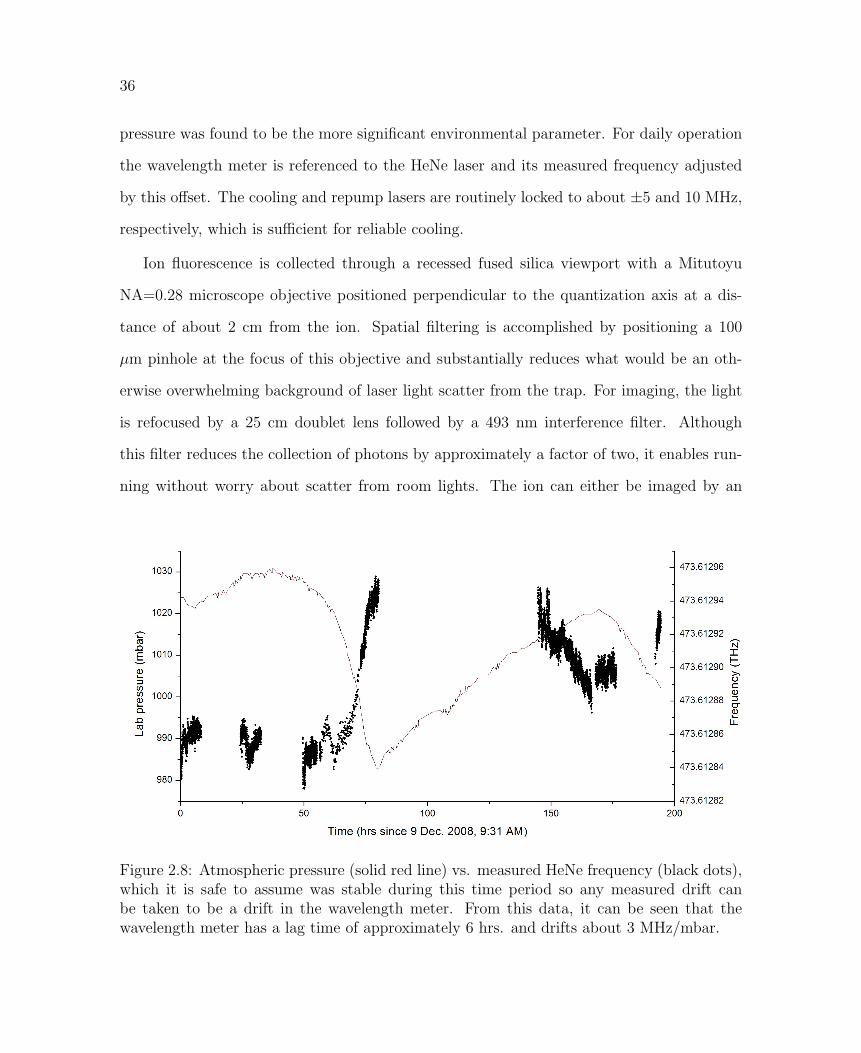
36
pressure was found to be the more significant environmental parameter. For daily operation
the wavelength meter is referenced to the HeNe laser and its measured frequency adjusted
by this offset. The cooling and repump lasers are routinely locked to about ±5 and 10 MHz,
respectively, which is sufficient for reliable cooling.
Ion fluorescence is collected through a recessed fused silica viewport with a Mitutoyu
NA=0.28 microscope objective positioned perpendicular to the quantization axis at a dis-
tance of about 2 cm from the ion. Spatial filtering is accomplished by positioning a 100
µm pinhole at the focus of this objective and substantially reduces what would be an oth-
erwise overwhelming background of laser light scatter from the trap. For imaging, the light
is refocused by a 25 cm doublet lens followed by a 493 nm interference filter. Although
this filter reduces the collection of photons by approximately a factor of two, it enables run-
ning without worry about scatter from room lights. The ion can either be imaged by an
Figure 2.8: Atmospheric pressure (solid red line) vs. measured HeNe frequency (black dots),which it is safe to assume was stable during this time period so any measured drift canbe taken to be a drift in the wavelength meter. From this data, it can be seen that thewavelength meter has a lag time of approximately 6 hrs. and drifts about 3 MHz/mbar.

37
Andor LucaTM electron-multiplied CCD camera, or the photons can be counted by a pair
of HamamatsuTM photomultiplier tubes (PMT’s), mounted on opposite output ports of a
polarizing beam splitter. The camera is mainly used for alignment and evaluation, while
the PMT’s are used for photon counting during experiments. A typical fluorescence signal,
demonstrating bright and dark counts and a histogram of the data is shown for illustrative
purposes in Figs. 2.9 (a) and (b).
Figure 2.9: (a) Time plot of single ion fluorescence while turning on and off the 650 nm laserto demonstrate the difference between bright and dark count rates. Shining the 1.762 µmlaser on the ion at the same time would produce a similar signal known as a “telegraph”only on a much faster time scale. (b) Histograms of multiple 20 ms exposures of the ion withdark counts near zero (non-zero due to background scatter) and bright counts averagingapproximately 75 counts. An appropriate cut-off for state discrimination here might bechosen at 40 counts.
The final laser in the system is a Koheras Adjustik TM thulium-doped fiber laser at 1.762
µm to address the 6S1/2 → 5D5/2 quadrupole transition. This laser is stabilized via a similar
PDH locking scheme as the cooling laser to a high-finesse ZerodurTM cavity enclosed in a
temperature controlled vacuum of about 10−6 Torr. The laser has a linewidth of < 5 kHz
and is therefore sufficiently narrow to address individual Zeeman or hyperfine transitions
between the ground and excited states. The 5D5/2 state has a lifetime of 32 s [106] during
which neither the 493 nm nor the 650 nm light is resonant with any available transition.
When the ion is in this state, it is said to be “dark,” since only background 493 nm light will

38
be collected by the PMT. If after the experimental cycle the ion is still in the cooling cycle
or “bright” state, it can be concluded that the 1.762 µm light was never resonant with any
available 6S1/2 → 5D5/2 sublevel transition. State selective detection via shelving can then
be performed by imposing a cutoff between “bright” and “dark counts.” Applying a second
pulse of 1.762 µm light will rotate the ion back down to the S state, bringing it back to the
cooling cycle for the experiment to continue.
The beam path of each laser between its output and the trap window contains a number
of optical elements to allow experimental control. For the 650 nm laser, 40 dB of optical
isolation and beam reshaping using an anamorphic prism pair is required. The light is then
focussed through an acoustic optic modulator. Besides introducing a frequency shift, the
AOM acts as a fast optical shutter (rise time <10 ns, as fast as 2 ns at the expense of diffrac-
tion efficiency), with the RF drive switched by Minicircuits ZYS-50D-R TTL-controlled
switches. The main portion of the 493 nm cooling light is sent through an AOM and then
coupled into a single mode fiber with the 650 nm light on a dichroic mirror. Before switching,
a small fraction of the 493 nm light is picked off to act as an optical pumping beam. This
light is switched independently of the main cooling beam. Before it enters the trap, there is
a Glan-Thompson polarizer and a quarter-wave plate to allow polarization control, which is
critical for optical pumping (more detail in Chap. 5). Details about the 1.762 µm laser are
in Section 5.3.
The entire experiment is computer-controlled through two National InstrumentsTM data
acquisition cards (a PCI-6220 and a PCIe-6351) which can alternately use hardware or on-
board timing and can be triggered with the phase of the wall voltage for magnetic-field
sensitive experiments. A multi-channel pulse sequencer based around a field programmable
gate array (FPGA) with accompanying direct digital synthesizer (DDS) has also been de-
veloped and allows for the creation of multiple signals of arbitrary amplitude, phase and
envelope with user-defined phase and timing relations to one another. A block diagram of

39
Figure 2.10: Block diagram layout of the entire experimental apparatus, without collectionand imaging optics for clarity. See text for a description of the cooling, detection andionization lasers. The function of the Ti:Sapphire laser will be addressed in Chap. 3.
the entire system is shown in Fig. 2.10.

40

3 ULTRAFAST INTERACTIONS
If you can’t get rid of the skeleton in your closet, you’d best teach it to dance.
- George Bernard Shaw
The previous chapter gave an outline of the elements of the experimental apparatus that
pertain to cooling, state manipulation and detection. The light sources that perform these
tasks are all continuous wave, or CW. Another class of lasers equally useful in quantum
computation with trapped ions is the family of mode-locked lasers, which emit intense,
coherent pulses of light as short as a few femtoseconds if extreme care is taken in their
design. Peak power in such lasers can be extremely high (up to megawatts and even higher
with regenerative amplification) owing to the brief duration of the pulse. The first mode-
locked lasers were Argon ion-pumped dye lasers in the 1970’s, followed by the creation
of the modern (though aging) work-horse of the field, the titanium (Ti3+)-doped sapphire
(Ti:Sapphire) laser, developed in 1986 [75]. Other solid-state mode-locked lasers exist, YAG
and vanadate lasers with various rare-earth dopants or the family of vibronic lasers such
as forsterite, alexandrite, LiCAF and LiSAF where the chromium ion plays the role of
titanium just to name a few. However, none have the broad gain bandwidth (150 THz)
of the Ti:Sapphire laser. More and more, mode-locked fiber lasers are replacing solid-state
systems because of their robust operation and low maintenance, although they have yet to
reach single optical cycle pulse lengths.
Mode-locked lasers have found their way into the field of trapped ion quantum compu-
41

42
tation in a number of ways because of the fact that the high electric field intensity can very
quickly drive excitations in ions. Recall that the Rabi frequency of a particular laser-driven
transition is proportional to the local electric field at the ion. Also, being able to drive an
ion into an excited state much fast than the characteristic decay time of that state (typically
< 10 ns for a radiative transition) has enabled many protocols that require single photon
emission. Remote entanglement [72], quantum teleportation [80], ultrafast quantum gates
[50] and single-pulse driven Raman transitions [16] are all applications of pulses much shorter
than the lifetime of radiative transition useful for quantum computation with trapped ions.
3.1 Mode-locked lasers
All mode-locked pulsed lasers operate on the same principle, but achieve their operation in
a variety of ways. This discussion will be as general as possible, but is geared toward the
operation of Ti:Sapphire lasers since the entirety of the work presented here was performed
with such a laser. The basic design of a mode-locked laser is the same as any CW laser,
that is a reflective optical cavity with one lossy side built around a gain medium pumped
optically with continuous, coherent light. The gain medium here in contrast to CW lasers,
is specifically chosen to have a broad gain bandwidth (up to 100 THz). For comparison,
an atomic transition line in a gas laser or the band gap between conduction bands in a
semiconductor have widths of 100’s of MHz. A Ti:Sapphire laser has the broadest gain
spectrum of any solid-state system and can in principle operate from 600 nm to nearly 1
µm, although the Ti3+ dopant fraction and other properties of the crystal generally limit
particular lasers to slightly narrower regions of this spectrum. The term “mode-locked”
refers to the longitudinal cavity modes, which form a comb of frequencies spaced by the free
spectral range (FSR) of the cavity with length L (FSR ≡ c2L), which are made to oscillate
with a fixed phase relationship to one another. The frequency domain picture of the laser’s

43
operation then is a comb of equally spaced modes with an overall intensity envelope given by
the gain profile of the lasing medium and laser cavity parameters. The time domain picture
is then is a train of equally spaced pulses with a pulse width τp = TBPN∆ν , where TBP refers
to the time-bandwidth product, a factor of order unity specific to the functional shape of
the pulse, N the number of simultaneously lasing modes in the cavity and ∆ν the spectral
bandwidth of the gain medium. Ti:Sapphire lasers (and most other passively mode-locked
lasers for that matter) typically have or are assumed to have a hyperbolic secant electric
field temporal profile with a TBP = 0.315 [20].
The mode-locking is achieved by a number of ways which fall into two broad categories,
active and passive mode-locking. Actively mode-locked lasers make use of some sort of
externally-timed optical shutter, such as an AOM, synchronized to the round-trip time of
a pulse in the cavity. Passively mode-locked lasers use a material, a saturable absorber,
which is only transparent to light of sufficiently high intensity, and therefore make the cavity
unfavorable for CW operation. Such materials have a significantly high third-order com-
ponent to their electric susceptibility tensor χ(3) that they acquire an intensity dependence
to their index of refraction ∆n = λKI, where λ and I are the wavelength and intensity of
the light, respectively, and K is known as the Kerr constant of the medium. The trick is
then to make the cavity itself unstable for CW operation, often done by closing a slit on the
circulating beam or adjusting the length of the cavity around the Ti:Sapphire crystal. Lasers
mode-locked in this way are referred to as Kerr-lens mode-locked lasers and tend to have
the shortest pulse lengths attainable. The last element necessary for stable mode-locked
operation is a means by which to compensate the group velocity dispersion (GVD) that
occurs within the laser cavity due to the fact that the many different wavelengths operating
concurrently experience wavelength-dependent indices of refraction which would otherwise
lead to relative and randomly-evolving phases of the different frequency components. This is
exacerbated by the self phase modulation (SPM) introduced by the Kerr effect itself which

44
Figure 3.1: Mode-locked Ti:Sapphire laser used for this experiment based on CoherentMiraTM. Bi Fi birefringent filter for frequency tuning, ML slit used for chopping out CWmode and starting mode-locked operation, GVD comp prism pair for dispersion compensa-tion, Sync PD fast photodiode used to synchronize pulse picking AOM to laser for experi-ments
it has already been noted is an intensity dependent index of refraction. GVD and SPM are
compensated by either prism pairs or “chirped” mirrors which allow the slower wavelengths
(blues) to “catch up” to the faster ones (reds).
The laser used for the majority of the work presented here is a design based on a heavily
modified Coherent MiraTM. During the course of this work it has been pumped either by a
single 15 W Spectra-Physics MilleniaTM at 532 nm or two 5 W versions of the same laser
focussed into opposite ends of the Ti:Sapphire crystal. It has a repetition rate of 76 MHz and
a pulse width of 400 fs. This corresponds to a spectral width of about 125 GHz assuming
transform-limited pulses. By design, this is broad enough to cover the frequency splitting
between hyperfine levels of the ground state of 137Ba+ (8.037 GHz) but not so wide that
transitions to undesired excited states are driven (6P states have a fine structure splitting
of over 50 THz). By changing mirror sets, the laser can be made to operate and mode-lock
at any wavelength between 860 and 1020 nm, although the only two useful wavelengths are
910 and 986 nm, twice the wavelength of the 6S1/2 → 6P3/2 and→ 6P1/2 transitions in Ba+,
respectively. The pulses are frequency-doubled via single pass through a β-BaB2O4 crystal.
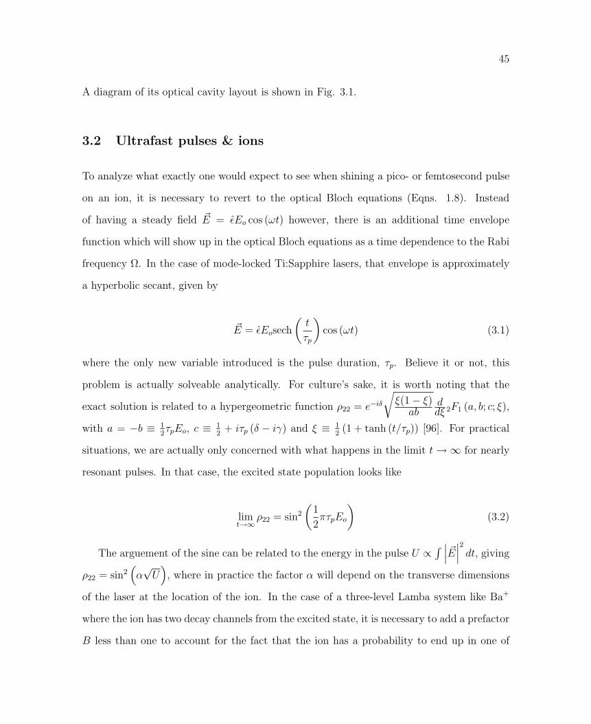
45
A diagram of its optical cavity layout is shown in Fig. 3.1.
3.2 Ultrafast pulses & ions
To analyze what exactly one would expect to see when shining a pico- or femtosecond pulse
on an ion, it is necessary to revert to the optical Bloch equations (Eqns. 1.8). Instead
of having a steady field ~E = εEo cos (ωt) however, there is an additional time envelope
function which will show up in the optical Bloch equations as a time dependence to the Rabi
frequency Ω. In the case of mode-locked Ti:Sapphire lasers, that envelope is approximately
a hyperbolic secant, given by
~E = εEosech
(t
τp
)cos (ωt) (3.1)
where the only new variable introduced is the pulse duration, τp. Believe it or not, this
problem is actually solveable analytically. For culture’s sake, it is worth noting that the
exact solution is related to a hypergeometric function ρ22 = e−iδ√ξ(1− ξ)ab
ddξ 2F1 (a, b; c; ξ),
with a = −b ≡ 12τpEo, c ≡ 1
2+ iτp (δ − iγ) and ξ ≡ 1
2(1 + tanh (t/τp)) [96]. For practical
situations, we are actually only concerned with what happens in the limit t→∞ for nearly
resonant pulses. In that case, the excited state population looks like
limt→∞
ρ22 = sin2
(1
2πτpEo
)(3.2)
The arguement of the sine can be related to the energy in the pulse U ∝∫ ∣∣∣ ~E∣∣∣2 dt, giving
ρ22 = sin2(α√U)
, where in practice the factor α will depend on the transverse dimensions
of the laser at the location of the ion. In the case of a three-level Lamba system like Ba+
where the ion has two decay channels from the excited state, it is necessary to add a prefactor
B less than one to account for the fact that the ion has a probability to end up in one of
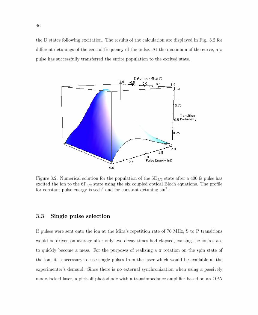
46
the D states following excitation. The results of the calculation are displayed in Fig. 3.2 for
different detunings of the central frequency of the pulse. At the maximum of the curve, a π
pulse has successfully transferred the entire population to the excited state.
Figure 3.2: Numerical solution for the population of the 5D5/2 state after a 400 fs pulse hasexcited the ion to the 6P3/2 state using the six coupled optical Bloch equations. The profilefor constant pulse energy is sech2 and for constant detuning sin2.
3.3 Single pulse selection
If pulses were sent onto the ion at the Mira’s repetition rate of 76 MHz, S to P transitions
would be driven on average after only two decay times had elapsed, causing the ion’s state
to quickly become a mess. For the purposes of realizing a π rotation on the spin state of
the ion, it is necessary to use single pulses from the laser which would be available at the
experimenter’s demand. Since there is no external synchronization when using a passively
mode-locked laser, a pick-off photodiode with a transimpedance amplifier based on an OPA

47
380 for approximately 90 MHz bandwidth was installed behind an imperfect laser cavity
(see Fig. 3.1) mirror to pick up the pulse signal and synchronize the laser’s operation to
the experiment. The resulting signal is too small to be recognized for control by the DAQ
system so must be amplified to a level which is TTL-compatible. This is accomplished with
a chain of high-speed devices consisting of a UA733 video amplifier, a MAX933 high-speed
comparator and finally a DS1040-A15 single-shot pulse generator with 5 ns pulse width.
Even with fast electronics, the dead time of the DS1040-A15 causes it to miss every second
pulse, effectively making the fastest possible operation equal to half the repetition rate of
the Mira. When needed for the experiment, single-shot pulses from the DAQ card enter one
input terminal of a Potato semiconductors PO74G08A 1.125 GHz bandwidth AND gate and
the synchronization pulse train from the laser enter the other. The resulting pulse with 5 ns
duration triggers an HP8310B pulse generator with variable delay. This allows monitoring of
selected pulses on a fast photodiode to ensure that the trigger pulse is centered on the laser’s
pulse train. The same RF signal generators, amplifiers, switches and AOM’s as are used to
Figure 3.3: Pulse picker electronics, the function of individual elements is described in thetext. The counter is used to monitor the trigger out from the HP 8310B and provides a wayto count the number of times the switch is triggered. Approximately 3% of the trigger pulsesare missed and these counts were removed from experiments.

48
switch on and off the cooling lasers are used to provide an optical shutter triggered by the
TTL pulses from the 8310. Rather than being optimized for maximum deflection efficiency,
the AOM in the beam path of the Mira is optimized for the fastest possible rise time, although
it is still the bottleneck in the overall speed of the system and incomplete switching on and
off leads to the leakage of laser pulses (not more than ∼ 3% of the maximum intensity of
the main peak) on either side of the selected pulse. These are highly attenuated in the SHG
process which scales with the square of the intensity. The RF drive power, and hence the
energy per laser pulse, can be adjusted via a DAC-controlled Minicircuits ZX73-2500 voltage
variable attenuator (VVA). Fig. 3.3 shows the chain of electronics pictorially. A protocol
to use pulse sequencer’s capability to execute a phase-locked loop is under development and
would in principle replace the DAQ trigger pulse and AND gate, greatly simplifying the
operation of the system.
3.4 Rabi flop at 455 nm
The first experiments performed using the mode-locked pulses from the Mira were to excite
the ion from the 6S1/2 state to the 6P3/2 at 455.4 nm by frequency doubling 910.8 nm
Ti:Sapphire laser pulses rather than 6P1/2, because the available pump power was insufficient
to provide enough power to mode-lock the laser at 986 nm. The experiment was performed
by first turning off the cooling lasers, the 650 nm repump laser a few microseconds after
the 493 nm cooling laser to ensure pumping to the ground state rather than the D state. A
single pulse at 455.4 nm was then sent onto the ion, exciting it to the 6P3/2. From there,
three allowed decay channels exist, the first back to the 6S1/2 state at 455.4 nm, the second
to the 5D5/2 at 614.2 nm and the third to the 6D3/2 at 585.5 nm. If the ion decayed to either
the ground state or to 5D3/2, it would appear bright when the cooling lasers were switched
back on immediately after the pulse. If however, it went to the 5D5/2 state, it would be out

49
of the cooling cycle and appear dark. A high-power Luxeon Star orange LED with a central
wavelength near 614 nm provided a means to excite the ion out of the dark state to begin
a new run of the experiment. The process was repeated for different attenuation values on
the VVA from the maximum 455nm pulse energy at about 1.6 nJ per pulse down to where
no shelving was observed at about 0.05 nJ per pulse.
Figure 3.4: Data obtained from single 455 nm laser pulse excitation of the 6S1/2 → 6P3/2
transition. The vertical axis is the fraction of times the ion was not fluorescing followingthe incident pulse, meaning that it was in the 5D5/2 state. Vertical error bars are statistical,given by the binomial variation in dark probability. Horizontal error bars are due to thevariation in pulse energy which arise both from a slight non-constant intensity envelope ofthe pulses from the laser and from the finite rise time of the pulse picking AOM. The solid
line is a two parameter fit to the function Pdark = B sin2(α√U/2
).

50
The resulting data were binned an fit to the function Pdark = B sin2(α√U/2
), where
B is the branching ratio for the fraction of the time that the ion decays to the dark 5D5/2
rather than back into the cooling cycle and α simply corresponds to the shelving efficiency.
So besides simply being a demonstration of the ability to excite the ion from the ground
state to the excited P state with unit probability at a particular pulse energy given by
the location of the maximum in Fig 3.4, this experiment when combined with a second
experiment described in the following section provides a means to measure the branching
ratios from 6P3/2 state and hence, the transition amplitudes and radial matrix elements.
The branching fraction for the 6P3/2 → 5D5/2 decay was found to be 0.215 ± 0.0047 and α
equal to 3.41±0.07 nJ−1/2. The value of B moreover was robust against fluctuations in α up
to the observed 10%. It also proved not to change due to the small pulses on either side of
the main selected pulse. This concern was laid to rest through numerical integration of the
Bloch equations (see section and Fig. 3.2); the side pulses simply contribute to a non-zero
dark probability at a pulse energy corresponding to a 2π rotation but do not have any effect
on the maximum value of the curve which is simply given by the branching ratio.
3.5 Branching ratios from 6P3/2
A second experiment was needed to determine the absolute values of all three branching
ratios, since the Rabi flop determined the fraction that decayed to the 5D5/2 state, leaving
the two decay channel to 6S1/2 and 5D3/2 indistinguishable. This was done by weakly exciting
the ion to the 6P3/2 state using trains of highly attenuated pulses at 455 nm of various lengths
from 0.1 to 10 ms and 1.6 to 3.4 mW of average power. This relaxed the requirement that
single pulses be selected from the Mira. This left decays to the D state indistinguishable,
since only in the asymptotic limit could it be that ion was excited to the 6P3/2 state with
high probability. The functional form of the dark probability expected vs. exposure time

51
can be calculated from the probability of excitation for a single pulse, given by the already
frequently used equation Pexc = sin2(α√U/2
)which can be expanded for low energy and
hence small arguement of the sine to be Pexc ≈ α√U . If the excited state has a probability
B for decay to a dark state and 1− B to a bright state, the rate of pumping into the dark
state is given by Bα√EfREP , where fREP is the repetition rate of the laser. A steady-state
dark population Pdark = Bα√E
∞∑n=0
e−nγ/fREP = Bα√E
e−γ/fREP
1− e−γ/fREPwill accumulate due to
the sum of decaying exponentials with a characteristic lifetime γ for decay form the excited
Figure 3.5: Characteristic data for the weak excitation experiment performed to determinea value for the branching ratio of D state decays. The experiment was repeated to establisha statistically robust value for the asymptotic dark state probability. The fit is to theexpected form of the function discussed in the text Pdark = ∆ + B
(1 + e−λt
). Error bars
include both the statistical uncertainty from binomial probability and a 0.5% systematicuncertainty arising mainly from de-excitation due to cooling light leakage and backgroundgas collisions.

52
state in between pulses. The sum can be taken to infinity because the time between pulses
and the lifetime for the atomic decay are both much shorter than the total exposure time.
The rate of accumulation into the dark state population is then γPdark. The total rate of
pumping to the dark state, or shelving, is then the sum of Pexc and Pdark which can be
integrated to give the population ρdark, and hence the probability of finding the ion dark
after the train of pulses has passed. The functional form expected for the probability that
the ion is dark, after all is said and done, is Pdark = ∆ +B(1 + e−λt
), where ∆ is any offset
from zero probability at zero pulse duration due to false dark counts and λ is a parameter
which depends on the pulse intensity, repetition rate and decay rate from the excited state.
A representative data set for different exposure times is shown in Fig. 3.5.
The results of the weak excitation experiment are a ratio for each of the D state decays
to each other, excluding decays to the S state, determined from the asymptotic dark state
probability related to the B coefficient. The relative strengths are 0.881 and 0.119 for
5D5/2 and 5D3/2, respectively. Combining these ratios with the absolute value for the 5D5/2
decay from the Rabi rotation experiment and the fact the total ratio must equal unity, the
absolute values for the branching ratios to 6S1/2, 5D3/2 and 5D5/2 are 79.6, 2.9 and 21.5%
respectively. From the three branching ratios, summarized again with uncertainties in Table
3.1, transition rates and the dipole matrix elements can be calculated for the three transitions.
The branching ratios are simply algebraic ratios of the three absolute transition amplitudes
for the decays, with the constraint that the lifetime of the excited state τi is given by the
inverse of the sums of all amplitudes for decays from that state, τi =(∑
f Afi
)−1
. From
knowledge of the lifetime of the 6P3/2 state, given in [84] to be 6.32(10) ns, the transition
amplitudes for the 6P3/2 → 6S1/2, → 5D3/2 and → 5D5/2 are calculated and given in the
final column of Table 3.1. From the transition strengths, the radial dipole matrix elements
(Sect. 1.3) can be calculated

53
⟨6P3/2
∣∣∣∣∣∣DE1
∣∣∣∣∣∣ f⟩ =
√giλ3Afi
2.0261× 10¹⁸(3.3)
where gi is the degeneracy of the excited state (4 in the case of 6P3/2), λ is the transition
wavelength and the numerical factor a conversion to atomic units where eao = 1 [49, 48]. The
three matrix elements are then⟨6P3/2
∣∣∣∣ DE1
∣∣∣∣6S1/2
⟩= 4.720±0.040,
⟨6P3/2
∣∣∣∣ DE1
∣∣∣∣5D3/2
⟩=
1.349± 0.036 and⟨6P3/2
∣∣∣∣ DE1
∣∣∣∣5D5/2
⟩= 3.945± 0.066.
Table 3.1: Measured values for branching ratios from 6P3/2
Transition Relative Radial matrix element Rate6P3/2 → strength (a.u.) Afi × 109s−1
6S1/2 0.756± 0.046 4.720± 0.040 0.1196± 0.00205D3/2 0.029± 0.0015 1.349± 0.036 0.004589± 0.000255D5/2 0.215± 0.0064 3.945± 0.066 0.03402± 0.00115
The main use for improved values of these matrix elements is in experimental confirmation
of the values calculated and used in the calculation of the parity-nonconserving amplitude
A (E1)PNC in the 6S1/2 → 5D3/2 transition. The amplitude itself is given in second-order
perturbation theory as a sum over intermediate state matrix elements of both the dipole
(DE1) and parity-nonconserving weak charge (HPNC) Hamiltonians.
A (E1)PNC =∑
n6=6S1/2
⟨5D3/2
∣∣ DE1 |n〉 〈n| HPNC
∣∣6S1/2
⟩E6S1/2
− En(3.4)
+∑
n6=5D3/2
⟨6S1/2
∣∣ DE1 |n〉 〈n| HPNC
∣∣5D3/2
⟩E5D3/2
− En
[91]
The largest contributions come from terms involving the 6P1/2 and 6P3/2 states and make up
90 and 8 % of the overall amplitude. Two of the radial matrix elements,⟨6P3/2
∣∣∣∣ DE1
∣∣∣∣5D3/2
⟩
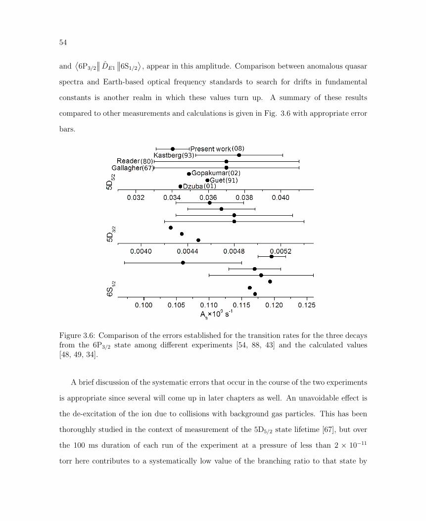
54
and⟨6P3/2
∣∣∣∣ DE1
∣∣∣∣6S1/2
⟩, appear in this amplitude. Comparison between anomalous quasar
spectra and Earth-based optical frequency standards to search for drifts in fundamental
constants is another realm in which these values turn up. A summary of these results
compared to other measurements and calculations is given in Fig. 3.6 with appropriate error
bars.
Figure 3.6: Comparison of the errors established for the transition rates for the three decaysfrom the 6P3/2 state among different experiments [54, 88, 43] and the calculated values[48, 49, 34].
A brief discussion of the systematic errors that occur in the course of the two experiments
is appropriate since several will come up in later chapters as well. An unavoidable effect is
the de-excitation of the ion due to collisions with background gas particles. This has been
thoroughly studied in the context of measurement of the 5D5/2 state lifetime [67], but over
the 100 ms duration of each run of the experiment at a pressure of less than 2 × 10⁻¹¹
torr here contributes to a systematically low value of the branching ratio to that state by
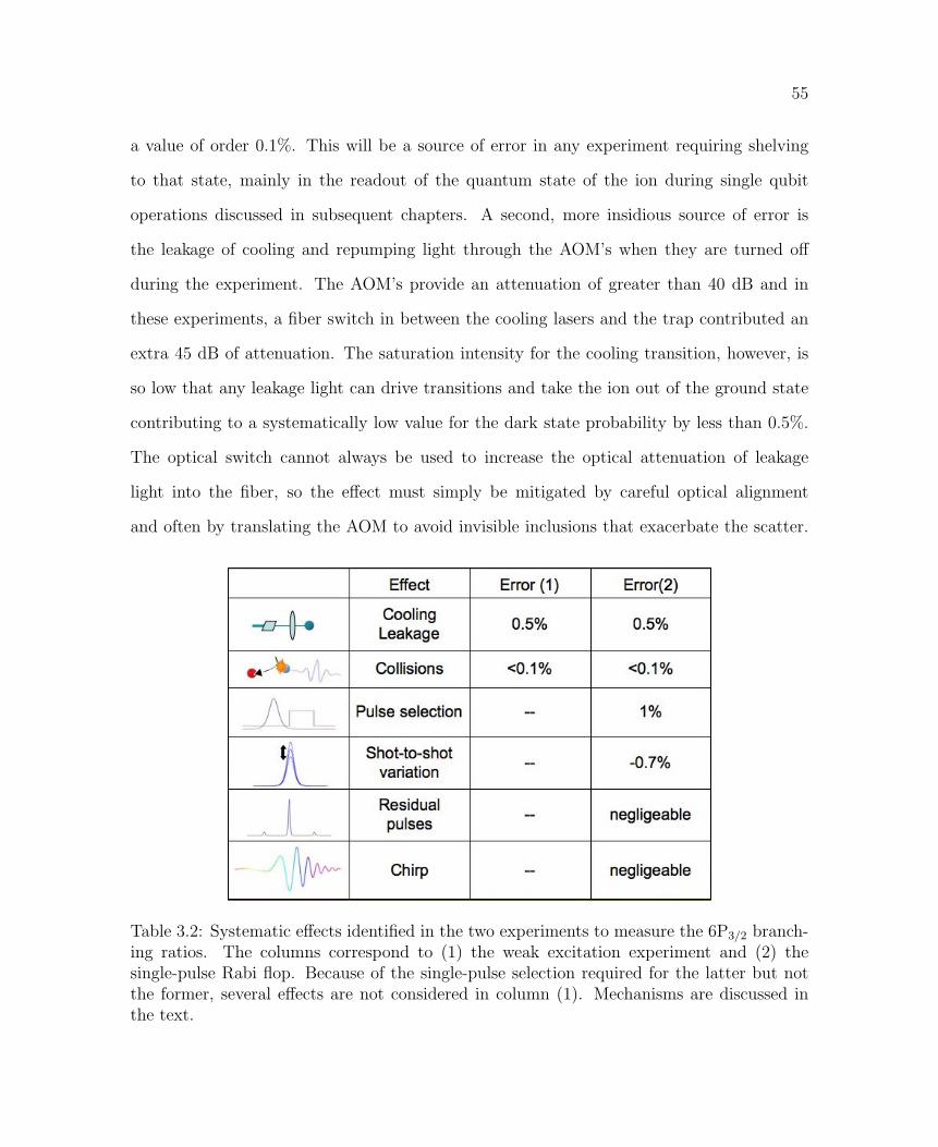
55
a value of order 0.1%. This will be a source of error in any experiment requiring shelving
to that state, mainly in the readout of the quantum state of the ion during single qubit
operations discussed in subsequent chapters. A second, more insidious source of error is
the leakage of cooling and repumping light through the AOM’s when they are turned off
during the experiment. The AOM’s provide an attenuation of greater than 40 dB and in
these experiments, a fiber switch in between the cooling lasers and the trap contributed an
extra 45 dB of attenuation. The saturation intensity for the cooling transition, however, is
so low that any leakage light can drive transitions and take the ion out of the ground state
contributing to a systematically low value for the dark state probability by less than 0.5%.
The optical switch cannot always be used to increase the optical attenuation of leakage
light into the fiber, so the effect must simply be mitigated by careful optical alignment
and often by translating the AOM to avoid invisible inclusions that exacerbate the scatter.
Table 3.2: Systematic effects identified in the two experiments to measure the 6P3/2 branch-ing ratios. The columns correspond to (1) the weak excitation experiment and (2) thesingle-pulse Rabi flop. Because of the single-pulse selection required for the latter but notthe former, several effects are not considered in column (1). Mechanisms are discussed inthe text.

56
Asynchronicity between the pulse picker gate and the actual optical pulse from the laser,
likely resulting from too short of an overlap between the computer trigger pulse and the
pulse train coming from the DS1040-A15 to trigger the AND gate, resulted in about a 1%
systematic error in the branching ratio involved in the Rabi rotation experiment. Shot-to-
shot variation in pulse energy, found to be of order 10% contributed to a systematically
low value for the branching ratio by a factor of about -0.7%. This variation is larger than
measured for the pulse train of the laser itself and likely arises from the finite rise time
of the pulse picker AOM. Better synchronization through the use of the phase-locked loop
capability of the pulse programmer will likely eliminate the first problem and alleviate the
second when this method of excitation is used to drive pulsed Rabi oscillation for coherent
coupling of photon modes with the ion’s spin, following the methods used for 111Cd+ [68]
and 171Yb+ [72]. Residual pulses on either side of the selected pulse which are of order 3%
the peak intensity of the main peak were found through the simulation in Sec. 3.2 to have
no effect on the maximum attainable shelving efficiency but only to add some residual dark
state population at an energy corresponding to a 2π pulse which would otherwise have zero
probability there. Additional effects related to the pulses, such a frequency chirp, do not
have any effect.
3.6 Ultrafast excitation at 493 nm
Since the goal of exciting the ion with ultrafast pulses is not simply to measure quantities
in Ba+, but rather to generate entangled ion-photon and ultimately ion-ion pairs, drive
stimulated Raman transitions with the different frequency components in the pulse or to
realize ultrafast quantum gates [44, 29], it is necessary to pursue a means by which to generate
mode-locked pulses at 986 nm to frequency double to resonance with the 6S1/2 → 6P1/2
rather than 6P3/2 transition. This was accomplished by adding a second pump laser counter-

57
Figure 3.7: Ion fluorescence as a function of RF attenuation for illumination with 493 nmmode-locked pulses at a repetition rate of 8 MHz. Vertical error bars are the Poissonianvariance in the counts for 20 trials per attenuation value. Dark counts were also recorded byturning off the red laser while the pulses were still incident on the trap and subtracted fromthe background. Horizontal error bars reflect the ±5% variation in pulse energy observed inthe excitation at 455 nm, although this only reflects an upper bound.
propagating with the first and replacing the output coupler of the Ti:Sapphire laser with
one more restrictive at the longer wavelength. The pulses were then sent onto the ion at
a repetition rate decreased by a factor of ten with the 493 nm cooling laser turned off but
the 650 nm repump laser left on. This is identical to the normal closed cooling cycle, albeit
with the 650 nm laser providing the Doppler cooling and the pulsed laser at 493 nm serving
as a repump, and ion fluorescence at 493 nm could be observed on the PMT. A plot of ion
fluorescence as a function of attenuation on the VVA is given in Fig. 3.7. As attenuation
decreases, more fluorescence is observed.
Generating ion-photon entangled pairs entails careful selection of states, polarization of
excitation pulses and the direction from which they should be focussed onto the ion and the
resulting photons be collected. Dipole radiation patterns plotted in Fig. 1.4(a) determine the
probability of excitation given the angle of incidence. It would, for example, be impossible to
drive π transitions along the magnetic field axis or to observe those decays. Selection rules
can be used to the advantage of the experimenter as in the first ion-photon entanglement

58
scheme pictured in Fig. 3.8 where there is no mixing of ∆mF = 0 decays. This creates
a unique entangled state ψion−photon = 1√2
(|F = 2,mF = 0; νred〉+ |F = 1,mF = 0; νblue〉)
if all circularly polarized photons are filtered out. This is known as a photonic frequency
qubit. A second scheme to illustrate the difficulty of generating entanglement in this way
using the 6P3/2 state is shown in Fig. 3.7 on the right. Here a circularly polarized pulse
excites the ion to the MJ = +3/2 state in the upper manifold which can no longer decay
to the ground state except by emitting a circularly polarized photon. Since there is only
one possible decay, there is no possible entanglement. Here instead an entangled ion-photon
state exists on the 614 nm decay. If linearly polarized photons are filtered out, the state can
be calculated using the formulae for transition strengths from Sec. 1.3, and is found to be
ψion−photon =
(10√101
∣∣∣mJ = 52;σ−
⟩+ 1√
101
∣∣∣mJ = 12;σ+
⟩). This is known as a photonic
polarization qubit, albeit a poor one due to the fact that one decay is ten times more
likely than the other. This situation is also less than ideal because decays to this state are
significantly less likely than those to the ground state, cutting down on the probability of
generating the state in the first place, and the entangled state will decay in the characteristic
lifetime of the 5D5/2 state. The desirable qualities of an ion-photon entanglement scheme
are then
1) maximal entanglement (i. e. generation of one of the Bell states)
2) no extra decays that must be ignored
3) ion qubit states in the ground state
4) unwanted excitations excluded by selection rules
Despite the fact that hyperfine and optical qubits have been demonstrated in 137Ba+, a
third qubit that perfectly fulfills these criteria for the generation of entangled ion-photon
pairs with ultrafast excitation is a qubit encoded in the Zeeman sublevels of the spinless
138Ba+ isotope, as will be described in the final chapter.

59
Figure 3.8: Two entanglement schemes, left a frequency qubit in 137Ba+, right a polarizationqubit in 138Ba+. Individual Zeeman levels can no longer be ignored, as they were in theenergy level diagram Fig. 2.4, since transitions strengths and selection rules given in Fig.1.5 determine the entangled states that can be created.

60

4 SINGLE PHOTON SOURCE
It is kind of fun to do the impossible.
- Walt Disney
Besides the requirements for the generation of ion-photon entangled pairs mentioned in
the final section of the previous chapter, i. e. uniqueness of excitation and decay channels,
maximal entanglement and a long-lived ionic qubit, another critical point in the problem is
that each excitation produce no more than one photon. As previously mentioned, the goal
of using mode-locked pulses to push excitation probability to unity is ultimately to use those
photons as a means by which to carry information about the ion’s spin state. In ion-photon
entanglement schemes, if the ion produces two photons, the combined state will be mixed
and useless. Likewise in ion-ion entanglement, where the photons are made to interfere on
a non-polarizing beam splitter to remove which-way information to project the ions into a
combined entangled state, if more than one photon per ion is emitted, the state will be mixed.
Additionally, the photon collection and detection apparatus must be sufficiently sensitive to
single photons if the protocol is to generate entangled pairs at a reasonable rate.
Both to verify the creation of single photons and ultimately to entangle the spin states of
two ions, the optical setup for photon detection requires a slight change of elements before
the PMT pair. In this case, we use a non-polarizing beam splitter so that the two photonic
channels are identical. Only in the case that we want to perform a measurement of the
photon polarization state, for instance to verify that emitted photons are in fact entangled
61
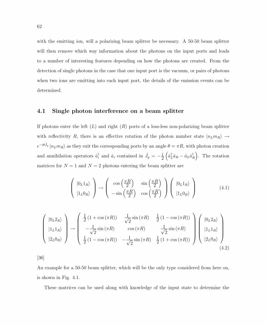
62
with the emitting ion, will a polarizing beam splitter be necessary. A 50-50 beam splitter
will then remove which way information about the photons on the input ports and leads
to a number of interesting features depending on how the photons are created. From the
detection of single photons in the case that one input port is the vacuum, or pairs of photons
when two ions are emitting into each input port, the details of the emission events can be
determined.
4.1 Single photon interference on a beam splitter
If photons enter the left (L) and right (R) ports of a loss-less non-polarizing beam splitter
with reflectivity R, there is an effective rotation of the photon number state |nLmR〉 →
e−iθJy |nLmR〉 as they exit the corresponding ports by an angle θ = πR, with photon creation
and annihilation operators a†i and ai contained in Jy = − i2(a†LaR − aLa
†R
). The rotation
matrices for N = 1 and N = 2 photons entering the beam splitter are
|0L1R〉
|1L0R〉
→ cos
(πR2
)sin(πR2
)− sin
(πR2
)cos(πR2
) |0L1R〉
|1L0R〉
(4.1)
|0L2R〉
|1L1R〉
|2L0R〉
→
12 (1 + cos (πR)) 1√
2sin (πR) 1
2 (1− cos (πR))
− 1√2
sin (πR) cos (πR) 1√2
sin (πR)
12 (1− cos (πR)) − 1√
2sin (πR) 1
2 (1 + cos (πR))
|0L2R〉
|1L1R〉
|2L0R〉
(4.2)
[36]
An example for a 50-50 beam splitter, which will be the only type considered from here on,
is shown in Fig. 4.1.
These matrices can be used along with knowledge of the input state to determine the

63
Figure 4.1: The four output states from a 50-50 non-polarizing beamsplitter obtained usingEq. 4.2 with the input state |1L1R〉.
form of the photon distributions measured on the output ports of the beamsplitter. If the
photons are created in a spatial-temporal mode ξ (~r, t) at input port i (an index indicating
either L or R) by decays from an excited state with lifetime τ by a series of N laser pulses
with a repetition time trep between them, the electric field operator is given by
E+i (t) =
N∑n=1
A√τξ (~r, t) e−
12
(t−ntrep)/τΘ (t− ntrep) a(n)i (4.3)
The factors A and 1/√τ serve to account for the amplitude to detect photons and to nor-
malize the photon detection probability to a unitless quantity. Θ (t− ntrep) is a Heaviside
unit step function representing the probability of photon creation at each repetition of the
experiment. The number state of photons at port i is a product of the N repetitions of the
experiment along with the implicit assumption that only one photon is created in a single
repetition of the experiment and that the repetition time trep is sufficiently long that several
lifetimes τ pass between each repetition so no population can be accumulated in the excited
state. This is given by

64
|ψi〉 =
(N∏n=1
a(n)†i
)|0〉 (4.4)
The probability to a detect a photon in output port i created in input port i (it doesn’t
matter whether one looks at L or R on the output, referring to Eq. 4.1 it is clear that the
probabilities are equally likely with a 50-50 beam splitter), is simply the expectation value
of the electric field
⟨ψi
∣∣∣E−i (t)E+i (t)
∣∣∣ψi⟩ = 〈0|
(N∏n=1
a(n)i
)N∑k=1
A∗√τξ∗ (~r, t) e−
12
(t−ktrep)/τΘ (t− ktrep) a(k)†i
×N∑m=1
A√τξ (~r, t) e−
12
(t−mtrep)/τΘ (t−mtrep) a(m)i
(N∏n=1
a(n)†i
)|0〉
=|A|2|ξ (~r, t) |2
τ
N∑k=0
N∑m=0
e−12
(t−ktrep)/τe−12
(t−mtrep)/τΘ (t−mtrep) Θ (t− ktrep)
× 〈0|
(N∏n=0
a(n)i
)a
(k)†i a
(m)i
(N∏n=0
a(n)i
)|0〉
=|A|2|ξ (~r, t) |2
τ
N∑k=0
N∑m=0
e−12
(t−ktrep)/τe−12
(t−mtrep)/τΘ (t−mtrep) Θ (t− ktrep) δkm
=|A|2|ξ (~r, t) |2
τ
N∑k=0
e−12
(t−ktrep)/τΘ (t− ktrep) (4.5)
This is known as the first-order correlation function g(1) and in the case that A = ξ (~r, t) = 1
is simply a series of N decaying exponentials with a lifetime equal to that of the excited state
τ evenly spaced by trep. This is not an especially interesting result and could have probably
been obtained simply by inspection.
A much more relevant and interesting question to ask is what is the probability, given
photons being created in input port i by laser pulses incident on an ion to jointly detect
photons at output ports L at say time zero and R at some other time τd. This is known as

65
the second-order correlation function g(2)(τd), and is given by an expectation value involving
four photonic operators
g(2)(τd) =
∫ ∞−∞
⟨ψi
∣∣∣E−L (t)E−R (t+ τd)E+R (t+ τd)E
+L (t)
∣∣∣ψi⟩ dt=
∫ ∞−∞〈0|
(N∏m=1
a(m)i
)(N∑k=1
A∗√τξ∗ (~r, t) e−
12
(t−ktrep)/τΘ (t− ktrep) a(k)†L
)
×
(N∑n=1
A∗√τξ∗ (~r, t+ τd) e
− 12
(t+τd−ntrep)/τΘ (t+ τd − ntrep) a(n)†R
)
×
(N∑n=1
A√τξ (~r, t+ τd) e
− 12
(t+τd−ntrep)/τΘ (t+ τd − ntrep) a(n)R
)
×
(N∑k=1
A√τξ (~r, t) e−
12
(t−ktrep)/τΘ (t− ktrep) a(k)L
)(N∏m=1
a(m)i
)|0〉 dt (4.6)
The aL and aR operators and their Hermitian conjugates can be expanded in terms of input
port creation and annihilation operators a†i and ai using the rotation matrix, Eq. 4.1, and all
terms involving the second input port can be eliminated since at the moment this is limited
to an ion creating photons only at a single input port. This will leave the expression for
g(2)(τd) solely in terms of photonic operators for a single input port of the beam splitter.
The k and m summations can be performed, leaving a delta function as before,
g(2)(τd) =|A|4
4τ 2
N∑k=0
N∑n=0
(1− δkn) e−(τd−trep(k+n))/τ
×∫ ∞τd+trep(k−n)
|ξ(u+ ntrep)|2 |ξ(u− τd + ntrep)|2 e−2u/τΘ(u)du
and the integration be carried out considering both the case where τd ≤ −trep(k − n) and
τd ≥ −trep(k − n). The results can then be combined into a single expression

66
g(2)(τd) =1
8τ
N∑k=0
N∑n=0
(1− δkn) e−|τd+trep(k−n)|/τ (4.7)
where A and ξ have been set to unity for clarity [79, 61]. The former would simply shift the
overall amplitude down and the latter, which is generally a decaying function representing
a probability for photon emission, can usually be convolved with the lifetime of the excited
state τ to change the effective lifetime of the the overall decaying exponential. The functional
form of g(2)(τd) then is a series of N exponential decays extending to both position and
negative delay time which decay in both directions (see Fig. 4.2). The delta function is an
important feature of this function; it serves to suppress the peak centered at τd = 0 and
is a key feature of the emission of a single photon. By simply changing the input state to
|ψi〉 =(∏
n a(n)†L
)(∏m a
(m)†R
)|0〉, interference from both input ports can be analyzed, which
will be important in remote ion entanglement. Surprisingly, the functional result is the same
as Eq. 4.7, multiplied by a factor of four.
Figure 4.2: Correlation function g(2) (τd) with horizontal axis in units of the repetition time ofthe experiment and the vertical the probability of photon detection on one PMT conditionedupon detection of a photon on the other PMT.

67
4.2 Experimental verification of single photon generation
While mode-locked pulses with duration much less than the lifetime of the state to which
the ion is excited are generally thought of as the ideal means by which to generate single
photons from spontaneous decay, CW laser pulses can be used as well. Here the excitation is
weak to minimize the probability that two photons are generated from multiple excitations.
This was also proposed as a means to generate ion-ion entanglement by simultaneous weak
excitation of a pair of ion[15]. However, the photons’ wavepackets are extended in time due
to the low probability of excitation (encapsulated in the function ξ (~r, t)), making this scheme
impractical due to the difficulty of synchronizing the timing of the arrivals of the photons
at the beam splitter. It is a perfectly acceptable means by which to demonstrate the ability
to create and detect single photons on command, however, and the happy coincidence of
having a borrowed time-to-digital converter (TDC) at the same time as characterizing the
performance of a new trap provided the opportunity to do just that.
The collection optics were modified as mentioned earlier in this chapter; a 50-50 non-
Figure 4.3: left Pulse sequence used to generate single 493 nm photons by pumping to 5D3/2
state with 493 nm light and generating the single photon by re-excitation to 6P1/2 with650 nm light. right Partial Ba+ level diagram showing the levels involved in single photoncreation.

68
polarizing beam splitter was placed after the 493 nm interference filter and a PMT placed
at each output port. While single photons can be created on any spontaneous decay, the
decay to the 6S1/2 state at 493 nm was chosen because it has the largest branching ratio and
ultimately a qubit in the ground state is desirable. Using CW pulses introduces a second
complication due to increased background counts. Since the duration of mode-locked pulses
is extremely short (1 ps at most), the probability of collecting background photons in this
interval is extremely low. The CW pulses in the measurement cycle used here required
the PMT’s to be gated and were still considerable. This window must be long enough to
encompass several decay lifetimes of the 6P1/2 → 6S1/2 transition but short enough to keep
background counts to a minimum. The measurement sequence, shown in Fig. 4.3, was as
follows - 300 ns of cooling at 493 and 650 nm, followed by 300 ns of the 493 nm light to
ensure optical pumping to the 5D3/2 state, and 500 ns of delay before a 500 ns pulse of 650
nm light excited the ion to the 6P1/2 state to decay to the ground state and emit a single
493 nm photon. The PMT’s were turned on 100 ns into this pulse and remained on 100 ns
after it is switched off to accommodate signal delays. The cycle was repeated after another
400 ns delay. Data could be accumulated very quickly and indeed needed to be, since the
probability of collecting and detecting each photon is quite low due to small collection angle,
the interference filter which is only about 50% transmissive and the 12% quantum efficiency
of the PMT’s at 493 nm. Besides simply being a proof of the ability to create and detect
single photons, this served as a means to characterize the photon collection efficiency of the
optical setup [98].
Rather than simply counting the number of photon arrival events at each of the PMT’s,
which are limited in their ability to determine the arrival times of the individual photons
by the 10 MHZ onboard clock speed of the National Instruments PCIe 6530 card, a demo
PicoQuant Picoharp 300TM was used. This device takes inverted TTL signals from each of
the PMT’s simultaneously and continuously. Upon the arrival of a pulse from a photon at

69
either input, a timing sequence is initiated, binning photon arrival events on the other channel
according to their time delay from the start pulse. The device has a resolution down to 4
ps, but was operated at 256 ps resolution for a reasonable match to the tens of nanoseconds
lifetime of the spontaneous emission in this experiment. The data for approximately a night’s
worth of collection appear in Fig. 4.4 and have the characteristic form of Eq. 4.7, albeit
noisy and with a constant offset from zero due to the previously mentioned background count
problem.
Figure 4.4: Data for the g(2) correlation function measured for CW pulses. The data recordedare the time intervals between the arrival of pairs of photons with a bin width of 256 ps,taken with a PicoQuant PicoHarp 300TM. Because of the background, the PMT’s were onlyturned on in 2 µs windows along with the 493 nm cooling light. The lack of any counts overthe background at zero delay indicates that what is being generated is in fact single photonsin each pulse. The average width of each photon emission event is approximately 120 ns.
Each PMT window is accompanied by a significant level of background, but the feature
to note is the lack of any peak above the background level at zero delay time. This is an
indication, as Eq. 4.7 suggests, that only one photon is emitted during each pulse of the red
laser. Also, each emission event has a characteristic width of approximately 120 ns, which is

70
significantly greater than the characteristic lifetime of the excited 6P1/2 state. This indicates
that the emission is dominated by the excitation from the 5D3/2 state.

5 QUBIT INITIALIZATION & READOUT
Wenn man einen Teeloffel Jauche in ein Faß Wein gibt, ist das Resultat Jauche.
Wenn man einen Teeloffel Wein in ein Faß Jauche gibt, ist das Resultat ebenfalls Jauche.
-Schopenhauer
Two parts of the quantum computation problem have been only mentioned in passing
thus far, qubit state initialization and readout of the final state. The former is accomplished
by optical pumping, the latter by electron shelving. The 1.762 µm laser used for detection
by means of transitions to the dark 5D5/2 state is very narrow (known to be better than
10 kHz, perhaps as good as 100 Hz), so whereas the broadband Ti:Sapphire laser could in
principle cover the 8.037 GHz hyperfine splitting of the ground state of 137Ba+, this laser
will address individual magnetic sublevels of the fine or hyperfine levels of the ion. Optical
pumping then provides the experimenter with a means by which to prepare the ion in one
of these individual magnetic sublevels. Liekwise, for ion-photon entanglement, transitions
among these sublevels determine the photon qubit state that will be measured.
5.1 Magnetic field effects, briefly
It is well known that an externally applied magnetic field will break the Zeeman degeneracy
of atomic states. The interaction is easily studied through perturbation theory using the
interaction
71

72
HB = −~µa · ~B = −gJµB ~J · ~B (5.1)
in which the atomic magnetic moment µa is proportional to the total angular momentum
vector ~J by the Bohr magneton µB and the Lande g-factor
gJ =J(J + 1) + L(L+ 1)− S(S + 1)
2J(J + 1)+ ge
J(J + 1)− L(L+ 1) + S(S + 1)
2J(J + 1)(5.2)
Here, ge is the magnetic moment of the electron, whose slight deviation from 2 due to
quantum electrodynamic corrections arguably sparked the entire field of atomic physics and
J , L and S the total, orbital and electron spin quantum numbers, respectively. Similarly,
the atomic gJ will deviate from the value predicted by Eq. 5.2, and a table of all measured
Lande gJ factors for Ba+ is given in Table 5.1.
Table 5.1: Electronic Lande gJ factors for all levels involving visible and infrared transitionsfrom the ground state in Ba+. Deviations from what is expected from L− S coupling (Eq.5.2) in column 2 come from relativistic effects, interactions between the valence electron andthe core shell and QED shifts from electron self-energy and vacuum polarization. Typicalthese arise at the α(αZ)2 level.
State Expected gJ Measured gJ6S1/2 2 2.0024906(11) [56]6P1/2 2/3 0.672(6) [85]6P3/2 4/3 1.328(8) [85]5D3/2 5/4 0.7993278(3) [56]5D5/2 6/5 1.2020(5) [59]
The energy shift caused by the interaction between the spin and the magnetic field is
given to first order for low values of the field where spin-orbit coupling is still the more
dominant perturbation by

73
∆E(1) =⟨n, J,MJ
∣∣∣gJµB ~J · ~B∣∣∣n, J,MJ
⟩=
⟨n, J,MJ
∣∣∣gJµBBJz∣∣∣n, J,MJ
⟩= gJµBBMJ (5.3)
At higher values of the field J and MJ are no longer good quantum numbers and the L and
S state vectors must be used. In general, second order perturbation theory gives a result at
low field that is quadratic in magnetic field
∆E(2) =∑
n′,J ′,M ′J
∣∣∣⟨n, J,MJ
∣∣∣gJµBBJz∣∣∣n′, J ′,M ′J
⟩∣∣∣2En,J,MJ
− En′,J ′,M ′J(5.4)
but it will be shown later in this chapter that the magnetic field applied to break the
degeneracy of the magnetic sublevels of the ions for cooling is weak enough that the Zeeman
energy shifts are very nearly linear.
The effect of this interaction is to split the fine structure energy levels in 138Ba+ (or the
hyperfine levels in 137Ba+) into (2J + 1) or (2F + 1) sublevels. So just as for the sodium
lines in which this effect was first observed, the barium ion will have multiple transitions at
1.762 µm, all of which can be resolved spectroscopically since that transition is E2 and has a
natural linewidth that will always be dominated by ion temperature, laser noise and residual
magnetic noise. Fig. 5.1 shows transitions amongst the two Zeeman sublevels of the ground
and the six sublevels of the 5D5/2 level and how they shift with the magnetic field away from
what would be the zero field frequency of the 6S1/2 → 5D5/2 transition between the two long
horizontal dashed lines. The geometry of the excitation determines exactly which of these
transitions will be observed in the spectrum of the ion illuminated by the 1.762 µm laser as
its frequency is scanned over the Zeeman splitting of all the states (refer to the radiation

74
Figure 5.1: Relative shifts of the observed transitions between ground and excited stateZeeman levels in 138Ba+, not to scale. Allowed transitions from the mJ = +1/2 and mJ =−1/2 Zeeman levels are represented by solid and dashed arrows, respectively, with the relativestrengths indicated by the intensity of the line. In this work, ∆mJ = 0 transitions aresuppressed by the relative orientation of the k-vector of the light to the quadrupole radiationpattern and were never observed. Frequency shifts are indicated in units of 1
2~µBB forZeeman levels with negative spin. Those with corresponding positive spin shift upward byan equal amount.
intensity patterns for quadrupole transitions, Fig. 1.4, and the discussion in Sec. 1.3 for
selection rules for quadrupole transitions).
Also important is the effect of an oscillating magnetic field, ~B(t) = ~B cos(ωt). If the
above treatment of the static magnetic field Zeeman effect looked shockingly similar to the
DC Stark effect, then it is not surprising that the following will look like and lead to results
almost identical in form to everything presented in Chapter 1. A rotating magnetic field
affects a spin state |JMJ〉 by rotating it about the y axis
|ψ(t)〉 = e−2i~ JyΩt |JMJ〉 (5.5)
which can be projected onto the quantization axis (aligned with whatever static field ~Bo
breaks the degeneracy of MJ levels so that it still makes sense to talk about transitions

75
amongst them) with the matrices
d(J)
M ′JMJ= 〈JM ′
J |ψ(t)〉 (5.6)
The selection rule that magnetic dipole interactions do not change J is implicit. The matrices
d(J)
M ′JMJare given by the Wigner formula [92]
d(J)
M ′JMJ=
∑k
(−1)k−MJ+M ′J
√(J +MJ)!(J −MJ)!(J +M ′
J)!(J −M ′J)!
(J +MJ − k)!k!(J −M ′J − k)!(M ′
J −MJ + k)!
×(
sinΩt
2
)2k−MJ+M ′J(
cosΩt
2
)2J−2k+MJ−M ′J(5.7)
from which it is less than obvious that ∆MJ = ±1 [95]. Fortunately, here we are only
interested in a J = 1/2 system, specifically spin flips between the two Zeeman levels in the
6S1/2 state of 138Ba+, so the matrix reduces to the familiar SO(3) rotation matrix
d(1/2)
M ′JMJ=
cos Ωt2− sin Ωt
2
sin Ωt2
cos Ωt2
(5.8)
which leads to familiar “Rabi” oscillations between the∣∣1
2, 1
2
⟩and
∣∣12,−1
2
⟩Zeeman levels
ρe =∣∣∣d(1/2)
12,− 1
2
∣∣∣2 = sin2 Ωt
2(5.9)
The frequency of oscillations between the two levels comes from the Hamiltonian for a two-
state spin system driven by a field ~B perpendicular to the quantization axis oscillating at a
frequency detuned from the RF spin flip resonance by a detuning δ

76
HB =~2
0 gJµBB
gJµBB δ
(5.10)
In the case that the RF frequency is resonant with the MJ → M ′J transition, the Rabi
frequency is given by
Ω =1
~
⟨JM ′
J
∣∣∣gJµBBJ+
∣∣∣ JMJ
⟩= gJµBB
√(J −MJ)(J +MJ + 1) (5.11)
which reduces simply to Ω = g6S1/2µBB for the ground state of 138Ba+ [94].
5.2 Optical pumping
The second of the DiVincenzo criteria [28] specifies that a quantum system must possess a
means by which to initialize to a fiducial state in order to be useful as a qubit. Trapped
ions are particularly good candidates in this regard because of a process known as optical
pumping, whereby incident light of a particular polarization and orientation decouples from
the cooling cycle a single state where the ion will become trapped after a series of several
spontaneous decays. State preparation fidelity can be extremely robust and achieved in a
time as short as a few microseconds.
Both 137Ba+ and 138Ba+ can be optically pumped. In the case of 137Ba+, linearly polarized
light is directed perpendicular to the magnetic field axis. Since the sidebands used to cool
the two hyperfine levels of the ground state, F = 1 and F = 2, excite the ion to the F ′ = 2
manifold of the 6P1/2 state and any transition from MF = 0 in the ground state to M ′F in
the P state must change the F quantum number due to selection rules, the F = 2;MF = 0
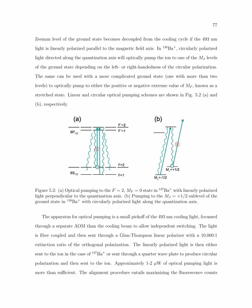
77
Zeeman level of the ground state becomes decoupled from the cooling cycle if the 493 nm
light is linearly polarized parallel to the magnetic field axis. In 138Ba+, circularly polarized
light directed along the quantization axis will optically pump the ion to one of the MJ levels
of the ground state depending on the left- or right-handedness of the circular polarization.
The same can be used with a more complicated ground state (one with more than two
levels) to optically pump to either the positive or negative extreme value of MF , known as a
stretched state. Linear and circular optical pumping schemes are shown in Fig. 5.2 (a) and
(b), respectively.
Figure 5.2: (a) Optical pumping to the F = 2, MF = 0 state in 137Ba+ with linearly polarizedlight perpendicular to the quantization axis. (b) Pumping to the MJ = +1/2 sublevel of theground state in 138Ba+ with circularly polarized light along the quantization axis.
The apparatus for optical pumping is a small pickoff of the 493 nm cooling light, focussed
through a separate AOM than the cooling beam to allow independent switching. The light
is fiber coupled and then sent through a Glan-Thompson linear polarizer with a 10,000:1
extinction ratio of the orthogonal polarization. The linearly polarized light is then either
sent to the ion in the case of 137Ba+ or sent through a quarter wave plate to produce circular
polarization and then sent to the ion. Approximately 1-2 µW of optical pumping light is
more than sufficient. The alignment procedure entails maximizing the fluorescence counts

78
from the ion with the optical pumping beam in an elliptical polarization, which will cool
the ion just as before. By rotating the waveplate to a location which perfectly circularly
polarizes the light, the ion fluorescence will be minimized since the ion can no longer scatter
photons. Of course, the polarization is not perfect and can actually be quantified by a
parameter σ ≡ E+ − E−E+ + E−
, where E+ and E− are the left and right circular components of
the field. Optical pumping efficiency of approximately 90-95% has been observed, measured
by using electron shelving of one of the Zeeman levels. During experiments, the ion is cooled
with elliptically polarized 493 nm light and repumped with 650 nm light. The cooling light
is shut off, but the repump remains on, as the ion still has a probability to decay to the
5D3/2 state during optical pumping. The circularly polarized optical pumping beam is then
switched on for 100-200 µs and then after a short delay the red laser is switched off, leaving
the ion prepared in one of the Zeeman levels.
Of course as mentioned before, the efficiency of circularly polarized optical pumping
depends on the purity of the polarization σ, but also on the alignment of the beam with
the magnetic field axis. The main field coil provides the magnetic field, but separate coils
on the other two perpendicular axes carrying 100-200 mA serve to cancel stray fields at the
trap center and better orient the magnetic field with the pumping beam. These currents are
adjusted to maximize the shelving efficiency to one of the Zeeman levels. If θ is the angle
between the magnetic field and beam’s direction , the optical pumping efficiency is found to
be
P
(MJ =
1
2
)=
1
2+
2σ cos θ
3 + 2σ2 − cos 2θ(5.12)
[58]. This in principle leads to a two-parameter contour of optical pumping as a function of
vertical and horizontal steering coil currents, with what is found to be a broad maximum.
Since it is such a weak dependence and producing this contour is very time consuming,
79
in practice it has been found that simply minimizing PMT counts with a long exposure
while exposing the ion to the optical pumping and red lasers serves as a sufficiently accurate
method to align the field and optical pumping beam.
5.3 Shelving to 5D5/2 at 1.762 µm
The last of the DiVincenzo criteria [28] to receive attention in this work (after the ability
to couple to flying qubits, photons, initialize the qubits by optical pumping and perform
operations with radiation resonant with the frequency splitting between |0〉 and |1〉 states)
is the ability to read out the final qubit state. In this case, the task is accomplished by
state-selectively “shelving” the qubit to the 5D5/2 state, taking it out of the cooling cycle so
it no longer fluoresces, a state detection method pioneered by Dehmelt in the early days of
ion trapping [76].
The laser used for this is a Koheras AdjustikTM thulium-doped fiber laser at 1.762 µm
frequency stabilized via a Pound-Drever-Hall locking scheme to a high-finesse temperature-
controlled ZerodurTM enclosed in vacuum. The frequency stability requirements for this laser
are far more strict than for the ionization and cooling lasers, as it must be able to state-
selectively excite the narrow quadrupole transition from the ground state to 5D5/2 and do so
repeatably. The cavity itself has a free spectral range of about 0.5 GHz and a finesse of 1000,
so a linewidth of 500 kHz. The laser frequency is offset from cavity lines by a double-pass
AOM tunable from 80 to 120 MHz, frequency modulated at 1 MHz with an I/Q modulator
to generate the error signal for the PDH lock servo, which itself is similar to the PDH servo
for the cooling laser doubling cavity. Considerably more detail can be found in [25, 27]. The
portion of the light not sent to the cavity is sent to a second single-pass AOM, where the
first diffracted order is sent to the ion. This AOM has a bandwidth equal to that of the first
and can be scanned to perform high-precision spectroscopy on the 6S1/2 → 5D5/2 transition.

80
With the available laser intensity at the ion, a Rabi frequency of order approximately 100
kHz is achievable.
From measurements of the widths of transitions measured while performing spectroscopy
on the S → D transition, typical widths of 50 kHz are observed. Optical Rabi oscillations
taken on resonance display coherence times greater than 200 µs, indicating a laser linewidth
of about 10 kHz. Because there are many other decoherence sources not related to the
Figure 5.3: Scans of 1.762 µm laser single pass AOM frequency with (black) and without(red) optical pumping at main coil current of 3.0 A. Without optical pumping both MJ
levels of the ground state are equally populated and as a result, the maximum value forthe probability that the ion is dark after shelving one of the Zeeman levels is 50%. Whenoptically pumped, the probability is enhanced for spin up and suppressed for spin down.This plot shows that the two transitions observed without optical pumping originate fromopposite Zeeman levels of the ground state.

81
laser (fluctuating magnetic fields, ion temperature, etc.) this can be taken as an upper
estimate of the linewidth of shelving laser, although there is some reason to suspect from
adiabatic passage experiments, wherein the laser frequency is quickly swept over an atomic
resonance rather than stabilized at the top of it for a fixed exposure, that the stability is
considerably higher [78]. Long term stability, mostly dominated by thermal effects, is also
quite good - observed to be less than 60 mK over the course of three months [27]. This
is mostly dominated by the temperature coefficients of reference voltages and resistors in
the temperature controller and could be improved upon by thermally insulating or even
controlling the electronics, but the level of stability has been found to be sufficient.
Spectroscopy on the transitions amongst Zeeman levels from the ground state to the
5D5/2 state can then be performed similarly to the indirect shelving with the Ti:Sapphire
laser through the 6P3/2 state. The ion is cooled with both the 493 and 650 nm lasers. The
493 nm cooling light is switched off to prevent power broadening of the ground state while
driving the 6S1/2 ↔ 5D5/2 transition, which would otherwise wash out the fine features of
the transition. Delaying turning off the 650 nm light pumps the ion to the ground state,
during which time optical pumping light may or may not be applied to reach a definite
Zeeman level of the ground state. The 1.762 µm light is then switched on for 20 µs to
drive the 6S1/2 → 5D5/2 transition. This pulse is triggered at a fixed value of the phase of
the AC wall voltage to reduce fluctuation due to magnetic perturbations. The duration of
the pulse is chosen to be approximately a π Rabi rotation between the ground and excited
state for carrier transitions and lower order micromotion sidebands, while suppressing the
excitation of weaker sideband transitions. After the pulse is applied, the cooling lasers are
switched on and the ion’s state is determined by observing its fluorescence on the PMT. The
sequence is repeated 40 to 100 times for each value of the shift AOM to accumulate statistics.
Shelving events (when the ion is in a dark state after the fiber laser pulse) are counted and
the frequency of the laser shifted by the single-pass AOM to obtain the desired spectrum. A

82
section of the spectrum performed once with optical pumping and once without is shown in
Fig. 5.3, from which it is obvious the effect that optical pumping has on the spectrum. The
feature at approximately 94.5 MHz is a ∆MJ = +1 transition from the MJ = −1/2 Zeeman
level of the ground state, and the feature at 93.5 MHz is a sideband of the ∆MJ = −1
transition from the opposite MJ level of the ground state. By optically pumping to the spin
down level, the strength of the feature from that level increases from 50% to a maximum
limited by the alignment of the magnetic field with the optical pumping beam axis, while
the other feature is nearly extinguished because that Zeeman state is depopulated.
After locating individual Zeeman transitions through spectroscopy, optical Rabi oscil-
lations can be executed by fixing the AOM frequency to be at the top of a resonance and
varying the pulse length of the 1.762 µm exposure. A typical example can be seen in Fig. 5.4,
taken on the ∆M = +1 from MJ = +1/2 transition. In this way, transitions on micromo-
tion sidebands can be differentiated from those on the carrier transitions. The micromotion
sideband Rabi frequency is supposed by a factor |C±2n|, which is of order one-third for our
trap (refer to Section 2.3 on ion interactions with the trapping field) and hence micromotion
transitions will always be separated by the ΩRF and oscillate more slowly than carriers.
5.4 Precise measurement of g5D5/2
Just as Rabi oscillations with a Ti:Sapphire laser tuned to the 6S1/2 → 6P3/2 transition
provided a means by which to measure all three branching ratios and hence reduced matrix
elements for decays from that state, narrow band excitation to the 5D5/2 state in a magnetic
field provides an opportunity to precisely measure the Lande gJ factor for that state. Prior to
the work presented here and in [59], this quantity was only known from archaic astronomical
observations of line splittings and quoted as 1.12 [73, 5, 22, 74], which is a suspiciously large
deviation from what is expected from L− S coupling (i. e. 6/5=1.2), much larger than any

83
of the other low-lying states in Ba+ (Table 5.1).
The experimental procedure for producing the spectra needed to determine the gJ factor
has been described in the previous section. Scanning the entire range of the single-pass
AOM (80-120 MHz) encompasses either carriers or micromotion sidebands of four different
Zeeman sublevel transitions. Starting at a magnetic field coil current of 3.0 Amps and
progressively decreasing its strength reveals that the spectral resonances converge to several
different values at zero current, where all transitions are degenerate up to separations equal
0 50 100 150 200
0.0
0.2
0.4
0.6
0.8
1.0
Da
rk fra
ctio
n
Exposure time (µs)
Figure 5.4: Optical Rabi oscillations were used to differentiate carrier transitions from theirmicromotion sidebands; this particular example was taken at 94.43 MHz at a coil currentof 2.1 A on the ∆m = +1 from mJ = +1/2 transition. As shown in Fig. 2.3, the strengthof micromotion sidebands is suppressed and hence the Rabi frequency is lower compared tothe carrier transitions. The red line is a fit to an exponentially decaying sine function, thedecay arising from decoherence of the qubit states due to combination of magnetic noise,laser frequency noise and ion temperature.

84
to ΩRF , the separation of micromotion sidebands from their respective carriers. Spectra
were recorded at six different current values - 3.0, 2.6, 2.35, 2.1, 1.6 and 1.0 Amps. The
data are presented in Fig. 5.5 along with lines tracing each of the transitions observed.
By performing spectroscopy without optical pumping, all transitions are visible. Going back
over the spectra with optical pumping reveals from which ground state Zeeman sublevel each
line originates. Referring yet again to the geometry of the quadrupole radiation patterns
shown in Fig. 1.4(b), it can be seen that there is a node in the intensity along the equatorial
plane of the ∆MJ = 0 plot. This is the direction from which the 1.762 µm light is directed
into the trap chamber, so it is immediately apparent that only ∆MJ = ±1 or ±2 transitions
are driven, the latter more strongly than the former.
Now the task remains to interpret the resulting spectra. The basic idea is to determine
the expected relative positions of the different transitions in Fig. 5.1 as the magnetic field
varies. Of the lines observed, two pairs are found to translate parallel to one another along
the entire range of currents measured. Moreover, they are always separated by exactly the
trap frequency ΩRF , so they can immediately be identified as carrier transition/micromotion
sideband pairs. The Rabi frequency of optical rotations between the ground and excited
state on each line reveal that the stronger line is the carrier and the weaker the sideband.
Carrier transitions have typical π rotation times of 10 µs, while sidebands require 20-30 µs.
Two weaker transitions are found to converge to a zero current frequency 12.38 MHz above
that of the first-order micromotion sidebands. This is consistent with them being second-
order micromotion sidebands of two other transitions outside of the range accessible with the
single-pass AOM. The error in bright vs. dark counts is taken to be binomial and each peak is
fit to a three-parameter Lorentzian profile Pdark(ω) = 1π
A(ω − ωc)2 + γ2 , where the parameter
of interest is the central frequency of the transition ωc. Typical statistical uncertainty in the
fit of this parameter is of order several kHz. From the separations of seven measured pairs
of carrier transitions/micromotion sideband pairs, the trap frequency can be determined to

85
Figure 5.5: (a) All spectra measured without optical pumping showing 6S1/2 ↔ 5D5/2 tran-sitions at six different values for the main coil current. The lines on the figure are inserted byhand to guide the eye. Resonances not crossed by the guiding lines were identified as secularsidebands by their characteristic frequency separation from main transitions. The dashed,yellow lines are the ∆M = +1 from MJ = +1/2 and its 1st order micromotion sideband, thesolid, red lines are the ∆M = −1 from MJ = −1/2 and its 1st order micromotion sidebandand dash-dot, green the 2nd order sidebands of ∆M = −2 from MJ = −1/2 and ∆m = −1from mJ = +1/2. Secular motion sidebands at 2.5, 1.4 and 0.6 MHz are visible as well butdeliberately not emphasized by added lines (b) A representative spectrum taken withoutoptical pumping at 2.1 Amps. Arrow line styles (colors) correspond to the same schemeused to label transitions in (a).
be ΩRF = 12.3759 ± 0.0025 MHz. By subtracting the measured trap frequency from first
order micromotion sidebands and twice that frequency from second order sideband positions,
we calculate the position of the carrier frequency for four Zeeman transitions: ∆MJ = +1
from∣∣6S1/2 ; MJ = +1/2〉, ∆MJ = −1 from
∣∣6S1/2 ; MJ = −1/2〉, ∆MJ = −1 from∣∣6S1/2 ;
MJ = +1/2〉 and ∆MJ = −2 from∣∣6S1/2 ; MJ = −1/2〉 (see Fig. 5.6).
From the extrapolated peak positions, one can take the zero field 6S1/2 → 5D5/2 transition
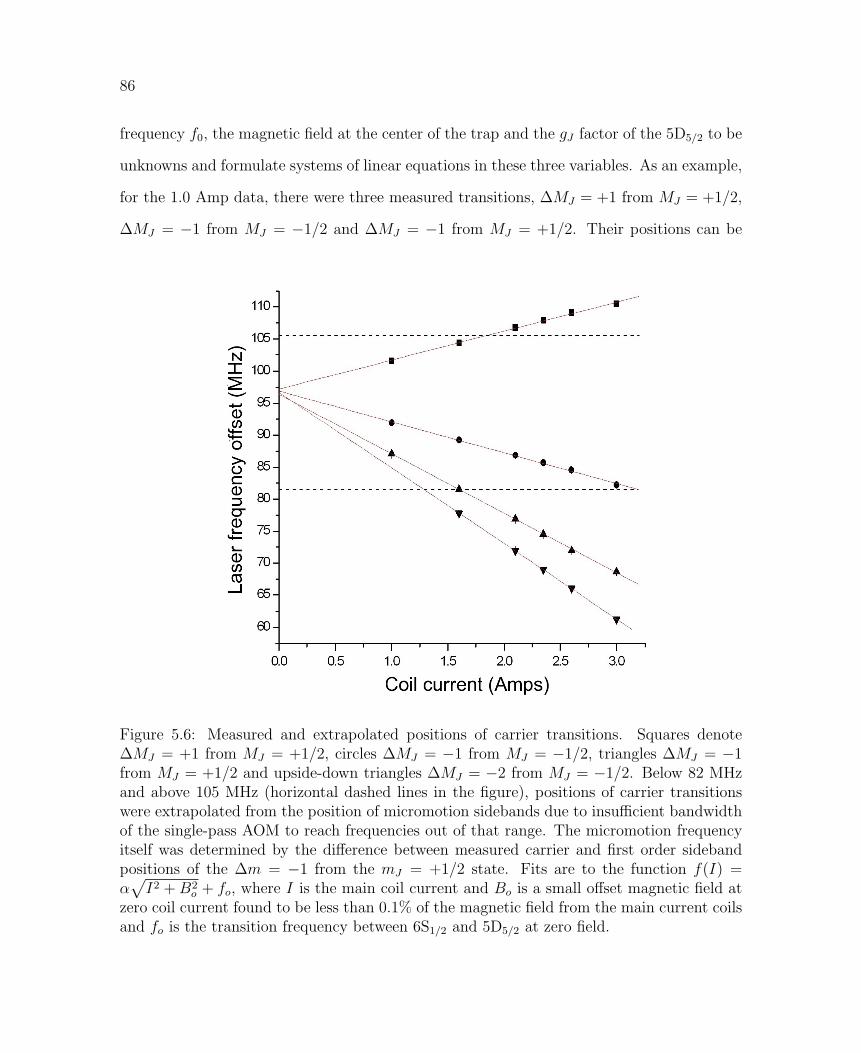
86
frequency f0, the magnetic field at the center of the trap and the gJ factor of the 5D5/2 to be
unknowns and formulate systems of linear equations in these three variables. As an example,
for the 1.0 Amp data, there were three measured transitions, ∆MJ = +1 from MJ = +1/2,
∆MJ = −1 from MJ = −1/2 and ∆MJ = −1 from MJ = +1/2. Their positions can be
Figure 5.6: Measured and extrapolated positions of carrier transitions. Squares denote∆MJ = +1 from MJ = +1/2, circles ∆MJ = −1 from MJ = −1/2, triangles ∆MJ = −1from MJ = +1/2 and upside-down triangles ∆MJ = −2 from MJ = −1/2. Below 82 MHzand above 105 MHz (horizontal dashed lines in the figure), positions of carrier transitionswere extrapolated from the position of micromotion sidebands due to insufficient bandwidthof the single-pass AOM to reach frequencies out of that range. The micromotion frequencyitself was determined by the difference between measured carrier and first order sidebandpositions of the ∆m = −1 from the mJ = +1/2 state. Fits are to the function f(I) =α√I2 +B2
o + fo, where I is the main coil current and Bo is a small offset magnetic field atzero coil current found to be less than 0.1% of the magnetic field from the main current coilsand fo is the transition frequency between 6S1/2 and 5D5/2 at zero field.

87
calculated from the standard formula for Zeeman shift (Eq. 5.3)
f1 − f0 =µBB
2~(3gD − gS)
f2 − f0 =µBB
2~(−3gD + gS)
f3 − f0 =µBB
2~(−gD − gS) (5.13)
The variables f0 and B can be eliminated by pairwise summing the equations and taking a
ratio of the remaining two combined equations. This has the additional advantage that only
frequency differences and no absolute frequencies are required, cutting down on the possible
systematic errors which would otherwise be incorporated into the determination of the g
factor. The final algebraic expression which must be solved is then
f1 − f2
f3 − f2
=3gD/gS − 1
gD/gS − 1(5.14)
For all other current values, there is an additional transition, ∆MJ = −2 from MJ = −1/2,
which actually overdetermines the system of equations adding f4 − f0 =µBB2~ (−5gD + gS).
Two values for the g factor ratio gD/gS can be found from the data and they are found to
agree well within the statistical uncertainty. Using the measured value for gS from Table
5.1, 2.0024906(11) [56], the absolute value for g5D5/2can be found to be 1.2020 ± 0.0005.
The prediction from strict L − S coupling is 6/5, the difference arising from leading order
QED shifts including electron self-energy and vacuum polarization, interactions between the
valence electron and core shell as well as relativistic effects. The largest corrections occur
at the α (αZ)2 level, approximately where the deviation from 6/5 is observed here [55, 46].
Going back to the system of linear equations used to calculate the g factor, the magnetic
field at the center of the trap can be found to be 0.067 mT per Amp of current applied to

88
the main field coils, a value that will be useful when attempting to drive Rabi oscillations
between the two MJ Zeeman levels of the ground state with the magnetic dipole component
of incident RF radiation as described earlier in this chapter.
There are several sources of systematic error. There is no concern over linewidths or
transition strengths, so only effects that influence the relative frequencies of transitions in an
individual run need to be considered. Two sources of error related to trapping parameters are
the variation of the ion’s position with respect to the magnetic field and AC Zeeman shifts
caused by currents induced in the trap by the high RF voltages. An estimate of the former
is at the levels of 10−4 as the ion’s position varies by much less than a few microns over the
course of the experiment, as observed on a electron-multiplied CCD camera, and magnetic
gradients are of the order 40 nT/µm. AC Zeeman shifts have been seen to affect g factor
measurements, albeit at the 10−4 level in slightly different trap geometries [94], but these are
highly suppressed in our trap design because of the large distance between the ion and the
nearest grounded electrode through which current is able to pass to ground. Several potential
sources of frequency error are related to the shelving laser itself. Drifts can occur both on
the locking cavity due to pressure or temperature variations and in the phase of the 60 Hz
AC voltage to which the beginning of the shelving pulse is triggered. This is only a problem
during the course of a single run at each individual magnetic field, since the extraction of
the g factor comes from each field value rather than a fit as a function of field. One can use
the observed change in the position of the 6S1/2 → 5D5/2 transition as a combined measure
of these effects. The central (non Zeeman-shifted) value for the 6S1/2 → 5D5/2 transition
lies midway between the ∆MJ = +1 from∣∣6S1/2 ; MJ = −1/2〉 and ∆MJ = −1 from
∣∣6S1/2 ;
MJ = +1/2〉 transitions. This value agrees to within 4 kHz for the different values of coil
current. From this uncertainty, a worst estimate of the shift over the course of an individual
run, which is at most one hour in duration, is a few kHz. This represents the dominant
contribution to the systematic uncertainty and the overall systematic error in the g factor

89
measurement can be assumed to be ±0.0001.

90

6 TOWARD A ZEEMAN QUBIT & OUT-
LOOK
Schnee und Sturm und Felsgestein
Stahlt den Fuß und ubt das Bein.
Immer hinterm Offen sein,
macht das Leben arm und klein
-Gunnar Gunnarsson
I’ve had a good time. This just wasn’t it.
-Graucho Marx
Up until now, there has been very little motivation for the experiments presented in the
chapters leading up to here, seemingly violating the mantra, “say what you are going to say,
say it and then review it.” This, however, was not done without purpose. Perhaps it was a bit
of historical perspective on the work presented, since it more or less chronologically follows
the progression of what was done. Along those same lines, perhaps the reason for only a
vague sense of the exact methods and applications was to recreate some of the sentiment of
the author, for whom the path to entanglement was not always so clear. Maybe it was to give
the reader the opportunity to think about the utility of the methods presented here for him or
herself. Whatever the reason, the intent in this final chapter is to wrap everything together
into a single (incomplete) set of experiments aimed at realizing several goals in practical
91
92
quantum computation as well as a few foundational aspects of studying quantum mechanics.
The two broad categories are less separate than the previous sentence might imply, but I
hesitate to use the word “practical” with the foundations of quantum mechanics, as it may
be difficult to impress upon, say the person sitting next to you on the bus, the burdensome
importance of simultaneously closing all of the local loopholes in a Bell’s inequality test.
6.1 Zeeman qubit: How & why?
Referring to Fig. 3.8 one finds two ion-photon entanglement schemes - a frequency qubit at
493 nm in 137Ba+ and a polarization qubit in 138Ba+. As already noted in the text associated
with the figure, neither of these qubit schemes represents a particularly good way in which
to entangle ion spin with photon modes. A polarization qubit has the advantage of having
straightforward qubit rotations by simply rotating a half-wave plate and not experiencing any
chromatic dispersion through optics and optical fiber. A frequency qubit has the advantage
that any optical process which disturbs polarization, such as reflections from curved surfaces
and propagation through optical fiber will not mix the qubit states. This allows a greater
collection angle than that for a polarization qubit, since the error rate due to mixing of
polarizations from the two radiation patterns for dipole radiation (Fig. 1.4(a)) is proportional
to the square of the solid angle subtended by the collection optics, ∝ (∆Ω)2.
It has already been alluded to, but the ionic qubit of choice is one encoded in the Zeeman
levels of the 6S1/2. While there are many advantages to using 137Ba+ and exploiting its
hyperfine levels to make magnetically insensitive qubit levels, the nuclear spin of 3/2 creates
very complex state manifolds even in the ground state. Operating a Ti:Sapphire on resonance
with the 6S1/2 → 6P1/2 transition at 493 nm offers some hope of generating ion-photon
entanglement looking only at ∆MF = 0 transitions using the selection rule that such decays
must change the F quantum number, but this ignores all decay channels for which ∆MF =

93
±1, or two-thirds of the total decays. Any decay from one of the stretched states (the only
other states to which the ion can be initialized via optical pumping where one could envision
generating a polarization qubit on decay) will generate at least one unwanted decay. Looking
to the 6P3/2 state is even more hopeless, since there are four F levels all of which fall into
the bandwidth of the 400 fs pulses from the Ti:Sapphire laser. It is therefore desirable to
work instead with a spin-12 system, 138Ba+.
A possible objection to this proposal is that there are no magnetically insensitive levels
in 138Ba+, so decoherence of the ionic qubit due to magnetic noise will render this ion-
photon entanglement generation scheme useless. Such a qubit scheme has been implemented
with 88Sr+ ions [23]. Moreover, looking at the several hundred microsecond coherence time
of optical Rabi oscillations gives some idea of an upper limit of how fast the qubit states
decohere due to magnetic noise. Since the photon travel time is a negligible fraction of this
time, there will be no degradation of the fidelity during the time operation are performed
on the photonic qubit. While applying 8 Ghz radiation to 137Ba+ must be performed with a
microwave horn mounted outside the trap chamber such that no focussing of the radiation is
possible, the tens of MHz RF radiation needed to drive qubit rotations can be applied directly
to the trap electrodes, potentially making qubit rotations very fast. Even greater speed and
improved insensitivity to magnetic fluctuations would be possible if qubit operations were
performed with a pair of Raman beams. Moreover, line-triggering of experimental sequences,
magnetic shielding and perhaps active field compensation can be employed to further extend
the coherence time which has already been observed. Detection with adiabatic passage by
sweeping the 1.762 µm laser over the desired qubit level rather than fixing the frequency
of the laser at the atomic resonance has improved fidelity of detection even with a slightly
varying magnetic field.
The greatest advantage of the proposed Zeeman qubit is its simplicity. Generation
of ion-photon entangled states simply requires optically pumping with σ+ polarized light

94
in a manner identical to that employed in the g factor measurement presented in the
previous chapter. A single π polarized femtosecond pulse at 493 nm will excite the ion
to the same Zeeman sublevel in the 6P1/2 pair of states. On decay the entangled state
1√2
(|MJ = +1/2;π〉+ |MJ = −1/2;σ〉) will be created. Qubit states are separated by a
splitting determined by the magnetic field, which has already been found to equal 0.067
mT/A or applied coil current or, using the measured g6S1/2= 2.0024906, 12.4 MHz/A. The
small splitting and the fact that the transition is magnetic dipole means these states are
extremely long-lived. Qubit rotations are performed applying RF modulation to the ground
electrodes in the trap which are shorted on the side opposite the helical resonator. This has
been described in Section 5.1 where it was assumed that the oscillating magnetic field was
directed perpendicular to the quantization axis and had a ±1 helicity component. Since the
ion is at the center of where the driving field originates, the near-field form of the oscillating
magnetic field will have all three “polarization” components to drive the magnetic transition.
The sequence of experiments leading to the demonstration of a Zeeman qubit is to first
perform 1.762 µm spectroscopy as described in the previous chapter to locate a resonance
from the optically pumped state to the 5D5/2 state for detection. Once such a resonance
is located, RF spectroscopy must be performed to locate the resonance between the two
Zeeman levels. RF radiation is synthesized by a Stanford Research Systems DS345 function
generator at -20 dBm, amplified to +22 dBm and sent directly to the ground electrodes of
the trap, accessed on the output end of the helical resonator. After optically pumping the ion
to the bright qubit state, all lasers are shut off and a 50 µs pulse of RF radiation is applied
to attempt to drive the ion into the opposite Zeeman level. This was found to heat the ion
significantly, presumably because the frequency is very nearly twice the trap frequency. Since
shelving efficiency depends strongly on ion temperature, performing state detection with a
fixed duration, fixed frequency 1.762 µm pulse failed miserably. Instead, this was a perfect
opportunity to employ the pulse sequencer described in section 2.4; shelving pulses were

95
replaced by frequency ramps over a fixed range at a rate chosen to adaibatically transfer ion
population from the ground to the excited state. This is a much more robust shelving method,
displaying significantly better insensitivity to ion temperature and magnetic fluctuations.
Preliminary results of RF spectroscopy are shown in Fig. 6.1.
Figure 6.1: Preliminary results for driving RF Zeeman transitions between the 6S1/2;MJ =±1/2 levels in 138Ba+. The flat shelving level at 85% represents the maximum opticalpumping/adiabatic passage shelving efficiency achieved. If the observed dip represented a πpulse, it would ostensibly reach approximately 15%. However, there is no reason to assumethat the transition was not over- or under-driven, either of which would result in less thanunit efficient population transfer.
6.2 From entangled ions and photons to entangled ions
The real utility of generating entangled ion-photon pairs is to transmit information about
the quantum state of the ion over long distances to other ions. Several schemes have been
proposed to accomplish this task [15, 99, 30]. The first such scheme involves weakly exciting
the ion from the ground |↓〉 state to a metastable excited state |e〉 with probability ε
1. The excited state has equal probability to decay to |↓〉 or |↑〉, and the detectors are

96
sensitive only to the latter. So after excitation of both ions, the state is (|↓〉1 +√ε |e〉1) ⊗
(|↓〉2 +√ε |e〉2). Conditioned on detection of a |e〉 → |↑〉 photon, the ions will be projected
into the state 1√2
(|↓〉1 |↑〉2 + eik∆x ↑〉1 |↓〉2
)after a 50-50 beam splitter. This scheme suffers
from the probability of multiple excitations and the fact that the relative phase caused by
any optical path length difference ∆x will ruin the entanglement fidelity. The second scheme
requires the detection of coincident pairs of photons, so suffers from lower entanglement
generation rate, but is much more robust. Experimentally the second scheme has been
achieved with Ytterbium ions [72], but the emitted photons in that case are at a wavelength
of 369 nm. This is UV and hence limits the distance over which the photons propagate in
single-mode optical fiber to a few meters at most. As mentioned before, Ba+ emits at 493
nm, so the emitted photons experience significantly less attenuation, enabling both a higher
repetition rate for successful generation of entangled pairs of ions as well as longer distance
between ions.
If a pair of 138Ba+ ions is optically pumped to the spin up MJ = +1/2 Zeeman level of
the 6S1/2 state, which will hereafter be denoted as |↑〉, and excited with a linearly polarized
pulse from a Ti:Sapphire laser to the spin up state in the 6P1/2 state, there are no mixings of
levels on the excitation. Likewise on decay, each ion has two possible decay channels, each
of which is equally likely, so the state of the two ions after several P state lifetimes (tens of
ns) is
|Ψ〉 =1
2(|↑1〉 |π1〉+ |↓1〉 |σ1〉)⊗ (|↑2〉 |π2〉+ |↓2〉 |σ2〉)
=1
4[(|↑1↑2〉+ |↓1↓2〉)⊗ (|V1V2〉+ |H1H2〉)
+ (|↑1↑2〉 − |↓1↓2〉)⊗ (|V1V2〉 − |H1H2〉)
+ (|↑1↓2〉+ |↓1↑2〉)⊗ (|V1H2〉+ |H1V2〉)

97
+ (|↑1↓2〉 − |↓1↑2〉)⊗ (|V1H2〉 − |H1V2〉)] (6.1)
where it has been identified that if the ion is observed perpendicular to the quantization axis
that the π and σ decay modes are orthogonal and correspond to vertically and horizontally
polarized photons, respectively. This isn’t interesting yet, since the two ion-photon pairs are
in a product state. If the two emitted photons are matched temporally and spatially on a
50-50 non-polarizing beam splitter as described in section 4.1 for the case of a single photon,
the interference between the two amplitudes for both photons being transmitted or both be-
ing reflected can project the ions into an entangled state by removing which-way information
from each individual photon as described in Chapter 4. Because of the antisymmetrization of
the overall wavefunction [52], the two photons will emerge from different output ports of the
beam splitter only if they are in the state 1√2
(|V1H2〉 − |H1V2〉), immediately heralding the
ion-ion state 1√2
(|↑1↓2〉 − |↓1↑2〉). With polarizing beam splitters located in each of the out-
put channels and four PMT’s, it is possible to detect the photon state 1√2
(|V1H2〉+ |H1V2〉)
and generate the symmetric state 1√2
(|↑1↓2〉+ |↓1↑2〉). Detecting two photons in the same
output port corresponds to the 1√2
(|V1V2〉 ± |H1H2〉) states and does not generate a unique
ion-ion entangled state [71].
This is a probabilistic process because only a very small percentage of the decays actually
results in an entangled pair. There is effort to enclose each ion in an optical cavity to
preferentially emit into a single spatial mode thereby making the process nearly deterministic
[105, 7]. The probability for successful ion-photon entanglement generation is Pion−ph =
PexcBI∆Ω
(∆Ω4π
)Tη, where Pexc is the probability of excitation, B the branching ratio to the
desired qubit states, I∆Ω the intensity of the radiation into the solid angle of collection ∆Ω,
T the loss due to transmission through optical fiber or from other optical elements such as
interference filters and η the single-photon detection efficiency. Since two such single photon
events are necessary for the generation of entangled ion pairs and only one of four Bell states
98
is detected from the post-selection process described above, the probability for success in that
case is Pion−ion = 14P
2ion−ph. The use of mode-locked pulses for excitation enables Pexc ≈ 1
and using long wavelength transitions ensure that T and η are as high as possible. Additional
sensitivity may be gained by using avalanche photodiodes (APD’s) for detection rather than
PMT’s which would have a quantum efficiency closer to 80% rather than 10-20%. The
greatest gains in efficiency come from improving the solid angle ∆Ω from which photons are
collected, which even with the best refractive optics available is typically only a few percent
of the sphere [6] because of the distance between the ions and vacuum viewports. Several
schemes using in-vacuum parabolic [69] and spherical mirrors with downstream aspherical
correctors [97] have been investigated to boost fluorescence collection significantly. If ion
state detection, the speed bottle-neck of the entire pulse sequence required, is conditioned
on detection of a photon, the experiment can be run at a high repetition rate, perhaps a few
kHz. Even still, an entanglement generation probability of a few times 10−8 is the current
state of the art [72]. Construction of a partial Bell state analyzer (i. e. one that only
generated the antisymmetric Bell state) has begun in our lab, using Toptica FiberDocksTM
with identical triplet lenses as the outputs of two single-mode optical fibers, each directed
onto a 50-50 beam splitter at as near normal incidence as possible. A half wave plate on a
rotation mount in one arm of the interferometer can be rotated to change the measurement
basis. The entire apparatus is enclosed in a light-tight box to keep error du to background
counts at a minimum. Optical elements are mounted on remote-controllable Pico-motorTM
mounts.
6.3 Applications
There are several applications of heralded entangled states of ions remotely separated by as
great a distance as the ≤ 30 dB/km attenuation of 493 nm photons in optical fiber allows.

99
Since the Zeeman or hyperfine states involved have nearly infinite decay times, the entangled
state can be pre-prepared for delayed measurement.
Entangled pairs of particles have long been used to test the famous Bell’s inequality [8].
The generic Gedankenexperiment, recast in the more experimentally friendly CHSH form,
proceeds as follows. At two different locations A and B, so labelled to reflect the identity
of the experimenters Alice and Bob, two different measurements A(a) or A(a′) and B(b) or
B(b′) can be performed. The combination of correlations C
S ≡ C[A(a), B(b)] + C[A(a), B(b′)] + C[A(a′), B(b)]− C[A(a′), B(b′)] (6.2)
can be measured. In the case of classical systems, where the values of each measurement
are uncorrelated and can take the values ±1, either B(b)±B(b′) will be zero and the other
equal to two. So the average of many such experiments performed on the system will lead to
S ≤ 2, which is the Bell inequality. For a quantum mechanical system, if the measurements
are the values of some non-commuting pair of operators such as two different components
of a particle’s spin along a different set of coordinate axes at each location A and B, the
expectation value
S =
⟨particle 1︷︸︸︷−σz ·
1√2
(σz + σx)︸ ︷︷ ︸particle 2
⟩+
⟨σz ·
1√2
(σz − σx)⟩
+
⟨−σz ·
1√2
(σx + σx)
⟩−⟨σx ·
1√2
(σz − σx)⟩
= 2√
2 (6.3)
when the two particles are produced in a Bell state. This is clearly greater than two, violating
Bell’s inequality [18, 19].
An interesting application of remotely generated entangled ion pairs not related to quan-
tum information processing is a Bell’s inequality measurement that simultaneously closes

100
the detection and locality loopholes prognosticated by local hidden variable theories [99].
The former maintains that unless the detection efficiency is high enough (greater than 70%),
the possibility remains that the experiment is biased by the subset of measurements that do
violate the inequality while the greater set of all experiments measured and not measured
do not violate Bell’s inequality. This has actually been closed by trapped ion experiments
[89]. The second loophole, known as the “locality” or “lightcone loophole,” hypothesizes
that subluminal signals can propagate amongst the different parts of the apparatus unless
the choice of basis for measurement is outside of the reverse lightcone of the measurements
on the opposite particle of the Bell pair. This has been closed with entangled photon pairs
[103]. The state detection efficiency in trapped ions can easily be near unity, so the first
Figure 6.2: Adapted from [99], these show the space-time diagram of the progression of aBell’s Inequality test that would simultaneously close the detection and locality loopholes.Left, the partial Bell-state analyzer is midway between the two ion traps, while to the rightis a more likely experimental situation. “Emit” 1 and 2 refer to the ion excitation and decay,where the emitted photon propagates along the world-line at less than c. The entanglementof the ions is created where indicated, and “Choose” 1 and 2 refer to the choice of basis ateach location.

101
loophole is easily closed. The latter can be closed if the experiment is set up as depicted in
the space-time diagram shown in Fig. 6.2, with the ions located in separate traps separated
by a distance of say one mile. The light travel time between the two locations would be
5.3 µs. The velocity of the photons carrying the quantum information from each ion to
the partial Bell state analyzer for the entanglement procedure would be slightly less than c
because of the optical fiber, so the choice of basis for each measurement could fall outside
of the reverse light cone of the opposite ion’s measurement. Although the excitations (a few
hundred femtoseconds) and decays (perhaps 50 ns) are not the bottle-necks, the individual
qubit rotations and detection steps would have to take no more than a few microseconds, a
difficult but in principle attainable feat.
While there is considerable effort in the trapped ion community to make ion traps smaller
and smaller, incorporating increasing numbers of atoms in microfabricated trap structures
capable of shuttling ions along tracks and even turning corners [102, 51], an alternative ap-
proach to a large-scale quantum computer is to employ what has been known as a cluster
state [32]. In this model, a large-scale entangled array of ions is entangled via multiple
photon-mediated entangling operations as described and the resulting cluster state can be
used to perform quantum computations via appropriately chosen single-qubit projective
measurements. It has been shown to be computationally equivalent to any conventional
quantum circuit model computation so long as the entangled state incorporates two dimen-
sions [87]. This is achieved with several 1D chains generated as already described, connected
by a Hadamard/controlled phase flip operation on two ions in the middle of the entangled
chains. The overhead in terms of the time required to generate the entangled state scales
polynomially with the number of ions required. It is also possible to imagine using this
probabilistic entanglement scheme to create local pairs of entangled ions which can then
be used to implement deterministic gates between different sectors of a large-scale ion trap
array. Quantum repeater schemes where entanglement is passed between intermediate nodes

102
separated by short distance can be used to turn the distance scaling from exponentially to
linearly decaying [14, 31]

Bibliography
[1] Leslie Allen and J. H. Eberly. Optical Resonance and Two-Level Atoms. Dover Publi-cations N. Y., Inc., 1987.
[2] Markus Ansmann et al. Violation of Bell’s inequality in Josephson phase qubits.Nature, 461:504–6, 2009.
[3] O. H. Arroe. Hyperfine structure and isotope shift in barium. Phys. Rev., 79:836,1950.
[4] A. Aspect, P. Graingier, and G. Roger. Experimental realization of the Eintein-Podolsky-Rosen gedankenexperiment: A new violation of Bell’s inequalities. Phys.Rev. Lett., 49:91–4, 1982.
[5] E. Back. Zur Kenntnis des Zeemaneffekts. Annalen der Physik, 375(5):333–372, 1923.
[6] W. S. Bakr, J. I. Gillen, A. Peng, S. Folling, and M. Greiner. A quantum gas microscopefor detecting single atoms in a Hubbard-regime optical lattice. Nature, 462:74–77, 2009.
[7] H. G. Barros, A. Stute, T. E. Northup, C. Russo, P. O. Schmidt, and R. Blatt. De-terministic single-photon source from a single ion. New Jour. of Phys., 11:103004,2009.
[8] J. S. Bell. On the problem of hidden variables in quantum mechanics. Reviews ofModern Physics, 38:447, 1966.
[9] K. Beloy, A. Derevianko, V. A. Dzuba, G. T. Howell, B. B. Blinov, and E. N. Fortson.Nuclear magnetic octupole moment and hyperfine structure of the 5D3/2,5/2 states ofthe Ba+ ion. Phys. Rev. A, 77:052503, 2008.
[10] D. Berkeland, J. D. Miller, J. Bergquist, W. M. Itano, and D. J. Wineland. Minimiza-tion of micromotion in a linear Paul trap. Jour. of App. Phys., 83:5025–33, 1998.
[11] D. J. Berkeland and M. Boshier. Destabilization of dark states and optical spectroscopyin Zeeman-degenerate atomic systems. Phys. Rev. A, 65:33413, 2002.
103

104
[12] Eric Black. Notes on the Pound-Drever-Hall technique. Technical Report LIGO-T980045-00-D, Laser Interferometry Gravitational Wave Observatory, California Insti-tute of Technology, 1998.
[13] R. Blatt and D. J. Wineland. Entangled states of trapped atomic ions. Nature,453:1008–1014, 2008.
[14] H. J. Briegel, W. Duer, J. I. Cirac, and P. Zoller. Quantum repeaters: The role ofimperfect local operations in quantum communitation. Phys. Rev. Lett., 81:5932–5,1998.
[15] C. Cabrillo, J. I. Cirac, P. Garcıa-Fernandez, and P. Zoller. Creation of entangled stateof distant atoms by interference. Phys. Rev. A, 59:1025–33, 1999.
[16] W. C. Campbell et al. Ultrafast gates for single atomic qubits. Phys. Rev. Lett.,105:090502, 2010.
[17] J. I. Cirac and P. Zoller. Quantum computations with cold trapped ions. Phys. Rev.Lett., 74:4091–4, 1995.
[18] J. F. Clauser and M. A. Horne. Experimental consequences of objective local theories.Physical Review D, 10:526–35, 1974.
[19] J. F. Clauser, M. A. Horne, A. Shimony, and R. A. Holt. Proposed experiment to testlocal hidden-variable theories. Physical Review Letters, 23:880–4, 1969.
[20] Coherent Laser Group, Santa Clara, CA. The Coherent Mira model 900-B laser, 1993.
[21] T. B. Coplen et al. Commission on atomic weights and isotopic abundances report forthe International Union of Pure and Applied Chemistry. In Isotopic Compositions ofthe Elements, volume 70, page 217. IUPAC, 1998.
[22] J. J. Curry. Barium g factors. Jour. Phys. Chem. Ref. Data, 33:725, 2004.
[23] Yehonatan Dallal. Toward high fidelity single ion qubit gates. Master’s thesis, Weiz-mann Institute of Science, Rehovot, Israel, 2009.
[24] H. Dehmelt and P. A. Ekstrom. Proposed 10144ν < ν laser fluorescence spectroscopyon Tl+ mono-ion oscillator. Bull. Am. Phys. Soc., 18:1521, 1973.
[25] M. R. Dietrich and B. B. Blinov. Use of a microcontroller for fast feedback control ofa fiber laser. [arXiv:0905.2484], 2009.
[26] M. R. Dietrich, N. Kurz, T. Noel, Gang Shu, and B. B. Blinov. Hyperfine and opticalbarium qubits. Phys. Rev. A, 81:052328, 2010.
[27] Matthew R. Dietrich. Barium ions for quantum computation. PhD thesis, Universityof Washington, 2009.

105
[28] David DiVincenzo. Quantum computation. Science, 270(5234):255–61, 1995.
[29] L.-M. Duan. Scaling ion trap quantum computation through fast quantum gates. Phys.Rev. Lett., 93:100502–1, 2004.
[30] L.-M. Duan and J. Kimble. Efficient engineering of multi-atom entanglement throughsingle-photon detections. Phys. Rev. Lett., 90:253601, 2003.
[31] L.-M. Duan, M. D. Lukin, J. I. Cirac, and P. Zoller. Long distance quantum commu-nication with atomic ensembles and linear optics. Nature, 414:413–8, 2001.
[32] L.-M. Duan and R. Raussendorf. Efficient quantum computation with probabilisticquantum gates. Phys. Rev. Lett., 95:080503, 2005.
[33] V. A. Dzuba and V. V. Flambaum. Atomic optical clocks and a search for the variationof the fine structure constant. Phys. Rev. A, 61:034502, 2000.
[34] V. A. Dzuba, V. V. Flambaum, and J. S. M. Ginges. Calculations of parity noncon-serving s-d transitions in Cs, Fr, Ba+ and Ra+. Phys. Rev. A, 63:062101, 2001.
[35] V. A. Dzuba and J. S. M. Ginges. Calculations of energy levels and lifetimes of low-lying states of barium and radium. Phys. Rev. A, 73:032503, 2006.
[36] A. R. Edmunds. Angular Momentum in Quantum Mechanics. Princeton UniversityPress, 1960.
[37] A. Einstein, B. Podolsky, and N. Rosen. Can a quantum-mechanical description ofreality be considered complete? Physical Review, 47:777, 1935.
[38] Richard P. Feynman. Simulating physics with computers. Int. Jour. of Theor. Phys.,21:467–88, 1982.
[39] Christopher J. Foot. Atomic Physics. Oxford University Press, 2005.
[40] T. M. Fortier et al. Precision atomic spectroscopy for improved limits on variation ofthe fine structure constant and local position invariance. Phys. Rev. Lett., 98:070801,2007.
[41] E. N. Fortson. Possibility of measuring parity non-conservation with a single trappedatomic ion. Phys. Rev. A, 70:2383–2386, 1993.
[42] S. J. Freedman and J. F. Clauser. Experimental test of local hidden variable theories.Phys. Rev. Lett., 28:938–41, 1972.
[43] A. Gallagher. Oscillator strengths of CaII, SrII and BaII. Phys. Rev., 157:24, 1967.

106
[44] J. J. Garcıa-Ripoll, P. Zoller, and J. I. Cirac. Speed optimized two-qubit gate withlaser coherent control techniques for ion trap quantum computation. Phys. Rev. Lett.,91:157901, 2003.
[45] V. Gerginov. Observation of a nuclear magnetic octupole moment of Cesium-133through high resolution laser spectroscopy. PhD thesis, Notre Dame, 2003.
[46] D. A. Glazov, V. M. Shabaev, I. I. Tupitsyn, A. V. Volotka, V. A. Yerokhin, G. Plunien,and G. Soff. Relativistic and QED corrections to the g factor of Li-like ions. Phys.Rev. A, 70:062104, 2004.
[47] Apollo Go. Observation of Bell inequality violation in B mesons. Jour. of Mod. Optics,51:991–8, 2004.
[48] G. Gopakumar, H. Merlitz, R.K. Chaudhuri, B. P. Das, U. S. Mahapatra, andD. Mukherjee. Electric dipole and quadrupole transition amplitudes for Ba+ usingthe relativistic coupled-cluster method. Phys. Rev. A, 66:032505–1–6, 2002.
[49] C. Guet and W. R. Johnson. Relativistic many-body calculations of transition ratesfor Ca+, Sr+, and Ba+. Phys. Rev. A, 44:1531–5, 1991.
[50] D. Hayes et al. Entanglement of atomic qubits using and optical frequency comb. Phys.Rev. Lett., 104:140501, 2010.
[51] W. K. Hensinger, S. Olmschenk, D. Stick, D. Hucul, M. Yeo, M. Acton, L. Deslauri-ers, C. Monroe, and J. Rabchuk. T-junction ion trap array for two-dimensional ionshuttling, storage and manipulation. Appl. Phys. Lett., 88:034101, 2006.
[52] C. K. Hong, Z. Y. Ou, and L. Mandel. Measurement of subpicosecond time intervalsbetween two photons by interference. Phys. Rev. Lett., 59:2044–6, 1987.
[53] G. Janik, W. Nagourney, and H. Dehmelt. Doppler-free optical spectroscopy on theBa+ mono-ion oscillator. Jour. of the Opt. Soc. of Am. B, 2:1251–7, 1985.
[54] A. Kastberg, P. Villemoes, A. Arnesen, F. Heijkenskjold, A. Langereis, P. Jungner, andS. Linnæus. Measurement of absolute transition probabilities in BaII through opticalnutation. Jour. Opt. Soc. Am. B, 10:1330, 1993.
[55] O. Yu Khetselius. Relativistic calculation of the hyperfine structure parameters forheavy elements and laser detection of the heavy isotopes. Phys. Scr., T135:014023–6,2009.
[56] K. H. Knoll, G. Marx, K. Hubner, F. Schweikert, S. Stahl, C. Weber, and G. Werth.Experimental gJ factor in the metastable 5D3/2 state of Ba+. Phys. Rev. A, 54:1199–1205, 1996.

107
[57] H. Kogelnik and T. Li. Laser beams and resonators. Proceedings of the IEEE, 54:1312–29, 1966.
[58] T. Korber. Measurement of light shift ratios with a single trapped 138Ba+ ion, andprospects for a parity violation experiment. PhD thesis, University of Washington,2003.
[59] N. Kurz, M. R. Dietrich, G. Shu, T. Noel, and B. B. Blinov. Measurement of Landeg-factor of 5D5/2 state of BaII with a single trapped ion. Phys. Rev. A, 82:030501(R),2010.
[60] N. Kurz, M. R. Dietrich, Gang Shu, R. Bowler, J. Salacka, V. Mirgon, and B. B.Blinov. Measurement of the branching ratio in the 6P3/2 decay of BaII with a singletrapped ion. Phys. Rev. A, 77:060501(R), 2008.
[61] T. Legero, T. Wilk, A. Kuhn, and G. Rempe. Time-resolved two-photon quantuminterference. Appl. Phys. B, 77:797, 2003.
[62] D. Leibfried, R. Blatt, C. Monroe, and D. J. Wineland. Quantum dynamics of a singletrapped ion. Rev. of Mod. Phys., 75:281–324, 2003.
[63] D. Leibfried, B. DeMarco, V. Meyer, D. Lucas, M. Barrett, J. Britton, W. M. Itano,B. Jelenkovicacute, C. Langer, T. Rosenband, and D. J. Wineland. Experimentaldemonstration of a robust, high-delity geometric two ion-qubit phase gate. Nature,422:412–6, 2001.
[64] M. Lindberg and Stig Stenholm. The master equation for laser cooling of trappedparticles. Jour. of Phys. B, 17:3375–89, 1984.
[65] W. W. Macalpine and R. O. Schildknecht. Coaxial resonators with helical inner con-ductor. Proceedings of the IRE, 47:2009–2105, 1959.
[66] A. A. Madej and J. D. Bernard. Single-ion optical frequency standards and measure-ment of their absolute frequency. In Frequency Measurement and Control. SpringerBerlin, Heidelberg, 2001.
[67] A. A. Madej and J. D. Sankey. Quantum jumps and the single trapped barium ion: De-termination of collisional quenching rates for the 5d2D5/2 level. Phys. Rev. A, 41:2621–30, 1990.
[68] M. J. Madsen, D. L. Moehring, P. Maunz, R. N. Kohn, L.-M. Duan, and C. Monroe.Ultrafast coherent excitation of a trapped ion qubit for fast gates and photon frequencyqubits. Phys. Rev. Lett., 97:040505, 2006.
[69] R. Maiwald, D. Leibfried, J. Britton, J. C. Bergquist, G. Leuchs, and D. J. Wineland.Stylus ion trap for enhanced access and sensing. Nature Physics, 5:551, 2009.

108
[70] Harold J. Metcalf and Peter van der Straten. Laser Cooling and Trapping. Springer-Verlag, Inc., New York, 1999.
[71] D. L. Moehring, M. J. Madsen, K. C. Younge, R. N. Kohn Jr., P. Maunz, L.-M. Duan,C. Monroe, and B. B. Blinov. Quantum networking with photons and trapped atoms.Jour. Opt. Soc. Am. B, 24:300–15, 2007.
[72] D. L. Moehring, P. Maunz, S. Olmschenk, K .C. Younge, D. N. Matsukevich, L.-M.Duan, and C. Monroe. Entanglement of single atom quantum bits at a distance.Nature, 449:68, 2007.
[73] B. E. Moore. Uber die Zerlegung der Spektrallinien von Barium, Yttrium, Zirkon undOsmium in magnetischen Felde. Annalen der Physik, 330(2):309–345, 1908.
[74] C. E. Moore. Atomic energy levels v. 3. In Nat. Bur. Std. Circ. No. 467. US Gov’t.Printing Office, Washington, D. C., 1958.
[75] P. F. Moulton. Spectroscopic and laser characteristics of Ti:Al2O3. Jour. Opt. Soc. ofAm. B, 3:125, 1986.
[76] W. Nagourney, J. Sandberg, and H. Dehmelt. Shelved optical electron amplifier: Ob-servation of quantum jumps. Phys. Rev. Lett., 56:2797–2799, 1986.
[77] W. Neuhauser, M Hohenstatt, P. E. Toschek, and H. Dehmelt. Localized visible Ba+
mono-ion oscillator. Phys. Rev. A, 22, 1980.
[78] T. Noel. Adiabatic passage. In preparation, 2010.
[79] S. Olmschenk, D. Hayes, D. N. Matsukevich, P. Maunz, D. L. Moehring, and C. Mon-roe. Quantum logic between distant trapped ions. Int. Jour. Quant. Inf., 8:337, 2010.
[80] S. Olmschenk, D. N. Matsukevich, P. Maunz, D. Hayes, L.-M. Duan, and C. Monrow.Quantum teleportation between distant matter qubits. Science, 323:486, 2009.
[81] Z. Y. Ou and L. Mandel. Violation of bell’s inequalities and classical probability in atwo-photon correlation experiment. Phys. Rev. Lett., 81:50–3, 1988.
[82] Wolfgang Paul. Electromagnetic traps for charged and neutral particles. Rev. of Mod.Phys., 62:531–40, 1990.
[83] F. M. Penning. The energy balance for an infinitely small electron current in a uniformelectric field. Physica, 5:286–97, 1938.
[84] E. H. Pinnington, R. W. Berends, and M. Lumsden. Studies of laser-induced fluores-cence in fast beams of Sr+ and Ba+ ions. Jour. Phys. B, 28:2095, 1995.

109
[85] O. Poulsen and P. S. Ramanujam. Time-differential level-crossing g-value measure-ments of the 6p2P fine-structure levels in 138BaII using an optical-induced orientationor alignment of a fast ionic beam. Phys. Rev. A, pages 1463–67, 1976.
[86] J. D. Prestage, R. L. Tjoelker, and L. Maleki. Atomic clocks and variations of the finestructure constant. Phys. Rev. Lett., 74:3511–3514, 1995.
[87] R. Raussendorf and H. J. Briegel. A one-way quantum computer. Phys. Rev. Lett.,86:5188–91, 2001.
[88] J. Reader et al. Wavelengths and transition probabilities for atoms and atomic ions.In Natl. Bur. Stand. Ref. Data Ser., Circ. No. 68, volume 10. Gov’t Printing Office,Washington, D. C., 1980.
[89] M. A. Rowe, D. Kielpinski, V. Meyer, C. A. Sackett, W. M. Itano, C. Monroe, andD. J. Wineland. Experimental violation of a Bell’s inequality with efficient detection.Nature, 409:791, 2001.
[90] B. Sahoo, R. Chaudhuri, B. Das, and D. Mukherjee. Relativistic coupled-cluster theoryof atomic parity nonconservation: Application to 137Ba+. Phys. Rev. Lett., 96:163003,2006.
[91] B. K. Sahoo et al. Magnetic dipole hyperfine interactions in 137Ba+ and the accuraciesof the neutral weak interaction matrix elements. Phys. Rev. A, 68:040501(R), 2003.
[92] J. J. Sakurai. Modern Quantum Mechanics. Addison Wesley, New York, 1994.
[93] J. Sherman, W. Trimble, S. Metz, W. Nagourney, and E. N. Fortson. Progress onindium and barium single-ion optical frequency standards. In 2005 Digest of the LEOSSummer Topical meetings, IEEE Cat. No. 05TH8797, New York, 2005. IEEE.
[94] Jeff A. Sherman. Single barium ion spectroscopy: light shifts, hyperfine structure, andprogress toward an optical frequency standard and atomic parity violation. PhD thesis,University of Washington, 2006.
[95] Bruce W. Shore. The Theory of Coherent Atomic Excitation, volume 2, Multilevelatoms and incoherence. John Wiley and Sons, Inc., 1990.
[96] Bruce W. Shore. The Theory of Coherent Atomic Excitation, volume 1, Simple atomsand fields. John Wiley and Sons, Inc., 1990.
[97] G. Shu, N. Kurz, M. R. Dietrich, and B. B. Blinov. Efficient fluorescence collectionfrom trapped ions with an integrated spherical mirror. Phys. Rev. A, 81:042321, 2010.
[98] Gang Shu. Novel ion traps for enhanced fluorescence collection & single photon sourcesbased on barium ions. PhD thesis, University of Washington, 2010.

110
[99] Christopher Simon and William T. Irvine. Robust long-distance entanglement and aloophole-free bell test with ions and photons. Phys. Rev. Lett., 91:110405, 2003.
[100] A. V. Steele, L R. Churchill, P. F. Griffin, and M. S. Chapman. Photoionization andphotoelectric loading of barium ion traps. Phys. Rev. A, 75:053404, 2007.
[101] Stig Stenholm. The semiclassical theory of laser cooling. Rev. of Mod. Phys., 58:699–739, 1986.
[102] D. Stick, W. Hensinger, S. Olmschenk, M. Madsen, K. Schwab, and C. Monroe. Iontrap in a semiconductor chip. Nature Phys., 2:36–9, 2006.
[103] G. Weihs, T. Jennewain, C. Simon, H. Weinfurter, and A. Zeilinger. Violation of Bell’sinequality under strict Einstein locality conditions. Phys. Rev. Lett., 75:5039–43, 1998.
[104] K. Wendt, S. A. Ahmad, F. Buchinger, A. C. Mueller, R. Neugart, and E. W. Otten.Relativistic J-dependence of the isotope shift in the 6s-6p doublet of BaII. Zeitschriftfur Physik, 318:125–9, 1984.
[105] T. Wilk, S. C. Webster, A. Kuhn, and G. Rempe. Single-atom, single-photon quantuminterface. Science, 317:488, 2007.
[106] N. Yu, W. Nagourney, and H. Dehmelt. Radiative lifetime measurement of the Ba+
metastable D3/2 state. Phys. Rev. Lett., 78:4898–4901, 1997.

111
VITA
Nathan Kurz was born to Albert and Sandra Kurz on 20 July 1982 in Manassas, VA, where
he lived until attending college at the Pennsylvania State University starting in Aug. 2000.
He received his Bachelor of Science in Physics in 2004 after which he accepted a Fulbright
Fellowship for study at the Technische Universitat Munchen where he worked with the E11
Lehrstuhl on time-resolved spectroscopy of melting ice under pressure. Lasers looked like
fun at that point, and he joined the newly forged trapped ion quantum computation group
under Dr. Boris Blinov at the University of Washington in Sept. 2005. After graduation he
will continue on there under Drs. Blayne Heckel and Norval Fortson and measure zero to
perhaps one more decimal place on the permanent electron electric dipole moment on 199Hg.