expected performances of the characterising exoplanet

Astronomy & Astrophysics manuscript no. DRP_CHEOPS_Hoyer c©ESO 2019September 19, 2019

Expected performances of the Characterising Exoplanet Satellite(CHEOPS)

III. Data reduction pipeline: architecture and simulated performances.

S.Hoyer1, P.Guterman1, 2, O.Demangeon1, 3, S.G.Sousa3, M.Deleuil1, JC.Meunier1, and W. Benz4

1 Aix Marseille Univ, CNRS, LAM, Laboratoire d’Astrophysique de Marseille, Marseille, France2 Division Technique INSU, BP 330, 83507 La Seyne cedex, France3 Instituto de Astrofísica e Ciencias do Espaço, Universidade do Porto, CAUP, Rua das Estrelas, Porto 4150–762, Portugal4 University of Bern, Physikalisches Institut, Gesellschaftstrasse 6, CH-3012, Bern, Switzerland

Received: July 16, 2019; accepted: September 16, 2019

ABSTRACT

The CHaracterizing ExOPlanet Satellite (CHEOPS), to be launched in December 2019, will detect and characterize small size ex-oplanets via ultra high precision photometry during transits. CHEOPS is designed as a follow-up telescope and therefore it willmonitor a single target at a time. The scientific users will retrieve science-ready light curves of the target, automatically generated bythe CHEOPS data reduction pipeline of the Science Operations Centre. This paper describes how the pipeline processes the seriesof raw images and, in particular, how it handles the specificities of CHEOPS data, such as the rotating field of view, the extendedirregular Point Spread Function, and the data temporal gaps in the context of the strict photometric requirements of the mission. Thecurrent status and performance of the main processing stages of the pipeline, that is the calibration, correction and photometry, arepresented to allow the users to understand how the science-ready data have been derived. Finally, the general performance of thepipeline is illustrated via the processing of representative scientific cases generated by the mission simulator.

Key words. methods: data analysis – techniques: image processing – techniques: photometric – space vehicles: instrument – stars:planetary systems – instrumentation: photometers

1. Introduction

CHEOPS (CHaracterizing ExOPlanet Satellite) is an ESA smallmission to be launched in December of 2019. CHEOPS is de-signed as a follow-up instrument devoted to ultra high precisionphotometry, able to detect and/or precisely measure transits ofsmall size exoplanets already known via radial velocity mea-surements or via transit searches (Broeg et al. 2014; Benz et al.2018). The series of raw images acquired by the instrument willbe automatically processed (with no external interaction nor in-teractive configuration) into a flux time series, ready for scien-tific analyses. As part of the Science Operations Centre, the DataReduction Pipeline (DRP) is in charge of producing these cali-brated light curves, with associated intermediate products, whichwill be delivered to the scientific users. While the instrumentperforms ultra-high precision photometry like the CoRoT (Deruet al. 2015; Baglin et al. 2016) or Kepler (Jenkins et al. 2010b,a)missions, it presents different specificities that demand tailoredapproaches for the data reduction. In particular, the instrumentfield of view is rotating around the line of sight, making back-ground stars to roll around the target, and potentially periodicallypolluting its photometry. In addition, the Point Spread Function(PSF) of the instrument measured in laboratory exhibits an ex-tended irregular shape which, together with the temporal gapsin the data, challenges pipeline procedures such as the detectionand correction of cosmic rays hits, among others.

The present paper aims at providing to the community a com-plete description of the automated data reduction pipeline, as im-plemented in the pre-launch phase. The goal is to show how the

pipeline deals with CHEOPS specificities, allowing a better un-derstanding of how the science-ready data have been derived.Also, this paper intends to serve as reference for the possible useof additional pipeline products which will complement furtherlight curve analysis (e.g. with filtering or detrending algorithms).Finally, in the framework of the specific and strict mission photo-metric requirements, the expected performance of the DRP havebeen estimated. For this, series of simulated data for typical as-trophysical configurations, as provided by CHEOPS end-to-endsimulator (Futyan et al. subm.), have been used. The reader canalso find a description of the CHEOPS on-ground performancein Deline et al. (accepted).

The structure of the paper is the following: Sect. 2 recallsthe mission profile and instrument specificities while Sect. 3presents the pipeline architecture. Sections 4 to 6 details the dif-ferent processing steps operated by the main modules of the DRPand the implemented algorithms. Some processes which couldbe used indistinctly at any step of the pipeline are described inSect. 7. The expected performance are reviewed in Sect. 8 andSect. 9 summarizes and concludes this work.

2. Overview of the mission profile and instrument

A complete description of the instrument and the mission profilecan be found in the CHEOPS Observers Manual1 or in Broeget al. (2018) and Deline et al. (in press). But to make reading1 https://www.cosmos.esa.int/web/cheops-guest-observers-programme/ao-1

Article number, page 1 of 14

arX

iv:1

909.

0836

3v1

[as

tro-

ph.I

M]

18

Sep

2019

A&A proofs: manuscript no. DRP_CHEOPS_Hoyer

easier, we provide a quick description of the key elements whichdirect the data reduction in the following paragraphs. CHEOPSwill be settled on a 700 km altitude sun-synchronous orbit ofabout 101 minutes. The spacecraft is nadir locked and will con-tinuously roll around the line of sight, ensuring a thermally stableenvironment for the payload radiators. As a consequence, duringone orbit the background stars rotate around the optical axis ofthe telescope while the target star remains at the same location,modulo jitter perturbations. Because of its orbit at low altitude,it is expected that up to 40% of data could be lost due to the pas-sage of the Earth too close to the line of sight for targets far fromthe ecliptic but also due to the SAA (South Atlantic Anomaly)crossings (Pinheiro da Silva et al. 2008). Therefore, these lossestranslate into time gaps in the raw data products received by theDRP and consequently, in the final light curves delivered by thepipeline. As mentioned before, the telescope will observe onesingle target at a time in a field of view of 0.32◦ in diameter. Thetelescope has an effective diameter of 30 cm, it has no shutterand the focal plane is equipped with a 1024×1024 pixels back-illuminated CCD with a pixel size of 13 µm and a pixel scale of1′′. It will operate at a nominal temperature of -40◦ C. The fo-cal plane is defocussed to deliver a large Point Spread Function(PSF) with a 12 pixels radius encircling 90% of the flux. As a re-sult of the combination of the Ritchey-Chrétien design and otherspecific features of the building of the telescope, the PSF ex-hibits sharp and peaky features at sub-pixel level. CHEOPS hasno filter in the optical path and its bandpass covers the visible-near-infrared range of 330-1100 nm. The spectral transmissionof CHEOPS is very similar to the Gaia G bandpass (Evans et al.2018), see Fig. 1 in Deline et al. (in press). At launch, the tele-scope will have a cover for protection. The opening of the coverwill occur during in-orbit commissioning after some tests andcalibration observations of the instrument.

Full-array images will be downloaded for calibration ortest purposes only. In nominal operation mode only an imageof 200×200 pixels (default size), referred as subarray, will bedownlinked to ground with the associated housekeeping data.Each subarray image, usually is formed by the stack of severalshorter exposures which allows to, for example, avoid saturationduring bright target observations. Complementary, the centralregion of the image is transmitted before the stacking as smallimagettes of typical size 35×35 pixels, providing thus a highercadence sampling of the target. In fact, images and imagettesare circular in order to downlink only the relevant region of theimages and thus spare bandwidth.

The magnitude of targets are in the 6≤V-mag≤12 range butthe instrument will also allow the observation of brighter ormuch fainter stars. To accommodate this large range of magni-tudes the exposure time can be adjusted from 1 ms to 60 s. De-pending on the selected exposure time, different detector read-out modes are set-up. These modes, called faint, faint-fast, brightand ultra-bright, consist of different read-out frequencies anddifferent setting combinations of the detector read-out and theon-board processing of the image. Thus, each read-out mode hasan specific duty cycle (as low as 8-50% for exposure times be-low 1 s) which leads finally to an image cadence between 1 s and60 s (see Table 1 of CHEOPS Observers Manual for details). Inaddition, in order to reduce the amount of downlinked data, oneimage can be the stack of 1 to 60 short exposures.

The instrument is required to reach a photometric precisionof 20 ppm for a star with a V magnitude in the range 6 ≤ V-mag≤ 9 with 6 hours of integration time, to allow the detectionof an Earth-like planet around a G5V star with an orbital pe-riod of 50 days. At the faint end, the expected photometric pre-

raw images

event flagging

bias

gain

linearize

dark current

flat field

smearing

bad pixels

depointing

pixel ↔ sky

background& straylight

image simulator

aperture

photometry

contamination

light curve

Fig. 1. Data reduction flowchart. Green, orange and blue color are cali-bration, correction and photometry main modules, respectively.

cision is 85 ppm for a star of V-mag=12 in 3 hours of integra-tion time, which will allow the detection of Neptune-size planetstransiting a K-type dwarf star with an orbital period of 13 days(Fortier et al. 2015; Benz et al. 2018). To achieve the high pho-tometric stability, the instrument should operate in a thermallystable environment, minimize the various sources of straylight,and ensure a pointing stability of 2′′ rms. This precision will beachieved by including the instrument in the attitude control loop.

3. Pipeline architecture

The DRP is run automatically once triggered by the processingframework. There is no interaction with external agents and thereis no interactive configuration of the pipeline.

The complete processing can be separated in 3 main steps: 1)the calibration module which corrects the instrumental response,2) the correction module on charge of correcting environmen-tal effects and 3) the photometry module which transforms theresulting calibrated and corrected images into a calibrated fluxtime series or light curve. Each of these modules consist in suc-cessive processing steps (Fig. 1) which are run sequentially asthe output of one step is used as an input of the next one. Thenext sections detail the different processing steps and the adoptedalgorithms of each of these 3 main modules. Some additionalmodules which are used indistinctly at any point of the pipelineare described in Sect. 7.

In addition to the reduced light curves, the pipeline generatesa visit processing report. This report allows the user to get directinsight into the performance of each step of the data reduction.

4. Calibration

The calibration step transforms the raw images received fromthe instrument, into photo-electrons calibrated ones. It exploits


S.Hoyer et al.: Expected performances of the Characterising Exoplanet Satellite (CHEOPS)

f ?ph

T

[ph]focal plane

Q × F[e−ph−1]

[e−]f ?e

ccd+ [e−]

de[e−s−1]

dark readout

g

[VL e−1]

gain

[VL]NL

non linearity

[VNL]+

bV

bias

AD[adu V−1

NL]f ?adu

Fig. 2. Signal chain. Following the main arrow, f ?ph is the input photonflux. The units of successive transformations are given in brackets: [ph]photons, [e−] electrons, [VL] and [VNL] linear and non linear volts, and[adu] the analogue-to-digital units. T is the optical throughput, Q is thequantum efficiency, F the flat field, de is the dark current. The readoutlabel is the frame transfer, the triangle represents the analogue amplifierwith its gain g, its non linearity NL and its bias voltage bV . AD is theanalogue to digital converter. The output is the raw image f ?adu.

the knowledge of the instrument derived from its characteriza-tion performed either in laboratory or in space during the com-missioning phase, to invert the instrument response. Thus, thecalibration module removes the bias introduced by the analoguechain, restores the ADU (Analogue Digital Unit) image backto e−, evaluates and corrects the dark current and the Pixel Re-sponse Non Uniformity (PRNU or flat-field).

4.1. Instrument model

The data reduction sequence results from the signal transformingsteps from incident photons to raw images as illustrated in Fig. 2.

The light flux f ?ph entering the telescope is guided to the focalplane trough the optics with an optical throughput T that dependson the wavelength and incidence angle. The photons create opto-electrons in the CCD with a quantum efficiency rate Q dependingon the wavelength. Different response from pixel to pixel cre-ates a pattern that translates into PRNU, which is evaluated asa function of wavelength in laboratory. At the end of the expo-sure time, the frame is transferred in 25 ms to the CCD storagezone protected from light. A dark current leakage of ∼0.05 e−pix−1 s−1 adds to the photo-electrons during both exposure andreadout process. The pixels are then serialized and their chargeconverted into voltage by the analogue amplifier with gain g, de-viation from linearity NL, and an added polarization bias voltagebV to prevent feeding the digital converter with possibly slightlynegative voltage. The serialization lasts from ∼1 s to 4.63 s de-pending on the chosen reading mode. The result is the raw imagein ADU received from the instrument.

The overall transformation from star’s photons to ADU is:

f ?adu = AD(NL

[g · ( f ?ph · T · Q · F + de)

]+ bV

), (1)

following the labelling of the different transformations presentedin Fig. 2. The flux received on the focal plane can be retrievedby inverting Eq.1:

f ?e =[Le

( f ?adu − badu

g

)− de

]·

1F, (2)

Fig. 3. Schematic view of the photo-sensitive area of the CCD: the 200×200 square inside the 1024x1024 full CCD is the region of interest,called subarray, transmitted to ground. Margins on the left: 4 prescancolumns, 8 blank columns (unused), and 16 + 16 dark columns. Marginson the top: 6 overscan rows, 3 dark rows. The bottom storage section,not represented, mirrors the CCD, including margins. The arrows on thetop/right of the diagram represent the x/y-axis of the pixels of the fullCCD.

where f ?e = f ?ph · T ·Qe ph−1 is the input flux in units of electrons,the function Le = [AD(NL)]−1 is the inverse of the volts nonlinearity after digitization. This function is derived from labora-tory measurements (Sect. 4.4). The digitized bias voltage is badumeasured as explained in Sect. 4.2. The measurement of darkelectrons de is described in Sect. 4.5.

The organization of the data reduction pipeline presented inFig. 1 is derived directly from the signal restoration in Eq. 2. Thefirst step in the calibration module is the event flagging, whichis a general function of the pipeline responsible to flag imagesprevious to any processing of data. This function is described indetails in Sect. 7.1.

4.2. Bias and readout noise

The bias voltage is a voltage added to avoid negative values dueto readout noise in case of faint flux. For CHEOPS’s CCD thebias voltage is regulated around badu ∼609 ADU per readoutwith a 10 ppm stability. The expected readout noise (ron) is ∼3.5ADU per readout. Since the reference voltage used to generatethe bias voltage can vary slightly with temperature, the bias ismonitored and corrected using prescan pixels.

Prescan are virtual, empty pixels that contain neither photonnor dark current electrons and they are digitized before any realpixel. For prescan pixels, Eq. 1 simplifies to badu = AD(bV). TheCCD pixels map is presented in Fig. 3, where the columns androws correspond to the x- and y-axis, respectively. Prescans, takethe form of 4 extra columns on this map.

To save bandwidth, only the median p and standard devia-tion σp of the on board stacked prescan pixels are transmitted toground. The pipeline then normalizes to a single readout valueto estimate the bias badu = p/n and readout noise ro = σp/

√n of

a single image, where n is the number of stacked exposures.In practice, using such bias estimate would cause a signifi-

cant increase of the white noise in the light curve of the orderof (nap/

√npresc) × ron ∼ 100 × ron, with nap being of the orderof 3000 pixels in the aperture (assuming a 30 pixels radius) andnpresc the 800 prescan pixels.



To overcome this, the bias correction is separated into twosteps: 1) a constant component is accurately estimated over thewhole visit which can therefore be subtracted from images with-out creating noise. This constant component, <badu>, is the av-erage of badu over the visit; and 2) the time varying compo-nent is then corrected later by the general background correction(Sect. 5.3) that works on an image per image basis. This compo-nent is assumed to be small thanks to the high thermal stabilityof the instrument.

Additionally, the bias difference between pixels is compen-sated by using a fixed bias frame recorded using null time expo-sures during ground calibration and updated regularly in flight.The pixel couplings that would result as image structures haveactually been found to be negligible. The overall bias correctionthen resumes to:

Ib = Ir − n · <badu> − n · Bb, (3)

with Ir the raw image, Ib the bias corrected image, Bb the zero-average bias frame and n the number of stacked images.

4.3. Gain

The analogue amplifier converts the individual charges into alow impedance voltage that feeds the AD converter. The am-plifier response has three main characteristics: its offset or bias(Sect. 4.2), its slope and its non linearity (Sect. 4.4). The slopeis the gain of the digital conversion process, given in units ofADU e−1. The gain is influenced by several reference voltagesand the temperature of the front end electronics. They are mea-sured and provided to ground as numerical values in the house-keeping data, associated with each exposure.

The laboratory characterization provides a model of gaing which depends of the input voltages and temperatures. Thismodel is applied in the pipeline to correct each exposure:

Ig = Ib/g(T,V); (4)

where Ib is the input bias-corrected image, Ig the output gain-corrected image, T and V the housekeeping temperatures andvoltages. After correction, the resulting image is in units of pho-toelectrons, and can be used directly to determine the shot noise.Typical measured values of the gain in the nominal setup arearound 0.5 ADU e−1.

4.4. Linearization

The classical linearization is the straightforward application ofa correction law determined from laboratory measurements ofa constant light beam through a series of increasing exposuretimes. But such an approach does not work well on stacked im-ages because the correction law itself is not linear. It shouldtherefore be applied to individual readouts prior to stacking.Since the individual readouts are not always downloaded, thepipeline takes advantage of the imagettes to mitigate this limi-tation. The linearization of imagettes is combined with the lin-earization of stacked images when necessary. Because the posi-tion of the imagette may change at each readout to follow thetarget’s motion, some pixels are not present in all imagettes ofa given stacked image. Therefore, the algorithm completes themissing information by properly weighting pixels taken from thestacked image. Figure 4 shows the efficiency of this techniqueto restore linearity on the illustrative case of a V-mag=9 starwhose images are built from 6 stacked readouts. The combinedlinearized stacked image on the bottom panel shows no imprint

Fig. 4. Linearization residuals of a 60x60 pix image of a V-mag=9 tar-get built from 6 stacked readouts. Top: from direct application of thelinearization correction to the stacked image. Bottom: obtained usingthe combined algorithm.

of the PSF compared to the classical linearization shown on thetop panel where residuals of PSF are clearly visible. It is worthnoticing the difference of intensity scale between the two panels.In conclusion, the linearization is applied to the gain-correctedimage Ig to obtain the linearized image IL. This step involves nochange of units.

As an alternative to the on-ground processing, on-board cor-rection of the non-linearity could be performed. This will be in-vestigated during the instrument commissioning, through a se-ries of dedicated tests and, depending on the results, the pipelinecould be updated accordingly.

4.5. Dark current

The dark current is accumulated by a given pixel of an imagefrom the beginning of the exposure to its readout. The dark cur-rent de is monitored using dedicated blind pixels on either sideof the CCD: the 32 dark columns which are not exposed to light(see Fig. 3).

In the default configuration, the readout process starts byquickly transferring the full frame image, including margins,into the blind storage zone in tz = 25 ms. The image is thenshifted down line by line during a total time of ∼ 4.63 s into theserialization register where each pixel is in turn shifted into the



digitizing electronics in a time tx that depends on its x-position(column number).

Consequently, each pixel has a different dark current timeaccumulation, depending on its (x, y) position on the CCD. Thisis described by time map M(x, y) of the same dimensions as theCCD:

M(x, y) = n · (texp + tz + y · ty + x · tx), (5)

where n is the number of stacked images, texp is the integrationtime of an individual image, ty the line shift time and tx the col-umn shift time. The dark current estimation is a robust linearregression between dark pixels values and their lifetimes in thetime map M. The typical dark current is ∼ 0.05 e−s−1, resultingin ∼ 1800 e− in a typical photometric aperture during one minuteexposure.

To save telemetry, the dark margins are line by line averagedon-board into a single column of 200 mean dark pixels (samey-axis size of the subarray). The time map M is averaged ac-cordingly before the regression. Median and standard deviationare also provided as robust backup and controls in case a cosmicray would hit the dark columns.

Similarly to the case of the bias correction (Sect. 4.2), thedark current correction is separated into a constant and a variableterms to optimize the SNR of the correction. The constant termis accurately determined by averaging the dark current over thefull observation run. The correction of the variable component isleft to the background correction step (see Sect. 5.3).

Finally, the dark current difference between two pixels is cor-rected by applying a fixed dark frame, D. The latter is derivedfrom laboratory measurements. It has to be properly scaled inorder to match the actual in-orbit conditions. The dark framewill be updated during the commissioning with exposures withthe cover closed. The complete correction of the dark currentconstant term is then given by:

Id = IL − d · M · Dd

dlab, (6)

where Id is the dark-corrected image, IL is the image after lin-earization in units of electrons, d is the constant in-orbit darkcurrent and dlab the constant dark determined in laboratory con-ditions.

4.6. Flat field

CHEOPS uses a chromatic flat field correction to take into ac-count the PRNU. The dependency of the flat field with the wave-length has been carefully assessed in the laboratory, resulting ina large set of monochromatic images (Deline et al. in press). De-pending on the wavelength, these measurements show noticeablestructures: surface gradients for long wavelengths and strays forshort wavelengths as can be seen in Fig. 5.

The flat field used for correction is a linear combination ofseveral monochromatic measurements, weighted according tothe effective temperature Teff of the target. The determinationof the input Teff of the target is responsibility of the scientificuser or observer of the visit. The DRP will use this value au-tomatically as an input. A set of mean normalized Teff indexedflat fields spaced out by ∼ 150 K is available for the correction.Thus, the pipeline uses the flat field image that better matchesthe target’s temperature to perform the correction.

The flat field correction is the last stage of the calibrationmodule of the DRP. The calibrated image is in units of photo-electron and passed to the correction stage (Sect. 5).

Fig. 5. Examples of flat field images derived from monochromaticimages corresponding to the spectral energy distribution of a (top)Teff = 2450 K and a (bottom) Teff = 6030 K star.

5. Correction

The correction step aims at correcting individual calibratedframes from environmental effects such as smearing trails, badpixels, and background and stray light pollution, as detailed inthe following subsections. The pixel-to-sky step presented as thefirst box in the correction module in Fig. 1 is a general purposefunction described in Sect. 7.

5.1. Smear correction

Because there is no shutter, the pixels remain exposed duringthe readout process. Therefore during the 25 ms of the frametransfer, each charge well collects light from each pixel crossedon its way to the storage area. As a result, vertical trails do appearon the image (top panel of Fig. 7). The trails are generated by allstars on the CCD even when located outside the subarray image.

Figure 6 illustrates this effect in the case where the individualexposures are not stacked. At the end of exposure k−1 an emptycharge well is created on the top of the CCD and will reach itsintegration position y after crossing the upper pixels N down toy + 1 and collecting a fraction of their flux. When the exposurek begins, this pixel does thus already contain part of its futuresmear. At readout k it sweeps down trough the rest of the CCD,but across a slightly different image because of the motion of thefield.



Fig. 6. Illustration of the process of charge transfer.

As a result, the smear flux fk(y) collected in pixel y of theimage k is:

fk(y) =

N∑i=y+1

sk−1(i) +

y−1∑i=1

sk(i), (7)

where sk(i) is the flux collected when the charge well passes un-der photo-site i during readout k. The first and second terms cor-respond to the contribution of the column above and below thepixel respectively. The smear problem is thus to estimate the con-tributions of the various photo-sites crossed by a given pixel ofthe image.

The basic approach would be to derive the contributions s(i)from the image itself as proposed by Powell et al. (1999) whosubtracts the summed column of the image properly scaled bythe transfer time, or Iglesias et al. (2015) which adapts that prin-ciple to varying illumination during the exposure. But, this ap-proach does not apply to CHEOPS since only a part of the CCDis downloaded and because the image continuously varies overtime: between two consecutive 1 min exposures the image is ro-tated by 3.6◦ and undergoes a different pointing jitter.

To estimate the smear, a set of overscan pixels is then avail-able. Overscans take form of 6 rows of virtual pixels on the topof the image (see Fig. 3). An overscan is not a silicon pixel butan extra clocking at readout time that generates an empty wellwhich immediately crosses the whole CCD following the image.Therefore, the overscans only contain the smear flux.

The contribution sk(i) defined at Eq. 7 can be estimated fromoverscans by:

sk(i) = ωk, (8)

where ωk is 1/N th of the average overscan row at exposure k.The smear Eq. 7 then resumes to:

fk(y) = (N − y)ωk−1 + (y − 1)ωk. (9)

The correction consists on subtracting the estimated smear fluxfrom the image. Figure 7 shows an isolated star of V-mag=9 be-fore and after correction. The bright target generates large smeartrails (top panel) due to an important number of stacked read-outs. In the image on the bottom, the correction has been applied(e.g., Jenkins et al. 2010a; Rauer et al. 2014).

Fig. 7. Top: a simulated exposure of a V-mag=9 target and one externalcontaminant. Bottom: the same exposure after smearing correction. Thecolor-scale has been adapted for better visualization.

Although the correction looks fine in the images, it causes asignificant increase of noise in the light curve. Due to briefnessof the 25 ms transfer time, only few electrons are collected in theoverscans and thus cause an important shot noise. That noise isamplified by the large area of the photometric aperture similarlyto the bias correction (Sect. 4.2).

The smear estimate ωk from the overscans assumes an uni-form column or trail. This assumption holds when the observedimage is static or when the smear flux is dominated by the targetas it was the case in others missions of photometric observationsof transits such as CoRoT and Kepler.

Figure 8 shows that this is not necessarily true for CHEOPS.Indeed, the trails of the others stars rotating around the target canoverlay the target, even when located far outside of the down-loaded region of the CCD. Additionally a star which is presentat exposure k − 1 below a given pixel will leave a trace in thecorresponding overscan ωk−1 used for correction, but might haverotated away at exposure k and thus never been crossed by thepixel.

The solution comes from Fig. 9 which shows the light curveof the isolated smear pattern obtained by simulation. The peaksof the curve originate from the crossing trail of the an externalstar of Fig. 8 rotating outside the subarray.

It is important to note that the flux outside the peaks, whichoriginate only from the trail of the target itself (hereafter calledself-smear) is nearly constant (e.g. the flat bottom of the curve inFig. 9). That comes from the fact that the photometric aperturefollows the motion of the target and consequently it sees a static



Fig. 8. Smear trail, on logarithmic scale, for 2 different roll angles of acontaminant star of V-mag=7 rotating around a V-mag=9 target outsidethe subarray. Each exposure is labelled with its respective roll angle.

Fig. 9. Example of the smear flux in the aperture from the target andexternal stars as a function of the roll angle.

pattern. Therefore it is not necessary to correct the self-smearwhich is left as is to avoid introducing noise.

Only the peaks above a certain threshold are corrected, usingsimulated images (Sect. 6.1) to determine the concerned expo-sures. The threshold is chosen to ensure that the noise introducedby the overscan based correction will be smaller than the disturb-ing smear signal.

5.2. Bad pixels

The bad pixels module detects and corrects for cosmic ray hitsduring the observation as well as for pixels with temporary orpermanent abnormal response. Currently, the types of bad pixelsconsidered by the DRP are:

Fig. 10. Top: example of a residuals image used for cosmic rays de-tection. Bottom: residuals distribution of the image. The vertical linerepresents the detection threshold.

– Cosmic rays. When high energy particles impacts the CCDthey cause positive outliers in a pixel during a single ex-posure. These cosmic rays (CR hereafter) can affect one orseveral connected pixels, as well as dark and overscan CCDmargins. The CR hits occur mainly during the SAA cross-ings that are not down-linked, but also spuriously outside theSAA.

– Hot and dead pixels are permanent damaged pixels that suf-fer abnormally high or low flux response, respectively.

– Random Telegraphic pixels are unstable pixels whose staterandomly flips between a normal behavior and an arbitraryhigh response, or just are affected by a high level of noise.Caused by irrecoverable radiation damages, the total numberof telegraphic pixels is expected to increase during missionlifetime.

The CCD will be regularly monitored and an updated list ofbad pixels will be issued and serve as an entry for DRP. Thepipeline then notifies after each observation its own detectionsfrom the signal in the subarray window. The location of the sub-array will be chosen to avoid hot/dead pixel in the aperture.

Simple approaches like sigma clipping to search for outliersin pixel flux time series is not relevant for CHEOPS because ofthe specific features of its data such as: i) the noise is not station-ary due the permanent rotation of the image and ii) at pixel levelthe noise is dominated by the jitter noise, especially for the peaksof the PSF near the center of the target. To reduce the temporalvariability of individual pixels due to the jitter, the bad pixelsdetection module begins by re-centering images and imagettes,



Fig. 11. Evolution of the light curves of two pixels close to target alongthe CR process. Panel (a): initial flux. Panel (b): flux after re-centeringby the opposite depointing direction. Panel (c): Spatial residuals. Panel(d): residuals normalized unitary RMS. The horizontal dashed line rep-resents the current 6-σ threshold used to flag the cosmic ray hits.

shifting them in the opposite direction of the depointing. Then,to remove flux variations caused by the rotation of the imagesand the target’s intrinsic variability affecting close pixels in thesame way, the detection of bad pixels operates on the residuals.A residual r is the relative variation of a pixel compared to itsneighbours:

r = log(f

f ∗ k), (10)

where f is the image (resp. imagette) and k an unitary smoothingkernel of size 10 × 10 (resp. 6 × 6) pixels. The sign ∗ accountsfor convolution function. The advantage of using residuals is thateach type of bad pixel has an specific footprint in these r images.

Special attention is brought to CR which are difficult to de-tect when embedded into the target main flux. For this reason, thedetection is also performed in the imagettes where the same CRflux has a better contrast with respect to the reduced unstackedtarget flux. Both detections maps are then merged, taking intoaccount the fact that the target’s position follows the depointing.

As temporal outliers, CR are detected by sigma-clipping theresiduals. The adopted threshold is adjusted to represent the bestcompromise between the number of detections and the numberof false positives, avoiding the correction of false events. Thethresholds are derived from a set of simulations over a widerange of target brightness (6 < V-mag< 12) and exposure times(see Sect. 8). Figure 10 shows an example of a residuals imageused for the CR detection. One long trail of a cosmic ray cross-ing the target’s PSF is detected in the upper image, except forthe pixels inside the peaks of the PSF. The CR energy is indeednot large enough to stand out among the PSF pixels flux. The6−σ detection threshold is represented by the vertical line in thelower histogram of residuals. All pixels above this threshold areflagged as CR. The evolution of the light curve of two pixelsthrough the CR detection module is shown in Fig. 11.

Once the bad pixel detection is performed, the DRP pro-ceeds to the correction of the pixels hit by CR. This correction isdone with a 2D cubic interpolation of neighbor pixels using thePython routine interpolate.griddata of the Scipy library.

Hot (dead) pixels are positive (negative) spatial outliers im-printed, in this case, on the temporal average of the residual im-ages. They are detected via a spatial sigma clipping. A thresholdas high as 30-σ is necessary to avoid flagging pixels influencedby the peaks of the target’s PSF. No centering is applied beforehot, dead and telegraphic pixels detection. An example of a tem-porally averaged residuals is shown in Fig. 12 for a target ofV-mag=6 . The signatures of the PSF are clearly visible at thecenter of the image. Hot pixels appears as strong positive valueson this map while dead pixels as negative ones.

Finally, the telegraphic pixels are detected as noisy pixels inthe map of residuals variation over time. On the contrary, resid-uals of an ordinary pixel shows small variations over time. Nev-ertheless, a detection threshold of 7-σ is used to avoid false de-tections in the PSF peaks. An example of a noise map is shownin Fig. 13. The effect of the jitter on the target is evident at thecenter.

Finally, the Bad Pixel module outputs the corrected imagecube and the 2D map of the bad pixel location.

5.3. Background

The zodiacal light, non resolved background objects, stray lightfrom Earth and Moon inject a non constant flux offset over theCCD. This background flux depends primarily on the orbitalphase and on the pointing of the telescope. In particular forCHEOPS, the background correction module plays an impor-tant role because of the satellite’s proximity to the Earth. Theclassical approach of background estimation based on selectedbackground windows gives poor results for CHEOPS since thedisplacement of the stars due to the rotation of the image obligesto move them continuously, probing thus not all the time thesame pixels and flux distribution. These changes translate intodiscontinuities in the estimated background time series which isultimately imprinted in the light curve of the target by the cor-rection.

Instead, DRP uses a histogram based method which is insen-sitive to the rotation of the field and maximizes the total back-ground sampled flux. For this purpose, a large circular mask thatexcludes the central target is applied to each frame. This maskfollows the depointing so that the probed region is always thesame. An histogram is drawn from all pixels included in thebackground mask. The upper bound of the histogram is restrictedto the admissible background level in order to exclude contam-inating stars as well as the tails of the target’s PSF. Then, the



Fig. 12. Top: Temporal mean of residuals normalized by the spatialMAD (median absolute variation) as an 200x200 pix image. Bottom:histogram of the distribution of the residuals mean values where thevertical line marks the detection threshold of hot pixels.

mode of a fitted skewed Gaussian is taken as the backgroundvalue and subtracted from the image. Figure 14 shows an ex-ample of the mask (top panel), its respective histogram (bottompanel) and the resulting background estimation (dashed line).The background time series of a typical observation with a fewfaint background stars is shown in Fig. 15. There is a clear cor-relation between the roll angle variation, and therefore the straylight level, and the background flux. For each visit, the back-ground time series is delivered by the DRP and the correctedimages are used as the starting point of the photometry extrac-tion.

6. Photometry

After the data has been fully calibrated and corrected, the DRPperforms an aperture photometry to deliver the final light curve.The aperture is a circular binary mask that follows the target’sdisplacements. The circular shape respects the intrinsic symme-try of the rotating experiment. To avoid sharp edges like a binarystep-like contour, the border is weighted in relation with the pix-els fraction covered by the mask.

To avoid area changes when the border shifts from a subpixelquantity, for a particular radius, only one disk template is com-puted using a null depointing and then applied to all depointingsof the whole time series by using an antialiased shifting algo-rithm that strictly preserves the mask surface. Apertures of non-constant area would introduce artificial photometric noise in thelight curves.

Fig. 13. Top: temporal noise of residuals normalized by the spatialMAD. Bottom: Light curves of the two flagged telegraphic pixels (greenand blue lines) and one normal pixel (gray line).

In fact, DRP provides four light curves each measured trougha different aperture. The three first radii are pre-defined: 26, 33(default aperture) and 39 pix, while the fourth radius is optimizedfor each visit (optimal aperture).

The default aperture (33 pix) encompasses 97.5% of the PSFflux. The two other pre-defined apertures are lower (80%) andupper bounds (120%) of the default radius and used as controls.Figure 16 shows the flux of the PSF encompassed by each of thepredetermined apertures.

The light curve f is simply the sum of the pixels inside theaperture, and weighted by the mask m depointed by (δx, δy):

f =∑pix

m(δx, δy) · p, (11)

with p being the concerned pixel.The optimal aperture is optimized for the visit. For instance,

bright targets deserve a larger mask as their flux dominate furtherout from the center over the background and the readout noise.On the other hand dense star fields require a smaller aperture tobetter exclude contaminating stars.

The optimal aperture corresponds to the radius that mini-mizes the noise to signal ratio:

NSR =

√f + c + σ2

c + σ2ron

f, (12)

where the numerator lists all the considered noise sources. Thecomponents f and c respectively accounts for the target andcontamination shot noise inside the tested aperture. They are



Fig. 14. Background estimation from one image. Top: masked regionexcluding the target. Bottom: histogram of the pixels in the back-ground region after clipping extreme values shown together with thefitted Gaussian function (orange) and the adopted background level (reddashed vertical line).

Fig. 15. Example of a background curve of a 5-hour observation undertypical observing conditions. The correlation with the roll angle (topaxis) is evident.

computed from image simulations (Sect.6.1). The noise σc isthe contamination variation caused by the ingress-egress of thecontaminants, whose irregular PSF enters and exits the aperturemask along the rotation. The noise σ2

ron = npix · nstack · ron2 is thereadout noise estimated in Sect. 4.2, and transformed to electronsusing the gain, of the npix pixels of the mask for an image com-posed of nstack stacked readouts. Figure 17 shows the photomet-ric improvement when using the optimal aperture if a V-mag=9contaminant is distant from the V-mag=6 target by only 30 pix-

Fig. 16. Photometric growth curve of CHEOPS PSF. The verticaldashed lines represent the radii of the three pre-defined apertures usedby the DRP.

Fig. 17. Light curves of the default radius aperture (blue) and optimalaperture (green) for a V-mag=6 target with a V-mag=9 background starlocated at ∼30 pix distance.

els. The default light curve is clearly degraded by the variableoverlapping of the contaminant (Fig. 18). These flux variationsare no longer present when applying the optimal circular maskwhich in this case was set by the optimization method with aradius of 15 pixels.

Finally, besides the four light curves, the pipeline deliversas products complementary correction values that could help theuser to perform a deeper analysis of the data. Among these prod-ucts are the dark current, background and contamination lightcurves.

6.1. Image simulations

The pipeline builds up simulated images of the whole visit be-cause it needs to estimate smear trails (Sect. 5.1) and contamina-tion from the resolved nearby stars. The DRP internal simulatorstarts by making use of the World Coordinate System (WCS) ofeach exposure (see Sect. 7.3) jointly with the sky coordinates andthe CHEOPS magnitudes of the stars extracted from an input cat-alogue. This catalogue is built for each observation by extractingfrom the Gaia DR2 catalogue (Evans et al. 2018) the sky coordi-nates, the CHEOPS magnitude (obtained from the V- or G-bandconversion) and the Te f f of each star in the field of view, and it isprovided to the DRP as an input file associated to each observa-tion. The internal simulator then uses this information to spreada reference PSF over the CCD coordinates of the stars with theflux scaled according to their CHEOPS magnitude, resulting inthe expected simulated data set. The reference PSF comes fromlaboratory measurements during pre-launch instrument charac-terization. It will be later on replaced by the flight PSF derivedfrom commissioning phase.



Fig. 18. Examples of two simulated images of an observed field com-posed of one V-mag=6 target star and one V-mag=9 background starlocated at ∼30 pix distance. The optimal and default aperture for pho-tometry are represented by the solid and dashed red circles, respectively.Each image is labelled with their respective roll angle.

A double simulation is first built up: one with only the targetin the field and the other with the resolved contaminants only.This pair is used to estimate the effect of the contaminant stars inthe photometry (Fig. 19) and to compute the optimal aperture forthe photometry (Sect. 6). In the figure the red circle representsthe location of the photometric aperture that is used to computethe values f , c and σc in Equation 12.

A second simulation over the whole CCD height which in-cludes the non downloaded portion above the image is neces-sary to model the smear trails since any contaminant crossingthat region let a trace in the smear trails. As the smear trailsextend along the y-axis, the computation of their simulation isoptimized by collapsing both PSF and star coordinates in thesingle spatial dimension of the y-axis. Here, the possible changeof position during the exposure, which will produce a small di-lution of the signal on the x-axis is not taken into account at themoment.

Fig. 19. Simulated image of the FoV including the target and all back-ground stars (top) and all the stars but the target (bottom). The red circlerepresents the photometric aperture.

7. General purpose modules

7.1. Events flagging

Due to the low orbit, a significant fraction of measurements arelost due to the proximity of the Earth to the line of sight and thecrossing of the SAA. The event-flagging module is in charge ofidentifying and flagging the exposures which are affected by ahigh stray light level or a high rate of cosmic ray impacts andwhen housekeeping temperatures are too high. The minimal an-gle values for a valid exposure are 120◦ for the Sun and 5◦ forthe Moon. There is also a provided stray light estimate used toflag high stray light levels in the images.

The ratio of bad exposures can be as high as 10 min per or-bit on average for SAA and 40 min per orbit for the Earth oc-cultation when the instrument line of sight is out of the eclipticplane. Both types are not necessarily phased one over the otherso they can overlap or happen at different time, lowering the dutycycle down to 50% in the worst case. There could also be situ-ations where there is only one or two valid exposures betweentwo consecutive gaps that must be dealt with.

Finally this module also verifies housekeeping temperatureand checks for values that might lie outside predeterminedbounds and could be responsible for bad measurements. The



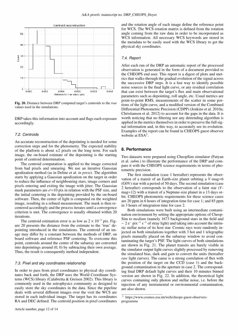
Fig. 20. Distance between DRP computed target’s centroids to the truevalues used in the simulations.

DRP takes this information into account and flags each exposureaccordingly.

7.2. Centroids

An accurate reconstruction of the depointing is needed for somecorrection steps and for the photometry. The expected stabilityof the platform is about ±2 pixels on the long term. For eachimage, the on-board estimate of the depointing is the startingpoint of centroid determination.

The centroid computation is applied to the image correctedfrom bad pixels and smearing. We use an iterative Gaussianapodization method (as in Deline et al. in press). The algorithmstarts by applying a Gaussian apodization on the target in orderto reduce the influence of neighbouring stars, image corners andpixels entering and exiting the image with jitter. The Gaussianmask parameters are σ=10 pix in relation with the PSF size, andthe initial centering is the depointing provided by the on-boardsoftware. Then, the center of light is computed on the weightedimage, resulting in a refined measurement. The mask is then re-centered accordingly and the process iterates until a convergencecriterion is met. The convergence is usually obtained within 20iterations.

The centroid estimation error is as low as 2 × 10−3 pix. Fig-ure 20 presents the distance from the estimate to the ‘true’ de-pointing introduced in the simulations. The centroid of an im-age may differ by a constant between the methods of DRP, onboard software and reference PSF centering. To overcome thispoint, centroids around the center of the subarray are convertedinto depointings around (0, 0) by subtracting their own average.Thus, the result is consequently method independent.

7.3. Pixel and sky coordinates relationship

In order to pass from pixel coordinates to physical sky coordi-nates back and forth, the DRP uses the World Coordinate Sys-tems (WCS) library (Calabretta & Greisen 2002). This library iscommonly used in the astrophysics community as designed toeasily store the sky coordinates in the data. Since the pipelinedeals with several different images over the visit the WCS arestored in each individual image. The target has its coordinatesRA and DEC defined. The centroid position in pixel coordinates

and the rotation angle of each image define the reference pointfor WCS. The WCS rotation matrix is defined from the rotationangle coming from the raw data in order to be incorporated asWCS information. All necessary WCS keywords are stored inthe metadata to be easily used with the WCS library to get thephysical sky coordinates.

7.4. Report

After each run of the DRP an automatic report of the processedobservation is generated in the form of a document provided tothe CHEOPS end user. This report is a digest of plots and met-rics that walks-through the gradual evolution of the signal acrossthe successive DRP steps. It is a fast way to identify possiblenoise sources in the final light curve, or any residual correlationthat can exist between the target’s flux and main observationalparameters such as depointing, roll angle, etc. Usual metrics arepoint-to-point RMS, measurements of the scatter in some por-tions of the light curve, and a modified version of the CombinedDifferential Photometric Precision (CDPP) (Jenkins et al. 2010a;Christiansen et al. 2012) to account for the gaps in the data. It isworth noticing that no filtering nor any detrending algorithm isapplied in the metrics themselves in order to preserve the full sig-nal information and, in this way, to accurately see its evolution.Examples of the report can be found in CHEOPS guest observerwebsite at ESA2.

8. Performance

Two datasets were prepared using CheopSim simulator (Futyanet al. subm.) to illustrate the performance of the DRP and com-pare it with the CHEOPS science requirements in terms of pho-tometric precision.

The first simulation (case 1 hereafter) represents the obser-vation of a transit of an Earth-size planet orbiting a V-mag=6(G0V) star with a period of 50 days. The second simulation (case2 hereafter) corresponds to the observation of a faint star (V-mag=12) with a transit of a Neptune-size planet in a 13 days or-bit. CHEOPS photometric requirements for these science casesare 20 ppm in 6 hours of integration time for case 1; and 85 ppmin 3 hours of integration time for case 2.

Both simulations were built using an intermediate contami-nation environment by setting the appropriate options of Cheop-Sim to medium (namely 1673 background stars in the field and∼ 2 e− pix−1 s−1 of stray light) and taking into account the intrin-sic stellar noise of its host star. Cosmic rays were randomly in-jected on both simulations together with 3 hot and 1 telegraphicpixels manually placed on the subarray window to avoid con-taminating the target’s PSF. The light curves of both simulationsare shown in Fig. 21. The planet transits are barely visible inthe simulator output light curves slightly processed by removingthe simulated bias, dark and gain to convert the units (hereafterraw light curves). The cause is a strong correlation of flux withthe position of the target on the CCD (case 1) and the back-ground contamination in the aperture in case 2. The correspond-ing final DRP default light curves and their 10 minutes binnedversion are shown in Fig. 22. In addition, the theoretical lightcurves containing only photon and stellar noise, i.e. before theinjection of any instrumental or environmental contamination,are also shown.

2 https://www.cosmos.esa.int/web/cheops-guest-observers-programme



Table 1. CDPP estimations from the final light curves of the case 1and 2 (see text for description). The first column shows the integrationtime used for the metrics, the second column shows the photometricrequirements for each case and the final columns shows the respectivenoise estimation of each analyzed light curve.

Science Int. Time Req. Modified CDPPCase (hours) (ppm) Theor. Default Optimal

1 6 20 5 6 52 3 85 62 117 83

2 w/o CR 3 85 62 69 67

The modified CDPP at different time scales is used to assesthe photometric precision of the light curves for each case. Itaccounts for the gaps in the light curves and is based on the meanof the unbiased variance estimates from a rolling window of aspecific time length. Then, the reported CDPP value correspondsto the square root of the mean of the variances normalized by themaximum number of points in the rolling windows. This metriccan be interpreted as the noise one would obtain by rebinningthe light curve at the selected time scale, time correlated or rednoise included. As explained before, no detrending nor filteringis applied within the metrics.

The obtained CDPP is shown at different time scales inFig. 23. For case 1, the DRP light curve reaches a precision be-low 6 ppm in 6 hours of integration time with a duty cycle of90% in the 24 hours of the visit.

The noise estimation for case 2 is 117 ppm in 3 hours of inte-gration for the same duty cycle. For its part, the optimal aperture(not shown in Fig. 23) delivers a dispersion of 83 ppm while thedispersion of the theoretical light curve is 62 ppm in the sameconditions. The case 2 light curve is evidently affected by unde-tected cosmic rays (Fig. 22). This effect is not surprising sincethe long exposure time (60 s) used in case 2 translates in a largernumber of CR per image for an equivalent integrated flux (seefor example Futyan et al. subm.). Furthermore, in this observa-tion no imagettes are available to help the cosmic rays detection.Confirming this effect, a control simulation with no cosmic raysinjected gives dispersion of only 70 ppm (resp. 67 ppm with theoptimal aperture) comparable to the theoretical case of 62 ppm.

Regarding the detection of the hot and telegraphic pixels, thepipeline was able to recover both hot pixels out from a dark cur-rent 3 to 5 times larger than the usual one and the inserted tele-graphic pixel was also correctly flagged. There were a few falsedetections, most of them close to the target, but they have noinfluence on the result since the DRP is not correcting but com-municating them for posteriori long term analysis.

9. Conclusions

The CHEOPS data reduction pipeline in its pre-launch versionhas been presented in this paper with a detailed description ofthe core processing stages of the calibration, correction and pho-tometry modules. The particularities of CHEOPS data and theirtreatments by the pipeline have also been discussed. In addition,two representative examples of scientific cases for CHEOPShave been used to evaluate the expected performance of thepipeline. For each case, the achieved photometric precision isgiven at different time scales. These examples show that the re-sults of the DRP are fully compliant with the scientific require-ments of the mission.

Even for challenging observations, such as for faint targets(e.g. case 2 in Sect. 8) the light curve derived by the DRP is notfar from ideal results. It was shown that for a V-mag=12 target,

Fig. 21. Light curves of raw data of case 1 (top) and case 2 (bottom).The raw data has been only corrected for bias, dark and gain for unitsadaptation.

Fig. 22. DRP light curves with the default aperture (gray) in case 1 (top)and 2 (bottom). Blue points are the 10 min binned version. Red pointsare the unbinned theoretical light curve arbitrarily shifted for better vi-sualization.

the 3-h dispersion of the light curve derived with the optimalmask is very close to the noise level of the theoretical photom-etry: 83 ppm vs 62 ppm, respectively. In fact, this could evenbe improved by performing clipping of photometric outliers orflux binning, for example. These treatments are left to the userssince best results are usually reached by a case by case detailedanalysis which strongly depends on the science goals of the ob-servations. As shown in Sect. 8, the deviations from theoreticalexpected performance of CHEOPS is not driven by instrumen-tal effects but by the influence of external agents such as smeartrails of background stars, cosmic rays and/or background con-tamination. The pipeline has proven that it is able to mitigatesuccessfully these effects on the final photometry even thoughimprovements, in particular, in cosmic ray detections are stillunder study and will be finally tested when the in-flight PSF isavailable.

DRP generates various output products the user will retrievefrom the archive: four light curves calculated with different aper-ture sizes, each with its contamination curve and associated un-certainties. The user will also get the report automatically gen-



Fig. 23. Noise estimations for the case 1 and 2 light curves. The plotsare the modified CDPP of the raw (black), default DRP (gray) and the-oretical light curves. The photometric requirement for each case is rep-resented by the blue dash at 6 and 3 hours for case 1 and 2, respectively(see text).

erated by the pipeline which intends to allow the user to followwhat treatment has been done on the data, the quality of the pro-cessing and of the final result. In addition to these final products,the user will have the possibility to get additional by-productsof the processing, such as, for example, bad pixel maps or thebackground light curve.

After the launch, the pipeline will be tuned and adapted toreal in-flight data: algorithms and modules will be improved allalong the mission lifetime with our increasing knowledge andunderstanding of the instrument to allow the best characteriza-tion of the transiting planets CHEOPS will observe.

The pipeline and its associated reference files are under ver-sioning control and therefore the data can be easily re-processedif it is required by CHEOPS project.

Acknowledgements. The DRP team thanks our referee, F. Claus, for his verycareful reading of the paper and his valuable comments and suggestions whichhelp us to improve the quality of the manuscript. We also thank D. Futyanfor his valuable support on Cheopsim. We gratefully acknowledge the SOCteam and the CHEOPS science team members who evaluated the pipeline re-sults, for their constant support in the realization of the CHEOPS pipeline andtheir helpful suggestions which allowed significant improvements of key reduc-tion steps. We thank K. Isaak for her careful reading and valuable feedbackon the manuscript. We thank also A. Cameron and D. Queloz for providingcomments that improved the paper. The team at LAM acknowledges CNESfunding for the development of the CHEOPS DRP, including grants 124378for O.D. and 837319 for S.H., and the support of the Direction Technique ofINSU with P.G. assignment. S.G.S also acknowledges support from FCT (FCT- Fundação para a Ciência e a Tecnologia) through Investigador FCT contractsnr.IF/00028/2014/CP1215/CT0002. O.D. is also supported by FCT contract DL57/2016/CP1364/CT0004. This work was supported by FCT/MCTES throughnational funds (PIDDAC) by the grant UID/FIS/04434/2019, by FCT funds(PTDC/FIS-AST/28953/2017) and by FEDER - Fundo Europeu de Desenvolvi-mento Regional through COMPETE2020 - Programa Operacional Competitivi-dade e Internacionalização (POCI-01-0145-FEDER-028953).

Software: The DRP is developed in Python 3 (PythonSoftware Foundation, https://www.python.org/), and makesuse of Astropy (Astropy Collaboration et al. 2013; Price-Whelan et al. 2018), Matplotlib (Hunter 2007), Numpy(https://www.numpy.org/), Scipy (Jones et al. 2001–) amongother Python open source libraries. Jupyter notebooks (Kluyveret al. 2016) were also used for the developing and testing of thecode.

ReferencesAstropy Collaboration, Robitaille, T. P., Tollerud, E. J., et al. 2013, A&A, 558,

A33

Baglin, A., Chaintreuil, S., Vandermarcq, O., & CoRot Team. 2016, II.1 TheCoRoT observations, 29

Benz, W., Ehrenreich, D., & Isaak, K. 2018, CHEOPS: CHaracterizing ExO-Planets Satellite, 84

Broeg, C., Benz, W., & Fortier, A. 2018, in 42nd COSPAR Scientific Assembly,Vol. 42, E4.1–5–18

Broeg, C., Benz, W., Thomas, N., & Cheops Team. 2014, Contributions of theAstronomical Observatory Skalnate Pleso, 43, 498

Calabretta, M. R. & Greisen, E. W. 2002, A&A, 395, 1077

Christiansen, J. L., Jenkins, J. M., Caldwell, D. A., et al. 2012, PASP, 124, 1279

Deru, A., Chaintreuil, S., Baudin, F., Ferrigno, A., & Baglin, A. 2015, in Euro-pean Physical Journal Web of Conferences, Vol. 101, 06022

Evans, D. W., Riello, M., De Angeli, F., et al. 2018, A&A, 616, A4

Fortier, A., Beck, T., Benz, W., et al. 2015, in Pathways Towards Habitable Plan-ets, 76

Hunter, J. D. 2007, Computing in Science & Engineering, 9, 90

Iglesias, F. A., Feller, A., & Nagaraju, K. 2015, Appl. Opt., 54, 5970

Jenkins, J. M., Caldwell, D. A., Chandrasekaran, H., et al. 2010a, ApJ, 713, L120

Jenkins, J. M., Caldwell, D. A., Chandrasekaran, H., et al. 2010b, ApJ, 713, L87

Jones, E., Oliphant, T., Peterson, P., et al. 2001–, SciPy: Open source scientifictools for Python, [Online, http://www.scipy.org/]

Kluyver, T., Ragan-Kelley, B., Pérez, F., et al. 2016, in Positioning and Powerin Academic Publishing: Players, Agents and Agendas, ed. F. Loizides &B. Schmidt, IOS Press, 87 – 90

Pinheiro da Silva, L., Rolland, G., Lapeyrere, V., & Auvergne, M. 2008, MN-RAS, 384, 1337

Powell, K., Chana, D., Fish, D., & Thompson, C. 1999, Appl. Opt., 38, 1343

Price-Whelan, A. M., Sipocz, B. M., Günther, H. M., et al. 2018, AJ, 156, 123

Rauer, H., Catala, C., Aerts, C., et al. 2014, Experimental Astronomy, 38, 249


expected performances of the characterising exoplanet

Documents