Expectations with Endogenous Information Acquisition:An Experimental Investigation∗

Andreas Fuster

Swiss National Bank

Ricardo Perez-Truglia

University of California, Los Angeles

Mirko Wiederholt

Sciences Po

Basit Zafar

Arizona State University

This Draft: December 2018Abstract

Information frictions play an important role in many theories of expectation formationand macroeconomic fluctuations. We use a survey experiment to generate direct evidenceon how people acquire and process information, in the context of national home price ex-pectations. Participants can buy different pieces of information that could be relevant forthe formation of their expectations about the future median national home price. We usean incentive-compatible mechanism to elicit their maximum willingness to pay. We also in-troduce exogenous variation in the value of information by randomly assigning individualsto rewards for the ex-post accuracy of their expectations. Consistent with rational inatten-tion, individuals are willing to pay more for information when they stand to gain more fromit. However, underscoring the importance of limits on information processing capacity, in-dividuals disagree on which signal they prefer to buy. Individuals with lower education andnumeracy are less likely to demand information that has ex-ante higher predictive power. Asa result of the disagreement, lowering the information acquisition cost does not decrease thecross-sectional dispersion of expectations. We show that a model with rational inattentionand heterogeneous prior beliefs about information sources can match almost all of our empir-ical results. Our findings also have implications for the design of information interventions.

JEL Classification: C81, C93, D80, D83, D84, E31, E58.Keywords: expectations, experiment, housing, information frictions, rational inattention.

∗Fuster: andreas.fuster@gmail.com. Perez-Truglia: ricardo.truglia@anderson.ucla.edu. Wiederholt:mirko.wiederholt@gmail.com. Zafar: basitak@gmail.com. We would like to thank Christopher Carroll, TheresaKuchler, Michael Weber and seminar attendants at the Arizona State University, ECB, Federal Reserve Board,Federal Reserve Bank of New York, Goethe University, EIEF Rome, the GEM/BPP Workshop, the CESifo VeniceSummer Institute and the AEA Annual Meetings for useful comments. Felipe Montano Campos provided superbresearch assistance. We thank the UCLA Ziman Center for Real Estate’s Rosalinde and Arthur Gilbert Programin Real Estate, Finance and Urban Economics for funding. Fuster and Zafar were employed at the Federal ReserveBank of New York while much of this paper was written. The views presented here are those of the authors anddo not necessarily reflect those of the Swiss National Bank, the Federal Reserve Bank of New York, or the FederalReserve System.

1 Introduction

Given the centrality of expectations in decision-making under uncertainty, consumer expectationshave been the focus of much research, particularly in macroeconomics. Studies have found con-siderable dispersion in consumers’ expectations (Mankiw, Reis, and Wolfers, 2003). The literaturehas theorized that this dispersion results from “rational inattention,”1 which may arise due to thecosts of acquiring information, as in the sticky information models of Mankiw and Reis (2002)and Reis (2006), or due to constraints on individuals’ information processing capacity, as in Sims(2003) and Woodford (2003). However, there is little direct empirical micro evidence that showshow individuals acquire and process information in the real world.2 In this paper, we present asurvey experiment to study the causes and consequences of information acquisition and processingdecisions.

We study information acquisition in the context of expectations about national home prices.Our interest in home prices stems from the fact that home price expectations play a prominentrole in many accounts of the housing boom that occurred during the mid-2000s in the UnitedStates (e.g., Shiller, 2005; Glaeser and Nathanson, 2015). These home price expectations havebeen measured with survey data, and these survey measures have been shown to be associatedwith real behavior such as buying or making investments in a home (Armona, Fuster, and Zafar,2017; Bailey et al., 2018). Given the prominence of housing in household portfolios, these decisionscan have substantial welfare consequences.

We design a survey experiment to test a series of predictions of the inattention models. Themain survey we use was conducted through the Federal Reserve Bank of New York in February2017, as part of a regular online survey on housing issues. The experimental design has four mainstages. In the first stage, respondents report their expectations about the national median homeprice for the end of the year (their “prior belief”). In the second stage, which occurs much laterin the survey, respondents are informed that their forecast will be re-elicited and incentivized: ifit falls within 1% of the realized price, the respondent is eligible for a monetary reward. Half ofthe subjects are randomly assigned to a reward that pays $100 with a probability of 10%, and theother half is assigned to a reward that pays $10 with a probability of 10%.

Before the belief re-elicitation, respondents are given the opportunity to choose among differentpieces of information that could be potentially useful for their forecasts: the average expert forecastof home price growth during 2017 (this forecast was +3.6% at the time of the survey), the nationalhome price change over the past one year (+6.8%), or the national home price change over thepast ten years (-0.9%, or -0.1% annually). Respondents also can choose no information at all.

1We use “rational inattention” in the broad sense of referring to all models where there is some trade-off betweenexpectations incorporating all available information optimally and some cost of doing so (as opposed to the narrowerentropy-based approach of Sims, 2003).

2In a recent survey article, Gabaix (2017) makes the case for more experimental evidence on the determinantsof attention, and the consequences of inattention.

2

These information pieces differ markedly in terms of their informativeness. For instance, onereasonable criterion, although certainly not the only one, is the information’s ex-ante predictivepower during the years leading up to the survey. Based on this criterion, the expert forecast isthe most informative (RMSE of 2.8), followed by the past one-year change (RMSE of 3.2), andthe ten-year change (RMSE of 7.9). This ranking of informativeness is consistent with findingsfrom the real estate literature. For instance, the fact that past one-year price changes performbetter than ten-year changes is consistent with the well-documented momentum in home pricesover short horizons (Case and Shiller, 1989; Guren, 2016; Armona et al., 2017).

In the third stage, we elicit the respondent’s maximum willingness to pay (WTP) for themost preferred information type. We use a multiple-price-list variation of the method of Becker,DeGroot, and Marschak (BDM): we ask individuals to choose either information or a paymentbetween $0.01 and $5 in eleven scenarios. One scenario is then randomly chosen, and the corre-sponding choice is implemented. Finally, the survey concludes with the re-elicitation of home priceexpectations (the “posterior belief”).

This experiment was designed to capture some important features of models of endogenous in-formation acquisition and processing. On the one hand, sticky information models (e.g., Mankiwand Reis, 2002; Reis, 2006) propose that information frictions arise due to costs of information ac-quisition. Agents update their information sets at a given point in time when the expected benefitexceeds a fixed cost of updating. Conditional on updating, agents have full-information rationalexpectations. On the other hand, noisy information models (e.g., Sims, 2003; Woodford, 2003;Mackowiak and Wiederholt, 2009) highlight the importance of limited information processing ca-pacity – in other words, even if information is freely available and agents continuously update theirinformation sets, individuals may not use all of it or may use it inefficiently. To explore these fea-tures, our experimental design creates exogenous variation in the cost of acquiring information andexogenous variation in the reward to holding an accurate posterior. Moreover, in the experiment,individuals can choose between different pieces of information with different levels of informative-ness. To explore the sticky information mechanism, we study how the information-acquisition costaffects posterior beliefs. To explore the noisy information mechanism, we investigate how the sizeof the reward and numeracy/financial literacy (our proxy for attention cost) affect the choice ofthe piece of information and the processing of the piece of information conditional on informationbeing displayed.

Our first result, with regards to preferences over pieces of information, indicates that individ-uals disagree on which piece of information to use: 45.5% chose the forecast of housing experts,28% chose the past one-year home price change, and 22% chose the past ten-year home pricechange. The remaining 4.5% reported to prefer no information at all. Thus, less than half of thesample chose the option that was most informative according to ex-ante predictive power. Someof this heterogeneity could be due to respondents using other criteria.3 However, sophisticated

3This finding could be partly driven by the fact that some respondents distrust experts (Silverman, Slemrod,

3

respondents, as measured by their education or numeracy, were substantially more likely to choosethe expert forecast than less sophisticated respondents. This finding suggests that at least part ofthe variation was due to cognitive limitations in identifying informative signals.

Our second result indicates that individuals demonstrate significant WTP for their favoriteinformation: the average individual was willing to forego $4.39. This WTP suggests that individ-uals expect to benefit from this information beyond the accuracy rewards provided in the survey.Interestingly, individuals are willing to pay a significant amount of money for information that ispublicly available for free. Furthermore, we find strong support for a basic prediction of modelsof endogenous information acquisition and processing: the average WTP is significantly higher inthe $100-reward condition than in the $10-reward condition ($4.80 and $3.99, respectively). Thisdifference is statistically significant (p-value<0.01) and economically meaningful. In addition, wefind that the amount of time spent choosing and processing information is weakly higher in thehigh-reward condition. However, we do not find that the ranking of pieces of information variessignificantly by reward size. This suggests that individuals would need some form of guidance onwhich information is most useful.

Our third result exploits the information-provision experiment to study how the informationacquired by the individuals affects their expectations. Our research design does not distinguishbetween rational expectations and some of its alternatives.4 Instead, our design measures whetherindividuals incorporate certain pieces of information into their forecasts. Consistent with a genuineinterest in information, individuals incorporate the information that they were willing to pay forinto their forecast: they form posterior beliefs by putting, on average, 38% weight on the signalbought and 62% on their prior belief. As evidence of genuine learning, we show that the informationprovided in the baseline survey had a persistent effect on a follow-up survey conducted four monthslater. The rate of learning was similar across all three pieces of information, which confirms thatthe disagreement about the ranking of pieces of information was meaningful. However, we findpatterns that at first sight run counter to the basic model of Bayesian updating. In particular,we find no evidence that individuals who had more uncertain prior beliefs put more weight on thepurchased information.

Our final result is about the effect of endogenous information acquisition on the cross-sectionaldispersion in beliefs. We measure the effect of the effective price of information (which was ran-domly assigned) on the dispersion of expectations. We find that a lower cost of informationacquisition does not cause lower cross-sectional dispersion in expectations. To understand the

and Uler, 2014; Cavallo, Cruces and Perez-Truglia, 2016; Cheng and Hsiaw, 2017). We provide direct evidenceabout this mechanism using an auxiliary survey.

4In recent years, several models of expectation formation have been put forward that deviate from rationalexpectations or Bayesian updating, such as experience-based learning (Malmendier and Nagel, 2016), natural ex-pectations (Fuster, Hebert, and Laibson, 2012), and diagnostic expectations (Bordalo, Gennaioli, and Shleifer,2017). This has also led to a literature, discussed below, that investigates the updating of expectations in styl-ized information experiments. These papers all provide evidence on how signals are incorporated in revisions ofexpectations, but abstract away from the process of acquiring the signals – the focus of this paper.

4

reason, we divide respondents into groups, based on their preferred information piece. On the onehand, exposure to information tends to reduce the dispersion in posterior beliefs within a group.For example, among individuals who preferred the expert forecast (a signal of 3.6%), exposure toit results in their posterior beliefs becoming more compressed around 3.6%. On the other hand,exposure to information increases the dispersion in beliefs across these three groups, because eachgroup acquires a different signal and the signals were far apart. These opposing effects are similarin magnitude, and thus end up canceling each other out.5 Additionally, we show that this resultis not an artifact of respondents being able to view only one piece of information – in an auxiliarysurvey with a similar set-up except that individuals are allowed to view multiple pieces of informa-tion simultaneously, we confirm that exposure to information does not cause lower cross-sectionaldispersion. Finally, contrary to the prediction of sticky information models, dispersion in beliefsremains high within each group of individuals who acquire the same information.

We next show that most of our experimental findings can be explained by a model of ratio-nal inattention with cross-sectional heterogeneity in the cost of the attention, and where agentshave heterogeneous beliefs about the precision of information sources. For example, with rationalinattention, the model can match the empirical result that time spent on processing informationis positively related to the reward size. The heterogeneity in perceived precision of informationsources can explain why our respondents choose different information sources. In addition, underthe assumption that the precision of prior beliefs is positively correlated with tastes for informa-tion (that is, respondents who enter the experiment with more precise beliefs intrinsically valueinformation more), we can reconcile the seemingly puzzling experimental finding that individualswith more precise (that is, less uncertain) beliefs put more weight on the displayed information.

This paper is related to various strands of literature. First and most importantly, it is relatedto a growing body of work on rational inattention models (Mankiw and Reis, 2002; Sims, 2003;Woodford, 2003; Reis, 2006). We contribute to this literature by providing direct empirical mi-cro evidence on how individuals acquire and process information in the real world. Our resultsare broadly consistent with these models. Specifically, the finding that cross-sectional dispersiondoes not decrease when the cost of information is lowered suggests that noisy information models(opposed to sticky information models) are a better characterization of the expectation formationprocess of consumers. In that sense, our conclusion is consistent with Coibion and Gorodnichenko(2012), who exploit the relationship of disagreement to shocks to distinguish between inatten-tion models. Their setup is quite different since it does not involve the endogenous process ofinformation acquisition, and uses observational data (opposed to experimental variation, as in ourcase).

5This finding has some parallels with the literature on media bias and political attitudes, according to whichdispersion in beliefs can be persistent because voters self-select into different information sources (Mullainathanand Shleifer, 2005). The underlying mechanisms, however, are different: in the political economy literature thedifferences in information choices arise due to self-serving biases, while in our context the differences in choicesseem to arise due to differences in preferences over information sources and/or cognitive limitations.

5

This paper is also related to a literature on the sources of dispersion in consumer expectations.For example, Figure 1 shows the distribution of housing expectations among consumers and ex-perts. Consistent with the evidence for other types of macroeconomic (Mankiw et al., 2003; Cavalloet al., 2017), this figure shows that housing expectations are substantially more dispersed amongconsumers than among experts. Our findings shed some light on the sources of this dispersion.Our evidence suggests that constraints in information processing play a big role in explaining thisdispersion: the dispersion in expectations arises because individuals differ in how much they arewilling to pay for information as well as what type of information they want to acquire. As aresult, even if the acquisition cost of information went down to zero, our findings imply that wewould still observe substantial dispersion in consumers’ expectations. This finding may explainwhy dispersion in expectations among consumers tends to be much larger than it is among expertseven though the estimated information acquisition costs are not larger for consumers (Coibion andGorodnichenko, 2012).

Our approach is related to a recent literature on information-provision experiments. Partic-ularly relevant for our purposes are papers that employ information experiments in surveys tounderstand expectation formation in the context of inflation (Armantier et al., 2017; Cavallo etal., 2017; Coibion, Gorodnichenko, and Kumar, 2015) or housing (Armona et al., 2017). The exper-iments in the context of inflation find that when individuals are provided with official statistics, thedispersion in expectations substantially decreases.6 The evidence from the information-provisionliterature provides suggestive evidence in favor of costly information acquisition models: once apiece of information is provided by the experimenter for free, the dispersion in expectations isreduced. However, information-provision experiments ignore a crucial aspect of the real world:individuals have to choose from multiple information sources, and where they look for informationcan be even more important than how frequently they look for information. Our findings indi-cate that, once respondents are allowed to choose information endogenously, reducing the cost ofinformation may fail to reduce dispersion in expectations.

Finally, our results have implications for the design of information interventions. A growingbody of research shows that, in a wide range of contexts, providing individuals with accurateinformation can have substantial effects on their beliefs and decisions (e.g., Duflo and Saez, 2003;Allcott, 2011; Cruces, Perez-Truglia, and Tetaz, 2013; Wiswall and Zafar, 2015). One of the policyimplications often drawn from this literature is that entities should make more information widelyavailable and easily accessible. Our evidence suggests that this strategy may not be sufficient,because individuals may not know which of the different pieces of information to focus on. Ourfindings imply that these interventions should either be targeted (providing consumers with limitedbut relevant information) or that they should guide consumers to help them interpret and weigh

6Endogenous information acquisition has been studied in other contexts, such as hiring decisions (Bartoš et al.,2016) and tax filing (Hoopes, Reck and Slemrod, 2015). Additionally, some laboratory experiments have been usedto study demand for information in stylized settings (e.g., Gabaix et al., 2006).

6

the various pieces of information.The rest of the paper proceeds as follows. Section 2 introduces the research design and survey

and outlines the testable hypotheses. Section 3 presents the results. The following Section 4describes the theoretical model and discusses how its predictions compare to the experimentalfindings. The last section concludes.

2 Survey Design

We designed a survey module to be embedded into the 2017 housing supplement of the FederalReserve Bank of New York’s Survey of Consumer Expectations (hereon, SCE Housing Survey).This survey has been fielded annually every February since 2014 and contains multiple blocksof questions, some of which distinguish between owners and renters.7 Among other things, thesurvey asks about perceptions of past local home price changes, expectations for future localhome price changes, and past and future intended housing-related behavior (e.g., buying a home,refinancing a mortgage). Respondents also provide information about their locations and manyother demographic variables.

The SCE Housing Survey is run under the Survey of Consumer Expectations, an internet-basedsurvey of a rotating panel of approximately 1,400 household heads from across the United States.The survey, as its name suggests, elicits expectations about a variety of economic variables, suchas inflation and labor market conditions. Respondents participate in the panel for up to twelvemonths, with a roughly equal number rotating in and out of the panel each month.8 Active panelmembers who participated in any SCE monthly survey in the prior eleven months were invited toparticipate in the housing module. Out of 1,489 household heads on the panel that were invited,1,161 participated, implying a response rate of 78%. Item non-response is extremely uncommonand rarely exceeds 1% for any question. The total survey time for the median respondent was 37minutes; we will later report time spent on specific questions analyzed here as a measure of effortspent on acquiring and processing information.

2.1 Research Design

Appendix D provides screenshots of the relevant module. The broad organization of the modulewas as follows:

7See Armona et al. (2017) and https://www.newyorkfed.org/microeconomics/sce/housing#main.8The survey is conducted over the internet by the Demand Institute, a non-profit organization jointly operated

by The Conference Board and Nielsen. The sampling frame for the SCE is based on that used for the ConferenceBoard’s Consumer Confidence Survey (CCS). Respondents to the CCS, itself based on a representative nationalsample drawn from mailing addresses, are invited to join the SCE internet panel. The response rate for first-timeinvitees hovers around 55%. Respondents receive $15 for completing each survey. See Armantier et al. (2016) foradditional information.

7

1. Stage 1- Prior Belief: This stage elicits individuals’ expectations of future national homeprice changes. Respondents were informed that, according to Zillow, the median price of ahome in the United States was $193,800 as of December 2016.9 The respondents were askedfor a point forecast: “What do you think the value of the typical home in the U.S. will beat the end of this year (in December 2017)?” To prevent typos in the responses, the surveyenvironment calculated and reported the implied percentage change after individuals enteredthe value. Individuals could confirm the number and proceed to the next screen or revisetheir guess. We refer to the response to this question as the respondent’s “prior belief.” Thesurvey also elicited the respondents’ probability distribution over outcomes around their ownpoint estimate: specifically, they were asked to assign probabilities to five intervals of futureyear-end home price changes: more than 10% below their point forecast; between 10% and1% below their forecast; within +/-1% of their forecast; between 1% and 10% above theirforecast; and more than 10% above their forecast.

2. Stage 2- Information Preferences: After answering a block of other housing-relatedquestions for roughly 15 minutes, respondents entered the second stage. They were notifiedthat the same questions about future national home prices that were asked earlier in thesurvey would be asked again, except this time their responses would be incentivized: “Thistime, we will reward the accuracy of your forecast: you will have a chance of receiving $[X].There is roughly a 10% chance that you will be eligible to receive this prize: we will select atrandom 60 out of about 600 people answering this question. Then, those respondents whoseforecast is within 1% of the actual value of a typical U.S. home at the end of this year willreceive $[X].” We randomly assigned half of the respondents to X=$100 (“High Reward”)and the other half to X=$10 (“Low Reward”).

Before providing their forecast, respondents were given an opportunity to see a potentiallyrelevant piece of information: “Before you report your forecast, you will have the opportunityto see only one of the following pieces of information that may help you with forecastingfuture year-ahead U.S. home prices. Please rank the following pieces of information on a 1to 4 scale, where 1 is “Most Preferred” and 4 is the “Least Preferred”:

• Change in the value of a typical home in the U.S. over the last one year (2016).

• Change in the value of a typical home in the U.S. over the last ten years (2007-2016).

• Forecasts of a panel of housing experts about the change in U.S. home prices over thiscoming year (2017).

• None of the above – I would not like to see any information.”

9They were then asked how the price changed over the prior one year (since December 2015) and the prior tenyears (since December 2006). They also were asked to rate their recall confidence on a 5-point scale.

8

Respondents were asked to drag and drop each of their selected rankings into a table withlabels from “1=Most Preferred” to “4=Least Preferred.”

3. Stage 3- Willingness-to-Pay for Information: This stage, which immediately followedthe second stage, elicited the respondents’ maximum willingness-to-pay (WTP) for theirhighest-ranked information type. Respondents who ranked “None of the above” as theirmost preferred information in Stage 2 skipped this stage. To assess WTP, we used the listprice method (e.g., Andersen et al., 2006) with eleven scenarios. In each scenario, respondentschose between seeing their preferred piece of information (i.e., the one they ranked highestin Stage 2) or receiving extra money in addition to their compensation for completing thesurvey. The amount of money offered in these scenarios was predetermined and varied in$0.50 increments, from $0.01 (in Scenario 1) to $5 (in Scenario 11). Respondents weretold that one of these eleven scenarios would be drawn at random and the decision in thatrandomly chosen scenario would be implemented.

4. Stage 4- Posterior Belief: In this stage, the respondent may have seen their highest-rankedinformation choice, depending on the randomly chosen scenario in Stage 3 and their choiceto see or not see the information in that scenario.10 Year-ahead home price expectations (thepoint estimate and the subjective belief distribution) that were elicited in Stage 1 were re-elicited from all respondents. We used the Zillow Home Value Index (ZHVI) as the source forprices of the typical (median) home in the U.S. over the last one or ten years.11 According tothe ZHVI, U.S. home prices decreased by 0.1% per year on average (or 0.9% in total) over theten years 2007-2016 and increased by 6.8% over the last one year (2016). The Zillow HomePrice Expectations Survey, a quarterly survey of about 100 economists, real estate experts,and market strategists, was the source for expert forecast.12 On average, experts forecastedan increase of 3.6% in home prices during 2017. Note that these information sources arepublicly available.

A paragraph providing the information followed a similar structure in all three cases. Theraw information was provided, followed by a naive projection of home prices in December2017 based on the annual growth rate implied by the information. For instance, respondentswho chose expert forecast were presented with “The average forecast of a distinguished panelof housing market experts who participate in the Zillow Home Price Expectations Survey isthat home values in the U.S. will increase by 3.6% over the next year. If home values wereto increase at a pace of 3.6% next year, that would mean that the value of a typical home

10In Stage 3, the scenarios 1-11 were picked with probabilities 0.15, 0.14, 0.13, 0.12, 0.11, 0.10, 0.09, 0.07, 0.05,0.03, and 0.01, respectively.

11For more information on the construction of the ZHVI, see http://www.zillow.com/research/ zhvi-methodology-6032/ (accessed on December 8, 2017). We used the ZHVI as of December 2016.

12For details, see https://pulsenomics.com/Home-Price-Expectations.php. We used the average forecast as ofthe fourth quarter of 2016.

9

would be 200,777 dollars in December 2017.” At the bottom of this same screen, expectationsabout year-end home prices were re-elicited. Respondents were reminded about their priorbelief. As in Stage 1, both the point estimate and subjective belief distribution were elicited.We refer to the point estimate from this stage as the “posterior belief.”

Afterwards, respondents were picked at random to be eligible for the incentive, as indicated inStage 2, and eligible respondents were informed at the end of the survey that they would be paidthe $10 (or $100) reward in case of a successful forecast (within 1% of the December 2017 ZHVI)in early 2018.13 At the end, respondents are also asked whether they used any external sources(such as Google or Zillow) when answering any question in the survey.

This summarizes the experimental setup. Four months after the initial survey, a short follow-up was fielded to active panelists in the June 2017 SCE monthly survey. As in Stages 1 and 4of the main experiment, respondents were asked to report their expectations about year-end U.S.median home prices. We kept the identical frame of reference in the follow-up survey: we providedindividuals with the median U.S. home price as of December 2016 and asked them to forecast thevalue in December 2017. Both the point estimate and subjective density were re-elicited. Of the1,162 respondents who took the SCE Housing Survey, 762 were still in the panel in June and henceeligible to take the follow-up survey. Of those, 573 did so, implying a response rate of 75.2%.

An additional module was fielded in the 2018 SCE Housing Survey. Since the main purpose ofthe module is some robustness checks and because that sample has no overlap with the sample inthe original study, we defer the details to Appendix B.

2.2 Discussion of the Experimental Design

Our design tries to mimic real-world information acquisition and processing, albeit in a stylizedsetting. Before turning to the empirical analysis, it is useful to discuss the features of the ex-perimental design and to outline the main hypotheses. Unless otherwise stated, the null is thatexpectations are formed according to a combination of a sticky information model, as in Reis(2006), and a rational inattention model, as in Sims (2003). The model is presented formally inSection 4.

A key feature of our setup is that respondents are presented with three possible pieces ofinformation, which they are asked to rank in terms of their preference, including a no-informationoption. We make it clear to respondents that they can see their top-ranked choice. Ideally, we wantto test whether individuals have some reasonable idea or consensus about the usefulness of theinformation. However, no single criterion can measure informativeness. One reasonable metric ofinformation usefulness is how well it has historically predicted past year-ahead home price changesin the United States.

13Payments to those who qualified and met the reward criterion were made in March 2018. 14 respondentsreceived a payout (half of them $100, the others $10).

10

Let HPAt denote the actual home price change during year t. Let HPAFt be the mean forecastof experts about home price changes for year t, HPAt−1 the annualized home price change overthe past 1 year, and HPAt−10 the annualized home price change over the past 10 years. For eachpiece of information It ∈ HPAFt , HPAt−1, HPAt−10, we define its informativeness as the rootmean squared error (RMSE) of a model HPAt = It. Thus, for the empirical analysis, we test aweaker version of the ideal hypothesis that is based on this specific metric of informativeness:

Hypothesis 1 (Preference for Informative Signals): The demand for an infor-mation source increases with its ex-ante predictive power.

To calculate the RMSE of each piece of information, we use the Zillow Home Value Index asthe outcome (that is, as our estimate of HPAt), because it is the same outcome that we areasking the subjects to forecast in our survey, and regress it onto each of the potential sources ofinformation. Using this data, the RMSE for experts’ forecast is 2.8, the RMSE for past one-yearchanges is 3.2, and the RMSE for past ten-year changes is 7.9 when using the longest availableseries (the experts’ forecast is available since 2010, and the ZHVI since 1996). Based on theseresults, the expert forecast has been the most informative in predicting year-ahead home pricechanges, followed by past one-year change, and then the ten-year change. This ranking remainsthe same when we use only data since 2010 for all three series (in this case, the one-year RMSEis 3.3, and the ten-year RMSE is 5.2). Using a longer home price index series from CoreLogic(starting in 1976), the ranking also remains consistent.14

This criterion for ranking the informativeness of the signals is broadly consistent with basicinsights from the real estate literature. First, the fact that the forecasts are ranked highest isconsistent with the view that forecasters use all available information in past home price changesoptimally when providing a forecast.15 Additionally, this criterion is consistent with the modelof Carroll (2003), in which consumers periodically update their expectations based on reportsof expert forecasts, which are assumed to be rational. Second, the higher ranking of past one-year home price change relative to past ten-year change is consistent with the well-documentedmomentum in home prices over short horizons (Case and Shiller, 1989; Guren, 2016; Armona etal., 2017). For instance, for the nominal CoreLogic national home price index from 1976–2017,the AR(1) coefficient of annual growth is 0.73 and highly statistically significant, with an R2 of0.57. This serial correlation is only slightly weaker if we calculate price growth in real terms (thecoefficient falls to 0.66 but remains highly significant).16 In contrast, regressing one-year growth

14Using the CoreLogic series, the RMSE is 4.6 for the average expert forecast (6 observations), 5.0 for the pastone-year change (39 observations), and 7.8 for the past ten-year change (30 observations).

15This should be true at least for the consenus forecast, even though individual forecasters may have incentivesto deviate for strategic reasons (e.g. Laster et al., 1999).

16It is also robust to using alternative home price indices, such as Case-Shiller. Further, momentum is similarlystrong at a more local level: Armona et al. (2017) find that in a regression of one-year home price changes onlagged one-year home price changes at the zip code level, the average estimate (across the zip codes in the U.S.) is0.53 (statistically significant with p < 0.01).

11

on growth over the previous ten years yields a small and insignificant negative coefficient.Although reasonable, our criterion is not the only one that can determine the usefulness of

information. For example, according to the ZHVI, U.S. home prices increased by 6.5% during2017. Thus, based on ex-post accuracy, using the past one-year change would have led to the mostaccurate expectation. By this same ex-post metric, however, it is hard to rationalize picking homeprice change over the past ten years over either of the other two pieces of information.

Turning to our next hypothesis, rational inattention predicts that, in the absence of an incentive(such as the lack of a direct stake in the housing market), individuals in the real world may investfewer resources in acquiring housing-relevant information and having more informed home priceexpectations.17 The randomization of the accuracy incentive in Stage 2 provides a direct testof this hypothesis: that is, whether higher stakes causes the respondents to be willing to paymore for information or to spend more time processing it. Moreover, rational inattention modelswith constraints on information processing capacity (Sims, 2003; Woodford, 2003; Mackowiak andWiederholt, 2009) predict that, when the stakes are high, respondents think carefully about theusefulness of potential information and hence rank information differently than their counterparts(in particular, they rank “None of the Above” lower). This leads to our second hypothesis:

Hypothesis 2 (Attention and Stakes): When the accuracy incentive is higher,individuals are more willing to pay for information and spend more time processing it;also, the higher accuracy incentive should make the individuals more likely to choosethe more informative sources.

Another feature of the design is that in Stage 4, some respondents get to see one of the pieces ofinformation. Whether a respondent sees their top-ranked information depends on the WTP andthe randomly picked scenario from Stage 3. This randomization generates random variation in theprovision of information, because for two individuals with identical WTPs in Stage 3, whether theinformation is shown in Stage 4 is determined at random. We exploit this aspect of the designto investigate whether respondents incorporate the signal into their posterior beliefs, as would beexpected if individuals were willing to pay for the information. Rational updating also implies thatindividuals who have uncertain prior beliefs put more weight on the information they receive.18

This leads to our third hypothesis:

Hypothesis 3 (Rational Updating): If individuals are willing to pay for a signal,they should incorporate that signal into their expectation formation once they get access

17This would follow from most sticky information models. For example, in the sticky updating model of Reis(2006), agents are modeled as maximizing utility subject to constraints, which also include costly information.Increasing the payoff for more informed expectations would lead more agents to incur the cost of acquiring housing-relevant information.

18Under Bayesian updating, the weight put on the signal is positively related to the uncertainty in the priorbelief, and inversely related to the (perceived or actual) noise in the signal. As long as the perceived noise in thesignal is independent of one’s uncertainty in the prior belief, Bayesian updating predicts that individuals with moreuncertain priors put more weight on the signal.

12

to it. The weight on the signal should be higher for those with higher prior uncertainty.

The last hypothesis is framed such that the null is the pure sticky information model (Reis, 2006).In this model, cross-sectional dispersion in beliefs arises only because some individuals update theirinformation sets to perfect information, while other individuals do not update their informationsets. If all individuals updated at a given point in time, there would be no cross-sectional dispersionin beliefs. When only some individuals update at a given point in time, there is no cross-sectionaldispersion in beliefs among those who update. This leads to our final hypothesis:

Hypothesis 4 (Information Acquisition and Dispersion of Expectations):Cross-sectional dispersion in beliefs arises mainly because some individuals acquire in-formation, while other individuals do not acquire information.

2.3 Sample Characteristics

Of the 1,162 valid responses, we trimmed the sample by dropping 43 respondents: those with priorbeliefs below the 2.5th percentile (an annual growth rate of -7.1%) or above the 97.5th percentile(an annual growth rate of 16.1%). These extreme beliefs may be the product of typos or lack ofattention. As the prior belief was reported before the treatments, dropping these extreme priorbeliefs should not contaminate the experimental analysis. For the posterior beliefs, these typos mayalso show up, but dropping individuals based on post-treatment outcomes could contaminate theexperimental analysis. Instead, we winsorize the post-treatment outcomes using the same extremevalues presented above (-7.1% and 16.1%).19 In any case, we use graphical analysis wheneverpossible to certify that the results are not driven by outliers.

Column (1) of Table 1 shows characteristics of the sample for the main survey. Most dimen-sions in the sample align well with average demographic characteristics of the United States. Forinstance, the average age of our respondents is 50.8 years, and 47.6% are females, which is similarto the corresponding 45.5 years and 48.0% among U.S. household heads in the 2016 AmericanCommunity Survey. Also, 74.8% of respondents in our sample are homeowners, compared to anational homeownership rate in the first quarter of 2017 of 63.6%, according to the AmericanCommunity Survey. Our sample, however, has significantly higher education and income: 55.2%of our respondents have at least a bachelor’s degree, compared to only 37% of U.S. householdheads. Likewise, the median household income of respondents in the sample is $67,500, which issubstantially higher than the U.S. 2016 median of $57,600. This may be partly due to differentinternet access and computer literacy across income and education groups in the U.S. population.Respondents expect national home prices to increase by 2.2%, on average, over the next year.

Columns (2) and (3) of the table show average characteristics for the subsamples assigned tothe low- and high-reward treatments, respectively; in turn, columns (5) and (6) show the char-

19For the beliefs from the follow-up survey, we winsorize the values in the same way. Results are robust underalternative thresholds.

13

acteristics for the subsamples assigned to the low- and high-price treatments. Columns (4) and(7) present p-values for the test of the null hypothesis that the characteristics are balanced acrosstreatment groups. The differences in pre-treatment characteristics are always small, and statis-tically insignificant in 19 out of the 20 tests. This is not surprising, because random assignmentshould preserve balance between the two groups. Additionally, the last row of Table 1 reports theresponse rate to the follow-up survey. The evidence rules out selective attrition: the response ratedoes not differ by reward or price treatments.

Table 2 provides additional information on how the follow-up sample compares with the initialsample. Column (1) show the average characteristics for the whole sample. Columns (2)–(4) breakdown the average observables by eligibility for the follow-up sample: the evidence shows that thesubsample that was eligible to be invited to the follow-up survey was similar to the ineligiblegroup of respondents who were phased out of the panel, with the differences being statisticallyand economically insignifciant. The final three columns of the table also are reassuring, as we seeno evidence that, conditional on being invited to the follow-up, the individuals who responded tothis survey are significantly different from the ones who did not.

3 Empirical Analysis

3.1 Hypothesis 1: Preference for Informative Signals

To understand how respondents acquire information, it is useful to describe the distribution ofexpectations prior to the information acquisition. Figure 2.a shows a histogram of the pointestimates provided by respondents. In terms of the implied annual growth rates, the mean (median)value is 2.2% (1.7%), with substantial dispersion across respondents: the cross-sectional standarddeviation of prior beliefs is 3.1%. To assess if individuals felt confident about their expectations,Figure 2.b shows the probability distribution of beliefs around the individual’s own point estimate,averaged over all individuals. On average, individuals thought there was a 51% chance that thetrue price would fall within 1% of their guesses. Moreover, there was high dispersion in the degreeof certainty. For example, 13% of the sample thought that there was a 90% chance or higher ofyear-end home prices being within 1% of their guess, and 16% of the sample thought that therewas a 20% chance or lower.20

What happens when individuals with uncertain beliefs are offered the chance to acquire in-formation? The median respondent spent 2.17 minutes choosing between the information sources(and reading the associated instructions), with 10th percentile at 1.23 minutes and 90th percentileat 4.85 minutes. Figure 3.a shows the ranking distribution for the different information types

20Ex post, only 3.5% of respondents had a prior forecast within 1% of the realized ZHVI price as of December2017, which was $206,300 (according to Zillow in January 2018), corresponding to realized growth over 2017 of6.5%. For the posterior forecast, this fraction increased to 11.5%.

14

over the whole population. Individuals disagreed on which of the three pieces of information theywould want to see: 45.5% chose forecasts of housing experts, 28.1% chose the last-one-year homeprice change, 22.1% chose the last-ten-year home price change, and the remaining 4.3% preferredno information. The past predictive power criterion indicated that expert forecast was most in-formative, followed by the last-one-year home price change and then the last-ten-year home pricechange. Thus, the popularity of the choice is increasing with its informativeness. However, thiscorrelation is far from perfect: less than half of the sample chose the most informative choice (i.e.,expert forecast).

This heterogeneity in the ranking of information could be driven by consumers’ lack of knowl-edge about the relative informativeness of the signals or by respondents using different criteria todetermine the informativeness of the signals. Systematic differences in ranking by education ornumeracy of respondents, which are reasonable proxies for ability to filter signals, would suggestevidence of the former.21 Figure 3.c and 3.d thus break down the information choices by respon-dents’ numeracy and education, respectively, and show that individuals with more education orwith higher numeracy were substantially more likely to choose the “best” information: collegegraduates chose the expert forecast 50% of the time, compared with non-graduates who chose it40% of the time (p-value<0.01).22

Table 3 further explores the heterogeneity and reports univariate relationships between thechoice of information and various individual- and location- specific characteristics.23 The dependentvariables in columns (1)–(3) correspond to dummy variables indicating the highest ranked pieceof information.24 Besides numeracy and education of respondents, only a handful of variables aresignificant, suggesting that observable characteristics (at the individual or location level) cannotexplain most of the heterogeneity in how individuals rank information. Homeowners are more likelyto choose the past-one-year information and less likely to choose the expert forecast, perhapsbecause they are curious to learn about how their housing wealth has evolved. Higher incomerespondents and white respondents are more likely to choose the expert forecast, although thesecoefficients are only marginally significant.

One might expect respondents who have high confidence in their perceptions of past homeprice changes to be more likely to choose the expert forecast (since they think they know the pastrealized growth already); however, if anything we see the opposite. Likewise, one might expectrespondents residing in states with volatile housing prices (as measured by the standard deviationin monthly home prices over the past 24 months) to be less likely to choose past home pricechanges. We do not find evidence of that.

21Numeracy is evaluated based on 5 questions taken from Lipkus et al. (2001) and Lusardi (2009). The rankcorrelation between education and numeracy in our sample is +0.31.

22Similarly, Burke and Manz (2014) find that respondents with higher levels of economic literacy choose morerelevant information when forming inflation forecasts.

23The results are similar using multivariate regressions, as reported in Appendix Table A.1.24The results are also robust if instead of a linear probability model we use a multinomial logit model.

15

In column (4), we study as an alternative outcome whether a respondent ranked the one-year realized growth higher than the 10-year realized growth (as would be optimal based on pastpredictive performance); we see little relation with observables, except that younger respondentsare more likely to prefer the longer-term data. College-educated and higher-numeracy respondentsare about 3 percentage points more likely to prefer one-year information, though neither estimateis very precise.

The supplementary survey that was conducted in 2018 provides some additional insights, whichare discussed in detail in Appendix B. First, we validate the finding that subjects disagree in termsof the information that they acquire, and that those disagreements are correlated with educationand numeracy. Second, the supplementary survey included a couple of additional questions to ex-plore the role of trust in experts as a driving factor for preferences over information sources. Overalllevels of trust in the credibility of experts and their ability to forecast accurately is moderate, andwe do find that less-educated respondents exhibit lower levels of trust in experts. However, whilea relevant explanation, distrust of experts is not the main factor driving the information choicesof our respondents: for instance, we find that these differences in trust can explain less than aquarter of the education gap in preferring experts.

We can summarize our first result as follows:

Result 1 : The information with the highest ex-ante predictive power, expert forecast,is the modal choice. The information with the second highest ex-ante predictive poweris the second most frequent choice. Considerable disagreement exists across householdson the ranking of information. The ranking is systematically related to measures ofrespondent ability, which suggests that cognitive limitations in deciphering informativesignals partially drives the heterogeneity.

3.2 Hypothesis 2: Attention and Stakes

Before we can test if higher stakes change the willingness to pay for information, it is usefulto understand the distribution of WTP for the whole sample. Using responses to the elevenscenarios, we identify the range of an individual’s WTP. For example, if an individual choseinformation instead of any amount up to $3 and then chose the money from $3.50 on, it meansthat the individual’s WTP must be in the range $3 to $3.5. Around 5% of respondents providedinconsistent responses; for example, they chose information instead of $3 but then chose $2.5instead of information. This inconsistency is within the range of other studies using this listmethod for elicitation of WTP for information. For instance, the share of inconsistent respondentswas about 2% in Allcott and Kessler (2015) and 15% in Cullen and Perez-Truglia (2017).

Figure 4.a shows the histogram of WTP based on this approach. We find that individualshave significant WTP for their favorite information, with a median maximum WTP between $4.5

16

and $5.25 This is fairly high WTP, given that the information we provide is publicly and readilyavailable using a search tool like Google. This finding indicates that most individuals are eitherunaware of the availability of this information or they expect a high search cost. Also, the medianWTP ($4.5-$5) is high, compared to the expected reward for perfect accuracy ($1 for half of thesample and $10 for the other half). This evidence suggests that individuals value the informationbeyond the context of the survey. They may want to use this information for real-world housingdecisions. In this context, having incorrect expectations about house prices can translate intothousands of dollars in losses, relative to which the experimental incentive pales in comparison.26

We next test Hypothesis 2, i.e., whether WTP, time spent choosing and processing information,and ranking of information systematically varies with reward size. Figure 4.b conducts a non-parametric test of this hypothesis by comparing the distribution of WTP between the two rewardgroups. This figure suggests that, consistent with the rational inattention hypothesis, individualsin the higher-reward treatment are willing to pay more. The Mann-Whitney-Wilcoxon (henceforthMWW) test indicates that this difference is statistically significant (p-value<0.01).

To better understand the economic magnitude of this difference, column (1) of Table 4 presentsthe rational inattention test in regression form. The constant reported in column (1) can beinterpreted as the mean WTP for the low-reward condition ($10 with 10% probability). Thisaverage valuation is estimated to be $3.99 (95% CI from 3.68 to 4.31). The coefficient on HighReward indicates that, relative to the $10 reward, individuals assigned to the $100 reward arewilling to pay an additional $0.80 for their favorite information (or 20% more). Note that theexpected reward goes from $1 to $10, because the reward is given only with 10% probability. The$0.80 difference in WTP then implies that for each additional dollar of expected reward, the WTPfor information goes up by 8.9 cents.

Another way to interpret the result is as follows:

WTPi = UInfo + 0.1 ·Rewardi · [Pi (Accurate|Info)− Pi (Accurate|NoInfo)] + εi. (1)

The first term, UInfo, represents the expected real-world benefit from having the informa-tion (e.g., because one expects to make better choices when deciding whether to buy a house).

25An alternative estimate is given by means of an interval regression model. This is a maximum likelihood modelthat assumes that the latent WTP is normally distributed. The constant in this model is estimated to be $4.39(95% CI from 4.16 to 4.63). This coefficient can be interpreted as the mean WTP under the implicit assumptionthat WTP can take negative values; if we instead assume that the WTP must be non-negative, then the meanwould be even higher.

26Additionally, we can compare the median WTP in our study ($4.5-$5) with the results from a few otherpapers that elicit WTP for information using similar methods. Those studies find lower valuations: $0.40 fortravel information (Khattak, Yim, and Prokopy, 2003), $0.80 for food certification information (Angulo, Gil, andTamburo, 2005), and $3 for home energy reports (Allcott and Kessler, 2015). Hoffman (2016), in a field experimentabout guessing the price and quality of actual websites, finds that business experts tend to underpay (overpay) forinformation when signals are informative (uninformative).

17

The second term reflects the benefits of information from the survey reward, under the sim-plifying assumption that the respondent is risk-neutral for small amounts. We can infer thevalue of Pi (Accurate|Info)−Pi (Accurate|NoInfo) from a regression of WTPi on 0.1 ·Rewardi.Indeed, we do not even need to run a new regression. We can recover that parameter fromthe coefficients on column (1) of Table 4.27 This estimator suggests that Pi (Accurate|Info) −Pi (Accurate|NoInfo) = 0.089. In other words, by acquiring the information, the average indi-vidual expects that the probability of being accurate (i.e., being within 1% of the realization) willincrease by 8.9 percentage points, or 17% of the baseline probability.28

It is worth asking whether the level of attention varies systematically with respondents’ abilities,as would be predicted under models of information rigidities due to cognitive limitations. Columns(2) and (3) of Table 4 investigate whether higher numeracy and higher education individuals aremore rationally attentive (i.e., more reactive to the higher reward). In column (2), the High-Rewarddummy is interacted with a standardized measure of numeracy. In column (3), the High-Rewarddummy is interacted with a dummy for college graduate. In column (2), the effect of high rewardis more than 50% larger (and statistically significant at the 10% level) for individuals with a one-standard-deviation higher numeracy. In column (3), the effect of high reward is 70% larger forcollege graduates relative to non-graduates, although the difference is imprecisely estimated andthus statistically insignificant.29 We already showed that highly educated and highly numeraterespondents are more likely to choose the expert forecast. So, not only are respondents with loweducation and numeracy less likely to rank information optimally, they also are less responsive tohigher rewards.

Given that individuals pay more for information when the stakes are high, the next questionis whether individuals choose information types differently when the stakes are high. Figure 3.bbreaks down the information choice by reward type. The choices are almost identical across bothgroups; the p-value of the difference is 0.89. Column (4) of Table 4 presents this same test inregression form. It corresponds to a linear probability model where the dependent variable iswhether the individual chooses the expert forecast (i.e., the “best” information type according topast predictive power). Column (4) implies that individuals are not more likely to choose expertforecast under the high reward. Additionally, Columns (5) and (6) of Table 4 show that the effectof the large reward on choosing the expert forecast does not differ by numeracy or education.

We can use the time spent making choices as an alternative measure of attention effort. Columns(7) through (9) use the time spent choosing between the information sources as the dependent vari-

27The coefficient on the High Reward dummy indicates that increasing 0.1 ·Rewardi by 9 (i.e., 0.1 ·100−0.1 ·10)increases the WTP by $0.80. Thus, increasing 0.1 ·Rewardi by 1 would increase the WTP by 0.089 (= 0.80

9 ).28The average individual responded that there was a 51.3% chance that their guess is within 1% of the true price.

We use this as an estimate of the average Pi (Accurate|NoInfo). Thus, the 8.9 percentage point effect translatesinto a 17% (=8.9/51.3) effect.

29Note the estimate for the High Reward dummy is no longer significant. On the other hand, the impact of theHigh Reward for college-educated respondents, which is the sum of the two estimates is a precisely estimated $0.98.Thus, the impact of the higher rewards on the WTP is primarily driven by college-educated respondents.

18

able.30 The results from column (7) indicate that, consistent with rational inattention, individualsassigned to the higher reward spent an additional 0.18 minutes choosing between informationsources (from a baseline of 2.65 minutes in the lower-reward condition), though the differenceis not quite statistically significant at conventional levels. Columns (8) and (9) show that morenumerate and more educated respondents take less time to respond, but are not differentiallysensitive to the higher reward.

Columns (10) through (12) use the time spent on the screen used to report the posterior beliefs.Due to the design of the survey, this variable includes the time spent looking at the information. Asa result, in these regressions we control for a dummy indicating whether the individual was providedwith information. The median time spent on reporting the posterior belief is 1.76 minutes for thelower-reward group. The results from column (10) suggest that the higher reward condition hada marginally significant positive effect on the time spent on this task (an additional 0.21 minutes,p<0.1). Again, we see no differential sensitivity to the rewards by education or numeracy.

This leads to our second result:

Result 2 : Consistent with rational inattention, the WTP for information is higherwhen the incentive is higher. Time spent choosing and processing information is alsoweakly higher when the incentive is higher. However, the ranking of information sourcesdoes not systematically differ by reward size.

Figure 4.a shows considerable heterogeneity in WTP. We next investigate the drivers of this het-erogeneity. Column (5) of Table 3 uses the interval regression model to estimate the effect of aset of factors on WTP, with the impact of each factor investigated one at a time. We see thathigher income respondents, older respondents, and homeowners have economically and statisticallysignificantly higher WTP for information. For instance, respondents with incomes above $60,000are willing to pay about 50 cents more than those with lower incomes. Gender, education, andnumeracy are not systematically related to WTP.

The expected effect of past search efforts on WTP is ambiguous. On the one hand, individualswho looked for information in the past may be willing to pay less for the information, because theyhave good information already. On the other hand, individuals who acquired more information inthe past may have the highest revealed demand for information and thus could be more willing tobuy additional information. Our evidence suggests that the second channel dominates: individ-uals who looked for housing-related information in the past were willing to pay an additional 57cents, relative to those who did not. Likewise, we can study how the uncertainty in prior beliefcorrelates with WTP. To measure uncertainty at the individual level, we use the responses to theprobability bins. We fit these binned responses to a normal distribution for each individual anduse the estimated standard deviation of the fitted distribution as a measure of individual-level

30We winsorize this time at 10 minutes, which is about the 98th percentile.

19

uncertainty, with higher values denoting higher uncertainty.31 When looking at the relationshipbetween uncertainty of prior beliefs and WTP, we again find evidence for the selection channel:individuals with a one-standard deviation higher uncertainty in their prior beliefs were, on average,willing to pay $0.32 less.32 Similarly, individuals who are more confident in their perceptions ofpast home price growth are willing to pay more for information.

The expected effect of local volatility in home prices on WTP also is ambiguous. On theone hand, updating more often is valuable for such respondents, and hence they should valueinformation more. On the other hand, past changes in home prices are less informative. Wehave seen that respondents in these areas do not choose expert forecast more often. Here, we seethat these respondents in fact value information more: increasing the home price volatility by 1standard deviation increases the WTP by 25 cents.

Finally, we know that experts’ forecasts historically have predicted home price changes moreaccurately than the other two information pieces. Under this metric, individuals then should bewilling to pay more for expert forecasts. However, if individuals select a given information sourcebecause they erroneously believe it to be the most accurate/predictive one, then the WTP shouldnot differ by information source. In an interval regression similar to the ones above, average WTP ishighest for the 10-year information, followed by the expert forecast and the 1-year information; thedifference between 10-year and 1-year information is significant at p<0.05 (while the coefficienton the expert forecast is not significantly different from either of the others). That is, there isno evidence that individuals pay more for information that has higher ex-ante predictive power.Panels c and d of Figure 4 break down the WTP by information type, showing how WTP forthe expert forecast compares with that for past-one-year and past-ten-year home price changes,respectively. The panels also report results from an MWW test of the null that the distributionsare identical, which is not rejected at conventional levels of significance.

3.3 Hypothesis 3: Rational Updating

Recall that our design generates random variation in whether a respondent saw information. Fortwo individuals with identical WTP (and conditional on top-ranked information), whether in-formation was shown to them was determined by chance. We use this random variation in theinformation provision to estimate the rate at which individuals use the signal to update their fore-cast. Furthermore, we calculate this learning rate for different sub-populations, particularly forsub-groups choosing different pieces of information.

31For instance, consider an individual with a 2% house price growth point forecast who has an uncertainty of 1percentage point. It means that the individual’s 95% confidence interval for house price growth is [0.04%, 3.96%](= [2− (1 ∗ 1.96), 2 + (1 ∗ 1.96)]).

32Note that the correlation of prior uncertainty with education/numeracy as well as with looking up housing-related information in the past is negative. This further suggests that the selection channel – of people genuinelyinterested in information having more precise priors and willing to pay more for information – being the dominatingfactor.

20

We use a simple learning model that naturally separates learning from the signal shown fromother sources of signal-reversion.33 Let bprior denote the mean of the prior belief, bsignal the signal,and bposterior the mean of the corresponding posterior belief. When priors and signals are normallydistributed, Bayesian learning implies that the mean of the posterior belief should be a weightedaverage between the signal and the mean of the prior belief:

bposterior = α · bsignal + (1− α) · bprior. (2)

The degree of learning can be summarized by the weight parameter α. In a Bayesian framework,the weight is proportional to the uncertainty (i.e., the variance) of the prior and inversely relatedto the uncertainty and noise in the signal. This parameter can take a value from 0 (individualsignore the signal) to 1 (individuals fully adjust to the signal). Re-arranging this expression, we getthe following:

bposterior − bprior = α ·(bsignal − bprior

). (3)

That is, the slope between the perception gaps (bsignalk −bpriork ) and revisions (bposteriork −bpriork ) canbe used to estimate the learning rate.34 However, it is possible that individuals will revise theirbeliefs towards the signal even if they are not provided with the signal. For instance, considersomeone who makes a typo when entering her prior belief and reports an estimate that differssignificantly from the signals. If that person does not commit the typo again when reporting theposterior belief, it will look like she is reverting to the signal despite not being shown information.Also, it is possible that individuals think harder the second time they are asked about their homeprice expectation, especially since the posterior belief is incentivized but the prior belief is not.Additionally, it is plausible that some individuals searched for more housing-related informationonline during the survey. At the end of the survey, we asked respondents whether they hadsearched for information online during the survey, explaining that doing so was permitted, and14.1% reported doing so. Interestingly, the search rate did not differ between respondents who sawinformation (14.3%) and those who did not (13.6%). Also, the simple act of taking a survey abouthousing may make respondents think more carefully about their responses and may lead them torevise their expectations even if they are not provided with any new information (see Zwane et al.,

33Similar learning models are used in Cavallo et al. (2017).34There is an alternative specification for this learning model. Consider the case when the information chosen

is the past 10 year home price change. bsignal is the actual past 10 year change, and ˆbsignali is i’s prior belief about

the past 10 year home price change, that was also elicited in the first stage of the survey. bsignal − ˆbsignalk is then

the difference between the actual change and the perceived change. The revision in expectations can be regressedonto this metric (this kind of learning model has been used in Amantier et al., 2016, and Armona et al., 2017). Wedo not use this alternative model for two reasons. First, this alternative model cannot be estimated for one of thedata sources, because we did not elicit the prior belief about the signal of professional forecasters. Second, whenconsidered simultaneously in the regression analysis, our baseline model fits the data better than this alternativespecification.

21

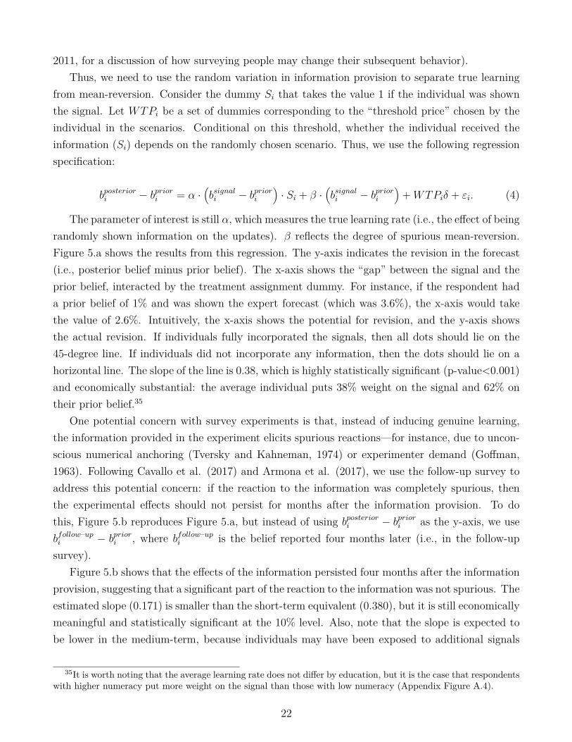
2011, for a discussion of how surveying people may change their subsequent behavior).Thus, we need to use the random variation in information provision to separate true learning

from mean-reversion. Consider the dummy Si that takes the value 1 if the individual was shownthe signal. Let WTPi be a set of dummies corresponding to the “threshold price” chosen by theindividual in the scenarios. Conditional on this threshold, whether the individual received theinformation (Si) depends on the randomly chosen scenario. Thus, we use the following regressionspecification:

bposteriori − bpriori = α ·(bsignali − bpriori

)· Si + β ·

(bsignali − bpriori

)+WTPiδ + εi. (4)

The parameter of interest is still α, which measures the true learning rate (i.e., the effect of beingrandomly shown information on the updates). β reflects the degree of spurious mean-reversion.Figure 5.a shows the results from this regression. The y-axis indicates the revision in the forecast(i.e., posterior belief minus prior belief). The x-axis shows the “gap” between the signal and theprior belief, interacted by the treatment assignment dummy. For instance, if the respondent hada prior belief of 1% and was shown the expert forecast (which was 3.6%), the x-axis would takethe value of 2.6%. Intuitively, the x-axis shows the potential for revision, and the y-axis showsthe actual revision. If individuals fully incorporated the signals, then all dots should lie on the45-degree line. If individuals did not incorporate any information, then the dots should lie on ahorizontal line. The slope of the line is 0.38, which is highly statistically significant (p-value<0.001)and economically substantial: the average individual puts 38% weight on the signal and 62% ontheir prior belief.35

One potential concern with survey experiments is that, instead of inducing genuine learning,the information provided in the experiment elicits spurious reactions—for instance, due to uncon-scious numerical anchoring (Tversky and Kahneman, 1974) or experimenter demand (Goffman,1963). Following Cavallo et al. (2017) and Armona et al. (2017), we use the follow-up survey toaddress this potential concern: if the reaction to the information was completely spurious, thenthe experimental effects should not persist for months after the information provision. To dothis, Figure 5.b reproduces Figure 5.a, but instead of using bposteriori − bpriori as the y-axis, we usebfollow–upi − bpriori , where bfollow–upi is the belief reported four months later (i.e., in the follow-upsurvey).

Figure 5.b shows that the effects of the information persisted four months after the informationprovision, suggesting that a significant part of the reaction to the information was not spurious. Theestimated slope (0.171) is smaller than the short-term equivalent (0.380), but it is still economicallymeaningful and statistically significant at the 10% level. Also, note that the slope is expected tobe lower in the medium-term, because individuals may have been exposed to additional signals

35It is worth noting that the average learning rate does not differ by education, but it is the case that respondentswith higher numeracy put more weight on the signal than those with low numeracy (Appendix Figure A.4).

22

during the interim four months, thus gradually diluting the effect of the signal provided duringour experiment.

Figure 6.a investigates whether the learning rates differ across the three pieces of information.Ex ante, there is little reason for rates to differ: once respondents reveal their information prefer-ence, they should be equally responsive to it. This is confirmed in the figure. Panels b and c ofFigure 6 investigate whether the learning rate differs by WTP for information or by uncertaintyin prior belief. Under Bayesian updating, respondents who were more uncertain should have putmore weight on the signal. Likewise, individuals who valued the information more arguably shouldhave put more weight on it. While we do not find evidence of differential learning for high vs. lowWTP respondents, we see from panel c that respondents with higher prior uncertainty, if anything,tend to update less. Our next result thus is as follows:

Result 3 : Respondents incorporate information that they buy, and the weight that re-spondents put on the information does not vary by information type. However, contraryto rational updating, we do not find the weight to be higher for individuals with higherprior uncertainty.

3.4 Hypothesis 4: Information Acquisition and Dispersion of Expec-tations

In this subsection, we study how information acquisition affects dispersion in beliefs. We beginby investigating the effect of an exogenous reduction in the cost of information. In Stage 3, ascenario is picked at random. Thus, the experimental setup induces exogenous variation in thecost of information. We exploit this and compare how beliefs evolve when “low-price” ($0.01–$1.5)scenarios are picked at random, versus “high-price” ($2–$5) scenarios. Table 5 presents the resultsfrom this test. First of all, notice from the first row of the table that the lower cost of informationdid result in more information acquisition: the share of individuals acquiring information is 21percentage points higher in the low-price group relative to the high-price group.

The rest of the rows from Table 5 show how beliefs evolved for the low- and high-price groups.As expected (due to the scenario being picked at random), the distribution of prior beliefs for thetwo groups is similar. At the final stage, due to the belief updating of those who saw the signal(as studied above), the mean forecast increased and uncertainty decreased. However, even thougha significantly higher share of respondents in the low-price group saw a signal, the dispersion inbeliefs remains similar across the two groups. In particular, we do not find evidence that the meanabsolute deviation (MAD) is lower for the low-price group: in fact, it is slightly higher, at 2.21,than for the high-price group, which has a mean absolute deviation of 2.13 (the difference is notstatistically significant at conventional levels; p-value=0.59).

We also study an additional measure of disagreement, defined as follows: for each respondent,we construct a 95% confidence interval for their forecast based on their point forecast along with

23

the reported uncertainty.36 We then form all possible pairs of respondents within a group (here,the low-price and high-price groups) and define a disagreement as occurring for a pair if the tworespondents’ constructed confidence intervals do not overlap. This measure thus reflects effectsof information both on the dispersion in point forecasts and on respondents’ uncertainty. InTable 5, we see that the fraction of disagreements roughly doubled from the prior stage to theposterior stage, primarily because respondents’ uncertainty went down. However, we again seethat disagreement is almost exactly at the same level for the group with a low cost of information,which was much more likely to obtain the signal, than for the group with a high cost of information.

How is it that more information does not induce higher consensus? Figures 7 and 8 explore thisquestion. Figure 7 shows the distribution of prior beliefs for individuals who were not shown theinformation (Figure 7.a) versus individuals who were shown the information (Figure 7.b). Com-paring the two indicates that these two groups started with similar distributions of beliefs. Figure8 shows the comparison of posterior beliefs between individuals who were not shown information(Figure 8.a) versus individuals who were shown the information (Figure 8.b). Figure 8.a showsthat, among individuals who were not shown information, the distribution of posterior beliefs isthe same regardless of whether the individuals preferred the expert forecast, past-one-year homeprice change, or past-ten-year home price change.37 In contrast, Figure 8.b shows that, for indi-viduals who saw the information, posterior beliefs were substantially different across the threeinformation groups. In each group, posterior beliefs moved towards the values of the respectivesignals: that is, -0.1% for the ten-year price change, 3.6% for the expert forecast, and 6.8% for theone-year price change. Within a group, the revelation of information tended to decrease dispersionof expectations. However, because those groups moved towards differing signals, the dispersionin beliefs across those three groups increased. The net effect of information acquisition on beliefdispersion depends on the combination of these two channels, which end up canceling each otherout.

Table 6 provides a more quantitative version of the previous graphical argument. The first twocolumns of Table 6 describe prior and posterior beliefs, respectively. It is worth remembering thatwhether or not a respondent sees information is endogenous to their WTP, which in turn mayreflect other characteristics. Therefore, the comparison here is not as “clean” as the one in Table5, which relies on experiment-induced variation in whether a respondent saw the information.

We are primarily interested in one feature of these beliefs: the dispersion, measured by themean absolute deviation (MAD) across individuals. The first thing that we can corroborate isthat, within information groups, information provision tended to reduce belief dispersion (but

36Note that our results are qualitatively unchanged if we use confidence intervals with different coverage, e.g.90% or 50%.

37Consistent with the evidence discussed above that subjects in the no-information group may have searchedfor information or thought harder about the question, a comparison of Figure 7.a versus Figure 8.a indicates thatthe distribution of beliefs changed from prior to posterior even for individuals who were not shown information(p<0.01, MWW test).

24

belief dispersion remained high). For instance, for individuals who preferred the forecast and wereshown the information, the MAD decreased from 2.19 to 1.14 percentage points. In contrast,for individuals who preferred the expert forecast but did not get to see the information, theMAD in beliefs increased from 1.93 percentage points for prior beliefs to 2.38 for posterior beliefs.These qualitative differences are consistent inside the group of individuals who chose the 10-yearinformation, while for those who chose the 1-year information, MAD even increased for those whosaw the info (perhaps because the signal was rather “extreme”), though less so than for those whodid not see the info.

Now we turn to the sample that pools the individuals across all three information sources. Inthis pooled sample, the group that saw the information did not see a decline in the mean absolutedeviation of beliefs: this measure of dispersion is 2.04 percentage points for the prior beliefs and2.05 percentage points for the posterior beliefs.38 And since respondents became more confident intheir forecast, disagreement substantially increases, from 10.7% to 19.7% of all pairs. Disagreementalso increases, though somewhat less strongly, in the no-information group; the difference-in-differences across groups is not statistically significant. Regarding confidence in expectations,mean uncertainty in posterior beliefs is lower than that in prior beliefs for both groups (those whosaw the information and those who did not). However, consistent with the notion that informationshould make individuals more certain, we see that uncertainty declines more for the group that isshown information (from 3.9 to 2.8 percentage points, or more than 1 percentage point) than forthe group that is not shown information (from 4.1 to 3.6 percentage points).

The table also shows how the cross-sectional dispersion evolves in the medium term. Ex-ante,the medium-term impact on dispersion is unclear – in the interim four months, individuals mayhave received various signals. Depending on the heterogeneity in these signals, the cross-sectionaldispersion may go up or down. Additionally, because individuals are being asked about year-end home prices, some uncertainty may have resolved over the interim four months. The lastcolumn in Table 6 shows how these statistics evolved for the information-shown and not-showngroups. Comparing the follow-up belief with the posterior belief, the mean absolute deviation inexpectations increases for both the information-shown and not-shown groups, though somewhatmore so for the former group, which also sees a slight increase in disagreement.

One potential concern is that the cross-sectional dispersion does not decrease when informationis cheaper just because respondents could buy, at most, one of the three information pieces. Couldallowing individuals to view multiple pieces of information reverse this result? To investigate this,we fielded a supplementary module in the 2018 SCE Housing Survey. Details of this module andthe analysis are presented in Appendix B. In this supplementary study, respondents can choosebetween two pieces of information. Then, we randomize them into three groups: they get to observeeither no information, their preferred information, or both pieces of information. The comparison

38The mean absolute deviation in the pooled sample that does not see information does go up (from 2.27 to2.61), but that difference is statistically insignificant (p-value=0.15).

25

between no information and their preferred information is equivalent to the comparison from themain experiment (i.e., randomizing the price of the preferred information between zero or infinity).We corroborate the finding from the main survey: cross-sectional dispersion does not decline whensubjects get to see either their preferred information or both pieces of information. We find thatrandomly providing two signals at the same time has effects similar to providing just one piece ofinformation, and that cross-sectional dispersion (measured either by the MAD or the disagreementmetric) does not go down.

The fourth set of findings can be summarized as follows:

Result 4 : A lower cost of information does not lead to a decrease in the cross-sectionaldispersion of beliefs. This finding arises for two reasons. First, individuals chooseto acquire different pieces of information and put significant weight on the acquiredinformation. Second, within groups of individuals who acquire the same information,dispersion in beliefs remains high.

4 Theory

We present a simple model that can match most of the experimental findings. The model is acombination of a sticky information model, as in Reis (2006), and a rational inattention model, asin Sims (2003). The model also features heterogeneous prior beliefs about the quality of differentinformation sources.

4.1 Model

The timing is as follows:

1. Individuals report their prior beliefs over the fundamental.

2. Individuals can acquire access to one of three information sources at cost c or no information(“information acquisition”).

3. The selected information is displayed and individuals choose the amount of attention allo-cated to the displayed information (“information processing”).

4. Individuals report posterior beliefs over the fundamental and receive a payoff.

Individual i has the prior belief that the fundamental θ is normally distributed with mean µθ (i)and variance σ2

θ (i), where the i indicates that the prior belief over the fundamental may differacross individuals. In the experiment, the fundamental is house price growth during the calendaryear.

26

Individuals have the common prior belief that each information source j ∈ 1, 2, 3 is a noisysignal on the fundamental

xj = θ + εj,

where xj is the displayed information and the noise εj is normally distributed with mean zero,but individuals may have heterogeneous prior beliefs over precisions. Individual i believes thatthe precisions of the three information sources equal τ1 (i) ≡ (1/σ2

ε,1 (i)), τ2 (i) ≡ (1/σ2ε,2 (i)), and

τ3 (i) ≡ (1/σ2ε,3 (i)), where the i indicates that the prior belief over precisions may differ across

individuals. In the appendix, we solve a model with a common prior belief over precisions. In thatmodel, individuals can process information about precisions before selecting an information source.Heterogeneity in beliefs over precisions arises ex post due to idiosyncratic processing mistakes. Inthat model, additional features of the experimental data arise endogenously. Here we focus onthe simpler model with heterogeneous priors over precisions and no information processing beforeselecting an information source.

If an individual acquires access to an information source, the information is displayed. Payingattention to this information is modeled as a noisy signal on the displayed information

s (i) = xj + ψ (i) ,

where j is the information source that the individual selected, xj is the displayed information, andψ (i) is noise that arises due to limited attention to the displayed information. That is, limitedattention creates a noisy perception of the displayed information. The noise ψ (i) is assumed to benormally distributed with mean zero and variance σ2

ψ (i). Paying more attention to the displayedinformation is formalized as a smaller variance of noise, σ2

ψ (i). Individuals choose the amount ofattention allocated to the displayed information, i.e., they choose σ2

ψ (i).Posterior beliefs follow from Bayesian updating. If individual i selected information source

j ∈ 1, 2, 3 and chose the variance of noise σ2ψ (i), her posterior belief is given by combining her

prior belief with the signals (i) = θ + εj + ψ (i) .

The posterior mean of the fundamental is

E [θ|s (i)] = µθ (i) + σ2θ (i)

σ2θ (i) + σ2

ε,j (i) + σ2ψ (i) [θ + εj + ψ (i)− µθ (i)] . (5)

The weight on the displayed information is an increasing function of the perceived precision ofthe selected information source and the attention allocated to the displayed information.39 The

39In Gabaix’s (2014) model of sparsity, the weight on information is also an increasing function of attention tothe information, as in Sims’ (2003) model of rational inattention. One difference between these theories is that inSims’ (2003) model of rational inattention the weight on information can be viewed as the optimal response to anoisy perception of the information. The noisy perception of information in turn helps to match heterogeneity in

27

posterior variance of the fundamental is

σ2θ|s (i) = 1

1σ2θ(i) + 1

σ2ε,j(i)+σ

2ψ

(i).

The payoff received by individual i at the end equals

−φ (θ − E [θ|s (i)])2 ,

where the parameter φ controls the incentive to have an accurate posterior.The optimal information strategy of an individual consists of an acquisition strategy (j ∈

1, 2, 3 or no information) and an attention strategy (σ−2ψ (i) ≥ 0) that maximize the expected

payoff net of the costs of acquiring and processing information:

−φσ2θ|s (i)− cz − d

(σ−2ψ (i)

),

where c is the cost of acquiring information, z is an indicator variable which takes the value oneif information is acquired, and d

(σ−2ψ (i)

)denotes the cost of paying attention to the displayed

information. One can think of the cost c as the sticky information aspect of the model (Mankiwand Reis, 2002), because in micro-founded versions of sticky information models there is a fixedcost of acquiring information (Reis, 2006).

Following Sims (2003), the cost of paying attention to displayed information is assumed to bean increasing function f of the uncertainty reduction about the displayed information

d(σ−2ψ (i)

)= f (H (xj)−H (xj|s (i))) ,

where H (xj) denotes the entropy of displayed information and H (xj|s (i)) denotes the conditionalentropy of the displayed information given the signal on the displayed information. Since entropyis simply a measure of uncertainty, the argument of the function f simply measures the uncertaintyreduction about the displayed information due to the signal on the displayed information. Theentropy of a normally distributed random variable x with variance σ2

x equals a constant plus12 ln (σ2

x), and hence, the last equation reduces to

d(σ−2ψ (i)

)= f

12 ln

σ2x,j (i)

σ2x,j|s (i)

= f

12 ln

σ2x,j (i)

σ2x,j(i)σ

2ψ

(i)σ2x,j(i)+σ

2ψ

(i)

= f

(12 ln

(1 +

σ2x,j (i)σ2ψ (i)

)).

The cost of paying attention to displayed information is an increasing function of the signal-to-noiseratio in the signal on the displayed information. In the rational inattention literature following

reported posterior beliefs among individuals who see the same information.

28

Sims (2003), it is quite common to assume that f is a linear function, in which case the lastequation reduces to

d(σ−2ψ (i)

)= µ

12 ln

(1 +

σ2x,j (i)σ2ψ (i)

),

where µ > 0 denotes the marginal cost of attention. All results presented in the following subsectionalso hold for any function f that is strictly increasing, convex, twice continuously differentiable,and has a non-zero derivative at zero.

4.2 Solution and comparison to experimental findings

The following proposition characterizes the solution to the model.

Proposition 1 Individual i’s optimal information strategy is to select the information source ofthe highest perceived precision,

j∗ (i) = arg maxj∈1,2,3

(1

σ2ε,j (i)

),

and to choose the precision of the signal on the displayed information that maximizes the net benefitof paying attention to the displayed information:

1σ2,∗ψ (i)

= arg max(1/σ2

ψ(i))≥0

φσ2

θ (i)− 11

σ2θ(i) + 1

σ2ε,j∗ (i)+σ2

ψ(i)

− µ

2 ln(

1 +σ2θ (i) + σ2

ε,j∗ (i)σ2ψ (i)

) . (6)

More attention yields a more accurate posterior but is also more costly. If the willingness to payfor access to the preferred information source (the max in (2)) exceeds the cost c, the individualacquires access to the preferred information source and the posterior mean of the fundamental isgiven by equation (1) with j = j∗ (i) and σ2

ψ (i) = σ2,∗ψ (i).

The maximization problem (2) has the following properties. First, there exists a unique solution.Second, for sufficiently low φ/µ, high σ−2

θ (i), and low σ−2ε,j∗ (i), the solution is a corner solution.

In this case, it is optimal to pay no attention to the displayed information and the willingness topay for access to the information therefore equals zero. Third, in the case of an interior solution,the optimal precision σ−2,∗

ψ (i) is strictly increasing in φ/µ and σ−2ε,j∗ (i).

Before turning to a comparison of model predictions and experimental findings, we make threeassumptions about heterogeneity.

Assumption 1: There is cross-sectional heterogeneity in arg maxj∈1,2,3

(1

σ2ε,j(i)

).

Assumption 2: There is cross-sectional heterogeneity in the marginal cost of attention µ, andthe marginal cost of attention µ is negatively correlated with numeracy in the cross section. Thisassumption seems natural since individuals with higher numeracy presumably find it less costly topay attention to quantitative information and all displayed information is quantitative information.

29

Assumption 3: There is cross-sectional heterogeneity in the taste for information φ, and theprecision of the prior σ−2

θ (i) is positively correlated with the taste for information φ in the crosssection. This assumption also seems natural because experimental subjects had the possibility toacquire and process information already before the experiment.

Finally, we compare model predictions and experimental findings.First, due to corner solutions in the allocation of attention, the model can match the exper-

imental finding that some individuals choose to acquire no information even before learning thecost of information acquisition. There is no point in acquiring information that one will not payattention to anyway.

Second, with heterogeneous priors over precisions (Assumption 1), the model can match theexperimental finding that individuals select different information sources. Furthermore, the factthat the average willingness to pay and the average weight on the displayed information do not differacross the three information groups suggests that max

j∈1,2,3

(1

σ2ε,j(i)

)does not differ systematically

across the three information groups. That is, individuals rank information sources differently butthink equally highly of their preferred information source.

Third, the model can match the experimental finding that individuals in the higher-rewardtreatment have a higher willingness to pay and thus are more likely to acquire the information.

Fourth, with costly attention (µ > 0), the model can match the experimental finding thatnumeracy and reward matter conditional on information being displayed. Under Assumption 2the model can match the experimental finding that individuals with higher numeracy react moreto the displayed information (because they pay more attention to the displayed information) andthe experimental finding that they select the alternative “I would not like to see any information”less frequently (because the optimal allocation of attention is less likely to be a corner solution).Under Assumption 3 the model can match the experimental finding that individuals with higherprecision of the prior react more to the displayed information. Bayesian updating implies thatagents with higher precision of the prior put a smaller weight on the signal. Endogenous attentionimplies that agents with a stronger taste for information pay more attention to the displayedinformation, implying a larger weight on the signal. Hence, if the precision of the prior and φ arepositively correlated in the cross section, individuals with higher precision of the prior may end upputting a larger weight on the signal. Furthermore, the model can match the experimental findingthat individuals in the higher-reward treatment spend more time on processing the displayedinformation.

Fifth, Bayesian updating under rational information acquisition and rational inattention impliesthat individuals with strictly positive willingness to pay put a strictly positive weight on the signal.A strictly positive willingness to pay implies that the preferred information source is perceivedto be useful and the individual plans to pay attention to the displayed information, which inturn implies that the weight on the signal is strictly positive. Hence, the posterior beliefs ofindividuals who acquire access to different information sources should diverge, which matches

30

the experimental finding that the posterior beliefs of individuals who select different informationsources move towards different signals. Finally, within a group, access to the information sourcedecreases dispersion in beliefs if and only if the fact that individuals put weight on the samedisplayed information dominates the fact that there is individual-specific noise in the signal onthe displayed information and the fact that individuals may have heterogeneous signal weights.Thus, the model can also match the experimental finding that dispersion in beliefs falls withinsome groups and increases within other groups once information is displayed.40

Table 7 summarizes the predictions of the following versions of the model: (i) common prior overprecisions and costless attention, (ii) heterogeneous priors over precisions and costless attention,(iii) heterogeneous priors over precisions and costly attention. These predictions hold for any levelof the cost of information acquisition, c ≥ 0. In sum, the special case of the model with a commonprior over precisions and costless attention can match only a small subset of the findings. Thebenchmark version of the model with heterogeneous priors over precisions and costly attention canmatch almost all of the findings.

In the appendix, we solve a model where we replace the assumption of heterogeneous priorsover precisions by the assumption of a common prior over precisions and the assumption thatindividuals can process information about the quality of information sources before selecting aninformation source. Heterogeneity in beliefs over precisions arises ex post due to idiosyncraticinformation-processing mistakes. In that model, additional features of the experimental data ariseendogenously. In particular, the highest-precision information source is endogenously the modalchoice, and under Assumption 2, high numeracy individuals are endogenously more likely to selectthe highest-precision information source.

5 Discussion and Conclusion

Using an innovative experimental setup that makes the information acquisition process endogenous,this paper attempts to understand the role of information frictions in explaining the heterogeneityin consumers’ expectations about home price changes. Consumers exhibit substantial demand forinformation and, consistent with rational inattention, the demand for information is high when thestakes are high. Although information acquisition costs do seem to matter, our findings indicatethat the main drivers of heterogeneity in consumer expectations are constraints on informationprocessing. Consumers disagree on what information is most informative, with less sophisticatedagents less likely to choose “informative” signals. Importantly, we see that the cross-sectionalvariance of the expectations distribution does not decrease because of endogenous information

40In the literature on noisy rational expectations models of financial markets following Grossman and Stiglitz(1980), there also exist models in which heterogeneity in beliefs arises because agents select different pieces ofinformation. However, in that literature, agents select different pieces of information because equilibrium pricespartially reveal information, while here agents select different pieces of information because of heterogeneity inbeliefs over precisions.

31

acquisition, which would be expected in a setting with rational acquisition and information pro-cessing.

Endogenous information acquisition may thus increase disagreement across individuals, eventhough the opinions of people who look at the same signals tend to converge. Disagreementis thought to be an important driver of trade in asset markets (e.g. Harrison and Kreps 1978,Scheinkman and Xiong 2003, Hong and Stein 2007). In the context of the housing market, Baileyet al. (2017) show that counties with higher disagreement (which in their case is driven by differenthouse price experiences of out-of-town friends) see higher trading volumes. Thus, to the extentthat different households vary in the information sources they rely on, as our evidence suggests,differing signals from these sources may have important consequences for activity and prices in thehousing market.

On the modeling front, many models with information frictions assume that individuals processinformation in a rational way. Our results suggest that this may be a misleading assumption andinstead support models wherein consumers have heterogeneous beliefs about the precision of in-formation sources, and have limited information processing capacity and process information at afinite rate (e.g., Sims, 2003). In that sense, our conclusion is similar to Coibion and Gorodnichenko(2012) who find that noisy information models are better at characterizing the expectations forma-tion process. Our findings also suggest that consumers may not know which pieces of informationto choose. In fact, we find that less sophisticated individuals (as proxied by education or numer-acy) are less likely to pick informative signals. Thus, our results help explain why consumers tendto have so much dispersion in their expectations.

Disagreement in (inflation) expectations has been shown to vary over time, and the levels tendto be larger among consumers than among experts. For instance, Mankiw, Reis and Wolfers (2003)try to explain this finding through the lens of a sticky-information model, where some people formexpectations based on outdated information. While their model can fit the survey data better thanmodels of rational expectations, it is unable to match other features of the data, such as the positiverelationship between the level of inflation and disagreement in expectations, or the higher level ofdisagreement during recessions. Our findings offer an alternative potential explanation for thesepatterns: consumers all update at regular frequencies but simply look at different information.Future work that tries to understand the dynamics of information acquisition would be valuable.With that goal in mind, it seems important that, in addition to collecting survey measures ofexpectations, we start collecting high-frequency data on the information sources that consumersare paying attention to.

We show that a rational inattention model with heterogeneity amongst consumers in the costof attention and in beliefs about precision of information sources best characterizes our empiricalresults. Besides its implications for modeling of expectation formation, our findings have somedirect policy implications. There is a debate in the literature about the optimal level of informa-tion disclosure by government agencies such as central banks and statistics agencies. For instance,

32

most government agencies have the choice of releasing data such as official statistics on inflation,unemployment, and gross domestic product, among others. Some authors have argued that infor-mation disclosure is optimal (Hellwig 2005), whereas others argue that it can be harmful (Morrisand Shin 2002). These models always assume that individuals process all the available informa-tion optimally. Implicitly, these models are assuming that more information cannot be worse forconsumers, in the sense that that they can choose to ignore bad signals. Our evidence indicatesthat this assumption may be heroic. Instead, our findings imply that it is especially importantfor the government (and, for that matter, non-government) entities to disclose the information ina careful manner. Policy makers may want to act paternalistically by disclosing only the “goodsignals,” by making the best signals more salient, or by guiding the customers on how to interpretand weigh all the available information.

33

References[1] Allcott, H. (2011). “Social Norms and Energy Conservation.” Journal of Public Economics, Vol.

95(9-10), pp. 1082-1095.

[2] Allcott, H., and Kessler, J. B. (2015). “The welfare effects of nudges: A case study of energy usesocial comparisons,” NBER Working Paper No. 21671.

[3] Andersen, S., Harrison, G. W., Lau, M. I., and Rutström, E. E. (2006). “Elicitation using multipleprice list formats”. Experimental Economics, Vol. 9(4), pp. 383-405.

[4] Angulo, A. M., Gil, J. M., and Tamburo, L. (2005). “Food safety and consumers’ willingness to payfor labelled beef in Spain”. Journal of Food Products Marketing, Vol. 11(3), pp. 89-105.

[5] Armantier, O., Nelson, S., Topa, G., van der Klaauw, W. and Zafar, B. (2016). “The Price Is Right:Updating of Inflation Expectations in a Randomized Price Information Experiment,” Review ofEconomics and Statistics, forthcoming.

[6] Armona, L., A. Fuster, B. Zafar (2017). “Home Price Expectations and Behavior: Evidence from aRandomized Information Experiment,” Review of Economic Studies, forthcoming.

[7] Bailey, M., R. Cao, T. Kuchler, and J. Stroebel (2017). “Social Networks and Housing Markets,”NBER Working Paper No. 22258.

[8] Bailey, M., R. Cao, T. Kuchler, and J. Stroebel (2018). “The Economic Effects of Social Networks:Evidence from the Housing Market,” Journal of Political Economy, forthcoming.

[9] Bartoš, V.; Bauer, M.; Chytilová, J.; Matějka, F. (2016). “Attention Discrimination: Theory andField Experiments with Monitoring Information Acquisition,” American Economic Review, Vol.106(6), pp. 1437-1475.

[10] Burke, M., and M. Manz (2014). “Economic literacy and inflation expectations: evidence from aneconomic experiment,” Journal of Money, Credit, and Banking, Vol. 46(7), pp. 1421-1456.

[11] Bordalo, P.; N. Gennaioli, and A. Shleifer (2018). “Diagnostic Expectations and Credit Cycles,”Journal of Finance, forthcoming.

[12] Carroll, C. (2003). “Macroeconomic Expectations of Households and Professional Forecasters,” Quar-terly Journal of Economics, Vol. 118(1), pp. 269-298.

[13] Case, K. and R. Shiller (1989). “The Efficiency of the Market for Single-Family Homes,” AmericanEconomic Review, Vol 79(1), pp. 125–137.

[14] Cavallo, A.; Cruces, G. and Perez-Truglia, R. (2016), “Learning from Potentially Biased Statistics,”Brookings Papers on Economic Activity, Spring 2016, pp. 59–108.

34

[15] Cavallo, A.; Cruces, G. and Perez-Truglia, R. (2017). “Inflation Expectations, Learning and Super-market Prices: Evidence from Survey Experiments,” American Economic Journal: Macroeconomics,Vol 9(3), pp. 1–35.

[16] Cheng, I. and A. Hsiaw (2017). “Distrust in Experts and the Origins of Disagreement.” WorkingPaper.

[17] Coibion, O. and Gorodnichenko, Y. (2012). “What can survey forecasts tell us about informationalrigidities?” Journal of Political Economy, Vol. 120, pp. 116-159.

[18] Coibion, O., Gorodnichenko, Y. and Kumar, S. (2015). “How Do Firms Form Their Expectations?New Survey Evidence.” NBER Working Paper No. 21092.

[19] Cruces, G., Perez-Truglia, R. and Tetaz, Martin (2013). “Biased Perceptions of Income Distribu-tion and Preferences for Redistribution: Evidence from a Survey Experiment”. Journal of PublicEconomics, Vol 98, pp. 100-112.

[20] Cullen, Z. and Perez-Truglia, R. (2017). “How Much Does Your Boss Make? The Effects of SalaryComparisons,” Working Paper.

[21] Duflo, E. and Saez, E. (2003). “The role of information and social interactions in retirement plandecisions: evidence from a randomized experiment,” Quarterly Journal of Economics, Vol 118(3),pp. 815-842.

[22] Fuster, A., B. Hebert, and D. Laibson (2012). “Natural expectations, macroeconomic dynamics, andasset pricing,” NBER Macroeconomics Annual, Vol 26 (1), pp. 1-48.

[23] Gabaix, X. (2017). “Behavioral Inattention,” NBER Working Paper No. 24096.

[24] Gabaix, X.; Laibson, D.; Moloche, G. and Weinberg, S. (2006). “Costly Information Acquisition:Experimental Analysis of a Boundedly Rational Model,” American Economic Review, Vol 96(4),pp.1043-1068.

[25] Glaeser, E., and C. Nathanson. (2015). “Housing Bubbles,” in Handbook of Regional and UrbanEconomics, Volume 5. Eds. Gilles Duranton, Vernon Henderson, and William Strange. 701-751.

[26] Goffman, E. 1963. Stigma: Notes on the Management of Spoiled Identity. Englewood Cliffs, NJ:Prentice-Hall.

[27] Guren, A. (2016): “House Price Momentum and Strategic Complementarity,” Journal of PoliticalEconomy, forthcoming

[28] Harrison, J.M. and D.M. Kreps (1978). “Speculative investor behavior in a stock market with het-erogeneous expectations,” Quarterly Journal of Economics, Vol 92(2): 323–336.

[29] Hellwig, C. (2005). “Heterogeneous Information and the Welfare Effects of Public Information Dis-closures.” UCLA Economics Working Paper No. 283.

35

[30] Hoffman, M. (2016). “How is Information Valued? Evidence from Framed Field Experiments.” TheEconomic Journal, Vol 126(595): 1884-1911.

[31] Hong, H. and J.C. Stein (2007). “Disagreement and the stock market,” Journal of Economic Per-spectives, Vol 21(2): 109–128.

[32] Hoopes, J.; Reck, D. and Slemrod, J. (2015). “Taxpayer Search for Information: Implications forRational Attention,” American Economic Journal: Economic Policy, Vol 7(3), pp. 177-208.

[33] Khattak, A. J., Yim, Y., and Prokopy, L. S. (2003). “Willingness to pay for travel information,”Transportation Research Part C: Emerging Technologies, Vol 11(2), pp. 137-159.

[34] Laster, D., Bennett, P., and Geoum, I. S. (1999). “Rational Bias in Macroeconomic Forecasts,” TheQuarterly Journal of Economics, Vol 114(1), pp. 293-318.

[35] Maćkowiak, B., and Wiederholt, M. (2009). “Optimal sticky prices under rational inattention,” TheAmerican Economic Review, Vol 99(3), pp. 769-803.

[36] Malmendier, U. and Nagel, S. (2016). “Learning from Inflation Experiences,” The Quarterly Journalof Economics, Vol 131(1), pp. 53-87.

[37] Mankiw, N.G. and Reis, R. (2002). “Sticky Information Versus Sticky Prices: A Proposal To ReplaceThe New Keynesian Phillips Curve,” Quarterly Journal of Economics, Vol 117(4), pp. 1295-1328.

[38] Mankiw, N.G., Reis, R. and Wolfers, J. (2003). “Disagreement About Inflation Expectations.” InNBER Macroeconomics Annual 2003, ed. by M. Gertler, and K. Rogoff.

[39] Morris, S. and H.S. Shin (2002). “The Social Value of Public Information,” American EconomicReview, Vol. 92 (5), pp. 1521–34.

[40] Mullainathan, S. and A. Shleifer. (2005). “The Market for News,” American Economic Review, Vol95(4), pp. 1031-1053.

[41] Reis, R. (2006). “Inattentive consumers,” Journal of monetary Economics, Vol 53(8), pp. 1761-1800.

[42] Scheinkman, J.A andW. Xiong (2003). “Overconfidence and speculative bubbles,” Journal of PoliticalEconomy, Vol 111(6), pp. 183–1220.

[43] Shiller, R. (2005). “Irrational Exuberance,” Second Edition, Princeton: Princeton University Press.

[44] Silverman, D.; J. Slemrod and N. Uler (2014). “Distinguishing the Role of Authority ’In’ and Au-thority ’To’,” Journal of Public Economics, Vol 113, pp. 32-42.

[45] Sims, C. (2003). “Implications of rational inattention,” Journal of monetary Economics, Vol 50(3),pp. 665-690.

[46] Tversky, A. and D. Kahneman. 1974. “Judgment under Uncertainty: Heuristics and Biases.” Science185 (4157): 1124–31.

36

[47] Wiswall, M., and B. Zafar. (2015). “Determinants of College Major Choices: Identification from anInformation Experiment.” Review of Economic Studies, Vol 82(2), pp. 791-824.

[48] Woodford, M. (2003). “Imperfect Common Knowledge and the Effects of Monetary Policy,” In Knowl-edge, Information, and Expectations in Modern Macroeconomics: In Honor of Edmund Phelps, editedby P. Aghion, R. Frydman, J. Stiglitz, and M. Woodford. Princeton, NJ: Princeton Univ. Press.

[49] Zwane, A.; Zinman, J.; Van Dusen, E.; Pariente, W.; Null, C.; Miguel, E.; Kremer, M.; Karlan, D.;Hornbeck, R.; Gine, X.; Duflo, E.; Devoto, F.; Crepon, B. and Banerje, A. (2011). “Being surveyedcan change later behavior and related parameter estimates,” Proceedings of the National Academyof Sciences, Vol 108, pp. 1821–1826.

37

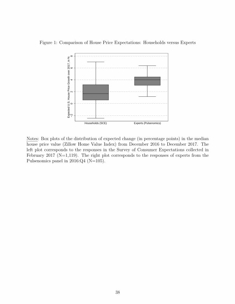
Figure 1: Comparison of House Price Expectations: Households versus Experts

−2

02

46

8E

xpec

ted

U.S

. Hou

se P

rice

Gro

wth

ove

r 20

17, i

n %

Households (SCE) Experts (Pulsenomics)

Notes: Box plots of the distribution of expected change (in percentage points) in the medianhouse price value (Zillow Home Value Index) from December 2016 to December 2017. Theleft plot corresponds to the responses in the Survey of Consumer Expectations collected inFebruary 2017 (N=1,119). The right plot corresponds to the responses of experts from thePulsenomics panel in 2016:Q4 (N=105).

38

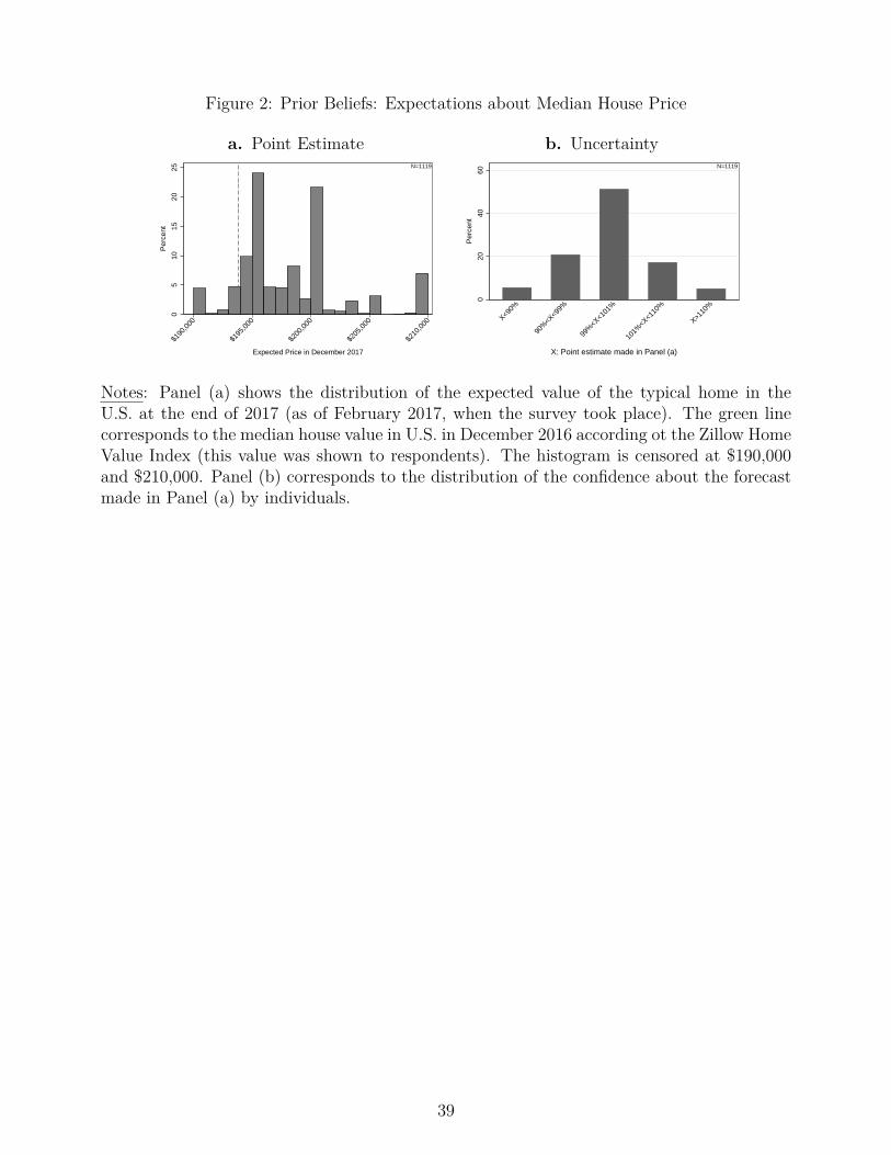
Figure 2: Prior Beliefs: Expectations about Median House Price

a. Point Estimate b. Uncertainty0

510

1520

25

Per

cent

$190

,000

$195

,000

$200

,000

$205

,000

$210

,000

Expected Price in December 2017

N=1119

020

4060

Per

cent

X<90%

90%

<X<9

9%

99%

<X<1

01%

101%

<X<1

10%

X>110

%

X: Point estimate made in Panel (a)

N=1119

Notes: Panel (a) shows the distribution of the expected value of the typical home in theU.S. at the end of 2017 (as of February 2017, when the survey took place). The green linecorresponds to the median house value in U.S. in December 2016 according ot the Zillow HomeValue Index (this value was shown to respondents). The histogram is censored at $190,000and $210,000. Panel (b) corresponds to the distribution of the confidence about the forecastmade in Panel (a) by individuals.

39

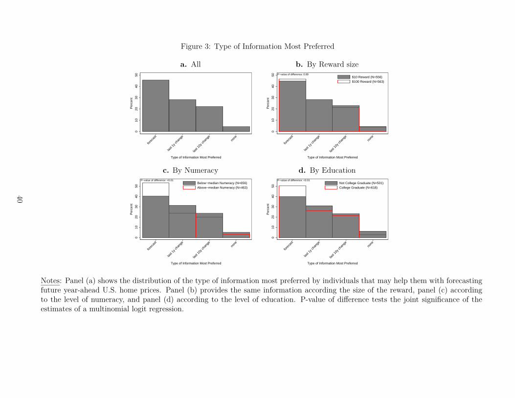
Figure 3: Type of Information Most Preferred

a. All b. By Reward size

010

2030

4050

Per

cent

fore

cast

last 1

y cha

nge

last 1

0y ch

ange

none

Type of Information Most Preferred

010

2030

4050

Per

cent

fore

cast

last 1

y cha

nge

last 1

0y ch

ange

none

Type of Information Most Preferred

$10 Reward (N=556)$100 Reward (N=563)

P−value of difference: 0.89

c. By Numeracy d. By Education

010

2030

4050

Per

cent

fore

cast

last 1

y cha

nge

last 1

0y ch

ange

none

Type of Information Most Preferred

Below−median Numeracy (N=656)Above−median Numeracy (N=463)

P−value of difference: <0.01

010

2030

4050

Per

cent

fore

cast

last 1

y cha

nge

last 1

0y ch

ange

none

Type of Information Most Preferred

Not College Graduate (N=501)College Graduate (N=618)

P−value of difference: <0.01

Notes: Panel (a) shows the distribution of the type of information most preferred by individuals that may help them with forecastingfuture year-ahead U.S. home prices. Panel (b) provides the same information according the size of the reward, panel (c) accordingto the level of numeracy, and panel (d) according to the level of education. P-value of difference tests the joint significance of theestimates of a multinomial logit regression.

40

Figure 4: Willingness to Pay for Favorite Information

a. All b. By Reward Size

010

2030

4050

Per

cent

<=$0

$0−0

.5$0

.5−1

$1−1

.5$1

.5−2

$2−2

.5$2

.5−3

$3−3

.5$3

.5−4

$4−4

.5$4

.5−5 >$

5

Maximum Willingness to Pay for Information

N=1013

010

2030

4050

Per

cent

<=$0

$0−0

.5$0

.5−1

$1−1

.5$1

.5−2

$2−2

.5$2

.5−3

$3−3

.5$3

.5−4

$4−4

.5$4

.5−5 >$

5

Maximum Willingness to Pay for Information

10$ Reward (N=506)100$ Reward (N=507)

P−value of difference: <0.01

c. Forecast vs. 1yr d. Forecast vs. 10yr

010

2030

4050

Per

cent

<=$0

$0−0

.5$0

.5−1

$1−1

.5$1

.5−2

$2−2

.5$2

.5−3

$3−3

.5$3

.5−4

$4−4

.5$4

.5−5 >$

5

Maximum Willingness to Pay for Information

Forecast Information (N=480)1 year Information (N=299)

P−value of difference: 0.44

010

2030

4050

Per

cent

<=$0

$0−0

.5$0

.5−1

$1−1

.5$1

.5−2

$2−2

.5$2

.5−3

$3−3

.5$3

.5−4

$4−4

.5$4

.5−5 >$

5

Maximum Willingness to Pay for Information

Forecast Information (N=480)10 year Information (N=234)

P−value of difference: 0.13

Notes: This sample does not include respondents who chose “None” as their most favorite information source and respondents withnon-monotonic choices across the BDM scenarios. Panel (a) shows the distribution of maximum willingness to pay for favoriteinformation in the whole sample. Panel (b) shows the distribution of maximum willingness to pay for information according the sizeof the reward. Panel (c) compares the distribution of WTP between individuals who preferred forecasts information and individualswho preferred information over the last one year. Panel (d) compares the distribution of WTP between individuals who preferredforecasts information and individuals who preferred information over the last ten years. P-value of difference refers to the Mann-Whitney-Wilcoxon test of the equality of two distributions.

41

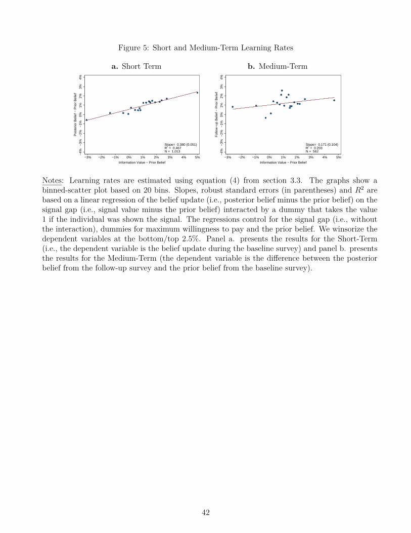
Figure 5: Short and Medium-Term Learning Rates

a. Short Term b. Medium-Term−

4%−

3%−

2%−

1%0%

1%2%

3%4%

Pos

terio

r B

elie

f − P

rior

Bel

ief

−3% −2% −1% 0% 1% 2% 3% 4% 5%

Information Value − Prior Belief

Slope= 0.380 (0.051) R2 = 0.467 N = 1,013

−4%

−3%

−2%

−1%

0%1%

2%3%

4%

Fol

low

−up

Bel

ief −

Prio

r B

elie

f

−3% −2% −1% 0% 1% 2% 3% 4% 5%

Information Value − Prior Belief

Slope= 0.171 (0.104) R2 = 0.203 N = 562

Notes: Learning rates are estimated using equation (4) from section 3.3. The graphs show abinned-scatter plot based on 20 bins. Slopes, robust standard errors (in parentheses) and R2 arebased on a linear regression of the belief update (i.e., posterior belief minus the prior belief) on thesignal gap (i.e., signal value minus the prior belief) interacted by a dummy that takes the value1 if the individual was shown the signal. The regressions control for the signal gap (i.e., withoutthe interaction), dummies for maximum willingness to pay and the prior belief. We winsorize thedependent variables at the bottom/top 2.5%. Panel a. presents the results for the Short-Term(i.e., the dependent variable is the belief update during the baseline survey) and panel b. presentsthe results for the Medium-Term (the dependent variable is the difference between the posteriorbelief from the follow-up survey and the prior belief from the baseline survey).

42

Figure 6: Learning from Feedback

a. By Info Chosen b. By WTP c. By Uncertainty in Priors−

4%−

3%−

2%−

1%0%

1%2%

3%4%

Pos

terio

r B

elie

f − P

rior

Bel

ief

−3% −2% −1% 0% 1% 2% 3% 4% 5%

Information Value − Prior Belief

Forecast (N=480)Last 1 year change (N=299)Last 10 year change (N=234)

SlopeForecast = 0.328 (0.111) Slope1−year = 0.304 (0.092) Slope10−years = 0.305 (0.095)

−4%

−3%

−2%

−1%

0%1%

2%3%

4%

Pos

terio

r B

elie

f − P

rior

Bel

ief

−3% −2% −1% 0% 1% 2% 3% 4% 5%

Information Value − Prior Belief

MWP < $2.5 (N=293)MWP ≥ $2.5 (N=720)

SlopeMWP < $2.5 = 0.358 (0.115) SlopeMWP ≥ $2.5 = 0.366 (0.164)

−4%

−3%

−2%

−1%

0%1%

2%3%

4%

Pos

terio

r B

elie

f − P

rior

Bel

ief

−3% −2% −1% 0% 1% 2% 3% 4% 5%

Information Value − Prior Belief

Below−median uncertainty (N=506)Above−median uncertainty (N=507)

SlopeBelow = 0.471 (0.082) SlopeAbove = 0.328 (0.063)

Notes: This sample does not include respondents who chose “None” as their most favorite information source and respondents withnon-monotonic choices across the BDM scenarios. Learning rates are estimated using equation (4) from section 3.3. The graphs showa binned-scatter plot based on 20 bins. Slopes, robust standard errors (in parentheses) and R2 are based on a linear regression of thebelief update (i.e., the dependent variable is the belief update during the baseline survey) on the signal gap (i.e., signal value minusthe prior belief) interacted by a dummy that takes the value 1 if the individual was shown the signal. The regressions control for thesignal gap (i.e., without the interaction), dummies for maximum willingness to pay and the prior belief. We winsorize the dependentvariables at the bottom/top 2.5%. . Panel a. presents the results according info chosen (i.e., forecast, last 1-year change, and last10-year change). Panel b. presents results according WTP (i.e., above and below the median WTP). Finally, panel c. presents theresults according the uncertainty (i.e., above and below the median uncertainty).

43

Figure 7: Prior Beliefs: Individuals Who Will not be Shown Information vs. Individuals Who Will

a. Information not to be Shown b. Information to be Shown0

2040

60

≤ −1% 0% 1% 2% 3% 4% 5% 6% 7% ≥ 8%

N=123

Information Chosen: Forecast

020

4060

≤ −1% 0% 1% 2% 3% 4% 5% 6% 7% ≥ 8%

N=92

Information Chosen: Last 1−Year Change

020

4060

≤ −1% 0% 1% 2% 3% 4% 5% 6% 7% ≥ 8%

N=50

Information Chosen: Last 10−Year Change

020

4060

≤ −1% 0% 1% 2% 3% 4% 5% 6% 7% ≥ 8%

N=265

Total

Perce

nt

Expected Price Change, Prior Belief0

2040

60

≤ −1% 0% 1% 2% 3% 4% 5% 6% 7% ≥ 8%

N=386

Information Chosen: Forecast

020

4060

≤ −1% 0% 1% 2% 3% 4% 5% 6% 7% ≥ 8%

N=223

Information Chosen: Last 1−Year Change

020

4060

≤ −1% 0% 1% 2% 3% 4% 5% 6% 7% ≥ 8%

N=197

Information Chosen: Last 10−Year Change

020

4060

≤ −1% 0% 1% 2% 3% 4% 5% 6% 7% ≥ 8%

N=806

Total

Perce

ntExpected Price Change, Prior Belief

Notes:The distribution of the prior beliefs according the type of information most preferred (this sample does not includerespondents who chose “None” as their most favorite information source). Panel (a) shows the distribution when individualswill not be shown information. Panel (b) shows the distribution when individuals will be shown information.

44

Figure 8: Posterior Beliefs: Individuals Who Were Shown Information vs. Individuals Who Were Not

a. Information Not Shown b. Information Shown0

2040

60

≤ −1% 0% 1% 2% 3% 4% 5% 6% 7% ≥ 8%

N=123

Information Chosen: Forecast

020

4060

≤ −1% 0% 1% 2% 3% 4% 5% 6% 7% ≥ 8%

N=92

Information Chosen: Last 1−Year Change

020

4060

≤ −1% 0% 1% 2% 3% 4% 5% 6% 7% ≥ 8%

N=50

Information Chosen: Last 10−Year Change

020

4060

≤ −1% 0% 1% 2% 3% 4% 5% 6% 7% ≥ 8%

N=265

Total

Perce

nt

Expected Price Change, Posterior Belief0

2040

60

≤ −1% 0% 1% 2% 3% 4% 5% 6% 7% ≥ 8%

N=386

Information Chosen: Forecast

020

4060

≤ −1% 0% 1% 2% 3% 4% 5% 6% 7% ≥ 8%

N=223

Information Chosen: Last 1−Year Change

020

4060

≤ −1% 0% 1% 2% 3% 4% 5% 6% 7% ≥ 8%

N=197

Information Chosen: Last 10−Year Change

020

4060

≤ −1% 0% 1% 2% 3% 4% 5% 6% 7% ≥ 8%

N=806

Total

Perce

ntExpected Price Change, Posterior Belief

Notes: The distribution of the posterior beliefs according the type of information most preferred (this sample does not includerespondents who chose “None” as their most favorite information source). Panel (a) shows the distribution of individuals whowere not shown the information. Panel (b) shows the distribution of individuals who were shown the information.

45

Table 1: Descriptive Statistics and Randomization Balance by Reward SizeF-test F-test

All Low Reward High Reward P-value Low Price High Price P-value(1) (2) (3) (4) (5) (6) (7)

Prior Belief ($1,000s) 198.1 198.2 197.9 0.374 198.1 198.2 0.662(0.178) (0.258) (0.246) (0.254) (0.266)

Prior Belief (% change) 0.0220 0.0230 0.0210 0.374 0.0220 0.0230 0.662(0.001) (0.001) (0.001) (0.001) (0.001)

Income > $60,000 (0/1) 0.555 0.577 0.533 0.135 0.583 0.547 0.244(0.015) (0.021) (0.021) (0.021) (0.022)

College Graduate (0/1) 0.552 0.550 0.554 0.898 0.577 0.543 0.264(0.015) (0.021) (0.021) (0.021) (0.022)

Age 50.83 51.18 50.48 0.450 50.71 50.76 0.965(0.462) (0.663) (0.644) (0.663) (0.677)

Female (0/1) 0.476 0.471 0.481 0.735 0.456 0.494 0.219(0.015) (0.021) (0.021) (0.021) (0.022)

Married (0/1) 0.634 0.656 0.611 0.115 0.636 0.644 0.790(0.014) (0.020) (0.021) (0.020) (0.021)

White (0/1) 0.811 0.784 0.837 0.0250 0.803 0.825 0.356(0.012) (0.017) (0.016) (0.017) (0.017)

Homeowner (0/1) 0.748 0.752 0.744 0.771 0.757 0.746 0.689(0.013) (0.018) (0.018) (0.018) (0.019)

Resp. Follow-Up Survey (0/1) 0.552 0.550 0.554 0.898 0.545 0.569 0.438(0.015) (0.021) (0.021) (0.021) (0.022)

Observations 1,119 556 563 563 508

Notes: Individual characteristics obtained from baseline survey. Column (1) corresponds to allrespondents; columns (2) and (3) correspond to treatment groups for reward size treatment; columns(5) and (6) correspond to the price treatments (Low Price correspond to scenarios 1-4, while High-Pricecorresponds to scenarios 5-11). Column (4) and (7) present p-values for the test of the null hypothesisthat the mean characteristic is equal the corresponding pair of treatment groups. All variablesconstructed from the survey data.

46

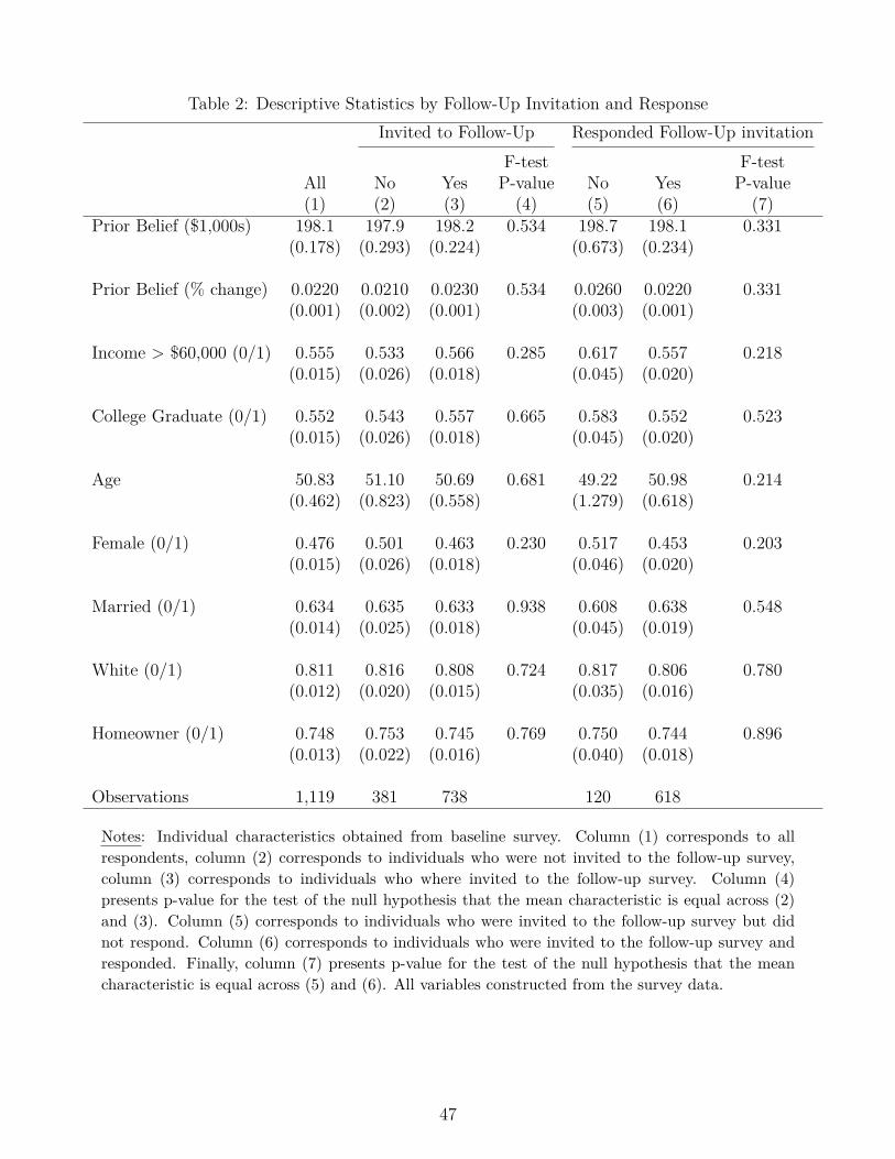
Table 2: Descriptive Statistics by Follow-Up Invitation and ResponseInvited to Follow-Up Responded Follow-Up invitation

F-test F-testAll No Yes P-value No Yes P-value(1) (2) (3) (4) (5) (6) (7)

Prior Belief ($1,000s) 198.1 197.9 198.2 0.534 198.7 198.1 0.331(0.178) (0.293) (0.224) (0.673) (0.234)

Prior Belief (% change) 0.0220 0.0210 0.0230 0.534 0.0260 0.0220 0.331(0.001) (0.002) (0.001) (0.003) (0.001)

Income > $60,000 (0/1) 0.555 0.533 0.566 0.285 0.617 0.557 0.218(0.015) (0.026) (0.018) (0.045) (0.020)

College Graduate (0/1) 0.552 0.543 0.557 0.665 0.583 0.552 0.523(0.015) (0.026) (0.018) (0.045) (0.020)

Age 50.83 51.10 50.69 0.681 49.22 50.98 0.214(0.462) (0.823) (0.558) (1.279) (0.618)

Female (0/1) 0.476 0.501 0.463 0.230 0.517 0.453 0.203(0.015) (0.026) (0.018) (0.046) (0.020)

Married (0/1) 0.634 0.635 0.633 0.938 0.608 0.638 0.548(0.014) (0.025) (0.018) (0.045) (0.019)

White (0/1) 0.811 0.816 0.808 0.724 0.817 0.806 0.780(0.012) (0.020) (0.015) (0.035) (0.016)

Homeowner (0/1) 0.748 0.753 0.745 0.769 0.750 0.744 0.896(0.013) (0.022) (0.016) (0.040) (0.018)

Observations 1,119 381 738 120 618

Notes: Individual characteristics obtained from baseline survey. Column (1) corresponds to allrespondents, column (2) corresponds to individuals who were not invited to the follow-up survey,column (3) corresponds to individuals who where invited to the follow-up survey. Column (4)presents p-value for the test of the null hypothesis that the mean characteristic is equal across (2)and (3). Column (5) corresponds to individuals who were invited to the follow-up survey but didnot respond. Column (6) corresponds to individuals who were invited to the follow-up survey andresponded. Finally, column (7) presents p-value for the test of the null hypothesis that the meancharacteristic is equal across (5) and (6). All variables constructed from the survey data.

47

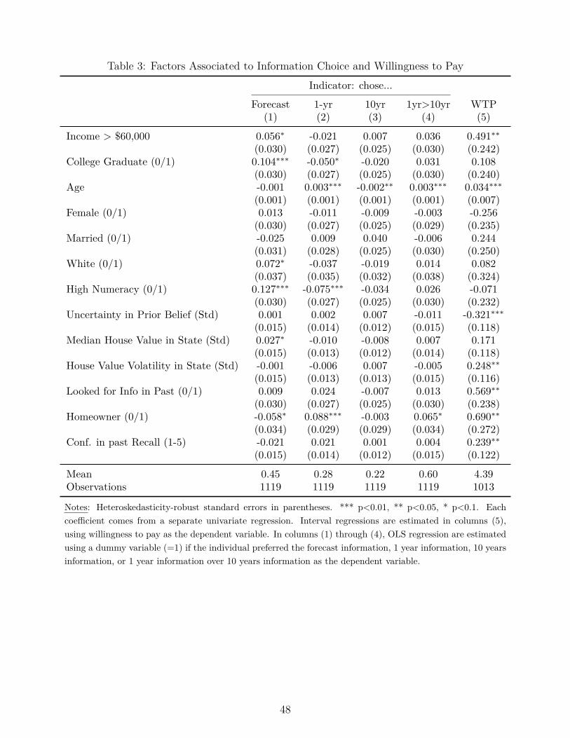
Table 3: Factors Associated to Information Choice and Willingness to PayIndicator: chose...

Forecast 1-yr 10yr 1yr>10yr WTP(1) (2) (3) (4) (5)

Income > $60,000 0.056∗ -0.021 0.007 0.036 0.491∗∗

(0.030) (0.027) (0.025) (0.030) (0.242)College Graduate (0/1) 0.104∗∗∗ -0.050∗ -0.020 0.031 0.108

(0.030) (0.027) (0.025) (0.030) (0.240)Age -0.001 0.003∗∗∗ -0.002∗∗ 0.003∗∗∗ 0.034∗∗∗

(0.001) (0.001) (0.001) (0.001) (0.007)Female (0/1) 0.013 -0.011 -0.009 -0.003 -0.256

(0.030) (0.027) (0.025) (0.029) (0.235)Married (0/1) -0.025 0.009 0.040 -0.006 0.244

(0.031) (0.028) (0.025) (0.030) (0.250)White (0/1) 0.072∗ -0.037 -0.019 0.014 0.082

(0.037) (0.035) (0.032) (0.038) (0.324)High Numeracy (0/1) 0.127∗∗∗ -0.075∗∗∗ -0.034 0.026 -0.071

(0.030) (0.027) (0.025) (0.030) (0.232)Uncertainty in Prior Belief (Std) 0.001 0.002 0.007 -0.011 -0.321∗∗∗

(0.015) (0.014) (0.012) (0.015) (0.118)Median House Value in State (Std) 0.027∗ -0.010 -0.008 0.007 0.171

(0.015) (0.013) (0.012) (0.014) (0.118)House Value Volatility in State (Std) -0.001 -0.006 0.007 -0.005 0.248∗∗

(0.015) (0.013) (0.013) (0.015) (0.116)Looked for Info in Past (0/1) 0.009 0.024 -0.007 0.013 0.569∗∗

(0.030) (0.027) (0.025) (0.030) (0.238)Homeowner (0/1) -0.058∗ 0.088∗∗∗ -0.003 0.065∗ 0.690∗∗

(0.034) (0.029) (0.029) (0.034) (0.272)Conf. in past Recall (1-5) -0.021 0.021 0.001 0.004 0.239∗∗

(0.015) (0.014) (0.012) (0.015) (0.122)

Mean 0.45 0.28 0.22 0.60 4.39Observations 1119 1119 1119 1119 1013

Notes: Heteroskedasticity-robust standard errors in parentheses. *** p<0.01, ** p<0.05, * p<0.1. Eachcoefficient comes from a separate univariate regression. Interval regressions are estimated in columns (5),using willingness to pay as the dependent variable. In columns (1) through (4), OLS regression are estimatedusing a dummy variable (=1) if the individual preferred the forecast information, 1 year information, 10 yearsinformation, or 1 year information over 10 years information as the dependent variable.

48

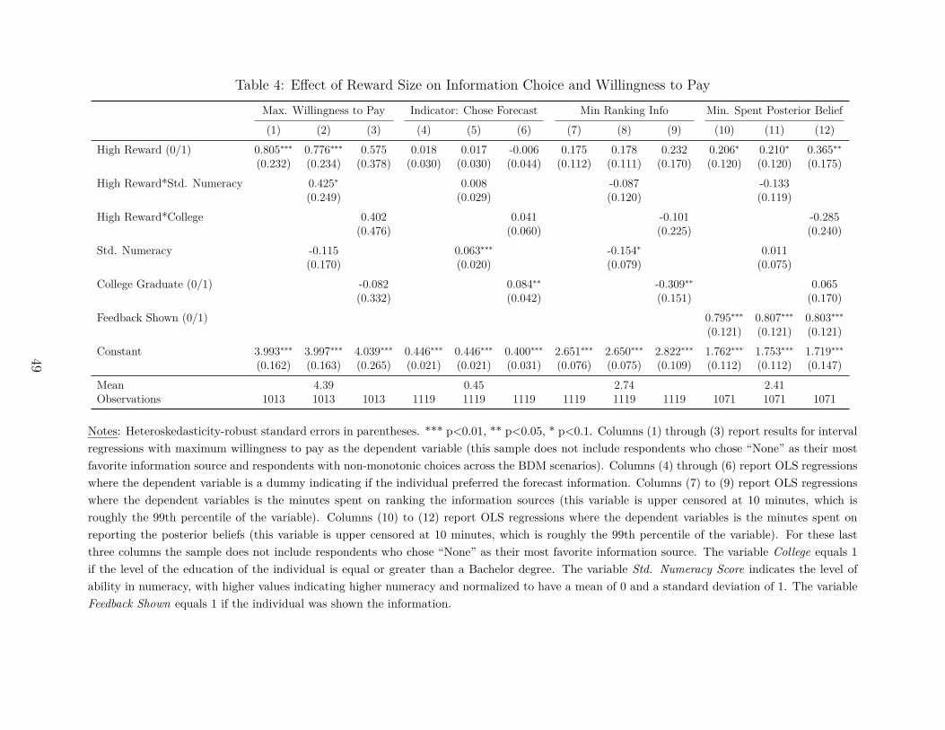
Table 4: Effect of Reward Size on Information Choice and Willingness to PayMax. Willingness to Pay Indicator: Chose Forecast Min Ranking Info Min. Spent Posterior Belief(1) (2) (3) (4) (5) (6) (7) (8) (9) (10) (11) (12)

High Reward (0/1) 0.805∗∗∗ 0.776∗∗∗ 0.575 0.018 0.017 -0.006 0.175 0.178 0.232 0.206∗ 0.210∗ 0.365∗∗(0.232) (0.234) (0.378) (0.030) (0.030) (0.044) (0.112) (0.111) (0.170) (0.120) (0.120) (0.175)

High Reward*Std. Numeracy 0.425∗ 0.008 -0.087 -0.133(0.249) (0.029) (0.120) (0.119)

High Reward*College 0.402 0.041 -0.101 -0.285(0.476) (0.060) (0.225) (0.240)

Std. Numeracy -0.115 0.063∗∗∗ -0.154∗ 0.011(0.170) (0.020) (0.079) (0.075)

College Graduate (0/1) -0.082 0.084∗∗ -0.309∗∗ 0.065(0.332) (0.042) (0.151) (0.170)

Feedback Shown (0/1) 0.795∗∗∗ 0.807∗∗∗ 0.803∗∗∗(0.121) (0.121) (0.121)

Constant 3.993∗∗∗ 3.997∗∗∗ 4.039∗∗∗ 0.446∗∗∗ 0.446∗∗∗ 0.400∗∗∗ 2.651∗∗∗ 2.650∗∗∗ 2.822∗∗∗ 1.762∗∗∗ 1.753∗∗∗ 1.719∗∗∗(0.162) (0.163) (0.265) (0.021) (0.021) (0.031) (0.076) (0.075) (0.109) (0.112) (0.112) (0.147)

Mean 4.39 0.45 2.74 2.41Observations 1013 1013 1013 1119 1119 1119 1119 1119 1119 1071 1071 1071

Notes: Heteroskedasticity-robust standard errors in parentheses. *** p<0.01, ** p<0.05, * p<0.1. Columns (1) through (3) report results for intervalregressions with maximum willingness to pay as the dependent variable (this sample does not include respondents who chose “None” as their mostfavorite information source and respondents with non-monotonic choices across the BDM scenarios). Columns (4) through (6) report OLS regressionswhere the dependent variable is a dummy indicating if the individual preferred the forecast information. Columns (7) to (9) report OLS regressionswhere the dependent variables is the minutes spent on ranking the information sources (this variable is upper censored at 10 minutes, which isroughly the 99th percentile of the variable). Columns (10) to (12) report OLS regressions where the dependent variables is the minutes spent onreporting the posterior beliefs (this variable is upper censored at 10 minutes, which is roughly the 99th percentile of the variable). For these lastthree columns the sample does not include respondents who chose “None” as their most favorite information source. The variable College equals 1if the level of the education of the individual is equal or greater than a Bachelor degree. The variable Std. Numeracy Score indicates the level ofability in numeracy, with higher values indicating higher numeracy and normalized to have a mean of 0 and a standard deviation of 1. The variableFeedback Shown equals 1 if the individual was shown the information.

49

Table 5: Cost of Information and Dispersion of ExpectationsLow Price High Price P-value Diff

(1) (2) (3)

Obtained Signal (%) 86.19 (1.057) 65.41 (1.545) 0.00

Expectations:

Prior Mean 2.15 (0.133) 2.22 (0.137) 0.74MAD 2.06 (0.098) 2.04 (0.100) 0.88Uncertainty 3.94 (0.124) 3.81 (0.130) 0.61Disagreement (%) 9.66 (0.92) 10.49 (1.00) 0.54

Posterior Mean 3.24 (0.141) 3.02 (0.143) 0.26MAD 2.21 (0.104) 2.13 (0.104) 0.59Uncertainty 2.87 (0.109) 2.96 (0.117) 0.68Disagreement (%) 19.03 (1.29) 19.51 (1.40) 0.80

Observations 536 477

Notes: This sample does not include respondents who chose “None” as their most favorite information sourceand respondents with non-monotonic choices across the BDM scenarios. The group Low-Price corresponds toindividuals randomly assigned to scenarios 1-4 (corresponding to prices from $0.01 to$1.5), while the groupHigh-Price corresponds to individuals randomly assigned to scenarios 5-11 (corresponding to prices from $2to $5). The average level, the dispersion (measured as mean absolute deviation, MAD), the uncertainty,and the fraction of disagreements within group is presented for the prior and posterior belief. The priorbelief refers to the expected change for home prices to the end of the year before the information, thatmay help with forecasting, was presented to individuals. Posterior belief refers to the expected change afterthe information was shown to individuals. Both in the prior and posterior belief the survey elicited therespondent’s subjective belief distribution about home prices. To measure uncertainty at the individual level,we fit these binned responses to a normal distribution for each individual, and use the estimated standarddeviation of the fitted distribution as a measure of individual-level uncertainty, with higher values denotinghigher uncertainty. A disagreement is defined as non-overlap of two respondents’ constructed 95% confidenceinterval; the table reports the fraction of all pairwise meetings that would result in a disagreement so defined.Columns (1) and (2) present the information for individuals who were randomly assigned to the Low and HighPrice respectively. Column (3) presents p-value for the test of the null hypothesis that the mean characteristicis equal across (1) and (2). Numbers in parentheses in each cell are standard errors.

50

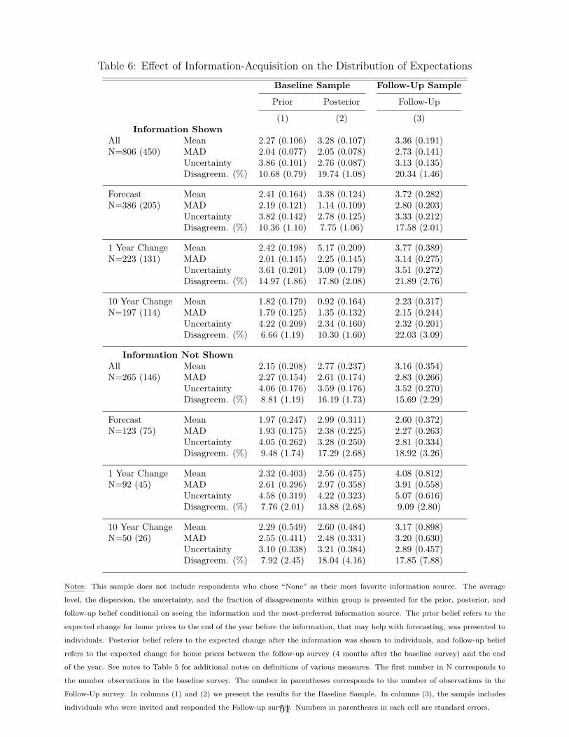
Table 6: Effect of Information-Acquisition on the Distribution of ExpectationsBaseline Sample Follow-Up Sample

Prior Posterior Follow-Up

(1) (2) (3)Information Shown

All Mean 2.27 (0.106) 3.28 (0.107) 3.36 (0.191)N=806 (450) MAD 2.04 (0.077) 2.05 (0.078) 2.73 (0.141)

Uncertainty 3.86 (0.101) 2.76 (0.087) 3.13 (0.135)Disagreem. (%) 10.68 (0.79) 19.74 (1.08) 20.34 (1.46)

Forecast Mean 2.41 (0.164) 3.38 (0.124) 3.72 (0.282)N=386 (205) MAD 2.19 (0.121) 1.14 (0.109) 2.80 (0.203)

Uncertainty 3.82 (0.142) 2.78 (0.125) 3.33 (0.212)Disagreem. (%) 10.36 (1.10) 7.75 (1.06) 17.58 (2.01)

1 Year Change Mean 2.42 (0.198) 5.17 (0.209) 3.77 (0.389)N=223 (131) MAD 2.01 (0.145) 2.25 (0.145) 3.14 (0.275)

Uncertainty 3.61 (0.201) 3.09 (0.179) 3.51 (0.272)Disagreem. (%) 14.97 (1.86) 17.80 (2.08) 21.89 (2.76)

10 Year Change Mean 1.82 (0.179) 0.92 (0.164) 2.23 (0.317)N=197 (114) MAD 1.79 (0.125) 1.35 (0.132) 2.15 (0.244)

Uncertainty 4.22 (0.209) 2.34 (0.160) 2.32 (0.201)Disagreem. (%) 6.66 (1.19) 10.30 (1.60) 22.03 (3.09)

Information Not ShownAll Mean 2.15 (0.208) 2.77 (0.237) 3.16 (0.354)N=265 (146) MAD 2.27 (0.154) 2.61 (0.174) 2.83 (0.266)

Uncertainty 4.06 (0.176) 3.59 (0.176) 3.52 (0.270)Disagreem. (%) 8.81 (1.19) 16.19 (1.73) 15.69 (2.29)

Forecast Mean 1.97 (0.247) 2.99 (0.311) 2.60 (0.372)N=123 (75) MAD 1.93 (0.175) 2.38 (0.225) 2.27 (0.263)

Uncertainty 4.05 (0.262) 3.28 (0.250) 2.81 (0.334)Disagreem. (%) 9.48 (1.74) 17.29 (2.68) 18.92 (3.26)

1 Year Change Mean 2.32 (0.403) 2.56 (0.475) 4.08 (0.812)N=92 (45) MAD 2.61 (0.296) 2.97 (0.358) 3.91 (0.558)

Uncertainty 4.58 (0.319) 4.22 (0.323) 5.07 (0.616)Disagreem. (%) 7.76 (2.01) 13.88 (2.68) 9.09 (2.80)

10 Year Change Mean 2.29 (0.549) 2.60 (0.484) 3.17 (0.898)N=50 (26) MAD 2.55 (0.411) 2.48 (0.331) 3.20 (0.630)

Uncertainty 3.10 (0.338) 3.21 (0.384) 2.89 (0.457)Disagreem. (%) 7.92 (2.45) 18.04 (4.16) 17.85 (7.88)

Notes: This sample does not include respondents who chose “None” as their most favorite information source. The average

level, the dispersion, the uncertainty, and the fraction of disagreements within group is presented for the prior, posterior, and

follow-up belief conditional on seeing the information and the most-preferred information source. The prior belief refers to the

expected change for home prices to the end of the year before the information, that may help with forecasting, was presented to

individuals. Posterior belief refers to the expected change after the information was shown to individuals, and follow-up belief

refers to the expected change for home prices between the follow-up survey (4 months after the baseline survey) and the end

of the year. See notes to Table 5 for additional notes on definitions of various measures. The first number in N corresponds to

the number observations in the baseline survey. The number in parentheses corresponds to the number of observations in the

Follow-Up survey. In columns (1) and (2) we present the results for the Baseline Sample. In columns (3), the sample includes

individuals who were invited and responded the Follow-up survey. Numbers in parentheses in each cell are standard errors.51

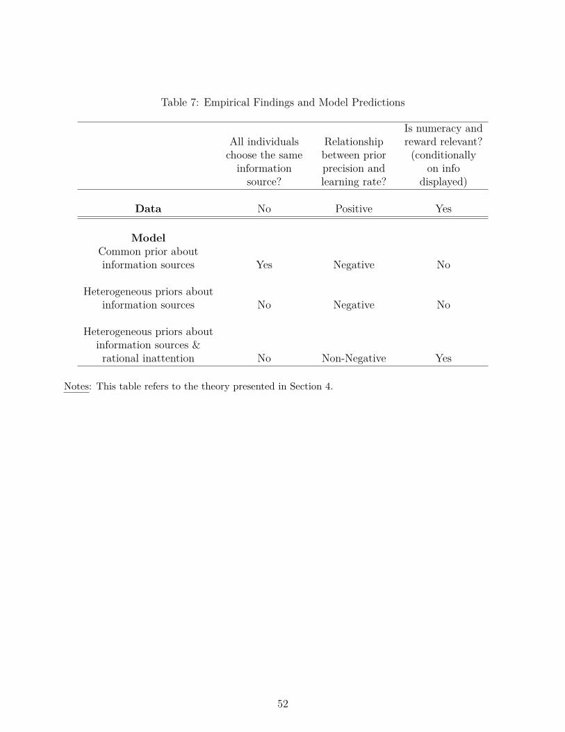
Table 7: Empirical Findings and Model Predictions

All individualschoose the sameinformationsource?

Relationshipbetween priorprecision andlearning rate?

Is numeracy andreward relevant?(conditionally

on infodisplayed)

Data No Positive Yes

ModelCommon prior aboutinformation sources Yes Negative No

Heterogeneous priors aboutinformation sources No Negative No

Heterogeneous priors aboutinformation sources &rational inattention No Non-Negative Yes

Notes: This table refers to the theory presented in Section 4.

52

Online Appendix: For Online Publication Only

A Additional Results

A.1 Decomposition of learning rates

In this section, we give more details about the identification of the learning rates. Figure A.3.ashows how the beliefs evolved after the information was provided. The y-axis indicates the revisionin national home price beliefs, i.e., posterior belief minus prior belief. The x-axis shows the “gap”between the signal and the prior belief. For instance, if the respondent had a prior belief of 1%and was shown the forecast of experts (which was 3.6% ), the x-axis would take the value of 2.6%.Intuitively, the x-axis shows how much potential for revision there is, and the y-axis shows theactual revision. If individuals fully reacted to the signal shown, we would expect all dots to lie onthe 45-degree line. If individuals did not react to the information, we would expect the dots to liein a horizontal line. The slope of the line is 0.561, which is not only highly statistically significant(p-value<0.001), but also economically substantial: it is closer to the case where individuals fullyreact to the information (slope of 1) than the case where individuals fully ignore the information(slope of 0).

Figure A.3.b is identical to Figure A.3.a, except that instead of corresponding to individuals whowere shown the signal, it corresponds to individuals who were not shown the signal. Consistentwith the typos and/or information search, there is reversion to the signal when the signal wasnot shown. However, the magnitude of this reversion to the signal is substantially lower than thecorresponding magnitude of the reversion when information is actually shown (0.163 versus 0.561).Figure 5.a presents the estimated learning rates (estimates of α), which roughly correspond to thedifference between the slopes in Figure A.3.a and A.3.b (i.e., the incremental convergence towardsthe signal due to the signal provision).

i

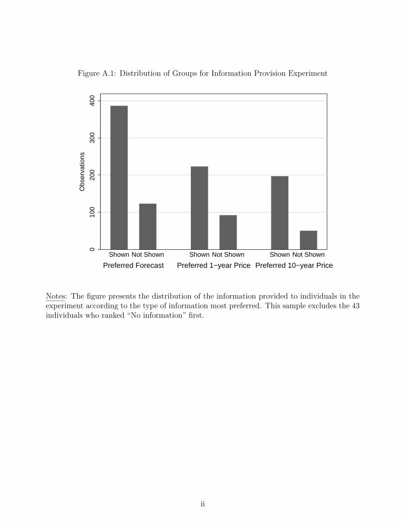
Figure A.1: Distribution of Groups for Information Provision Experiment

010

020

030

040

0

Obs

erva

tions

Preferred Forecast Preferred 1−year Price Preferred 10−year Price

Shown Not Shown Shown Not Shown Shown Not Shown

Notes: The figure presents the distribution of the information provided to individuals in theexperiment according to the type of information most preferred. This sample excludes the 43individuals who ranked “No information” first.

ii

Figure A.2: Certainty in Prior and Posterior Beliefs, By Information Provision

a. Prior Belief, No Info b. Prior Belief, Info

020

4060

Per

cent

X<90%

90%

<X<9

9%

99%

<X<1

01%

101%

<X<1

10%

X>110

%

X: Prior Belief

N = 265

020

4060

Per

cent

X<90%

90%

<X<9

9%

99%

<X<1

01%

101%

<X<1

10%

X>110

%

X: Prior Belief

N = 806

c. Posterior Belief, No Info d. Posterior Belief, Info

020

4060

Per

cent

X<90%

90%

<X<9

9%

99%

<X<1

01%

101%

<X<1

10%

X>110

%

X: Posterior Belief

N = 265

020

4060

Per

cent

X<90%

90%

<X<9

9%

99%

<X<1

01%

101%

<X<1

10%

X>110

%

X: Posterior Belief

N = 806

Notes: This sample does not include respondents who chose “None” as their most favoriteinformation source. Certainty in Prior and Posterior Beliefs according information provision.It measures how confident are individuals in their beliefs. The x-axis presents the range ofpossible variations in the estimation. And the y-axis presents the estimation of the percentchance of the possible variations.

iii

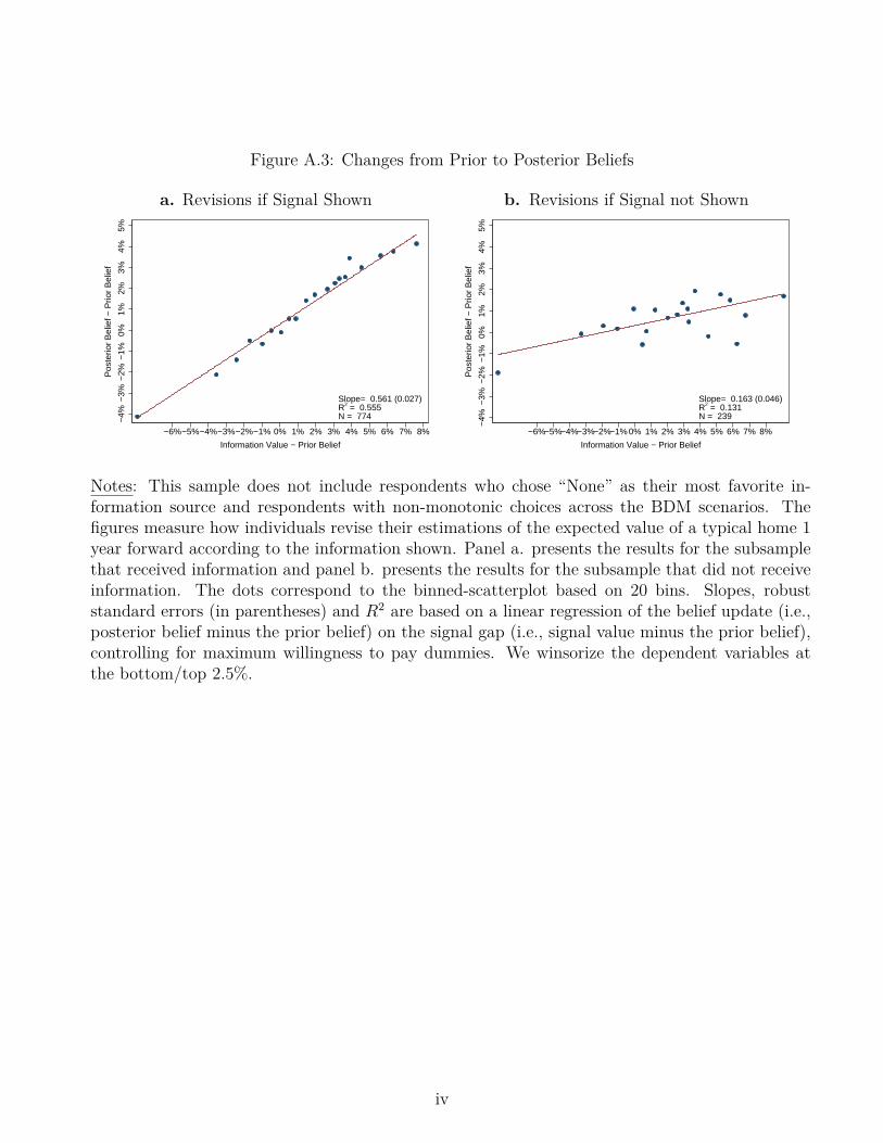
Figure A.3: Changes from Prior to Posterior Beliefs

a. Revisions if Signal Shown b. Revisions if Signal not Shown

−4%

−3%

−2%

−1%

0%1%

2%3%

4%5%

Pos

terio

r B

elie

f − P

rior

Bel

ief

−6%−5%−4%−3%−2%−1% 0% 1% 2% 3% 4% 5% 6% 7% 8%

Information Value − Prior Belief

Slope= 0.561 (0.027) R2 = 0.555 N = 774

−4%

−3%

−2%

−1%

0%1%

2%3%

4%5%

Pos

terio

r B

elie

f − P

rior

Bel

ief

−6%−5%−4%−3%−2%−1% 0% 1% 2% 3% 4% 5% 6% 7% 8%

Information Value − Prior Belief

Slope= 0.163 (0.046) R2 = 0.131 N = 239

Notes: This sample does not include respondents who chose “None” as their most favorite in-formation source and respondents with non-monotonic choices across the BDM scenarios. Thefigures measure how individuals revise their estimations of the expected value of a typical home 1year forward according to the information shown. Panel a. presents the results for the subsamplethat received information and panel b. presents the results for the subsample that did not receiveinformation. The dots correspond to the binned-scatterplot based on 20 bins. Slopes, robuststandard errors (in parentheses) and R2 are based on a linear regression of the belief update (i.e.,posterior belief minus the prior belief) on the signal gap (i.e., signal value minus the prior belief),controlling for maximum willingness to pay dummies. We winsorize the dependent variables atthe bottom/top 2.5%.

iv

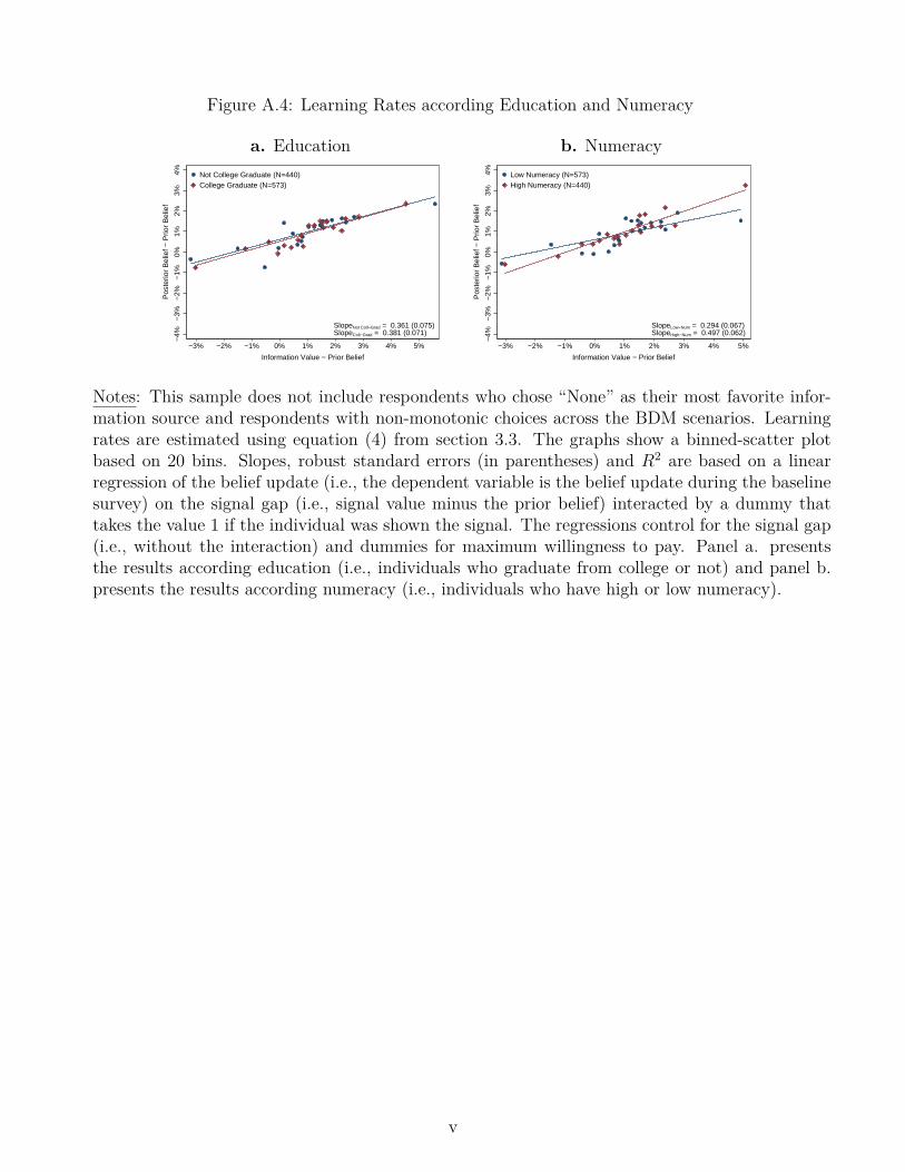
Figure A.4: Learning Rates according Education and Numeracy

a. Education b. Numeracy−

4%−

3%−

2%−

1%0%

1%2%

3%4%

Pos

terio

r B

elie

f − P

rior

Bel

ief

−3% −2% −1% 0% 1% 2% 3% 4% 5%

Information Value − Prior Belief

Not College Graduate (N=440)College Graduate (N=573)

SlopeNot Coll−Grad = 0.361 (0.075) SlopeColl−Grad = 0.381 (0.071)

−4%

−3%

−2%

−1%

0%1%

2%3%

4%

Pos

terio

r B

elie

f − P

rior

Bel

ief

−3% −2% −1% 0% 1% 2% 3% 4% 5%

Information Value − Prior Belief

Low Numeracy (N=573)High Numeracy (N=440)

SlopeLow−Num = 0.294 (0.067) SlopeHigh−Num = 0.497 (0.062)

Notes: This sample does not include respondents who chose “None” as their most favorite infor-mation source and respondents with non-monotonic choices across the BDM scenarios. Learningrates are estimated using equation (4) from section 3.3. The graphs show a binned-scatter plotbased on 20 bins. Slopes, robust standard errors (in parentheses) and R2 are based on a linearregression of the belief update (i.e., the dependent variable is the belief update during the baselinesurvey) on the signal gap (i.e., signal value minus the prior belief) interacted by a dummy thattakes the value 1 if the individual was shown the signal. The regressions control for the signal gap(i.e., without the interaction) and dummies for maximum willingness to pay. Panel a. presentsthe results according education (i.e., individuals who graduate from college or not) and panel b.presents the results according numeracy (i.e., individuals who have high or low numeracy).

v

Table A.1: Factors Associated to Information Choice and Willingness to Pay – Multivariate ResultsIndicator: chose...

Forecast 1-yr 10yr 1yr>10yr WTP(1) (2) (3) (4) (5)

Income > $60,000 0.040 -0.012 -0.004 0.041 0.496∗

(0.035) (0.032) (0.030) (0.035) (0.274)College Graduate (0/1) 0.067∗∗ -0.027 -0.017 0.028 0.053

(0.032) (0.029) (0.027) (0.032) (0.252)Age -0.000 0.002∗∗ -0.002∗∗∗ 0.003∗∗∗ 0.034∗∗∗

(0.001) (0.001) (0.001) (0.001) (0.008)Female (0/1) 0.036 -0.011 -0.021 0.025 0.019

(0.032) (0.028) (0.027) (0.032) (0.252)Married (0/1) -0.035 0.003 0.039 -0.023 -0.058

(0.036) (0.032) (0.029) (0.035) (0.278)White (0/1) 0.070∗ -0.044 -0.011 -0.008 -0.181

(0.039) (0.036) (0.034) (0.039) (0.332)High Numeracy (0/1) 0.110∗∗∗ -0.069∗∗ -0.038 0.019 -0.289

(0.032) (0.028) (0.027) (0.032) (0.243)Uncertainty in Prior Belief (Std) 0.006 0.004 0.005 -0.005 -0.257∗∗

(0.015) (0.014) (0.013) (0.015) (0.119)Median House Value in State (Std) 0.024 -0.006 -0.010 0.007 0.097

(0.015) (0.014) (0.013) (0.015) (0.125)House Value Volatility in State (Std) -0.009 -0.006 0.012 -0.009 0.195∗

(0.016) (0.014) (0.013) (0.016) (0.119)Looked for Info in Past (0/1) -0.008 0.033 -0.011 0.006 0.463∗

(0.031) (0.028) (0.026) (0.031) (0.249)Homeowner (0/1) -0.059 0.069∗∗ 0.014 0.027 0.125

(0.039) (0.032) (0.032) (0.039) (0.303)Conf. in past Recall (1-5) -0.012 0.011 0.001 -0.002 0.080

(0.015) (0.014) (0.013) (0.015) (0.128)

Mean 0.45 0.28 0.22 0.60 4.39Observations 1119 1119 1119 1119 1013

Notes: Heteroskedasticity-robust standard errors in parentheses. *** p<0.01, ** p<0.05, * p<0.1. Eachcolumn corresponds to a separate multivariate regression. An interval regression is estimated in columns(using willingness to pay as the dependent variable. In columns (1) through (4), OLS regressions are estimatedusing a dummy variable (=1) if the individual preferred the forecast information, 1 year information, 10 yearsinformation, or 1 year information over 10 years information as the dependent variable.

vi

B Supplementary Study

As a robustness check, we fielded a supplementary module one year later in the February 2018 SCEHousing Survey. The sample that takes this module has no overlap with the original study, sincerespondents are phased out of the SCE panel after 12 months. The main purpose of the module wasto investigate whether our result that the cross-sectional dispersion fails to go down in the groupthat is exogenously exposed to information (relative to the group that does not see information)is an artifact of the fact that respondents could not choose to buy multiple information sources.

In the supplementary survey, respondents were randomized into seeing no, one, or two piecesof information. Snapshots of this survey can be found in Appendix E. We next briefly summarizethe study design:

1. Stage 1- Prior Belief : This stage is identical to that in the main survey. Respondentsreport their year-end 2018 home price expectation as well as their subjective uncertainty.

2. Stage 2- Information Preferences: This stage is also quite similar to that in the mainsurvey. As in the main survey, respondents were randomized into a “High Reward” or “LowReward” group, and told that their home price expectation would be re-elicited. They werenext informed that they may have the opportunity to see some information before the re-elicitation. They were then asked: “If you had the choice of seeing one of the following twopieces of information, which one would you prefer to see?

(a) The change in the value of a typical home in the US over the last one year (2017).

(b) The change in the value of a typical home in the US over the last ten years (2008-2017).

(c) Neither of the above -- I would not like to see any information”

In addition, conditional on choosing option a (option b), they were also asked if they wouldlike to additionally see the information of option b (option a).

3. Stage 3- Posterior Belief: Depending on the stated preference for the information sourcein stage 2, respondents possibly saw additional information in this stage. Of those who saidthey preferred to see option a (that is, past one year home price change), a third were givenno information, a third were given information about home price change in the past year,and the remaining third were given information on both the past one and ten year changein home prices.41 For example, those who got to see both pieces of information were shown:

“We will next inform you about the change in the value of a typical home in the USover the last one year, and over the last ten years.

41Those who chose option b were similarly randomly allocated to a no-info group, a group that saw only thepast 10 year home price change, or a group that saw both changes. Those who chose option c did not see anyinformation.

vii

According to the Zillow Home Value Index, the value of a typical home in the USincreased by 6.5% over the last one year (December 2016 - December 2017) and by0.7% per year on average over the last ten years (December 2007 - December 2017).That means a typical home in the US that currently has a value of 206,300 dollarswould have had a value of 193,700 dollars in December 2016 and 191,700 dollarsin December 2007.

If home values were to increase at a pace of 6.5% next year (that is, last year’s pace),that would mean that the value of a typical home would be 219,710 dollars in December2018.

If home values were to increase at a pace of 0.7% next year (that is, the average annualpace over the last 10 years), that would mean that the value of a typical home would be207,744 dollars in December 2018.

Earlier in the survey, you reported that you thought the value of the typical home inthe US at the end of this year (in December 2018) would be 222,222 dollars. We wouldnow like to ask you again about the future value of a typical home in the US at theend of this year. What do you think the value of the typical home in the US will beat the end of this year (in December 2018)?”

Home price expectations were then re-elicited from everyone.At the very end of the survey, all respondents were asked whether they would have opted to

see the forecast of housing experts for year-end home prices instead of their preferred informationsource. In addition, respondents were asked to report their belief (on a 5-point scale) about (1)the ability of experts to forecast house price growth accurately, and (2) the credibility of expertsin general.

B.1 Empirical Analysis

A total of 1,144 respondents took the module. After applying the same sample selection criteria asin the main survey, we are left with 1,091 respondents. The sample is remarkably (and unsurpris-ingly) similar in observable characteristics to the main survey sample (shown in Table 1): 56.2%have household income of more than $60,000, 55.9% have a college degree or more, the mean ageis 51.0 years, 45.6% are female, 64.6% are married, 84.6% are white, and 75.3% are homeowners.We next discuss the main results.

B.1.1 Cross-Sectional Dispersion

Table B.1 describes the prior and posterior beliefs for the three groups: the group that saw bothpieces of information, the group that saw one piece of information, and the control group that saw

viii

no information. Recall that, conditional on one’s reported preference for information, assignmentto the three groups was random. Therefore, we can see how information – and more specificallybeing able to see multiple pieces of information – impacts the evolution of beliefs.

Information leads to a noticeable shift in mean beliefs, with the posterior belief significantlydifferent from the prior. However, beliefs shift even in the control group. Relative to the no-infogroup, the average posterior uncertainty declines quite a bit in the two groups that saw information,indicating that information led respondents to become more certain. However, dispersion – asmeasured by the mean absolute deviation of beliefs across individuals – does not decline for thegroups that saw information. In fact, the MAD goes up more for the information groups than forthe control group: the MAD increases by 0.15 percentage points for the control group and by 0.44(0.37) percentage points for the one- (two-) information group. We also see that our other measureof disagreement, based on whether a pair’s constructed confidence interval overlaps or not, alsoincreases a lot more for the information groups. For example, while a similar proportion of pairsdisagreed at the prior stage in the two-information group and the control group (13.5% and 13.1%,respectively), at the posterior stage, a substantially higher proportion of pairs disagreed in thetwo-information group (22.9% versus 16.1% in the control group). This corroborates the findingin the main survey that information does not lead to a convergence in beliefs. Here we see thatrandomly providing two signals at the same time has effects similar to providing just one signal.

B.1.2 Other results

Table B.2 shows some useful patterns in the data. Column (1) shows that 92 percent of therespondents, when presented with the choice of seeing information in Stage 2, opted for someinformation (opposed to choosing the “Neither” option). We see that higher-education respondentsand those with higher numeracy are significantly more likely to opt to see some information.

Conditional on wanting to see information, column (2) shows that 46 percent of the respondentspreferred the past one year home price change, with the remaining 54 percent preferring the pastten year home price change. Given the serial dependence in home price movements, as discussedin the paper, the past one year home price change is arguably a more useful resource. Column (3)shows that the vast majority of respondents – 85 percent – reported wanting to see both sourcesof information if that were an option. In both columns (2) and (3), we see a clear difference byeducation and numeracy along the lines that one would expect.

Finally column (4) validates the finding in the main experiment that lower-numeracy andless-educated respondents are significantly less likely to prefer the forecast of experts over thesealternative sources. Note, however, that here the vast majority – 68 percent – of respondentsreported that they would have preferred experts’ forecast over information about past home pricechanges, a substantially higher fraction than in the main experiment. This could be because thetwo studies differ in their specific setup.

ix

Experts’ forecast, as we discuss in the paper, should be the optimal information source. Todig deeper into why respondents may not choose the experts’ forecast, the module included twoquestions about the perceived ability of experts to give accurate forecasts, and their credibility.The last two columns of the table show statistics for these two variables. 49 percent of therespondents agreed or somewhat agreed (answered 4 or 5 on a 5-point scale) with the statement“Housing market experts can forecast future house price growth with high accuracy.” Likewise, 49percent of the respondents agreed or somewhat agreed with the statement “In general, I trust thecredibility of people referred to as experts.” The last column shows that lower-educated respondentsin fact have a lower level of trust in experts (44 percent of them trusting experts versus 53 percentof higher-educated respondents); they are also less likely to believe in the ability of experts toforecast accurately. In regression analysis (not presented here), we see that the 12 percentagepoint education gap in preferring experts (in column 4) declines by 2.5 points once we control forthe perceived ability and trust in experts. This suggests that at least some of the differences byeducation in preferring experts are driven by perceptions about experts’ credibility and ability.

x

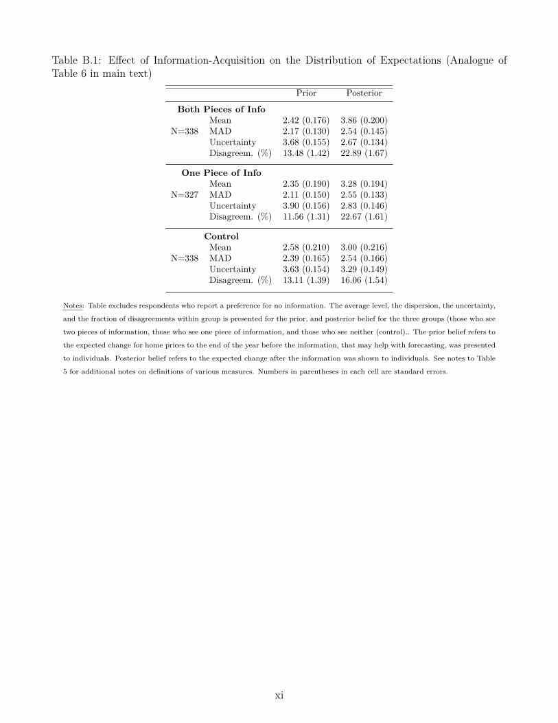
Table B.1: Effect of Information-Acquisition on the Distribution of Expectations (Analogue ofTable 6 in main text)

Prior Posterior

Both Pieces of InfoMean 2.42 (0.176) 3.86 (0.200)

N=338 MAD 2.17 (0.130) 2.54 (0.145)Uncertainty 3.68 (0.155) 2.67 (0.134)Disagreem. (%) 13.48 (1.42) 22.89 (1.67)

One Piece of InfoMean 2.35 (0.190) 3.28 (0.194)

N=327 MAD 2.11 (0.150) 2.55 (0.133)Uncertainty 3.90 (0.156) 2.83 (0.146)Disagreem. (%) 11.56 (1.31) 22.67 (1.61)

ControlMean 2.58 (0.210) 3.00 (0.216)

N=338 MAD 2.39 (0.165) 2.54 (0.166)Uncertainty 3.63 (0.154) 3.29 (0.149)Disagreem. (%) 13.11 (1.39) 16.06 (1.54)

Notes: Table excludes respondents who report a preference for no information. The average level, the dispersion, the uncertainty,

and the fraction of disagreements within group is presented for the prior, and posterior belief for the three groups (those who see

two pieces of information, those who see one piece of information, and those who see neither (control).. The prior belief refers to

the expected change for home prices to the end of the year before the information, that may help with forecasting, was presented

to individuals. Posterior belief refers to the expected change after the information was shown to individuals. See notes to Table

5 for additional notes on definitions of various measures. Numbers in parentheses in each cell are standard errors.

xi

Table B.2: Information Preferences and BeliefsInformation Preferences Perceptions

Obs Prefer AnyInfo

Prefer 1yr |Info

Prefer Both| Info

PreferExpert

FindExpertsAccurate

TrustExperts

(1) (2) (3) (4) (5) (6)

All 1091 0.92 0.46 0.85 0.68 0.49 0.49

High Reward 546 0.92 0.47 0.86 0.68 0.51 0.49Low Reward 545 0.92 0.45 0.85 0.67 0.47 0.49P-value 0.993 0.589 0.585 0.683 0.155 0.785

College Graduate 610 0.94 0.44 0.89 0.73 0.52 0.53Not College Grad 481 0.89 0.49 0.81 0.61 0.46 0.44P-value 0.001 0.128 0.001 0.000 0.064 0.005

High Numeracy 469 0.96 0.50 0.87 0.71 0.48 0.48Low Numeracy 622 0.89 0.43 0.84 0.65 0.51 0.50P-value 0.000 0.017 0.140 0.023 0.312 0.393

Notes: High reward corresponds to 100 dollar prize. High numeracy corresponds to no incorrect answers. Column variable definitionsare as follows: Prefer Any Info: Equals one if the respondent selected either 1 or 10 year info (opposed to no info); Prefer 1 year | Info:Conditional on selecting an information source, indicator that equals 1 if the respondent selected past 1 year info (those who selectedno info are dropped here); Prefer Both Info: Indicator that equals 1 is respondent reported she would like to see both pieces of info(those who selected no info are dropped); Prefer Expert: Indicator that equals 1 if respondent reports that she would have chosen expertforecast, if it had been a choice; Find Experts Accurate: Indicator for reporting a belief of expert accuracy of 4 or 5 on a 5-point scale;Trust Experts: Indicator for reporting a belief of expert credibility of 4 or 5 on a 5-point scale.

xii

C Model with a common prior over precisions

In the model in the paper, individual i has the prior belief that the precision of information sourcej ∈ 1, 2, 3 equals τj (i) ≡

(1/σ2

ε,j (i)). That τj is a function of i means that the prior belief about

the precision of information source j may differ across individuals. In the model in this appendix,all individuals instead share the same prior belief about the precision of the information sources.Cross-sectional heterogeneity in beliefs over precisions arises ex post.

Common prior over precisions. Individuals have the prior belief that each informationsource j is a noisy signal about the fundamental

xj = θ + εj,

where xj is the displayed information, θ and εj are mutually independent, and the noise εj isnormally distributed with mean zero. Individuals have the prior belief that one information sourcehas high precision, τH , and two information sources have low precision, τL, with τH > τL.42 Thethree information sources are homogenous a priori, that is, for any information source j ∈ 1, 2, 3,individuals assign probability 1/3 to information source j being the one with the high precision.

Processing information and posterior over precisions. The state of nature is the identityof the information source with high precision. Let j∗ ∈ 1, 2, 3 denote this information source.Individuals have imperfect information about the state of nature. As explained before, individualshave a uniform prior over j∗. Before selecting an information source, individuals can processinformation. Processing information is costly and processing more information is more costly.Processing information is modeled as receiving a noisy signal on the state. The signal announcesthe information source with the high precision and is correct with probability λ ∈ [1/3, 1], whereλ = 1/3 is a completely uninformative signal and λ = 1 is a perfectly informative signal. Ifthe signal is incorrect, it announces one of the two suboptimal information sources with equalprobability. Let z (i) ∈ 1, 2, 3 denote the signal received by individual i. For any two individualsi and i′, the signals z (i) and z (i′) are conditionally independent given j∗, which captures the ideathat information-processing mistakes arise on the level of the individual. It follows from Bayes’rule that for any individual i posterior beliefs are given by

Pr (j = j∗|z (i) = j) =λ1

3λ1

3 + (1− λ) 12

13 + (1− λ) 1

213

= λ,

andPr (j = j∗|z (i) 6= j) =

(1− λ) 13

(1− λ) 13 +

[λ+ (1− λ) 1

2

]13 +

[λ+ (1− λ) 1

2

]13

= 1− λ2 .

Processing more information amounts to a higher λ. The precise cost function for processing

42The assumption that two information sources have the same low precision is only for ease of exposition.

xiii

information will be specified below and will have the property that signals with a higher λ aremore costly.

First Action: Selecting an information source: The optimal choice of the informationsource given the realization of the signal on precisions is to follow the recommendation of thesignal. That is, the optimal action is to select information source j if and only if z (i) = j forany λ > (1/3) (“informative signal”). Intuitively, individuals have a uniform prior over j∗ and thesignal on the state is informative. Formally, λ > (1/3) ⇔ λ > 1−λ

2 . This has three implications.First, since there is idiosyncratic noise in the signal, individuals arrive at heterogeneous posteriorsover precisions and take heterogeneous actions, even though individuals have a common prior overprecisions. Second, for any sufficiently large group of individuals choosing to process information(i.e., for any sufficiently large group of individuals choosing λ > (1/3)), the information sourcewith the high precision will be the modal choice with a high probability. Third, once λ becomes achoice variable (see the paragraph on rational inattention below) the probability of selecting thehigh-precision information source will depend on household characteristics.

Conditional expectation of the fundamental: After selecting an information source andacquiring the information (more on that below), the information is displayed. Paying attention tothe displayed information is modeled as receiving a noisy signal on the displayed information

s(i) = xj + ψ (i) = θ + εj + ψ (i) ,

where j is the selected information source, xj is the displayed information, and ψ (i) is noise thatarises due to limited attention to the displayed information. The noise ψ (i) is assumed to benormally distributed with mean zero and variance σ2

ψ (i). Paying more attention to the displayedinformation is formalized as a smaller σ2

ψ (i). For the moment, we assume that this variance of noiseis exogenous. For example, one could set σ2

ψ (i) = 0 (“perfect attention to displayed information”).In an extension, we will solve the case where this variance of noise is endogenous, as in Section 4of the paper. Individuals assign probability λ to having acquired the right information source andprobability 1− λ to having acquired a wrong information source. The conditional expectation ofthe fundamental thus equals

E [θ|s (i) , z (i)] = λE [θ|s (i) , τj = τH ] + (1− λ)E [θ|s (i) , τj = τL]

= λ [µθ (i) +K (i, τH) (s(i)− µθ (i))] + (1− λ) [µθ (i) +K (i, τL) (s(i)− µθ (i))] ,

withK (i, τH) ≡ σ2

θ (i)σ2θ (i) + 1

τH+ σ2

ψ (i) and K (i, τL) ≡ σ2θ (i)

σ2θ (i) + 1

τL+ σ2

ψ (i) .

The second line follows from the fact that the fundamental and the signal s (i) have a multivariatenormal distribution for a given precision of the information source. The equation for the conditional

xiv

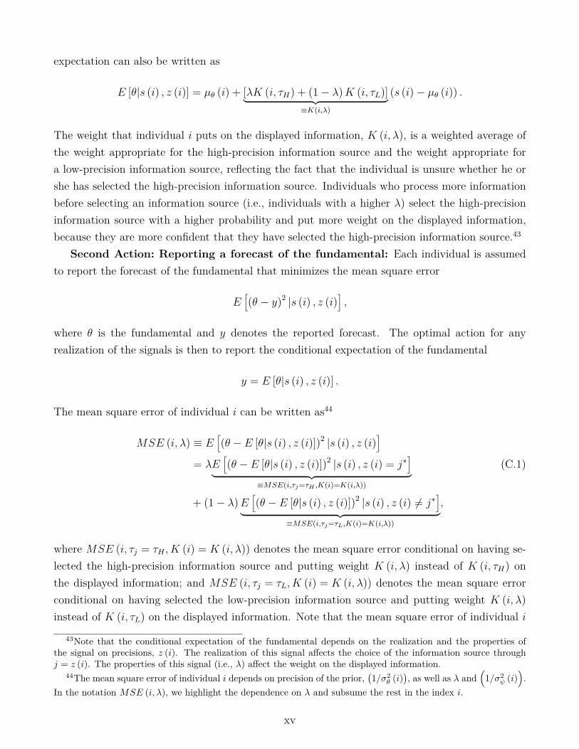
expectation can also be written as

E [θ|s (i) , z (i)] = µθ (i) + [λK (i, τH) + (1− λ)K (i, τL)]︸ ︷︷ ︸≡K(i,λ)

(s (i)− µθ (i)) .

The weight that individual i puts on the displayed information, K (i, λ), is a weighted average ofthe weight appropriate for the high-precision information source and the weight appropriate fora low-precision information source, reflecting the fact that the individual is unsure whether he orshe has selected the high-precision information source. Individuals who process more informationbefore selecting an information source (i.e., individuals with a higher λ) select the high-precisioninformation source with a higher probability and put more weight on the displayed information,because they are more confident that they have selected the high-precision information source.43

Second Action: Reporting a forecast of the fundamental: Each individual is assumedto report the forecast of the fundamental that minimizes the mean square error

E[(θ − y)2 |s (i) , z (i)

],

where θ is the fundamental and y denotes the reported forecast. The optimal action for anyrealization of the signals is then to report the conditional expectation of the fundamental

y = E [θ|s (i) , z (i)] .

The mean square error of individual i can be written as44

MSE (i, λ) ≡ E[(θ − E [θ|s (i) , z (i)])2 |s (i) , z (i)

]= λE

[(θ − E [θ|s (i) , z (i)])2 |s (i) , z (i) = j∗

]︸ ︷︷ ︸

≡MSE(i,τj=τH ,K(i)=K(i,λ))

(C.1)

+ (1− λ)E[(θ − E [θ|s (i) , z (i)])2 |s (i) , z (i) 6= j∗

]︸ ︷︷ ︸

≡MSE(i,τj=τL,K(i)=K(i,λ))

,

where MSE (i, τj = τH , K (i) = K (i, λ)) denotes the mean square error conditional on having se-lected the high-precision information source and putting weight K (i, λ) instead of K (i, τH) onthe displayed information; and MSE (i, τj = τL, K (i) = K (i, λ)) denotes the mean square errorconditional on having selected the low-precision information source and putting weight K (i, λ)instead of K (i, τL) on the displayed information. Note that the mean square error of individual i

43Note that the conditional expectation of the fundamental depends on the realization and the properties ofthe signal on precisions, z (i). The realization of this signal affects the choice of the information source throughj = z (i). The properties of this signal (i.e., λ) affect the weight on the displayed information.

44The mean square error of individual i depends on precision of the prior,(1/σ2

θ (i)), as well as λ and

(1/σ2

ψ (i)).

In the notation MSE (i, λ), we highlight the dependence on λ and subsume the rest in the index i.

xv

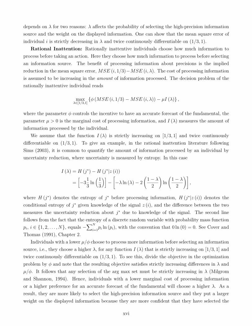
depends on λ for two reasons: λ affects the probability of selecting the high-precision informationsource and the weight on the displayed information. One can show that the mean square error ofindividual i is strictly decreasing in λ and twice continuously differentiable on (1/3, 1).

Rational Inattention: Rationally inattentive individuals choose how much information toprocess before taking an action. Here they choose how much information to process before selectingan information source. The benefit of processing information about precisions is the impliedreduction in the mean square error,MSE (i, 1/3)−MSE (i, λ). The cost of processing informationis assumed to be increasing in the amount of information processed. The decision problem of therationally inattentive individual reads

maxλ∈[1/3,1]

φ (MSE (i, 1/3)−MSE (i, λ))− µI (λ) ,

where the parameter φ controls the incentive to have an accurate forecast of the fundamental, theparameter µ > 0 is the marginal cost of processing information, and I (λ) measures the amount ofinformation processed by the individual.

We assume that the function I (λ) is strictly increasing on [1/3, 1] and twice continuouslydifferentiable on (1/3, 1). To give an example, in the rational inattention literature followingSims (2003), it is common to quantify the amount of information processed by an individual byuncertainty reduction, where uncertainty is measured by entropy. In this case

I (λ) = H (j∗)−H (j∗|z (i))

=[−31

3 ln(1

3

)]−[−λ ln (λ)− 2

(1− λ

2

)ln(

1− λ2

)],

where H (j∗) denotes the entropy of j∗ before processing information, H (j∗|z (i)) denotes theconditional entropy of j∗ given knowledge of the signal z (i), and the difference between the twomeasures the uncertainty reduction about j∗ due to knowledge of the signal. The second linefollows from the fact that the entropy of a discrete random variable with probability mass functionpi, i ∈ 1, 2, . . . , N, equals −

∑N

i=1pi ln (pi), with the convention that 0 ln (0) = 0. See Cover andThomas (1991), Chapter 2.

Individuals with a lower µ/φ choose to process more information before selecting an informationsource, i.e., they choose a higher λ, for any function I (λ) that is strictly increasing on [1/3, 1] andtwice continuously differentiable on (1/3, 1). To see this, divide the objective in the optimizationproblem by φ and note that the resulting objective satisfies strictly increasing differences in λ andµ/φ. It follows that any selection of the arg max set must be strictly increasing in λ (Milgromand Shannon, 1994). Hence, individuals with a lower marginal cost of processing informationor a higher preference for an accurate forecast of the fundamental will choose a higher λ. As aresult, they are more likely to select the high-precision information source and they put a largerweight on the displayed information because they are more confident that they have selected the

xvi

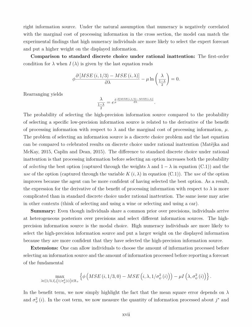
right information source. Under the natural assumption that numeracy is negatively correlatedwith the marginal cost of processing information in the cross section, the model can match theexperimental findings that high numeracy individuals are more likely to select the expert forecastand put a higher weight on the displayed information.

Comparison to standard discrete choice under rational inattention: The first-ordercondition for λ when I (λ) is given by the last equation reads

φ∂ [MSE (i, 1/3)−MSE (i, λ)]

∂λ− µ ln

(λ

1−λ2

)= 0.

Rearranging yieldsλ

1−λ2

= eφµ∂[MSE(i,1/3)−MSE(i,λ)]

∂λ .

The probability of selecting the high-precision information source compared to the probabilityof selecting a specific low-precision information source is related to the derivative of the benefitof processing information with respect to λ and the marginal cost of processing information, µ.The problem of selecting an information source is a discrete choice problem and the last equationcan be compared to celebrated results on discrete choice under rational inattention (Matějka andMcKay, 2015, Caplin and Dean, 2015). The difference to standard discrete choice under rationalinattention is that processing information before selecting an option increases both the probabilityof selecting the best option (captured through the weights λ and 1− λ in equation (C.1)) and theuse of the option (captured through the variable K (i, λ) in equation (C.1)). The use of the optionimproves because the agent can be more confident of having selected the best option. As a result,the expression for the derivative of the benefit of processing information with respect to λ is morecomplicated than in standard discrete choice under rational inattention. The same issue may arisein other contexts (think of selecting and using a wine or selecting and using a car).

Summary: Even though individuals share a common prior over precisions, individuals arriveat heterogeneous posteriors over precisions and select different information sources. The high-precision information source is the modal choice. High numeracy individuals are more likely toselect the high-precision information source and put a larger weight on the displayed informationbecause they are more confident that they have selected the high-precision information source.

Extensions: One can allow individuals to choose the amount of information processed beforeselecting an information source and the amount of information processed before reporting a forecastof the fundamental

maxλ∈[1/3,1],(1/σ2

ψ(i))∈R+

φ(MSE (i, 1/3, 0)−MSE

(i, λ, 1/σ2

ψ (i)))− µI

(λ, σ2

ψ (i)).

In the benefit term, we now simply highlight the fact that the mean square error depends on λ

and σ2ψ (i). In the cost term, we now measure the quantity of information processed about j∗ and

xvii

the quantity of information processed about the displayed information xj. The total quantity ofinformation processed depends on λ and σ2

ψ (i).One can also introduce the fixed cost of acquiring access to the information source. As pointed

out in Section 4 of the paper, the willingness to pay for access to the selected information sourceequals the benefit of access to the information source, φ

(MSE (i, 1/3, 0)−MSE

(i, λ, 1/σ2

ψ (i)))

,net of the cost of processing the displayed information at the optimal λ and σ2

ψ (i). The individualacquires access to the information source if this willingness to pay exceeds the cost.

xviii

D Survey Instrument: Main Study

We will next be asking you about your expectations of nationwide home price changes.

BACK NEXT

0% 25% 50% 75% 100%

© 2017 nielsen |

xix

As of December 2016, the value of the median or "typical" home in the US was 193,800dollars (according to Zillow.com). Now, think about how the value of the typical home inthe US has changed over time. (By value, we mean how much that typical home wouldapproximately sell for.)

What do you think the value of such a home was

Please provide your best guess in each box below.

one year earlier (in December 2015)? 193000 dollars

ten years earlier (in December 2006)? 190000 dollars

How confident are you in your answers?

Please select only one.

Not at allconfident

Somewhatconfident Very confident

1 2 3 4 5

BACK NEXT

0% 25% 50% 75% 100%

© 2017 nielsen |

xx

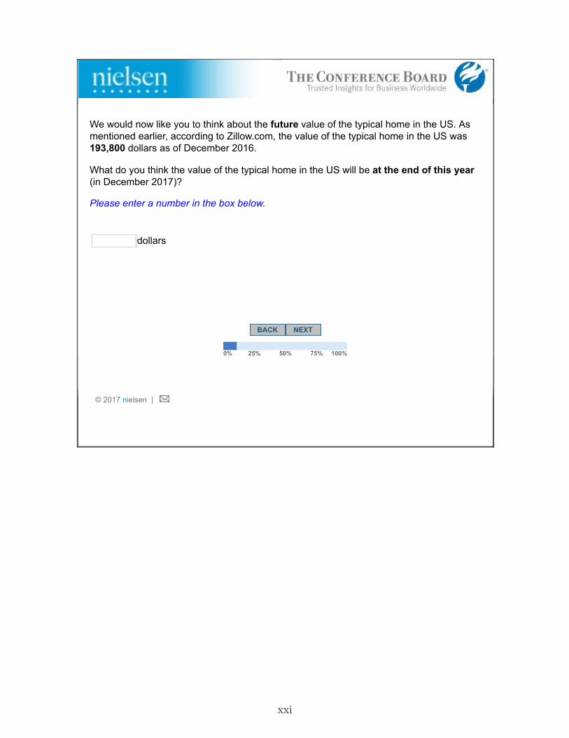
We would now like you to think about the future value of the typical home in the US. Asmentioned earlier, according to Zillow.com, the value of the typical home in the US was193,800 dollars as of December 2016.

What do you think the value of the typical home in the US will be at the end of this year(in December 2017)?

Please enter a number in the box below.

dollars

BACK NEXT

0% 25% 50% 75% 100%

© 2017 nielsen |

xxi

We would now like you to think about the future value of the typical home in the US. Asmentioned earlier, according to Zillow.com, the value of the typical home in the US was193,800 dollars as of December 2016.

What do you think the value of the typical home in the US will be at the end of this year(in December 2017)?

Please enter a number in the box below.

194000 dollars

You said that you expect the value of a typical home in the US to be $194,000 at the endof this year. That is, you expect home prices to change by 0.10% over the course of theyear 2017.

If not, please change your answer.

BACK NEXT

0% 25% 50% 75% 100%

© 2017 nielsen |

xxii

You estimated the value of the typical home in the US to be 194,000 dollars at the end ofthis year. Now we want to ask you about how confident you are about this forecast.

What do you think is the percent chance (or chances out of 100) that the value of such ahome at the end of this year (in December 2017) will be...

(Please note: The numbers need to add up to 100.)

Less than 174,600 dollars percent chance

Between 174,600 and 192,100 dollars percent chance

Between 192,100 and 195,900 dollars percent chance

Between 195,900 and 213,400 dollars percent chance

More than 213,400 dollars percent chance

TOTAL 0

BACK NEXT

0% 25% 50% 75% 100%

© 2017 nielsen |

xxiii

Earlier in the survey, we asked you to forecast the value of a typical home in the US at theend of this year. Later in this survey, we will ask you to do so again.

This time, we will reward the accuracy of your forecast: you will have a chance ofreceiving $100. There is roughly a 10% chance that you will be eligible to receive thisprize: we will select at random 60 out of about 600 people answering this question. Then,those respondents whose forecast is within 1% of the actual value of a typical US homeat the end of this year will receive $100.

Your payment will depend on your answer, so consider this question carefully. You will beinformed at the end of the survey if you have been chosen for this potential prize.

BACK NEXT

0% 25% 50% 75% 100%

© 2017 nielsen |

xxiv

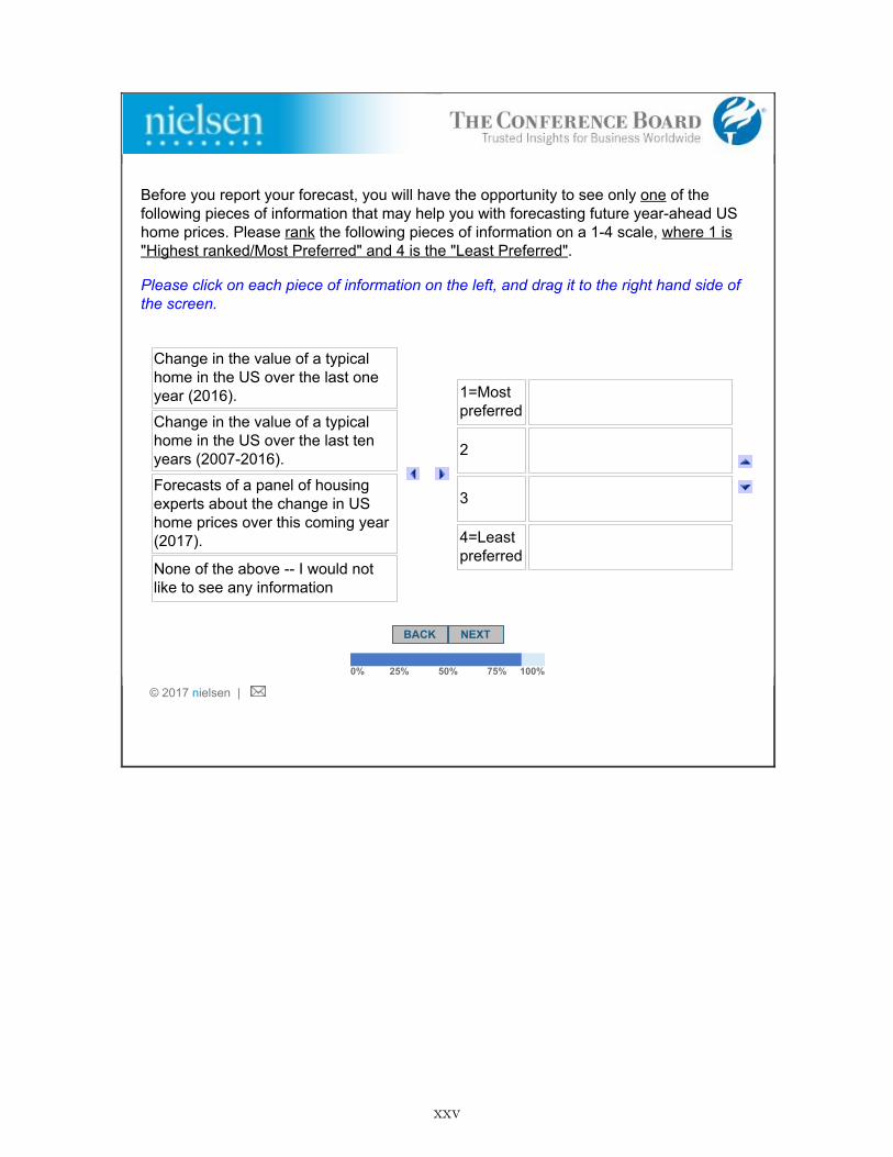
Before you report your forecast, you will have the opportunity to see only one of thefollowing pieces of information that may help you with forecasting future year­ahead UShome prices. Please rank the following pieces of information on a 1­4 scale, where 1 is"Highest ranked/Most Preferred" and 4 is the "Least Preferred".

Please click on each piece of information on the left, and drag it to the right hand side ofthe screen.

Change in the value of a typicalhome in the US over the last oneyear (2016).

Change in the value of a typicalhome in the US over the last tenyears (2007­2016).

Forecasts of a panel of housingexperts about the change in UShome prices over this coming year(2017).

None of the above ­­ I would notlike to see any information

1=Mostpreferred

2

3

4=Leastpreferred

BACK NEXT

0% 25% 50% 75% 100%

© 2017 nielsen |

xxv

You said that you would most prefer seeing information on the change in the value of atypical home in the US over the last one year (2016). Now we want to assess how muchyou would value this information.

You will next be presented with 11 scenarios. In each scenario, you will be given thechoice of either seeing information about the change in the value of a typical home in theUS over the last one year (2016) OR receiving extra money with the check that you willbe getting for completing this survey. The amount of money that you will be offered inthese scenarios is pre­determined, and goes from $0.01 to $5. For instance, in Scenario1, you will need to choose between seeing information or receiving $0.01; and inScenario 11, you will need to choose between seeing information or receiving $5.

We will draw one of these 11 scenarios at random for you. Your choice in the randomlychosen scenario will then be implemented. That is, you will have to make 11 choices, butonly one of those choices will be implemented.

Since one scenario will be picked at random, your choices will not affect which scenariowill be chosen.

BACK NEXT

0% 25% 50% 75% 100%

© 2017 nielsen |

xxvi

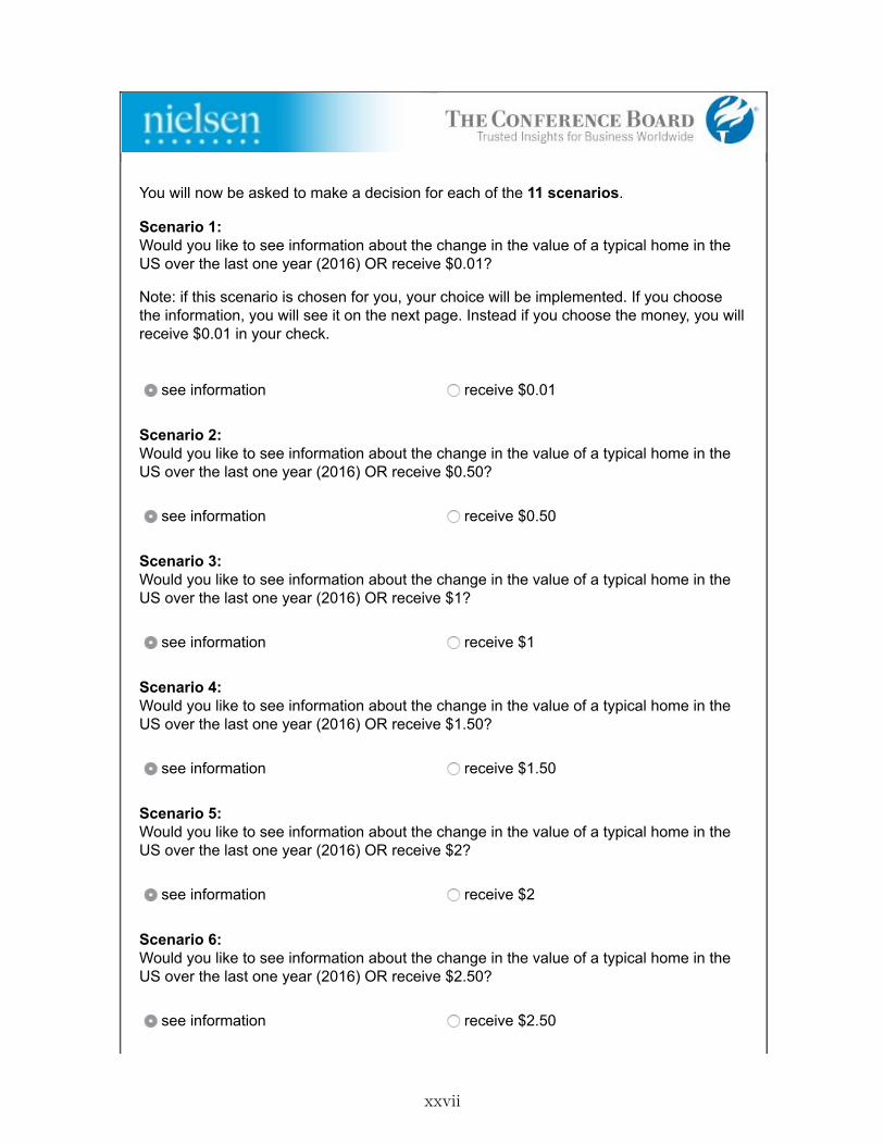
You will now be asked to make a decision for each of the 11 scenarios.

Scenario 1:Would you like to see information about the change in the value of a typical home in theUS over the last one year (2016) OR receive $0.01?

Note: if this scenario is chosen for you, your choice will be implemented. If you choosethe information, you will see it on the next page. Instead if you choose the money, you willreceive $0.01 in your check.

see information receive $0.01

Scenario 2:Would you like to see information about the change in the value of a typical home in theUS over the last one year (2016) OR receive $0.50?

see information receive $0.50

Scenario 3:Would you like to see information about the change in the value of a typical home in theUS over the last one year (2016) OR receive $1?

see information receive $1

Scenario 4:Would you like to see information about the change in the value of a typical home in theUS over the last one year (2016) OR receive $1.50?

see information receive $1.50

Scenario 5:Would you like to see information about the change in the value of a typical home in theUS over the last one year (2016) OR receive $2?

see information receive $2

Scenario 6:Would you like to see information about the change in the value of a typical home in theUS over the last one year (2016) OR receive $2.50?

see information receive $2.50

xxvii

Scenario 7:Would you like to see information about the change in the value of a typical home in theUS over the last one year (2016) OR receive $3?

see information receive $3

Scenario 8:Would you like to see information about the change in the value of a typical home in theUS over the last one year (2016) OR receive $3.50?

see information receive $3.50

Scenario 9:Would you like to see information about the change in the value of a typical home in theUS over the last one year (2016) OR receive $4?

see information receive $4

Scenario 10:Would you like to see information about the change in the value of a typical home in theUS over the last one year (2016) OR receive $4.50?

see information receive $4.50

Scenario 11:Would you like to see information about the change in the value of a typical home in theUS over the last one year (2016) OR receive $5?

see information receive $5

BACK NEXT

0% 25% 50% 75% 100%

© 2017 nielsen |

xxviii

We would now like to ask you again about the future value of a typical home in the US atthe end of this year.

Remember you will now have a chance of receiving $100 for the accuracy of yourforecast. There is roughly a 10% chance that you will be eligible to receive this prize.About 600 people are answering this question, of whom 60 will be randomly picked forthis potential prize.

If you are picked, you will receive $100 if your forecast is within 1 percent of the actualmedian home value in the US in December 2017 (according to the Zillow Home ValueIndex).

Your payment will depend on your answer, so consider this question carefully. You will beinformed at the end of the survey if you have been chosen for this potential prize.

NEXT

0% 25% 50% 75% 100%

© 2017 nielsen |

xxix

Scenario 1 was picked at random for you.

You had chosen to receive information about the change in the value of a typical home inthe US over the last one year (2016).

According to the Zillow Home Value Index, the value of a typical home in the USincreased by 6.8% over the last one year (December 2015 ­ December 2016 ). Thatmeans a typical home in the US that currently has a value of 193,800 dollars would havehad a value of 181,500 dollars in December 2015. If home values were to increase at apace of 6.8% next year, that would mean that the value of a typical home would be206,978 dollars in December 2017.

Earlier in the survey, you reported that you thought the value of the typical home in theUS at the end of this year (in December 2017) would be 194,000 dollars.

We would now like to ask you again about the future value of a typical home in the US atthe end of this year.

NEXT

0% 25% 50% 75% 100%

© 2017 nielsen |

xxx

According to the Zillow Home Value Index, the value of a typical home in the USincreased by 6.8% over the last one year (December 2015 ­ December 2016 ). Thatmeans a typical home in the US that currently has a value of 193,800 dollars would havehad a value of 181,500 dollars in December 2015. If home values were to increase at apace of 6.8% next year, that would mean that the value of a typical home would be206,978 dollars in December 2017.

Earlier in the survey, you reported that you thought the value of the typical home in theUS at the end of this year (in December 2017) would be 194,000 dollars.

We would now like to ask you again about the future value of a typical home in the US atthe end of this year.

What do you think the value of the typical home in the US will be at the end of this year(in December 2017)?

Please enter a number in the box below.

dollars

NEXT

0% 25% 50% 75% 100%

© 2017 nielsen |

xxxi

According to the Zillow Home Value Index, the value of a typical home in the USincreased by 6.8% over the last one year (December 2015 ­ December 2016 ). Thatmeans a typical home in the US that currently has a value of 193,800 dollars would havehad a value of 181,500 dollars in December 2015. If home values were to increase at apace of 6.8% next year, that would mean that the value of a typical home would be206,978 dollars in December 2017.

Earlier in the survey, you reported that you thought the value of the typical home in theUS at the end of this year (in December 2017) would be 194,000 dollars.

We would now like to ask you again about the future value of a typical home in the US atthe end of this year.

What do you think the value of the typical home in the US will be at the end of this year(in December 2017)?

Please enter a number in the box below.

200000 dollars

You said that you expect the value of a typical home in the US to be $200,000 at the endof this year. That is, you expect home prices to change by 3.20% over the course of theyear 2017.

If not, please change your answer.

NEXT

0% 25% 50% 75% 100%

© 2017 nielsen |

xxxii

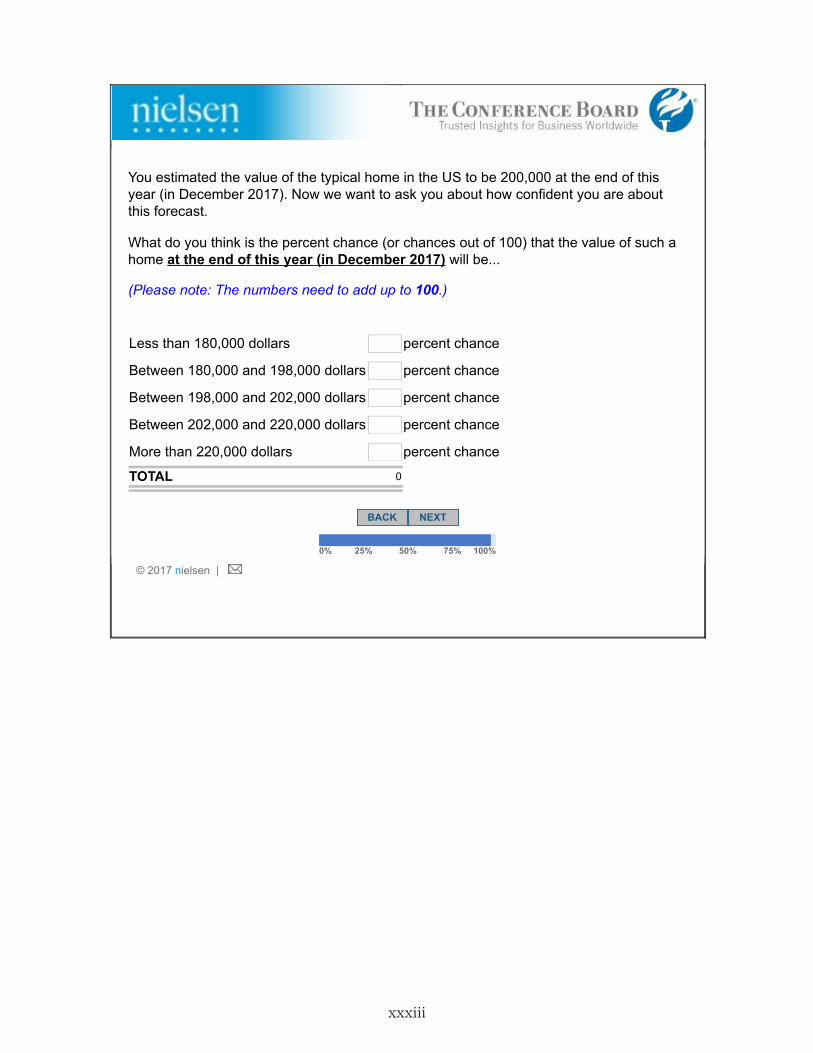
You estimated the value of the typical home in the US to be 200,000 at the end of thisyear (in December 2017). Now we want to ask you about how confident you are aboutthis forecast.

What do you think is the percent chance (or chances out of 100) that the value of such ahome at the end of this year (in December 2017) will be...

(Please note: The numbers need to add up to 100.)

Less than 180,000 dollars percent chance

Between 180,000 and 198,000 dollars percent chance

Between 198,000 and 202,000 dollars percent chance

Between 202,000 and 220,000 dollars percent chance

More than 220,000 dollars percent chance

TOTAL 0

BACK NEXT

0% 25% 50% 75% 100%

© 2017 nielsen |

xxxiii

It was ok to refer to other sources (such as Google, Zillow, etc.) when taking the survey.Did you use any such sources when answering any question in the survey?

Please select only one.

Yes

No

BACK NEXT

0% 25% 50% 75% 100%

© 2017 nielsen |

xxxiv

E Survey Instrument: Supplementary Study

We will next be asking you about your expectations of nationwide home price changes.

BACK NEXT

0% 25% 50% 75% 100%

© 2018 nielsen |

xxxv

As of December 2017, the value of the median or "typical" home in the US was 206,300dollars (according to Zillow.com). Now, think about how the value of the typical home in theUS has changed over time. (By value, we mean how much that typical home wouldapproximately sell for.)

What do you think the value of such a home was

Please provide your best guess in each box below.

one year earlier (in December 2016)? dollars

ten years earlier (in December 2006)? dollars

How confident are you in your answers?

Please select only one.

Not at allconfident

Somewhatconfident Very confident

1 2 3 4 5

BACK NEXT

0% 25% 50% 75% 100%

© 2018 nielsen |

xxxvi

We would now like you to think about the future value of the typical home in the US. Asmentioned earlier, according to Zillow.com, the value of the typical home in the US was206,300 dollars as of December 2017.

What do you think the value of the typical home in the US will be at the end of this year (inDecember 2018)?

Please enter a number in the box below.

dollars

You said that you expect the value of a typical home in the US to be $210,000 at the end ofthis year. That is, you expect home prices to change by 1.79% over the course of the year2018.

If not, please change your answer.

BACK NEXT

0% 25% 50% 75% 100%

© 2018 nielsen |

210000

xxxvii

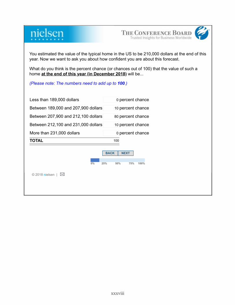
You estimated the value of the typical home in the US to be 210,000 dollars at the end of thisyear. Now we want to ask you about how confident you are about this forecast.

What do you think is the percent chance (or chances out of 100) that the value of such ahome at the end of this year (in December 2018) will be...

(Please note: The numbers need to add up to 100.)

Less than 189,000 dollars percent chance

Between 189,000 and 207,900 dollars percent chance

Between 207,900 and 212,100 dollars percent chance

Between 212,100 and 231,000 dollars percent chance

More than 231,000 dollars percent chance

TOTAL 100

BACK NEXT

0% 25% 50% 75% 100%

© 2018 nielsen |

0

10

80

10

0

xxxviii

Earlier in the survey, we asked you to forecast the value of a typical home in the US at theend of this year. Later in this survey, we will ask you to do so again.

This time, we will reward the accuracy of your forecast: you will have a chance of receiving$100. There is roughly a 10% chance that you will be eligible to receive this prize: we willselect at random 60 out of about 600 people answering this question. Then, thoserespondents whose forecast is within 1% of the actual value of a typical US home at the endof this year will receive $100.

Your payment will depend on your answer, so consider this question carefully. You will beinformed at the end of the survey if you have been chosen for this potential prize.

BACK NEXT

0% 25% 50% 75% 100%

© 2018 nielsen |

xxxix

Before you report your forecast, you will possibly have the opportunity to see someinformation that may help you with forecasting future year-ahead US home prices.

If you had the choice of seeing one of the following two pieces of information, which onewould you prefer to see?

I would prefer to see:

Please select only one.

The change in the value of a typical home in the US over the last one year (2017).

The change in the value of a typical home in the US over the last ten years (2008-2017).

Neither of the above -- I would not like to see any information

BACK NEXT

0% 25% 50% 75% 100%

© 2018 nielsen |

xl

You stated that your preferred information is about the change in home values over the lastone year. If possible, would you additionally want to see information about the change inhome values over the last ten years as well?

Please select only one.

Yes, I would like to see this additional information.

No, I would prefer not to see this additional information.

BACK NEXT

0% 25% 50% 75% 100%

© 2018 nielsen |

xli

We would now like to ask you again about the future value of a typical home in the US at theend of this year.

Remember you will now have a chance of receiving $100 for the accuracy of your forecast.There is roughly a 10% chance that you will be eligible to receive this prize. About 600people are answering this question, of whom 60 will be randomly picked for this potentialprize.

If you are picked, you will receive $100 if your forecast is within 1 percent of the actualmedian home value in the US in December 2018 (according to the Zillow Home ValueIndex).

Your payment will depend on your answer, so consider this question carefully. You will beinformed at the end of the survey if you have been chosen for this potential prize.

NEXT

0% 25% 50% 75% 100%

© 2018 nielsen |

xlii

We will next inform you about the change in the value of a typical home in the US over thelast one year.

According to the Zillow Home Value Index, the value of a typical home in the US increasedby 6.5% over the last one year (December 2016 - December 2017). That means a typicalhome in the US that currently has a value of 206,300 dollars would have had a value of193,700 dollars in December 2016. If home values were to increase at a pace of 6.5% nextyear, that would mean that the value of a typical home would be 219,710 dollars inDecember 2018.

Earlier in the survey, you reported that you thought the value of the typical home in the US atthe end of this year (in December 2018) would be 210,000 dollars.

We would now like to ask you again about the future value of a typical home in the US at theend of this year.

What do you think the value of the typical home in the US will be at the end of this year (inDecember 2018)?

Please enter a number in the box below.

dollars

Click here to view the official rules for the game.

You said that you expect the value of a typical home in the US to be $230,000 at the end ofthis year. That is, you expect home prices to change by 11.49% over the course of the year2018.

If not, please change your answer.

BACK NEXT

0% 25% 50% 75% 100%

© 2018 nielsen |

230000

xliii

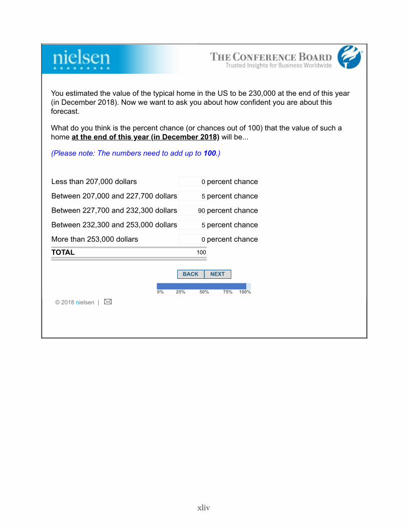
You estimated the value of the typical home in the US to be 230,000 at the end of this year(in December 2018). Now we want to ask you about how confident you are about thisforecast.

What do you think is the percent chance (or chances out of 100) that the value of such ahome at the end of this year (in December 2018) will be...

(Please note: The numbers need to add up to 100.)

Less than 207,000 dollars percent chance

Between 207,000 and 227,700 dollars percent chance

Between 227,700 and 232,300 dollars percent chance

Between 232,300 and 253,000 dollars percent chance

More than 253,000 dollars percent chance

TOTAL 100

BACK NEXT

0% 25% 50% 75% 100%

© 2018 nielsen |

0

5

90

5

0

xliv

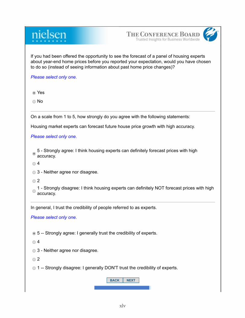
If you had been offered the opportunity to see the forecast of a panel of housing expertsabout year-end home prices before you reported your expectation, would you have chosento do so (instead of seeing information about past home price changes)?

Please select only one.

Yes

No

On a scale from 1 to 5, how strongly do you agree with the following statements:

Housing market experts can forecast future house price growth with high accuracy.

Please select only one.

5 - Strongly agree: I think housing experts can definitely forecast prices with highaccuracy.4

3 - Neither agree nor disagree.

21 - Strongly disagree: I think housing experts can definitely NOT forecast prices with highaccuracy.

In general, I trust the credibility of people referred to as experts.

Please select only one.

5 -- Strongly agree: I generally trust the credibility of experts.

4

3 - Neither agree nor disagree.

2

1 -- Strongly disagree: I generally DON'T trust the credibility of experts.

BACK NEXT

xlv