endogenous model

8/8/2019 Endogenous Model

http://slidepdf.com/reader/full/endogenous-model 1/24

Government Spending in a Simple Model of Endogeneous GrowthAuthor(s): Robert J. BarroSource: The Journal of Political Economy, Vol. 98, No. 5, Part 2: The Problem of Development:A Conference of the Institute for the Study of Free Enterprise Systems (Oct., 1990), pp.S103-S125Published by: The University of Chicago PressStable URL: http://www.jstor.org/stable/2937633

Accessed: 08/10/2010 04:17

Your use of the JSTOR archive indicates your acceptance of JSTOR's Terms and Conditions of Use, available athttp://www.jstor.org/page/info/about/policies/terms.jsp. JSTOR's Terms and Conditions of Use provides, in part, that unless

you have obtained prior permission, you may not download an entire issue of a journal or multiple copies of articles, and you

may use content in the JSTOR archive only for your personal, non-commercial use.

Please contact the publisher regarding any further use of this work. Publisher contact information may be obtained at

http://www.jstor.org/action/showPublisher?publisherCode=ucpress.

Each copy of any part of a JSTOR transmission must contain the same copyright notice that appears on the screen or printed

page of such transmission.

JSTOR is a not-for-profit service that helps scholars, researchers, and students discover, use, and build upon a wide range of

content in a trusted digital archive. We use information technology and tools to increase productivity and facilitate new forms

of scholarship. For more information about JSTOR, please contact [email protected].

The University of Chicago Press is collaborating with JSTOR to digitize, preserve and extend access to The

Journal of Political Economy.

http://www.jstor.org

http://www.jstor.org/action/showPublisher?publisherCode=ucpress

http://www.jstor.org/stable/2937633?origin=JSTOR-pdf

http://www.jstor.org/page/info/about/policies/terms.jsp



http://www.jstor.org/page/info/about/policies/terms.jsp

http://www.jstor.org/stable/2937633?origin=JSTOR-pdf




Government Spending in a Simple Modelof Endogenous Growth

RobertJ. BarroHarvard Universityand National Bureau of Economic Research

One strand of endogenous-growth models assumes constant returnsto a broad concept of capital. I extend these models to include tax-financed government services that affect production or utility.Growth and saving rates fall with an increase in utility-type expendi-tures; the two rates rise initially with productive government expen-ditures but subsequently decline. With an income tax, the decen-tralized choices of growth and saving are "too low," but if the

production function is Cobb-Douglas, the optimizing governmentstill satisfies a natural condition for productive efficiency. Empiricalevidence across countries supports some of the hypotheses aboutgovernment and growth.

Recent models of economic growth can generate long-term growthwithout relying on exogenous changes in technology or population.

Some of the models amount to theories of technological progress(Romer 1986; this issue) and others to theories of population change(Becker and Barro 1988). A general feature of these models is the

presence of constant or increasing returns in the factors that can be

accumulated (Lucas 1988; Romer 1989; Rebelo 1991).

This research is supported by the National Science Foundation and the BradleyFoundation and is part of the National Bureau of Economic Research's project oneconomic growth. I am grateful for comments from Gary Becker, Fabio Canova, Brad

De Long, Daniel Gros, Herschel Grossman, Bob Hall, Ken Judd, Harl Ryder, SteveSlutsky, Juan Jose Suarez, and Larry Summers. I have also benefited from discussionsat the National Bureau of Economic Research, Brown University, the University ofFlorida, and the conference, "The Problem of Development: Exploring Economic De-velopment through Free Enterprise," State University of New York at Buffalo, May1988.

[Journal of Political Economy, 1990, vol. 98, no 5, pt 2]? 1990 by The University of Chicago. All rights reserved. 0022-3808/90/9805-0011$01.50

S 103



8104 JOURNAL OF POLITICAL ECONOMY

One strand of the literature on endogenous economic growth con-cerns models in which private and social returns to investment di-verge, so that decentralized choices lead to suboptimal rates of saving

and economic growth (Arrow 1962; Romer 1986). In this settingprivate returns to scale may be diminishing, but social returns-whichreflect spillovers of knowledge or other externalities-can be constantor increasing. Another line of research involves models without exter-nalities, in which the privately determined choices of saving and

growth are Pareto optimal (Rebelo 1991). These models rely on con-

stant returns to private capital, broadly defined to encompass humanand nonhuman capital.

The present analysis builds on both aspects of this literature by

incorporating a public sector into a simple, constant-returns model ofeconomic growth. Because of familiar externalities associated withpublic expenditures and taxes, the privately determined values ofsaving and economic growth may be suboptimal. Hence there areinteresting choices about government policies, as well as empiricalpredictions about the relations among the size of government, thesaving rate, and the rate of economic growth.

I. Endogenous Growth Models with OptimizingHouseholds

I begin with endogenous growth models that build on constant re-turns to a broad concept of capital. The representative, infinite-livedhousehold in a closed economy seeks to maximize overall utility, asgiven by

U= {u(c)ePtdt, (1)

where c is consumption per person and p > 0 is the constant rate of

time preference. Population, which corresponds to the number ofworkers and consumers, is constant. I use the utility function

C1- - 1u(c) = -uo (2)

where a > 0, so that marginal utility has the constant elasticity -(.

Each household-producer has access to the production function

y = f(k), (3)

where y is output per worker and k is capital per worker. Each personworks a given amount of time; that is, there is no labor-leisure choice.As is well known, the maximization of the representative household's



GOVERNMENT SPENDING S 105

overall utility in equation (1) implies that the growth rate of consump-tion at each point in time is given by

c Or (( P), (4)

where f' is the marginal product of capital. Instead of assuming di-minishing returns (f" < 0), I follow Rebelo (1991) by assuming con-stant returns to a broad concept of capital; that is,

y = Ak, (5)

where A > 0 is the constant net marginal product of capital.'The assumption of constant returns becomes more plausible when

capital is viewed broadly to encompass human and nonhuman capital.Human investments include education and training, as well as ex-penses for having and raising children (Becker and Barro 1988). Ofcourse, human and nonhuman capital need not be perfect substitutesin production. Therefore, production may show roughly constantreturns to scale in the two types of capital taken together but dimin-ishing returns in either input separately. The Ak production functionshown in equation (5) can be modified to distinguish between two

types of capital, and the model can be extended, along the lines ofLucas (1988), Rebelo (1991), and Becker, Murphy, and Tamura (thisissue), to allow for sectors that produce physical and human capital,respectively. In comparison with the Ak model, the main additionalresults involve transitional dynamics whereby an economy movesfrom an arbitrary starting ratio of physical to human capital to asteady-state ratio. For studying steady-state growth, however, the im-portant element is constant returns to scale in the factors that can beaccumulated-that is, the two types of capital taken together-and

not the distinction between the factors.Substitutingf' = A into equation (4) yields

w = 6 = 1 *(A - p), (6)C OU

where the symbol y denotes a per capita growth rate. I assume thatthe technology is sufficiently productive to ensure positive steady-state growth, but not so productive as to yield unbounded utility. The

corresponding inequality conditions are

' This formulation effectively reverses Solow's (1956) extension of the Harrod(1948)-Domar (1947) model to return to a setting with a fixed capital/output ratio. Theformulation differs, however, from the Harrod-Domar model in that saving choices areprivately optimal (as in the analyses of Ramsey [1928], Cass [1965], and Koopmans[1965]).



Sio6 JOURNAL OF POLITICAL ECONOMY

A > p > A(1 - or). (7)

The first part implies y > 0 in equation (6). The second part, which is

satisfied automatically if A > 0, p > 0, and a - 1, guarantees that the

attainable utility is bounded.In this model the economy is always at a position of steady-state

growth in which all variables-c, k, and y-grow at the rate y shown in

equation (6). Given an initial capital stock, k(O),the levels of all vari-

ables are also determined.2 In particular, since net investment equals

yk, the initial level of consumption is

c(0) = k(0) (A - y). (8)

I now modify the analysis to incorporate a public sector. Let g bethe quantity of public services provided to each household-producer.I assume that these services are provided without user charges and

are not subject to congestion effects (which might arise for highwaysor some other public services). That is, the model abstracts fromexternalities associated with the use of public services.

I consider initially the role of public services as an input to privateproduction. It is this productive role that creates a potentially positivelinkage between government and growth. Production now exhibits

constant returns to scale in k and g together but diminishing returnsin k separately. That is, even with a broad concept of private capital,production involves decreasing returns to private inputs if the (com-

plementary) government inputs do not expand in a parallel manner.

In a recent empirical study, Aschauer (1988) argues that the services

from government infrastructure are particularly important in this

context.

Given constant returns to scale, the production function can be

written as

y = F(k, g) = k (g (9)

where q) satisfies the usual conditions for positive and diminishingmarginal products, so that +' > 0 and +" < 0.3 The variable k is the

2 With a perfect capital market (and given constant returns to scale and no adjust-ment costs for investment), the scale of a competitive firm would be indeterminate in

this model. However, the aggregates of capital stock and investment would be deter-mined.3 Arrow and Kurz (1970, chap. 4) assume that public capital, rather than the flow of

public services, enters into the production function. Because output can be used forconsumption or to augment private or public capital and because the two capital stocksare transferable across the sectors, this difference in specification is not substantive.They assume also that the flow of services from public capital enters into the utilityfunction, a possibility that I analyze later on. Their analysis differs from mine inassuming diminishing returns to scale in private and public capital, given an exogenous




representative producer's quantity of capital, which would corre-spond to the per capita amount of aggregate capital. I assume that gcan be measured correspondingly by the per capita quantity of gov-

ernment purchases of goods and services. In some of the subsequentanalysis, I assume that the production function is Cobb-Douglas, sothat

k +k) (k) 0

where 0 < a < 1.A number of questions arise concerning the specification of public

services as an input to production. First, the flow of services need not

correspond to government purchases, especially when the govern-ment owns capital and the national accounts omit an imputed rentalincome on public capital in the measure of current purchases. Thisissue is important for empirical implementation of the model. But

conceptually, it is satisfactory to think of the government as doing noproduction and owning no capital. Then the government just buys aflow of output (including services of highways, sewers, battleships,etc.) from the private sector. These purchased services, which the

government makes available to households, correspond to the inputthat matters for private production in equation (9). As long as the

government and the private sector have the same production func-

tions, the results would be the same if the government buys privateinputs and does its own production, instead of purchasing only final

output from the private sector, as I assume.A second issue arises if public services are nonrival for the users (as

is true, e.g., for the space program). Then it is the total of governmentpurchases, rather than the amount per capita, that matters for each

individual. As is well known at least since Samuelson (1954), thiselement is important for determining the desirable scale of govern-mental activity. My view is that few actual government services (in-

cluding, as Thompson [1974] argues, national defense) are nonrival.But the present analysis can be modified to include this aspect ofpublicness without changing the general nature of the results.

The general idea of including g as a separate argument of theproduction function is that private inputs, represented by k, are not a

close substitute for public inputs. Private activity would not readilyreplace public activity if user charges were difficult to implement, asin the case of such nonexcludable services as national defense and the

amount of labor services (which corresponds to population). Therefore, the per capitagrowth rate in their model depends in the long run entirely on the exogenous rate oftechnological progress.



Sio8 JOURNAL OF POLITICAL ECONOMY

maintenance of law and order. In other cases, user charges would be

undesirable, either because the service is nonrival or because external

effects cause private production to be too low (as is sometimes argued

for basic education).I assume that government expenditure is financed contemporane-

ously by a flat-rate income tax

g = T= y= Tr k+ (11)

where T is government revenue and v is the tax rate. I have nor-

malized the number of households to unity so that g corresponds to

aggregate expenditures and T to aggregate revenues. Note that equa-

tion (1 1) constrains the government to run a balanced budget. That is,the government can neither finance deficits by issuing debt nor run

surpluses by accumulating assets.

The production function in equation (9) implies that the marginal

product of capital is

ay +( (1 ' ) = (1- q), (12)

where - is the elasticityof y with respectto g (for a givenvalueof k), sothat 0 < -q< 1. Note that the marginalproduct,aylak,s calculatedbyvaryingkin equation(9), while holdingg fixed. That is, the represen-tative producer assumes that changes in his quantityof capitalandoutput do not lead to any changes in his amount of public services.

Private optimizationstill leads to a path of consumptionthat satis-fies equation (4), except thatf' is replaced by the private marginalreturn to capital.With the presenceof a flat-rate ncome tax at rateT,this return is (1 - ) *(aylak),where aylak s given from equation (12).

Therefore, the growth rate of consumption is now

= C =

I

* (1 - ) I * I1 - 'q) - P (13)

As long as 7 and, hence, gly are constants-that is, the government

setsg and Tto growat the same rateas y-glk and -qand thereforethegrowthrate -ywillbe constants.Accordingly,the dynamics s the sameas that for the Ak model analyzedbefore. Consumptionstartsat some

value c(O)and then grows at the constant rate y. Similarly,k and ybegin at initial values k(0)andy(O) nd then growat the constantratey. The economy has no transitionaldynamicsand is always n a posi-tion of steady-stategrowth in which all quantitiesgrow at the rate yshown in equation (13).

Given a startingamount of capital,k(O), he levels of all variables



GOVERNMENT SPENDING 8109

are again determined. In particular, the initial quantity of consump-tion is

c(0) = k() * [(1 - ) - J (14)

where y is given in equation (13). The first term inside the bracketsof equation (14) corresponds to y(O) g(O), and the second term toinitial investment, k(O).

Different sizes of governments-that is, different values for gly and7-have two effects on the growth rate, y, in equation (13). An in-crease in Treduces y, but an increase in gly raises aylak,which raises -.Typically, the second force dominates when the government is small,

and the first force dominates when the government is large. A simpleexample is the Cobb-Douglas technology, in which q-the elasticity ofy with respect to g-is constant. In this case, -q= at,where 0 < a < 1 inequation (10). The conditions 7 = gly and gik = (gly) *4(glk) implythat the derivative of y with respect to gly is (when q is constant)

dy - 1 *( ((V -1). (15)d(gly) au

Hence the growth rate increases with gly if gik is small enough so thatV > 1 and declines with gly if gik is large enough so that +' < 1. Witha Cobb-Douglas technology, the size of government that maximizesthe growth rate corresponds to the natural condition for productiveefficiency: (' = 1. Since a = q = (' *(gly), it follows that at = gly = T.

Roughly speaking, to maximize the growth rate, the government setsits share of gross national product, gly, to equal the share it would getif public services were a competitively supplied input of production.

The solid curve in figure 1 shows the relation between the growth

rate, -y, and the tax and expenditure rate, 7 = gly, for the Cobb-Douglas case. (The graph assumes specific numerical values for theparameters at, A, p, and a, solely for illustrative purposes.) Thegrowth rate is positive over some range if the economy is sufficientlyproductive relative to the rate of time preference. The conditionfor a range with positive growth (which generalizes the conditionA > p from the Ak model) is A'/(' -) *(1 - ct)2* ot/( > p. Also,as before, I assume that the economy is not so productive that it al-

lows the attained utility to become unbounded; the condition hereis p > Al/(''t) * (1 - r)(1 - ct)2 * ot0/('-'), which must hold if A > 0,p > 0, and :- 1.

If the production function is not Cobb-Douglas, the dependence of,q on gik in equation (13) affects the results. The condition for max-imizing the growth rate can be expressed in terms of the elasticity of



Silo JOURNAL OF POLITICAL ECONOMY

07

Growthrate 06

y

-y.03 _2

-.01

- .02

.0 8 .16 .24 .32 .40 .84 .56 .64 .72 .8 0 .8 8 .96

(Expenditure

ratio, T=g/y )

FIG. 1 -Growth rate in three environments. The curves assume Cobb-Douglas tech-nology. y is from eq. (13), yp rom eq. (20), and YL from eq. (22). Parameter values area = 1, (x = .25, p = .02, and A1l' = .113. These values imply that the maximum of

,y is .02.

substitution between the factors g and k. At the point of maximalgrowth, the marginal product of public services, +', turns out to beabove or below unity as the magnitude of the elasticity of substitution(at the point of maximal growth) is above or below one.

The saving rate is given by

s k = kk _ y (16)y k y 4(g/k)' (6

where Mys given in equation (13). The solid curve in figure 2 is agraph of s versus v = gly for the case of a Cobb-Douglas technology.Because kly declines with gly, the saving rate peaks before the growthrate. That is, a value v = gly < at (corresponding to +' > 1) wouldmaximize s in the Cobb-Douglas case.

There is no reason for the government to maximize y or s per se.

For a benevolent government, the appropriate objective in this modelis to maximize the utility attained by the representative household.Because the economy is always in a position of steady-state growth, itis straightforward to compute the attained utility, as long as 7 = gly isconstant over time. With y constant, the integral in equation (1) can besimplified to yield (aside from a constant)



GOVERNMENT SPENDING Sill

1 .0

Saving

rate

-.5

I = .25

-1 .0 L

.08 .16 .24 .32 .40 .48 .56 .64 .72 .80 .88 .96

Expenditure ratilo

(T = g/y)

FIG. 2.-Saving rate in three environments. The curves assume Cobb-Douglas tech-nology. s is from eq. (16), sp = yp- (kly),and SL = YL ' (kly), where yp s from eq. (20) and

YL from eq. (22). Parameter values are given in fig. 1.

= (1 (O)]-

-[ ( 1 7)(I-u)[p - 'y(l - u)]'

The condition that utility be bounded, mentioned before, ensures

that p > y(l - a).Equations (13) and (14) determine y and c(O),respectively, as func-

tions of v = gly. Hence, these formulas can be used to determine the

share of government in gross domestic product that maximizes U inequation (17). To see the nature of the results, note that equations

(13) and (14) imply that c(O) can be written as

c(O) k(O) *[p + Ay (a + a - 1)]. (18)1 - i

Substituting into equation (17) yields a relation between U and y:

U-k(O)1 .

(p += ? U -1)

(19)I - Id (I - u)[p - y(1 a)],

If q is constant (with 0 < q < 1), it can be shown that the effect of Myn

U in equation (19) is positive for all values of a > 0, as long as utility is

bounded, so that p > y(l - (). (This result applies although an

increase in y need not raise c(O) in eq. [18].) Therefore, if - is con-



S1 12 JOURNAL OF POLITICAL ECONOMY

stant, the maximization of U corresponds to the maximization of 'y.Itfollows that the productive-efficiency condition, 4)' = 1 (and, corre-spondingly, v = gly = at), determines the relative size of government

that maximizes utility if the technology is Cobb-Douglas.The conclusions would again be modified if the production func-

tion is not Cobb-Douglas. The relative size of government that max-imizes utility turns out to exceed the value that maximizes the growthrate (i.e., dy/d[g/y] < 0 applies) if and only if the magnitude of the

elasticity of substitution between g and k is greater than unity.

II. A Planning Problem for the GovernmentThe results on the size of government in the previous section are

solutions to second-best policy problems. Because of familiar exter-nalities implied by public expenditures and taxation, the decentral-ized choices of saving turn out to generate outcomes that are not

Pareto optimal. In fact, the departures from Pareto optimality are

analogous to those in the Arrow (1962)-Romer (1986) learning-by-doing models, which relied on the public-goods nature of privately

created knowledge.The easiest way to assess the external effects is to compare the

decentralized outcomes with those from an unrealistic planning prob-lem. Suppose that the government chooses a constant expenditureratio, gly, and can then dictate each household's choices for consump-tion over time. (It is straightforward to show that a constant gly is

optimal in this planning problem.) Given a value of g/y-which, for

the moment, I treat as arbitrary-the government picks the consump-tion path to maximize the representative household's attained util-

ity, where the expression for utility is again given in equations (1) and(2). The resulting condition for the planned growth rate of consump-tion is

=P -1 -( )I-? - Pa (20)

The term inside the brackets and to the left of the minus sign is the

social marginal return on capital, given that the expenditure atio, gly, is

constant. Note that, to maintain gly, an increase in y by one unit re-quires an increase in g by gly units. Since the increase in g comes out

of the current output stream, the term 4(glk), which is the effect of k

on y, is adjusted by the factor 1 - (gly) to calculate the social return on

capital.The condition gik = (gly) *(g/k) implies that the derivative of yyp

from equation (20) with respect to gly is



GOVERNMENT SPENDING S113

dyyp - (glk) - 1)

d(g/y) ul-~)(1

Because 0 < q < 1, the condition I'= 1 corresponds to maximumgrowth irrespective of the form of the production function. That is,under planning, the productive-efficiency condition for g must hold.It can also be shown that maximizing growth corresponds to maximiz-ing utility in the planning case. Hence, the optimizing planner sets glyso that 4' = 1, regardless of the form of the production function.

In equation (13), the expression within the brackets and to the leftof the minus sign is the private marginal return on capital, (1 - T) -

(dyldk).In contrast, as noted before, the corresponding term in equa-

tion (20) is the social marginal return on capital. Hence, with a pro-portional income tax at rate T = gly, the difference between theprivate choice in equation (13) and the planning solution in equation(20) is the presence of the term 1 - -qin the former. Thus it is clearthat ypexceeds y for all values of gly = T. Because of the income tax,the decentralized choices of consumption and saving lead to too littlegrowth.

The dotted curve in figure 1 shows how gly affects the planninggrowth rate, yp, for the case of a Cobb-Douglas technology. (Thecorresponding saving rate appears in fig. 2.) Since the decentralizedgrowth rate y in equation (13) differs from the planning growth rate

yp n equation (20) only by the presence of the term 1 - Aq,t follows-if q is constant-that the shape of the graph of ypversus gly is thesame as that of y. Thus both curves peak at the point at which 4' = 1and gly = at. Although growth is too low in the decentralized case,with a Cobb-Douglas production function, the value of gly that max-imizes growth (and utility) is the same as that in the planning op-

timum.It is natural to consider whether the command optimum can be

implemented by replacing the income tax with a lump-sum tax in anenvironment of decentralized households. (In this model, which lacksa labor-leisure choice, a consumption tax would be equivalent to alump-sum tax.) With lump-sum taxes, the private marginal return oncapital is dy/dk rather than (1 - T) . (dy/dk). Therefore, instead ofequation (13), optimizing households would choose the growth rate ofconsumption

YL = - q) - p] (22)

Thus YL differs from y by the absence of the term 1 - T inside thebrackets.

The dashed curve in figure 1 graphs YL as a function of gly for the



Si 14 JOURNAL OF POLITICAL ECONOMY

case of a Cobb-Douglas production function. As is apparent fromequation (22), YL is monotonically increasing in gly because a highergly means a higher marginal product of capital, dy/dk. With a lump-

sum tax, households respond to the higher return on capital by choos-ing a higher growth rate for consumption (and a higher saving rate;see fig. 2).

A comparison of equations (20) and (22) indicates that -yp ontainsthe term 1 - (gly) where YL contains the term 1 - q. Since q = +' -

(gly), productive efficiency (4' = 1) implies q = gly. Therefore, theterms 1 - (gly) and 1 - qcoincide at this point. It follows that lump-sum taxation supports the command optimum if gly is set optimally,so that 4' = 1.4

If the expenditure share is set nonoptimally so that 4' $ 1, theplanning solution for consumption-contingent on this incorrectchoice of g/y-does not coincide with the solution under lump-sumtaxation. This result indicates that the income tax is not the onlydistortion in the model. I am uncertain whether the other distortion is

economically interesting, but I shall now explain what it is.An individual producer computes the marginal product, dy/dk,

while holding constant the quantity of public services, g, that he re-

ceives from the government. This assumption is appropriate for sometypes of public services, and I maintain this assumption for now. Butif the government sets a given expenditure ratio gly, an increase in

national product by one unit induces the government to raise the

aggregate of its public services by gly units. Thus when an individualproducer decides to raise his individual k and y, he is indirectly caus-ing the government to increase its aggregate spending. The effect on

that individual's public services, which entered into his productionfunction, would be negligible (under my assumption about how pub-

lic services are provided) and can therefore be ignored. But it isnevertheless true, with gly fixed, that an individual's decision that

4 This result under lump-sum taxation implies that the solution T = gly = at is timeconsistent under income taxation and a Cobb-Douglas technology. Suppose that futuregovernments will set the income tax rate, T(t) = at, for all t > 0. Then, for given k(O),thecurrent income tax rate, r(O), is effectively a lump-sum tax. In particular, the currentchoice affects neither past investments (which cannot be undone) nor expected futuretax rates (which matter for current and future investment). If the government couldrun budget surpluses and thereby accumulate assets, it would be attractive to choose a

very high value of T(0) and use the proceeds to finance future spending (which other-wise would require distorting income taxation). However, the balanced-budget con-straint in eq. (11) rules out this possibility. Therefore, the government selects thecurrent tax and expenditure ratio, T(O) = g(O)/y(O), as it would under lump-sum taxa-tion. But the solution to this problem is r(O) = g(O)/y(O) = at. In the absence of thebalanced-budget constraint, the government would have the usual incentive to effectcapital levies, so that T(t) = at would no longer be time consistent. (Private investorswould also anticipate these levies and act accordingly.) The result (t) = at would thenhinge on the government's ability (starting from time t = -oo) to commit itself to aconstant tax rate.



Si 16 JOURNAL OF POLITICAL ECONOMY

could generate these variations in T. If Tdecreases, for a given gly, theresponse is a movement in the direction from the solid to the dashedcurve (i.e., from y to YL) in figures 1 and 2. Hence, for given gly, the

rates of growth and saving increase.From the standpoint of investors, enhanced property rights look

like reductions in marginal tax rates. Therefore, an improvement inproperty rights also generates a shift in the direction from the solid tothe dashed curve in figures 1 and 2. Hence, the rates of growth andsaving again increase.

Many functions of government, such as maintenance of law andorder and national security, help to sustain property rights. (Others,including some regulatory and legislative activities, have opposing

effects.) An increase in spending, g, in areas that enhance propertyrights causes a reduction in the effective value of Trather than a directeffect on the production function. However, the effects on growthand saving are similar to those for the productive government expen-ditures considered before. In particular, the relation of growth andsaving rates to the amount of government expenditure devoted to the

enforcement of property rights would resemble the solid curvesshown in figures 1 and 2.

IV. An Alternative Specification for PublicServices

Thus far, each individual held fixed his quantity of public services, g,when considering a change in his quantity of capital, k, and output, y.This setting is appropriate for some public services but not for others.For example, for police and fire protection, and perhaps for national

defense, the amount of public services that an individual receives is

roughly proportional to the amount of property that the person hasto protect. (Thompson [1974] argues that an increase in an individ-ual's appropriable property makes the home country more attractiveto foreign aggressors and thereby increases the home country's over-all burden for providing national security.) These cases can be ap-proximated by assuming that each individual holds constant his ratioof public services to output, gly, rather than his level of public ser-vices.

With a flat-rate income tax at rate 7, the individual's optimizationproblem now coincides with the planner's problem considered before.Hence (for the case in which public services appear directly in theproduction function), the decentralized choices lead to the growthrate yp hown in figure 1 and the saving rate sp shown in figure 2. Theprivate choices lead to a Pareto optimum because the income tax atrate T = gly works like a user fee to internalize the effect of an



GOVERNMENT SPENDING S1 17

individual's choices on his level of public services. In particular, a

decision to raise y by one unit (by an increase in k) leads to increases inown public services and taxes by T units. Since individuals are effec-

tively paying for the services they receive, a Pareto optimum results.

V. Government Consumption Services

I now return to the setting in which each individual holds constant his

level of public services. But suppose that the government's expendi-

tures also finance some services that enter into households' utilityfunctions. I assume that total spending per household is g + h, wherethe quantity h represents the government's consumption services.

The utility function for each household is now

u(ch)- (cl'- 0)-- 1 (23)1 - cr

where 0 < 3 < 1. The household's overall utility is still given byequation (1), except that u(c, h) replaces u(c) in the integral.

I still assume a flat-rate income tax, so that the government's budget

constraint is

T= (Tg+h)T, (24)

where Tg = gly is the government's expenditure ratio for productive

services, and Th = hly is the ratio for consumption services.

Households' decentralized choices for consumption and saving

(with g and h taken as given) now lead to the growth rate

Yh = -(I Tg - Th) () ) J (25)

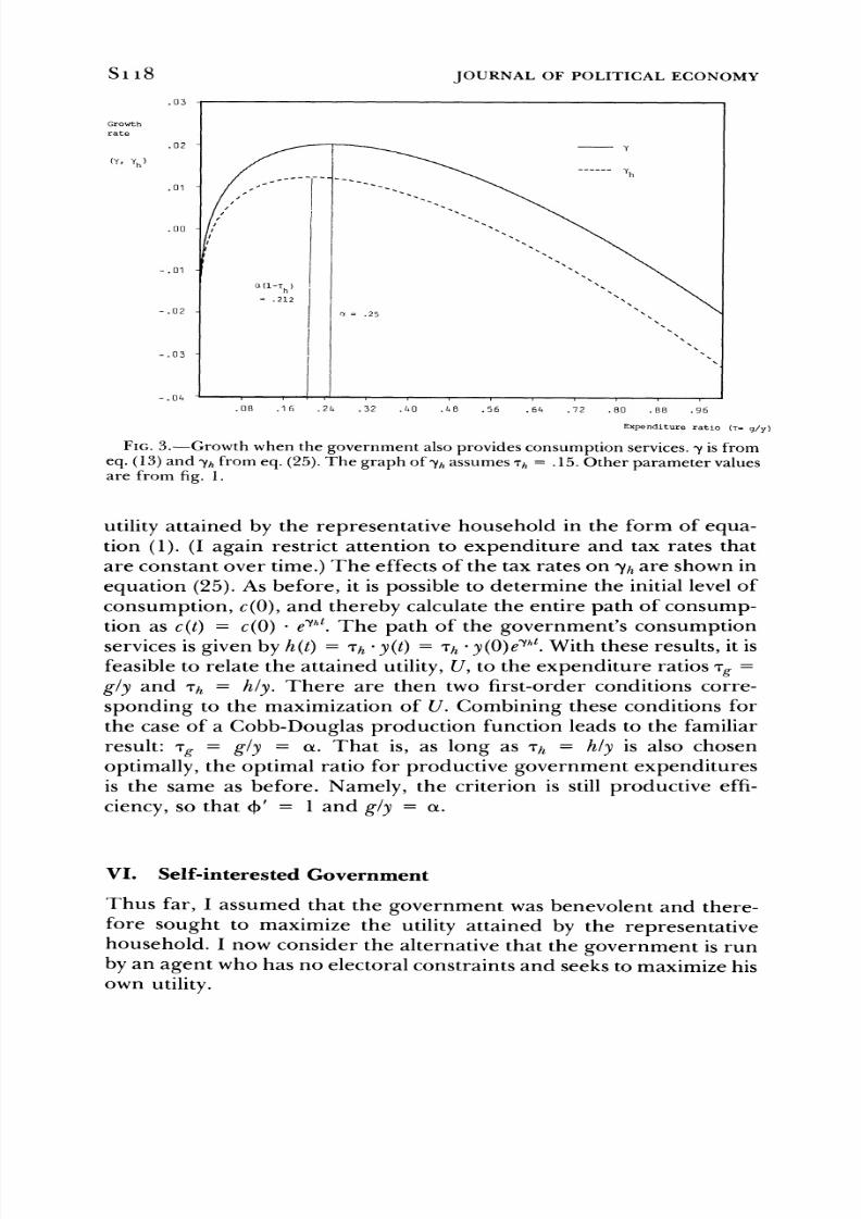
This expression modifies equation (13) in a straightforward manner.The dotted curve in figure 3 shows the relation between Yh and theshare of productive government spending, Tg = gly, taking account of

the positive value of Th = hly. The growth rate lies uniformly belowthe value ry,shown by the solid curve, that would have been chosen if

Th = 0. Figure 4 shows the corresponding saving rates, Sh and s.For a given Th and a Cobb-Douglas production function, it is easy to

show that the value of Tg = gly that maximizes Yh in equation (25) is

(-

TO-). In other words, the growth-maximizing share of produc-tive government spending is smaller if the government is also usingthe income tax to finance other types of spending. However, this

choice turns out not to maximize the utility attained by the represen-

tative household.

Suppose that each household's utility function is given by equation

(23) and that Tg = gly and Th = h/y are set to maximizethe overall



S118 JOURNAL OF POLITICAL ECONOMY

0 3

Growth

rate

- 02 ~ : a.5> "

(y, y

h~~~~~~~~~~~~~~~~y

.212

-.0 2 a .25

-.04

.08 .16 .24 .32 .40 .48 .56 .64 .72 .80 .B8 .96

Expenditure ratio (T= g/y)

FIG. 3.-Growth when the government also provides consumption services. -y s fromeq. (13) and Yhfrom eq. (25). The graph of Yhassumes Th = .15. Other parameter valuesare from fig. 1.

utility attained by the representative household in the form of equa-tion (1). (I again restrict attention to expenditure and tax rates thatare constant over time.) The effects of the tax rates on Yhare shown inequation (25). As before, it is possible to determine the initial level ofconsumption, c(O),and thereby calculate the entire path of consump-tion as c(t) = c(O) eYht. The path of the government's consumptionservices is given by h(t) = Th *y(t) = Th * y(O)eeht. With these results, it isfeasible to relate the attained utility, U, to the expenditure ratios Tg=

gly and Th = hly. There are then two first-order conditions corre-sponding to the maximization of U. Combining these conditions forthe case of a Cobb-Douglas production function leads to the familiar

result: Tg = gly = ot. That is, as long as Th = hly is also chosen

optimally, the optimal ratio for productive government expendituresis the same as before. Namely, the criterion is still productive effi-

ciency, so that 4' = 1 and gly = ot.

VI. Self-interested Government

Thus far, I assumed that the government was benevolent and there-fore sought to maximize the utility attained by the representativehousehold. I now consider the alternative that the government is runby an agent who has no electoral constraints and seeks to maximize hisown utility.




. 5 _

Saving

rate

h .2 5

- .550 | _

-.75

-1 .55

-1 .25

.5 .1 6 .24 .32 .4 .4 .56 .64 .72 .55 .55 .96

Expenditure ratilo (T= g/y )

FIG. 4.-Saving rate when the government also provides consumption services. s isfrom eq. (16); Sh = Yh ' (kly), where Yh is from eq. (25); and Th = .15. Other parametervalues are from fig. 1.

Return to the setting in which all government expenditures, g,

serve as productive inputs for private producers. The governmentstill uses a flat-rate income tax, but instead of automatically balancing

the budget, the government can earn the net revenue

Cg (- )y (26)

where the expenditure ratio gly can differ from the income tax rate T.

The government agent uses his net revenue to purchase the quantityof consumer goods, cg. The agent receives utility from consumption in

the same manner as any household; that is, the flow of utils is u(cg)

from equation (2), and the overall attained utility, U, is given by the

integral in equation (1). In addition, the government agent has the

same discount rate, p, as each household.With constant values for Tand gly, the privately determined growth

rate is still the value y from equation (13). The only difference is that

gly no longer equals T. The government agent's consumption is cg(t) =[T - (gly)] y(O)elt. Therefore, it is possible to write the agent's at-

tained utility as a function of T and gly. For a Cobb-Douglas produc-

tion function, the two first-order conditions for maximization of the

agent's utility lead to the results

T >~- = (X. (27)y




The optimal expenditure rate gly equals a, as in previous models; thatis, the productive-efficiency condition, 4' = 1, still holds. Since thechoice of gly is mainly one of efficient production, the self-interested

government chooses the same value as the benevolent government.Basically, the government agent sets gly = a to maximize the tax basethat he has to work with. Then he is also in the position to set T > gly

to secure the net flow of revenue, cg.

The results in this section parallel those in the preceding one. In

effect, the government agent's consumption, cg, plays the same rolethat the government's consumption services, h, played in the previousmodel. In both cases the presence of these consumption flows doesnot upset the conditions for productive efficiency, which imply (for

Cobb-Douglas technology) that the government's productive expen-ditures are the fraction a of total output. However, the ratio of gov-ernment revenues to output exceeds a in both situations: in one caseto provide consumption to the government agent and in the other toprovide government consumption services to each household.

VII. Some Empirical Implications

The theory has implications for relations between the size of govern-ment and the rates of growth and saving. Because the analysis appliesto steady-state growth paths, the natural empirical application wouldbe to differences in average performance across countries over longperiods of time.

As is usual in empirical investigations, the hypothesized effects of

government policy are easier to assess if the government's actions canbe treated as exogenous. That is, the results are simple if govern-ments randomize their actions and thereby generate useful experi-

mental data. In this case, variations in the share of productive govern-ment expenditures in GDP, gly, affect the growth and saving rates, Yh

and Sh,as shown by the dashed curves in figures 3 and 4, respectively.(The precise curves apply with a proportional income tax and Cobb-

Douglas production function and in settings in which individuals treattheir own allocations of public services, g and h, as given.) As sug-gested before, productive government spending would include theresources devoted to property rights enforcement, as well as activities

that enter directly into production functions. Countries could be ar-rayed along the horizontal axes by the size of gly, and the responses ofy and s would be nonmonotonic, as shown in the figures.

An increase in the share of nonproductive government expendi-tures, say hly in the model of Section V, leads to the types of shiftsshown by the movements from the solid to the dashed curves infigures 3 and 4. For a given value of gly, an increase in hly lowers the




growth and saving rates. These effects arise because a higher hly hasno direct effect on private-sector productivity, but does lead to ahigher income tax rate. Since individuals retain a smaller fraction of

their returns from investment, they have less incentive to invest, andthe economy tends to grow at a lower rate.The predictions are similar for any other differences across coun-

tries that imply that private investors get to retain a smaller fraction oftheir returns from investment. For example, if gly is held fixed, anincrease in the average marginal tax rate or an exogenous worseningof property rights would tend to lower the growth and saving rates.

Aside from problems of measuring public services and the rates ofgrowth and saving, the empirical implementation of the model is

complicated by the endogeneity of the government. Within the theo-retical model (and with a Cobb-Douglas production function), thegovernment sets the share of productive expenditures, gly, to ensureproductive efficiency (4' = 1). Therefore, instead of being arrayedalong the horizontal axes in figures 3 and 4, each government wouldoperate at the same point, gly = a. Within this framework of optimiz-ing governments, cross-sectional variations in gly arise only if a differsfrom country to country.

The parameter a, which measures the productivity of public ser-vices relative to private services, could vary across countries for anumber of reasons. These include geography, the share of agricul-tural production, urban density, and so on. For present purposes it isunnecessary to predict how any specific element would affect a, andtherefore gly, for an optimizing government. As long as the variationsin a are independent of the overall level of productivity,5 the modelpredicts how the induced variations in gly will correlate with those iny The result is that a rise in a, and hence in gly, will reduce Y.6 The

intuition is that an increase in aomeans a shift in relative productivitytoward the factor g that has to be financed by a distorting tax. It is forthis reason that a higher a correlates negatively with y The moregeneral conclusion is that gly and y would show little correlationacross countries because each government goes to the point at whichthe marginal effect of gly on y is close to zero.

For government expenditures that provide only consumption ser-vices, the implications are more straightforward. Variations in the

expenditure share for government consumption, h/y-viewed as gen-erated from differences in preferences for public versus private ser-

' For a Cobb-Douglas production function, ylk = A(glk)c from eq. (10). The condi-tion gik = (g/y) - (y/k) implies ylk = A"' -)(g/y)(XI(l -O. Therefore, the parameterAl('

-- indicates the level of private productivity, y/k, for a given value of gly. The

assumption is that cross-sectional variations in A' (1 are independent of those in at.6 The saving rate s also declines if y > 0.




83. They also found that the share of government investment in GDP

had a statistically insignificant effect on growth, although the point

estimate was positive. However, the last estimate applies when the

ratio of private investment to GDP is held constant.In a recent study of 98 countries in the post-World War II period

(Barro 1989), I modified the Summers-Heston (1988) data on govern-

ment consumption. For the period 1970-85, 1 subtracted the ratios to

GDP of government spending on defense and education from the

ratios reported by Summers and Heston.7 The average value for each

country from 1970 to 1985, denoted by gC/y, was used as a proxy for

the government spending ratio, hly, that enters directly into the utility

function in the theoretical model. The identification of gC with h is

imperfect; for example, police services (a component of gC) wouldinfluence property rights and thereby affect private investment and

growth.

I also measured the ratio of real public gross investment to real

GDP, denoted by g'/y. This public investment corresponds to a stock

of public capital, kg, which generates a flow of services that I view as

comparable to the productive services g in the theory. Thus this em-

pirical measure identifies g with "infrastructure services," such as

transportation, water, electric power, and so on (although hospitalsand schools are also components of public capital). As with the identi-

fication of gC with h, the identification of the flow of services from

public capital with productive government services is imperfect.

In the model, where public capital is combined with private capital

(because public and private production are viewed as governed by the

same production function), the "public capital stock" corresponds to

the fraction of the total stock, k, that produces the public services; that

is, kg = (gly) k. Hence, gly can be measured by the ratio kglk. Since

data on kg and k are unavailable for most countries, I instead approxi-mated kglkby the ratio of gross investments, g1/i, where i is the sum of

private and public investment. The assumptions here are that gly is

constant over time for a single country, and public and private capital

have the same depreciation rates. According to the theory, the rela-

tion of the growth rate Myo g'/i depends on how governments behave.

If governments optimize (go close to the point of maximal growth), My

and g1i1 would show little cross-sectional correlation. On the other

hand, the association would be positive (or negative) if governmentstypically choose too little (or too much) of productive public services.

7For defense and education, the ratios were nominal spending relative to nominal

GDP, whereas the Summers-Heston figures are real spending relative to real GDP. Theimplicit assumption (generated by lack of an alternative) is that the appropriate deflatorfor defense and education is the GDP deflator.




For the 98 countries for which gC/y was measured (Barro 1989, table1), a regression of the average annual growth rate of real per capitaGDP from 1960 to 1985 on a set of explanatory variables8 yielded an

estimated coefficient on gC/y of -.12 (standard error = .03). Thusthere is an indication that an increase in resources devoted to non-productive (but possibly utility-enhancing) government services is as-

sociated with lower per capita growth.For the 76 countries for which data on public investment were

available, the estimated coefficient on g'/i was .014 (s.e. = .022). Thusthe point estimate was positive but insignificantly different from zero.This result is consistent with the hypothesis that the typical countrycomes close to the quantity of public investment that maximizes the

growth rate.If the ratio of public investment to GDP, g'/y, replaces g'li as an

explanatory variable in the growth equation, the estimated coefficientis again positive but insignificant: .13 (s.e. = .10). Moreover, if thevariable ily is also included as a regressor, the estimated coefficient ofily is .073 (s.e. = .039), and that for g1/y becomes - .015 (s.e. = .119).From the standpoint of the theory, the positive coefficient on ily can

be interpreted as the common influence of omitted variables on in-

vestment and growth. In any event, once the total investment ratio il/is held constant, there is no separate effect on growth from the break-down of total investment between private and public components.

These empirical results are representative of ongoing research on

the determinants of economic growth across countries. Aside from

the role of government, this research is currently focusing on theeffects of human capital, market distortions, and political stability.Results of this research will be reported in subsequent papers.

References

Arrow, Kenneth J. "The Economic Implications of Learning by Doing." Rev.

Econ. Studies 29 (June 1962): 155-73.

Arrow, Kenneth J., and Kurz, Mordecai. Public Investment, he Rate of Return,and Optimal Fiscal Policy. Baltimore: Johns Hopkins Univ. Press (for Re-sources for the Future), 1970.

Aschauer, David A. "Is Public Expenditure Productive?" Manuscript. Chi-

cago: Fed. Reserve Bank Chicago, March 1988.

Barro, Robert J. "Economic Growth in a Cross Section of Countries." Work-

ing Paper no. 3120. Cambridge, Mass.: NBER, September 1989.

Barth, James R., and Bradley, Michael D. "The Impact of Government

8 The regression also included the initial (1960) values of real per capita GDP andschool enrollment rates (intended as proxies for initial human capital) and variablesthat measure political stability and market distortions. See Barro (1989) for details.




Spending on Economic Activity." Manuscript. Washington: George Wash-ington Univ., 1987.

Becker, Gary S., and Barro, Robert J. "A Reformulation of the EconomicTheory of Fertility." Q.J.E. 103 (February 1988): 1-25.

Becker, Gary S.; Murphy, Kevin M.; and Tamura, Robert. "Human Capital,Fertility, and Economic Growth."J.P.E., this issue.

Cass, David. "Optimum Growth in an Aggregative Model of Capital Accumu-lation." Rev. Econ. Studies 32 (July 1965): 233-40.

Domar, Evsey D. "Expansion and Employment." A.E.R. 37 (March 1947):34-55.

Grier, Kevin B., and Tullock, Gordon. "An Empirical Analysis of Cross-national Economic Growth, 1950-1980." Manuscript. Pasadena: CaliforniaInst. Tech., December 1987.

Harrod, Roy F. Towardsa Dynamic Economics:Some RecentDevelopments f Eco-

nomic Theoryand Their Application to Policy. London: Macmillan, 1948.Koopmans, Tjalling C. "On the Concept of Optimal Economic Growth." In

The EconometricApproach to Development Planning. Amsterdam: North-Holland, 1965.

Kormendi, Roger C., and Meguire, Philip G. "Macroeconomic Determinantsof Growth: Cross-Country Evidence." J. Monetary Econ. 16 (September1985): 141-63.

Landau, Daniel L. "Government Expenditure and Economic Growth: ACross-Country Study." Southern Econ.J. 49 (January 1983): 783-92.

Lucas, Robert E., Jr. "On the Mechanics of Economic Development."J. Mone-

tary Econ. 22 (July 1988): 3-42.Ramsey, Frank P. "A Mathematical Theory of Saving." Econ.J. 38 (December

1928): 543-59.Rebelo, Sergio. "Long-Run Policy Analysis and Long-Run Growth." J.P.E.

(1991), in press.Romer, Paul M. "Increasing Returns and Long-Run Growth."J.P.E. 94 (Oc-

tober 1986): 1002-37."Capital Accumulation in the Theory of Long Run Growth." In Mod-

ern Business Cycle Theory, edited by Robert J. Barro. Cambridge, Mass.:Harvard Univ. Press, 1989.

. "Endogenous Technological Change."J.P.E., this issue.Samuelson, Paul A. "The Pure Theory of Public Expenditure." Rev. Econ. andStatis. 36 (November 1954): 387-89.

Solow, Robert M. "A Contribution to the Theory of Economic Growth."Q.J.E. 70 (February 1956): 65-94.

Summers, Robert, and Heston, Alan. "Improved International Comparisonsof Real Product and Its Composition: 1950-1980." Rev. Incomeand Wealth30 (June 1984): 207-62.

. "A New Set of International Comparisons of Real Product and PriceLevels: Estimates for 130 Countries, 1950-1985." Rev. Incomeand Wealth34(March 1988): 1-25.

Thompson, Earl A. "Taxation and National Defense."J.P.E. 82 (July/August1974): 755-82.

endogenous model

Documents