Examples of Adaptive MCMCby

Gareth O. Roberts* and Jeffrey S. Rosenthal**

(September, 2006.)

Abstract. We investigate the use of adaptive MCMC algorithms to auto-matically tune the Markov chain parameters during a run. Examples includethe Adaptive Metropolis (AM) multivariate algorithm of Haario et al. (2001),Metropolis-within-Gibbs algorithms for non-conjugate hierarchical models, re-gionally adjusted Metropolis algorithms, and logarithmic scalings. Computersimulations indicate that the algorithms perform very well compared to non-adaptive algorithms, even in high dimension.

1. Introduction.

MCMC algorithms such as the Metropolis-Hastings algorithm (Metropolis et al., 1953;

Hastings, 1970) are extremely widely used in statistical inference, to sample from complicated

high-dimensional distributions. Tuning of associated parameters such as proposal variances

is crucial to achieve efficient mixing, but can also be very difficult.

Adaptive MCMC algorithms attempt to deal with this problem by automatically “learn-

ing” better parameter values of Markov chain Monte Carlo algorithms while they run. In this

paper, we consider a number of examples of such algorithms, including some in high dimen-

sions. We shall see that adaptive MCMC can be very successful at finding good parameter

values with little user intervention.

It is known that adaptive MCMC algorithms will not always preserve stationarity of π(·),see e.g. Rosenthal (2004) and Proposition 3 of Roberts and Rosenthal (2005). However, they

will converge if the adaptions are done at regeneration times (Gilks et al., 1998; Brockwell

and Kadane, 2005), or under various technical conditions about the adaption procedure

(Haario et al., 2001; Atchade and Rosenthal, 2005; Andrieu and Moulines, 2003; Andrieu

and Atchade, 2006). Many of these results also require that the adaptive parameters converge

*Department of Mathematics and Statistics, Fylde College, Lancaster University, Lancaster, LA1 4YF,England. Email: g.o.roberts@lancaster.ac.uk.

**Department of Statistics, University of Toronto, Toronto, Ontario, Canada M5S 3G3. Email:jeff@math.toronto.edu. Web: http://probability.ca/jeff/ Supported in part by NSERC of Canada.

1

to fixed values sufficiently quickly, which runs the risk that they may converge to the “wrong”

values.

Roberts and Rosenthal (2005) proved ergodicity of adaptive MCMC under conditions

which we find simpler to apply, and which do not require that the adaptive parameters

converge. To state their result precisely, suppose the algorithm updates Xn to Xn+1 using

the kernel PΓn , where each fixed kernel Pγ has stationary distribution π(·), but where the

Γn are random indices, chosen iteratively from some collection Y based on past algorithm

output. Write ‖ · · · ‖ for total variation distance, X for the state space, and Mε(x, γ) =

inf{n ≥ 1 : ‖P nγ (x, ·)− π(·)‖ ≤ ε} for the convergence time of the kernel Pγ when beginning

in state x ∈ X . Then Theorem 13 of Roberts and Rosenthal (2005), combined slightly with

their Corollaries 8 and 9 and Theorem 23 and with work of Yang (2006), guarantee that

limn→∞ ‖L(Xn)−π(·)‖ = 0 (asymptotic convergence), and also limn→∞1n

∑ni=1 g(Xi) = π(g)

for all g : X → R with π|g| < ∞ (WLLN), assuming only the Diminishing Adaptation

condition

limn→∞

supx∈X

‖PΓn+1(x, ·)− PΓn(x, ·)‖ = 0 in probability , (1)

and the Bounded Convergence condition

{Mε(Xn, Γn)}∞n=0 is bounded in probability , ε > 0 . (2)

Furthermore, they prove that (2) is satisfied whenever X × Y is finite, or is compact in

some topology in which either the transition kernels Pγ, or the Metropolis-Hastings proposal

kernels Qγ, have jointly continuous densities. (Condition (1) can be ensured directly, by

appropriate design of the adaptive algorithm.)

Such results provide a “hunting license” to look for useful adaptive MCMC algorithms. In

this paper, we shall consider a variety of such algorithms. We shall see that they do indeed

converge correctly, and often have significantly better mixing properties than comparable

non-adaptive algorithms.

2. Adaptive Metropolis (AM).

In this section, we consider a version of the Adaptive Metropolis (AM) algorithm of Haario

et al. (2001). We begin with a d-dimensional target distribution π(·). We perform a Metropo-

lis algorithm with proposal distribution given at iteration n by Qn(x, ·) = N(x, (0.1)2 Id / d)

for n ≤ 2d, while for n > 2d,

Qn(x, ·) = (1− β) N(x, (2.38)2 Σn / d) + β N(x, (0.1)2 Id / d) , (3)

2

where Σn is the current empirical estimate of the covariance structure of the target distri-

bution based on the run so far, and where β is a small positive constant (we take β = 0.05).

It is known from Roberts et al. (1997) and Roberts and Rosenthal (2001) that the pro-

posal N(x, (2.38)2 Σ / d) is optimal in a particular large-dimensional context. Thus, the

N(x, (2.38)2 Σn / d) proposal is an effort to approximate this.

Having β > 0 in (3) ensures that (2) is satisfied. Furthermore, since empirical estimates

change at the nth iteration by only O(1/n), it follows that (1) will also be satisfied. (Haario

et al. instead let Qn(x, ·) = N(x, Σn + ε Id) for small ε, to force c1Id ≤ Σn ≤ c2Id for some

c1, c2 > 0, which also ensures (1) and (2), but we prefer to avoid this.) Hence, this algorithm

will indeed converge to π(·) and satisfy the WLLN.

To test this algorithm, we let π(·) = N(0, M M t), where M is a d× d matrix generated

randomly by letting {Mij}di,j=1 be i.i.d. ∼ N(0, 1). This ensures that the target covariance

matrix Σ = M M t will be highly erratic, so that sampling from π(·) presents a significant

challenge for sampling if the dimension is at all high.

The resulting trace plot of the first coordinate of the Markov chain is presented in Figure 1

for dimension d = 100, and in Figure 2 for dimension d = 200. In both cases, the Markov

chain takes a long time to adaptive properly and settle down to good performance. In

the early stages, the algorithm vastly underestimates the true stationary variance, thus

illustrating the pitfalls of premature diagnoses of MCMC convergence. In the later stages,

by contrast, the algorithm has “learned” how to sample from π(·), and does so much more

successfully.

Another way of monitoring the success of this algorithm’s adapting is as follows. Con-

sider a multidimensional random-walk Metropolis algorithm with proposal covariance matrix

(2.38)2 Σp / d, acting on a normal target distribution with true covariance matrix Σ. The-

orem 5 of Roberts and Rosenthal (2001) prove that it is optimal to take Σp = Σ, and for

other Σp the mixing rate will be slower than this by a suboptimality factor of

b ≡ d

∑di=1 λ−2

i

(∑d

i=1 λ−1i )2

,

where {λi} are the eigenvalues of the matrix Σ1/2p Σ−1/2. Usually we will have b > 1, and the

closer b is to 1, the better.

So how does the AM algorithm perform by this measure? For the run in dimension 100,

the value of this sub-optimality coefficient b begins at the huge value of 193.53, and then even-

tually decreases towards 1, reaching 1.086 after 500,000 iterations, and 1.024 after 1,000,000

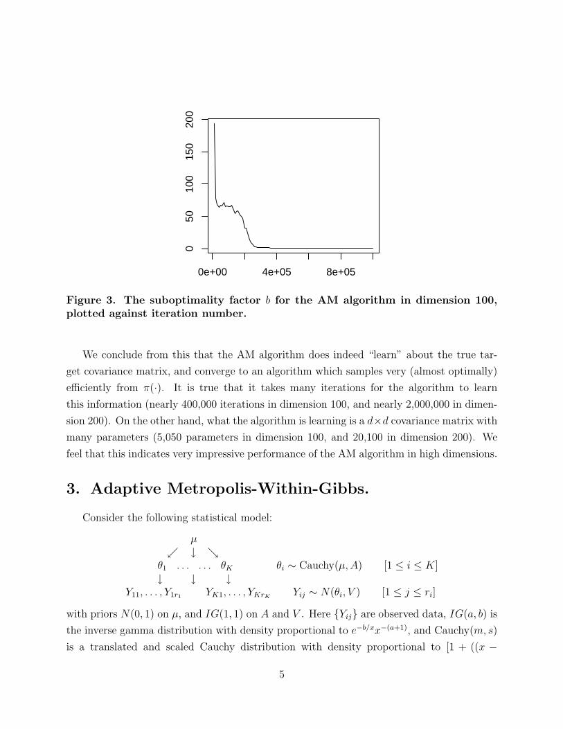
iterations (Figure 3). In dimension 200, the value of b is even more erratic, starting around

183,000 and oscillating wildly before decreasing to about 1.04.

3

0e+00 4e+05 8e+05

−2

−1

01

2

Figure 1. The first coordinate of the AM Markov chain in dimension 100, plottedagainst iteration number.

0 1000000 2500000

−4

−2

02

4

Figure 2. The first coordinate of the AM Markov chain in dimension 200, plottedagainst iteration number.

4

0e+00 4e+05 8e+05

050

100

150

200

Figure 3. The suboptimality factor b for the AM algorithm in dimension 100,plotted against iteration number.

We conclude from this that the AM algorithm does indeed “learn” about the true tar-

get covariance matrix, and converge to an algorithm which samples very (almost optimally)

efficiently from π(·). It is true that it takes many iterations for the algorithm to learn

this information (nearly 400,000 iterations in dimension 100, and nearly 2,000,000 in dimen-

sion 200). On the other hand, what the algorithm is learning is a d×d covariance matrix with

many parameters (5,050 parameters in dimension 100, and 20,100 in dimension 200). We

feel that this indicates very impressive performance of the AM algorithm in high dimensions.

3. Adaptive Metropolis-Within-Gibbs.

Consider the following statistical model:

µ↙ ↓ ↘

θ1 . . . . . . θK θi ∼ Cauchy(µ, A) [1 ≤ i ≤ K]↓ ↓ ↓

Y11, . . . , Y1r1 YK1, . . . , YKrKYij ∼ N(θi, V ) [1 ≤ j ≤ ri]

with priors N(0, 1) on µ, and IG(1, 1) on A and V . Here {Yij} are observed data, IG(a, b) is

the inverse gamma distribution with density proportional to e−b/xx−(a+1), and Cauchy(m, s)

is a translated and scaled Cauchy distribution with density proportional to [1 + ((x −

5

m)/s)2]−1. This model gives rise to a posterior distribution π(·) on the (K + 3)-dimensional

vector (A, V, µ, θ1, . . . , θK), conditional on the observed data {Yij}.We take K = 500, and let the ri vary between 5 and 500. The resulting model is too

complicated for analytic computation, and far too high-dimensional for numerical integra-

tion. Furthermore, the presence of the Cauchy (as opposed to Normal) distribution destroys

conjugacy, and thus makes a classical Gibbs sampler (as in Gelfand and Smith, 1990) infea-

sible. Instead, a Metropolis-within-Gibbs algorithm (Metropolis et al., 1953; Tierney, 1994)

seems appropriate.

Such an algorithm might proceed as follows. We consider each of the 503 variables in

turn. For each, we propose updating its value by adding a N(0, σ2) increment. That proposal

is then accepted or rejected according to the usual Metropolis ratio. This process is repeated

many times, allowing the variables to hopefully converge in distribution to π(·). But how

should σ2 be chosen? Should it be different for different variables? How can we feasibly

determine appropriate scalings in such high dimension?

To answer these questions, an adaptive algorithm can be used. We proceed as follows.

For each of the variables i [1 ≤ i ≤ K + 3], we create an associated variable lsi giving

the logarithm of the standard deviation to be used when proposing a normal increment to

variable i. We begin with lsi = 0 for all i (corresponding to unit proposal variance). After

the nth “batch” of 50 iterations, we update each lsi by adding or subtracting an adaption

amount δ(n). The adapting attempts to make the acceptance rate of proposals for variable i

as close as possible to 0.44 (which is optimal for one-dimensional proposals in certain settings,

cf. Roberts et al., 1997; Roberts and Rosenthal, 2001). Specifically, we increase lsi by δ(n)

if the fraction of acceptances of variable i was more than 0.44 on the nth batch, or decrease

lsi by δ(n) if it was less.

Condition (1) is satisfied provided δ(n) → 0; we take δ(n) = min(0.01, n−1/2). To

ensure (2), we can specify a global maximal parameter value M < ∞, and restrict each lsi

to the interval [−M, M ]. In practice, the lsi stabilise nicely so this isn’t actually needed.

To test this adaptive algorithm, we generate independent test date Yij ∼ N(i− 1, 102),

for 1 ≤ i ≤ 500 and 1 ≤ j ≤ ri. For such data, our simulations show that the scaling

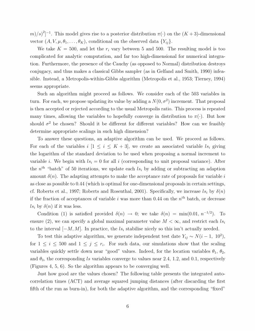
variables quickly settle down near “good” values. Indeed, for the location variables θ1, θ2,

and θ3, the corresponding ls variables converge to values near 2.4, 1.2, and 0.1, respectively

(Figures 4, 5, 6). So the algorithm appears to be converging well.

Just how good are the values chosen? The following table presents the integrated auto-

correlation times (ACT) and average squared jumping distances (after discarding the first

fifth of the run as burn-in), for both the adaptive algorithm, and the corresponding “fixed”

6

0 50000 150000 250000

0.0

0.5

1.0

1.5

2.0

2.5

Figure 4. The log proposal standard deviation ls1 corresponding to theMetropolis-within-Gibbs variable θ1, plotted against batch number.

0 50000 150000 250000

0.0

0.4

0.8

1.2

Figure 5. The log proposal standard deviation ls2 corresponding to theMetropolis-within-Gibbs variable θ2, plotted against batch number.

7

0 50000 150000 250000

0.00

0.10

0.20

0.30

Figure 6. The log proposal standard deviation ls3 corresponding to theMetropolis-within-Gibbs variable θ3, plotted against batch number.

algorithm where each lsi is fixed at 0:

Variable ri Algorithm ACT Avr Sq Distθ1 5 Adaptive 2.59 14.932θ1 5 Fixed 31.69 0.863θ2 50 Adaptive 2.72 1.508θ2 50 Fixed 7.33 0.581θ3 500 Adaptive 2.72 0.150θ3 500 Fixed 2.67 0.147

This table shows that, when comparing adaptive to fixed algorithms, for variables θ1

and θ2, the autocorrelation times are significantly smaller (better) and the average square

jumping distances are significantly larger (better), Thus, adapting has significantly improved

the MCMC algorithm, by automatically choosing appropriate proposal scalings separately for

each coordinate. For variable θ3 the performance of the two algorithms is virtually identical,

which is not surprising since (Figure 6) the optimal log proposal standard deviation happens

to be very close to 0 in that case.

In summary, this adaptive algorithm appears to correctly scale the proposal standard

deviations, leading to a Metropolis-within-Gibbs algorithm which mixes much faster than

a naive one with unit proposal scalings. Coordinates are improved wherever possible, and

8

are left about the same when they happen to already be optimal. This works even in high

dimensions, and does not require any direct user intervention or high-dimensional insight.

Remark. A different component-wise adaptive scaling method, the Single Component

Adaptive Metropolis (SCAM) algorithm, is presented in Haario et al. (2005). That algorithm,

which resembles the Adaptive Metropolis algorithm of Haario et al. (2001), is very interesting

and promising, but differs significantly from ours since the SCAM adapting is done based

on the empirical variance of each component based on the run so far.

4. State-Dependent Scalings.

We next consider examples of full-dimensional Metropolis-Hastings algorithms, where

the proposal distribution is given by Q(x, ·) = N(x, σ2x), i.e. such that the proposal vari-

ance depends on the current state x ∈ X . For such an algorithm, according to the usual

Metropolis-Hastings formula (Hastings, 1970), a proposal from x to y is accepted with prob-

ability

α(x, y) = min[1,

π(y)

π(x)(σx/σy)

d exp (− 1

2(x− y)2(σ−2

y − σ−2x ))

]. (4)

As a first case, we let X = R, and π(·) = N(0, 1). We consider proposal kernels of the

form

Qa,b(x, ·) = N

(x, ea

(1 + |x|exp(π)

)b)

,

where π is our current empirical estimate of π(g) where g(x) = log(1 + |x|). (We divide by

exp(π) to make the choices of a and b “orthogonal” in some sense.) After the nth batch of

100 iterations, we update a by adding or subtracting δ(n) in an effort to, again, make the

acceptance rate as close as possible to 0.44. We also add or subtract δ(n) to b to make the

acceptance rate in the regions {x ∈ X : log(1 + |x|) > π} and {x ∈ X : log(1 + |x|) ≤ π}as equal as possible. We also again restrict a and b to [−M, M ] for some global parameter

M < ∞. As before, if δ(n) → 0 and M < ∞, then conditions (1) and (2) are satisfied, so

we must have ‖L(Xn)− π(·)‖ → 0.

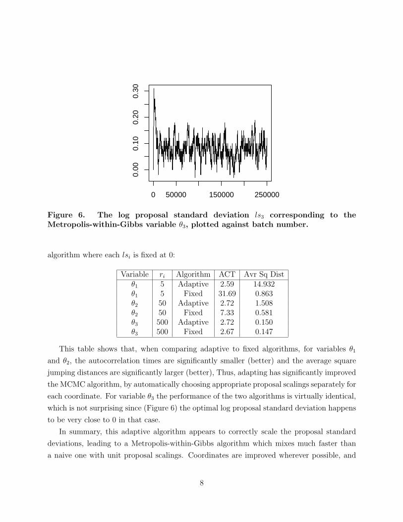
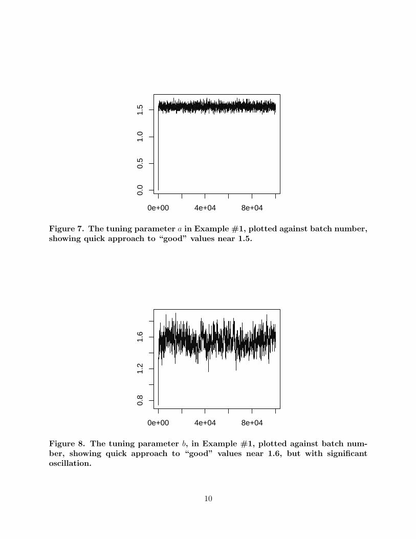
So how does this algorithm perform in practice? Empirical expected values quickly

converge to their true values, showing excellent mixing. Furthermore, the tuning parameters

a and b quickly find their “good” values (Figures 7 and 8), though they do continue to

oscillate due to the extremely slow rate at which δ(n) → 0.

To determine how well the adaptive algorithm is performing, we compare its integrated

autocorrelation time and average squared jumping distance to corresponding non-adaptive

9

0e+00 4e+04 8e+04

0.0

0.5

1.0

1.5

Figure 7. The tuning parameter a in Example #1, plotted against batch number,showing quick approach to “good” values near 1.5.

0e+00 4e+04 8e+04

0.8

1.2

1.6

Figure 8. The tuning parameter b, in Example #1, plotted against batch num-ber, showing quick approach to “good” values near 1.6, but with significantoscillation.

10

algorithms, having either fixed constant variance σ2 (including the optimal constant value,

(2.38)2), and to the corresponding variable-variance algorithm. The results are as follows:

Algorithm Acceptance Rate ACT Avr Sq DistAdaptive (as above) 0.456 2.63 0.769

σ2 = exp(−5) 0.973 49.92 0.006σ2 = exp(−1) 0.813 8.95 0.234

σ2 = 1 0.704 4.67 0.450σ2 = (2.38)2 0.445 2.68 0.748σ2 = exp(5) 0.237 7.22 0.305

σ2x = e1.5

(1+|x|

0.534822

)1.60.456 2.58 0.778

We see that our adaptive scheme is much better than arbitrarily-chosen fixed-variance

algorithms, slightly better than the optimally-chosen fixed-variance algorithm (5th line),

and nearly as good as an ideally-chosen variable-σ2 scheme (bottom line). This is quite

impressive, since we didn’t do any manual tuning of our algorithm at all other than telling

the computer to seek a 0.44 acceptance rate.

While these functional forms of σ2x seem promising, it is not clear how to generalise them

to higher dimensional problems. Instead, we next consider a different algorithm in which

the σ2x are piecewise constant over various regions of the state space.

5. Regional Adaptive Metropolis Algorithm (RAMA).

The Regional Adaptive Metropolis Algorithm (RAMA) begins by partitioning the state

space X into a finite number of disjoint regions: X = X1•∪ . . .

•∪Xm. The algorithm then

proceeds by running a Metropolis algorithm with proposal Q(x, ·) = N(x, exp(2 ai)) when-

ever x ∈ Xi. Thus, if x ∈ Xi and y ∈ Xj, then σ2x = e2ai and σ2

y = e2aj , and it follows from (4)

that a proposal from x to y is accepted with probability

α(x, y) = min[1,

π(y)

π(x)exp (d(ai − aj)−

1

2(x− y)2[exp(−2aj)− exp(−2ai)])

].

The adaptions proceed as follows, in an effort to make the acceptance probability close to

0.234 in each region. (Such an acceptance rate is optimal in certain high-dimensional settings;

see Roberts et al., 1997; Roberts and Rosenthal, 1998, 2001; Bedard, 2006a, 2006b.) For

1 ≤ i ≤ d, the parameter a1 is updated by, after the nth batch of 100 iterations, considering

the fraction of acceptances of those proposals which originated from Xi. If that fraction is

less than 0.234 then ai is decreased by δ(n), while if it is more than ai is increased by δ(n).

Then, if ai > M we set ai = M , while if ai < −M we set ai = −M . Finally, if there were no

11

0e+00 4e+04 8e+04

−0.

4−

0.3

−0.

2−

0.1

0.0

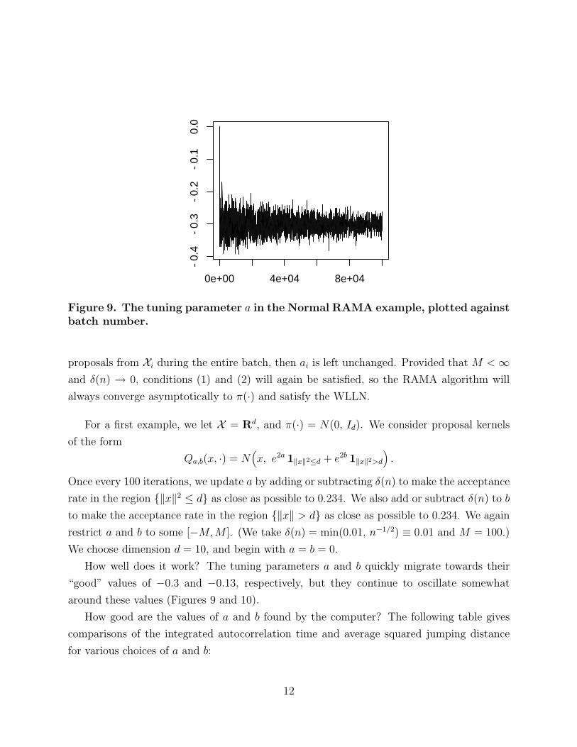
Figure 9. The tuning parameter a in the Normal RAMA example, plotted againstbatch number.

proposals from Xi during the entire batch, then ai is left unchanged. Provided that M < ∞and δ(n) → 0, conditions (1) and (2) will again be satisfied, so the RAMA algorithm will

always converge asymptotically to π(·) and satisfy the WLLN.

For a first example, we let X = Rd, and π(·) = N(0, Id). We consider proposal kernels

of the form

Qa,b(x, ·) = N(x, e2a 1‖x‖2≤d + e2b 1‖x‖2>d

).

Once every 100 iterations, we update a by adding or subtracting δ(n) to make the acceptance

rate in the region {‖x‖2 ≤ d} as close as possible to 0.234. We also add or subtract δ(n) to b

to make the acceptance rate in the region {‖x‖ > d} as close as possible to 0.234. We again

restrict a and b to some [−M, M ]. (We take δ(n) = min(0.01, n−1/2) ≡ 0.01 and M = 100.)

We choose dimension d = 10, and begin with a = b = 0.

How well does it work? The tuning parameters a and b quickly migrate towards their

“good” values of −0.3 and −0.13, respectively, but they continue to oscillate somewhat

around these values (Figures 9 and 10).

How good are the values of a and b found by the computer? The following table gives

comparisons of the integrated autocorrelation time and average squared jumping distance

for various choices of a and b:

12

0e+00 4e+04 8e+04

−0.

20−

0.10

0.00

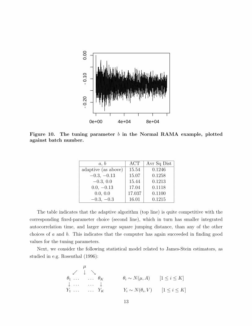
Figure 10. The tuning parameter b in the Normal RAMA example, plottedagainst batch number.

a, b ACT Avr Sq Distadaptive (as above) 15.54 0.1246

−0.3, −0.13 15.07 0.1258−0.3, 0.0 15.44 0.12130.0, −0.13 17.04 0.11180.0, 0.0 17.037 0.1100

−0.3, −0.3 16.01 0.1215

The table indicates that the adaptive algorithm (top line) is quite competitive with the

corresponding fixed-parameter choice (second line), which in turn has smaller integrated

autocorrelation time, and larger average square jumping distance, than any of the other

choices of a and b. This indicates that the computer has again succeeded in finding good

values for the tuning parameters.

Next, we consider the following statistical model related to James-Stein estimators, as

studied in e.g. Rosenthal (1996):

µ↙ ↓ ↘

θ1 . . . . . . θK θi ∼ N(µ, A) [1 ≤ i ≤ K]↓ . . . . . . ↓

Y1 . . . . . . YK Yi ∼ N(θi, V ) [1 ≤ i ≤ K]

13

0e+00 4e+04 8e+04

−3.

4−

3.3

−3.

2−

3.1

−3.

0

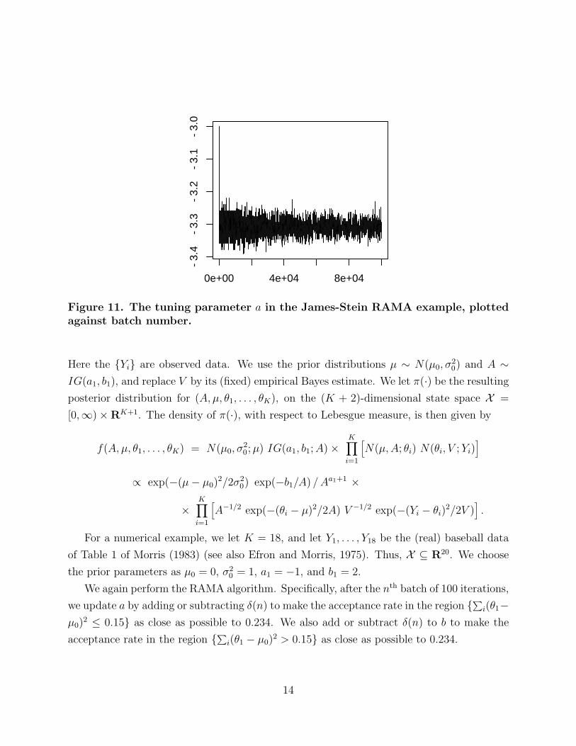
Figure 11. The tuning parameter a in the James-Stein RAMA example, plottedagainst batch number.

Here the {Yi} are observed data. We use the prior distributions µ ∼ N(µ0, σ20) and A ∼

IG(a1, b1), and replace V by its (fixed) empirical Bayes estimate. We let π(·) be the resulting

posterior distribution for (A, µ, θ1, . . . , θK), on the (K + 2)-dimensional state space X =

[0,∞)×RK+1. The density of π(·), with respect to Lebesgue measure, is then given by

f(A, µ, θ1, . . . , θK) = N(µ0, σ20; µ) IG(a1, b1; A)×

K∏i=1

[N(µ, A; θi) N(θi, V ; Yi)

]

∝ exp(−(µ− µ0)2/2σ2

0) exp(−b1/A) /Aa1+1 ×

×K∏

i=1

[A−1/2 exp(−(θi − µ)2/2A) V −1/2 exp(−(Yi − θi)

2/2V )].

For a numerical example, we let K = 18, and let Y1, . . . , Y18 be the (real) baseball data

of Table 1 of Morris (1983) (see also Efron and Morris, 1975). Thus, X ⊆ R20. We choose

the prior parameters as µ0 = 0, σ20 = 1, a1 = −1, and b1 = 2.

We again perform the RAMA algorithm. Specifically, after the nth batch of 100 iterations,

we update a by adding or subtracting δ(n) to make the acceptance rate in the region {∑i(θ1−µ0)

2 ≤ 0.15} as close as possible to 0.234. We also add or subtract δ(n) to b to make the

acceptance rate in the region {∑i(θ1 − µ0)2 > 0.15} as close as possible to 0.234.

14

0e+00 4e+04 8e+04

−3.

35−

3.25

−3.

15−

3.05

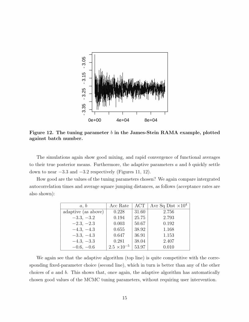
Figure 12. The tuning parameter b in the James-Stein RAMA example, plottedagainst batch number.

The simulations again show good mixing, and rapid convergence of functional averages

to their true posterior means. Furthermore, the adaptive parameters a and b quickly settle

down to near −3.3 and −3.2 respectively (Figures 11, 12).

How good are the values of the tuning parameters chosen? We again compare intergrated

autocorrelation times and average square jumping distances, as follows (acceptance rates are

also shown):

a, b Acc Rate ACT Avr Sq Dist ×104

adaptive (as above) 0.228 31.60 2.756−3.3, −3.2 0.194 25.75 2.793−2.3, −2.3 0.003 50.67 0.192−4.3, −4.3 0.655 38.92 1.168−3.3, −4.3 0.647 36.91 1.153−4.3, −3.3 0.281 38.04 2.407−0.6, −0.6 2.5 ×10−5 53.97 0.010

We again see that the adaptive algorithm (top line) is quite competitive with the corre-

sponding fixed-parameter choice (second line), which in turn is better than any of the other

choices of a and b. This shows that, once again, the adaptive algorithm has automatically

chosen good values of the MCMC tuning parameters, without requiring user intervention.

15

Remarks.

1. In our simulations, the condition M < ∞ has never been necessary, since RAMA has

never tried to push any of the {aj} towards unbounded values. Indeed, we conjecture

that under appropriate regularity assumptions (e.g. if the densities are jointly continu-

ous), condition (2) will be satisfied automatically due to drifting of the parameters ai

back to reasonable values due to the adaptive process (cf. Roberts and Rosenthal, 2005,

Corollary 14).

2. If some value aj is much too large, then α(x, y) may be very small for all y ∈ Xj and x 6∈Xj. This means that the region Xj may virtually never be entered, so that aj will remain

virtually constant, leading to isolation of Xj and thus very poor convergence. Hence, it is

important with RAMA to begin with sufficiently small values of the {ai}. Alternatively,

it might be wise to decrease each ai slightly (rather than leaving it unchanged) after each

batch in which there were no proposals from Xi.

3. The version of RAMA presented here requires that the user specify the regions {Xi}mi=1

by hand. However, it may also be possible to have the computer automatically select

appropriate regions, by e.g. doing a preliminary run with fixed proposal variance, and

then grouping together state space subsets which appear to have similar acceptance rates.

4. One can ask whether the results of Roberts et al. (1997) carry over to RAMA, and

whether equal acceptance rates on different regions (as sought by RAMA) truly leads

to optimality. We believe this to be true quite generally, but can only prove it for very

specific settings (e.g. birth-death processes). The method of proof of Roberts et al. (see

also Bedard, 2006a, 2006b) appears to carry over away from the region boundaries, but

the behaviour at the region boundaries is more complicated.

5. If we set δ(n) to a constant, as opposed to having δ(n) → 0, then condition 1 might fail,

so the chain might not converge to π(·). On the other hand, the chain together with the

parameter values {aj} is jointly Markovian, and under appropriate scaling may have its

own joint diffusion limit. It would be interesting (Stewart, 2006) to study that diffusion

limit, to e.g. see how much asymptotic error results from failing to satisfy (1).

6. To Log or Not To Log.

Suppose π is the density function for a real-valued random variable W . Then if π is

heavy-tailed, then it may be advantageous to take logarithms, i.e. to instead consider the

density function for W ≡ log W . This leads to the question, when is it advantageous to

consider W in place of W? Once again, adaptive algorithms can provide insights into this

16

question.

To avoid problems of negative or near-negative values, we modify the logarithm function

and instead consider the function

`(w) ≡ sgn(w) log(1 + |w|) ,

where sgn(w) = 1 for w > 0, and sgn(w) = −1 for w < 0. The function ` is an increasing,

continuously differentiable mapping from R onto R, with inverse `−1(w) = sgn(w) (e|w|− 1),

and graph as follows:

−10 −5 0 5 10

−4

−2

02

4

Figure 13. Graph of the modified log function `.

If π is the density for W , and W = log(W ), then taking Jacobians shows that the density

for W is given by π(w) = e|w| π(e|w| − 1).

A result of Mengersen and Tweedie (1996) says, essentially, that a random-walk Met-

ropolis (RWM) algorithm for a density π will be geometrically ergodic if and only if π has

exponential or sub-exponential tails, i.e. satisfies

log π(x)− log π(y) ≥ α(y − x) , y > x ≥ x1 (5)

for some x1 > 0 and α > 0 (and similarly for y < x ≤ −x1). (A similar result holds in

multidimensions, cf. Roberts and Tweedie, 1996.) But if π on R satisfies (5), then so does

π, since if y > x ≥ − log(α) + β ≥ x1 > 0, then

log π(x)− log π(y) = (x− y) + log π(ex − 1)− log π(ey − 1)

17

≥ (x− y) + α((ey − 1)− (ex − 1)) = −(y − x) + αex(ey−x − 1)

≥ −(y − x) + αex(y − x) = (y − x)(αex − 1) ≥ (y − x)(eβ − 1) .

Hence, (5) is satisfied for π with α = eβ − 1. In fact, by making β arbitrarily large, we can

make α as large as we like, showing that the tails of π are in fact sub-exponential.

This suggests that, at least as far as geometric ergodicity is concerned, it is essentially

always better to work with π than with π. As a specific example, if π is the standard Cauchy

distribution, then RWM on π is not geometrically ergodic, but RWM on π is.

Despite this evidence in favour of log transforms for RWM, it is not clear that taking

logarithms (or applying `) necessarily helps with the quantitative convergence of RWM. To

investigate this, we use an adaptive algorithm.

Specifically, given π, we consider two different algorithms: one a RWM on π, and the

other a RWM on π, each using proposal distributions of the form Q(x, ·) = N(x, σ2). After

the nth batch of 100 iterations, we allow each version to adapt its own scaling parameter σ

by adding or subtracting δ(n) to log(σ), in an effort to achieve acceptance rate near 0.44 for

each version. Then, once every 100 batches, we consider whether to switch versions (i.e., to

apply ` if we currently haven’t, or to undo ` if we currently have), based on whether the

current average square jumping distance is smaller than that from the last time we used the

other version. (We force the switch to the other version if it fails 100 times in succession, to

avoid getting stuck forever with just one version.)

How does this adaptive algorithm work in practice? In the following table we considered

three different one-dimensional symmetric target distributions: a standard Normal, a stan-

dard Cauchy, and a Uniform[−100, 100]. For each target, we report the percentage of the

time that the adaptive algorithm spent on the logged density π (as opposed to the regular

density π). We also report the mean value of the log proposal standard deviation for both

the regular and the logged RWM versions.

Target Log % lsreg lslog

Normal 3.62% 2.52 2.08Cauchy 99.0% 3.49 2.66Uniform 4.95% 6.66 2.65

We see from this table that, for the Normal and Uniform distributions, the adaptive

algorithm saw no particular advantage to taking logarithms, and indeed stayed in the regular

(unlogged) π version the vast majority of the time. On the other hand, for the Cauchy target,

the algorithm uses the logged π essentially as much as possible. This shows that this adaptive

18

algorithm is able to distinguish between when taking logs is helpful (e.g. for the heavy-tailed

Cauchy target), and when it is not (e.g. for the light-tailed Normal and Uniform targets).

For multidimensional target distributions, it is possible to take logs (or apply the function

`) separately to each coordinate. Since lighter tails are still advantageous in multidimensional

settings (Roberts and Tweedie, 1996), it seems likely to be advantageous to apply ` to

precisely those coordinates which correspond to heavy tails in the target distribution. In

high dimensions, this cannot feasibly be done by hand, but an adaptive algorithm could still

do it automatically. Such multidimensional versions of this adaptive logarithm algorithm

appear worthy of further investigation.

7. Conclusion.

This paper has considered automated tuning of MCMC algorithms, especially Metropolis-

Hastings algorithms, with quite positive results.

For example, for Metropolis-within-Gibbs algorithms, our simulations indicate that: (1)

The choice of proposal variance σ2 is crucial to the success of the algorithm. (2) Good

values of σ2 can vary greatly from one coordinate to the next. (3) There are far too many

coordinates to be able to select good values of σ2 for each coordinate by hand. (4) Adaptive

methods can be used to get the computer to find good values of σ2 automatically. (5) If done

carefully, the adaptive methods can be provably ergodic, and quite effective in practice, thus

allowing for good tuning and rapid convergence of MCMC algorithms that would otherwise

be impractical.

Similar observations apply to the Adaptive Metropolis algorithm, the issue of applying

logarithms to target distributions, etc.

Overall, we feel that these results indicate the widespread applicability of adaptive

MCMC algorithms to many different MCMC settings, including complicated high-dimensional

distributions. We hope that this paper will inspire users of MCMC to experiment with adap-

tive algorithms in their future applications. As a start, all of the software used to run the

algorithms described herein is freely available at probability.ca/adapt.

Acknowledgements. We thank Sylvia Richardson for a very helpful suggestion.

19

REFERENCES

C. Andrieu and Y.F. Atchade (2005), On the efficiency of adaptive MCMC algorithms.Preprint.

C. Andrieu and E. Moulines (2003), On the ergodicity properties of some adaptive MarkovChain Monte Carlo algorithms. Preprint.

Y.F. Atchade and J.S. Rosenthal (2005), On Adaptive Markov Chain Monte Carlo Algo-rithms. Bernoulli 11, 815–828.

M. Bedard (2006a), Weak convergence of Metropolis algorithms for non-iid target distribu-tions. Preprint.

M. Bedard (2006b), Optimal acceptance rates for Metropolis algorithms: moving beyond0.234. Preprint.

A.E. Brockwell and J.B. Kadane (2005), Identification of regeneration times in MCMC sim-ulation, with application to adaptive schemes. J. Comp. Graph. Stat. 14, 436–458.

B. Efron and C. Morris (1975), Data analysis using Stein’s estimator and its generalizations.J. Amer. Stat. Assoc., Vol. 70, No. 350, 311-319.

A.E. Gelfand and A.F.M. Smith (1990), Sampling based approaches to calculating marginaldensities. J. Amer. Stat. Assoc. 85, 398-409.

W.R. Gilks, G.O. Roberts, and S.K. Sahu (1998), Adaptive Markov Chain Monte Carlo. J.Amer. Stat. Assoc. 93, 1045–1054.

H. Haario, E. Saksman, and J. Tamminen (2001), An adaptive Metropolis algorithm. Bernoulli7, 223–242.

H. Haario, E. Saksman, and J. Tamminen (2005), Componentwise adaptation for high di-mensional MCMC. Comput. Stat. 20, 265–274.

W.K. Hastings (1970), Monte Carlo sampling methods using Markov chains and their appli-cations. Biometrika 57, 97–109.

K.L. Mengersen and R.L. Tweedie (1996), Rates of convergence of the Hastings and Metro-polis algorithms. Ann. Statist. 24, 101–121.

N. Metropolis, A. Rosenbluth, M. Rosenbluth, A. Teller, and E. Teller (1953), Equations ofstate calculations by fast computing machines. J. Chem. Phys. 21, 1087–1091.

C. Morris (1983), Parametric empirical Bayes confidence intervals. Scientific Inference, DataAnalysis, and Robustness, 25-50.

G.O. Roberts, A. Gelman, and W.R. Gilks (1997), Weak convergence and optimal scaling ofrandom walk Metropolis algorithms. Ann. Appl. Prob. 7, 110–120.

G.O. Roberts and J.S. Rosenthal (1998), Optimal scaling of discrete approximations toLangevin diffusions. J. Roy. Stat. Soc. B 60, 255–268.

20

G.O. Roberts and J.S. Rosenthal (2001), Optimal scaling for various Metropolis-Hastingsalgorithms. Stat. Sci. 16, 351–367.

G.O. Roberts and J.S. Rosenthal (2005), Coupling and Ergodicity of Adaptive MCMC.Preprint.

G.O. Roberts and R.L. Tweedie (1996), Geometric Convergence and Central Limit Theoremsfor Multidimensional Hastings and Metropolis Algorithms. Biometrika 83, 95–110.

J.S. Rosenthal (1996), Analysis of the Gibbs sampler for a model related to James-Steinestimators. Stat. and Comp. 6, 269–275.

J.S. Rosenthal (2004), Adaptive MCMC Java Applet. Available at:

http://probability.ca/jeff/java/adapt.html

A. Stewart (2006), Personal communication.

C. Yang (2006), On adaptive MCMC. PhD thesis, University of Toronto. Work in progress.

21