adaptive mcmc with bayesian optimization -...

Adaptive MCMC with Bayesian Optimization

Nimalan Mahendran Ziyu Wang Firas Hamze Nando de FreitasUBC UBC D-Wave Systems UBC

Abstract

This paper proposes a new randomized strat-egy for adaptive MCMC using Bayesian op-timization. This approach applies to non-differentiable objective functions and tradesoff exploration and exploitation to reducethe number of potentially costly objectivefunction evaluations. We demonstrate thestrategy in the complex setting of samplingfrom constrained, discrete and densely con-nected probabilistic graphical models where,for each variation of the problem, one needsto adjust the parameters of the proposalmechanism automatically to ensure efficientmixing of the Markov chains.

1 Introduction

A common line of attack for solving problems inphysics, statistics and machine learning is to drawsamples from probability distributions π(·) that areonly known up to a normalizing constant. Markovchain Monte Carlo (MCMC) algorithms are often thepreferred method for accomplishing this sampling task,see e.g. Andrieu et al. (2003) and Robert & Casella(1998). Unfortunately, these algorithms typically haveparameters that must be tuned in each new situationto obtain reasonable mixing times. These parame-ters are often tuned by a domain expert in a time-consuming and error-prone manual process. AdaptiveMCMC methods have been developed to automaticallyadjust the parameters of MCMC algorithms. We referthe reader to three recent and excellent comprehensivereviews of the field (Andrieu & Thoms, 2008; Atchadeet al., 2009; Roberts & Rosenthal, 2009).

Adaptive MCMC methods based on stochastic approx-imation have garnered the most interest out of the vari-

Appearing in Proceedings of the 13th International Con-ference on Artificial Intelligence and Statistics (AISTATS)2010, Chia Laguna Resort, Sardinia, Italy. Volume 9 ofJMLR: W&CP 9. Copyright 2010 by the authors.

ous adaptive MCMC methods for two reasons. Firstly,they can be shown to be theoretically valid. That is,the Markov chain is made inhomogenous by the de-pendence of the parameter updates upon the historyof the Markov chain, but its ergodicity can be ensured(Andrieu & Robert, 2001; Andrieu & Moulines, 2006;Saksman & Vihola, 2010). For example, Theorem 5of Roberts & Rosenthal (2007) establishes two simpleconditions to ensure ergodicity: (i) the non-adaptivesampler has to be uniformly ergodic and (ii) the levelof adaptation must vanish asymptotically. These con-ditions can be easily satisfied for discrete state spacesand finite adaptation.

Secondly, adaptive MCMC algorithms based onstochastic approximation have been shown to workwell in practice (Haario et al., 2001; Roberts & Rosen-thal, 2009; Vihola, 2010). However, there are somelimitations to the stochastic approximation approach.Some of the most successful samplers rely on know-ing either the optimal acceptance rate or the gradientof some objective function of interest. Another disad-vantage is that these stochastic approximation meth-ods may require many iterations. This is particularlyproblematic when the objective function being opti-mized by the adaptation mechanism is costly to evalu-ate. Finally, gradient approaches tend to be local andhence they can get trapped in local optima when theMarkov chains are run for a finite number of steps inpractice.

This paper aims to overcome some of these limitations.It proposes the use of Bayesian optimization (Brochuet al., 2009) to tune the parameters of the Markovchain. The proposed approach, Bayesian-optimizedMCMC, has a few advantages over adaptive methodsbased on stochastic approximation.

Bayesian optimization does not require that the ob-jective function be differentiable. This enables us tobe much more flexible in the design of the adapta-tion mechanisms. We use the area under the auto-correlation function up to a specific lag as the objectivefunction in this paper. This objective has been sug-gested previously by Andrieu & Robert (2001). How-ever, the computation of gradient estimates for this

751


objective is very involved and far from trivial (Andrieu& Robert, 2001). We believe this is one of the mainreasons why practitioners have not embraced this ap-proach. Here, we show that this objective can be eas-ily optimized with Bayesian optimization. We arguethat Bayesian optimization endows the designer withgreater freedom in the design of adaptive strategies.

Bayesian optimization also has the advantage that itis explicitly designed to trade off exploration and ex-ploitation and is implicitly designed to minimize thenumber of expensive evaluations of the objective func-tion (Brochu et al., 2009; Lizotte et al., 2011).

Another important property of Bayesian-optimizedMCMC is that it does not use a specific setting for theparameters of the proposal distribution, but rather adistribution over parameter settings with probabilitiesestimated during the adaptation process. Indeed, wefind that a randomized policy over a set of parametersettings mixes faster than a specific parameter valuefor the models considered in this paper.

Bayesian optimization has been used with MCMC inRasmussen (2003) with the intent of approximatingthe posterior with a surrogate function to minimize thecost of hybrid Monte Carlo evaluations. The intent inthis paper is instead to adapt the parameters of theMarkov chain to improve mixing.

To demonstrate MCMC adaptation with Bayesian op-timization, we study the problem of adapting a sam-pler for constrained discrete state spaces proposed re-cently by Hamze & de Freitas (2010). The sampleruses augmentation of the state space in order to makelarge moves in discrete state space. In this sense, thesampler is similar to the Hamiltonian (hybrid) MonteCarlo for continuous state spaces (Duane et al., 1987;Neal, 2010). Although these samplers typically onlyhave two parameters, these are very tricky to tune evenby experts. Moreover, every time we make a changeto the model, the expert is again required to spendtime tuning the parameters. This is often the casewhen dealing with sampling from discrete probabilis-tic graphical models, where we often want to vary thetopology of the graph as part of the data analysis andexperimentation process. In the experimental sectionof this paper, we will discuss several Ising models, alsoknown as Boltzmann machines, and show that indeedthe optimal parameters vary significantly for differentmodel topologies.

There are existing consistency results for Bayesian op-timization (Vasquez & Bect, 2008; Srinivas et al., 2010;Bull, 2011). These results in combination with the factthat we focus on discrete distributions are sufficientfor ensuring ergodicity of our adaptive MCMC schemeunder vanishing adaptation. However, the type of

Bayesian optimization studied in this paper relies onlatent Gaussian processes whose covariance grows asthe Markov chain progresses. For very large chains,it becomes prohibitive to invert the covariance matrixof the Gaussian process. Thus, for practical reasons,we adopt instead a two-stage adaptation mechanism,where we first adapt the chain for a finite numberof steps and then use the most promising parame-ter values to run the chain again with a mixture ofMCMC kernels (Andrieu & Thoms, 2008). Althoughthis adaptation strategy increases the computationalcost of the MCMC algorithm, we argue that this costis much lower than the cost of having a human in theloop choosing the parameters.

2 Adaptive MCMC

The Metropolis-Hasting (MH) algorithm is the keybuilding block for most MCMC methods (Andrieuet al., 2003). It draws samples from a target distri-bution π(·) by proposing a move from x(t) to y(t+1)

according to a parameterized proposal distributionqθ(y

(t+1)|x(t)) and either accepting it (x(t+1) = y(t+1))with probability equal to the acceptance ratio

α(x(t) → y(t+1)) = min

{π(y(t+1))qθ(x

(t)|y(t+1))

π(x(t))qθ(y(t+1)|x(t)), 1

}

or rejecting it (x(t+1) = x(t)) otherwise.

The parameters of the proposal, θ ∈ Θ ⊆ Rd, can havea large influence on sampling performance. For exam-ple, we will consider constrained discrete probabilis-tic models in our experiments, where changes to theconnectivity patterns among the random variables willrequire different parameter settings. We would like tohave an approach that can adjust these parametersautomatically for all possible connectivity patterns.

Several methods have been proposed to adapt MCMCalgorithms. Instead of discussing all of these, we referthe reader to the comprehensive reviews of Andrieu& Thoms (2008); Atchade et al. (2009); Roberts &Rosenthal (2009). One can adapt parameters otherthan those of the proposal distribution in certain situ-ations, but for the sake of simplicity, we focus here onadapting the proposal distribution.

One of the most successful adaptive MCMC algorithmswas introduced by Haario et al. (2001) and several ex-tensions were proposed by Andrieu & Thoms (2008).This algorithm is restricted to the adaptation of themultivariate random walk Metropolis algorithm withGaussian proposals. It is motivated by a theoreti-cal result regarding the optimal covariance matrix ofa restrictive version of this sampler (Gelman et al.,1996). This adaptive algorithm belongs to the familyof stochastic approximation methods.

752

Nimalan Mahendran, Ziyu Wang, Firas Hamze, Nando de Freitas

Some notation needs to be introduced to briefly de-scribe stochastic approximation, which will also beuseful later when we replace the stochastic approxi-mation method with Bayesian optimization. Let Xi ={x(t)}it=1 denote the full set of samples up to itera-tion i of the MH algorithm and Yi = {y(t)}it=1 be thecorresponding set of proposed samples. x(0) is the ini-tial sample. We will group these samples into a singlevariable Mi = (x(0),Xi,Yi). Let g(θ) be the meanfield of the stochastic approximation that may only beobserved noisily as G(θi,Mi). When optimizing anobjective function h(θ), this mean field correspondsto the gradient of this objective, that is g(θ) = ∇h(θ).Adaptive MCMC methods based on stochastic approx-imation typically use the following Robbins-Monro up-date:

θi+1 = θi + γi+1G (θi,Mi+1) , (1)

where γi+1 is the step-size. This recursive estimateconverges almost surely to the roots of g(θ) as i→∞under suitable conditions.

We are concerned with the adaptation of discrete mod-els in this paper. The optimal acceptance rates are un-known. It is also not clear what objective function oneshould optimize to adjust the parameters of the pro-posal distribution. One possible choice, as mentionedin the introduction, is to use the auto-correlation func-tion up to a certain lag. Intuitively, this objectivefunction seems to be suitable for the adaptation taskbecause it is used in practice to assess convergence.Unfortunately, it is difficult to obtain efficient esti-mates of the gradient of this objective (Andrieu &Robert, 2001). To overcome this difficulty, we intro-duce Bayesian optimization in the following section.

3 Bayesian Optimization forAdaptive MCMC

The proposed adaptive strategy consists of two phases:adaptation and sampling. In the adaptation phaseBayesian optimization is used to construct a random-ized policy. In the sampling phase, a mixture ofMCMC kernels selected according to the learned ran-domized policy is used to explore the target distri-bution. The two phases are discussed in more detailsubsequently.

3.1 Adaptation Phase

Our objective function for adaptive MCMC cannot beevaluated analytically. However, noisy observations ofits value can be obtained by running the Markov chainfor a few steps with a specific choice of parameters θi.Bayesian optimization in the adaptive MCMC setting

proposes a new candidate θi+1 by approximating theunknown function using the entire history of noisy ob-servations and a prior distribution over functions. Theprior distribution used in this paper is a Gaussian pro-cess.

The noisy observations are used to obtain the predic-tive distribution of the Gaussian process. An expectedutility function derived in terms of the sufficient statis-tics of the predictive distribution is optimized to selectthe next parameter value θi+1. The overall procedureis shown in Algorithm 1. We refer readers to Brochuet al. (2009) and Lizotte (2008) for in-depth reviewsof Bayesian optimization.

Algorithm 1 Adaptive MCMC with Bayesian Opt.

1: for i = 1, 2, . . . , I do2: Run Markov chain for L steps with parameters θi.3: Use the drawn samples to obtain a noisy evaluation

of the objective function: zi = h(θi) + ε.4: Augment the data D1:i = {D1:i−1, (θi, zi)}.5: Update the GP’s sufficient statistics.6: Find θi+1 by optimizing an acquisition function:

θi+1 = arg maxθ u(θ|D1:i).

7: end for

The unknown objective function h(·) is assumed to bedistributed according to a Gaussian process with meanfunction m(·) and covariance function k(·, ·):

h(·) ∼ GP (m(·), k(·, ·)).

We adopt a zero mean function m(·) = 0 and ananisotropic Gaussian covariance that is essentially thepopular ARD kernel (Rasmussen & Williams, 2006):

k(θj , θk) = exp

(−1

2(θj − θk)Tdiag(ψ)−2(θj − θk)

)

where ψ ∈ Rd is a vector of hyper-parameters. TheGaussian process is a surrogate model for the true ob-jective, which typically involves intractable expecta-tions with respect to the invariant distribution and theMCMC transition kernels. We describe the objectivefunction used in this work in Section 3.3.

We assume that the noise in the measurements isGaussian: zi = h(θi) + ε, ε ∼ N (0, σ2

η). It is possi-ble to adopt other noise models (Diggle et al., 1998).Our Gaussian process has hyper-parameters ψ andση. These hyper-parameters are typically computedby maximizing the likelihood (Rasmussen & Williams,2006). In Bayesian optimization, we can use Latin hy-percube designs to select an initial set of parametersand then proceed to maximize the likelihood of thehyper-parameters iteratively (Ye, 1998; Santner et al.,2003). This is the approach followed in our experi-ments. However, a good alternative is to use either

753


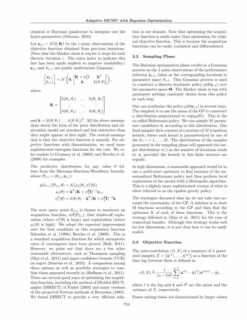
classical or Bayesian quadrature to integrate out thehyper-parameters (Osborne, 2010).

Let z1:i ∼ N (0,K) be the i noisy observations of theobjective function obtained from previous iterations.(Note that the Markov chain is run for L steps for eachdiscrete iteration i. The extra index to indicate thisfact has been made implicit to improve readability.)z1:i and hi+1 are jointly multivariate Gaussian:

[z1:ihi+1

]= N

(0,

[K + σ2

ηI kT

k k(θ, θ)

]),

where

K =

k(θ1, θ1) . . . k(θ1, θi)

.... . .

...k(θi, θ1) . . . k(θi, θi)

and k = [k(θ, θ1) . . . k(θ, θi)]T . All the above assump-

tions about the form of the prior distribution and ob-servation model are standard and less restrictive thanthey might appear at first sight. The central assump-tion is that the objective function is smooth. For ob-jective functions with discontinuities, we need moresophisticated surrogate functions for the cost. We re-fer readers to Gramacy et al. (2004) and Brochu et al.(2009) for examples.

The predictive distribution for any value θ fol-lows from the Sherman-Morrison-Woodbury formula,where D1:i = (θ1:i, z1:i):

p(hi+1|D1:i, θ) = N (µi(θ), σ2i (θ))

µi(θ) = kT (K + σ2ηI)−1z1:i

σ2i (θ) = k(θ, θ)− kT (K + σ2

ηI)−1k

The next query point θi+1 is chosen to maximize anacquisition function, u(θ|D1:i), that trades-off explo-ration (where σ2

i (θ) is large) and exploitation (whereµi(θ) is high). We adopt the expected improvementover the best candidate as this acquisition functionSchonlau et al. (1998); Brochu et al. (2009). This isa standard acquisition function for which asymptoticrates of convergence have been proved (Bull, 2011).However, we point out that there are a few otherreasonable alternatives, such as Thompson sampling(May et al., 2011) and upper confidence bounds (UCB)on regret (Srinivas et al., 2010). A comparison amongthese options as well as portfolio strategies to com-bine them appeared recently in (Hoffman et al., 2011).There are several good ways of optimizing the acquisi-tion function, including the method of DIvided RECT-angles (DIRECT) of Finkel (2003) and many versionsof the projected Newton methods of Bertsekas (1982).We found DIRECT to provide a very efficient solu-

tion in our domain. Note that optimizing the acquisi-tion function is much easier than optimizing the origi-nal objective function. This is because the acquisitionfunctions can be easily evaluated and differentiated.

3.2 Sampling Phase

The Bayesian optimization phase results in a Gaussianprocess on the I noisy observations of the performancecriterion z1:I , taken at the corresponding locations inparameter space θ1:I . This Gaussian process is usedto construct a discrete stochastic policy p(θ|z1:I) overthe parameter space Θ. The Markov chain is run withparameter settings randomly drawn from this policyat each step.

One can synthesize the policy p(θ|z1:I) in several ways.The simplest is to use the mean of the GP to constructa distribution proportional to exp(µ(θ)). This is theso-called Boltzmann policy. We can sample M param-eter candidates θi according to this distribution. Ourfinal sampler then consists of a mixture ofM transitionkernels, where each kernel is parameterized by one ofthe θi, i = 1, . . . ,M . The distribution of the samplesgenerated in the sampling phase will approach the tar-get distribution π(·) as the number of iterations tendsto ∞ provided the kernels in this finite mixture areergodic.

In high dimensions, a reasonable approach would be touse a multi-start optimizer to find maxima of the un-normalized Boltzmann policy and then perform localexploration of the modes with a Metropolis algorithm.This is a slightly more sophisticated version of what isoften referred to as the epsilon greedy policy.

The strategies discussed thus far do not take into ac-count the uncertainty of the GP. A solution is to drawM functions according to the GP and then find theoptimizer θi of each of these functions. This is thestrategy followed in (May et al., 2011) for the case ofcontextual bandits. Although this strategy works wellfor low dimensions, it is not clear how it can be easilyscaled.

3.3 Objective Function

The auto-correlation r(l,X ) of a sequence of n gener-ated samples X = {x(1), . . . ,x(n)} as a function of thetime lag between them is defined as

r(l,X ) , 1

(n− l)δ2n−l∑

t=1

(x(t) − x̄)T (x(t+l) − x̄),

where l is the lag and x̄ and δ2 are the mean and thevariance of X , respectively.

Faster mixing times are characterized by larger values

754


of a(lmax,X ) = 1 − (lmax−1)

∑lmax

l=1 |r(l,X )|. We usethis property to construct the criterion for Bayesianoptimization as follows. Let Ei be the last i sampledstates (the energies in the experimental section). Theperformance criterion is obtained by taking the av-erage of a(·) over a sliding window within the lastL samples, down to a minimum window size of 25:

1L−25+1

∑Li=25 a(i, Ei).

4 Application to Constrained DiscreteDistributions

The Intracluster Move (IM) sampler was recently pro-posed to generate samples from notoriously-hard con-strained Boltzmann machines in (Hamze & de Freitas,2010). This sampler has two parameters (one contin-uous and the other discrete) that the authors stateto be difficult to tune. This and the recent growinginterest in discrete Boltzmann machines in machinelearning motivated us to apply the proposed Bayesian-optimized MCMC method to this problem.

Boltzmann machines are described in Ackley et al.(1985). Let xi ∈ {0, 1} denote the i-th random vari-able in the model. The Boltzmann distribution is givenby

π(x) , 1

Z(β)e−βE(x), (2)

where Z(β) ,∑

x∈S e−βE(x) is the normalizing con-

stant, β is a temperature parameter and E(x) ,−∑i,j xiJijxj−

∑i bixi is the energy function. Boltz-

mann machines also have coupling parameters J andb that are assumed to be known.

Let Sn(c) be the subset of the states that are at exactlyHamming distance n away from a reference state c.The distribution πn,c(x) is the restriction of π(x) to

Sn(c). πn,c(x) has Zn(β, c) ,∑

x∈Sn(c) e−βE(x) as its

normalizing constant and is defined as

πn,c(x) ,{

1Zn(β,c)

e−βE(x) if x ∈ Sn(c)

0 otherwise(3)

The rest of the paper makes c implicit and uses thesimplified notation Sn, πn(x) and Zn(β). These con-straints on the states are used in statistical physics andin regularized statistical models (Hamze & de Freitas,2010).

The IM sampler proposes a new state y(t+1) ∈ Snfrom an original state x(t) ∈ Sn using self-avoidingwalks (SAWs) and has parameters θ = (k, γ), wherek ∈ L , {1, 2, . . . , kmax} is the length of each SAWand γ ∈ G , [0, γmax] is the energy-biasing parameter.k determines the size, in terms of the number of bits

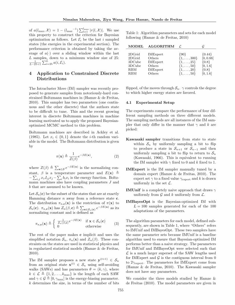
Table 1: Algorithm parameters and sets for each modelfollowing (Hamze & de Freitas, 2010)

MODEL ALGORITHM L G

2DGrid IMExpert {90} {0.44}2DGrid Others {1, . . . , 300} [0, 0.88]3DCube IMExpert {1, . . . , 25} {0.8}3DCube Others {1, . . . , 50} [0, 1.6]RBM IMExpert {1, . . . , 20} {0.8}RBM Others {1, . . . , 50} [0, 1.6]

flipped, of the moves through Sn. γ controls the degreeto which higher energy states are favored.

4.1 Experimental Setup

The experiments compare the performance of four dif-ferent sampling methods on three different models.The sampling methods are all instances of the IM sam-pler that only differ in the manner that γ and k arepicked:

Kawasaki sampler transitions from state to statewithin Sn by uniformly sampling a bit to flipto produce a state in Sn+1 or Sn−1 and thenuniformly sampling a bit to flip to return to Sn(Kawasaki, 1966). This is equivalent to runningthe IM sampler with γ fixed to 0 and k fixed to 1.

IMExpert is the IM sampler manually tuned by adomain expert (Hamze & de Freitas, 2010). Theexpert set γ to a fixed value γexpert and k is drawnuniformly in the set L.

IMUnif is a completely naive approach that draws γuniformly from G and k uniformly from L.

IMBayesOpt is the Bayesian-optimized IM withL = 100 samples generated for each of the 100adaptations of the parameters.

The algorithm parameters for each model, defined sub-sequently, are shown in Table 1, where “Others” refersto IMUnif and IMBayesOpt. These two samplers havethe same parameter sets because IMUnif is a baselinealgorithm used to ensure that Bayesian-optimized IMperforms better than a naive strategy. The parametersfor IMUnif and IMBayesOpt were selected such thatL is a much larger superset of the SAW lengths usedfor IMExpert and G is the contiguous interval from 0to 2γexpert. The parameters for IMExpert come from(Hamze & de Freitas, 2010). The Kawasaki samplerdoes not have any parameters.

We consider the three models studied by Hamze &de Freitas (2010). The model parameters are given in

755


Table 2: Model parameters from Hamze & de Freitas(2010). n refers to the number of bits that are set to1 out of the total number. β−1 is the temperature.

MODEL β−1 SIZE n

2DGrid 2.27 60× 60 1800 of 36003DCube 1.0 9× 9× 9 364 of 729RBM 1.0 |v| = 784, |h| = 500 428 of 1284

Table 2. Note that n refers to the Hamming distancefrom states in Sn to the reference state c. The refer-ence state c was set to the ground state where noneof the bits are set to 1. This is particularly intuitivein machine learning applications, where we might notwant more than a small percentage of the binary vari-ables on as part of a regularization or variable selectionstrategy.

Ferromagnetic 2D grid Ising model: The ferro-magnetic 2D grid Ising model is made up of nodesarranged in a planar and rectangular grid with con-nections between the nodes on one boundary to thenodes on the other boundary for each dimension (i.e.periodic boundaries), also known as a square toroidalgrid. Hence, each node has exactly four neighbours.The interaction weights, Jij , are all 1 and the biases,bi, are all 0. The temperature 2.27 is the critical tem-perature of the model.

Frustrated 3D cube Ising model: The frustrated3D cube Ising model is made up of nodes arrangedin a topology that is the three-dimensional analogueof the two-dimensional grid with periodic boundaries.Hence, each node has exactly six neighbours. The in-teraction weights, Jij , are uniformly sampled from theset {−1, 1} and the biases, bi, are all 0.

Restricted Boltzmann machine (RBM): TheRBM has a bipartite graph structure, with h hiddennodes in one partition and v visible nodes in the other.The interaction weights Jij and biases bi are exactlythe same as in Hamze & de Freitas (2010) and corre-spond to local Gabor-like filters that capture regular-ities in perceptual inputs.

Each sampler was run five times with 9 × 104 stepsfor each run. IMBayesOpt had an additional 104 stepsfor an adaptation phase consisting of 100 adaptationsof 100 samples each. IMBayesOpt was not penalizedfor the computational overhead involved in these addi-tional steps because it is seen as being far cheaper thanhaving the IM sampler parameters tuned manually.

All of the algorithms have a burn-in phase consistingof the first 104 samples generated in the corresponding

sampling phase. The burn-in phase was not includedin the computation of the auto-correlation functionsin figures 1, 3 and 5.

IMBayesOpt begins its sampling phase in the samestarting state as all of the other samplers, even thoughit would most likely be in a low energy state at theend of its adaptation phase. This ensures that thecomparison of the sampling methods is fair.

4.2 Results

4.2.1 Ferromagnetic 2D grid Ising model

IMExpert and IMBayesOpt both have very similarmean ACFs, as indicated in Figure 1. IMUnif suffersfrom many long strings of consecutive proposal rejec-tions. This is evident from the many intervals wherethe sampled state energy does not change.

0 100 200 300 400 5000

0.1

0.2

0.3

0.4

0.5

0.6

0.7

0.8

0.9

1

Lag

Abs

auto

corr

IMBayesOptIMExpertIMUnifKawasakiSampler

0 500 1000 1500 2000 2500 3000 3500 4000Steps

6000

5500

5000

4500

4000

3500

3000

2500

Energ

y

IMExpertIMUnifKawasakiSamplerIMBayesOpt

Figure 1: [Top] Mean and error bars of the auto-correlation function of the energies of the 2D grid Isingmodel samples. [Bottom] Average of the energies.

Figure 2 suggests that γ is much more important tothe performance of the IM sampler than the SAWlengths for this model, especially at large SAW lengths.One of the highest probability points in the GP corre-sponds to the parameters chosen by Hamze & de Fre-itas (2010) (γ = 0.44, k = 90). Figure 2 also shows

756


50

100

150

200

2500.0

0.1

0.2

0.3

0.4

0.5

0.6

0.7

0.8

-1.010-0.786-0.561-0.337-0.1120.1120.3370.5610.7861.010

0.2

0.1

0.0

0.1

0.2

0.3

0.4

0.5

50

100

150

200

250

300 0.0

0.1

0.2

0.3

0.4

0.5

0.6

0.7

0.8

0.0002.6675.3338.00010.66713.33316.00018.66721.33324.000

Figure 2: [Top] Mean function of the GP on Θ, learnedby IMBayesOpt for the 2D grid Ising model. An av-erage over the five trials is shown. [Bottom] The cor-responding unnormalized discrete policy used for sam-pling with the mixture of MCMC Kernels.

M = 1000 samples drawn from the Boltzmann pol-icy. The MCMC results are for this policy. The sameprocedure is adopted for the other models.

4.2.2 Frustrated 3D cube Ising model

Figure 3 shows that IMUnif now performs far worsethan the IMExpert and IMBayesOpt, implying thatthe extremely rugged energy landscape of the 3D cubeIsing model makes manual tuning a non-trivial andnecessary process. IMBayesOpt performs very simi-larly to IMExpert, but is automatically tuned withoutany human intervention.

The GP mean function in Figure 4 suggests that SAWlengths should not be longer than k = 25, as found inHamze & de Freitas (2010). Both IMExpert and IM-BayesOpt are essentially following the same strategyand performing well, while the performance of IMUnifconfirms that tuning is important for the 3D model.

0 50 100 150 200 250 300 350 400 450 5000

0.1

0.2

0.3

0.4

0.5

0.6

0.7

0.8

0.9

1

Lag

Abs

auto

corr


0 500 1000 1500 2000 2500 3000 3500 4000Steps

1400

1200

1000

800

600

400

200

0

200

Energ

y


Figure 3: [Top] Mean and error bars of the auto-correlation function of the energies of the 3D cube Isingmodel samples. [Bottom] Average of the energies.

10

20

30

400.0

0.2

0.4

0.6

0.8

1.0

1.2

1.4

-1.010-0.786-0.561-0.337-0.1120.1120.3370.5610.7861.010

0.0

0.1

0.2

0.3

0.4

0.5

0.6

Figure 4: Mean function of the GP on Θ, learned byIMBayesOpt for the 3D cube Ising model. An averageover the five trials is shown.

757


0 100 200 300 400 5000

0.1

0.2

0.3

0.4

0.5

0.6

0.7

0.8

0.9

1

Lag

Abs

auto

corr


0 500 1000 1500 2000 2500 3000 3500 4000Steps

6000

5500

5000

4500

4000

3500

3000

2500

Energ

y


Figure 5: [Top] Mean and error bars of the auto-correlation function of the energies of the RBM sam-ples. [Bottom] Average of the energies.

4.2.3 Restricted Boltzmann Machine (RBM)

Hamze & de Freitas (2010) find that IMExpert experi-ences a rapid dropoff in ACF, but this dropoff is exag-gerated by the inclusion of the burn-in phase. Figure 5shows a much more modest dropoff when the burn-inphase is left out of the ACF computation. However,it still corroborates the claim in Hamze & de Freitas(2010) that IMExpert performs far better than theKawasaki sampler.

Figure 5 shows that IMExpert does not perform muchbetter than IMUnif. The variance of IMExpert’s ACFis also much higher than any of the other methods.IMBayesOpt performs significantly better than any ofthe other methods, including manual tuning by a do-main expert.

The GP mean function in figure 6 suggests that SAWlengths greater than 20 can be used and are as ef-fective as shorter ones, whereas Hamze & de Freitas(2010) only pick SAW lengths between 1 and 20. Thisdiscrepancy is an instance where Bayesian-optimizedMCMC has found better parameters than a domainexpert.

10

20

30

400.0

0.2

0.4

0.6

0.8

1.0

1.2

1.4

-1.010-0.786-0.561-0.337-0.1120.1120.3370.5610.7861.010

0.2

0.1

0.0

0.1

0.2

0.3

0.4

0.5

0.6

Figure 6: Mean function of the GP on Θ, learned byIMBayesOpt for the RBM. An average over the fivetrials is shown.

5 Conclusions

Experiments were conducted to assess Bayesian op-timization for adaptive MCMC. Hamze & de Freitas(2010) state that it is easiest to manually tune the 2Dgrid Ising model and that tuning the 3D cube Isingmodel is more challenging. Manual tuning significantlyimproves the performance of the IM sampler for thesecases, but Bayesian-optimized MCMC is able to real-ize the same gains without any human intervention.This automatic approach surpasses the human expertfor the RBM model.

Bayesian optimization is a general method for adapt-ing the parameters of any MCMC algorithm. It createsnew opportunities for research on adaptive MCMCthat focuses on optimization and computational is-sues. Several challenges remain, including scaling tohigher-dimensions, improving the observation models,designing suitable objective functions, and providingfinite time theoretical guarantees on the mixing time ofthe adaptive chains. Very recently, we demonstratedthat the technique scales reasonably well to moder-ately high dimensions (Hamze et al., 2011; Hoffmanet al., 2011) and that it can be applied to adapt Hamil-tonian (hybrid) Monte Carlo, when using predictionaccuracy on test data as the objective function (Wang& de Freitas, 2011). In this latter work, we replaceGPs with Bayesian parametric models so as to allowfor infinite (asymptotically vanishing) adaptation.

Acknowledgements

We are grateful to Eric Brochu, Arnaud Doucet andDavid Dunson for insightful comments that greatly im-proved this work, supported by MITACS and NSERC.

758


References

Ackley, David H., Hinton, Geoffrey E., and Sejnowski,Terrence J. A learning algorithm for Boltzmann ma-chines. Cognitive Science, 9:147–169, 1985.

Andrieu, Christophe and Moulines, Eric. On the er-godicity properties of some adaptive MCMC algo-rithms. The Annals of Applied Probability, 16(3):1462–1505, 2006.

Andrieu, Christophe and Robert, Christian. Con-trolled MCMC for optimal sampling. Technical Re-port 0125, Cahiers de Mathematiques du Ceremade,Universite Paris-Dauphine, 2001.

Andrieu, Christophe and Thoms, Johannes. A tutorialon adaptive MCMC. Statistics and Computing, 18(4):343–373, 2008.

Andrieu, Christophe, de Freitas, Nando, Doucet, Ar-naud, and Jordan, Michael I. An Introduction toMCMC for Machine Learning. Machine Learning,50(1):5–43, January 2003.

Atchade, Yves, Gersende Fort, Eric Moulines, andPriouret, Pierre. Adaptive Markov chain MonteCarlo: Theory and methods. Technical report, Uni-versity of Michigan, 2009.

Bertsekas, Dimitri P. Projected Newton methodsfor optimization problems with simple constraints.SIAM J. on Control and Optimization, 20(2):221–246, 1982.

Brochu, Eric, Cora, Vlad M., and de Freitas, Nando.A tutorial on Bayesian optimization of expensivecost functions, with application to active user mod-eling and hierarchical reinforcement learning. Tech-nical Report TR-2009-23, Department of ComputerScience, University of British Columbia, November2009.

Bull, Adam D. Convergence rates of efficientglobal optimization algorithms. Arxiv preprintarXiv:1101.3501, 2011.

Diggle, P. J., Tawn, J. A., and Moyeed, R. A. Model-based geostatistics. Journal of the Royal Statisti-cal Society. Series C (Applied Statistics), 47(3):299–350, 1998.

Duane, Simon, Kennedy, A. D., Pendleton, Brian J.,and Roweth, Duncan. Hybrid Monte Carlo. Physicsletters B, 195(2):216–222, 1987.

Finkel, Daniel E. DIRECT Optimization AlgorithmUser Guide. 2003.

Gelman, Andrew, Roberts, Gareth O., and Gilks,Walter R. Efficient Metropolis jumping rules. InBernado, J. M. et al. (eds.), Bayesian Statistics, vol-ume 5, pp. 599. OUP, 1996.

Gramacy, Robert B., Lee, Herbert K. H., andMacready, William G. Parameter space explorationwith Gaussian process trees. In International Con-ference on Machine Learning, pp. 45–52, 2004.

Haario, Heikki, Saksman, Eero, and Tamminen,Johanna. An adaptive Metropolis algorithm.Bernoulli, 7(2):223–242, 2001.

Hamze, Firas and de Freitas, Nando. Intraclustermoves for constrained discrete-space MCMC. InUncertainty in Artificial Intelligence, pp. 236–243,2010.

Hamze, Firas, Wang, Ziyu, and de Freitas, Nando.Self-avoiding random dynamics on integer complexsystems. Technical Report arXiv:1111.5379v2, 2011.

Hoffman, Matt, Brochu, Eric, and de Freitas, Nando.Portfolio allocation for Bayesian optimization. InUncertainty in Artificial Intelligence, pp. 327–336,2011.

Kawasaki, Kyozi. Diffusion constants near the criticalpoint for time-dependent Ising models. i. Phys. Rev.,145(1):224–230, 1966.

Lizotte, Daniel. Practical Bayesian Optimization. PhDthesis, University of Alberta, Edmonton, Alberta,Canada, 2008.

Lizotte, Daniel, Greiner, Russell, and Schuurmans,Dale. An experimental methodology for responsesurface optimization methods. Journal of Global Op-timization, pp. 1–38, 2011.

May, Benedict C, Korda, Nathan, Lee, Anthony, andLeslie, David S. Optimistic Bayesian sampling incontextual bandit problems. 2011.

Neal, Radford M. MCMC using Hamiltonian dynam-ics. Handbook of Markov Chain Monte Carlo, 2010.

Osborne, Michael. Bayesian Gaussian Processes forSequential Prediction, Optimisation and Quadra-ture. PhD thesis, University of Oxford, Oxford, UK,2010.

Rasmussen, Carl E. and Williams, Christopher. Gaus-sian Processes for Machine Learning. MIT Press,2006.

Rasmussen, Carl Edward. Gaussian processes to speedup hybrid Monte Carlo for expensive Bayesian inte-grals. Bayesian Statistics, 7:651–659, 2003.

Robert, Christian P. and Casella, George. Monte CarloStatistical Methods. Springer, 1st edition, 1998.

Roberts, Gareth O. and Rosenthal, Jeffrey S. Couplingand ergodicity of adaptive Markov chain MonteCarlo algorithms. Journal of applied probability, 44(2):458–475, 2007.

Roberts, Gareth O. and Rosenthal, Jeffrey S. Exam-ples of adaptive MCMC. Journal of Computationaland Graphical Statistics, 18(2):349–367, 2009.

759


Saksman, Eero and Vihola, Matti. On the ergodicityof the adaptive Metropolis algorithm on unboundeddomains. Annals of Applied Probability, 20(6):2178– 2203, 2010.

Santner, T J, Williams, B, and Notz, W. The Designand Analysis of Computer Experiments. Springer,2003.

Schonlau, Matthias, Welch, William J., and Jones,Donald R. Global versus local search in constrainedoptimization of computer models. Lecture Notes-Monograph Series, 34:11–25, 1998.

Srinivas, Niranjan, Krause, Andreas, Kakade,Sham M, and Seeger, Matthias. Gaussian processoptimization in the bandit setting: No regret andexperimental design. In Proc. International Confer-ence on Machine Learning (ICML), 2010.

Vasquez, Emmanuel and Bect, Julien. On the con-vergence of the expected improvement algorithm.Technical Report arXiv:0712.3744v2, arXiv.org, Feb2008.

Vihola, Matti. Grapham: Graphical models withadaptive random walk Metropolis algorithms. Com-putational Statistics and Data Analysis, 54(1):49 –54, 2010.

Wang, Ziyu and de Freitas, Nando. Predictive adap-tation of hybrid Monte Carlo with Bayesian para-metric bandits. In NIPS 2011 Deep Learning andUnsupervised Feature Learning Workshop, 2011.

Ye, Kenny Q. Orthogonal column Latin hyper-cubes and their application in computer experi-ments. Journal of the American Statistical Asso-ciation, 93(444):1430–1439, 1998.

760

adaptive mcmc with bayesian optimization -...

Documents