an introduction to mcmc methods and bayesian statistics
TRANSCRIPT
An Introduction to MCMC methods and Bayesian Statistics

What will we cover in this first session?
• What is Bayesian Statistics? (as opposed to classical or frequentiststatistics)• What is MCMC estimation?• MCMC algorithms and Gibbs Sampling• MCMC diagnostics• MCMC Model comparisons
WHAT IS BAYESIAN STATISTICS?
Why do we need to know about Bayesian statistics?
• The rest of this workshop is primarily about MCMC methods which are a family of estimation methods used for fitting realistically complex models.• MCMC methods are generally used on Bayesian models which have subtle differences to more standard models.• As most statistical courses are still taught using classical or frequentist methods we need to describe the differences before going on to consider MCMC methods.
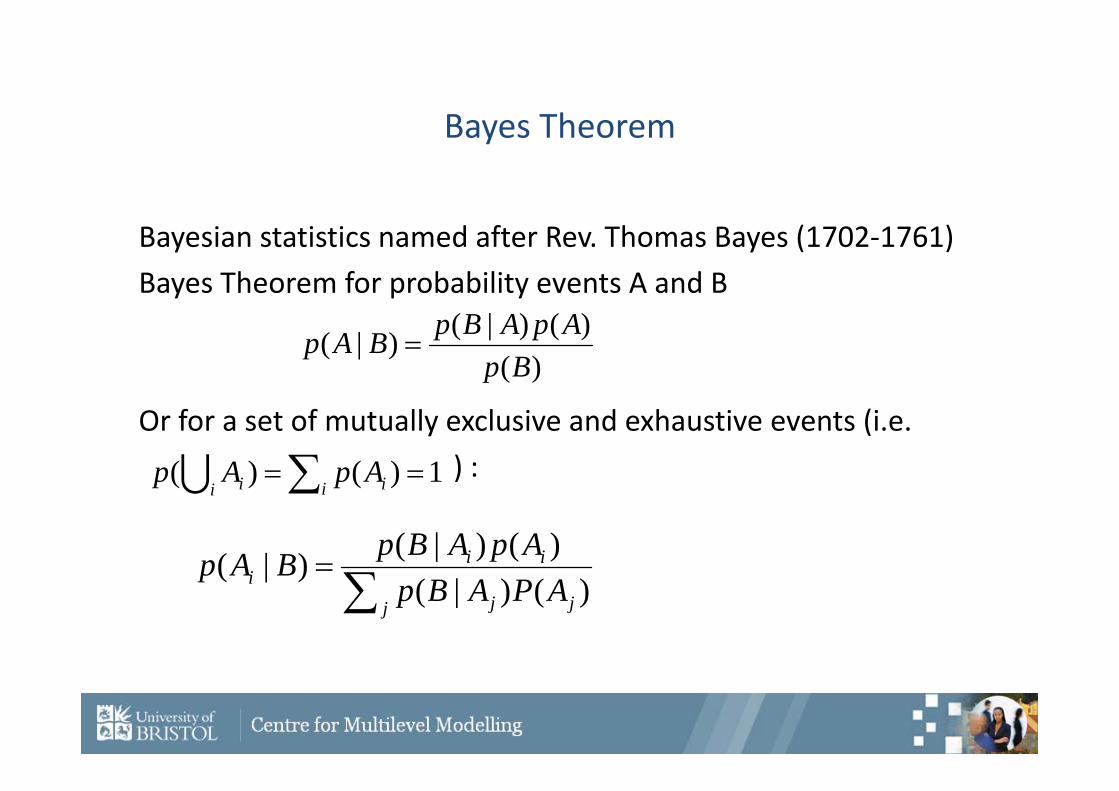
Bayes Theorem
Bayesian statistics named after Rev. Thomas Bayes (1702‐1761)Bayes Theorem for probability events A and B
Or for a set of mutually exclusive and exhaustive events (i.e. ) :
)()()|()|(
BpApABpBAp
i i ii ApAp 1)()(
j jj
iii APABp
ApABpBAp)()|(
)()|()|(
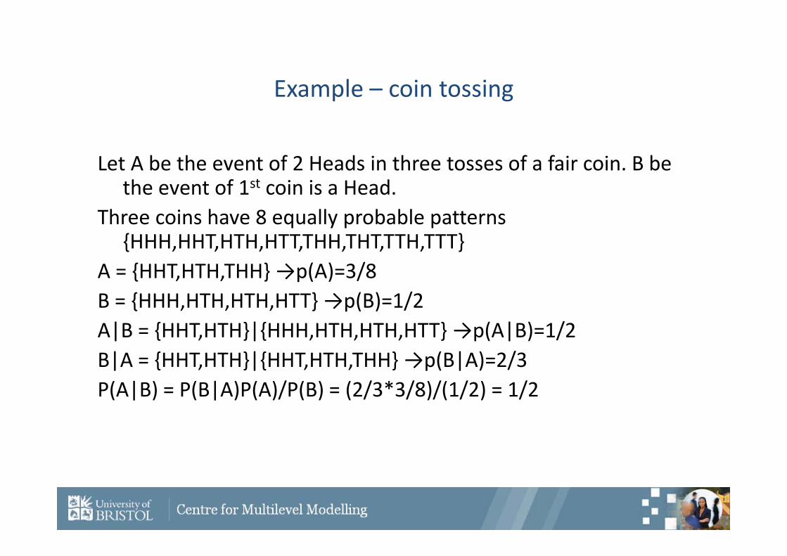
Example – coin tossing
Let A be the event of 2 Heads in three tosses of a fair coin. B be the event of 1st coin is a Head.
Three coins have 8 equally probable patterns {HHH,HHT,HTH,HTT,THH,THT,TTH,TTT}
A = {HHT,HTH,THH} →p(A)=3/8B = {HHH,HTH,HTH,HTT} →p(B)=1/2A|B = {HHT,HTH}|{HHH,HTH,HTH,HTT} →p(A|B)=1/2B|A = {HHT,HTH}|{HHT,HTH,THH} →p(B|A)=2/3P(A|B) = P(B|A)P(A)/P(B) = (2/3*3/8)/(1/2) = 1/2
Example 2 – Diagnostic testing
A new HIV test is claimed to have “95% sensitivity and 98% specificity”
In a population with an HIV prevalence of 1/1000, what is the chance that a patient testing positive actually has HIV?
Let A be the event patient is truly positive, A’ be the event that they are truly negative
Let B be the event that they test positive
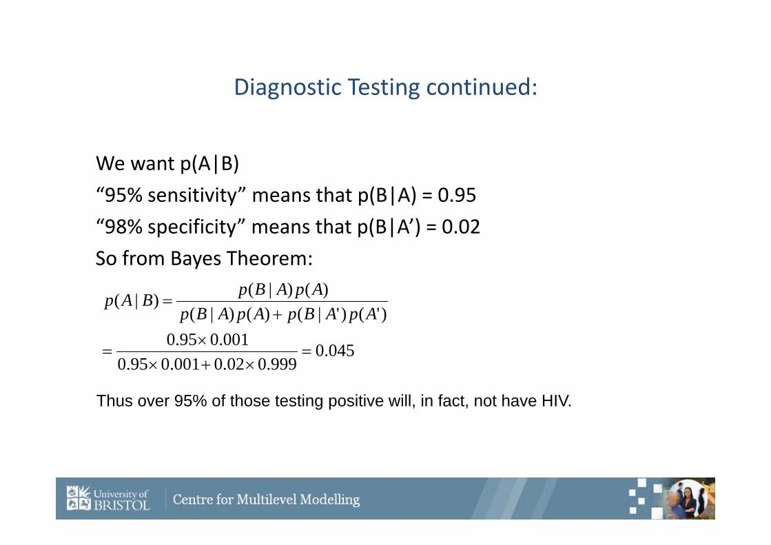
Diagnostic Testing continued:
We want p(A|B)“95% sensitivity” means that p(B|A) = 0.95“98% specificity” means that p(B|A’) = 0.02So from Bayes Theorem:
045.0999.002.0001.095.0
001.095.0)'()'|()()|(
)()|()|(
ApABpApABpApABpBAp
Thus over 95% of those testing positive will, in fact, not have HIV.
Being Bayesian!
So the vital issue in this example is how should this test result change our prior belief that the patient is HIV positive?
The disease prevalence (p=0.001) can be thought of as a ‘prior’ probability.
Observing a positive result causes us to modify this probability to p=0.045 which is our ‘posterior’ probability that the patient is HIV positive.
This use of Bayes theorem applied to observables is uncontroversial however its use in general statistical analyses where parameters are unknown quantities is more controversial.
Bayesian Inference
In Bayesian inference there is a fundamental distinction between• Observable quantities x, i.e. the data• Unknown quantities θθ can be statistical parameters, missing data, latent variables…• Parameters are treated as random variablesIn the Bayesian framework we make probability statements
about model parametersIn the frequentist framework, parameters are fixed non‐random
quantities and the probability statements concern the data.
Prior distributions
As with all statistical analyses we start by positing a model which specifies p(x| θ)
This is the likelihood which relates all variables into a ‘full probability model’
However from a Bayesian point of view :• is unknown so should have a probability distribution
reflecting our uncertainty about it before seeing the data• Therefore we specify a prior distribution p(θ)Note this is like the prevalence in the example
Posterior Distributions
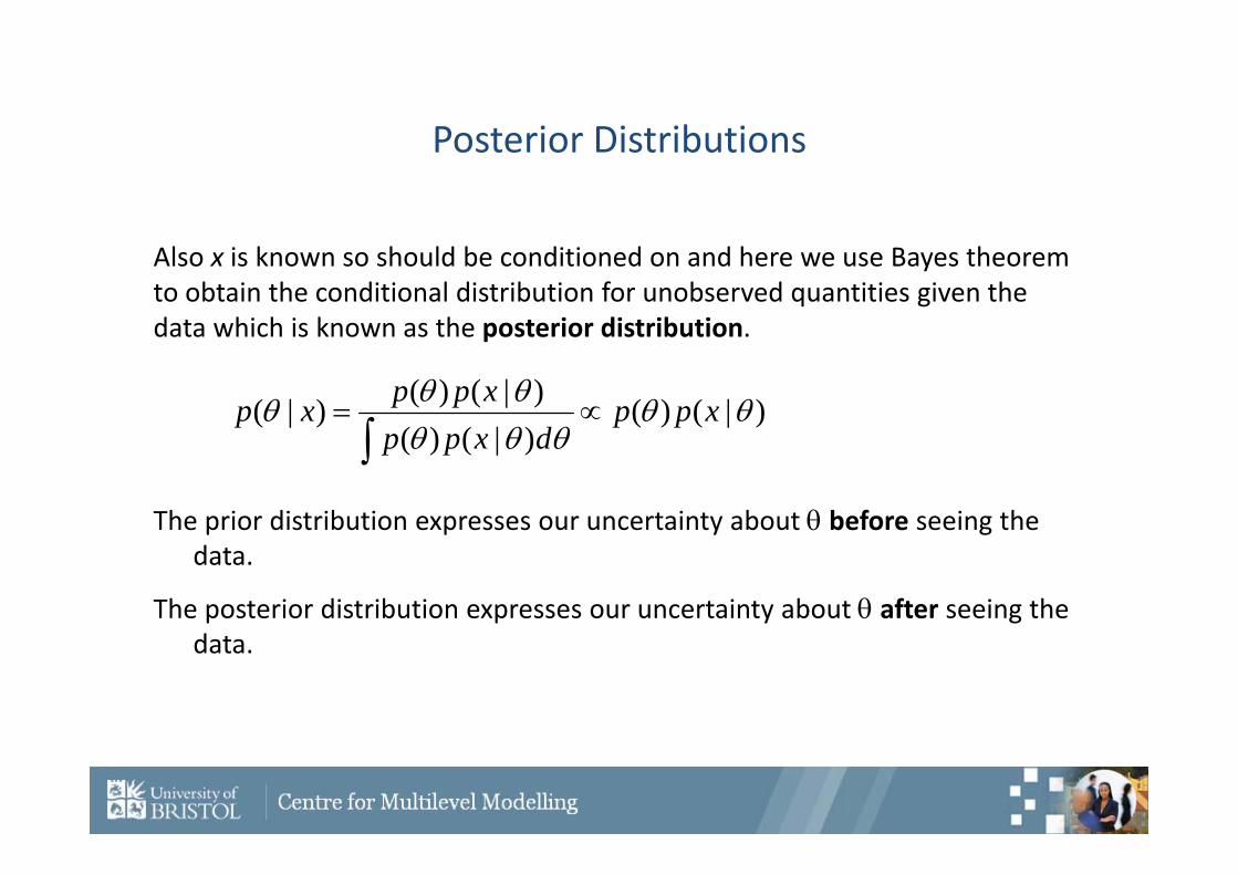
Also x is known so should be conditioned on and here we use Bayes theorem to obtain the conditional distribution for unobserved quantities given the data which is known as the posterior distribution.
The prior distribution expresses our uncertainty about before seeing the data.
The posterior distribution expresses our uncertainty about after seeing the data.
)|()()|()()|()()|(
xppdxpp
xppxp
Examples of Bayesian Inferenceusing the Normal distribution
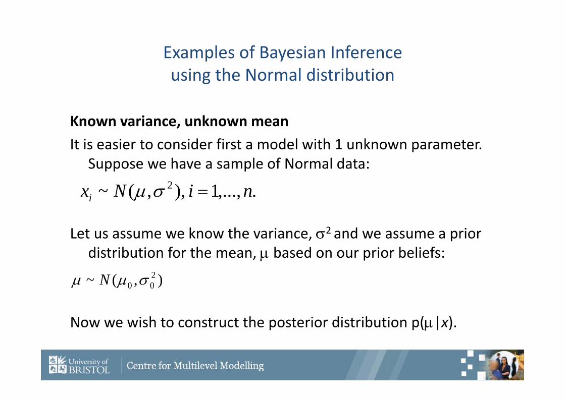
Known variance, unknown meanIt is easier to consider first a model with 1 unknown parameter.
Suppose we have a sample of Normal data:
Let us assume we know the variance, 2 and we assume a prior distribution for the mean, based on our prior beliefs:
Now we wish to construct the posterior distribution p(|x).
.,...,1 ,),(~ 2 niNxi
),(~ 200 N
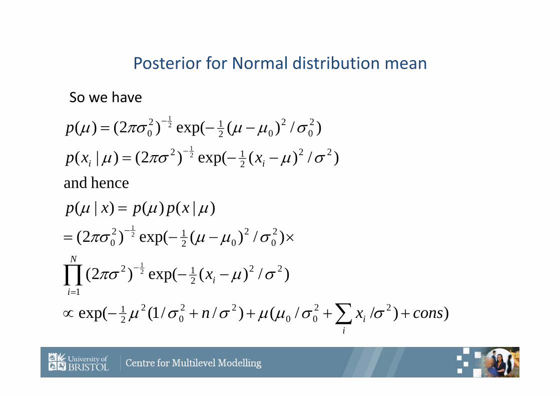
Posterior for Normal distribution mean
So we have
))//()//1(exp(
)/)(exp()2(
)/)(exp()2(
)|()()|(hence and
)/)(exp()2()|(
)/)(exp()2()(
2200
220
221
2
1
2212
20
202
120
22212
20
202
120
21
21
21
21
consxn
x
xppxp
xxp
p
ii
N
ii
ii
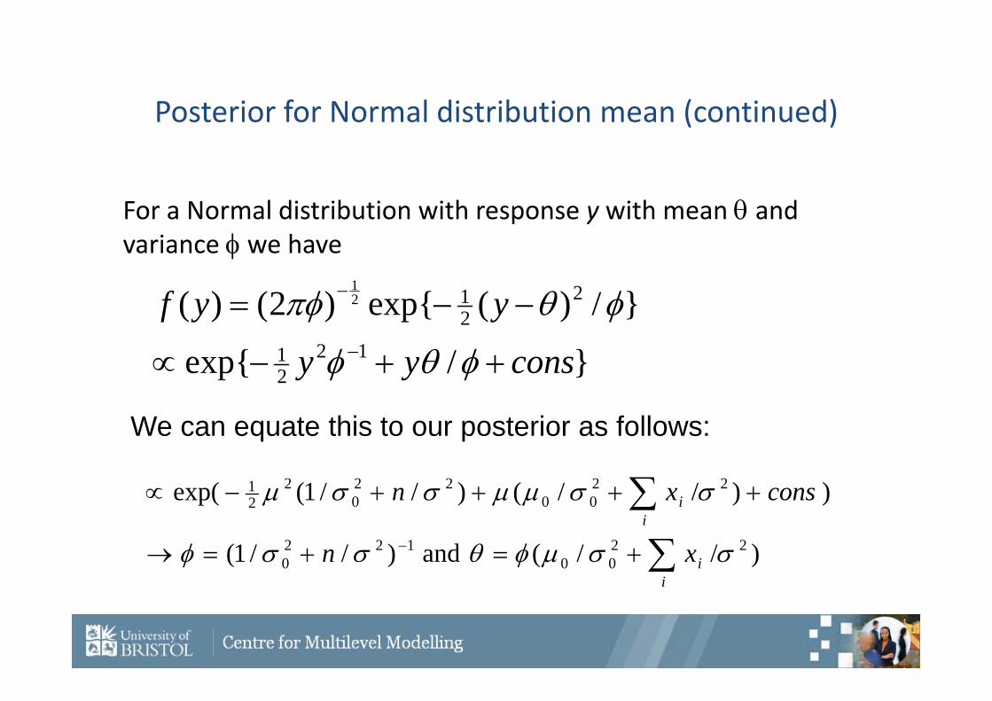
Posterior for Normal distribution mean (continued)
For a Normal distribution with response y with mean and variance we have
}/exp{
}/)(exp{)2()(12
21
2212
1
consyy
yyf
We can equate this to our posterior as follows:
)//( and )//1(
))//()//1(exp(
2200
1220
2200
220
221
ii
ii
xn
consxn
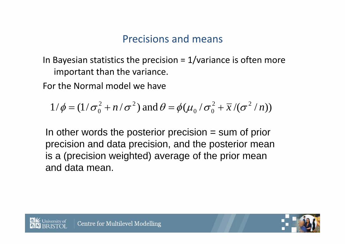
Precisions and means
In Bayesian statistics the precision = 1/variance is often more important than the variance.
For the Normal model we have
))//(/( and )//1(/1 2200
220 nxn
In other words the posterior precision = sum of prior precision and data precision, and the posterior mean is a (precision weighted) average of the prior mean and data mean.
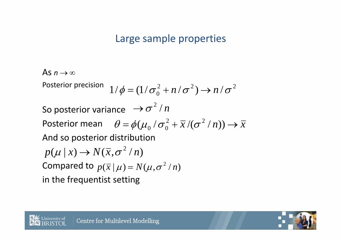
Large sample properties
As nPosterior precision
So posterior variance Posterior mean And so posterior distribution
Compared to in the frequentist setting
2220 / )//1(/1 nn
n/2xnx ))//(/( 22
00
)/,()|( 2 nxNxp )/,()|( 2 nNxp
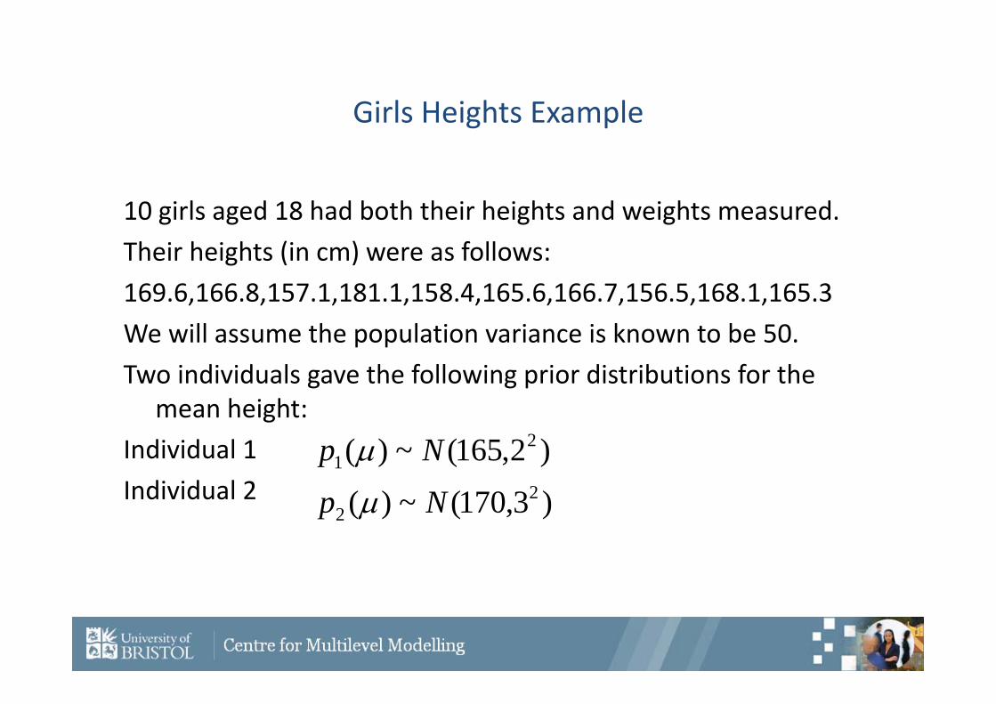
Girls Heights Example
10 girls aged 18 had both their heights and weights measured.Their heights (in cm) were as follows:169.6,166.8,157.1,181.1,158.4,165.6,166.7,156.5,168.1,165.3We will assume the population variance is known to be 50.Two individuals gave the following prior distributions for the
mean height:Individual 1 Individual 2 )3,170(~)(
)2,165(~)(2
2
21
Np
Np
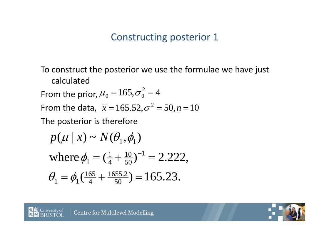
Constructing posterior 1
To construct the posterior we use the formulae we have just calculated
From the prior, From the data,The posterior is therefore
4,165 200
10,50,52.165 2 nx
.23.165)(,222.2)( where
),(~)|(
502.1655
4165
11
15010
41
1
11
Nxp
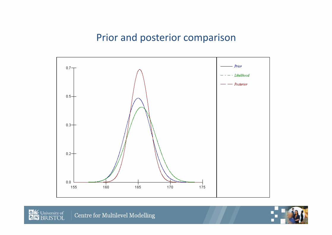
Prior and posterior comparison
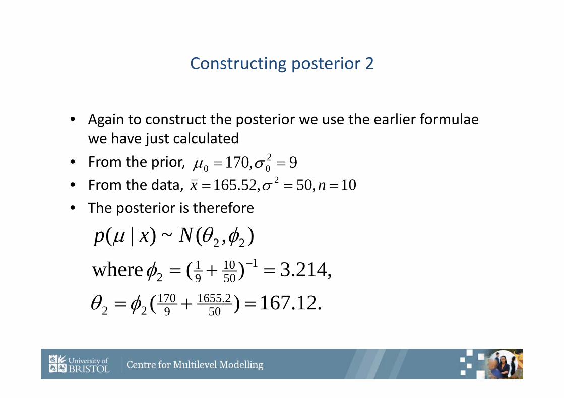
Constructing posterior 2
• Again to construct the posterior we use the earlier formulae we have just calculated
• From the prior, • From the data, • The posterior is therefore
9,170 200
10,50,52.165 2 nx
.12.167)(,214.3)( where
),(~)|(
502.1655
9170
22
15010
91
2
22
Nxp
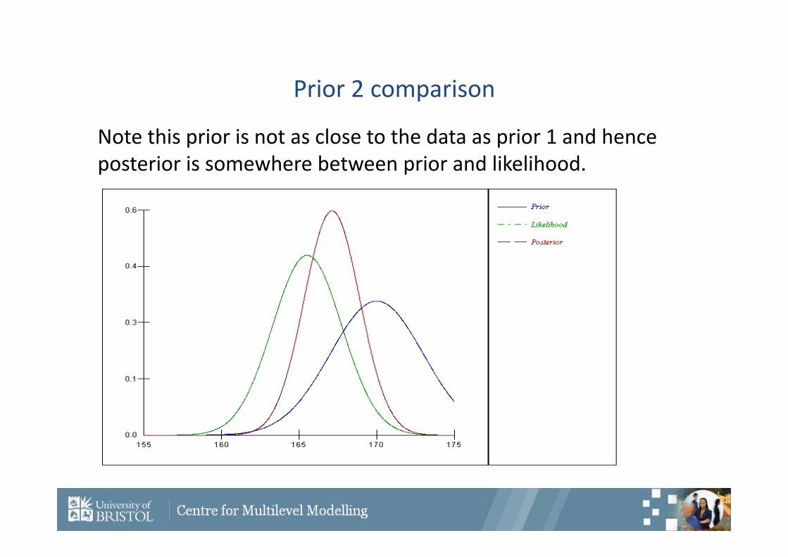
Prior 2 comparison
Note this prior is not as close to the data as prior 1 and hence posterior is somewhere between prior and likelihood.
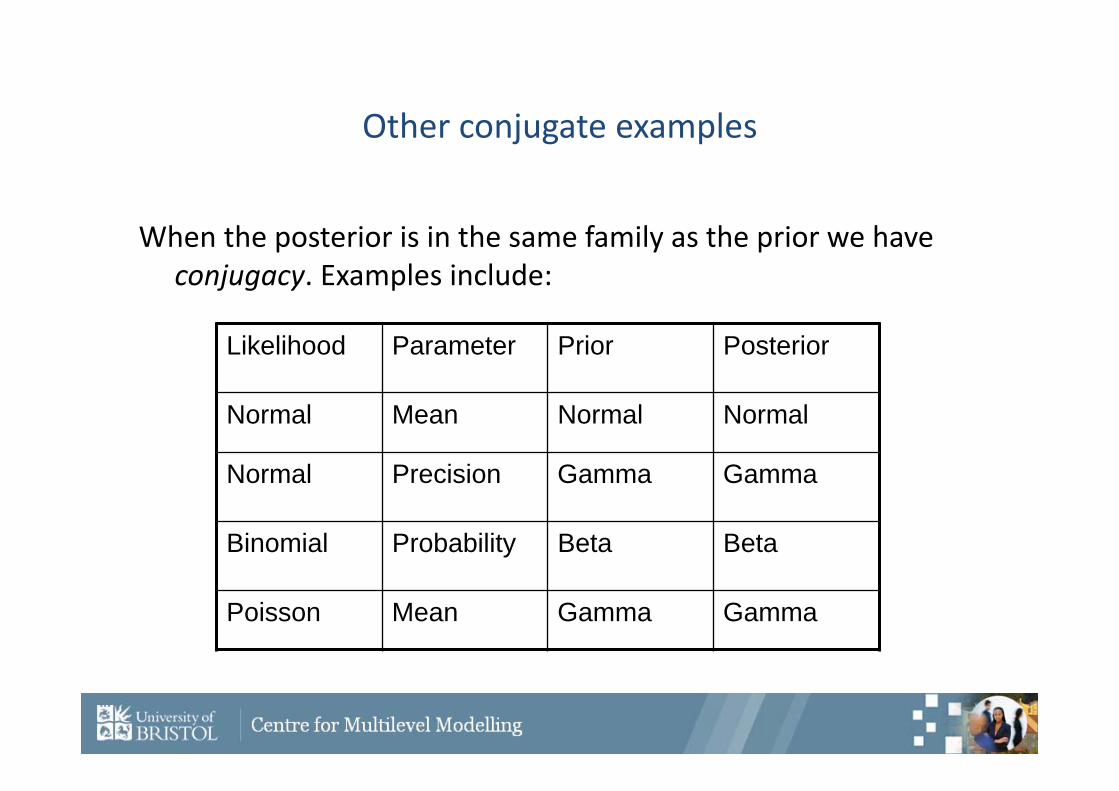
Other conjugate examples
When the posterior is in the same family as the prior we have conjugacy. Examples include:
Likelihood Parameter Prior Posterior
Normal Mean Normal Normal
Normal Precision Gamma Gamma
Binomial Probability Beta Beta
Poisson Mean Gamma Gamma
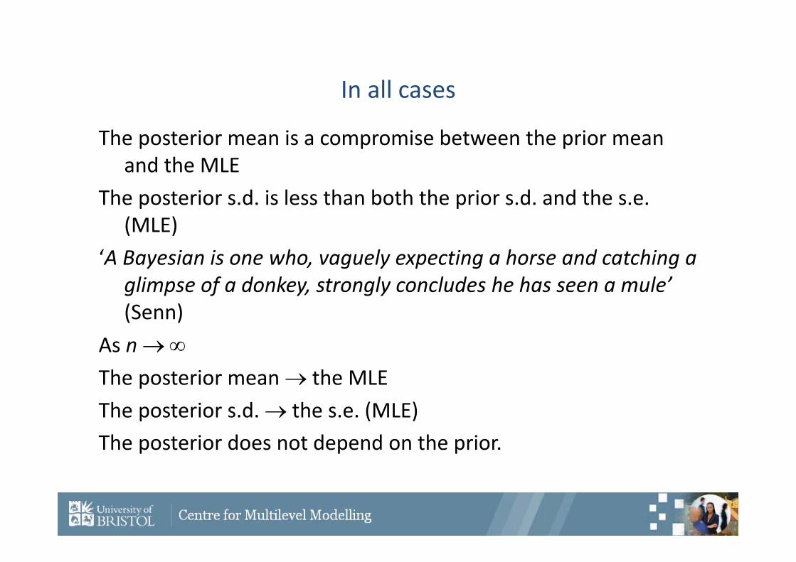
In all cases
The posterior mean is a compromise between the prior mean and the MLE
The posterior s.d. is less than both the prior s.d. and the s.e. (MLE)
‘A Bayesian is one who, vaguely expecting a horse and catching a glimpse of a donkey, strongly concludes he has seen a mule’(Senn)
As nThe posterior mean the MLEThe posterior s.d. the s.e. (MLE)The posterior does not depend on the prior.
Non‐informative priors
We often do not have any prior information, although true Bayesian’s would argue we always have some prior information!
We would hope to have good agreement between the frequentist approach and the Bayesian approach with a non‐informative prior.
Diffuse or flat priors are often better terms to use as no prior is strictly non‐informative!
For our example of an unknown mean, candidate priors are a Uniform distribution over a large range or a Normal distribution with a huge variance.
Point and Interval Estimation
In Bayesian inference the outcome of interest for a parameter is its full posterior distribution however we may be interested in summaries of this distribution.
A simple point estimate would be the mean of the posterior. (although the median and mode are alternatives.)
Interval estimates are also easy to obtain from the posterior distribution and are given several names, for example credible intervals, Bayesian confidence intervals and Highest density regions (HDR). All of these refer to the same quantity.
Credible Intervals
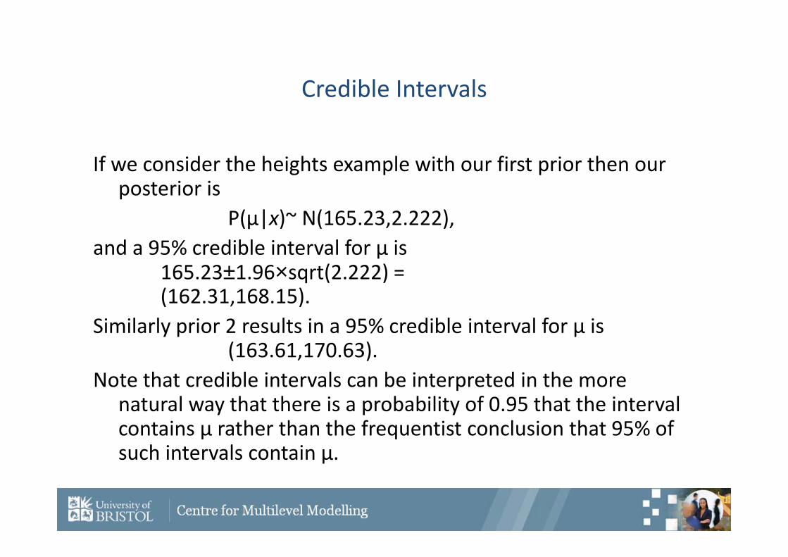
If we consider the heights example with our first prior then our posterior is
P(μ|x)~ N(165.23,2.222),and a 95% credible interval for μ is
165.23±1.96×sqrt(2.222) = (162.31,168.15).
Similarly prior 2 results in a 95% credible interval for μ is (163.61,170.63).
Note that credible intervals can be interpreted in the more natural way that there is a probability of 0.95 that the interval contains μ rather than the frequentist conclusion that 95% of such intervals contain μ.
MCMC METHODS
How does one fit models in a Bayesian framework?
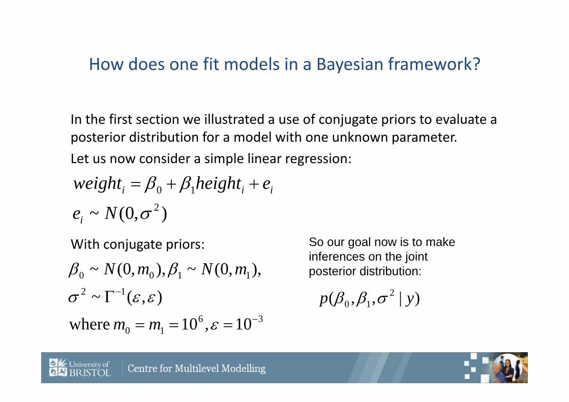
In the first section we illustrated a use of conjugate priors to evaluate a posterior distribution for a model with one unknown parameter.Let us now consider a simple linear regression:
With conjugate priors:
),0(~ 210
Ne
eheightweight
i
iii
3610
121100
10,10 where),(~
),,0(~),,0(~
mm
mNmN
So our goal now is to make inferences on the joint posterior distribution:
)|,,( 210 yp
MCMC Methods
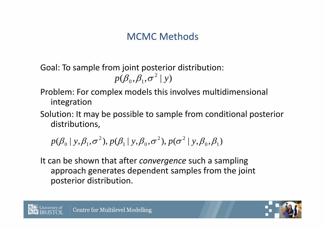
Goal: To sample from joint posterior distribution:
Problem: For complex models this involves multidimensional integration
Solution: It may be possible to sample from conditional posterior distributions,
It can be shown that after convergence such a sampling approach generates dependent samples from the joint posterior distribution.
)|,,( 210 yp
),,|(),,,|(),,,|( 1022
012
10 ypypyp
Gibbs Sampling
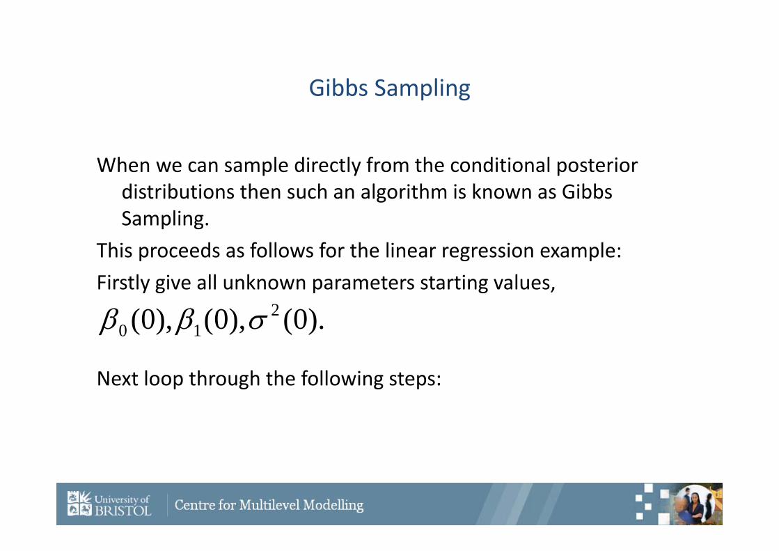
When we can sample directly from the conditional posterior distributions then such an algorithm is known as Gibbs Sampling.
This proceeds as follows for the linear regression example:Firstly give all unknown parameters starting values,
Next loop through the following steps:
).0(),0(),0( 210
Gibbs Sampling ctd.
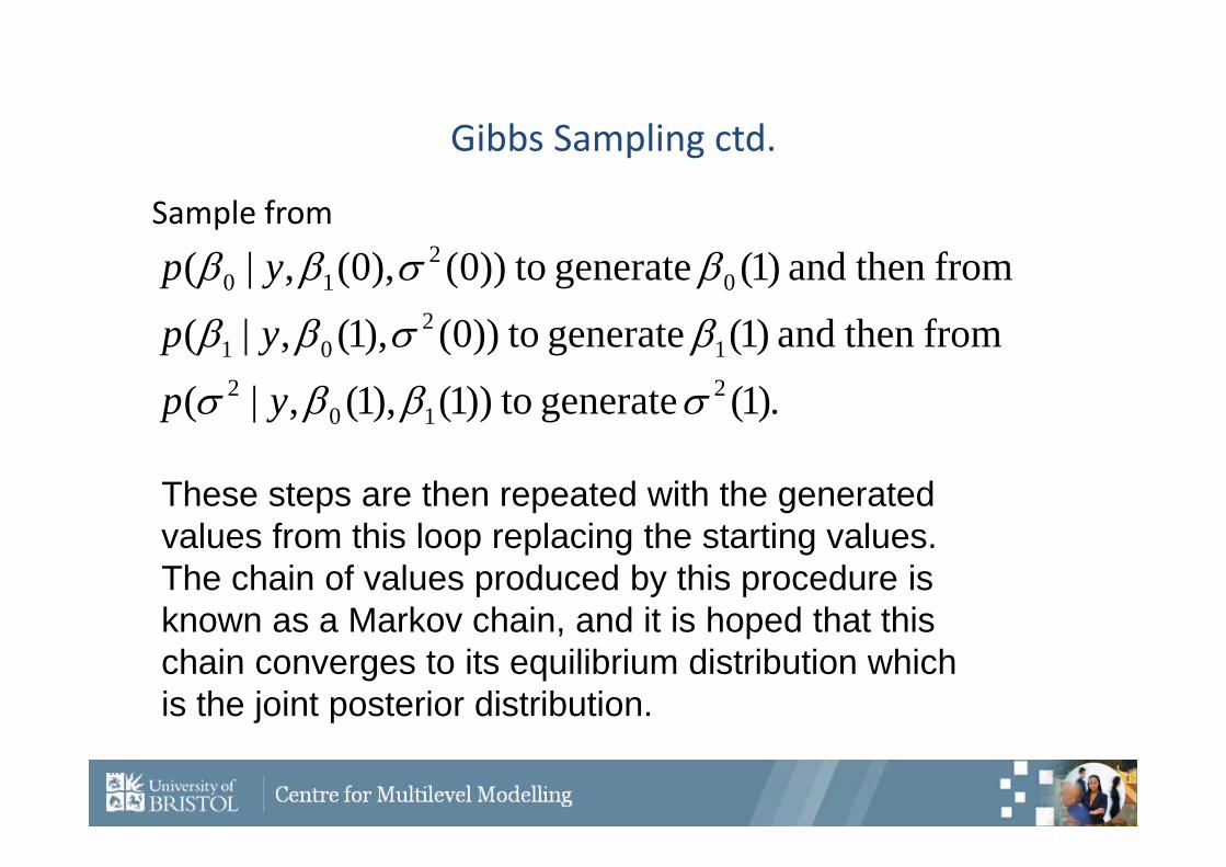
Sample from
.)1( generate to))1(),1(,|(
from then and )1( generate to))0(),1(,|(
from then and )1( generate to))0(),0(,|(
210
21
201
02
10
yp
yp
yp
These steps are then repeated with the generatedvalues from this loop replacing the starting values.The chain of values produced by this procedure isknown as a Markov chain, and it is hoped that thischain converges to its equilibrium distribution whichis the joint posterior distribution.
Calculating the conditional distributions
In order for the algorithm to work we need to sample from the conditional posterior distributions.
If these distributions have standard forms then it is easy to draw random samples from them.
Mathematically we write down the full posterior and assume all parameters are constants apart from the parameter of interest.
We then try to match the resulting formulae to a standard distribution.
The next 4 slides will probably be skipped but are in the talk for reference purposes
Note the new STAT‐JR software gives these derivations!
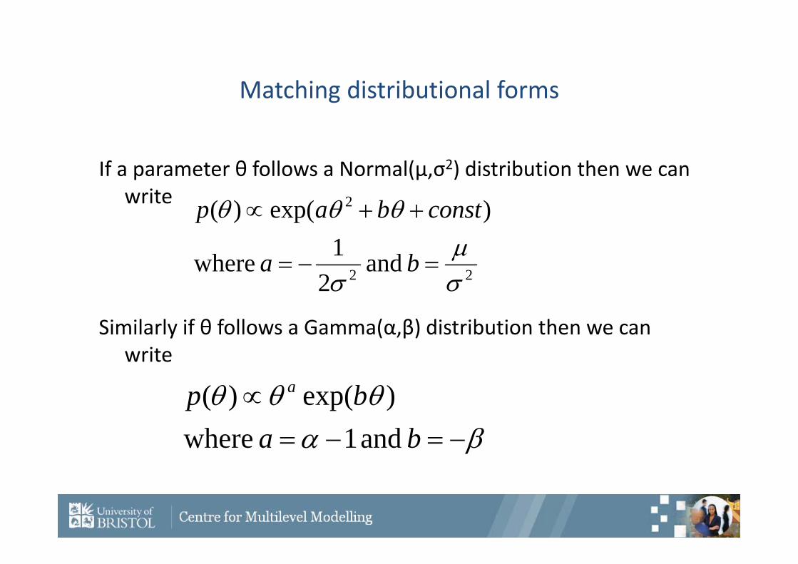
Matching distributional forms
If a parameter θ follows a Normal(μ,σ2) distribution then we can write
Similarly if θ follows a Gamma(α,β) distribution then we can write
22
2
and 2
1 where
)exp()(
ba
constbap
babp a
and 1 where )exp()(
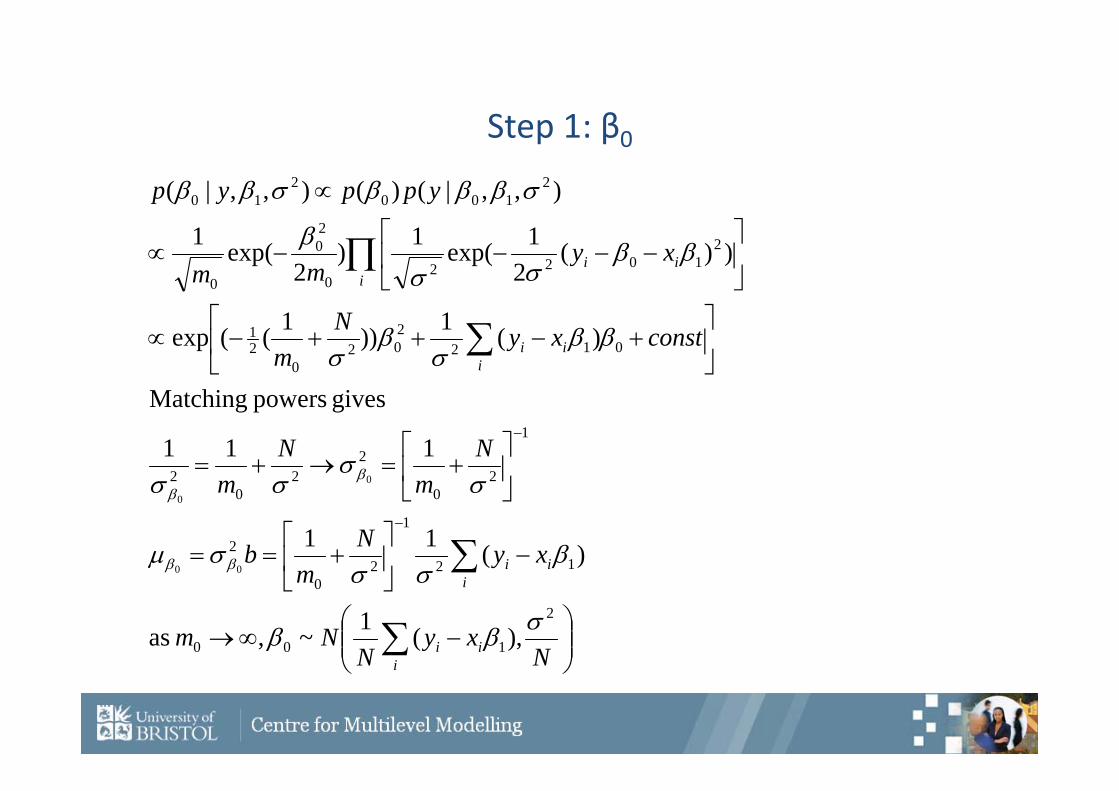
Step 1: β0
Nxy
NNm
xyNm
b
Nm
Nm
constxyNm
xymm
yppyp
iii
iii
iii
iii
2
100
12
1
20
2
1
20
22
02
012202
021
21022
0
20
0
2100
210
,)(1~, as
)(11
111
gives powers Matching
)(1))1((exp
))(2
1exp(1)2
exp(1
),,|()(),,|(
00
0
0
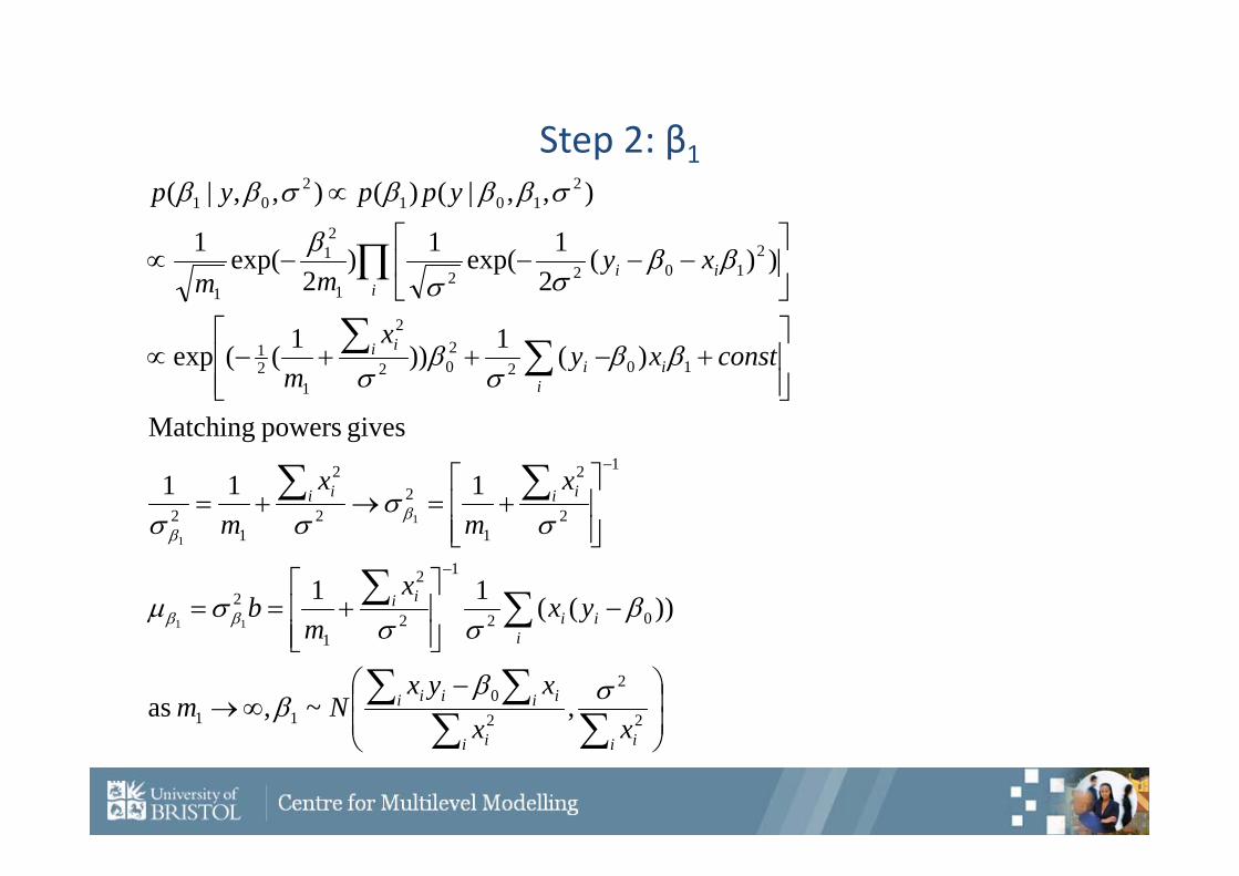
Step 2: β1
i ii i
i ii ii
iii
i i
i ii i
ii
ii i
iii
xxxyx
Nm
yxx
mb
xm
xm
constxyx
m
xymm
yppyp
2
2
20
11
02
1
2
2
1
2
1
2
2
1
22
2
12
102202
2
121
21022
1
21
1
2101
201
,~, as
))((11
111
gives powers Matching
)(1))1((exp
))(2
1exp(1)2
exp(1
),,|()(),,|(
11
1
1
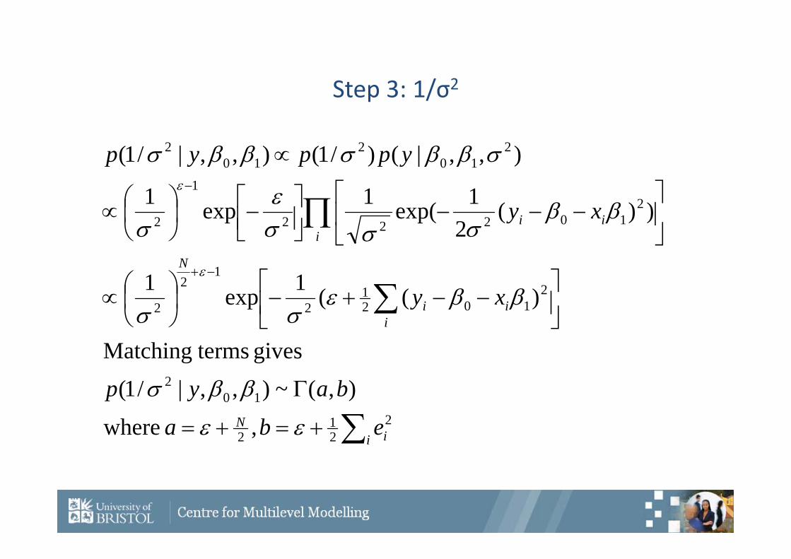
Step 3: 1/σ2
i iN
iii
N
iii
eba
bayp
xy
xy
yppyp
221
2
102
2102
12
12
2
210222
1
2
210
210
2
, where
),(~),,|/1(gives termsMatching
)((1exp1
))(2
1exp(1exp1
),,|()/1(),,|/1(
Algorithm Summary
Repeat the following three steps1. Generate β0 from its Normal conditional distribution.2. Generate β1 from its Normal conditional distribution.3. Generate 1/σ2 from its Gamma conditional distributionConvergence and burn‐inTwo questions that immediately spring to mind are:1. We start from arbitrary starting values so when can we
safely say that our samples are from the correct distribution?
2. After this point how long should we run the chain for and store values?
MCMC DIAGNOSTICS
Checking Convergence
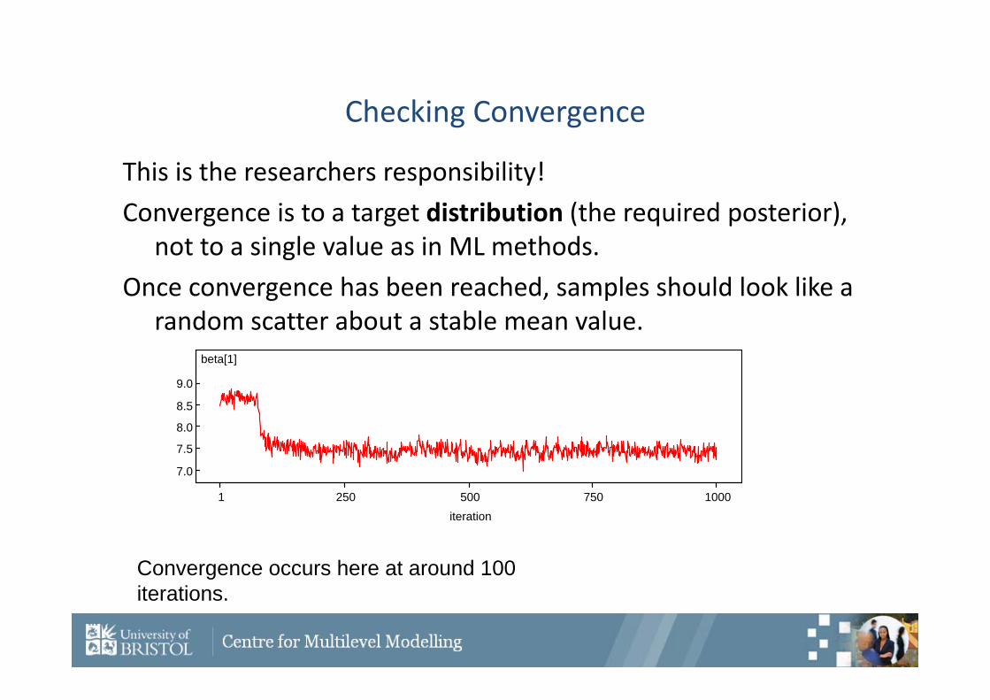
This is the researchers responsibility!Convergence is to a target distribution (the required posterior),
not to a single value as in ML methods.Once convergence has been reached, samples should look like a
random scatter about a stable mean value.beta[1]
iteration1 250 500 750 1000
7.0
7.5
8.0
8.5
9.0
Convergence occurs here at around 100 iterations.
How many iterations after convergence?
After convergence, further iterations are needed to obtain samples for posterior inference.
More iterations = more accurate posterior estimates.MCMC chains are dependent samples and so the dependence or autocorrelation in the chain will influence how many iterations we need.
Accuracy of the posterior estimates can be assessed by the Monte Carlo standard error (MCSE) for each parameter.
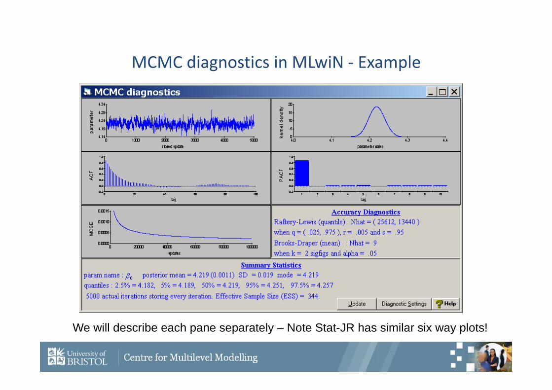
MCMC diagnostics in MLwiN ‐ Example
We will describe each pane separately – Note Stat-JR has similar six way plots!
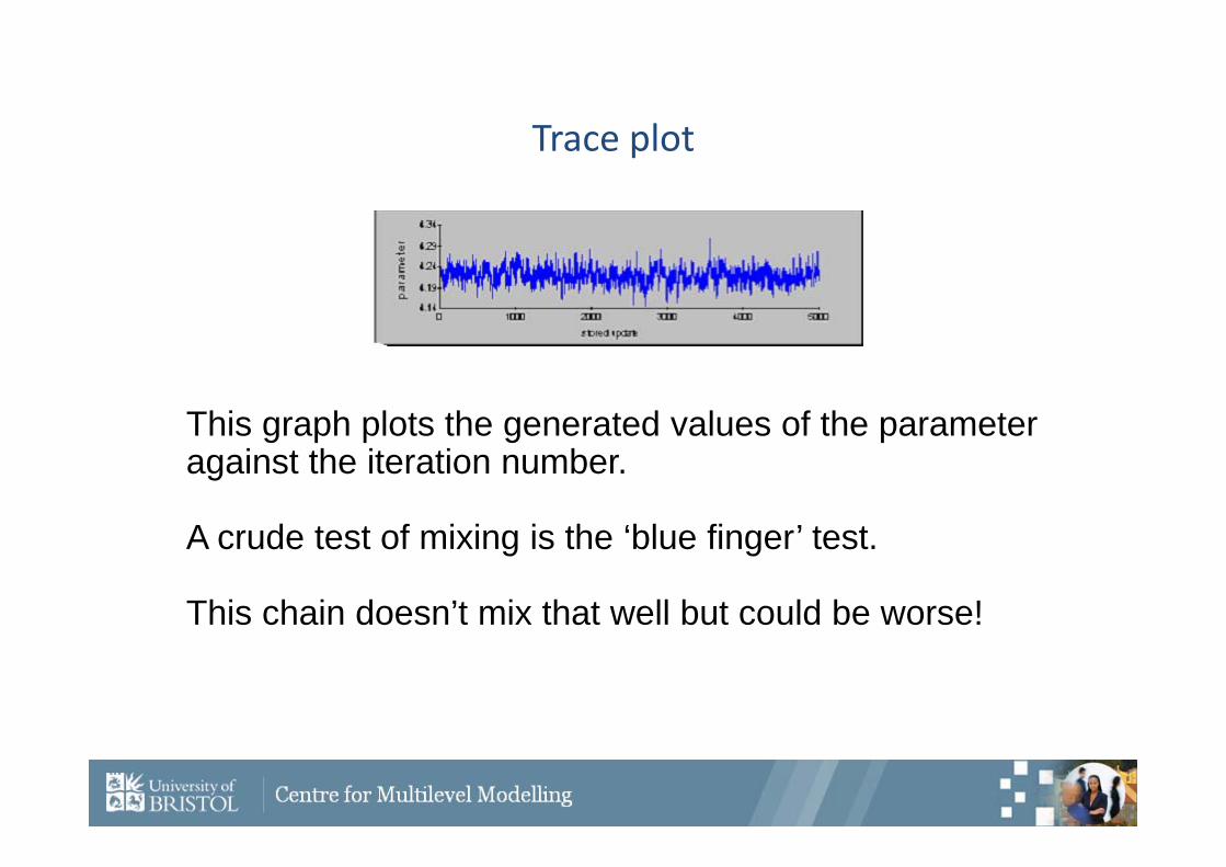
Trace plot
This graph plots the generated values of the parameter against the iteration number.
A crude test of mixing is the ‘blue finger’ test.
This chain doesn’t mix that well but could be worse!
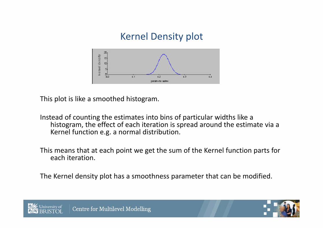
Kernel Density plot
This plot is like a smoothed histogram.
Instead of counting the estimates into bins of particular widths like a histogram, the effect of each iteration is spread around the estimate via a Kernel function e.g. a normal distribution.
This means that at each point we get the sum of the Kernel function parts for each iteration.
The Kernel density plot has a smoothness parameter that can be modified.
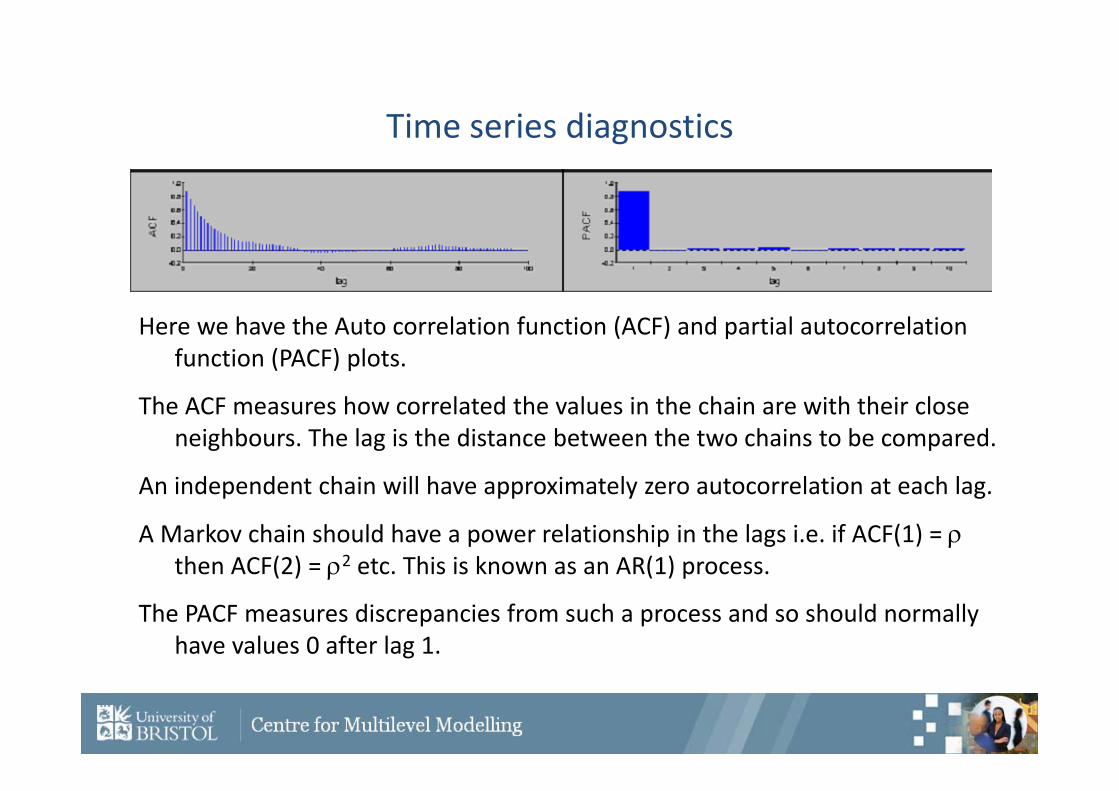
Time series diagnostics
Here we have the Auto correlation function (ACF) and partial autocorrelation function (PACF) plots.
The ACF measures how correlated the values in the chain are with their close neighbours. The lag is the distance between the two chains to be compared.
An independent chain will have approximately zero autocorrelation at each lag.
A Markov chain should have a power relationship in the lags i.e. if ACF(1) = then ACF(2) = 2 etc. This is known as an AR(1) process.
The PACF measures discrepancies from such a process and so should normally have values 0 after lag 1.
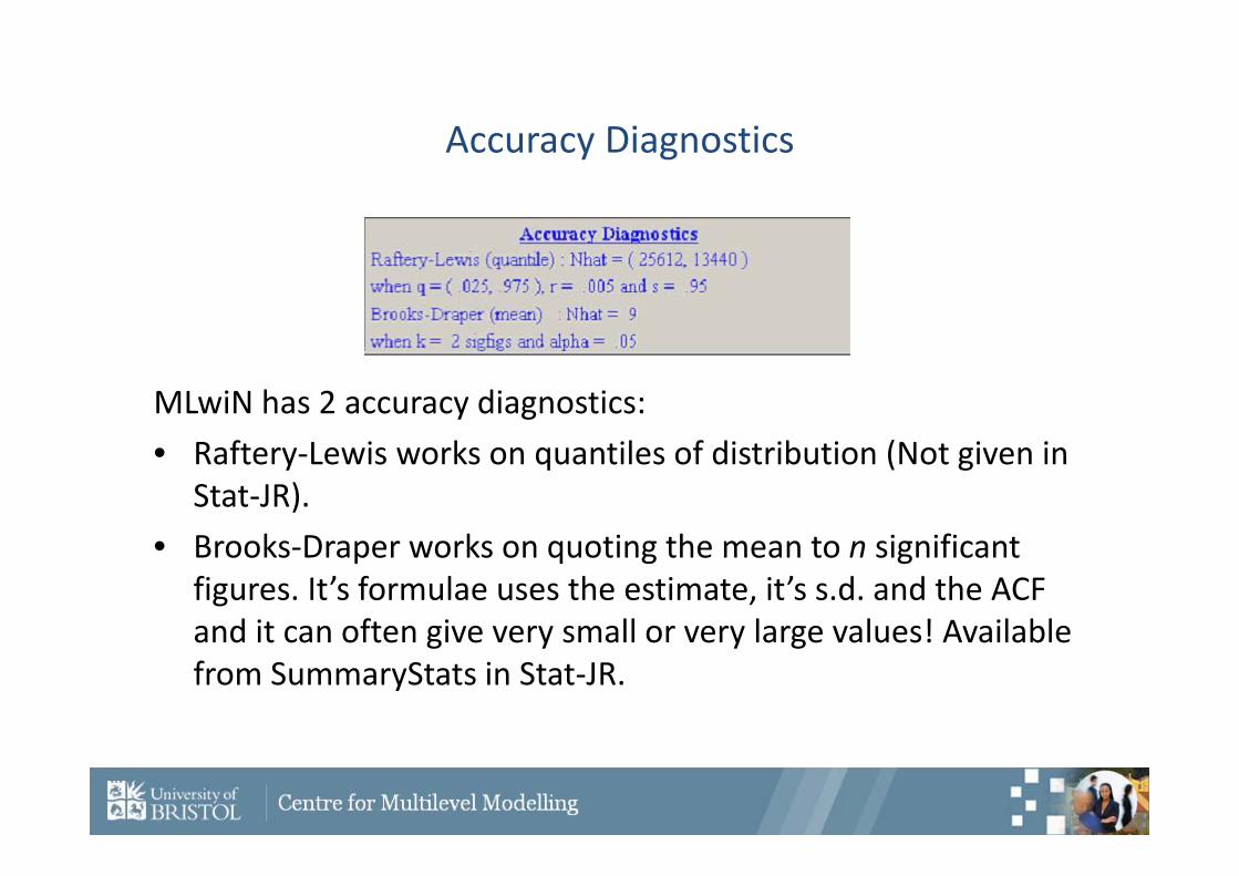
Accuracy Diagnostics
MLwiN has 2 accuracy diagnostics:• Raftery‐Lewis works on quantiles of distribution (Not given in
Stat‐JR).• Brooks‐Draper works on quoting the mean to n significant
figures. It’s formulae uses the estimate, it’s s.d. and the ACF and it can often give very small or very large values! Available from SummaryStats in Stat‐JR.
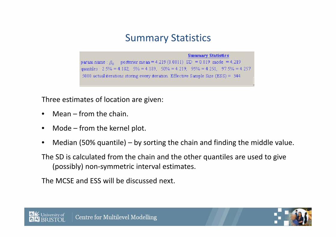
Summary Statistics
Three estimates of location are given:
• Mean – from the chain.
• Mode – from the kernel plot.
• Median (50% quantile) – by sorting the chain and finding the middle value.
The SD is calculated from the chain and the other quantiles are used to give (possibly) non‐symmetric interval estimates.
The MCSE and ESS will be discussed next.
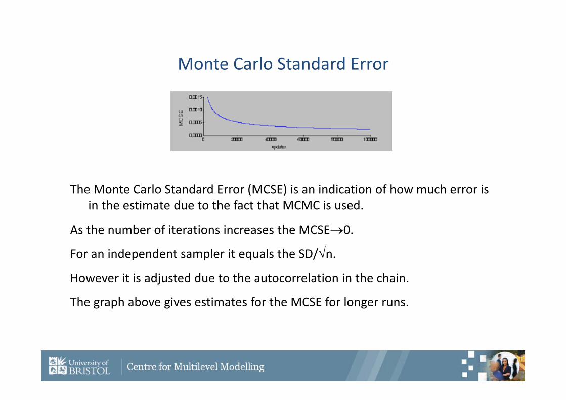
Monte Carlo Standard Error
The Monte Carlo Standard Error (MCSE) is an indication of how much error is in the estimate due to the fact that MCMC is used.
As the number of iterations increases the MCSE0.
For an independent sampler it equals the SD/n.
However it is adjusted due to the autocorrelation in the chain.
The graph above gives estimates for the MCSE for longer runs.
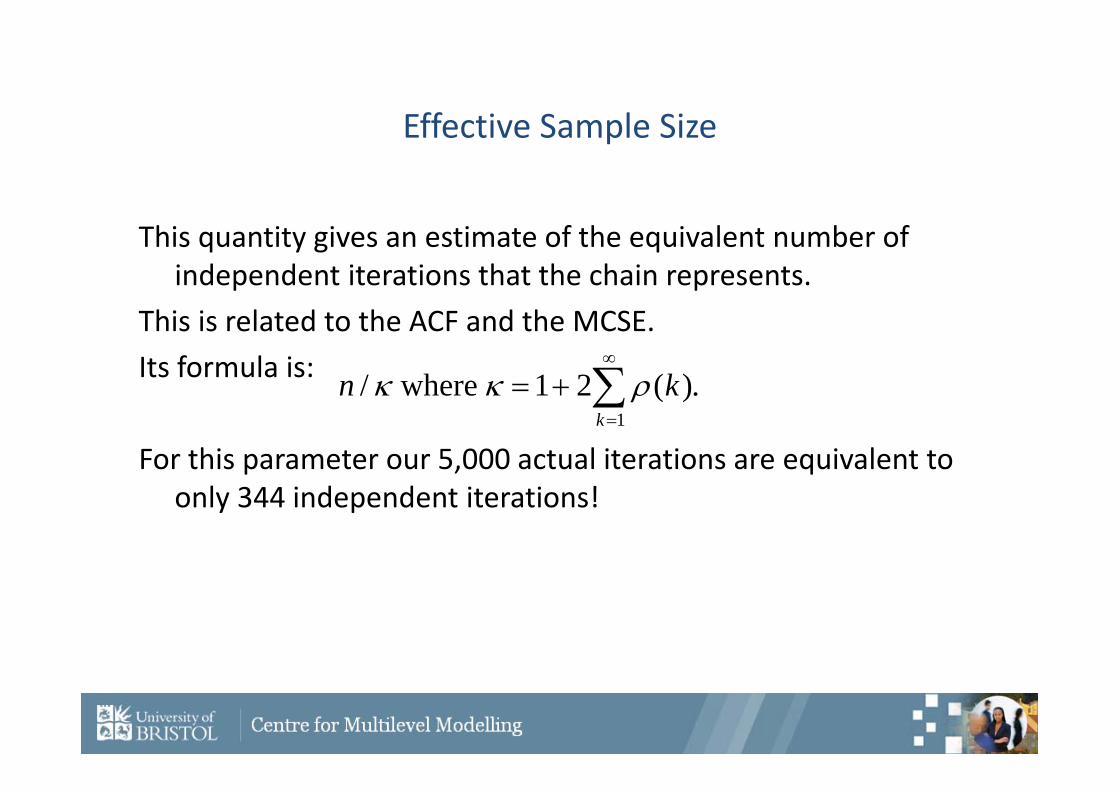
Effective Sample Size
This quantity gives an estimate of the equivalent number of independent iterations that the chain represents.
This is related to the ACF and the MCSE.Its formula is:
For this parameter our 5,000 actual iterations are equivalent to only 344 independent iterations!
.)(21 where/1
k
kn
Inference using posterior samples from MCMC runs
A powerful feature of MCMC and the Bayesian approach is that all inference is based on the joint posterior distribution.
We can therefore address a wide range of substantive questions by appropriate summaries of the posterior.
Typically report either the mean or median of the posterior samples for each parameter of interest as a point estimate
2.5% and 97.5% percentiles of the posterior sample for each parameter give a 95% posterior credible interval (interval within which the parameter lies with probability 0.95)
Derived Quantities
Once we have a sample from the posterior we can answer lots of questions simply by investigating this sample.
Examples:What is the probability that θ>0? What is the probability that θ1> θ2?What is a 95% interval for θ1/(θ1+ θ2)?
MODEL COMPARISON
Model Comparison in MCMC
In frequentist statistics there are many options including:• Likelihood ratio (deviance) tests• Wald Tests• Information Criterion – e.g. AIC/BICHere we look at a criterion that can be used with MCMC and
which for a linear regression model is equivalent to the AIC –the Deviance information criterion (DIC).
DIC
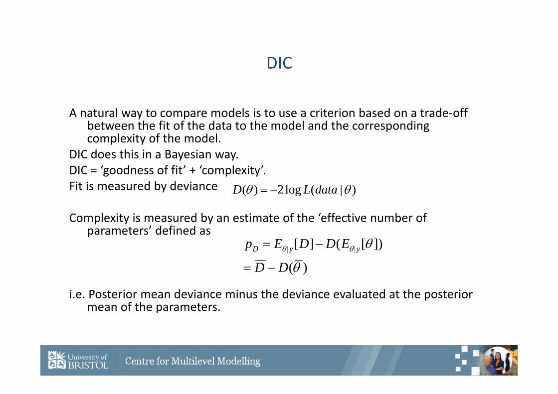
A natural way to compare models is to use a criterion based on a trade‐off between the fit of the data to the model and the corresponding complexity of the model.
DIC does this in a Bayesian way.DIC = ‘goodness of fit’ + ‘complexity’.Fit is measured by deviance
Complexity is measured by an estimate of the ‘effective number of parameters’ defined as
i.e. Posterior mean deviance minus the deviance evaluated at the posterior mean of the parameters.
)|(log2)( dataLD
)(
])[(][ ||
DD
EDDEp yyD
DIC (continued)
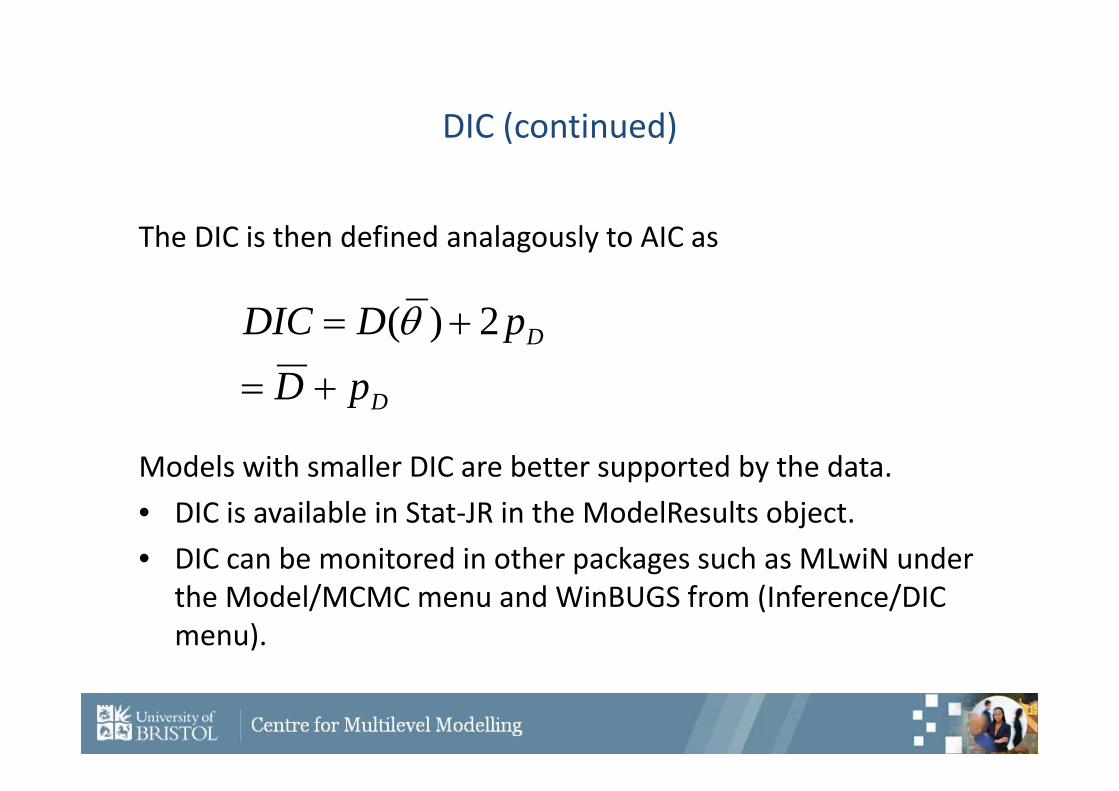
The DIC is then defined analagously to AIC as
Models with smaller DIC are better supported by the data.• DIC is available in Stat‐JR in the ModelResults object.• DIC can be monitored in other packages such as MLwiN under
the Model/MCMC menu and WinBUGS from (Inference/DIC menu).
D
D
pDpDDIC
2)(
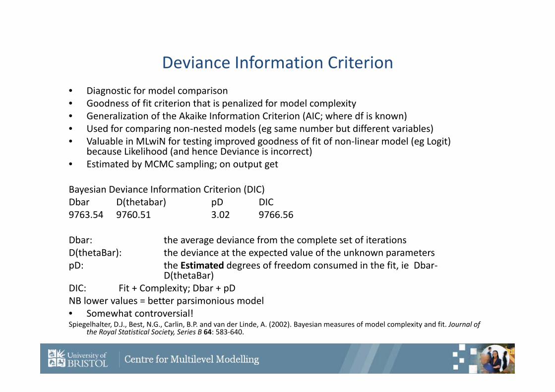
Deviance Information Criterion• Diagnostic for model comparison• Goodness of fit criterion that is penalized for model complexity• Generalization of the Akaike Information Criterion (AIC; where df is known)• Used for comparing non‐nested models (eg same number but different variables)• Valuable in MLwiN for testing improved goodness of fit of non‐linear model (eg Logit)
because Likelihood (and hence Deviance is incorrect)• Estimated by MCMC sampling; on output get
Bayesian Deviance Information Criterion (DIC)Dbar D(thetabar) pD DIC9763.54 9760.51 3.02 9766.56
Dbar: the average deviance from the complete set of iterationsD(thetaBar): the deviance at the expected value of the unknown parameters pD: the Estimated degrees of freedom consumed in the fit, ie Dbar‐
D(thetaBar) DIC: Fit + Complexity; Dbar + pDNB lower values = better parsimonious model• Somewhat controversial! Spiegelhalter, D.J., Best, N.G., Carlin, B.P. and van der Linde, A. (2002). Bayesian measures of model complexity and fit. Journal of
the Royal Statistical Society, Series B 64: 583‐640.
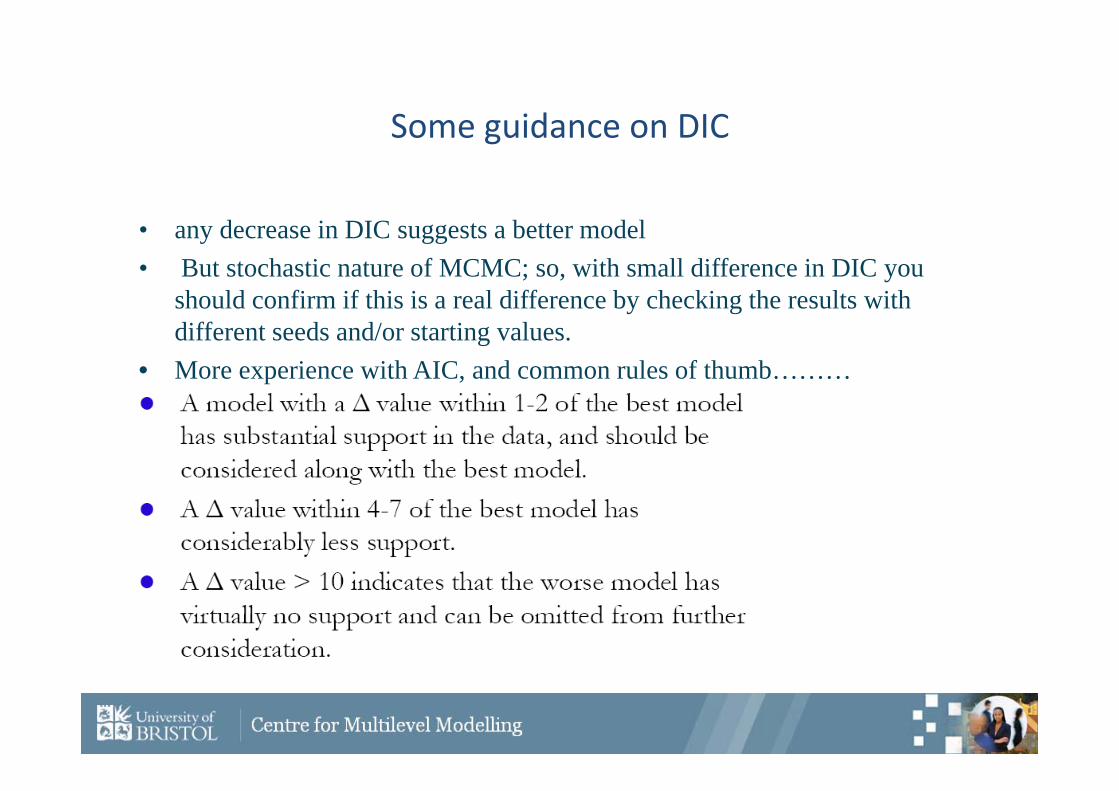
Some guidance on DIC
• any decrease in DIC suggests a better model• But stochastic nature of MCMC; so, with small difference in DIC you
should confirm if this is a real difference by checking the results with different seeds and/or starting values.
• More experience with AIC, and common rules of thumb………
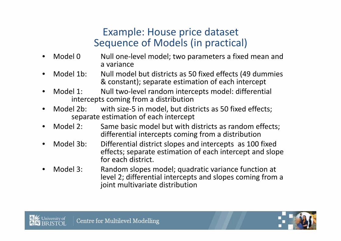
Example: House price datasetSequence of Models (in practical)
• Model 0 Null one‐level model; two parameters a fixed mean and a variance
• Model 1b: Null model but districts as 50 fixed effects (49 dummies & constant); separate estimation of each intercept
• Model 1: Null two‐level random intercepts model: differential intercepts coming from a distribution
• Model 2b: with size‐5 in model, but districts as 50 fixed effects; separate estimation of each intercept
• Model 2: Same basic model but with districts as random effects; differential intercepts coming from a distribution
• Model 3b: Differential district slopes and intercepts as 100 fixed effects; separate estimation of each intercept and slope for each district.
• Model 3: Random slopes model; quadratic variance function at level 2; differential intercepts and slopes coming from a joint multivariate distribution
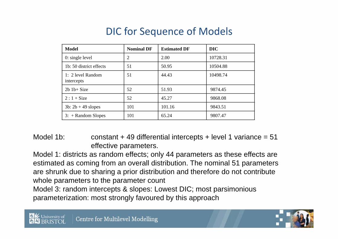
DIC for Sequence of ModelsModel Nominal DF Estimated DF DIC
0: single level 2 2.00 10728.31
1b: 50 district effects 51 50.95 10504.88
1: 2 level Random intercepts
51 44.43 10498.74
2b 1b+ Size 52 51.93 9874.45
2 : 1 + Size 52 45.27 9868.08
3b: 2b + 49 slopes 101 101.16 9843.51
3: + Random Slopes 101 65.24 9807.47
Model 1b: constant + 49 differential intercepts + level 1 variance = 51 effective parameters.
Model 1: districts as random effects; only 44 parameters as these effects are estimated as coming from an overall distribution. The nominal 51 parameters are shrunk due to sharing a prior distribution and therefore do not contribute whole parameters to the parameter countModel 3: random intercepts & slopes: Lowest DIC; most parsimonious parameterization: most strongly favoured by this approach
SUMMARY & COMPARISON WITH FREQUENTIST APPROACH
Markov chain Monte Carlo (MCMC)
• MCMC methods are Bayesian estimation techniques which can be used to estimate multilevel models
• MCMC works by drawing a random sample of values for each parameter from its probability distribution
• The mean and standard deviation of each random sample gives the point estimate and standard error for that parameter
Estimating a model using MCMC estimation
• We start by specifying the model and our prior knowledge for each parameter (nearly always no knowledge!)
• Next we specify initial values for the model parameters (nearly always the IGLS estimates)
• We then run the MCMC algorithm and obtain the parameter chains
• We discard the initial burn‐in iterations when the chains are settling down (converging to their posterior distributions)
• Summary statistics for the remaining monitoring iterationsare then calculated:– Point estimates and standard errors are given by the means and standard deviations of the chains
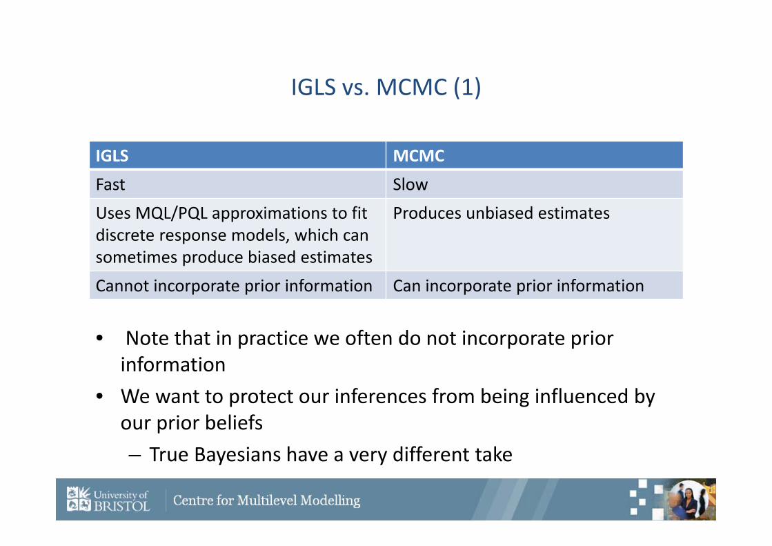
IGLS vs. MCMC (1)
• Note that in practice we often do not incorporate prior information
• We want to protect our inferences from being influenced by our prior beliefs– True Bayesians have a very different take
IGLS MCMCFast SlowUses MQL/PQL approximations to fit discrete response models, which can sometimes produce biased estimates
Produces unbiased estimates
Cannot incorporate prior information Can incorporate prior information
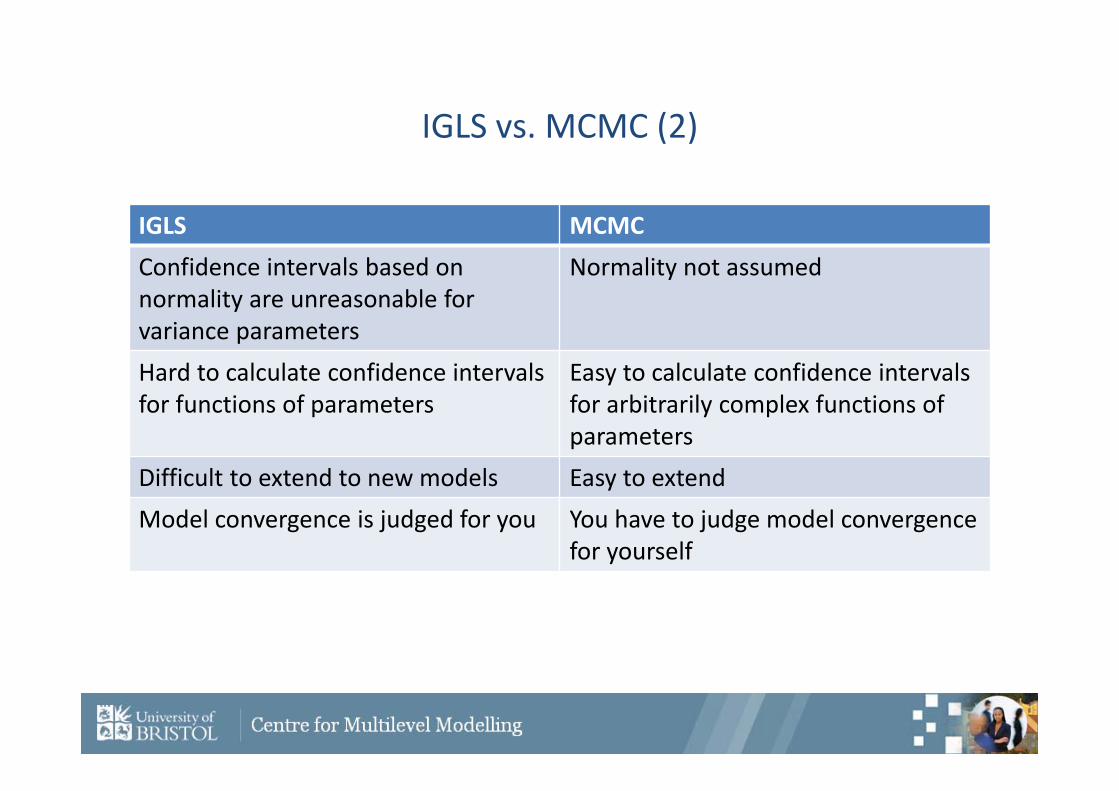
IGLS vs. MCMC (2)
IGLS MCMCConfidence intervals based on normality are unreasonable for variance parameters
Normality not assumed
Hard to calculate confidence intervals for functions of parameters
Easy to calculate confidence intervals for arbitrarily complex functions of parameters
Difficult to extend to new models Easy to extendModel convergence is judged for you You have to judge model convergence
for yourself
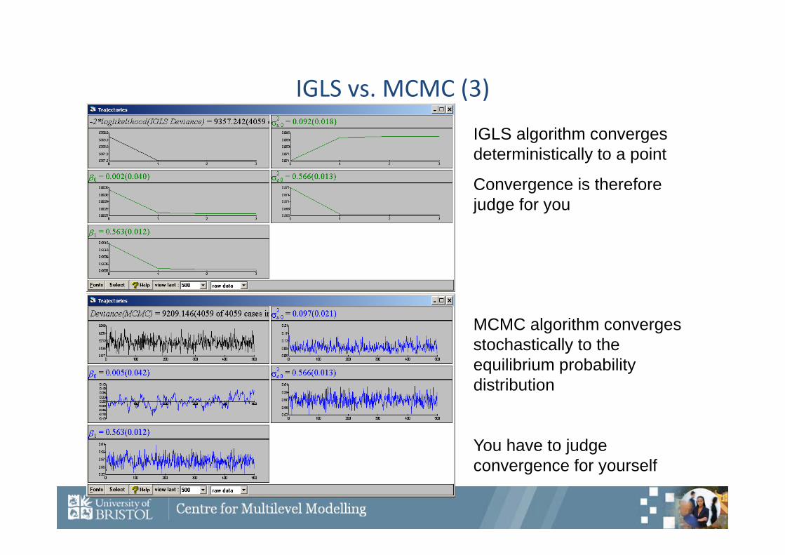
IGLS vs. MCMC (3)
IGLS algorithm converges deterministically to a point
Convergence is therefore judge for you
MCMC algorithm converges stochastically to the equilibrium probability distribution
You have to judge convergence for yourself
Priors
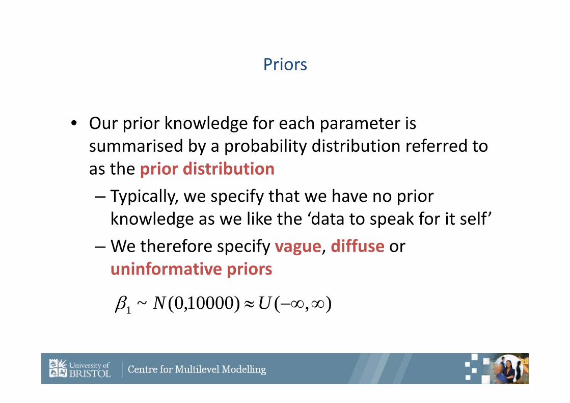
• Our prior knowledge for each parameter is summarised by a probability distribution referred to as the prior distribution– Typically, we specify that we have no prior knowledge as we like the ‘data to speak for it self’
– We therefore specify vague, diffuse or uninformative priors
),()10000,0(~1 UN
MCMC samplers
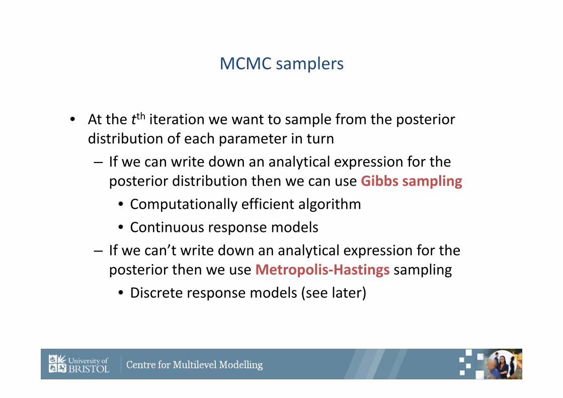
• At the tth iteration we want to sample from the posterior distribution of each parameter in turn– If we can write down an analytical expression for the posterior distribution then we can use Gibbs sampling
• Computationally efficient algorithm• Continuous response models
– If we can’t write down an analytical expression for the posterior then we use Metropolis‐Hastings sampling
• Discrete response models (see later)
Deviance information criterion (DIC) for model comparison
• DIC can be viewed as an AIC or BIC statistic for MCMC
• DIC balances goodness of fit and model complexity(i.e. deviance and number of parameters)
• Want to maximise fit and minimise complexity– Lower deviance and fewer parameters
• So “better” models have smaller DIC• Note that the DIC does not have universal approval!
When to consider usingMCMC Estimation
• Discrete response data (categorical, counts). PQL often gives quick and accurate estimates but a good idea to check against MCMC, especially if you have small clusters – see later
• If you want to obtain accurate confidence intervals for level 2 variances
• Some complex models only estimated using MCMC(e.g. multilevel factor analysis)
• Some models can be fitted more easily using MCMC(e.g. cross‐classified and multiple membership models)