parallel bayesian mcmc imputation for multiple distributed lag

20Parallel Bayesian MCMC Imputation for MultipleDistributed Lag Models: A Case Study inEnvironmental Epidemiology

Brian Caffo, Roger Peng, Francesca Dominici, Thomas A. Louis, and Scott Zeger

20.1 Introduction

Patterned missing covariate data is a challenging issue in environmental epidemiology.For example, particulate matter measures of air pollution are often collected only everythird day or every sixth day, while morbidity and mortality outcomes are collected daily.In this setting, many desirable models cannot be directly fit. We investigate such a setting inso-called “distributed lag” models when the lagged predictor is collected on a cruder timescale than the response. In multi-site studies with complete predictor data at some sites,multilevel models can be used to inform imputation for the sites with missing data.

We focus on the implementation of such multilevel models, in terms of both modeldevelopment and computational implementation of the sampler. Specifically, we paral-lelize single chain runs of sampler. This is of note, since the Markovian structure of Markovchain Monte Carlo (MCMC) samplers typically makes effective parallelization of singlechains difficult. However, the conditional independence relationships of our developedmodel allow us to exploit parallel computing to run the chain. As a first attempt at usingparallel MCMC for Bayesian imputation on such data, this chapter largely represents aproof of principle, though we demonstrate some promising potential for the methodol-ogy. Specifically, the methodology results in proportional decreases in run-time over thenonparallelized version near one over the number of available nodes.

In addition, we describe a novel software implementation of parallelization that isuniquely suited to disk-based shared memory systems. We use a “blackboard” paral-lel computing scheme where shared network storage is a used as a blackboard to tallycurrently completed and queued tasks. This strategy allows for easy addition and sub-traction of compute nodes and control of load balancing. Moreover, it builds in automaticcheckpointing.

Our investigation is motivated by multi-site time series studies of the short-term effectsof air pollution on disease or death rates. A common measure of air pollution used for suchstudies is the amount in micrograms per cubic meter of particulate matter of a specifiedmaximum aerodynamic diameter. We focus on PM2.5 (see Samet et al., 2000). Unfortunately,the definitive source of particulate matter data in the United States, the EnvironmentalProtection Agency’s air pollution network of monitoring stations, collects data only a fewtimes per week at some locations. One of the most frequent observed data patterns for

493

494 Handbook of Markov Chain Monte Carlo

PM2.5 is data being recorded every third day. However, the disease rates that we considerare collected daily.

In this setting, directly fitting a model that includes several lags of PM2.5 simultaneouslyis not possible. Such models are useful, for example, to investigate a cumulative weeklyeffect of air pollution on health. They are also useful to more finely investigate the dynamicsof the relationship between the exposure and response. As an example, one might postulatethat after an increase in air pollution, high air pollution levels on later days may have asmaller impact, as the risk set has been depleted from the initial increase (Dominici et al.,2002; Schwartz, 2000; Zeger et al., 1999).

We focus on distributed lag models that relate the current-day disease rate to particulatematter levels over the past week. That is, our model includes the current day’s PM2.5 levelsas well as the previous six days. While direct estimation of the effect for any particular lagis possible, joint estimation of the distributed lag model is not possible (see Section 20.3).Moreover, missing-data imputation for counties with patterned missing data is difficult.We consider a situation where several independent time series are observed at differentgeographical regions, some with complete PM2.5 data. We use multilevel models to borrowinformation across series to fill in the missing data via Bayesian imputation. The hierarchicalmodel is also used to combine county-specific distributed lag effects into national estimates.

The rest of the chapter is organized as follows. In Section 20.2 we outline the data setused for analysis and follow in Section 20.3 with a discussion of Bayesian imputation.In Section 20.4 we describe the distributed lag models of interest, and in Section 20.5 weillustrate a multiple imputation strategy. Section 20.6 uses the imputation algorithm toanalyze hospitalization rates of chronic obstructive pulmnonary disease (COPD). Finally,Section 20.7 gives some conclusions, discussion and proposals for future work.

20.2 The Data Set

The Johns Hopkins Environmental Biostatistics and Epidemiology Group has assembleda national database comprising time series data on daily hospital admission rates forrespiratory outcomes, fine particles (PM2.5), and weather variables for the 206 largest UScounties having a population larger than 200,000 and with at least one full year of PM2.5data available. The study population, derived from Medicare claims, includes 21 millionadults older than 65 with a place of residence in one of the 206 counties included in thestudy.

Daily counts of hospital admissions and daily number of people enrolled in the cohort areconstructed from the Medicare National Claims History Files. These counts are obtainedfrom billing claims of Medicare enrollees residing in the 206 counties. Each billing claimcontains the following information: date of service, treatment, disease (ICD 9 codes), age,gender, race and place of residence (zip and county).

Air pollution data for fine particles are collected and posted by the United States Environ-mental Protection Agency Aerometric Information Retrieval Service (AIRS, now called theAir Quality System, AQS). To protect against outlying observations, a 10% trimmed mean isused to average across monitors after correction for yearly averages for each monitor. Specif-ically, after removing a smoothly varying annual trend from each monitor time series, thetrimmed mean was computed using the deviations from this smooth trend. Weather data is

Multiple Distributed Lag Models 495

Region

Prop

ortio

n ob

serv

ed

0 50 100 150 200

0.0

0.2

0.4

0.6

0.8

1.0

0

219

438

658

877

1096

NLag 1

FIGURE 20.1Summary of the missing-data pattern. The gray line displays the proportion of the total days in the study withobserved PM2.5 data for each county, with the actual number of days displayed on the right axis. The blackline shows the proportion and count of the days with observed air pollution data where the lag-1 day is alsoobserved.

obtained from the National Weather Monitoring Network which comprises daily temper-ature and daily dew points temperature for approximately 8000 monitoring stations in theUSA. We aggregate data across monitors to obtain temperature time series data for each ofthe 206 counties, of which 196 were used in analysis. Details about aggregation algorithmsfor the air pollution and weather are posted at http://www.biostat.jhsph.edu/MCAPSand further information about data collection is given in Dominici et al. (2006).

Figure 20.1 illustrates the salient features of the missing-data pattern for PM2.5 in thisdatabase. This study considered 1096 monitoring days. Figure 20.1 displays the proportionof the 1096 days with observed PM2.5 data for each county (dark gray line). The associ-ated number of observed days is displayed on the right scale. This figure also displays theproportion of 1096 days with observed PM2.5 data where the lag-1 day was also observed(black line).

The plots show that nearly half of the 196 counties have measurements on roughly onethird of the total possible days. Ninety-six of these counties have over 40% of the air pol-lution data observed and enough instances of seven consecutive observed PM2.5 days toestimate the desired distributed lag model (see Section 20.4). For these counties, any missingdata is often due to a large contiguous block, for example, several weeks where the mon-itor malfunctioned. Such uninformative missing data leaves ample daily measurementsto estimate distributed lag models, so is ignored in our model. The remaining countieshave PM2.5 data collected every third day and possibly also have blocks of missing data,hence have data on less than 33% of the days under study. Because of the systematicallymissing PM2.5 data in these counties, there is little hope of fitting a distributed lag modelwithout borrowing information on the exposure-response curve from daily time seriesdata from other counties. The plot further highlights this by showing that direct estimatesof the lag-1 autocovariances are not available for roughly half of the counties. However,because of the missing-data pattern, all of the counties have direct estimates of the lag-3autocovariances.


20.3 Bayesian Imputation

In this section, we discuss the relative merits of Bayesian imputation. We focus on ourparticular missing-data problem, and refer the reader to Carlin and Louis (2009) andLittle and Rubin (2002) for general introductions to Bayesian statistics, missing data, andcomputation. We argue that imputation for systematic missingness in the predictor timeseries is relevant for distributed lag models, and particularly for the data set in question,while it is less relevant for single-lag models. In this section, we restrict our discussion tothe consideration of a single outcome time series, say Yt, and single predictor time series,Xt. For context, consider the outcome to be the natural log of the county-specific Medi-care emergency admissions rate for COPD, and the predictor to be PM2.5 levels for thatcounty. To make this thought experiment more realistic, let Yt and Xt be the residual timeseries obtained after having regressed out relevant confounding variables. We assume thatthe {Yt} are completely observed and the {Xt} are observed only every third day, so thatX0, X3, X6, . . . are recorded; and we evaluate whether or not to impute the missing predic-tors. In our subsequent analysis of the data, we will treat this problem more formally usingPoisson regression.

20.3.1 Single-Lag Models

A single-lag model relates the Yt to Xt−u for some u = 0, 1, 2, . . . via the mean modelE[Yt] = θuXt−u, when an identity link function is used. We argue that, for any such single-lagmodel, implementing imputation strategies for the missing predictor values is unnecessary.Consider that direct evidence regarding any single-lag model is available in the form of sim-ple lagged cross-correlations. For example, the pairs (Y0, X0), (Y3, X3), (Y6, X6), . . . providedirect evidence for u = 0; the pairs (Y1, X0), (Y4, X3), (Y7, X6), . . . provide direct evidence foru = 1 and so on. Imputing the missing predictors only serves to inject unneeded assump-tions. Furthermore, there is a tradeoff where more variation in the predictor series benefitsthe model’s ability to estimate the associated parameter, yet hampers the ability to imputeinformatively. Hence, in the typical cases where the natural variation in the predictor seriesis large enough to be of interest, we suggest that imputing systematically missing predictordata for single-lag models is not worth the trouble. In less desirable situations with lowvariation in the predictor series, imputation for single-lag models may be of use.

20.3.2 Distributed Lag Models

Now consider a distributed lag model, such as E[Yt] =∑du=0 θuXt−u. Here, if a county

has predictor data recorded every third day, there is no direct information to estimatethis relationship. Specifically, let t = 0, . . ., T − 1 and D be the design matrix associatedwith the distributed lag model and Y be the vector of responses. Then the least squaresestimates of the coefficients are ( 1

T DtD)−1 1T DtY. The off-diagonal terms of 1

T DtD containthe lagged autocovariances in the {Xt} series; 1

T DtY contains the lagged cross-covariancesbetween the {Yt} and {Xt}. As was previously noted, these lagged cross-covariances aredirectly estimable, even with patterned missing data in the predictor series. In contrast, theautocovariances in the predictor series are only directly estimable for lags that are multiplesof 3. Thus, without addressing the missing predictor data, the distributed lag model cannotbe fit. For our data, this would eliminate information from nearly 50% of the countiesstudied. Hence, a study of the utility of predicting the missing data is warranted.


–0.5 0.0 0.5

0.0

0.2

0.4

0.6

0.8

1.0

AR(1) parameter

Like

lihoo

d

FIGURE 20.2Likelihood for theAR(1) coefficient forAR(1) simulated data with an assumed correctly known innovation varianceof 1 and coefficient of 0.5, for three missing-data patterns: completely observed (solid), observed only every threedays (dashed) and observed only every six days (dotted). A solid vertical line denotes the actual coefficient valueof 0.2.

One might consider using a model, such as an AR(p), to extrapolate the missing autocor-relations. However, a single time series with this degree of systematic missingness may nothave enough information to estimate the parameters. Consider an AR(1) process. To illus-trate, Figure 20.2 shows the likelihood for the AR(1) coefficient for data simulated underan AR(1) model with a correctly known innovation variance of 1 and data observed everyday (solid), every third day (dashed) and every sixth day (dotted). Any inference for theAR(1) parameter (at 0.5, depicted with a horizontal line) would be imprecise with the sys-tematically missing data. For the data observed every sixth day, notice that the likelihood ismultimodal and symmetric about zero. This is because the likelihood only depends on theAR coefficient raised to even powers. This poses a problem even for our every-third-daydata, because additional missing observations create patterns of data collected only everysixth day. Such multimodal likelihoods for AR models are described in Wallin and Isaksson(2002) (also see Broersen et al., 2004). In addition, here we assume that the correct model isknown exactly, which is unlikely to be true in practice.

In our data set, there is important information in the counties with completely observeddata that can be used to help choose models for the predictor time series and estimate param-eters. Figure 20.3 demonstrates such model fits with an AR(4) model applied to a detrendedversion of the log of the PM2.5 process. This plot is informative because when the data areavailable only once every third day, it is not possible to estimate the autocorrelation functionusing data only from that county. However, it also illustrates that the population distribu-tion of autoregressive parameters appears to be well defined by the counties with mostlyobserved data. Figure 20.4 shows the estimated residual standard deviations from thesemodel fits, suggesting that these are well estimated even if the autoregressive parametersare not. The data suggest that an AR(1) process is perhaps sufficient, though we continueto focus on AR(4) models to highlight salient points regarding imputation.


0 50 100 150 200

–1.0

–0.5

0.0

0.5

Region

AR

Para

met

er

11

111111111111111111

11111111111111

111

1

1

11111

111

1

111111111111111111

111111

1111111111

11111111111

111

1

1

11

1111

111

1

1

1

1111

1

1

1

1

11

1

111

1

11

11

1

1

11

11

1

1

1

11

1

11

1

1

1

1

1

1

1

1

11

111111

1

11

1

1

11

1

11

1

1

1

1

1

1

1

1

1111

1

1

11

1

11

1

1

11

1

1

1

1

1

22222222222

2

22

222222

222222222

222222

222222222

22222

2

222222222

22222222222222222222222222

22222

222222

2222

2

2

2222

2

2

2

2

2

2

2

22

2

2

2

2

2

2

2

2

2

2

22

2

2

2

2

2

2

22

2

2

2

2

222

2

2

22

2

2

2

222222222

2

2

2

222222222

2

2

2

2

2

222222

2

2

22

2

22

2

2

22

2

2

2

22333

333333333

33333333333333

333333333

33333333

33333333

3333333

33333333333333

333333333333

33333333333

33333

3

3

33333

3

3

3

3

3

33

3

3

3

3

3

3

3

333333

33

3

3

3

33

3

3

3

33333

3

3

3

3

3

33

33333333

33

3

333333

3

33

3333333333333

3

33

3

33

3

3

33

3

3

3

3

3

44444444444444

44444444444444444444

444444444444444

44

4

4444444444444444444

44444444444444444444444444444

4444444

4

44

444

4

4

4

4

4

4

444

4

4

4

4

4

44

4

4

44

4

44444

4

4444

4

4

444

4

4

44

44444

4

4

4

4

4

44

4

4

44

4

44

4

4

4

4444444444

4

444

4

44

4

4

444

FIGURE 20.3Estimated AR(4) coefficients, labeled “1” to “4,” by counties ordered by decreasing percentage of observed datafrom left to right. Roughly the first 100 counties have substantial consecutively observed data to estimate the ARparameters while the remaining 100 do not.

20.4 Model and Notation

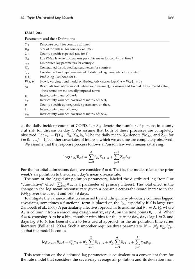
In this section, we present notation and modeling assumptions. A summary of the mostimportant parameters and hyperparameters is given in Table 20.1. Let Yct, for countyc = 0, . . ., C − 1 and day t = 0, . . ., T − 1, denote a response time series of counts, such

0 50 100 150 200

0.1

0.2

0.3

0.4

Region

Varia

nce

FIGURE 20.4Variances from individual autoregressive time series by counties ordered by decreasing percentage of observeddata from left to right.


TABLE 20.1

Parameters and their Definitions

Yct Response count for county c at time t

Rct Size of the risk set for county c at time t

λct County-specific expected rate for Yct

Xct Log PM2.5 level in micrograms per cubic meter for county c at time t

θcu Distributed lag parameters for county c

θ∗cu Constrained distributed lag parameters for county c

θ†cu Constrained and reparameterized distributed lag parameters for county c

�̃(θc) Profile log likelihood for θc

Wct, ψc Slowly varying trend model on the log PM2.5 series log(Xct) = Wctψc + εct

εct Residuals from above model, where we presume ψc is known and fixed at the estimated value;these terms are the actually imputed terms

μ Inter-county mean of the θc

Σθ Inter-county variance–covariance matrix of the θc

αc County-specific autoregressive parameters on the εct

ζ Inter-county mean of the αc

Σα Inter-county variance–covariance matrix of the αc

as the daily incident counts of COPD. Let Rct denote the number of persons in countyc at risk for disease on day t. We assume that both of these processes are completelyobserved. Let λct = E[Yct | Rct, Xct, θc, βc] be the daily mean, Xct denote PM2.5, and Zctj, forj = 0, . . ., J − 1, be other covariates of interest, which we assume are completely observed.

We assume that the response process follows a Poisson law with means satisfying:

log(λct/Rct) =d∑

u=0

θcuXc,t−u +J−1∑j=0

Zctjβcj.

For the hospital admissions data, we consider d = 6. That is, the model relates the priorweek’s air pollution to the current day’s mean disease rate.

The sum of the lagged air pollution parameters, labeled the distributed lag “total” or“cumulative” effect,

∑du=0 θcu, is a parameter of primary interest. The total effect is the

change in the log mean response rate given a one-unit across-the-board increase in thePM2.5 over the current and prior d days.

To mitigate the variance inflation incurred by including many obviously collinear laggedcovariates, sometimes a functional form is placed on the θcu, especially if d is large (seeZanobetti et al., 2000). A particularly effective approach is to assume that θcu = Auθ∗c , whereAu is column u from a smoothing design matrix, say A, on the time points 0, . . ., d. Whend = 6, choosing A to be a bin smoother with bins for the current day, days lag 1 to 2, anddays lag 3 to 6, has been shown to be a useful approach in the air pollution time seriesliterature (Bell et al., 2004). Such a smoother requires three parameters, θ∗c = (θ∗c1, θ∗c2, θ∗c3),so that the model becomes

log(λctr/Rctr) = θ∗c1xct + θ∗c2

2∑u=1

Xc,t−u + θ∗c3

6∑u=3

Xc,t−u +k∑

j=0

zctjβcjr.

This restriction on the distibuted lag parameters is equivalent to a convenient form forthe rate model that considers the seven-day average air pollution and its deviation from


the three-day average and current day:

log(λctr/Rctr) = θ†c1x̄(6)

ct + θ†c2(x̄

(2)ct − x̄(6)

ct )+ θ†c3(xct − x̄(2)

ct )+k∑

j=0

zctjβcjr. (20.1)

Here x̄(k)ct is the average of the current-day and k previous days’ PM2.5 values. These

parameters are related to the θ∗i via the equalities

θ∗c1 =17θ†

c1 +421θ†

c2 +67θ†

c3,

θ∗c2 =17θ†

c1 +421θ†

c2 −17θ†

c3,

θ∗c3 =17θ†

c1 −17θ†

c2 −17θ†

c3.

In this constrained model the total effect is θ†c1 = θ∗c1 + 2θ∗c2 + 4θ∗c3. We use the constrained

and reparameterized specification from Equation 20.1 for analysis. For convenience, wehave dropped the superscript ∗ or † from θ when generically discussing the likelihood orMCMC sampler.

We denote the Poisson log likelihood for county c by �c(θc, βc), where bold face representsa vector of the relevant parameters, such as θc = (θc1, . . ., θcd)

t. Our approach uses Bayesianmethodology to explore the joint likelihood by smoothing parameters across counties. How-ever, the number of nuisance parameters makes implementation and prior specificationunwieldy. Therefore, we replace the county-specific log likelihoods with the associatedprofile log likelihoods:

�̃c(θc) = �c{θc, β̂c(θc)}, where β̂c(θc) = argmaxβc�c(θc, βc).

This step greatly reduces the complexity of the MCMC fitting algorithm. However, it doesso at the cost of theoretical unity, as the profile likelihood used for Bayesian inference isnot a proper likelihood (Monahan and Boos, 1992), as well as computing time. We stipulatethat this choice may impact the validity of the sampler and inference. Currently, we assessvalidity by comparing results with maximum likelihood results for counties with completedata.

The model for the air pollution time series contains trend variables and AR(p) distributederrors. We assume that

log(Xct) = Wctψc + εct, (20.2)

where the εct are a stationary autoregressive process of order p with conditional means andvariances

E[εct|εc,t−1, . . ., εc,t−p] =p∑

j=1

αcjεc,t−j, var(εct|εc,t−1, . . ., εc,t−p) = σ2c .

Here the trend term, Wctψc, represents the slowly varying correlation between air pollutionand seasonality. Specifically, we set Wct to be a natural cubic spline with 24 degrees offreedom per year. Throughout, we set p = 4.


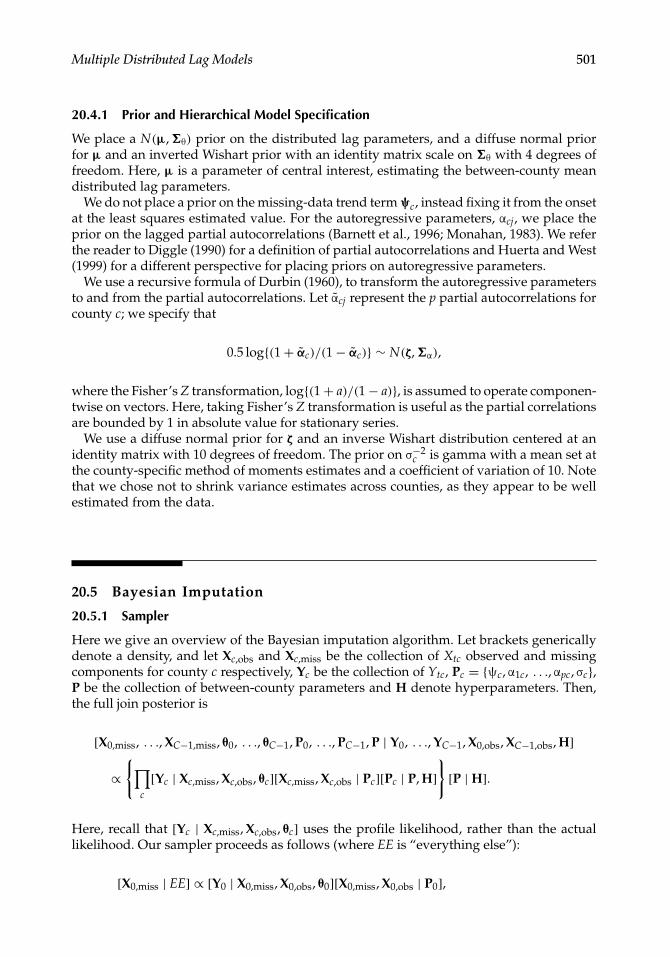
20.4.1 Prior and Hierarchical Model Specification

We place a N(μ, Σθ) prior on the distributed lag parameters, and a diffuse normal priorfor μ and an inverted Wishart prior with an identity matrix scale on Σθ with 4 degrees offreedom. Here, μ is a parameter of central interest, estimating the between-county meandistributed lag parameters.

We do not place a prior on the missing-data trend term ψc, instead fixing it from the onsetat the least squares estimated value. For the autoregressive parameters, αcj, we place theprior on the lagged partial autocorrelations (Barnett et al., 1996; Monahan, 1983). We referthe reader to Diggle (1990) for a definition of partial autocorrelations and Huerta and West(1999) for a different perspective for placing priors on autoregressive parameters.

We use a recursive formula of Durbin (1960), to transform the autoregressive parametersto and from the partial autocorrelations. Let α̃cj represent the p partial autocorrelations forcounty c; we specify that

0.5 log{(1+ α̃c)/(1− α̃c)} ∼ N(ζ, Σα),

where the Fisher’s Z transformation, log{(1+ a)/(1− a)}, is assumed to operate componen-twise on vectors. Here, taking Fisher’s Z transformation is useful as the partial correlationsare bounded by 1 in absolute value for stationary series.

We use a diffuse normal prior for ζ and an inverse Wishart distribution centered at anidentity matrix with 10 degrees of freedom. The prior on σ−2

c is gamma with a mean set atthe county-specific method of moments estimates and a coefficient of variation of 10. Notethat we chose not to shrink variance estimates across counties, as they appear to be wellestimated from the data.

20.5 Bayesian Imputation

20.5.1 Sampler

Here we give an overview of the Bayesian imputation algorithm. Let brackets genericallydenote a density, and let Xc,obs and Xc,miss be the collection of Xtc observed and missingcomponents for county c respectively, Yc be the collection of Ytc, Pc = {ψc, α1c, . . ., αpc, σc},P be the collection of between-county parameters and H denote hyperparameters. Then,the full join posterior is

[X0,miss, . . ., XC−1,miss, θ0, . . ., θC−1, P0, . . ., PC−1, P | Y0, . . ., YC−1, X0,obs, XC−1,obs, H]

∝{∏

c

[Yc | Xc,miss, Xc,obs, θc][Xc,miss, Xc,obs | Pc][Pc | P, H]}[P | H].

Here, recall that [Yc | Xc,miss, Xc,obs, θc] uses the profile likelihood, rather than the actuallikelihood. Our sampler proceeds as follows (where EE is “everything else”):

[X0,miss | EE] ∝ [Y0 | X0,miss, X0,obs, θ0][X0,miss, X0,obs | P0],


[X1,miss | EE] ∝ [Y1 | X0,miss, X0,obs, θ1][X0,miss, X0,obs | P1],...

[XC−1,miss | EE] ∝ [YC | XC−1,miss, XC−1,obs, θC−1][XC−1,miss, XC−1,obs | PC−1],[P0 | EE] ∝ [Y0 | Xc,miss, Xc,obs, θ0][X0,miss, X0,obs | P0],[P1 | EE] ∝ [Y1 | Xc,miss, Xc,obs, θ1][X1,miss, X1,obs | P1],...

[PC−1 | EE] ∝ [YC−1 | XC−1,miss, XC−1,obs, θC][XC−1,miss, XC−1,obs | PC−1],[P | EE] ∝ [Pc | P, H][P | H].

Because of the Gibbs-friendly priors, μ and ζ have multivariate normal full conditionals.Moreover, Σθ and Σα have inverse Wishart full conditionals, while the {σ2

c } have an invertedgamma. The county-specific distributed lag parameters and AR parameters, {θc} and αc,require a Metropolis step. We use a variable-at-a-time, random-walk update. Further detailson the full conditionals are given in the Appendix to this chapter.

The update of the missing data deserves special attention. We use a variable-at-a-timeMetropolis step to impute εtc for each missing day conditional on the remaining. Considerp = 4 and let εc5 be a missing day to be imputed. We use the autoregressive prior for theday under consideration given all of the remaining days as the proposal. For example, thedistribution of εc5 given {εc1, . . ., εc4, ε6, . . ., ε9} is used to generate the proposal for εc5, thatis, the four neighboring days before and after the day under consideration. Because of theAR(4) assumption, this is equivalent to the distribution of ε5 given all of the days. Afterimputation, Xc5 = exp(Wc5ψc + εc5), is calculated. By simulating from the prior distributionof the current missing day given the remainder, only the contribution of Xc5 to the profilelikelihood remains in the Metropolis ratio. To summarize, the distribution of the currentday given the remainder, disregarding the profile likelihood, is used to generate proposals;the profile likelihood is then used in a Metropolis correction. Of course, since PM2.5 has arelatively weak relationship with the response, the acceptance rate is high.

20.5.2 A Parallel Imputation Algorithm

Given the large number of days that need to be imputed for the counties with missing data,and the difficult calculation of the county-specific profile likelihoods, the time for runningsuch a sampler is quite long. In this section we propose a parallel computing approach thatcan greatly speed up computations.

Notice that the conditional-independence structure from Section 20.5.1 illustrates thatall of the county-specific full conditionals are conditionally independent. Thus, the imputationof the missing predictor data, the simulation of the county-specific parameters, and thecalculation of the profile likelihoods can be performed simultaneously. Hence, it representsan ideal instance where we can increase the efficiency of the simulation of a single Markovchain with parallel computation.

To elaborate, let f be the time required to update [P | EE], g0, g1, . . ., gC−1 be the timerequired to transfer the relevant information to and from the separate nodes for parallelprocessing, and h0, h1, . . ., hC−1 be the time required to perform the processing, as depictedin Figure 20.5. Suppose that C nodes are available for computation. Then, conceptually, the


[P | EE] [P | EE]

[X0, miss | EE] [P0 | EE]

[P1 | EE]

[PC–1 | EE]

[X1, miss | EE]

[XC–1, miss | EE]

f f

g0g0

g1

gc–1

......

...

h0

hC–1gC–1

g1h1

and

and

and

FIGURE 20.5Parallel computing diagram.

run-time per parallel MCMC iteration is f + maxc(gc + hc). In contrast, the single processorrun-time would be f +∑c(hc). Clearly, if the transfer times, { gc} are small relative to thecounty-specific processing times, {hc}, then substantial savings can be made by parallelizingthe process, with the gains scaling proportional to the number of conditionally independentfull conditionals. This is exactly the setting of the Medicare claims data, where the profilelikelihood and imputation county-specific calculations are very time-consuming. Of course,this simple schematic is extremely optimistic in not accounting for several factors, such asvariability in the number of available nodes, node-specific run-times and the added timefor the software to manage the parallelization. However, it does suggest that substantialgains can be made with parallelization.

While we know of few implementations of parallel MCMC of this scope, this approachto parallelizing Markov chains and its generalizations has been discussed previously(Kontoghiorghes, 2006; Rosenthal, 2000; Winkler, 2003). Moreover, other approaches couldbe used for parallelizing Markov chains. When applicable, perfect sampling (Fill, 1998; Fillet al., 2000; Propp and Wilson, 1998) could be easily parallelized. Specifically, each perfectsample is an independent and identically distributed draw from the stationary distribu-tion and hence can be generated independently. Also regeneration times (Hobert et al.,2002; Jones et al., 2006; Mykland et al., 1995) create independent tours of the chain fromother regeneration times. Therefore, given a starting value at a regeneration time, the tourscould be generated in parallel. These two techniques have the drawback that a substantialamount of mathematics needs to be addressed to simply implement the sampler prior toany discussion of parallel implementation. A less theoretically justified, yet computation-ally simple, approach parallelizes and combines multiple independent chains (Gelman andRubin, 1992; Geyer, 1992).

Most work on statistical parallel computing algorithms depends on existing network-based parallel computing algorithms, such as Parallel Virtual Machines (Beguelin et al.,1995) or Message Passing Interface (Snir et al., 1995), such as implemented in the Rpackage SNOW (Rossini et al., 2007). These programs are not optimized for particularstatistical problems or computational infrastructures and, furthermore, require directcomputer-to-computer communication. While such parallel computing architectures areused, large computing clusters that employ queuing management software often cannottake advantage of these approaches.

In contrast, our approach uses a disk-based shared memory blackboard system whichrequired building the parallelization software. Specifically in our approach, a collectionof tokens, one for each county, are used to represent which counties currently need pro-cessing. A collection of identical programs, which we refer to as spiders, randomly selecta token from the bin and move it to a bin of tokens representing counties currently being


operated on. We have adopted several strategies to avoid race conditions, where two spi-ders simultaneously attempt to grab the same token, including: using file system locksand creating small random delays before the spider grabs the token. The spider then per-forms the county-specific update and moves its token to another bin of counties withfinished calculations. The spider then goes back to the original bin and repeats the pro-cess. If there are no tokens remaining, the first spider to discover this fact then performsthe national update while the remaining sit idle. It then moves the tokens back to theoriginal bin to restart the process. Disk-based shared memory is used for all of the datatransfer.

The benefits of this strategy for parallel MCMC are many. Notably, nodes or spiderscan be dynamically added or subtracted. Moreover, load balancing can be accomplishedeasily. In addition, the system allowed us to use a storage area network (SAN) as theshared memory resource (blackboard). While having much slower data transfer than directcomputer-to-computer based solutions, this approach allowed us to implement a parallelprogramming in spite of scheduling software that precludes more direct parallelization. Asan added benefit, using the SAN for data transfer builds in automatic checkpointing forthe algorithm. We’ve also found that this approach facilitates good MCMC practice, suchas using the ending value from initial runs as the starting value for final runs. Of course,an overwhelming negative property of this approach is the need to create the custom,setting-specific, parallelization software.

20.6 Analysis of the Medicare Data

We analyzed the Medicare data using our parallel MCMC algorithm. We used 30 processors,resulting in a run-time of 5–10 seconds per MCMC iteration. In contrast, the run-time fora single processor was over 2 minutes. That is, there is a 90% decrease in run-time due toparallelization.

The sampler was run for 13,000 iterations. This number was used as simply the largestfeasible in the time given. Final values from testing-iterations were used as starting values.Trace plots were investigated to evaluate the behavior of the chains, and were also used tochange the step size of the random-walk samplers.

Figure 20.6 displays an example imputation for 1000 monitoring days for a county.The black lines connects observed days while the gray line depicts the estimated trend.The points depict the imputed data set. Figure 20.7 depicts a few days for a county wherepollution data is observed every three days; the separate lines are iterations of the MCMCprocess. These figures illustrate the reasonableness of the imputed data. A possible con-cern is that the imputed data are slightly less variable than the actual data. Moreover, thedata is more regular, without extremely high air pollution days. However, this producesconservatively wider credible intervals for the distributed lag estimates.

Figure 20.8 shows the estimated posterior medians for the exponential of the cumulativeeffect for a 10-unit increase in air pollution, along with 95% credible intervals. The estimatesrange from 0.746 to 1.423. The cumulative effect is interpreted as the relative increase ordecrease in the rate of COPD corresponding to an across-the-board 10-unit increase in PM2.5over the prior six days. Therefore, for example, 1.007 (the national average) represents a 0.7%increase in the rate of COPD per microgram per 10 cubic meter increase in fine particulatematter over six days.


0 200 400 600 800 1000

1020304050

Day

PM2.

5

FIGURE 20.6Example imputation from the MCMC sampler for a specific county. The black line connects observed points whilethe gray line shows the estimated trend. The points are from a specific iteration of the MCMC sampler.

The national estimate,μ1, represents the variance-weighted average of the county-specificcumulative effects. The 95% equi-tail credible interval ranges from an estimated 2.6%decrease to a 4.0% increase in the rate of COPD. The posterior median was a 0.7% increase.In contrast, a meta-analysis model using the maximum likelihood fits and variances foronly those counties with adequate data for fitting the distributed lag model results in aconfidence interval for the national cumulative effect ranging from a 5.1% decrease to a7.5% increase, while the mean is a 1.0% increase. That is, adding the data from the countieswith systematic missing data does not appear to introduce a bias, but does greatly reducethe width of the interval.

The shape of the distributed lag function is of interest to environmental health researchers,as different diseases can have very different profiles, such as rates of hospitalization, recur-rence, and complications. Examining the shape of the distributed lag function can shed lighton the potential relationship of air pollution and the disease. For example, a decline overtime could be evidence of the “harvesting” hypothesis, whereby a large air pollution effectfor early lags would deplete the risk set of its frailest members, through hospitalization ormortality. Hence, the latter days would have lower effects. Figure 20.9 shows the exponentof 10 times the distributed lag parameters’ posterior medians, θ∗c1, θ∗c2, and θ∗c3, by county.Here θ∗c1 is the current-day estimate, while θ∗c2 and θ∗c3 are cumulative effect for days lag1 to 2 and 3 to 6, respectively. The current-day effect tends to be much larger, and morevariable, by county. The comparatively smaller values for the later lags are supportive ofthe harvesting hypothesis, though we emphasize that other mechanisms could be in place.Further, this model is not ideal for studying such phenomena, as the bin smoothing ofthe distributed lag parameters may be too crude to explore the distributed lag function’sshape.

20 30 40 50 600

20

60

100

Day

PM2.

5

FIGURE 20.7Several example imputations for a subset of the days for a county. The lines converge on observed days.


RegionEs

timat

e0.6

1.0

1.4

FIGURE 20.8Estimates and credible intervals for the exponential of the distributed lag cumulative effect by county for a 10-unit increase in air pollution, 10θc1. The solid middle line shows the posterior medians; the gray area shows theestimated 95% equi-tail credible intervals. A horizontal reference line is drawn at 1. Hash marks denote countieswith systematic missing data, where the distributed lag model could not be fit without imputation.

Figure 20.10 shows 95% credible intervals for the AR parameters across counties. Thecounties are organized so that the rightmost 97 counties have the systematic missingdata. Notice that, in these counties, their estimate for the AR(1) parameter is attenuatedtoward zero over the counties with complete data. The estimated posterior median of ζis (0.370,−0.010,−0.011,−0.025)t. The primary AR(1) parameter is slightly below the 0.5,because of the contribution of those counties with missing data. Regardless, we note that

Region

Effe

ct

0.8

1.0

1.2

1.4

Region

Effe

ct

0.8

1.0

1.2

1.4

Region

Effe

ct

0.8

1.0

1.2

1.4

FIGURE 20.9Exponent of ten times the distributed lag parameters’ posterior medians: θ∗c1 (top), θ∗c2 (middle), and θ∗c3 (bottom),by county.


0.25

0.35

0.45

0.55αc2αc1

αc4αc3

–0.10

–0.05

0.00

0.05

–0.05

0.00

0.05

0.10

–0.10

–0.06

–0.02

0.02

FIGURE 20.10Posterior credible intervals for the AR parameters by county.

this shrinkage estimation greatly improves on county-specific estimation (see Figure 20.3)for those cites with incomplete data.

20.7 Summary

In this chapter, we propose an MCMC algorithm for fitting distributed lag models for timeseries with systematically missing predictor data. We emphasize that our analysis onlyscratches the surface for the analysis of the Medicare claims data. One practical issue is theeffect of varying degrees of confounder adjustment, in terms of both the degrees of freedomemployed in nonlinear fits and the confounders included. Moreover, a more thoroughanalysis would consider other health outcomes and different numbers of lags included.Also, commonly air pollution effects are interacted with age or age categories, because ofthe plausibility of different physical responses to air pollution with aging. In addition, thePM measurements are aggregates of several chemical pollutants. Determining the effectsof individual component parts may help explain some of the county variation in the effectof air pollution on health.

The bin smoother on the distributed lag parameters allows for a simpler algorithm andinterpretation. However, more reasonable smoothers, such as setting A to the design matrixfor a regression-spline model, should be considered. This would allow much more accurate


exploration of the shape of the distributed lag model, as well as variations in its shape bycounties.

The use of the profile likelihood instead of the actual likelihood raises numerous issuesand concerns. Foremost is the propriety of the posterior and hence the validity of thesampler and inference. The theoretical consequences of this approach should be evaluated.Moreover, comparisons with other strategies, such as placing independent diffuse priorson the nuisance parameters, are of interest.

Also of interest is to eliminate the attenuation of the estimates of the autoregressiveparameters for the counties with missing data. To highlight this problem more clearly,suppose that instead of 97 counties with missing data, we had 9700 with data recordedevery other day. Then the accurate information regarding ζ and Σα contained in the countieswith complete data would be swamped by the noisy bimodal likelihoods from the countieswith systematic missingness. More elaborate hierarchies on this component of the modelmay allow for the counties with observed data to have control over estimation of theseparameters.

In addition, the potential informativeness of counties having missing data (see Littleand Rubin, 2002) should be investigated. To elaborate, clearly the pattern of missing datais uninformative for any given county; however, whether or not a county collected dataevery day or every third day may be informative. For example, counties with air pollutionslevels well below or above standards may be less likely to collect data every day. Suchmissingness may impact national estimates.

We also did not use external variables to impute the missing predictor data. Ideally, acompletely observed instrumental variable that is causally associated with the predictor,yet not with the response, would be observed. Such variables could be used to imputethe predictor, but would not confound its relationship with the response. However, suchvariables are rarely available. More often variables that are potentially causally associatedwith the predictor are also potentially causally associated with response. For example,seasonality and temperature are thought to be causally associated with PM levels and manyhealth outcomes. Hence, using those variables to impute the missing predictor data wouldimmediately raise the criticism that any association found was due to residual confoundingbetween the response and the variables used for imputation.

These points notwithstanding, this work suggests potential for the ability to impute miss-ing data for distributed lag models. The Bayesian model produces a marked decrease inthe width of the inter-county estimate of the cumulative effect. Moreover, the imputed datasets are consistent with the daily observed data, though perhaps being more regular andless variable. However, we note the bias incurred by lower variability in the imputed airpollution is conservative, and would attenuate the distribute lag effects.

A second accomplishment of this chapter is the parallelization algorithm and softwaredevelopment. The computational overhead for the parallelization software was small, andhence the decrease in run-time was nearly linear with the number of nodes.

Race conditions, times when multiple spiders attempted to access the same token, rep-resent a difficult implementation problem. For example, after the county-specific updatesfinish, all spiders attempt to obtain the token representing the national update simultane-ously. A colleague implementing a similar system proposed a potential solution (FernandoPineda, personal communication). Specifically, he uses atomic operations on a lock fileto only allow access to the bin of tokens to one program at a time. As an analogy, thisapproach has a queue of programs waiting for access to the bins to obtain a token. In con-trast, our approach allows simultaneous access to the bins, thus increasing speed, thoughalso increasing the likelihood of race conditions. A fundamental problem we have yet to


solve is the need for truly atomic operations on networked file systems to prevent theserace conditions. Our use of file system locks when moving files as the proposed atomicoperation made the system very fragile, given the complex nature and inherent lag of anNFS-mounted SAN.

Our current solutions to these problems are inelegant. First, as described earlier, randomwaiting times were added. Secondly, spiders grabbed tokens in a random order. Finally,a worker program was created that searched for and cleaned up lost tokens and ensuredthat the appropriate number of spiders were operational. We are currently experimentingwith the use of an SQL database, with database queries, rather than file manipulations tomanage the tokens.

Appendix: Full Conditionals

We have

θc ∝ exp(

�̃c(θc)− 12(θc − μ)tΣθ(θc − μ)

),

μ ∼ N

{(CΣ−1

θ + G−11

)−1Σ−1θ

C−1∑c=0

θc,(

CΣ−1θ + G−1

1

)−1}

,

Σ−1θ ∼ Wishart

(G2 +

C−1∑c=0

(θc − μ)(θc − μ)t, df1 + C

),

αc ∼ N{(Et

cEc/σ2c +Σ−1

α )−1Etcεc, (Et

cEc/σ2c +Σ−1

α )}

,

ζ ∼ N

{(cΣ−1α + G−1

4

)−1Σ−1α

C−1∑c=0

αc,(

cΣ−1α + G−1

4

)−1Σ−1α

},

Σα ∼ Wishart

(G5 +

C−1∑c=0

(αc − ζ)(αc − ζ)t), df2 + C

),

σ−2c ∼ Γ

⎧⎨⎩C/2+ G6,

C−1∑c=0

(εct −

p∑u=1

εc,t−uαu

)2

+ G7

⎫⎬⎭.

Here εc = (εc1, . . ., εcTc)t, where εct are the residuals after fitting model (Equation 20.2). The

matrix Ec denotes the lagged values of εc. G1, G2, . . . denote generic hyperparameters whosevalues are described in the chapter, while df1 and df2 correspond to prior Wishart degreesof freedom. That is, G1 is the prior variance on μ; G2 represents the Wishart scale matrix forΣθ; (G3, G4) represent the prior means and variance on ζ; G5 represents the Wishart scalematrix for Σα; and G6 and G7 are the gamma shape and rate on σ−2

c .


Acknowledgment

The authors would like to thank Dr. Fernando Pineda for helpful discussions on parallelcomputing.

References

Barnett, G., Kohn, R., and Sheather, S. 1996. Bayesian estimation of an autoregressive model usingMarkov chain Monte Carlo. Journal of Econometrics, 74:237–254.

Beguelin, A., Dongarra, J., Jiang, W., Manchek, R., and Sunderam, V. 1995. PVM: Parallel VirtualMachine: A Users’ Guide and Tutorial for Networked Parallel Computing. MIT Press, Cambridge,MA.

Bell, M., McDermott, A., Zeger, S., Samet, J., and Dominici, F. 2004. Ozone and short-term mortality in95 urban communities, 1987–2000. Journal of the American Medical Association, 292(19):2372–2378.

Broersen, P., de Waele, S., and Bos, R. 2004. Autoregressive spectral analysis when observations aremissing. Automatica, 40(9):1495–1504.

Carlin, B. and Louis, T. 2009. Bayesian Methods for Data Analysis, 3rd edn. Chapman & Hall/CRC Press,Boca Raton, FL.

Diggle, P. 1990. Times Series: A Biostatistical Introduction. Oxford University Press, Oxford.Dominici, F., McDermott, A., Zeger, S., and Samet, J. 2002. On the use of generalized additive models

in time-series studies of air pollution and health. American Journal of Epidemiology, 156(3):193.Dominici, F., Peng, R., Bell, M., Pham, L., McDermott, A., Zeger, S., and Samet, J. 2006. Fine particulate

air pollution and hospital admission for cardiovascular and respiratory diseases. Journal of theAmerican Medical Association, 295(10):1127–1134.

Durbin, J. 1960. The fitting of time series models. International Statistical Review, 28:233–244.Fill, J. 1998. An interruptible algorithm for perfect sampling via Markov chains. Annals of Applied

Probability, 8(1):131–162.Fill, J., Machida, M., Murdoch, D., and Rosenthal, J. 2000. Extension of Fill’s perfect rejection sampling

algorithm to general chains. Random Structures and Algorithms, 17(3–4):290–316.Gelman, A. and Rubin, D. 1992. Inference from iterative simulation using multiple sequences.

Statistical Science, 7:457–511.Geyer, C. 1992. Practical Markov chain Monte Carlo. Statistical Science, 7:473–511.Hobert, J., Jones, G., Presnell, B., and Rosenthal, J. 2002. On the applicability of regenerative simulation

in Markov chain Monte Carlo. Biometrika, 89(4):731–743.Huerta, G. and West, M. 1999. Priors and component structures in autoregressive time series models.

Journal of the Royal Statistical Society, Series B, 61(4):881–899.Jones, G., Haran, M., Caffo, B., and Neath, R. 2006. Fixed-width output analysis for Markov chain

Monte Carlo. Journal of the American Statistical Association, 101(476):1537–1547.Kontoghiorghes, E. 2006. Handbook of Parallel Computing and Statistics. Chapman & Hall/CRC, Boca

Raton, FL.Little, R. and Rubin, D. 2002. Statistical Analysis with Missing Data, 2nd edn. Wiley, Hoboken, NJ.Monahan, J. 1983. Fully Bayesian analysis of ARMAtime series models. Journal of Econometrics, 21:307–

331.Monahan, J. and Boos, D. 1992. Proper likelihoods for Bayesian analysis. Biometrika, 79(2):271–278.Mykland, P., Tierney, L., and Yu, B. 1995. Regeneration in Markov chain samplers. Journal of the

American Statistical Association, 90(429):233–241.Propp, J. and Wilson, D. 1998. How to get a perfectly random sample from a generic Markov chain

and generate a random spanning tree of a directed graph. Journal of Algorithms, 27(2):170–217.


Rosenthal, J. 2000. Parallel computing and Monte Carlo algorithms. Far East Journal of TheoreticalStatistics, 4(2):207–236.

Rossini, A., Tierney, L., and Li, N. 2007. Simple parallel statistical computing in R. Journal ofComputational and Graphical Statistics, 16(2):399.

Samet, J., Dominici, F., Currieo, F., Coursac, I., and Zeger, S. 2000. Fine particulate air pollution andmortality in 20 U.S. cities 1987-1994. New England Journal of Medicine, 343(24):1742–1749.

Schwartz, J. 2000. Harvesting and long term exposure effects in the relation between air pollution andmortality. American Journal of Epidemiology, 151(5):440.

Snir, M., Otto, S., Walker, D., Dongarra, J., and Huss-Lederman, S. 1995. MPI: The Complete Reference.MIT Press, Cambridge, MA.

Wallin, R. and Isaksson, A. 2002. Multiple optima in identification of ARX models subject to missingdata. EURASIP Journal on Applied Signal Processing, 1:30–37.

Winkler, G. 2003. Image Analysis, Random Fields, and Dynamic Monte Carlo Methods, 2nd edn. Springer,Berlin.

Zanobetti, A., Wand, M. P., Schwartz, J., and Ryan, L. M. 2000. Generalized additive distributed lagmodels: Quantifying mortality displacement. Biostatistics, 1(3):279–292.

Zeger, S., Dominici, F., and Samet, J. 1999. Harvesting-resistant estimates of air pollution effects onmortality. Epidemiology, 10(2):171.

parallel bayesian mcmc imputation for multiple distributed lag

Documents