An introduction to adaptive MCMC

Gareth Roberts

MIRAW Day on Monte Carlo methodsMarch 2011

Mainly joint work with Jeff Rosenthal.

http://www2.warwick.ac.uk/fac/sci/statistics/crism/

Conferences and workshops

Academic visitor programme.

Workshops coming up:

March 28 - April 1, INfER, Statistics for infectious diseasesApril 5 - 7, WOGAS III, geometry and statisticsApril 13, Prior elicitation

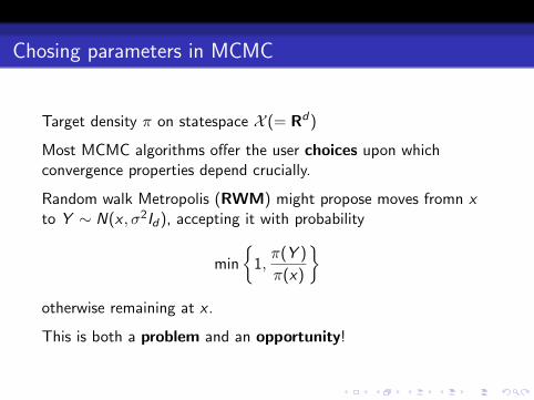
Chosing parameters in MCMC

Target density π on statespace X (= Rd)

Most MCMC algorithms offer the user choices upon whichconvergence properties depend crucially.

Random walk Metropolis (RWM) might propose moves fromn xto Y ∼ N(x , σ2Id), accepting it with probability

min

{1,π(Y )

π(x)

}otherwise remaining at x .

This is both a problem and an opportunity!

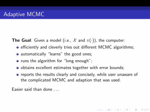
Adaptive MCMC

The Goal: Given a model (i.e., X and π(·)), the computer:

efficiently and cleverly tries out different MCMC algorithms;

automatically “learns” the good ones;

runs the algorithm for “long enough”;

obtains excellent estimates together with error bounds;

reports the results clearly and concisely, while user unaware ofthe complicated MCMC and adaption that was used.

Easier said than done . . .

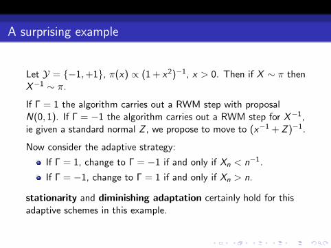
A surprising example

Let Y = {−1,+1}, π(x) ∝ (1 + x2)−1, x > 0. Then if X ∼ π thenX−1 ∼ π.

If Γ = 1 the algorithm carries out a RWM step with proposalN(0, 1). If Γ = −1 the algorithm carries out a RWM step for X−1,ie given a standard normal Z , we propose to move to (x−1 + Z )−1.

Now consider the adaptive strategy:

If Γ = 1, change to Γ = −1 if and only if Xn < n−1.

If Γ = −1, change to Γ = 1 if and only if Xn > n.

stationarity and diminishing adaptation certainly hold for thisadaptive schemes in this example.

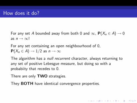
How does it do?

For any set A bounded away from both 0 and ∞, P(Xn ∈ A)→ 0as n→∞!

For any set containing an open neighbourhood of 0,P(Xn ∈ A)→ 1/2 as n→∞

The algorithm has a null recurrent character, always returning toany set of positive Lebesgue measure, but doing so with aprobabiity that recedes to 0.

There are only TWO strategies.

They BOTH have identical convergence properties.

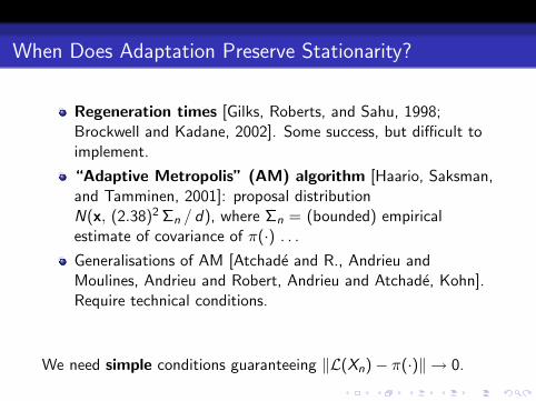
When Does Adaptation Preserve Stationarity?

Regeneration times [Gilks, Roberts, and Sahu, 1998;Brockwell and Kadane, 2002]. Some success, but difficult toimplement.

“Adaptive Metropolis” (AM) algorithm [Haario, Saksman,and Tamminen, 2001]: proposal distributionN(x, (2.38)2 Σn / d), where Σn = (bounded) empiricalestimate of covariance of π(·) . . .

Generalisations of AM [Atchade and R., Andrieu andMoulines, Andrieu and Robert, Andrieu and Atchade, Kohn].Require technical conditions.

We need simple conditions guaranteeing ‖L(Xn)− π(·)‖ → 0.

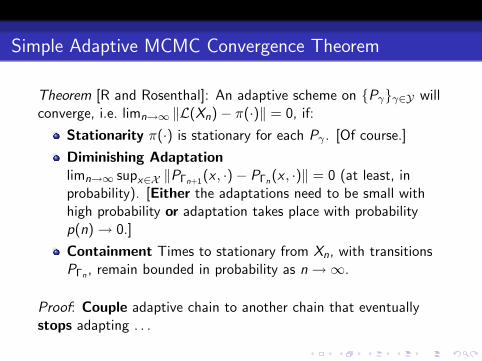
Simple Adaptive MCMC Convergence Theorem

Theorem [R and Rosenthal]: An adaptive scheme on {Pγ}γ∈Y willconverge, i.e. limn→∞ ‖L(Xn)− π(·)‖ = 0, if:

Stationarity π(·) is stationary for each Pγ . [Of course.]

Diminishing Adaptationlimn→∞ supx∈X ‖PΓn+1(x , ·)− PΓn(x , ·)‖ = 0 (at least, inprobability). [Either the adaptations need to be small withhigh probability or adaptation takes place with probabilityp(n)→ 0.]

Containment Times to stationary from Xn, with transitionsPΓn , remain bounded in probability as n→∞.

Proof: Couple adaptive chain to another chain that eventuallystops adapting . . .

Ergodicity

Under stationarity, adaptation and containment also get

limt→∞∑t

n=1 f (Xn)

t= π(f ) in probability

for any bounded function f .

However convergence for all L1 functions does not follow(counterexample by Chao, Toronto).

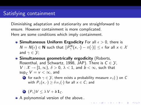
Satisfying containment

Diminishing adaptation and stationarity are straighforward toensure. However containment is more complicated.Here are some conditions which imply containment.

Simultaneous Uniform Ergodicity For all ε > 0, there isN = N(ε) ∈ N such that ‖PN

γ (x , ·)− π(·)‖ ≤ ε for all x ∈ Xand γ ∈ Y;

Simultaneous geometrically ergodicity (Roberts,Rosenthal, and Schwartz, 1998, JAP). There is C ∈ Y,V : X → [1,∞), δ > 0, λ < 1, and b <∞, such thatsupC V = v <∞, and

1 for each γ ∈ Y, there exists a probability measure νγ(·) on Cwith Pγ(x , ·) ≥ δ νγ(·) for all x ∈ C ; and

2 (Pγ)V ≤ λV + b 1C .

A polynomnial version of the above..

Common drift function conditions

Simultaneous geometric ergodicity and simultaneous polynomialergodicity are examples of common drift function conditions.

Such conditions say that all Markov kernels can be considered tobe pushing towards the same small set as measured by thecommon drift condition.

When different chains have different ways of moving towards π,disaster can occur!

A surprising example (cont)

Let Y = {−1,+1}, π(x) ∝ (1 + x2)−1, x > 0. Then if X ∼ π thenX−1 ∼ π.

If Γ = 1 the algorithm carries out a RWM step with proposalN(0, 1). If Γ = −1 the algorithm carries out a RWM step for X−1,ie given a standard normal Z , we propose to move to (x−1 + Z )−1.

Now consider the adaptive strategy:

If Γ = 1, change to Γ = −1 if and only if Xn < n−1.

If Γ = −1, change to Γ = 1 if and only if Xn > n.

Thus stationarity and diminishing adaptation certainly hold forthis adaptive schemes.

What goes wrong?

Containment must fail. But how?

For Γ = 1, any set bounded away from ∞ is small. [P(x , ·) ≥ εν(·)for all x ∈ the small set.]

For Γ = −1, any set bounded away from 0 is small.

A natural drift function for Γ = 1 diverges at x →∞, and isbounded on bounded regions. A natural drift function for Γ = −1is unbounded as x → 0, and is bounded on regions bounded awayfrom zero.

Cannot do both with a single drift function!

Common drift functions for RWM

If {Pγ} are a class of full-dimensional RWMs, a natural driftfunction is often π(x)−1/2. For instance if the contours of π aresufficiently regular in the tails, and Pγ represents RWM withproposal variance matrix γ such that there exists a constant ε with

εId ≤ γ ≤ ε−1Id

(with the inequalities understood in a positive-definite sense).This is useful for the adaptive Metropolis (AM) example later.[This is based on recent work by R + Rosenthal extendingR+Tweedie, 1996, Biometrika.]

Common drift functions for single component Metropolisupdates

Consider single component Metropolis updates.Easiest to prove for random scan Metropolis which just chooses acomponent to update at random, and then updates according to a1-dimensional Metropolis.

Again we can use V (x) = π(x)−1/2.

[This is based on recent work by Latuszynski, R + Rosenthalextending R+Rosenthal, 1998, AnnAP.]

Scaling proposals

π is a d-dimensional probability density function with respect tod-dimensional Lebesgue measure. Consider

RWM Propose new value Y ∼ N(x, γ) [γ is a matrix here.]

MwG Choose a component at random, i say, and updateXi |X−i according to a one-dimensional Metropolis updatewith proposal N(xi , γi ). [γ is a vector here!]

Lang Langevin update: propose new value fromN(x + γ∇ log π(x)/2, γ). [γ is a matrix here!]

What scaling theory tells us, RWM case ...

R, Rosenthal, Sherlock, Pete Neal, Bedard, Gelman, Gilks...For RWM, we set γ = δ2 × V for a scalar δ.

For continuous densities, and for fixed V , the scalaroptimisation is often achieved by finding the algorithm whichachieves an acceptance rate somewhere between 0.15 and 0.4.In many limiting cases (as d →∞) the optimal value is 0.234.

”0.234” breaks down only when V is an extremely poorapproximation to the target distribution covariance Σ.

For Gaussian targets, when V = Σ, the optimal value of δ is

δ = 2.38/d1/2 .

In the Gaussian case we can exactly quantify the cost ofhaving V different to Σ:

R =(∑λ2

i /d)1/2∑λi/d

=L2

L1

where {λi} denote the eigenvalues of V 1/2Σ−1/2.

For densities with discontinuities, the problem is far morecomplex. For certain problems, the optimal limitingacceptance probability is 0.13.

Optimal scaling is robust to transience.

What scaling theory tells us, MwG case ...

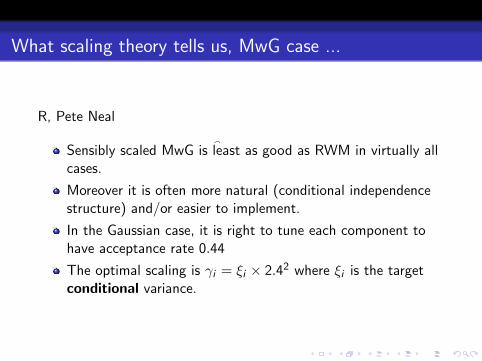
R, Pete Neal

Sensibly scaled MwG is �least as good as RWM in virtually allcases.

Moreover it is often more natural (conditional independencestructure) and/or easier to implement.

In the Gaussian case, it is right to tune each component tohave acceptance rate 0.44

The optimal scaling is γi = ξi × 2.42 where ξi is the targetconditional variance.

What scaling theory tells us, Lang case ...

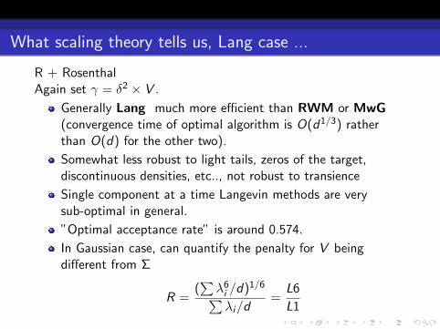
R + RosenthalAgain set γ = δ2 × V .

Generally Lang much more efficient than RWM or MwG(convergence time of optimal algorithm is O(d1/3) ratherthan O(d) for the other two).

Somewhat less robust to light tails, zeros of the target,discontinuous densities, etc.., not robust to transience

Single component at a time Langevin methods are verysub-optimal in general.

”Optimal acceptance rate” is around 0.574.

In Gaussian case, can quantify the penalty for V beingdifferent from Σ

R =(∑λ6

i /d)1/6∑λi/d

=L6

L1

Adaptive Metropolis (AM) Example

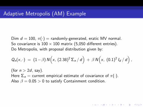
Dim d = 100, π(·) = randomly-generated, eratic MV normal.So covariance is 100× 100 matrix (5,050 different entries).Do Metropolis, with proposal distribution given by:

Qn(x , ·) = (1−β) N(

x , (2.38)2 Σn / d)

+ β N(

x , (0.1)2 Id / d),

(for n > 2d , say).Here Σn = current empirical estimate of covariance of π(·).Also β = 0.05 > 0 to satisfy Containment condition.

Adaptive Metropolis Example (cont’d)

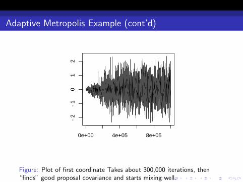
0e+00 4e+05 8e+05

−2

−1

01

2

Figure: Plot of first coordinate Takes about 300,000 iterations, then“finds” good proposal covariance and starts mixing well.

Adaptive Metropolis Example (cont’d)

0e+00 4e+05 8e+05

050

100

150

200

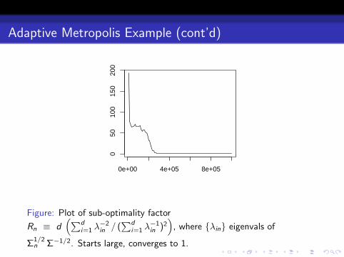
Figure: Plot of sub-optimality factor

Rn ≡ d(∑d

i=1 λ−2in / (

∑di=1 λ

−1in )2

), where {λin} eigenvals of

Σ1/2n Σ−1/2. Starts large, converges to 1.

Adaptive Metropolis-within-Gibbs Strategies

Possible strategies for each component separately:

1 adapt proposal variance in particular component to match theempirical variance (SCAM);

2 adapt component acceptance probability to be around 0.44(AMwG);

3 try to estimate some kind of average conditional varianceempirically and fit to proposal variance.

Our empirical evidence suggests that AMwG uusally beats SCAM,but all strategies can be tested by problems for whichheterogenous variances are required.

In the Gaussian case, can show that (2) and (3) converge to“optimal” MwG.

Adaptive Metropolis-within-Gibbs Example

Propose move for each coordinate separately.Propose increment N(0, e2 lsi ) for i th coord.

Start with lsi ≡ 0 (say).Adapt each lsi , in batches, to seek 0.44 acceptance ratio(approximately optimal for one-dim proposals).

Test on Variance Components Model, with K = 500 locationparameters (so dim = 503), and data Yij ∼ N(µi , 102) for1 ≤ i ≤ K and 1 ≤ j ≤ Ji , where the Ji are chosen between 5 and500.

Metropolis-within-Gibbs (cont’d)

0 50000 150000 250000

0.0

0.5

1.0

1.5

2.0

2.5

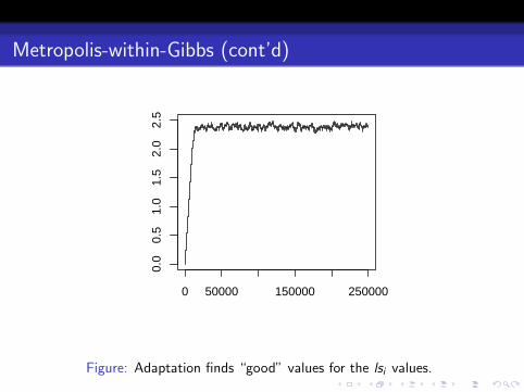
Figure: Adaptation finds “good” values for the lsi values.

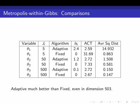
Metropolis-within-Gibbs: Comparisons

Variable Ji Algorithm lsi ACT Avr Sq Dist

θ1 5 Adaptive 2.4 2.59 14.932θ1 5 Fixed 0 31.69 0.863θ2 50 Adaptive 1.2 2.72 1.508θ2 50 Fixed 0 7.33 0.581θ3 500 Adaptive 0.1 2.72 0.150θ3 500 Fixed 0 2.67 0.147

Adaptive much better than Fixed, even in dimension 503.

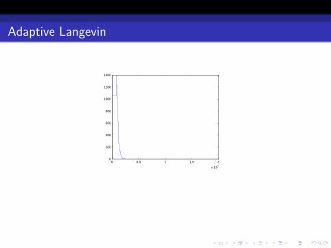
Adaptive Langevin

0 0.5 1 1.5 2

x 104

0

200

400

600

800

1000

1200

1400

Figure: Adaptive Langevin R value, d = 20

0 0.5 1 1.5 2

x 104

−40

−30

−20

−10

0

10

20

30

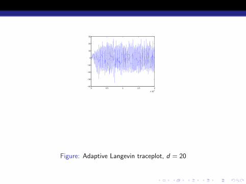
Figure: Adaptive Langevin traceplot, d = 20

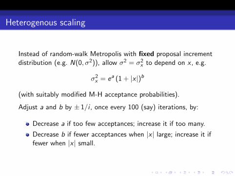
Heterogenous scaling

Instead of random-walk Metropolis with fixed proposal incrementdistribution (e.g. N(0, σ2)), allow σ2 = σ2

x to depend on x , e.g.

σ2x = ea (1 + |x |)b

(with suitably modified M-H acceptance probabilities).

Adjust a and b by ± 1/i , once every 100 (say) iterations, by:

Decrease a if too few acceptances; increase it if too many.

Decrease b if fewer acceptances when |x | large; increase it iffewer when |x | small.

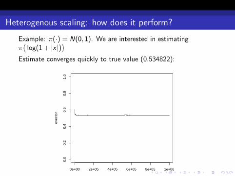
Heterogenous scaling: how does it perform?

Example: π(·) = N(0, 1). We are interested in estimatingπ(

log(1 + |x |))

Estimate converges quickly to true value (0.534822):

0e+00 2e+05 4e+05 6e+05 8e+05 1e+06

0.0

0.2

0.4

0.6

0.8

1.0

xvals

evec

tor

Figure:

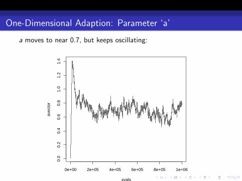
One-Dimensional Adaption: Parameter ‘a’

a moves to near 0.7, but keeps oscillating:

0e+00 2e+05 4e+05 6e+05 8e+05 1e+06

0.0

0.2

0.4

0.6

0.8

1.0

1.2

1.4

xvals

avec

tor

Figure:

One-Dimensional Adaption: Parameter ‘b’

b moves to near 1.5, but keeps oscillating:

0e+00 2e+05 4e+05 6e+05 8e+05 1e+06

0.0

0.5

1.0

1.5

xvals

bvec

tor

Figure:

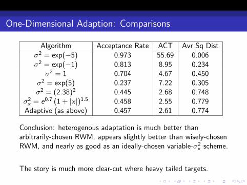
One-Dimensional Adaption: Comparisons

Algorithm Acceptance Rate ACT Avr Sq Dist

σ2 = exp(−5) 0.973 55.69 0.006σ2 = exp(−1) 0.813 8.95 0.234

σ2 = 1 0.704 4.67 0.450σ2 = exp(5) 0.237 7.22 0.305σ2 = (2.38)2 0.445 2.68 0.748

σ2x = e0.7 (1 + |x |)1.5 0.458 2.55 0.779

Adaptive (as above) 0.457 2.61 0.774

Conclusion: heterogenous adaptation is much better thanarbitrarily-chosen RWM, appears slightly better than wisely-chosenRWM, and nearly as good as an ideally-chosen variable-σ2

x scheme.

The story is much more clear-cut where heavy tailed targets.

Some conclusions

Good progress has been made towards finding simple usableconditions for adaptation, at least for standard algorithms.Further progress is subject of joint work with Krys Latuszynskiand Jeff Rosenthal.

Algorithm families with different small sets and driftconditions are dangerous!

In practice, Adaptive MCMC is very easy. Currentimplentation in some forms of BUGS.

More complex adaptive schemes often require individualconvergence results (eg for adaptive Gibbs samplers and itsvariants in work with Krys and Jeff, and work by Atchade andLiu on the Wang Landau algorithm.