Physica D 269 (2014) 42–47

Contents lists available at ScienceDirect

Physica D

journal homepage: www.elsevier.com/locate/physd

Exact significance test for Markov orderS.D. Pethel a,∗, D.W. Hahs b

a U.S. Army RDECOM, RDMR-WDS-W, Redstone Arsenal, AL 35898, USAb Torch Technologies, Inc., Huntsville, AL 35802, USA

h i g h l i g h t s

• We give a hypothesis test of Markov order from time series data.• A novel and efficient algorithm for generating surrogate data is introduced.• Surrogate data enables exact computation of null hypothesis p-values even for small data sets.

a r t i c l e i n f o

Article history:Received 1 March 2013Received in revised form17 September 2013Accepted 22 November 2013Available online 1 December 2013Communicated by A.C. Newell

Keywords:Markov orderHypothesis testWhittle’s formula

a b s t r a c t

We describe an exact significance test of the null hypothesis that a Markov chain is nth order. Theprocedure utilizes surrogate data to yield an exact test statistic distribution valid for any sample size.Surrogate data are generated using a novel algorithm that guarantees, per shot, a uniform sampling fromthe set of sequences that exactly match the nth order properties of the observed data. Using the test, theMarkov order of Tel Aviv rainfall data is examined.

Published by Elsevier B.V.

1. Introduction

It often happens that it is useful to describe a process as a setof discrete states with probabilistic transitions. Examples aboundin various fields such as the study of chemical processes [1], DNAsequences [2], finance [3], and nonlinear dynamics [4], amongothers. If the transition probability to the next state is conditionedonly on the present state we call this model a Markov chain.An nth-order Markov chain is a generalization that includes thepast n states in the transition probability. When the conditionalprobabilities are not otherwise given, they are estimated from atime series of observations.

If the order of theMarkov chain is in question, there are varioustests and criteria available to narrow down the options. The classi-cal approach is to formulate the question as a hypothesis test thata chain is nth order and specify a discriminating test statistic [5].Often the chosen test statistic has a known limiting distribution,such as χ2, fromwhich a p-value is calculated [6]. The use of a lim-iting distribution is inexact because it is only attained for infinite

∗ Corresponding author. Tel.: +1 2568429734.E-mail addresses: shawn.pethel@us.army.mil, shawn.d.pethel.civ@mail.mil

(S.D. Pethel), daniel.hahs@us.army.mil (D.W. Hahs).

0167-2789/$ – see front matter. Published by Elsevier B.V.http://dx.doi.org/10.1016/j.physd.2013.11.014

data sets. For small data sets it may be a very poor approximation.In this article we develop a procedure to compute p-values that areexact, even for small data sets.

The p-value is the probability, assuming the null hypothesis, ofthe test statistic attaining its observed value or one more extreme.It is not the probability of the null hypothesis being correct. Whilea very small p-value leads one to reject the null hypothesis, alarge p-value only implies that the data is consistent with the nullhypothesis, not that the null hypothesis should be accepted. Inaddition, the significance threshold for rejection is entirely up tothe user to decide.

There are alternative approaches that provide a positive answerto order selection. The Akaike information criterion (AIC), theBayesian information criterion (BIC), and others [7–10] producerankings over multiple orders based on their relative likelihoodsand have built-in penalties for over-fitting. Unfortunately, theseapproaches rely on approximations that are only valid in the limitof large samples. In small sample situations one cannot be sure oftheir efficacy.

In spite of the shortcomings of hypothesis tests, there is anadvantage in that it is possible, in principle, to perform an exactMarkov order significance test that is valid for any sample size. In-stead of relying on asymptotic properties, the test statistic distribu-tion is discovered by sampling from the set of sequences (referred

S.D. Pethel, D.W. Hahs / Physica D 269 (2014) 42–47 43

to here as surrogates) that exactlymatch the nth order properties ofthe observed time series [11]. The challenge is in efficiently gener-ating a large number of such samples, especially for higher orders.To our knowledge no solution to this problem has been reported inthe literature.

The contribution of this work is a surrogate data procedure thathas ideal properties: each sample surrogate has exactly the sametransition counts as the observed sequence, one sample is gener-ated per shot, samples are uniformly selected from the set of allpossible surrogate sequences, computation time increases linearlywith the length of the sequence, and any order can be accommo-dated. Armedwith this new procedure it is now straightforward tocompute the p-value of a Markov order null hypothesis exactly forany size data set. The obtained value may be used for significancetesting in the standard way (as we do here) or as part of a moregeneral procedure for model selection.

We first describe how to do hypothesis testing of Markov orderusing the χ2 statistic, for which the distribution is known in thelarge sample limit. Next we describe the method of surrogatedata generation based on Whittle’s formula. Then we comparethe χ2 statistic in large and small sample cases using both theasymptotic distribution and the exact distribution obtained fromthe surrogates. Finally, we analyze Tel Aviv rainfall data in whichAIC and BIC give differing results and discuss the use of p-values inthis situation.

2. Testing Markov order using the χ2 statistic

A sequence of observations x = {x1 . . . xN} form aMarkov chainof order n if the conditional probability satisfies

p(xt+1|xt , xt−1 . . .) = p(xt+1|xt . . . xt−n+1), (1)

for all n < t ≤ N . For convenience we will label the states eachmeasurement can take by positive integers up to S. A sequence ofdiscrete measurements may come from a process that is naturallydiscrete, such as a DNA sequence, or from a continuous processthat has been discretized by an analog-to-digitalmeasuring device.Unless otherwise specified a Markov process is assumed to be firstorder (n = 1). This means that the transition probabilities to afuture state depend only on the present state and not on priorstates. An nth order process can always be cast as first order bygrouping the present statewith the relevant past states into aword,in which case the number of states can be up to Sn. A processthat has no dependence on past or present (such as a random iidprocess) is said to be zeroth order.

To perform an nth order null hypothesis test it is necessary tocompute the distribution of a suitable higher order statistic. If theobserved higher order statistic is sufficiently unlikely, then the nullhypothesis is rejected. The probability, given the null hypothesis, ofthe test statistic attaining the observed value or onemore extremeis referred to as the p-value. Typically, a p-value less than or equalto 0.05 is taken as grounds to reject the null hypothesis.

Let us begin with the assumption that {xt} is an observedsequence from a first order Markov process (n = 1) and calculatethe p-value of a second order statistic using a χ2 distribution. Thenull hypothesis is

p(xt+1 = i|xt = j, xt−1 = k) = p(xt+1 = i|xt = j), (2)

or using Bayes’ rule

p(xt+1 = i, xt = j, xt−1 = k)

=p(xt+1 = i, xt = j)p(xt = j, xt−1 = k)

p(xt = j). (3)

The l.h.s. of (3) multiplied by N − 2 is the expected number oftimes the word (xt+1 = i, xt = j, xt−1 = k) appears in thedata given the null hypothesis. The quantities on the r.h.s. are notexpected values; they are taken from the observed sequence. LetEw be the expectedword countwhere

Ew = N−2 andw indexes

the set of all words for which the expected count is greater thanzero. Similarly, let Ow ≥ 0 be the corresponding count from theobserved data. We can now define the observed χ2 test statistic

χ2obs =

w

(Ew − Ow)2

Ew

, (4)

which is ameasure of the deviation of the observed count from theexpected. The first order assumption does not uniquely determinethe second order statistics; there is some freedom for χ2 tovary from shot to shot even assuming the null hypothesis. Theadvantage of the χ2 statistic is that, given the degrees of freedomd, the distribution f (χ2

; d) is known in the limit N → ∞. Thep-value is then obtained by integrating f (χ2) over χ2

≥ χ2obs.

An issue requiring some discussion is how to compute thedegrees of freedom d needed to determine the χ2 distribution. Totest the nth-order hypothesis we count the observed k = n + 1length words and compute the expected k + 1 length words.Assuming all Sk length k words are present in the data, let F be aSk×Sk transition countmatrix. The (i, j)th entry of F is the numberof times word i transitions to word j. Because consecutive wordsoverlap and differ by only one symbol, there are at most S nonzeroentries in each row and column of F . It is helpful to rearrange Finto block diagonal formwith k S×S blocks. In each block both therows and columnsmust add up to the corresponding length kwordcount. Taking into account rowand columndependencies leaves uswith Sk−1(S − 1)2 degrees of freedom for k > 0, and (S − 1)2 fork = 0 [12]. In the case that not all length k words are present inthe observed data, F will be smaller than Sk × Sk and the blocksalong the diagonal may be of differing size. If the size of the bthblock is rb × cb, then the total number of degrees of freedom d is

(rb − 1)(cb − 1).

3. Exact test using surrogate data

The hypothesis test as described above is not exact; it relies onthe χ2 distribution valid in the asymptotic limit of infinite data.To discover the exact distribution for finite data it is necessaryto evaluate χ2 for all possible sequences that satisfy the nullhypothesis. For the first order hypothesis these sequences haveexactly the same joint probabilities shown on the r.h.s. of (3). LetFij be the number of times word i transitions to word j in x, and letΓ (x) represent the set of sequences with the same F and the samebeginning and end states as the observed sequence x.

The number of sequences that have the word transition countF and begin with state u and end with state v is given by Whittle’sformula [13]:

Nuv(F) =ΠiFi·!ΠijFij!

Cvu (5)

where Fi· is the sum of row i and Cvu is the (v, u)th cofactor of thematrix

F∗

ij =

δij − Fij/Fi· if Fi· > 0,δij if Fi· = 0. (6)

As an example, consider the following sequence of twelve bi-nary observations:

x = {0 1 1 0 1 0 1 1 1 0 0 1}. (7)

44 S.D. Pethel, D.W. Hahs / Physica D 269 (2014) 42–47

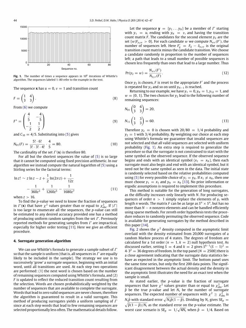
Fig. 1. The number of times a sequence appears in 106 iterations of Whittle’salgorithm. The sequences labeled 1–80 refer to the example in the text.

The sequence x has u = 0, v = 1 and transition count

F =

1 43 3

. (8)

From (6) we compute

F∗=

45

−45

−12

12

(9)

and C10 = 4/5. Substituting into (5) gives

N01(F) =5! · 6!

3! · 3! · 4!·45

= 80. (10)

The cardinality of the set Γ (x) is therefore 80.For all but the shortest sequences the value of (5) is so large

that it cannot be computed using fixed precision arithmetic. In ouralgorithmwe instead compute the natural logarithm of (5) using aStirling series for the factorial terms:

ln z! ∼ z ln z − z +12ln(2πz) +

112z

−1

360z3+

11260z5

−1

1680z7(11)

when z > 16.To find the p-value we need to know the fraction of sequences

in Γ (x) that have χ2 values greater than or equal to χ2obs. If |Γ |

is too large to enumerate all the sequences, the p-value can stillbe estimated to any desired accuracy provided one has a methodof producing uniform random samples from the set Γ . Previouslyreported methods for generating samples from Γ are impractical,especially for higher order testing [11]. Here we give an efficientprocedure.

4. Surrogate generation algorithm

We can use Whittle’s formula to generate a sample subset of Γso that the sample is uniform (that is, all sequences inΓ are equallylikely to be included in the sample). The strategy we use is tosuccessively ‘grow’ a surrogate sequence, beginning with an initialword, until all transitions are used. At each step two operationsare performed: (1) the next word is chosen based on the numberof remaining sequences computed usingWhittle’s formula, and (2)F is updated to reflect the reduced transition count resulting fromthe selection. Words are chosen probabilistically weighted by thenumber of sequences that are available to complete the surrogate.Words that lead to zero valid sequences are never chosen, thereforethe algorithm is guaranteed to result in a valid surrogate. Thismethod of producing surrogates yields a uniform sampling of Γ

since at each step words that lead to few remaining sequences areselected proportionally less often. Themathematical details follow.

Let the sequence y = {y1 . . . yN} be a member of Γ startingwith y1 = u, ending with yN = v, and having the transitioncount matrix F . The candidates for the second element y2 are theset {w|Fy1w > 0}. For each candidate w we compute Nwv(F ′), thenumber of sequences left. Here F ′

ij = Fij − δy1w is the originaltransition countmatrix minus the candidate transition.We choosea candidate randomly in proportion to the number of sequencesleft; a path that leads to a small number of possible sequences ischosen less frequently than ones that lead to a large number. Thus

Pr(y2 = w) =Nwv(F ′)

Ny1v(F). (12)

Once y2 is chosen, F is reset to the appropriate F ′ and the processis repeated for y3 and so on until yN−1 is reached.

Returning to our example, we have y1 = 0, yN = 1, y12 = 1, andw = {0, 1}. The two choices for y2 lead to the following number ofremaining sequences:

N01

0 43 3

= 20,

N11

1 33 3

= 60. (13)

Therefore y2 = 0 is chosen with 20/80 = 1/4 probability andy2 = 1 with 3/4 probability. By weighting our choice at each stepusing Whittle’s formula we guarantee that invalid sequences arenot selected and that all valid sequences are selected with uniformprobability (Fig. 1). An extra step is required to generalize theprocedure so that the surrogate is not constrained to start with thesame symbol as the observed sequence. If the observed sequencebegins and ends with an identical symbol (x1 = xN ), then eachsurrogate must also begin and end with an identical symbol, but itneed not be the same symbol as seen in the data. The initial stateis randomly selected based on the relative probabilities computedusing (5) for every possible choice of y1 = yN . If x1 = xN , then onemust choose y1 = x1 and yN = xN [13]. No prior information orergodic assumptions is required to implement this procedure.

This method is suitable for the generation of long surrogates,as the difficulty increases only linearly with N . For producing se-quences of order n > 1 simply replace the elements of yt withlength nwords. The matrix F can be as large as Sn × Sn, but has nomore than N − n nonzero elements and can be handled efficientlyusing sparse methods. For zeroth order hypothesis tests the proce-dure reduces to randomly permuting the observed sequence. Codeis available for generating surrogates by the method described inthis paper [14].

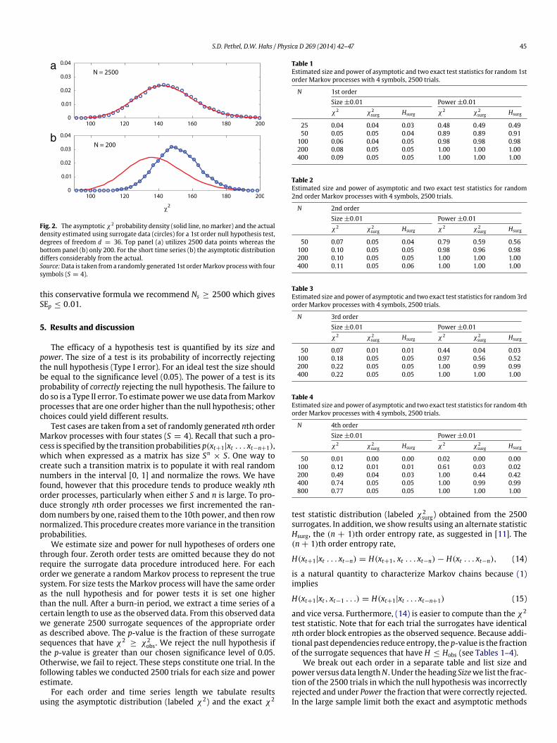
Fig. 2 shows the χ2 density computed in the asymptotic limitoverlaid with the density estimated from 20,000 surrogates of arandom Markov process of 4 states. The degrees of freedom arecalculated for a 1st order (n = 1, k = 2) null hypothesis test. Asdiscussed earlier, setting S = 4 and k = 2 gives Sk−1(S − 1)2 =

4·32= 36 degrees of freedom. In the top panel (N = 2500) there is

a close agreement indicating that the surrogate data statistics be-have as expected in the asymptotic limit. The bottom panel usesthe same time series, but only the first 200 data points. The signif-icant disagreement between the actual density and the density inthe asymptotic limit illustrates the need for an exact test when thesample is small.

As stated earlier, the p-value is the fraction of surrogatesequences that have χ2 values greater than or equal to χ2

obs. Letp be the true p-value and let Ns be the number of surrogatesequences. The expected number of sequences with χ2

≥ χ2obs is

Nsp with standard errorNsp(1 − p). Dividing by Ns gives SEp =

p(1 − p)/Ns as the standard error on the p-value estimate. Theworst case scenario is SEp = 1/

√4Ns when p = 1/4. Based on

S.D. Pethel, D.W. Hahs / Physica D 269 (2014) 42–47 45

a

b

Fig. 2. The asymptotic χ2 probability density (solid line, nomarker) and the actualdensity estimated using surrogate data (circles) for a 1st order null hypothesis test,degrees of freedom d = 36. Top panel (a) utilizes 2500 data points whereas thebottom panel (b) only 200. For the short time series (b) the asymptotic distributiondiffers considerably from the actual.Source:Data is taken froma randomly generated 1st orderMarkov processwith foursymbols (S = 4).

this conservative formula we recommend Ns ≥ 2500 which givesSEp ≤ 0.01.

5. Results and discussion

The efficacy of a hypothesis test is quantified by its size andpower. The size of a test is its probability of incorrectly rejectingthe null hypothesis (Type I error). For an ideal test the size shouldbe equal to the significance level (0.05). The power of a test is itsprobability of correctly rejecting the null hypothesis. The failure todo so is a Type II error. To estimate powerwe use data fromMarkovprocesses that are one order higher than the null hypothesis; otherchoices could yield different results.

Test cases are taken from a set of randomly generated nth orderMarkov processes with four states (S = 4). Recall that such a pro-cess is specified by the transition probabilities p(xt+1|xt . . . xt−n+1),which when expressed as a matrix has size Sn × S. One way tocreate such a transition matrix is to populate it with real randomnumbers in the interval [0, 1] and normalize the rows. We havefound, however that this procedure tends to produce weakly nthorder processes, particularly when either S and n is large. To pro-duce strongly nth order processes we first incremented the ran-domnumbers by one, raised them to the 10th power, and then rownormalized. This procedure creates more variance in the transitionprobabilities.

We estimate size and power for null hypotheses of orders onethrough four. Zeroth order tests are omitted because they do notrequire the surrogate data procedure introduced here. For eachorder we generate a randomMarkov process to represent the truesystem. For size tests the Markov process will have the same orderas the null hypothesis and for power tests it is set one higherthan the null. After a burn-in period, we extract a time series of acertain length to use as the observed data. From this observed datawe generate 2500 surrogate sequences of the appropriate orderas described above. The p-value is the fraction of these surrogatesequences that have χ2

≥ χ2obs. We reject the null hypothesis if

the p-value is greater than our chosen significance level of 0.05.Otherwise, we fail to reject. These steps constitute one trial. In thefollowing tables we conducted 2500 trials for each size and powerestimate.

For each order and time series length we tabulate resultsusing the asymptotic distribution (labeled χ2) and the exact χ2

Table 1Estimated size and power of asymptotic and two exact test statistics for random 1storder Markov processes with 4 symbols, 2500 trials.

N 1st orderSize ±0.01 Power ±0.01χ2 χ2

surg Hsurg χ2 χ2surg Hsurg

25 0.04 0.04 0.03 0.48 0.49 0.4950 0.05 0.05 0.04 0.89 0.89 0.91

100 0.06 0.04 0.05 0.98 0.98 0.98200 0.08 0.05 0.05 1.00 1.00 1.00400 0.09 0.05 0.05 1.00 1.00 1.00

Table 2Estimated size and power of asymptotic and two exact test statistics for random2nd order Markov processes with 4 symbols, 2500 trials.

N 2nd orderSize ±0.01 Power ±0.01χ2 χ2

surg Hsurg χ2 χ2surg Hsurg

50 0.07 0.05 0.04 0.79 0.59 0.56100 0.10 0.05 0.05 0.98 0.96 0.98200 0.10 0.05 0.05 1.00 1.00 1.00400 0.11 0.05 0.06 1.00 1.00 1.00

Table 3Estimated size and power of asymptotic and two exact test statistics for random3rdorder Markov processes with 4 symbols, 2500 trials.

N 3rd orderSize ±0.01 Power ±0.01χ2 χ2

surg Hsurg χ2 χ2surg Hsurg

50 0.07 0.01 0.01 0.44 0.04 0.03100 0.18 0.05 0.05 0.97 0.56 0.52200 0.22 0.05 0.05 1.00 0.99 0.99400 0.22 0.05 0.05 1.00 1.00 1.00

Table 4Estimated size and power of asymptotic and two exact test statistics for random4thorder Markov processes with 4 symbols, 2500 trials.

N 4th orderSize ±0.01 Power ±0.01χ2 χ2

surg Hsurg χ2 χ2surg Hsurg

50 0.01 0.00 0.00 0.02 0.00 0.00100 0.12 0.01 0.01 0.61 0.03 0.02200 0.49 0.04 0.03 1.00 0.44 0.42400 0.74 0.05 0.05 1.00 0.99 0.99800 0.77 0.05 0.05 1.00 1.00 1.00

test statistic distribution (labeled χ2surg) obtained from the 2500

surrogates. In addition, we show results using an alternate statisticHsurg, the (n + 1)th order entropy rate, as suggested in [11]. The(n + 1)th order entropy rate,

H(xt+1|xt . . . xt−n) = H(xt+1, xt . . . xt−n) − H(xt . . . xt−n), (14)

is a natural quantity to characterize Markov chains because (1)implies

H(xt+1|xt , xt−1 . . .) = H(xt+1|xt . . . xt−n+1) (15)

and vice versa. Furthermore, (14) is easier to compute than the χ2

test statistic. Note that for each trial the surrogates have identicalnth order block entropies as the observed sequence. Because addi-tional past dependencies reduce entropy, the p-value is the fractionof the surrogate sequences that have H ≤ Hobs (see Tables 1–4).

We break out each order in a separate table and list size andpower versus data lengthN . Under the heading Sizewe list the frac-tion of the 2500 trials in which the null hypothesis was incorrectlyrejected and under Power the fraction that were correctly rejected.In the large sample limit both the exact and asymptotic methods

46 S.D. Pethel, D.W. Hahs / Physica D 269 (2014) 42–47

Table 5Occurrence of wet and dry days classified by rainfall occurrence on the threepreceding days.Source: Data taken from the 27 Dec–Jan–Feb periods between 1950 and 1977 at TelAviv.

Preceding days Actual day Relative frequencyof wet days

Third Second First Wet Dry Total

– – – 716 1752 2468 0.290– – Wet 436 280 716 0.609– – Dry 280 1471 1751 0.160– Wet Wet 262 174 436 0.601– Dry Wet 174 106 280 0.621– Wet Dry 64 216 280 0.229– Dry Dry 216 1254 1470 0.147Wet Wet Wet 148 114 262 0.565Dry Wet Wet 114 60 174 0.655Wet Dry Wet 43 21 64 0.672Dry Dry Wet 131 85 216 0.607Wet Wet Dry 37 137 174 0.213Dry Wet Dry 27 79 106 0.255Wet Dry Dry 60 155 215 0.279Dry Dry Dry 156 1089 1254 0.124

should approach a size equal to the significance level (0.05) anda power of 1. The exact test is quite efficient; as few as 100 datapoints are needed for 1st and 2nd order tests, 200 for 3rd order, and400 for 4th order. The asymptotic method is very slow to attain theideal size even for the 1st order test (106 sample size, not shown).For higher order tests we do not recommend the use of the χ2 dis-tribution. There is no detectable difference between using the en-tropy rate as a test statistic and χ2. As entropy rate is a simplerquantity to calculate, we recommend its use over χ2; equivalently,and even simpler, would be to use the (n + 1)th block entropy.

Compared to the asymptotic χ2 test, the exact test is muchslower; each step of Whittle’s algorithm requires the computationof the determinant of the transition matrix. Considering that thetransition matrix changes in only one entry at each step there ispotential to improve the efficiency over our naive implementa-tion. Even without such optimizations, it is well within a desktopcomputer’s ability to generate many thousands of surrogate se-quences in minutes. Because each surrogate is generated indepen-dently, parallelization is straightforward. Each of our table entrieswas computed using 2500 trials with 2500 surrogates per trial, to-taling 6.25 million surrogates per table entry.

6. Application to real world data

Having validated the exact test using synthetic data, in thissection we will look at a real world application involving rainfalldata from Tel Aviv. This is a well-known data set whose Markovproperties were first studied by Gabriel and Neumann in 1962[15]. The data as originally prepared consisted of 27winter periods(December–January–February) with each day classified as eitherwet or dry. Based on the statistics of wet and dry spells the authorsconcluded that a first order Markov chain adequately models thedata. Later analysis using AIC indicates a second order chain shouldbe used [16], whereas BIC estimates the order at one [8].

Applying our Markov order significance test to this datapresents two challenges. The first barrier is that the data only existsas a table of transition counts. For hypothesis testing we needthe original time series, which in this case is the sequence of wetand dry days for each of the 27 winters between 1923 and 1950.Unable to find this data elsewhere, we chose instead to use TelAviv precipitation data between the years 1950 and 1977, whichis available in online databases [17]. We classified a day as wetif there were any precipitation recorded for that day. The secondproblem is that the data is not a single time series, but 27 disjoint

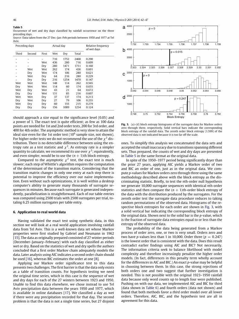
Fig. 3. (a)–(d) block entropy histograms of the surrogate data for Markov orderszero through three, respectively. Solid vertical bars indicate the correspondingblock entropy of the rainfall data. The zeroth order block entropy (1.599) of theobserved data is not indicated because it is too far off the scale.

ones. To simplify this analysis we concatenated the data sets andaccepted the small inaccuracy due to transitions spanning differentsets. Thus prepared, the counts of wet and dry days are presentedin Table 5 in the same format as the original data.

In spite of the 1950–1977 period being significantly dryer thanthe prior 27 years, applying AIC yields a Markov order of twoand BIC an order of one, just as in the original data. We com-pute p-values forMarkov orders zero through three using the samemethodology described above with the block entropy as the dis-criminating statistic. Briefly, to test the nth-order null hypothesiswe generate 10,000 surrogate sequences with identical nth-orderstatistics and then compare the (n + 1)th-order block entropy ofthe data with the distribution produced by the surrogates. For thezeroth order test the surrogate data procedure reduces to takingrandom permutations of the observed data. Histograms of the re-spective block entropies for each order are shown in Fig. 3, witha solid vertical bar indicating the corresponding block entropy ofthe original data. Shown next to the solid bar is the p-value, whichis the fraction of surrogate data entropies equal to or less than theentropy of the observed data.

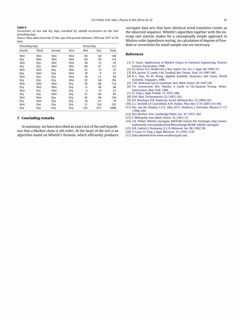
The probability of the data being generated from a Markovprocess of order zero, one, or two is very small. Orders zero andtwo have p-values less than 1 in 10,000. Order three (p = 0.247)is the lowest order that is consistent with the data. Does this resultcontradict earlier findings using AIC and BIC? Not necessarily.The information criteria seek to balance likelihood with modelcomplexity and therefore increasingly penalize the higher ordermodels. (In fact, differences in this penalty term wholly accountfor the differences in AIC and BIC.) An exact p-valuemay be helpfulin choosing between them. In this case, the strong rejections ofboth orders one and two suggest that further investigation isneeded. This is not possible with the original 1923–1950 rainfalldata because only word counts up to length four were published.Pushing on with our data, we implemented AIC and BIC for third(data shown in Table 6) and fourth orders (data not shown) andfound that both methods favor a third order model over all lowerorders. Therefore, AIC, BIC, and the hypothesis test are all inagreement for this data.

S.D. Pethel, D.W. Hahs / Physica D 269 (2014) 42–47 47

Table 6Occurrence of wet and dry days classified by rainfall occurrence on the fourpreceding days.Source: Data taken from the 27 Dec–Jan–Feb periods between 1950 and 1977 at TelAviv.

Preceding days Actual dayFourth Third Second First Wet Dry Total

Wet Wet Wet Wet 84 64 148Dry Wet Wet Wet 64 50 114Wet Dry Wet Wet 30 13 43Dry Dry Wet Wet 84 47 131Wet Wet Dry Wet 25 12 37Dry Wet Dry Wet 18 9 27Wet Dry Dry Wet 39 21 60Dry Dry Dry Wet 92 64 156Wet Wet Wet Dry 26 88 114Dry Wet Wet Dry 11 49 60Wet Dry Wet Dry 6 15 21Dry Dry Wet Dry 21 64 85Wet Wet Dry Dry 42 94 136Dry Wet Dry Dry 18 61 79Wet Dry Dry Dry 31 124 155Dry Dry Dry Dry 125 973 1098

7. Concluding remarks

In summary, we have described an exact test of the null hypoth-esis that a Markov chain is nth order. At the heart of the test is analgorithm based on Whittle’s formula, which efficiently produces

surrogate data sets that have identical word transition counts asthe observed sequence. Whittle’s algorithm together with the en-tropy rate statistic makes for a conceptually simple approach toMarkov order hypothesis testing; no calculation of degrees of free-dom or corrections for small sample size are necessary.

References

[1] A. Tamir, Applications of Markov Chains in Chemical Engineering, ElsevierScience, Amsterdam, 1998.

[2] P.J. Avery, D.A. Henderson, J. Roy. Statist. Soc. Ser. C-Appl. 48 (1999) 53.[3] R.A. Jarrow, D. Lando, S.M. Turnbull, Rev. Financ. Stud. 10 (1997) 481.[4] B.-L. Hao, W.-M. Zheng, Applied Symbolic Dynamics and Chaos, World

Scientific, Singapore, 1998.[5] T.W. Anderson, Leo A. Goodman, Ann. Math. Statist. 28 (1957) 89.[6] P.E. Greenwood, M.S. Nikulin, A Guide to Chi-Squared Testing, Wiley-

Interscience, New York, 1996.[7] H. Tong, J. Appl. Probab. 12 (1975) 488.[8] R.W. Katz, Technometrics 23 (1981) 243.[9] K.P. Burnham, D.R. Anderson, Sociol. Methods Res. 33 (2004) 261.

[10] C.C. Strelioff, J.P. Crutchfield, A.W. Hubler, Phys. Rev. E 76 (2007) 011106.[11] M.J. van der Heyden, C.G.C. Diks, B.P.T. Hoekstra, J. DeGoede, Physica D 117

(1998) 299.[12] M.S. Bartlett, Proc. Cambridge Philos. Soc. 47 (1951) 362.[13] P. Billingsley, Ann. Math. Statist. 32 (1961) 12.[14] S.D. Pethel, Whittle Surrogate, MATLAB Central File Exchange. http://www.

mathworks.com/matlabcentral/fileexchange/40188-whittle-surrogate.[15] K.R. Gabriel, J. Neumann, Q. J. R. Meteorol. Soc. 88 (1962) 90.[16] P. Gates, H. Tong, J. Appl. Meteorol. 15 (1976) 1145.[17] Data obtained from www.weatherspark.com.