evolutionary novelties and losses in geometric

ORIGINAL ARTICLE

doi:10.1111/j.1558-5646.2011.01244.x

EVOLUTIONARY NOVELTIES AND LOSSES INGEOMETRIC MORPHOMETRICS: A PRACTICALAPPROACH THROUGH HOMININ MOLARMORPHOLOGYAida Gomez-Robles,1,2,3 Anthony J. Olejniczak,4,5 Marıa Martinon-Torres,2 Leyre Prado-Simon,2

and Jose Marıa Bermudez de Castro2

1Konrad Lorenz Institute for Evolution and Cognition Research, Adolf Lorenz Gasse 2, 3422 Altenberg, Austria2Centro Nacional de Investigacion sobre la Evolucion Humana, Paseo de la Sierra de Atapuerca S/N, 09002 Burgos, Spain3E-mail: [email protected] of Anthropology, Stony Brook University, Stony Brook New York5Department of Human Evolution, Max Planck Institute for Evolutionary Anthropology, Deutscher Platz 6,

D-04103 Leipzig, Germany

Received August 23, 2010

Accepted January 21, 2011

Geometric morphometric techniques may offer a promising methodological approach to analyze evolutionary novelties in a

quantitative framework. Nevertheless, and despite continuous improvements to this methodology, the inclusion of novel features

in these studies presents some difficulties. In the present study, different methods to explicitly include novel traits in geometric

morphometric analyses are compared, including homology-free approaches, landmark-based approaches, and combinations of

both techniques. The two-dimensional occlusal morphology of the lower second molar in multiple hominin species was chosen to

evaluate these methods, as an example of an anatomical structure including one novelty: a distal fifth cusp is present in earlier

hominins, and notably absent in many later Homo species. Results reveal that different approaches provide different results,

highlighting that the design of the conformations of landmarks has a high impact on the inferred conclusions. Among diverse

methods, a combined approach including landmarks, sliding semilandmarks, and only one landmark related to the studied novelty

(an indicator of its absence or presence and of its size, when present), was able to directly discern structures with and without

the novel feature, circumventing some of the methodological difficulties associated with these traits. This study demonstrates

the ability of geometric morphometric techniques to investigate evolutionary novelties and explores the implications of different

methods, providing a reference context for future studies.

KEY WORDS: Discrete characters, homology, innovation, landmarks, morphological evolution, semilandmarks.

The evolution of phenotype often includes the novel gain or loss

of features, structures that are neither homologous to any an-

cestral structure nor equivalent to another structure in the same

organism (Muller and Wagner 1991). Evolutionary novelties de-

fined in this way are equivalent to neomorphic characters (Sereno

2007), the character states of which are limited to “present” or

“absent.” An important amount of work has been published as

to the developmental mechanisms underlying evolutionary nov-

elties (e.g., Jernvall 2000; Salazar-Ciudad 2006), especially from

a theoretical point of view (e.g., Love 2003; Muller and Newman

2005; Pigliucci 2008). Nonetheless, practical methodological ap-

proaches to novel traits tend to be restricted to categorical and

qualitative frameworks. Although suitable for cladistic analyses,

scoring of discrete traits does not allow for the recognition of

1 7 7 2C© 2011 The Author(s). Evolution C© 2011 The Society for the Study of Evolution.Evolution 65-6: 1772–1790

EVOLUTIONARY NOVELTIES IN GEOMETRIC MORPHOMETRICS

intermediate stages, for the measurement of degrees of proximity

or similarity, or for the prediction of hypothetical extremes (Roth

and Mercer 2000). These are actually the matters where quanti-

tative approaches provide an appropriate framework. As classic

morphometric methods are generally unsuitable to analyze novel

features (because they are unable to recover the presence or ab-

sence of discrete traits by means of traditional caliper measure-

ments), modern geometric morphometric techniques can offer a

promising alternative tool to study these traits.

Geometric morphometric methods, which are employed with

increasing frequency to describe morphological change in biolog-

ical structures (Adams et al. 2004), provide conceptual and tech-

nical refinements in morphological characterizations and compar-

isons. Nonetheless, the inclusion of evolutionary novelties in these

analyses is still controversial (Roth and Mercer 2000; Adams et al.

2004; Klingenberg 2008a; Polly 2008a,b). Inclusion of novel fea-

tures in geometric morphometric studies is problematic because

these analyses are based on a set of landmarks that are, by defi-

nition, common to all of the individuals within the study sample

(Adams et al. 2004). Thus, the typical approach to the problem

of novelties in geometric morphometric studies has been to con-

sciously exclude landmarks that are not present in all individuals

studied, and analyzing those novelties by describing the extent

to which the configuration of the other landmarks (those that

are present in all the individuals) are reorganized as the novelty

appears.

A clear example of this approach can be found in the classic

analysis by Marcus and colleagues of mammalian skull mor-

phology (Marcus et al. 2000), which included only landmarks

that could be identified in most living mammalian orders. They

concluded that, regardless of extreme morphological diversity,

the measured differences are surprisingly low. Marcus and col-

leagues (2000) demonstrated that even extremely different shapes

can appear uniform if only landmarks that are identifiable in all

specimens in the sample are included. This example shows that

surprisingly small shape differences are to be expected when only

the parts that are common to all the studied specimens are taken

into geometric consideration.

For these reasons, “homology-free methods” (e.g.,

Klingenberg 2008a; Polly 2008a) have been proposed as use-

ful for characterizing structures that are not present in all the

individuals studied. These methods facilitate modeling the ori-

gin of novel features because they are not limited to biologically

homologous landmarks, rather they describe the phenotype by

using mathematical algorithms that place individual points at reg-

ularly specified intervals which may, or may not, fall on the same

homologous structure (Polly 2008a). Homology-free approaches,

some of which have been used long before the appearance of

landmark-based geometric morphometrics, include several meth-

ods, such as sliding semilandmarks (Bookstein 1997; Gunz et al.

2005), Fourier analysis (e.g., Frieß and Baylac 2003; Bailey and

Lynch 2005, in a paleoanthropological context), and eigenshape

analysis (Lohmann 1983; MacLeod 1999). Furthermore, some

homology-free methods have been developed recently to study

three-dimensional (3D) surfaces, such as eigensurface analysis

(Polly 2008a,b; Polly and MacLeod 2008) and some variations of

3D Fourier surface analyses by using spherical harmonics (Shen

et al. 2009).

Nevertheless, homology-free methods are under debate, and

it has been suggested that these approaches are not actually free

of the assumption of homology. Alternatively, the homology as-

sumption has been transferred to the mathematical algorithms

rather than to biological criteria (Klingenberg 2008a). Thus, a

landmark-based method to study novelties consisting of struc-

tures that are gained, lost, or duplicated during evolution has been

proposed. This approach involves a set of landmarks demarcating

the novel structure when present, and falling on the same anatom-

ical point where that structure would be if it is absent (Fig. 1;

see Klingenberg 2008a for further details). The method proposed

by Klingenberg (2008a) “requires an explicit interpretation of

the developmental and anatomical change that underlies the nov-

elty” because the landmarks studied are not strictly homologous.

In this light, different criteria for correspondence between land-

marks in different individuals can be used depending on the type

of study, and the term “homology” is not appropriately used in all

the contexts. In any case, some morphometricians have noted the

necessity of adjusting landmark configurations to the hypotheses

being tested (Oxnard and O’Higgins 2009), even if a functional

criterion of correspondence between landmarks is used in lieu of

an anatomical one. Theoretical studies have discussed the utility

Figure 1. A schematic representation of the method of using a set

of landmarks demarcating a structure when present and falling on

the same anatomical point when absent, for evolutionary novel-

ties consisting of a gain (from right to left) or loss (from left to

right) of (sub)structures. Modified after Klingenberg (2008a).

EVOLUTION JUNE 2011 1 7 7 3

AIDA GOMEZ-ROBLES ET AL.

of this method (Klingenberg 2008a; Oxnard and O’Higgins 2009),

but it has not been tested using actual morphometric data, neither

has it been explicitly compared to homology-free approaches. The

present study employs two-dimensional (2D) landmarks describ-

ing molar morphology in a broad sample of hominins to compare

these methods.

The lower second molar of different hominin species has been

chosen to study evolutionary novelties in a geometric morphome-

tric framework because this is the key tooth in the molar series for

studying the variability in the number of cusps (Scott and Turner

1997). This molar has four main cusps in all hominin species: pro-

toconid (c1), metaconid (c2), hypoconid (c3), and entoconid (c4).

The Australopithecus, Paranthropus, and early Homo specimens

also possess a fifth cusp located at the distal part of the molar,

called hypoconulid or c5 (Fig. 2). However, in later Homo species

(particularly H. sapiens) c5 is often absent, evincing a morphology

consisting of four subequal cusps (Scott and Turner 1997; Bailey

2002; Martinon-Torres 2006). Nonetheless, later Homo species

have intraspecific variation in this feature, with some specimens

showing the primitive five-cusp configuration (Scott and Turner

1997). Although the size of this cusp tends to decrease from early

to later hominins, under a determinate size threshold this cusp

does not appear (Turner et al. 1991; Jernvall 2000).

The existence (or lack) of different cusps in mammalian mo-

lars and premolars is determined by the formation of secondary

enamel knots (Jernvall et al. 1994), which appear at the locations

of the future cusp tips (Jernvall and Jung 2000). Secondary enamel

knots, formed during the early development of postcanine teeth,

are the first signs of cusps and different activator and inhibitor sig-

nals help to establish the onset of species-specific cusp patterns

(Keranen et al. 1998; Jernvall and Jung 2000). The early determi-

nation of the tooth shape during the ontogenetic development of

Figure 2. Representation of the landmarks and semilandmarks used in each model. Big circles with black edges correspond to landmarks

(numbers in black types). Small white circles correspond to semilandmarks (numbers in white types). Note that in all the models including

landmarks related to the c5 (models “Land”, “c5 Proc Dist”, “c5 BE”, and “Beginning c5”), these landmarks (#8, #9 and #10) fall over the

distal part of the outline in the four-cusped molar located to the right. Numbers of landmarks are the same as those in Table 2. Note also

that models “c5 Proc Dist” and “c5 BE” employ exactly the same configuration of landmarks and semilandmarks. Orientation of molars:

buccal–top; lingual–bottom, mesial–left; distal–right.

1 7 7 4 EVOLUTION JUNE 2011


teeth demonstrates that the presence or absence of different cusps

is a true evolutionary novelty (or loss), established early during

odontogenesis. In fact, the patterning cascade mode of cusp de-

velopment proposed by Jernvall and colleagues (e.g., Jernvall and

Jung 2000) is a conceptual bridge through which the evolution-

ary gain or loss of cusps can be linked to underlying ontogenetic

mechanisms from an EvoDevo perspective.

The study presented here explores different ways to analyze

evolutionary novelties in a quantitative framework and proposes

multiple methods to include the repeated gain and loss of den-

tal cusps in a landmark- and/or semilandmark-based geometric

morphometric analysis. Some statistical properties of these meth-

ods and their results are compared, evaluating their ability to

correctly address taxonomic assignment and phylogenetic recon-

struction when analyzing the morphology of the hominin lower

second molar.

Materials and MethodsMATERIALS

One hundred and twenty-nine lower second molars of the

hominin genera Australopithecus, Paranthropus, and Homo were

studied. A complete list of specimens is given in Table 1. The tax-

onomic assignment of the individuals follows criteria previously

discussed by Gomez-Robles and colleagues (Gomez-Robles

et al. 2007, 2008).

All analyses were carried out using photographs of the oc-

clusal surface of the molars. A Nikon D1H digital camera (Tokyo,

Table 1. Specimens included in the analyses. The number of mo-

lars with four or five cusps within each species is specified.

Species Total Four cusps Five cusps

A. afarensis 9 0 9A. africanus 5 0 5Paranthropus sp.1 9 0 9H. habilis s. l.2 4 0 4H. ergaster3 6 0 6H. erectus4 11 0 11H. antecessor 3 0 3H. heidelbergensis5 24 3 21H. neanderthalensis6 18 0 18H. sapiens7 40 29 11

Total 129 32 97

1Including P. robustus and P. boisei.2Including H. habilis and H. rudolfensis.3Including also Lower and Middle Pleistocene individuals from Africa and

Georgia.4Pliocene, Lower, and Middle Pleistocene individuals from Eastern Asia.5European Middle Pleistocene individuals.6European Upper Pleistocene individuals.7Upper Pleistocene and contemporary individuals.

Japan) fitted with an A/F Micro-Nikkor 105 mm, f/2.8D, was used

to collect the images. Attachment to a Kaiser Copy Stand Kit RS-

1 ensured correct positioning of the camera, and the depth of

field was adjusted to f/32. Each tooth was positioned so that the

cemento-enamel junction and the occlusal surface were parallel to

the lens of the camera (Wood and Abbott 1983; Wood and Engle-

man 1988). Further details regarding the positioning of teeth and

the error introduced during the photography process are described

by Gomez-Robles et al. (2008). Right molars were studied when

both antimeres were present, and left molars were mirror-imaged

when the right molar was absent, broken, or the identification of

landmarks was unclear.

GEOMETRIC MORPHOMETRIC METHODS

Landmark-based geometric morphometric approaches compare

the location of x- and y-coordinates of homologous landmarks

located at some relevant points of the studied structures (Zelditch

et al. 2004). Procrustes superimposition (Rohlf and Slice 1990;

Bookstein 1991) extracts all of the geometric information re-

maining in the sample after translating, scaling, and rotating the

landmark configurations until the distances between correspond-

ing landmarks (Procrustes residuals) are minimized following a

least squares criterion.

The thin plate spline method (Bookstein 1989, 1991) uses

the bending energy, which is a measure of the degree of local-

ization of a deformation, to obtain a new set of variables called

partial warps scores. These variables indicate how the principal

warps (the set of shape features that can be combined together to

yield every possible nonuniform shape change from the starting

conformation) must be combined in the x and y direction to obtain

a particular target configuration (Bookstein 1989, 1991, 1996a).

The principal component analysis of the partial warp scores is

called relative warp analysis (Bookstein 1991), and it captures

the main patterns of morphological variation within the sample

in the first few principal components or relative warps (Frieß

2003). If no weighting according to the bending energy is used,

and the uniform component of the shape variation (with equal

effects throughout the complete structure) is included (Rohlf and

Marcus 1993), the relative warps are the same as the principal

components derived from the covariance matrix of the Procrustes

residuals measured between the mean shape of the sample (con-

sensus) and each specimen (Mitteroecker and Gunz 2009).

Thin plate spline also provides a visual representation of

the morphological variation when one specimen is morphed into

another by recording changes in the relative position of the land-

marks and representing them as TPS-grids. The changes in the

areas between the landmarks are interpolated so that there is a

minimal abrupt change or, in other words, the amount of bending

energy that is required to convert one conformation to the other

is minimized (Mitteroecker and Gunz 2009).



Sliding semilandmarks are useful for describing the morphol-

ogy of structures without landmarks, such as curves or outlines

(Bookstein 1996b, 1997; Bookstein et al. 1999). Because semi-

landmarks do not depend upon a precise location along the curve

or outline, they are slid along a tangent line to the curve (and

the component of the difference that lies along this tangent is

removed; see Perez et al. 2006) until their final location mini-

mizes either the Procrustes distance between the reference and

the target (e.g., Martinon-Torres et al. 2006; Gomez-Robles et al.

2007, 2008), or the bending energy (Bookstein 1997; Bookstein

et al. 1999, 2003; Gunz et al. 2005). Use of either method implies

different assumptions with respect to the part of the shape change

that is recovered (Gunz et al. 2005; Bastir et al. 2006), and they

provide different results, as demonstrated by Perez and colleagues

(Perez et al. 2006).

GEOMETRIC MODELS

Occlusal photographs were used to evaluate the six different geo-

metric models represented in Figure 2 (see below), corresponding

to different methods proposed to evaluate the presence of evolu-

tionary novelties. In molars with a sixth cusp (a developmentally

secondary cusp that may appear lingually to the c5, Keene 1994),

both c5 and c6 were considered together as a “c5-c6 complex”

(referred to as c5 throughout the text). This method gives more

importance to the primary cusps, measuring the c5 as the entire

area that falls between the developmentally primary c3 and c4

(Keene 1982, 1991). All the models including landmarks used

anatomical points located at the tips of the main cusps, at the in-

tersection of the main grooves, and at the intersection of the main

grooves with the dental outline (see Table 2 for definition of the

landmarks). For the models using semilandmarks, 39 equidistant

points were drawn along the dental outline using the tool “Out-

line” in the TpsDig2 software (Rohlf 2005). Although TpsDig2

software does not yield perfectly evenly spaced semilandmarks,

their position is modified later when applying the sliding mecha-

nisms, so their initial location is not relevant to the final results.

The first model, referred to in tables and figures as “Semi”,

consisted of a set of 39 sliding semilandmarks describing only the

shape of the molar perimeter as an example of a homology-free

approach. One landmark was located at the hypothetical inter-

section of the prolongation of the central groove with the mesial

outline as the starting point, and the semilandmarks were then slid

using the criterion of minimization of Procrustes distances.

The second model (“Land”) consisted of a set of 17 land-

marks (Biggerstaff 1969), including three points demarcating the

c5. These three landmarks were located at the three vertices of

the c5 (the intersection of the central groove with the disto-bucal

groove, the intersection of the disto-bucal groove with the molar

outline, and the intersection of the prolongation of the central

groove with the distal outline, Fig. 2 and Table 2) in molars with

five cusps, and they fell on the same anatomical point, located at

the intersection of the central groove with the distal outline, in

molars with four cusps. No semilandmarks were used in this case,

to test the extent to which dental morphology can be recovered

only by landmarks, avoiding methodological problems related to

the use of semilandmarks (Bruner 2008). Nevertheless, five out-

line landmarks with at least one deficient coordinate, (Bookstein

1991) were located throughout the dental periphery, following

Biggerstaff (1969).

The third model (“Semi+Land no c5”) followed the clas-

sic approach of excluding all landmarks that are not present in

all individuals, ultimately including only seven landmarks, none

of which was related to the c5, and 39 sliding semilandmarks.

Although no landmark explicitly related to the c5 was included

in this model, the extent to which the other landmarks are reor-

ganized depending on whether this cusp is present or absent is

presumably recovered in the landmark configuration. As above,

semilandmarks were slid by minimizing the Procrustes distances

between the curve on the consensus and each individual in the

sample.

Next, 10 landmarks, including the three which demarcate the

c5, and 39 sliding semilandmarks were employed as an attempt

to include all available morphological information. In this case,

the combination of both landmarks and semilandmarks causes

abrupt changes in the TPS-grids, with creases located at areas of

high morphological variation (Bookstein 2000). Therefore, with

the aim of minimizing this change and having a smooth variation

in the TPS-grids, this set of landmarks and semilandmarks was

studied by sliding the semilandmarks following the two different

criteria: the minimization of Procrustes distances as the fourth

model (“c5 Proc Dist”), and the minimization of bending energy

as the fifth model (“c5 BE”).

Finally, a simplification of the method of demarcating the c5

was created by including eight landmarks and 39 sliding semi-

landmarks in the last model, referred to as “Beginning c5.” The

set of eight landmarks included only one point related to the c5,

which is located at the intersection of the central groove with the

disto-buccal groove (Fig. 2) and can be considered the “geometric

beginning” of the c5. This landmark is slid toward the dental pe-

riphery as the c5 reduces in size, falling at the intersection of the

central groove with the distal outline in molars with four cusps.

All landmarks and semilandmarks were digitized by one of

us (AG-R) using TpsDig2 software (Rohlf 2005). To avoid bias

related to digitization errors, all landmarks and semilandmarks

were digitized only once for each specimen, and those landmarks

that were not included in a particular model were removed using

TpsUtil software (Rohlf 1998a).

Although many different geometric models can be designed

to describe the analyzed morphologies, the six models employed

here have been chosen ad hoc to recover some of the most relevant



Table 2. Definition of the landmarks.

Landmark Definition Type1 Model/s2

1 Tip of the mesiobuccal cusp or protoconid (c1) 2 LandSemi+Land no c5c5 Proc Distc5 BEBeginning c5

2 Tip of the mesiolingual cusp or metaconid (c2) 2 LandSemi+Land no c5c5 Proc Distc5 BEBeginning c5

3 Tip of the distobuccal cusp or hypoconid (c3) 2 LandSemi+Land no c5c5 Proc Distc5 BEBeginning c5

4 Tip of the distolingual cusp or entoconid (c4) 2 LandSemi+Land no c5c5 Proc Distc5 BEBeginning c5

5 Center of the mesial fovea 2 LandSemi+Land no c5c5 Proc Distc5 BEBeginning c5

6 Point where the central groove is crossed bythe mesiobuccal groove

1 LandSemi+Land no c5c5 Proc Distc5 BEBeginning c5

7 Point where the central groove is crossed bythe lingual groove

1 LandSemi+Land no c5c5 Proc Distc5 BEBeginning c5

8 Point where the central groove is intersected bythe distobuccal groove (beginning of the c5).In four-cusped molars, point where thedental outline is intersected by the distalprolongation of the central groove

1 Landc5 Proc Distc5 BEBeginning c5

9 Point where the dental outline is intersected bythe distobuccal groove. In four-cuspedmolars, point where the dental outline isintersected by the distal prolongation of thecentral groove

1–33 Landc5 Proc Distc5 BE

10 Point where the dental outline is intersected bythe distal prolongation of the central groove

1–33 Landc5 Proc Distc5 BE

Continued.



Table 2. Continued.

Landmark Definition Type1 Model/s2

11 Point where the dental outline is intersected bythe mesiobuccal groove

1–33 Land

12 Point where the dental outline is intersected bythe lingual groove

1–33 Land

13 The most mesial point of the occlusal outlineopposite the mesial fovea

3 Land

14 Inflection point between the buccal margin andthe mesial margin

3 Land

15 Inflection point between the buccal margin andthe distal margin

3 Land

16 Inflection point between the lingual margin andthe mesial margin

3 Land

17 Inflection point between the lingual margin andthe distal margin

3 Land

39 equispaced sliding semilandmarks locatedat the dental outline

SemiSemi+Land no c5c5 Proc Distc5 BEBeginning c5

1Type 1 landmark=landmarks located at the juxtaposition of tissues or structures; Type 2 landmarks=landmarks located at local minima or maxima of

curvature; Type 3 landmarks=extreme points in various dimensions that have at least one deficient coordinate (Bookstein 1991).2Models where the previously defined landmarks have been used.3The location of these landmarks at the juxtaposition of structures makes them similar to type 1 landmarks, but one of these structures is the dental

periphery and, therefore, they have some of the same limitations as type 3 landmarks.

and commonly used data sampling strategies. The model based

only on landmarks (“Land”) includes basically all the true land-

marks that can be identified in occlusal images of human molars,

whereas the model based only on semilandmarks (“Semi”) meets

the aim of recovering only morphological information indepen-

dent of homologous landmarks. Some works have been published

as to the smallest number of semilandmarks needed to sample a

curve to a specified degree of accuracy (MacLeod 1999; Skin-

ner et al. 2009), but determining this number of semilandmarks

is not the aim of the present work. Therefore, the number of 39

outline points has been chosen based on similar studies of dental

morphology (e.g., Perez et al. 2006; Wood et al. 2007). Further-

more, although the comparison of the cemento-enamel junction

(or cervix curve) might be considered more appropriate in terms

of homology, the aim of comparing the occlusal outline is em-

ploying a nonhomologous structure that, in any case, has been

demonstrated to differentiate closely related species and popula-

tions (e.g., Polly 2003; Bailey and Lynch 2005; Xing et al. 2009).

The four remaining models combine the information coming from

homology-based and homology-free methods by: excluding in-

formation related to the analyzed novelty (“Semi+Land no c5”);

including only one landmark related to the evolutionary novelty

(“Beginning c5”); and including all the homologous and nonho-

mologous information, but using different sliding mechanisms to

describe the nonhomologous part (“c5 Proc Dist” and “c5 BE”).

Although many variations of these models may be used, we con-

sider that the six employed ones are representative of the most im-

portant sampling strategies currently in use by most researchers.

The six different models employed to analyze evolutionary

novelties through landmark- and semilandmark-based geomet-

ric morphometrics have been evaluated by means of two sets of

methods. The first group of methods has been used to compare

the statistical properties of the geometric models. Alternatively,

the second group has been used with the practical aim to ex-

plore the ability of these models to correctly address the problems

of taxonomic assignment and phylogenetic reconstruction. Files

with landmark and semilandmark conformations used to carried

out these analyses are deposited at Dryad database and can be

found at http://dx.doi.org/10.5061/dryad.8478.

STATISTICAL ANALYSES

The amount of morphological variance measured when using

each model was calculated to evaluate whether some models

under- or overestimate the amount of variance when analyzing



the same morphological structure. Procrustes variance was

calculated by summing the eigenvalues corresponding to all the

PCs (Blackith and Reyment 1971) using routines for Math-

ematica 7.0 written by P. David Polly and available on line

(http://mypage.iu.edu/∼pdpolly/). In an opposite way to other

methods employed in this study, which analyze relative parame-

ters inherent to the different geometric models, Procrustes vari-

ance is an absolute measurement that is highly dependent upon the

number of landmarks. For this reason, variances corresponding

to different landmark configurations are not directly comparable.

Hence, this comparison was not based on total Procrustes variance

measured by each model, but on the variance differential with re-

spect to what would be expected for a determinate number of

landmarks and semilandmarks. Resampling methods with 1000

replications were used to measure how variance per landmark

and total Procrustes variance vary as the number of landmarks

increases from 5 up to 100 landmarks. As the number of land-

marks in these molars is limited to approximately 20 points, this

analysis was carried out using semilandmarks located at the dental

periphery as real landmarks. This way, there is no limitation in the

number of landmarks that can be evaluated. Procrustes variances

expected for a determined number of landmarks were compared

to actual variances measured when using each model.

Apart from the total amount of Procrustes variance, different

geometric models are also expected to differ in the distribution

of that variance. The distribution of variance was represented as

a scree plot depicting the percentage of morphological variance

explained by each PC after a relative warp analysis. Significant

differences in eigenvalue distributions were tested by comparing

the eigenvalue variance (EV) of 1000 bootstrapped samples in

the six models (e.g., Wagner 1984; Young 2006; Pavlicev et al.

2009). Because they are calculated from covariance matrices, EV

is scale-dependent, so eigenvalues were standardized by the total

shape variance (Young 2006). EV also depends upon the number

of traits (Pavlicev et al. 2009), but this dependency on size of

the matrices can be accounted for by using the relative EV (i.e.,

observed EV divided by the number of eigenvalues, minus one;

Pavlicev et al. 2009). Nevertheless, this measurement of variance

is affected by the presence of null eigenvalues (PCs that account

for almost no variance), so EV was calculated by using only

those PCs that account for 99% of total Procrustes variance of the

sample when using each model.

Similarities and differences between the morphological

changes recovered by the different models were evaluated by

means of multivariate and bivariate tests. The correlation of mul-

tivariate shapes recovered by each model was tested via pair-

wise two-block partial least squares analyses (2B-PLS, Rohlf and

Corti 2000) using MorphoJ software (Klingenberg 2008b). This

analysis uses a singular value decomposition to find correlated

pairs of linear combinations (singular vectors) of variables (Book-

stein 1991; Rohlf and Corti 2000; Bookstein et al. 2003), and it

maximizes the low-dimensional representation of between-block

covariance structure (Klingenberg 2008b). The RV coefficient

was used as a multivariate analogue of the squared correlation

(Escoufier 1973; Klingenberg 2009), and its significance was

tested via permutation tests for the null hypothesis of complete

independence between the two blocks with 1000 random per-

mutations of the sets of landmarks (Klingenberg 2009). The RV

coefficient is analogous to the correlation coefficient between two

variables because it represents the amount of covariation scaled

by the amounts of variation within the two sets of variables. How-

ever, this coefficient uses squared measures of variances and co-

variances, and is therefore more directly comparable to a squared

correlation coefficient (Klingenberg 2009). Additionally, correla-

tion coefficients among the first and second PCs obtained in the

relative warp analysis for the six models were calculated.

Relative warp analyses were employed not only as a previous

step in some of the aforementioned comparisons, but they were

also carried out to compare the distribution of individuals in the

morphospace when using the six different models. Graphical rep-

resentations of these analyses involved only the first and second

relative warps. TPS-grids corresponding to the extremes of the

first and second PCs were obtained from TpsRelw (Rohlf 1998b).

Finally, the relationship between the discrete change repre-

sented by the loss of the fifth cusp and continuous variation in

molar size and shape was also evaluated. Although it is true that

the complete sequence of reduction of the fifth cusp cannot be

observed in the hominin fossil record, this evolutionary change is

not completely discrete, but a reduction in both the total size of the

molar, and the absolute and relative size of the c5 (when present)

is observed in later Homo species (Turner et al. 1991; Martinon-

Torres 2006). The extent to which the continuous morphological

change recovered when excluding the landmarks related to the c5

(in the model “Semi+Land no c5”) can be explained by the total

size of the molars (recovered as the centroid size), the absolute

size of the c5, and the relative size of the c5, was tested with a

multivariate regression of the partial warp scores and the uniform

component on these three variables. This test was performed with

TpsRegr software (Rohlf 1998c).

TAXONOMIC AND PHYLOGENETIC ANALYSES

Taxonomic and phylogenetic analyses included only the species

with largest sample sizes (A. afarensis, H. erectus, H. heidelber-

gensis, H. neanderthalensis, and H. sapiens), which are also some

of the most commonly accepted hominin species. It has to be con-

ceded, however, that both taxonomy and phylogeny within the

human clade are vigorously debated and there is seldom agree-

ment between different authors. Hence, neither taxonomy nor

phylogeny can be considered to be an unequivocal reference con-

text in this study. Even though, both taxonomic distinction and



phylogenetic relationships among the five selected groups are

broadly accepted based not only on their skeletal morphology,

but also on their chronology and geographic location. These re-

lationships are closer between H. heidelbergensis (represented

by pre-Neanderthal European populations in this study, Arsuaga

et al. 1997) and H. neanderthalensis, and more distant between

the pre-Neanderthal–Neanderthal clade (or lineage) and H. sapi-

ens, these three species and H. erectus, and these four species and

A. afarensis.

A canonical variates analysis (CVA) was carried out to assess

the accuracy with which molars are correctly classified to each

species using each model, as a measurement of the suitability

of each model within a taxonomic framework. The number of

variables included in the CVA was reduced by using only the

first seven PCs. Percentages of correct assignments were cross-

validated by considering each specimen as unknown, and then

classifying it based on the remaining sample.

Phylogenetic utility of each method was evaluated by means

of a neighbor-joining (NJ) cluster analysis (Saitou and Nei 1987)

based on the matrix of Procrustes distances among the mean shape

of the different species when using each geometric model. This

approach has been used by several authors in a geometric morpho-

metric context (e.g., Polly 2001; Lockwood et al. 2004; Cardini

and Elton 2008; Harvati et al. 2010) because it uses distances

among taxa rather than character states, so it allows to make

phylogenetic inferences using shape as a character (Klingenberg

and Gidaszewski 2010). The NJ analysis was carried out with

PHYLIP software (Felsenstein 2005), and it used P. troglodytes

as outgroup (the mean shape of P. troglodytes was calculated from

a sample of 18 chimpanzee lower second molars analyzed under

the same six models explained above).

Mean shape comparisons among the three species with

largest sample sizes, (H. heidelbergensis, H. neanderthalensis,

and H. sapiens) are provided in tabular form. Permutation tests

with 1000 random permutations were used to evaluate the statis-

tical significance of mean shape differences in each model, and

Procrustes distances among the mean shape of the three species

obtained with the six models were compared. The IMP set of

software programs (Sheets 2001) was employed for these com-

parisons. A reference context was established (Gomez-Robles

2010) by measuring the Procrustes distances between the mean

shapes of the three species in six teeth that do not gain or lose

main cusps during their evolution (upper and lower first and

second premolars and upper and lower first molars; Scott and

Turner 1997). These distances are based on a set of landmarks

and sliding semilandmarks and, therefore, they have different

values than expected if they were based only on landmarks,

or only on semilandmarks. Nonetheless, they provide a refer-

ence against which to evaluate the results of the lower second

molar.

Figure 3. Procrustes variance versus number of landmarks. Top:

mean variance per landmark decreases as number of landmarks in-

creases. Middle: total Procrustes variance increases as landmarks

are added. Bottom: Total Procrustes variance versus number of

landmarks (same as previous plot) represented together with Pro-

crustes variances measured using the six described models.

ResultsSTATISTICAL PROPERTIES OF THE MODELS

Figure 3 (top) demonstrates that the variance per landmark de-

creases in datasets with more points because as points are added,

the shape gets smaller in the space because the sum of the squared

distances between the landmarks and the centroid is held equal to

1. However, the decreased variance per landmark is compensated

for by the higher number of landmarks, so total variance increases

as landmarks are added (Fig. 3, middle). Nonetheless, Figure 3

(bottom) shows that the increment in total variance as landmarks

are added is negligible when compared to the amount of variance



Figure 4. Scree plots corresponding to the relative warp analyses carried out for the six models. The x-axis represents the number of

PCs, and y-axis represents the percentage of variance explained by each PC. Eigenvalue variances are provided. Although the same scale

is used in the six cases to facilitate comparison, the number of PCs depends on the number of landmarks and semilandmarks included in

the model, and it is different in each case.

measured by the different models. The greatest variance differ-

ential with respect to what would be expected corresponds to

the second model (“Land”), and the least variance is found in

the model “Semi” (because this model is based only on semi-

landmarks, the Procrustes variance corresponds exactly with the

expected value). The other models have intermediate values, but

the amount of variance measured in the model “c5 BE” (minimiz-

ing bending energy to slide semilandmarks) is twice as high as the

variance in the model “c5 Proc Dist” (minimizing the Procrustes

distance), although exactly the same landmarks and semiland-

marks were used in both models.

As observed in the scree plots (Fig. 4), the distribution of

variance is also different in the six models. All the models in-

cluding the c5 have a leading PC accounting for more than 50%

of the total morphological variance of the sample. However, the

two models that do not include the c5 explicitly have a more

homogeneous distribution of variance, with the first few PCs ex-

plaining similar percentages of variance. Significant differences

in EV were found between all the models (F = 3582.25; P <

0.001). Post hoc tests show that these differences are significant

between each pair of models, with the only exception of the com-

parison between “Land” and “c5 Proc Dist” (F = 2.459; P =0.118). The highest EV corresponds to “c5 BE,” whereas lower

and very similar values were found for “Land” and “c5 Proc Dist.”

The two models that include no landmark related to the c5 have

the lowest EVs, with the lowest value corresponding to the model

“Semi+Land no c5.”

In Figure 5, the values of correlations between all the first

and all the second PCs in the six models are depicted. These cor-

relations are high between the model “Land” and all the models

including the c5. However, the model “Semi” has lower correla-

tions with all the other models (some of which are not significant)

and it has the highest correlation with “Semi+Land no c5.” The

model “Beginning c5” has high correlations with all the models

including the fifth cusp, whereas the model “Semi+Land no c5”

has only moderate correlations with the other models. The values

of the RV coefficients, which measure the squared correlation

among the multivariate shapes in the six models by using 2B-PLS

analyses, show similar results (Table 3), with values higher than

RV = 0.9 between most models including the c5. In the multivari-

ate case, all of the pairwise squared correlations are significant,

although the model “Semi” has low RV coefficients, especially

when compared with the model “Land.”

In the plots based on relative warp analyses (Fig. 6) of the

four models including the c5, a clear clustering of molars with four

versus five cusps can be identified, with an unoccupied area in the

morphospace between these groups. However, PCAs correspond-

ing to the models “Semi” and “Semi+Land no c5” do not show

such a separation, although trends can be identified for positive or

negative values in different species. Evolutionary change corre-

sponding to the loss of the c5 is clearly visualized in all the models,

with the exception of the model “Semi.” Such a change is also

visible in the model “Semi+Land no c5,” the TPS-grids of which

show the reorganization of the landmarks located adjacent to the

fith cusp. Both models that include the three landmarks demar-

cating the c5 and sliding semilandmarks show abrupt changes in

their TPS-grids, with creases located at areas of high morpholog-

ical variation. The first PC in the model “Semi” corresponds to an



Figure 5. Correlation among the first and second PCs for the six models. First PCs are represented at the lower left half of the table, and

second PCs, at the right upper half. The correlation coefficients are provided together with the scatter plots. ∗P < 0.05; ∗∗P < 0.01.

elongation of the mesio-distal axis of the molar that is observed in

Neanderthals, and which is difficult to visualize when landmarks

are also included in the model.

The multivariate regression carried out for the model

“Semi+Land no c5” on the centroid size (overall size of the

molars), absolute size of the c5, and relative size of the c5 show

that the three variables have significant predictive power of the

molar shape (Fig. 7). Overall molar size explains 9.37% of the

morphological variance, absolute size of the fifth cusp explains

13.22% of the morphological variance, and relative size of the

c5 explains 13.02% of the total morphological variance. The cor-

relation between the absolute and relative size of the c5 is r =0.908, so it is expected to find similar values in the multivariate

regression of partial warp scores on both variables.

TAXONOMY AND PHYLOGENY

The assignment tests based on the CVAs also show differ-

ent percentages of correctly assigned individuals, the highest

values corresponding to the model “Semi+Land no c5” (original

percentages), and to “Beginning c5” (cross-validated percentages,



Table 3. RV coefficients for the pairwise comparisons of the six geometric models by using two-block partial least squares analysis.

Semi Land Semi+Land no c5 c5 Proc Dist c5 BE Beginning c5

Semi 0.1641∗ 0.6205∗ 0.2049∗ 0.2222∗ 0.2725∗

Land 0.1641∗ 0.5886∗ 0.9848∗ 0.9431∗ 0.9107∗

Semi+Land no c5 0.6205∗ 0.5886∗ 0.6881∗ 0.4819∗ 0.8634∗

c5 Proc Dist 0.2049∗ 0.9848∗ 0.6881∗ 0.9525∗ 0.9268∗

c5 BE 0.2222∗ 0.9431∗ 0.4819∗ 0.9525∗ 0.6714∗

Beginning c5 0.2725∗ 0.9107∗ 0.8634∗ 0.9268∗ 0.6714∗

Highly significant multivariate squared correlations (P < 0.01) based on 1000 random permutations.

Figure 6. Relative warp analyses corresponding to the six studied models. The TPS-grids correspond to the morphological variants

located at the extreme of each PC within the range of variation of each particular model. Graphs are not to the same scale. Orientations

of molars represented as TPS-grids are the same as in Figure 2.



Figure 7. Morphological variants corresponding to the minimum

and maximum values of the multivariate regression of the partial

warp scores plus the uniform component on the centroid size (CS),

absolute area of the c5 (c5 abs), and relative area of the c5 (c5

rel). Absolute area of the c5 is measured in millimetre square.

Orientations of molars represented as TPS-grids are the same as

in Figures 2 and 6.

Table 4). Because these tests are based on the first seven PCs, and

the amount and percentage of variance accounted for these PCs

differ in each model, it may be reasonable to relate the highest

percentages of correct classification to the models with high-

est percentages of variance explained in those first seven PCs.

Nonetheless, the two models showing the best results in terms

of correctly classified molars (84.15% and 83.17%, when all five

species are considered together) correspond to the two models

with lowest percentages of variance explained by the PCs in-

cluded in the CVA (73.21% and 83.39%). The lowest values of

correct classification are found in the model “c5 BE” and in the

model “Semi,” which are the models with the largest amount of

variance explained by PC1 through PC7 (93.17% and 89.91%,

respectively).

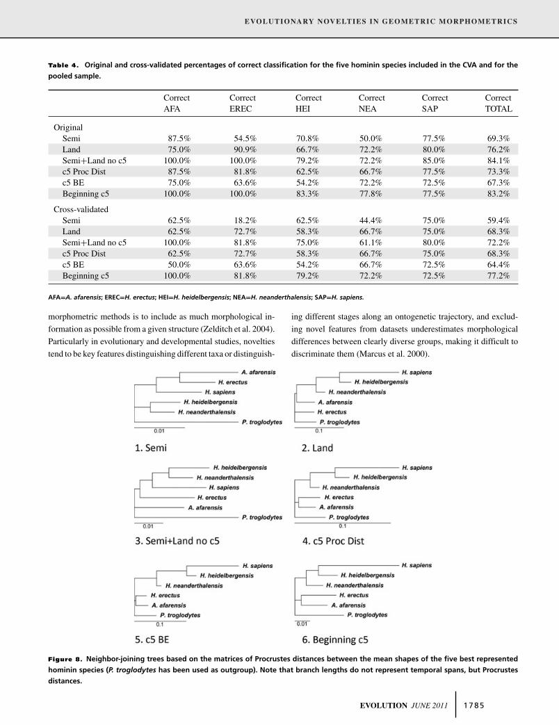
As for phylogenetic relationships inferred from lower second

molar morphology, only the model “Semi+Land no c5” recov-

ers the true hominin phylogeny to some degree (although the

recovered relationship of A. afarensis with Homo species is the

same than that of the outgroup). The model “Semi” clusters A.

afarensis and H. erectus with H. sapiens and separates H. hei-

delbergensis and H. neanderthalensis in a different group. The

model “Land” groups H. sapiens with H. heidelbergensis, these

two species with H. neanderthalensis, and these three species

with A. afarensis. The three models that include both semiland-

marks and landmarks (also those related to the c5) are not able to

recognize the closest relationship between pre-Neanderthals and

Neanderthals. Instead, these three models (“c5 Proc Dist,” “c5

BE,” and “Beginning c5”) give rise to two clusters: one formed

by the three latest Homo species (H. sapiens, H. heidelbergensis,

and H. neanderthalensis), and another one formed by H. erectus

and A. afarensis (Fig. 8).

In spite of the results of the NJ analysis, all the models but

“Semi+Land no c5” recover the expected lower Procrustes dis-

tance between H. heidelbergensis and H. sapiens than between

H. neanderthalensis and H. sapiens (because the divergence time

between pre-Neanderthals and H. sapiens is shorter than the di-

vergence time between Neanderthals and H. sapiens). However,

all the models reflect the shortest distance between H. heidelber-

gensis and H. neanderthalensis (Table 5). Differences in mean

shape between H. neanderthalensis and H. heidelbergensis are

not significant when only semilandmarks are used, so the dis-

tance between these two species and H. sapiens is basically the

same in the model “Semi.” Procrustes distances measured among

the mean shapes of these three species have values that are higher

in the model “Land” and lower in the model “Semi” (Table 5), as

evidenced in the level of variance corresponding to these models.

The reference Procrustes distances among these species for teeth

without novelties is similar to or higher than the distances corre-

sponding to both models that do not explicitly include the c5, but

much lower than the distances corresponding to the four models

in which this cusp is included.

DiscussionCOMPARISON OF MODEL PROPERTIES

Although the suitability of geometric morphometric methods for

studying discrete characters is a subject of debate (Roth and

Mercer 2000; MacLeod 2001), some facts compel us to recon-

sider this problem from a practical point of view. First, geo-

metric morphometrics can offer a suitable quantitative frame-

work to analyze novel traits, thus avoiding qualitative approaches

that do not allow for an accurate and detailed description of

morphological differences. Second, although novelties are fea-

tures that, by definition, appear or disappear during evolution

(Muller and Wagner 1991), they undergo some degree of con-

tinuous variation that is valuable for evolutionary studies. More-

over, as Oxnard and O’Higgins (2009) note, the design of land-

mark configurations must be driven by the hypotheses to be

tested, but it is also true that one of the aims of using geometric



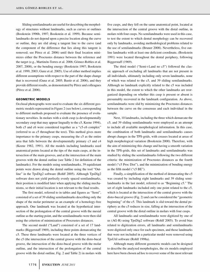
Table 4. Original and cross-validated percentages of correct classification for the five hominin species included in the CVA and for the

pooled sample.

Correct Correct Correct Correct Correct CorrectAFA EREC HEI NEA SAP TOTAL

OriginalSemi 87.5% 54.5% 70.8% 50.0% 77.5% 69.3%Land 75.0% 90.9% 66.7% 72.2% 80.0% 76.2%Semi+Land no c5 100.0% 100.0% 79.2% 72.2% 85.0% 84.1%c5 Proc Dist 87.5% 81.8% 62.5% 66.7% 77.5% 73.3%c5 BE 75.0% 63.6% 54.2% 72.2% 72.5% 67.3%Beginning c5 100.0% 100.0% 83.3% 77.8% 77.5% 83.2%

Cross-validatedSemi 62.5% 18.2% 62.5% 44.4% 75.0% 59.4%Land 62.5% 72.7% 58.3% 66.7% 75.0% 68.3%Semi+Land no c5 100.0% 81.8% 75.0% 61.1% 80.0% 72.2%c5 Proc Dist 62.5% 72.7% 58.3% 66.7% 75.0% 68.3%c5 BE 50.0% 63.6% 54.2% 66.7% 72.5% 64.4%Beginning c5 100.0% 81.8% 79.2% 72.2% 72.5% 77.2%

AFA=A. afarensis; EREC=H. erectus; HEI=H. heidelbergensis; NEA=H. neanderthalensis; SAP=H. sapiens.

morphometric methods is to include as much morphological in-

formation as possible from a given structure (Zelditch et al. 2004).

Particularly in evolutionary and developmental studies, novelties

tend to be key features distinguishing different taxa or distinguish-

ing different stages along an ontogenetic trajectory, and exclud-

ing novel features from datasets underestimates morphological

differences between clearly diverse groups, making it difficult to

discriminate them (Marcus et al. 2000).

Figure 8. Neighbor-joining trees based on the matrices of Procrustes distances between the mean shapes of the five best represented

hominin species (P. troglodytes has been used as outgroup). Note that branch lengths do not represent temporal spans, but Procrustes

distances.



Table 5. Procrustes distances measured between (1) H. heidel-

bergensis and H. neanderthalensis (HEI-NEA); (2) H. heidelbergen-

sis and H. sapiens (HEI-SAP); and (3) H. neanderthalensis and H.

sapiens (NEA-SAP), when using the six different models.

Procrustes distancesModel

HEI-NEA HEI-SAP NEA-SAP

Semi 0.0107 0.0206∗∗ 0.0210∗∗

Land 0.0850∗∗ 0.1481∗∗ 0.1959∗∗

Semi+Land no c5 0.0226∗ 0.0388∗∗ 0.0341∗∗

C5 Proc Dist 0.0483∗∗ 0.0860∗∗ 0.1100∗∗

C5 BE 0.0751∗∗ 0.1166∗∗ 0.1629∗∗

Beginning c5 0.0286∗ 0.0682∗∗ 0.0789∗∗

Mean LP3, LP4,LM1, UP3, UP4,UM11

0.0247 0.0385 0.0339

Significant differences in mean shapes based on 1000 random permutations

(P < 0.05). Two asterisks indicate highly significant differences (P < 0.01).1Mean values of the distances between the mean shapes of the three species

for lower first premolars (LP3), lower second premolars (LP4), lower first

molars (LM1), upper first premolars (UP3), upper second premolars (UP4),

and upper first molars (UM1).

It is worth noting the disparate amount of variance that each

model is able to recover, and the different distributions of that

variance among the different PCs, as observed in the scree plots

(Wagner 1984; Bruner 2009). The magnitude of the variance de-

pends on the number of landmarks included, and for this reason

the absolute value of the Procrustes variance is not directly com-

parable among the different models. Nonetheless, the differences

between the expected variance given a number of landmarks and

the actual variance measured when using each model point to dif-

ferences in the statistical properties of the models and to the fact

that the total variance is a mixture of effects of real variance and

number of landmarks. For example, lower variance is associated

with the dental outline described by semilandmarks, as indicated

by the low variance measured in the model “Semi,” whereas

the highest variance is associated with landmarks. Intermediate

approaches using both landmark and outline information are as-

sociated with intermediate variances that increase as information

related to the fifth cusp is added.

The existence of a leading eigenvector (associated with a

high eigenvalue) explaining a large proportion of the total variance

(large EV) has been proposed as a signal of morphological integra-

tion that can be found in covariance matrices extracted from cra-

nial and skeletal measurements of mammals; more uniform distri-

butions with intermediate eigenvalues correspond to less tightly

integrated structures (Wagner 1984; Young 2006; Pavlicev et al.

2009). In the present study, the distinct patterns of eigenvalue dis-

tributions in the models did not recover differences in the degree

of second molar morphological integration (all the models are

used to study the same morphology in the same sample). Rather,

they point to differences in the ability of the different configura-

tions of landmarks and semilandmarks to represent morphological

states. Previous geometric morphometric analyses of the hominin

dentition (Martinon-Torres et al. 2006; Gomez-Robles et al. 2007,

2008; Skinner et al. 2008) have shown that smooth variation of the

eigenvalue distribution, without clearly leading eigenvalues, is a

common pattern once the effect of size is removed by Procrustes

superimposition (Wagner 1984), and if main cusps are not gained

or lost in the analyzed sample. In any case, this discrepancy in

eigenvalue distribution must be taken into account when drawing

conclusions about morphological integration, because the choice

of determinate landmarks impacts the results in such a strong way.

By using the method proposed by Klingenberg (2008a), the

landmarks demarcating the c5 collapse to a null position in

the specimens lacking this cusp. One limitation of this method

is the increased weight—three times in this case—of the closest

null topological point when the cusp is absent. This fact biases the

Procrustes superimposition toward that point and multiplies the

variance with which that point contributes to the dataset. When

only a few landmarks are present, this multiplied contribution may

account for a large percentage of the total variance of the shape,

even if the variance is equally distributed among landmarks. This

same phenomenon will occur when semilandmarks are included

as there will be more variance associated with the outline, there-

fore driving the Procrustes superimposition and ordination.

The 2B-PLS and the values of the correlations of the two first

PCs in the six models show the clear correspondence between all

the models including the c5. This is not necessarily evidence of

the best performance among these models, rather it may be a con-

sequence of all the models recovering the same morphological

change, regardless of different landmark configurations. Due to

the relatively large sample size of H. sapiens and the morpho-

logical change associated with the loss of the fifth cusp (which

can be present or absent in H. sapiens molars), the first PC of

all the models including the c5 recovers intraspecific variation in

H. sapiens to a strong degree, rather than interspecific differences

in molar shape. This finding could indicate that these models are

unsuitable for taxonomic or phylogenetic studies when intraspe-

cific variation is found in the novelty, but it could also indicate that

these models are appropriate when that novelty is a characteristic

of a group of species.

PCA plots corresponding to each method show that the most

notable difference between the models is the clear separation of

four- and five-cusped molars in the four models including the

c5, and the absence of this separation in the remaining two mod-

els. As the morphospace representation recovering the most im-

portant morphological variations (Bruner 2009), the PCA plots

corresponding to both models that do not include the c5 fail

to show this separation. However, some groupings of molars



corresponding to individual species can be identified, highlight-

ing that interspecific differences are also located at the dental pe-

riphery (Martinon-Torres et al. 2006; Gomez-Robles et al. 2007,

2008) and at the landmarks that are not related to the c5. The

model “Semi+Land no c5” (including only landmarks that are

present in all the individuals) also recovers the presence or ab-

sence of the fifth cusp through the reorganization of the other

landmarks, although the exclusion of landmarks related to the c5

results in continuous variation (see also Skinner and Gunz 2010).

This continuous change is partially explained (nearly 10%) by

the total size of the molars, or, in other words, by evolutionary

allometric change, and approximately 13% of the variation is

explained by the relative and absolute size of c5. The morpholo-

gies corresponding to the extremes of these values are similar in

all three cases (Fig. 7). Larger molars and those with larger c5s

are also related to larger talonid basins (the occlusal depression

formed by the hypoconid or c3, entoconid or c4, and hypoconulid

or c5) and a characteristic dryopithecine (Y) pattern (Wood and

Abbott 1983; Bermudez de Castro and Nicolas 1995), whereas

smaller molars and those with small or absent c5s correspond to

smaller proportions of the talonid basin in comparison with the

trigonid basin and to the presence of cruciform (+) and X-shaped

patterns with respect to the arrangement of the four main cusps

(Bailey 2002; Irish and Guatelli-Steinberg 2003; Martinon-Torres

2006).

SUITABILITY OF THE MODELS

The models analyzed here show disparate results, although the

studied morphology is the same in all the cases (but see Navarro

et al. 2004 for a similar comparison of morphometric descriptors

that yields roughly similar results). It is important to note that

the analysis of 2D occlusal morphology of molars is suitable for

testing the landmark-based approach proposed by Klingenberg

(2008a). Nonetheless, this is not the most appropriate framework

for testing the performance of homology-free methods, because,

in this study, this approach is necessarily based on the analysis of

the 2D morphology of the dental periphery, rather than on the 3D

morphology of the occlusal surface.

The homology-free approach based on semilandmarks

(“Semi”) does not accurately recover morphological change in

the molars, as evinced by its low correlation with all the other

models, by the low percentages of correct assignment and wrong

inference of hominin phylogeny, by the unclear separation of

four- and five-cusped molars, and by the clear underestimation of

Procrustes distances (Table 5). This is not surprising, because this

model is based only on the analysis of the peripheral molar shape,

and the most important morphological changes are determined

by the occlusal features (e.g., the location of cusp tips and the

intersection of the main grooves; Wood and Abbott 1983). Other

homology-free methods, such as eigenshape analysis or Fourier

analysis, could be more sensitive to recovering the peripheral

morphology, but by using semilandmarks, landmark-based and

homology-free approaches can be combined (Adams et al. 2004;

Monteiro et al. 2004), facilitating a comparison of results from

both types of analyses and combined approaches. Nonetheless, it

is important to note that the analysis of 3D surfaces, in which the

information regarding to the topography of the analyzed structure

in the “z” axis is included, would provide stronger results and a

more intuitive visual output (Polly and MacLeod 2008).

Regarding the landmark-based approach including land-

marks demarcating the evolutionary novelty (model “Land”),

it overcomes the methodological problems associated with

homology-free approaches (Bookstein et al. 1982; Erlich et al.

1983; Zelditch et al. 1995). Nonetheless, although in this partic-

ular example the location of the landmarks demarcating the c5

is easy to infer in four-cusped molars, as it is situated between

the third and fourth cusps, these landmarks are not necessar-

ily homologous in an anatomical sense. Additionally, this model

needs to include some landmarks located at the molar periphery as

reference points. The anatomical homology of these outline land-

marks is also debatable (O’Higgins 2000), and their unavoidable

deficient definition highly increases Procrustes variance in this

model. However, only a few landmarks are available in hominin

teeth (Biggerstaff 1969; Gomez-Robles et al. 2008), and the mor-

phology of the different species cannot be correctly discriminated

if the information regarding the outline is not included, either by

using a complete set of semilandmarks or some peripheral points.

Perhaps surprisingly, the model “Semi+Land no c5,” which

represents the classic method that avoids explicitly addressing

novelties, provides a high percentage of correct classification

and gives rise to a phylogeny that best reflects hominin phylo-

genetic relationships. This model, however, does not recover the

expected morphological distances between H. heidelbergensis, H.

neanderthalensis, and H. sapiens (HEI-NEA<HEI-SAP<NEA-

SAP). Rather, it evinces a different pattern of distances (HEI-

NEA<NEA-SAP<HEI-SAP) that gives rise nevertheless to the

most correct phylogeny once polarity is taken into account by

using an outgroup. Furthermore, when the c5 is not explicitly in-

cluded in the dataset, the presence or absence of this cusp cannot

be unequivocally discriminated in the PCA plots or in the TPS-

grids. Instead, an area of the morphospace where both four- and

five-cusped molars overlap in their ranges of variation is identi-

fied, and the corresponding grids are not completely clear at indi-

cating the cusp number (Skinner and Gunz 2010). Additionally,

Procrustes distances among individuals are underestimated when

using this model in comparison with teeth that do not include any

evolutionary novelties (Table 5), the morphological differences in

these cases are expected to be smaller (Adams et al. 2004).

Both models including landmarks demarcating the c5 and

sliding semilandmarks (“c5 Proc Dist” and “c5 BE”) show



different results, although they are based on exactly the same

set of landmarks and semilandmarks. The two different methods

to slide semilandmarks recover different aspects of morphological

changes; the former minimizes variation of the affine and non-

affine part of the morphological transformation and is especially

interesting in systematic approaches to morphological variation

(Gunz et al. 2005; Bastir et al. 2006), and the later minimizes the

nonaffine part of the shape variation and is suitable when features

of the spline are interpreted as morphological information (Book-

stein 1991, 1997; Gunz et al. 2005; Bastir et al. 2006). The only

model using the minimization of bending energy as the sliding

criterion provides percentages of correct classification even lower

than those attained using only semilandmarks (Table 4, original

percentages), although the PCs on which the assignment test is

based account for a higher percentage of variance in this model

than in any other model. Additionally, the creases in the TPS-grids

corresponding to these models are caused by the fact that several

outline points get collapsed to a single position and “trap” the grid

when the c5 is absent.

Finally, the model “Beginning c5,” which includes only one

landmark related to the c5 (the location of which is related to the

size of this cusp) allows for easily and directly discerning the pres-

ence or absence of novelties by grouping together individuals with

or without that substructure in the PCA. Furthermore, this model

results in one of the highest percentages of correct classification

and has the benefit of avoiding underestimation of the Procrustes

distances, as has been described for the model excluding the c5.

Nonetheless, this model is not able to accurately reflect phylo-

genetic relationships among hominin species, partially due to the

fact that H. sapiens and H. heidelbergensis are clustered together

because they are the only species in this sample with four-cusped

molars (or, in other words, with a mean shape where the strong re-

duction of the fifth cusp is apparent). Mathematically, this model

circumvent the triple-weighting of the information relative to the

c5 and a subsequent inflation of the variance described for the

models demarcating the fifth cusp, although the morphological

information relative to the analyzed evolutionary novelty is still in-

cluded. Again, the criterion of anatomical homology is not strictly

fulfilled, rather it is relaxed in favor of a more functional approach.

The results of this work compel us to question the extent

to which these results can be extrapolated to other contexts, as

the inclusion of novel features in morphological analyses of other

skeletal parts and other organisms, in studies of ontogeny, and in

3D approaches to the study of morphology. Although the use of

similar approaches based on one or more key landmarks recov-

ering the presence or absence of the novel feature can be useful,

the choice of landmarks should be justified and based on knowl-

edge of the structure studied (Oxnard and O’Higgins 2009), and

the impact of this choice on the subsequent analyses should be

measured and considered in light of the results.

ConclusionsThis research has aimed to test, using a practical example, differ-

ent methods to include evolutionary novelties in geometric mor-

phometric studies. The problem of (sub)structures gained or lost

during evolution has been traditionally ignored in geometric mor-

phometric analyses by excluding these features. However, some

recent studies have addressed this problem, proposing methods to

explicitly include these traits. A comparison of six such methods

that employ some of the most commonly used sampling strategies

demonstrate clear differences in the morphological changes recov-

ered when using different approaches to analyze novel features.

When analyzing hominin lower second molar morphology in an

evolutionary framework, an approach combining semilandmarks,

landmarks common to all specimens, and only one landmark re-

lated to the novel structure provides reasonably accurate results

(in terms of taxonomic assignment and phylogenetic reconstruc-

tion). This method also allows easy discernment of the presence

or absence of evolutionary novelties, and circumvents mathemat-

ical problems resulting from the demarcation of the novel trait,

a method recently proposed by some authors. In any case, the

criterion of anatomical homology must be relaxed if novel struc-

tures are to be included in geometric morphometric studies, ei-

ther by using homology-free approaches or by using landmarks

that do not have an explicit anatomical correspondence between

specimens.

ACKNOWLEDGMENTSWe are especially grateful to the organizers of the First Iberian Symposiumon Geometric Morphometrics for the opportunity of discussing someaspects of this work. Special thanks are also due to E. Bruner for constantdiscussion and ideas to improve this study. We are deeply grateful toP. D. Polly for his thorough revision of the manuscript and for makingus think about the problem of novelties, and to M. Lawing for sharingwith us her ideas. Thanks to A. Muela for photographing part of thesample, and to D. Sanchez-Martın for his technical support. This workwas supported by funding from the Direccion General de Investigacionof the Spanish MICINN (Project No. CGL2009-12703-C03-01), Junta deCastilla y Leon (Project No. GR-249). LP-S. have the benefit of FundacionAtapuerca research grant.

LITERATURE CITEDAdams, D. C., F. J. Rohlf, and D. Slice. 2004. Geometric morphometrics:

ten years of progress following the ‘Revolution’. Ital. J. Zool. 71:5–16.

Arsuaga, J. L., I. Martınez, A. Gracia, and C. Lorenzo. 1997. The Sima delos Huesos crania (Sierra de Atapuerca, Spain). A comparative study.J. Hum. Evol. 33:219–281.

Bailey, S. E. 2002. Neanderthal dental morphology: implications for modernhuman origins. Ph.D. dissertation. Arizona State University.

Bailey, S. E., and J. M. Lynch. 2005. Diagnostic differences in mandibularP4 shape between Neandertals and anatomically modern humans. Am.J. Phys. Anthropol. 126:268–277.

Bastir, M., A. Rosas, and P. O’Higgins. 2006. Craniofacial levels and themorphological maturation of the human skull. J. Anat. 209:637–654.



Bermudez de Castro, J. M., and M. E. Nicolas. 1995. Posterior dental sizereduction in hominids: the Atapuerca evidence. Am. J. Phys. Anthropol.96:335–356.

Biggerstaff, R. H. 1969. The basal area of posterior tooth crown components:the assessment of within tooth variation of premolars and molars. Am.J. Phys. Anthropol. 31:163–170.

Blackith, R. E., and R. A. Reyment. 1971. Multivariate morphometrics. Aca-demic Press, London.

Bookstein, F. L. 1989. Principal warps: thin-plate splines and the decomposi-tion of deformations. IEEE T. Pattern Anal. 11:567–585.

———. 1991. Morphometric tools for landmark data. Cambridge Univ. Press,Cambridge.

———. 1996a. Combining the tools of geometric morphometrics. Pp. 131–151 in L. F. Marcus, M. Corti, A. Loy, G. J. P. Naylor, and D. Slice, eds.Advances in morphometrics. Plenum Press, New York.

———. 1996b. Applying landmark methods to biological outline data.Pp. 79–87 in K. V. Mardia, C. A. Gill, and I. L. Dryden, eds. Imagefusion and shape variability techniques. Leeds Univ. Press, Leeds.

———. 1997. Landmark methods for forms without landmarks: morphomet-rics of group differences in outline shape. Med. Image Anal. 1:225–243.

———. 2000. Creases as local features of deformation grids. Med. ImageAnal. 4:93–110.

Bookstein, F. L., R. E. Strauss, J. M. Humphries, B. Chernoff, R. L. Elder,and G. R. Smith. 1982. A comment upon the uses of Fourier methods insystematics. Syst. Zool. 31:85–92.

Bookstein, F., K. Schafer, H. Prossinger, H. Seidler, M. Fieder, C. Stringer,G. W. Weber, J. L. Arsuaga, D. E. Slice, F. J. Rohlf, et al. 1999. Compar-ing frontal cranial profiles in archaic and modern Homo by morphometricanalysis. Anat. Rec. (New Anat.) 257:217–224.

Bookstein, F. L., P. Gunz, P. Mitteroecker, H. Prossinger, K. Schaefer, and H.Seidler. 2003. Cranial integration in Homo: singular warps analysis ofthe midsagittal plane in ontogeny and evolution. J. Hum. Evol. 44:167–187.

Bruner, E. 2008. Comparing endocranial form and shape differences in modernHumans and Neandertals: a geometric approach. PaleoAnthropology2008:93–106.

———. 2009. The structure of the morphospace as a representation of abiological model. Paleontologia y Evolucio Memoria especial n◦ 3:3.

Cardini, A., and S. Elton. 2008. Does the skull carry a phylogenetic signal?Evolution and modularity in the guenons. Biol. J. Linn. Soc. 93:813–834.

Erlich, R., R. B. Pharr, and N. Healy-Williams. 1983. Comments on thevalidity of Fourier descriptors in systematics: a reply to Bookstein et al.Syst. Zool. 32:202–206.

Escoufier, Y. 1973. Le traitement des variables vectorielles. Biometrics29:751–760.

Felsenstein, J. 2005. PHYLIP (Phylogeny Inference Package) version 3.6.Distributed by the author. Department of Genome Sciences, Univ. ofWashington, Seattle.

Frieß, M. 2003. An application of the relative warps analysis to problemsin human paleontology—with notes on raw data quality. Image Anal.Stereol. 22:63–72.

Frieß, M., and M. Baylac. 2003. Exploring artificial cranial deformation usingelliptic Fourier analysis of Procrustes aligned outlines. Am. J. Phys.Anthropol. 122:11–22.

Gomez-Robles, A. 2010. Analisis de la forma dental en la filogenia humana.Tendencias y modelos evolutivos basados en metodos de morfometrıageometrica. Ph.D. dissertation. Universidad de Granada.

Gomez-Robles, A., M. Martinon-Torres, J. M. Bermudez de Castro, A.Margvelashvili, M. Bastir, J. L. Arsuaga, A. Perez-Perez, F. Estebaranz,and L. M. Martınez. 2007. A geometric morphometric analysis of ho-minin upper first molar shape. J. Hum. Evol. 53:272–285.

Gomez-Robles, A., M. Martinon-Torres, J. M. Bermudez de Castro, L. Prado,S. Sarmiento, and J. L. Arsuaga. 2008. Geometric morphometric analysisof the crown morphology of the lower first premolar of hominins, withspecial attention to Pleistocene Homo. J. Hum. Evol. 55:627–638.

Gunz, P., P. Mitteroecker, and F. Bookstein. 2005. Semilandmarks in three di-mensions. Pp. 73–98 in D. Slice, ed. Modern morphometrics in physicalanthropology. Kluwer Academic, Dodretch.

Harvati, K., J.-J. Hublin, and P. Gunz. 2010. Evolution of middle-late Pleis-tocene human cranio-facial form: a 3-D approach. J. Hum. Evol. 59:445–464.

Irish, J. D., and D. Guatelli-Steinberg. 2003. Ancient teeth and modern humanorigins: an expanded comparison of African Plio-Pleistocene and recentworld dental samples. J. Hum. Evol. 45:113–144.

Jernvall, J. 2000. Linking development with generation of novelty in mam-malian teeth. Proc. Natl. Acad. Sci. USA 97:2641–2645.

Jernvall, J., and H.-S. Jung. 2000. Genotype, Phenotype, and developmentalbiology of molar tooth characters. Yrbk. Phys. Anthropol. 43:171–190.

Jernvall, J., P. Kettunen, I. Karavanova, L. B. Martin, and I. Thesleff. 1994.Evidence for the role of the enamel knot as a control center in mammaliantooth cusp formation: non-dividing cells express growth stimulating Fgf-4 gene. Int. J. Dev. Biol. 38:463–469.

Keene, H. J. 1982. The morphogentic triangle: a new conceptual tool for ap-plication to problems in dental morphogenesis. Am. J. Phys. Anthropol.59:281–287.

———. 1991. On heterochrony in heterodonty: a review of some problemsin tooth morphogenesis and evolution Yrbk. Phys. Anthropol. 34:251–282.

———. 1994. On the classification of C6 (tuberculum sextum) of themandibular molars. Hum. Evol. 9:231–247.

Keranen, S. V. E., T. Aberg, P. Kettunen, I. Thesleff, and J. Jernvall. 1998.Association of developmental regulatory genes with the development ofdifferent molar tooth shapes in two species of rodents. Dev. Genes Evol.208:477–486.

Klingenberg, C. P. 2008a. Novelty and “homology-free” morphometrics:what’s in a name? Evol. Biol. 35:186–190.

———. 2008b. MorphoJ. Faculty of Life Sciences, Univ. of Manchester,Manchester, UK.

———. 2009. Morphometric integration and modularity in configurations oflandmarks: tools for evaluating a priori hypotheses. Evol. Dev. 11:405–421.

Klingenberg, C. P., and N. A. Gidaszewski. 2010. Testing and quantifyingphylogenetic signals and homoplasy in morphometric data. Syst. Biol.59:245–261.

Lockwood, C. A., W. H. Kimbel, and J. M. Lynch. 2004. Morphometricsand hominoid phylogeny: support for a chimpanzee-human clade anddifferentiation among great ape subspecies. Proc. Natl. Acad. Sci. USA101:4356–4360.

Lohmann, G. 1983. Eigenshape analysis of microfossils: a general morpho-metric procedure for describing changes in shape. Math. Geol. 15:659–672.

Love, A. C. 2003. Evolutionary morphology, innovation, and the synthesis ofevolutionary and developmental biology. Biol. Philos. 18:309–345.

MacLeod, N. 1999. Generalizing and extending the eigenshape method ofshape space visualization and analysis. Paleobiology 25:107–138.

———. 2001. Landmarks, localization, and the use of morphometrics inphylogenetic analysis. Pp. 197–233 in G. Edgecombe, J. Adrain, and B.Lieberman, eds. Fossils, phylogeny, and form: an analytical approach.Kluwer Academic Plenum, New York.

Marcus, L. E., E. Hingst-Zaher, and H. Zaher. 2000. Application of landmarkmorphometrics to skulls representing the orders of living Mammals.Hystrix 11:27–47.



Martinon-Torres, M. 2006. Evolucion del aparato dental en homınidos: estu-dio de los dientes humanos del Pleistoceno de la Sierra de Atapuerca(Burgos). Ph.D. dissertation. Universidad de Santiago de Compostela.

Martinon-Torres, M., M. Bastir, J. M. Bermudez de Castro, A. Gomez, S.Sarmiento, A. Muela, and J. L. Arsuaga. 2006. Hominin lower sec-ond premolar morphology: evolutionary inferences through geometricmorphometric analysis. J. Hum. Evol. 50:523–533.

Mitteroecker, P., and P. Gunz. 2009. Advances in geometric morphometrics.Evol. Biol. 36:235–247.

Monteiro, L. R., L. Guillermo, L. Rivera, and A. P. M. Beneditto. 2004.Geometric methods combining contour and landmark information in thestatistical analysis of biological shape. Pp. 336–355 in R. Mondaini, ed.Third Brazilian symposium on mathematical and computational biology.E-papers, Rio de Janeiro.

Muller, G. B., and G. P. Wagner. 1991. Novelty in evolution: restructuring theconcept. Annu. Rev. Ecol. Syst. 22:229–256.

Muller, G. B., and S. A. Newman. 2005. The innovation triad: an EvoDevoagenda. J. Exp. Zool. 304B:487–503.

Navarro, N., X. Zatarain, and S. Montuire. 2004. Effects of morphometricdescriptor changes on statistical classification and morphospaces. Biol.J. Linnean Soc. 83:243–260.

O’Higgins, P. 2000. The study of morphological variation in the hominid fossilrecord: biology, landmarks and geometry. J. Anat. 197:103–120.

Oxnard, C., and P. O’Higgins. 2009. Biology clearly needs morphometrics.Does morphometrics need biology? Biol. Theor. 4:84–97.

Pavlicev, M., J. Cheverud, and G. Wagner. 2009. Measuring morphologicalintegration using eigenvalue variance. Evol. Biol. 36:157–170.

Perez, S. I., V. Bernal, and P. N. Gonzalez. 2006. Differences between slidingsemi-landmark methods in geometric morphometrics, with an applica-tion to human craniofacial and dental variation. J. Anat. 208:769–784.

Pigliucci, M. 2008. What, if anything, is an evolutionary novelty? Philos. Sci.75:887–898.

Polly, P. D. 2001. On morphological clocks and paleophylogeography: towardsa timescale for Sorex hybrid zones. Genetica 112–113:339–357.

———. 2003. Paleophylogeography of Sorex araneus (Insectivora, Sorici-dae): molar shape as a morphological marker for fossil shrews. Mam-malia 67:233–244.

———. 2008a. Developmental dynamics and G-matrices: can morphometricspaces be used to model phenotypic evolution? Evol. Biol. 35:83–96.

———. 2008b. Adaptive zones and the Pinniped ankle: a three-dimensionalquantitative analysis of carnivoran tarsal evolution. Pp. 167–196 in E.Sargis and M. Dagosto, eds. Mammalian evolutionary morphology, atribute to Frederick S. Szalay. Springer, Dordretch.

Polly, P. D., and N. MacLeod. 2008. Locomotion in fossil Carnivora: anapplication of eigensurface analysis for morphometric comparison of3D surfaces. Paleontologia Electronica 11:13p. Available at http://palaeontologia-electronica.earthsci.carleton.ca/2008 2/135/135.pdf.

Rohlf, F. J. 1998a. TpsUtil. TpsSeries. Department of Ecology and Evolution,SUNY, Stony Brook, New York.

———. 1998b. TpsRelw. TpsSeries. Department of Ecology and Evolution,SUNY, Stony Brook, New York.

———. 1998c. TpsRegr. TpsSeries. Department of Ecology and Evolution,SUNY, Stony Brook, New York.

———. 2005. TpsDig2. TpsSeries. Department of Ecology and Evolution,SUNY, Stony Brook, New York.

Rohlf, F. J., and D. Slice. 1990. Extension of the Procrustes method for theoptimal superimposition of landmarks. Syst. Zool. 39:40–59.

Rohlf, F. J., and L. E. Marcus. 1993. A revolution in morphometrics. TrendsEcol. Evol. 8:129–132.

Rohlf, F. J., and M. Corti. 2000. Use of two-block partial least-squares tostudy covariation in shape. Syst. Biol. 49:740–753.

Roth, V. L., and J. M. Mercer. 2000. Morphometrics in development andevolution. Am. Zool. 40:801–810.

Saitou, N., and M. Nei. 1987. The neighbor-joining method: a new methodfor reconstructing phylogenetic trees. Mol. Biol. Evol. 4:406–425.

Salazar-Ciudad, I. 2006. On the origins of morphological disparity and itsdiverse developmental bases. BioEssays 28:1112–1122.

Scott, G. R., and C. G. Turner. 1997. The Anthropology of modern humanteeth: dental morphology and its variation in recent human populations.Cambridge Univ. Press, Cambridge.

Sereno, P. C. 2007. Logical basis for morphological characters in phylogenet-ics. Cladistics 23:565–587.

Sheets, H. D. 2001. IMP (Integrated Morphometrics Package). Department ofPhysics, Canisius College, Buffalo.

Shen, L., H. Farid, and M. A. McPeek. 2009. Modeling three-dimensional mor-phological structures using spherical harmonics. Evolution 63:1003–1016.

Skinner, M. M., P. Gunz, B. A. Wood, and J.-J. Hublin. 2008. Enamel-dentinejunction (EDJ) morphology distinguishes the lower molars of Australo-pithecus africanus and Paranthropus robustus. J. Hum. Evol. 55:979–988.

———. 2009. How many landmarks? Assessing the classification accuracyof Pan lower molars using a geometric morphometric analysis of theocclusal basin as seen at the enamel-dentine junction. Front. Oral Biol.13:23–29.

Skinner, M. M., and P. Gunz. 2010. The presence of accessory cusps inchimpanzee lower molars is consistent with a patterning cascade modelof development. J. Anat. 217:245–253.

Turner, C. G., C. R. Nichol, and G. R. Scott. 1991. Scoring procedures forkey morphological traits of the permanent dentition: the Arizona StateUniversity Dental Anthropology System. Pp. 13–31 in M. Kelley and C.Larsen, eds. Advances in dental anthropology. Wiley Liss, New York.

Wagner, G. P. 1984. On the eigenvalue distribution of genetic and pheno-typic dispersion matrices: evidence for a nonrandom organization ofquantitative character variation. J. Math. Biol. 21:77–95.

Wood, A. R., M. L. Zelditch, A. N. Rountrey, T. P. Eiting, H. D. Sheets,and P. D. Gingerich. 2007. Multivariate stasis in the dental morphologyof the Paleocene-Eocene condylarth Ectocion. Paleobiology 33:248–260.

Wood, B. A., and S. A. Abbott. 1983. Analysis of the dental morphology ofPlio-Pleistocene hominids I. Mandibular molars: crown area measure-ments and morphological traits. J. Anat. 136:197–219.

Wood, B. A., and C. A. Engleman. 1988. Analysis of the dental morphology ofPlio-Pleistocene hominids: V. Maxillary postcanine tooth morphology.J. Anat. 161:1–35.

Xing, S., M. Zhou, and W. Liu. 2009. Crown morphology and variation ofthe lower premolars of Zhoukoudian Homo erectus. Chinese Sci. Bull.54:3905–3915.

Young, N. M. 2006. Function, ontogeny and canalization of shape variance inthe primate scapula. J. Anat. 209:623–636.

Zelditch, M. L., W. L. Fink, and D. L. Swiderski. 1995. Morphometrics,homology, and phylogenetics: quantified characters as synapomorphies.Syst. Biol. 44:179–189.

Zelditch, M. L., D. L. Swiderski, H. D. Sheets, and W. L. Fink. 2004. Geo-metric morphometrics for biologists: a primer. Elsevier Academic Press,San Diego, CA.

Associate Editor: G. Hunt


evolutionary novelties and losses in geometric

Documents