Evolution of International Stock and Bond Market Integration: Influence

of the European Monetary Union

Suk-Joong Kim Fari Moshirian1

Eliza Wu

School of Banking and Finance, University of New South Wales, Sydney, NSW 2052, Australia.

Abstract

This paper examines the dynamic relationship between daily stock and government bond returns of selected countries over the past decade to infer the state and progress of inter-financial market integration. We proceed to empirically investigate the influence of the European Monetary Union (EMU) on time-variations in inter-stock-bond market integration/segmentation dynamics using a two-step procedure. First, we document the downward trends in time-varying conditional correlations between stock and bond market returns in European countries, Japan and the US. Second, we investigate the causality and determinants of this interdependent relationship, in particular, whether the various macroeconomic convergence criteria associated with the EMU have played a significant role. We find that real economic integration and the reduction in currency risk have generally had the desired effect on financial integration but monetary policy integration may have created uncertain investor sentiments on the economic future of the European monetary union, thereby stimulating a flight to quality phenomenon. JEL Classification: C32; E44; F3; G14; G15 Keywords: Euro, volatility, currency unions, stock-bond correlations, time-varying financial market integration, flight to quality, optimal currency area.

Final Draft: February 2005

1 Corresponding author; email: f.moshirian@unsw.edu.au. We thank an anonymous reviewer and seminar participants in the School of Banking and Finance at UNSW for providing helpful comments on earlier drafts. All errors remain our own.

1

1. Introduction

Financial market integration is a central theme in International Finance and the

benefits of economic growth via risk sharing, improvements in allocational efficiency and

reductions in macroeconomic volatility and transaction costs are all well accepted (see Prasad

et al., 2003 and Baele et al., 2004). Whilst financial market integration encompasses many

different aspects of the complex inter-relationships across various financial markets, we focus

on the nature and extent of interdependence (co-movements) across daily asset returns. 2

Whilst international integration within specific financial asset markets has received much

attention, the subject of integration across different financial asset markets has not, despite its

importance for investors’ asset allocation and portfolio risk management decisions. This study

investigates stock and bond market integration over time within a common market jurisdiction

as we are motivated by: recent developments on stock-bond return co-movements in financial

economics; and the historical European Economic and Monetary union (EMU) experience.

Co-movements in asset market returns provide indirect evidence on financial markets’

expectations and their reaction to common information that are priced into different asset

types. To our best knowledge, co-movements in stock and bond returns have not been

previously interpreted in an inter-financial market integration context and to this end, our

main contribution is in merging these two strands of literature to shed new light on both.

Moreover, with the implementation of a currency union and associated stabilization of

macroeconomic fundamentals in Europe, we also ask whether there have been any influences

on the integration process between stock and bond markets as this has not been addressed in

the existing market integration literature.

2 Studies sharing this focus include Bekaert and Harvey (1995), Bracker et al. (1999), Karolyi and Stulz (1996)

and Longin and Solnik (1995).

2

The nature of stock-bond market co-movements has perplexed researchers in financial

economics for years and there have been many attempts to understand their fundamental

relationship. Existing stock-bond studies are generally in agreement on how stock and bond

returns co-move over time but not why they co-move. Early studies to address the latter can

be represented by Campbell and Ammer (1993) as they implicitly assume time-invariance in

the stock-bond relation, and conclude that observed levels cannot be justified by economic

fundamentals. In this thread, Engsted and Tangguard (2001) is relevant for the European

markets. Most recently, researchers modeled the time-varying risk premia in their

investigation and established that stock and government bond returns exhibit a modest

positive correlation over a long horizon but the relationship is a dynamic one, meaning that

the amount of portfolio diversification with a given asset allocation is constantly changing

(see inter alia Connolly et al., 2005 and Fleming et al., 2003). In particular, Cappiello et al.

(2003) and Scruggs and Glabadanidis (2003) investigate the asymmetric nature of stock and

bond market conditional variances and their comovement. In the asset pricing vein, Ilmanen

(1995) and Barr and Priestley (2004) suggest that world stock and bond markets are largely

segmented and that further understanding of their joint behaviour is needed.

Informational linkages have formed the basis of most recent theoretical models on

time-varying stock-bond return co-movements. There are two main channels through which

information drives that relationship: 1) Common sources of information influencing

expectations in both stock and bond markets at the same time and 2) Sources of information

that only alter expectations in one market but spill over into the other market. Informational

spillovers between the two markets are the crux of dynamic cross-market hedging studies (see

Fleming et al., 1998 and Kodres and Pritsker, 2002) and the motivation behind analyzing co-

movements in stock and bond market liquidities and the interaction with returns, volatility and

order flow in Chordia et al. (2005). It is argued that a shock in one asset market may generate

3

cross-market asset rebalancing thereby generating volatility linkages. Generally, government

bonds are deemed to be a safe haven for investors engaging in a “flight to quality” in times of

financial turmoil. As investors substitute safe assets for their risky ones, bond and stock

market returns become negatively correlated (see Chordia et al., 2005, Connolly et al., 2005

and Hartmann et al., 2004). Most recently, stock market uncertainty has been provided by

Connolly et al. (2005) as a key explanation for the stock-bond return relation. They use

implied volatilities from equity index options to reflect stock market uncertainty, emphasizing

that this should be positively related to economic-state uncertainty in the sense of Veronesi

(1999). In spite of existing work, the explanation for long-term co-movements in stock and

bond returns remains conjectural.

In this paper, we contribute to the literature by interpreting stock-bond return co-

movements in a new light. They have traditionally been modeled as statistical

contemporaneous correlations or covariances but have not been viewed as an integral aspect

of inter-stock-bond market integration. Hence, we analyse the extent to which international

stock-bond market integration has been influenced by the EMU by documenting and

determining the conditional correlation dynamics between daily stock and bond returns in a

bivariate EGARCH model from 2/3/1994 to 19/9/2003. Our main hypothesis is that economic

policies directed at achieving convergence in exchange rates, monetary stance and the real

economy (three channels which have characterized the degree of economic integration across

countries with the EMU) have been relevant and critical common influences on the extent of

systemic stock and bond market integration in Europe and the rest of the world. We utilize

additional information captured in a seemingly unrelated regression (SUR) to evaluate the

significance of these economic channels amongst seasonal effects.

Our new findings are i) as intra-stock and bond market integration with the EMU has

strengthened in the sample period, inter-stock-bond market integration has trended

4

downwards to zero and even negative mean levels in most European countries, Japan and the

US, consistent with a flight to quality phenomena in international financial markets; ii) cross-

market volatilities have overall stabilizing effects but bond market return shocks have more

influence; iii) the EMU has caused the inter-stock-bond market segmentation dynamics (in a

Granger sense) only in European countries; iv) real economic integration with the EMU and

reduction in currency risk with the introduction of the Euro have generally stimulated inter-

financial market integration but increasing monetary policy convergence with the EMU may

have created uncertain investor sentiments in the international financial system; and v) there

is no evidence of calendar effects in international inter-stock-bond market integration,

particularly the January and day of the week effect.

The remainder of this paper is organized as follows. Section 2 introduces the data used

for documenting and explaining the dynamics of stock-bond market integration. Section 3

focuses discussion on model selection whilst Section 4 considers the progress of financial

integration between stock and government bond markets over time. Section 5 investigates the

causality and determinants of time varying integration across stock and bond markets. Finally,

concluding remarks are made in Section 6.

2. Data description and statistics

Daily Bond and Stock market returns

Our empirical analysis is conducted for a sample set of countries that fall into two

distinct groups: 1) Euro zone members that have adopted the Euro as a common currency -

France, Germany, Italy, and Spain having the largest and most developed financial markets in

the EMU and 2) Non-Euro zone countries which comprise the UK, which has opted to stay

out of the EMU and Japan and US as they are the world’s other two major financial markets,

enabling inferences to be made on the EMU’s global impacts.

5

We employ the national total market return share indices from Datastream

International and total return government bond indices for maturities greater than 10 years

obtained from Bloomberg for the two groups of countries.3 Government bonds with more

than 10 years to maturity have been used to effectively match their duration with stocks,

which are generally viewed as long-term investments. The indices are all in local currency

units with daily frequency from 2 March 1994 to 19 September 2003, determined by the

availability of daily bond market indices for all countries in the sample. The continuously

compounded market returns examined in this study are measured as the natural logarithms of

the ratios of closing index levels from one trading day to the next such that,

( )1ln / 100it t tR P P−= × for market i on day t. Local (unhedged) currency returns are used in

this study to investigate the impact of changes in exchange rate risk induced by the

introduction of the Euro for domestic investors. Daily frequency is important as co-

movements in the stock and bond returns often change on a rapid basis as investors shift their

domestic asset allocation. Weekly stock and bond return data have been used by Cappiello et

al. (2003) to model cross-country stock-bond return correlations for a sample of European and

Australasian countries and the US.

To provide some perspective on the data, Table 1 reports the statistical properties of

the daily bond and stock market returns for each sample country and the (market

capitalization) value weighted average for the Euro zone. The pre- and post-Euro sub-sample

statistics are shown in panels A and B, respectively.4 Bonds have only outperformed stocks in

the post-Euro period but were less volatile in both periods. This is consistent with major

declines in world equity prices since the collapse of the technology boom in 2001. In the pre-

Euro sub-sample period, stock returns exceeded average bond returns for all countries except

3 Total return on bonds capture the coupon payments that are reinvested back into the bonds forming the index as well as bond price changes and similarly, total return indices on shares account for price changes and dividend reinvestments.

6

Italy and Japan. These observations are all consistent with well-documented stylized facts on

stock and bond returns (eg., see Connolly et al., 2005, Li, 2002 and Scruggs and

Glabadanidis, 2003). The distributions of these stock and bond market returns are statistically

non-normal, and the standardized return series are highly persistent and heteroskedastic on the

basis of univariate i.i.d. tests. The significance of the bivariate i.i.d. test statistics for each pair

of stock and bond index returns indicates that the first and second moments of these series

move closely together. Henceforth, modeling of these return series must address the bivariate

and fat-tailed nature of these distributions in addition to the high degree of univariate and

bivariate serial correlations.

Explanatory Variables

The list of variable definitions and data sources used in this study for the real and

monetary convergence and exchange rate stability criteria is shown in Appendix A. First,

correlations in nominal short term interest rates, inflation and real short term interest rates

proxy convergence in monetary policy, and second, the size of the trade sector, intra-regional

trade integration and correlations in output and term structure and dividend yield changes

proxy the degree of real economic integration. Our probe into the link between financial and

economic integration in the vein of Fratzscher (2002) and Kim et al.’s (in-press) European

stock market studies provide new insights on the potential determinants of stock and bond co-

movements. Lastly, we generate conditional exchange rate volatilities using univariate

GARCH(1,1) estimations for the change in local currency : Euro exchange rates to capture

past information in exchange rates. 5

4 Summary statistics are available for the full sample period upon request. 5 The European Currency Unit (ECU) was used prior to the Euro’s launch. As a robustness check, rolling

standard deviations over 3 month time windows were also used to proxy exchange rate volatility and there was

no qualitative improvement in our regression results.

7

Furthermore, we build on Connolly et al.’s (2005) study and use implied volatilities

from equity index options as a proxy for economic uncertainty in the international financial

system. We use the Chicago Board of Options Exchange (CBOE)’s volatility index (VIX) and

the German DAX equity index (VDAX) for explaining inter-stock-bond market integration in

the US and Japan and all the European countries respectively.

3. Econometric Model

This study aims to examine whether the establishment of the EMU has induced a

dynamic change in inter-stock-bond market integration by making inferences from the

behavior of their daily conditional volatility interdependencies and time-varying conditional

correlations. There is existing support for the notion that market integration influences the

conditional asset return generating process (see Bekaert and Harvey, 2003).

Whilst the use of conditional econometric models capable of capturing asymmetric

volatility has proliferated in stock market studies, government bond markets have not been

dealt with in the same way.6 As Scruggs and Glabadanidis (2003) strongly rejected symmetric

models of conditional second moments for stock and bond returns, we model the joint return

generating process of stock and bond markets with a bivariate exponential generalized

autoregressive conditional heteroskedasticity (EGARCH) model incorporating a bivariate

student’s t conditional density function for the innovation vector to explicitly account for

positive and negative shocks and fat tails in returns. Previous studies have found that the

logarithmic specification in Nelson’s (1991) EGARCH model with a suitable distributional

6 See Wu (2001) and references therein for a survey of asymmetric volatilities in stock market studies and tests

of the leverage and volatility feedback effects.

8

assumption fits financial data well.7 The advantage of employing the t-distribution is that the

unconditional leptokurtosis observed in most high-frequency asset price data sets can appear

as conditional leptokurtosis and still converge asymptotically to the Normal distribution as

1/D (D being the degrees of freedom) approaches zero (usually in lower-frequency data). This

provides added flexibility to our methodology.

A bivariate EGARCH-t model with time-varying conditional correlations is a

worthwhile methodological contribution to the existing stock-bond co-movement literature.

The use of regime switching models in Connolly et al. (2005) requires volatility states to be

probabilistically set and asymmetric dynamic conditional correlation models in Cappiello et

al. (2003) and Scruggs and Glabadanidis (2003) are not so easy to interpret. Moreover, the

EGARCH process is supported by the theoretical underpinnings of Fleming et al.’s (1998)

trading model of informational linkages between stock and bond markets. Furthermore, cross-

market volatility interdependencies within individual countries have never been extensively

investigated but in our bivariate EGARCH model for stock and bond market returns, the

volatility spillover effects can be quantified to fill this gap in the literature. Existing studies

have generally assessed volatility linkages and correlation dynamics in stock and bond

markets outside of the US separately, to infer interdependence from the timing of changes in

both markets (eg., Bodart and Reding, 1999 and Capiello et al., 2003).

We estimate conditional first moments (means) of the index returns as a parsimonious

restricted bivariate autoregressive moving average, ARMA(p,q) process as shown in

equations (1a,b) to capture the dynamics between mean bond and stock market returns for

each individual country and for completeness, the Euro zone (weighted average of the four

EMU members).

7 Formulation of logarithmic conditional variances also overcomes the need for non-negativity constraints to

ensure positive definite covariance matrices.

9

, , , , , ,1 1

, , * , * , * , * ,* 1 * 1

S B

SB

p q

B t B rS i S t i B j B t j B ti j

qp

S t S rB i B t i S j S t j S ti j

R R m

R R m

α α ε ε

α α ε ε

− −= =

− −= =

= + + +

= + + +

∑ ∑

∑ ∑ (1a,b)

where, RB,t and RS,t are the bond and stock market conditional mean returns respectively, that

are functions of past cross-market returns and its own past idiosyncratic shocks. To prevent

over-identification, the bivariate ARMA has been restricted such that past cross-market

performance and past own market performance is captured by AR and MA terms respectively.

Note that pB and pS are the number of autoregressive terms and qB and qS are the number of

moving average terms needed to eliminate univariate and bivariate serial correlations in the

standardized residuals, ,

,

B t

B thε

and ,

,

S t

S thε

, which are jointly t distributed.

The conditional second moments (variances) of the estimated model are estimated as:

, 1 , 1 , 1 , 1, , 1 1 2 1 2

, 1 , 1 , 1 , 1

| | | |2 2ln ln B t B t S t S tB t cB hB B t B B S S

B t B t S t S t

h hh h h hε ε ε ε

β β βε βε β βπ π

− − − −−

− − − −

= + + + − + + −

(2a)

, 1 , 1 , 1 , 1, , 1 1 2 1 2

, 1 , 1 , 1 , 1

| | | |2 2ln ln S t S t B t B tS t cS hS S t S S B B

S t S t B t B t

h hh h h hε ε ε ε

β β βε βε β βπ π

− − − −−

− − − −

= + + + − + + −

(2b)

which permits the conditional variance of each asset market to be determined by its own past

variance and its own negative and positive past unanticipated return shocks (coefficients on

these terms indicate the asymmetric and volume effects respectively) as well as those return

shocks from the other asset market. We incorporate volatility spillover effects in the

conditional variances in modeling joint stock and bond market returns as we are interested in

their cross-market volatility interdependencies and this has not been previously investigated

using estimated parameter values. Importantly, the conditional covariance between bond and

stock market returns are allowed to vary across time to capture the time-varying nature of the

integration process. This is not only theoretically justified by the dynamic nature of market

integration but it also builds on Scruggs and Glabadanidis’ (2003) rejection of a constant

10

correlation restriction on the covariance matrix between US stock and bond returns. The

conditional covariance equation used is shown below: 8

, 0 1 , , 2 , 1.BS t B t S t BS th h h hδ δ δ −= + + (3)

where the dynamics have been modeled based on the cross-product of standard errors of the

stock and bond market returns and past conditional covariance. Hence, by definition the

time-varying conditional correlations can be computed as in equation (4) and can be used to

indicate the level of co-movement between stock and bond market returns. We interpret this

contemporaneous conditional correlation time series to provide a historical time path for the

integration process between stock and bond markets due to the pricing of common

information that is reflected in this measure at any point in time.

,,

, ,.BS t

BS tB t S t

hh h

ρ = (4)

4. International Stock-Bond market integration: Country level evidence

In this section, we show the evolution of international stock and bond market

integration in and outside of the EMU over the sample period. Whilst stock and bond return

co-movements have been assessed by Scruggs and Glabadanidis (2003) using US data; and

regional and cross-country stock-bond return correlations have been analyzed by Cappiello et

al. (2003) using the EMU, Australasia and the US, there has not been an extensive

international study on stock-bond-market co-movements at the country level.

8 Various alternative covariance structures, including Engle’s (2002) Dynamic Conditional Correlation and

Darbar and Deb’s (2002) LEGARCH specifications, were estimated in addition to the current form to ensure that

the results obtained were robust to different functional forms for the conditional covariance parameterization. In

general, alternative specifications made no qualitative differences to our time-varying conditional correlations

from the bivariate EGARCH-t model.

11

4.1 Time-varying Conditional Correlations: Cross-market and with the EMU

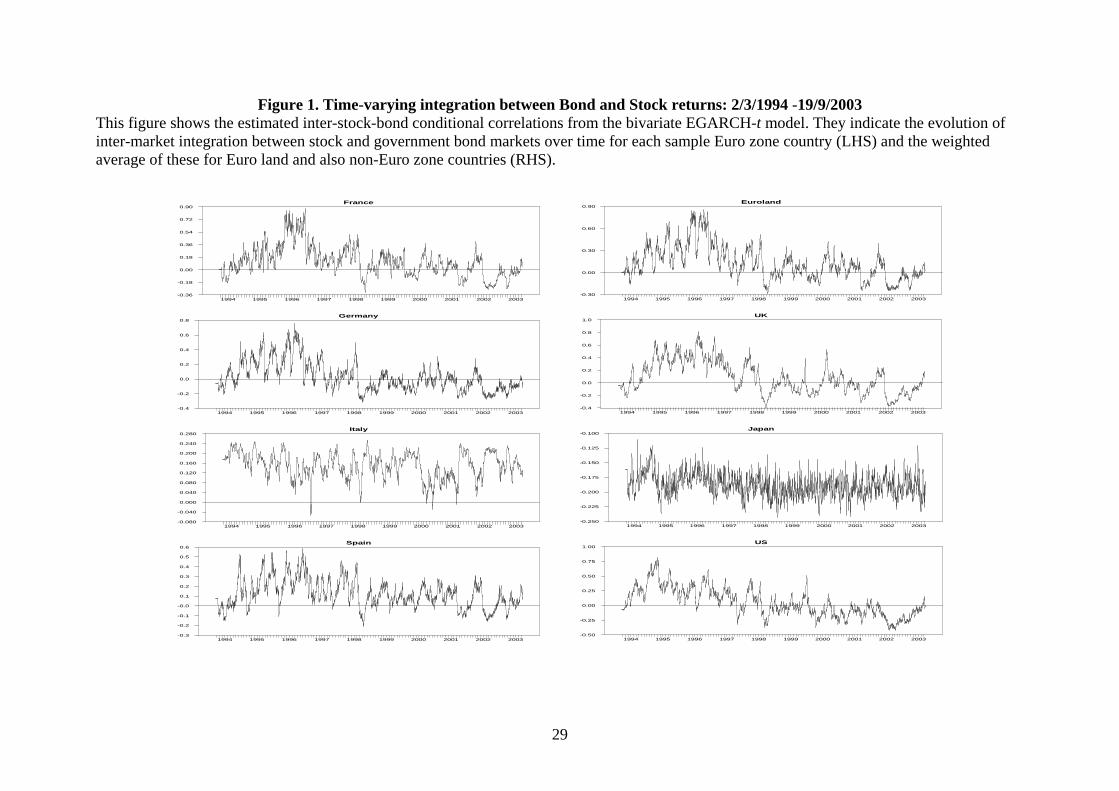
Figure 1 shows the graphs of the estimated dynamic inter-stock-bond conditional

correlations for each sample Euro zone country (on the left-hand column) and the weighted

average of these Euro countries and also non-Euro zone countries (on the right-hand

column).9 There are significant variations in the conditional correlations of stock and bond

returns over the sample period. The most striking conclusion from these graphs is that since

the mid 1990s integration has been falling between these two major financial segments in

Europe and in the rest of the world to zero mean levels (consistent with the behavior of

Cappiello et al.’s, 2003 regional level stock-bond correlations over the same time period),

with the exception in Italy where co-movements between the two markets have been

strengthening since 2000 and Japan where the series has gyrated around a low negative level

(around -0.2). This is new country-level evidence on European cross-market integration as

Cappiello et al. (2003) previously assessed cross-country inter-stock-bond correlations

between Germany, France, Italy and the UK and found strong increases between all EMU

countries around 1999 when the Euro was introduced. This sustained period of inter-stock-

bond market segmentation cannot be attributed to the demise of the tech bubble in the late

1990s as it began earlier in the decade. Instead, it can perhaps be explained in the context of a

flight to quality hypothesis: investors’ uncertainty in the future of the EMU and the

macroeconomic fundamentals under the new exchange rate regime has resulted in investors

flocking to the government bond markets (perceived safe havens) as evidenced by the

declining correlations in bond and stock returns. This is certainly plausible given the poor

economic performance of the larger member countries since the EMU’s inception. However,

9 A caveat of this analysis is the implicit assumption of same risk levels associated with investing in stocks and

government bonds. Hence, the EGARCH model has also been estimated with excess stock returns (risk premia)

to adjust for this and the results are qualitatively similar for most countries.

12

for the historically volatile Italian financial markets, the monetary union has instead been

perceived by investors in the post-Euro time period to reduce macroeconomic uncertainty and

has thus increased co-movements between stock and bond returns. This is supported by

Morana and Beltratti’s (2002) finding that Italy’s stock market volatility has dampened with

the introduction of the Euro. These two explanations are also consistent with the fundamental

approach represented by Campbell and Ammer (1993) in which a differential response to

inflation expectations in the pricing of these two securities may induce low correlations as

inflation is generally viewed as bad news for bonds and ambiguous news for stocks.

Furthermore, consistent with the stylized fact of negative stock and bond return correlations in

times of financial turmoil (eg., see Chordia et al., 2005 and Hartmann et al., 2004) it is not

surprising that Japan exhibits a stable negative correlation level over the sample period given

its enduring financial problems over the sample period. Finally, using stock-bond return

correlations over consecutive periods, Connolly et al. (2005) showed negative correlations

were more likely when stock market uncertainty (ie. economic uncertainty) was high. This

also lends support for our explanations.

Probing further into the EMU’s influence on our observed segmentation trend in

international stock-bond markets, we provide some evidence on how the two individual

financial segments have been integrating with the EMU region in Figure 2. We estimate a

similar bivariate EGARCH-t model with time varying conditional correlations but using

national and value-weighted Euro zone asset returns instead of same country bond and stock

returns.10 Hence, in Figure 2 the historical path of conditional correlations between bond

market returns are shown on the left hand side column (to proxy intra-bond market integration

10 To avoid spurious integration results from the bivariate EGARCH estimations, we generated EMU regional

indices separately for stock and bond markets that excluded individual sample EMU countries in the weighted

average calculation.

13

with the EMU) and those for stock market returns are depicted on the right hand side column

(to proxy intra-stock market integration with the EMU). 11

In Figure 2, it is clear that international stock markets had rapidly integrated with

EMU stock markets in the few years leading up to the introduction of the Euro, corroborating

with Fratzscher’s (2002) and Kim et al.’s (in-press) stock market integration studies and

increases in Cappiello et al.’s (2003) average contemporaneous correlation calculations for

stock markets. However, compared to the series of intra-stock market conditional correlation

charts, those for intra-bond markets are relatively heterogeneous. By construction, the four

Euro zone bond markets are highly correlated with the Euro zone regional bond index return

as evidenced by the extremely high conditional correlation levels (ranging from 0.65 to

almost 1.0). However, the synchronization of monetary policy with the introduction of the

Euro has no doubt also contributed to this. Not surprisingly, outside of the Euro zone the

UK’s government bond market is the most correlated with the core Euro zone market index

(correlations range 0.68 - 0.75), followed by the United States (0.38 - 0.48) and then Japan

(0.03 – 0.09). There has generally been an upward trend in intra-bond market integration with

the core Euro zone in part of the sample period for all sample countries. For the four EMU

countries, bond markets had become integrated even before the stock markets but they appear

to have plateaued from mid 1998. This is consistent with existing European financial market

studies that generally find the single currency had influenced government bond markets in the

EMU even before the Euro was officially launched in 1999 (eg, see Galati and Tsatsaronis,

2003). Outside of the EMU, the UK, US and Japanese bond markets have been slower to

integrate with the EMU but a slight upward trend has emerged as the new exchange rate

regime became imminent. This is also supported by increases in Cappiello et al.’s (2003)

11 The underlying estimation results for intra-market integration with the EMU are not reported here due to space

considerations but are available upon request from the corresponding author.

14

average correlation calculations for bond markets. While international stock and bond markets

have become more intricately linked with the Euro zone markets, this international financial

development has segmented stock and bond markets at the country level. This suggests that

macroeconomic developments associated with the EMU should explain inter-stock-bond

market integration dynamics.

4.2 Estimation results for international stock and bond returns: Volatility linkages

The bivariate estimation results for the EGARCH-t model with volatility spillovers are

shown in Table 2. The coefficients for the lagged conditional variance terms (βhB and βhS) are

very close to one for all pairs of bond and stock market returns indicating a high level of

persistence in shocks to the conditional volatility and hence, the appropriateness of a GARCH

framework.12 The diagnostics for our maximum likelihood estimations are provided at the

bottom of Table 2. The joint conditional t density function assumed for the innovations

converged asymptotically to the Normal distribution as 1/D (D being degrees of freedom) was

very close to zero in all cases.13 The Ljung Box Q statistics show that both univariate and

bivariate serial correlation was successfully removed for all countries, eliminating potential

biases in our estimates. The high level of significance for estimates in the covariance

equations (shown in Table 2) strengthens our confidence in the validity of the conditional

correlation time series illustrated in Figure 1.

Whilst the conditional volatility of stock market returns display significant asymmetric

and volume effects with the appropriate signs for its own return shocks, bond market

conditional volatility generally does not exhibit an asymmetric response to its own

12 As a robustness check, this model was also estimated with the conditional variance included in the mean

equations (EGARCH-M) but these terms were found to be insignificant for most sample countries.

15

unexpected shocks. This is consistent with Scruggs and Glabadanidis (2003) and Cappiello et

al. (2003) but our bivariate EGARCH methodology is better able to quantify both asymmetric

(sign) and volume (magnitude) effects on conditional variances as we can interpret estimated

parameters instead of relying on the shape of news impact surfaces. Fundamentally, our

results are consistent with these previous studies on conditional stock-bond co-movements but

our new findings emanate due to different time periods, sample countries and methodologies

used. Whilst we find conditional stock market volatilities are relatively more responsive to

bond market return shocks than conditional bond market volatilities are to stock market return

shocks, we also find that bond market conditional variances are not completely unresponsive

to stock return shocks. The asymmetric effect is significantly positive for Japan and the US

and the volume effect is significantly negative for Spain and the UK which is contrary to the

well-known findings for stock markets and is a new result with an international aspect. This

pattern in cross-market return shocks is repeated more strongly for conditional stock market

variances. This means that generally, an unexpected rise in one asset market has a bigger

stabilizing effect on the other asset market’s conditional volatility than unexpected falls but

this is offset to some extent by systemic rises in financial market volatility when there is a

shock in either market. This new result on cross-market volatility interdependence supports

the flight to quality hypothesis as it provides indirect evidence that when positive news hits

one asset market, volatility is dampened in the other as investors tend to stick with their asset

allocations but when negative news hits, investors tend to switch towards perceived ‘quality’

investments thereby increasing cross-market volatility.

Furthermore, we find that cross-market volatility spillovers are mostly unilateral for

Euro zone markets in that only shocks in bond returns affect stock market volatility and not

13 A normal log density function was also assumed but there was little difference in the estimates due to the joint

student t log density’s ability to accommodate normal distributions.

16

vice versa. However, for non-Euro financial markets, volatility spillovers are bilateral in that

unanticipated return shocks in both bond and stock markets affect the other. This is another

new finding in our country level study and suggests that common information affects non-

Euro stock and bond markets simultaneously whilst in the Euro zone, information appears to

change expectations in the bond market initially and this is then transmitted to stock markets,

perhaps through portfolio rebalancing. A key explanation for this is the common sensitivity of

EMU bond markets to the official level of interest rates (monetary policy stance) set by the

European Central Bank for all EMU members and this result has clear policy implications.

In Table 2, the coefficients on lagged mean cross-market returns are generally

significant and positive indicating positive return spillover effects between bond and stock

markets. This is also consistent with the flight to quality phenomenon as when stock market

returns fall, investors tend to flock and bid up the price of government bonds and the inverse

relationship with yields will cause a subsequent fall in bond returns to result. Hence, we find

support for the flight to quality explanation for the financial segmentation between stock and

bond markets on the basis of estimated return and volatility linkages in our bivariate

EGARCH-t model. In the rest of this paper, we determine the underlying macroeconomic

forces at play in driving the international stock and bond market integration/segmentation

process over the sample period associated with the formation of the EMU.

5. EMU influence on International Stock-Bond market integration

First, we test for causality between the European currency unification experience and

international stock-bond market integration to facilitate our context and modeling strategy. As

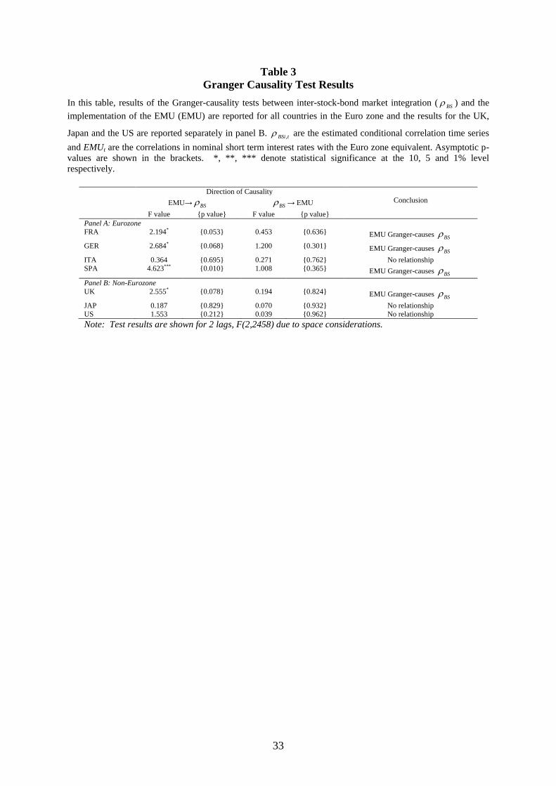
seen in Table 3, there exists uni-directional causality from the EMU to the inter-stock-bond

market integration in only European countries. The Italian stock and bond markets have not

exhibited segmentation dynamics like those in the other Euro zone members and it is

17

interesting that the formation of the EMU has not been necessary for its inter-stock-bond

market developments. The causality result for the UK is largely consistent with the EMU

members and this is not surprising given that they are affected by many common economic

factors. The implications of these results for policy makers is that by conforming with the new

exchange rate regime, they have created improved diversification benefits in international

stock and bond markets as suggested by the causal relationship with the observed declining

integration series.

Our simple analysis provides new findings for inter-market integration both in and

outside of the EMU. Next, we account for the predictive ability of the EMU in the next

section by replacing the EMU proxy with variables adopted from the Optimal Currency Area

(OCA) literature in a seemingly unrelated regression estimation (SURE). It has been

recognized in the literature that what drives time variations in financial market integration

may not be a country’s own fundamentals but also the degree of real and financial

convergence with other economies (see Fratzscher, 2002). The EMU has involved

tremendous convergence on many different macroeconomic facets and these are well captured

by the range of assessment criteria used in Optimal Currency Area (OCA) analyses, some of

which have been applied by Fratzscher (2002) and Baele (2005) to assess European stock

market integration. We extend from this work and conduct principal component analyses for

the broad economic channels through which the EMU may have played a role on financial

market integration: real integration, monetary policy convergence and exchange rate risk

reduction. We expect a priori on the basis of OCA theory that as economies become more

alike, the benefits of a monetary union increases. As Mamaysky (2002) notes, if a given set of

explanatory variables is truly important for determining joint stock-bond returns, they must

represent a risk that is priced in the economy and it is on this ground that these may be

potential determinants of stock-bond integration dynamics.

18

We found a high degree of multicollinearity between the various OCA criteria adopted

in this study. This is not surprising given that the convergence in the real economies and

monetary policies did not occur in isolation during the European currency unification process.

Like Fratzscher (2002) we overcome potentially spurious regression results by forming two

principal components to represent the variables which combine to proxy these two different

facets of economic integration.

We subsequently incorporate these two principal component variables, exchange rate

volatility and a January dummy variable into a pooled cross-sectional time series SURE to

gauge the influence of macroeconomic convergence on dynamic financial market integration.

This is a technique which has not previously been applied to explain bond-stock co-

movements but it makes intuitive sense in our investigation. Our implicit assumption by using

SURE is that the residuals in our system of linear equations are contemporaneously correlated

at any point in time because they are capturing similar omitted factors on each country’s

financial integration process. These may include regulatory barriers, political, institutional,

legal, social and cultural factors, posing additional information normally omitted from

separate OLS estimation. Hence, we make use of the contemporaneous correlation

assumption and jointly estimate a system of seven equations (one for each sample country)

within a generalized least squares (GLS) framework to improve our estimates.14 The SURE

results for the following model are shown in Table 4.15

14 The correlation matrix for residuals from each individual country in the SUR system of equations reveal that

correlations are of sufficient magnitude to warrant SUR over separate least squares estimation. Separate OLS

regressions were run for a comparison and these are available upon request from the authors.

15 a) This model controls for the predictability of integration levels based on Granger causality test results by

including lagged instead of contemporaneous explanatory variables. Information variables (dividend yield -DIV,

short-term interest rate – ST_IRATE and term structure - TERM) have also been used as controls in this

regression model because of their well-known predictive ability for stock and bond returns (see Scruggs and

19

_ _ _, 1 2 , 1 3 , 1 4 , 1

_5 , 6 , 1 7 , 2

EX VOL REAL INT MON INTBSi t i i i t i i t i i t

JAN DUM ui i t i BSi t i BSi t it

ρ α α α α

α α ρ α ρ

= + + +− − −

+ + + +− −

(5)

where the dependent variable ( ,BSi tρ ) is the conditional bond-stock correlation series for each

country i {France, Germany, Italy, Spain, UK, Japan, US}, EX_VOLi,t-1 = lagged conditional

exchange rate volatility, REAL_INT i,t-1 = lagged real economic convergence, MON_INT i,t-1 =

lagged monetary policy convergence and JAN_DUM is the January dummy variable, and

, 1BSi tρ − and , 2BSi tρ − are the first and second lags of the dependent variable.

As with most cross-country studies, there are slight differences with respect to the

significance of the explanatory variables across sample countries in our SUR system.

However, the fact that the three macroeconomic variables of interest are not all significant for

each individual country suggests that we have been successful in orthogonalizing the EMU’s

channels of influence. Firstly, reductions in conditional foreign exchange volatilities have

only been important to bond and stock market interdependencies in Germany and Japan. We

believe this makes intuitive sense given that exchange rates have been required to fluctuate

within narrow bands from a basket of European currencies (ECU) since 1979 and this already

made the Euro a close substitute for the currencies of most European countries. However in

line with our expectations based on OCA theory and Fratzscher’s (2002) stock market

findings, reductions in exchange rate volatility have only been effective in stimulating stock

and bond market integration (and not segmentation) in our sample countries (as indicated by

Glabadanidis, 2003). However, the results are not significantly different without them and we overcome the

problem of multicollinearity as they are used in constructing the macroeconomic convergence principal

components.

b) Augmented Dickey Fuller test statistics on inter-stock-bond integration levels in Table 4 rejected the presence

of a unit root at the conventional 5% level of significance indicating stationarity in all cases.

20

their significant and negative coefficients). The weak contribution of exchange rate risk

reduction to the integration of stock and bond markets is consistent with Bodart and Reding’s

(1999) finding that correlations in stock and bond returns in Europe were not very sensitive to

changes in the Exchange Rate Mechanism and also De Santis et al.’s (2003) finding that

adoption of the Euro did not have a large impact on aggregate currency risk premia. Secondly,

real economic integration also appears to have played a significant role in steering stock and

bond markets towards further integration within the EMU and with Japan and the US

(positive coefficient) as OCA theory would dictate. Thirdly, monetary policy convergence

(inferred from inflation, nominal and real short term interest rates) is only a positively

significant determinant of inter-bond and stock market integration in Italy (where there has

been the only sign of an upward trend in integration between these two financial segments as

Figure 1 revealed). This suggests that a combination of monetary policy changes in the past

decade may be the culprit in inducing investor uncertainty on the future of the EMU thereby

creating a flight to quality investments in other sample countries. We investigated this

possibility further in sub-sample estimations where we found clear negative signs on most

coefficients and in subsequent analysis on economic uncertainty. However, corroborating

with this argument is the finding by Chordia et al. (2005) that co-movements in stock and

bond market liquidity are driven by monetary shocks and also Li’s (2002) empirical results

indicate the major trends in stock-bond correlations are determined by uncertainty on

expected inflation. Fourthly, we find no evidence of seasonality (January or day of the week

effects) in bond and stock market integration dynamics, especially outside of the US. This

finding is not surprising given the amount of mixed evidence on seasonality outside of equity

markets (eg., see Smith, 2002) but this is still a new international result given that calendar

regularities have been found in stock and bond market liquidity by Chordia et al. (2005) using

intraday US data. Finally, we find that stock and bond market integration/segmentation is a

21

persistent process as indicated by the highly significant lagged dependent variable terms for

most sample countries and this is consistent with serial correlations found in stock-bond

correlations by Li (2002).16

A Chow test is conducted to test for structural change in estimated parameters pre- and

post-Euro introduction. The Chow test involved a test of the joint significance of the entire set

of additional interactive dummies in the regression (regressors multiplied by a Euro time

dummy that took the value of one from 1 January 1999 onwards and zero prior to that). The

null hypothesis of no structural change in the estimates was rejected, justifying separate

regressions for a pre- and post-Euro sub-sample period to gauge the changing importance of

the three main economic channels in explaining bond and stock market

integration/segmentation.17 The sample split is informative in that it reveals that the reduction

in exchange rate volatility was effective in fostering European inter-bond and stock market

integration in the lead up to the Euro’s introduction but not since then. On the other hand, real

economic integration has only been stimulatory for inter-stock-bond market integration in the

post-Euro era, as prior to the introduction of the single currency it had generally contributed

to the segmentation of stock-bond markets. As mentioned before, monetary policy

convergence has been a pervasive deterrent to stock-bond market integration as suggested by

the negative coefficients observed in both sub-samples.

16 We present Ljung Box Q tests for serial correlation as it can be used in the presence of lagged dependent

variables without any bias towards the finding of no serial correlation. On the basis of these Q statistics it can be

seen that serial correlation has been successfully removed in most equations with two autoregressive terms.

17 A Euro dummy was also significant in a full sample regression but its omission reduces multicollinearity

between regressors. Sub-sample results have been omitted due to space constraints but are available on request.

22

International Stock-Bond market segmentation and Economic uncertainty

Segmentation between bond and stock markets is now a persistent process in most of

Europe and the rest of the world driven perhaps due to continued uncertainty about the

economic and financial future of the International Monetary System.

In the financial economics literature, implied volatilities are generally accepted as a

good proxy for the time-varying uncertainty associated with the expected future stochastic

stock volatility. Connolly et al. (2005) provides convincing empirical evidence on the

influence of stock market uncertainty measures on time-variations in the co-movements of

stock and government bond returns, motivated by the seminal work of Veronesi (1999) on

time-varying stock market uncertainty being a reflection of economic uncertainty. It is argued

that in a state of higher economic uncertainty, new information may receive higher weighting

in the stock price formation process, leading to time-variations in stock market volatility.

Extending Connolly et al. (2005), we apply a stock market uncertainty measure to

investigate the influence of economic state uncertainty on time-variations in stock and bond

market integration/segmentation dynamics. Thus, we use the CBOE’s Volatility Index (VIX)

and the implied volatility index from the DAX (VDAX) as a proxy for economic uncertainty

in our sample countries and sample period. As an increase in these implied volatility indices

are generally viewed by market participants as a sign of increasing aversion to uncertainty, we

expect a priori a negative relationship between the lagged levels of economic uncertainty and

the integration between stock and bond markets. Hence, we estimate the following model for

each country to investigate the explanatory power of economic uncertainty in driving inter-

stock-bond integration dynamics:

, 1 2 1 3 , 1 4 , 2 ,( )BSi t i i t i BSi t i BSi t i tLn uncertρ β β β ρ β ρ µ− − −= + + + + (6)

where the dependent variable ( ,BSi tρ ) is the conditional bond-stock correlation series for each

country i {France, Germany, Italy, Spain, UK, Japan, US}, Ln(uncertt-1) is the natural

23

logarithm of the lagged implied volatilities from equity index options and , 1BSi tρ − and

, 2BSi tρ − are the first and second lags of the dependent variable to reduce serial correlation.

OLS estimations18 revealed that for all countries except Italy, the coefficient on the

uncertainty variable is negative and significant at the 1% level lending further support to the

account that it is uncertainty on the economic future of the international financial system

which is driving segmentation in international stock and bond markets. In the EMU, the

recent change in exchange rate regime is more than likely to have contributed to the region’s

economic and financial uncertainties but it is clear that its influence reaches internationally.

This is a new interpretation and confirms Connolly et al.’s (2005) results using the US and

other G7 countries, that there is an international aspect to the inverse relationship between

stock market uncertainty and stock-bond market co-movements. Economic uncertainty in the

international monetary system is causing a prolonged flight to quality investments (less

extreme than investor reactions in financial crises) and this is improving diversification

benefits between stocks and bonds at the country level. Italy is the only country where inter-

stock-bond market integration has recently increased and the coefficient on the uncertainty

variable is positively significant suggesting that economic uncertainty associated with the

EMU has not triggered the same response in its bond and stock markets.

6. Conclusions

The aim of this paper is to investigate whether time-varying co-movements between

daily government bond and stock returns over the past decade have been affected by the

implementation of the EMU. We find that as intra-stock and bond market integration with the

EMU has strengthened in the sample period, inter-stock-bond market integration at the

18 The OLS results for equation (6) are available upon request from the corresponding author but have been omitted due to space constraints.

24

country level has trended downwards to zero and even negative mean levels in most European

countries, Japan and the US - consistent with a flight to quality phenomena in international

financial markets. We find further evidence to support this in estimated sign and volume

effects on cross-market volatility spillovers in a bivariate EGARCH model and we note that

bond market return shocks have more influence than stock market shocks consistent with

existing literature. There is convincing evidence that the introduction of the monetary union

has Granger caused the apparent segmentation between bond and stock markets within

Europe but not outside. Moreover, real economic integration with the EMU and reduction in

currency risk with the Euro have generally stimulated inter-financial market integration but

the adoption of a common monetary policy may have brought about investor concerns on the

future of macroeconomic fundamentals in Europe and the international financial system,

inducing a flight to government bonds, a perceived safe haven asset. To this end, the EMU

has increased benefits of diversification across stocks and government bonds at the country

level. There are no clear seasonal patterns in inter-market integration/segmentation dynamics

between daily government bond and stock returns in this international study.

We have made significant contributions to the broad finance literature on many levels,

including i) providing a new application of stock-bond co-movements to proxy inter-financial

market integration over time; ii) illustrating a two-step methodology that is suitable for this

new application; iii) using higher frequency (daily) data to investigate international stock-

bond co-movements; iv) improving understanding on cross-market conditional volatility

interdependencies and correlations at the country level; v) establishing the direction of

causality for inter-financial market integration and monetary union adoption; and vi)

providing an alternative theoretical explanation for stock-bond co-movements by using

macroeconomic convergence criteria associated with optimal currency area studies and

25

reinforced with a robust stock market uncertainty measure to study international inter-stock-

bond market integration.

This paper has important implications for both investors and policy makers. For

investors, inter-stock-bond market segmentation at the country level means that

diversifications benefits have increased for even domestic asset allocations. For policy

makers, the process of monetary policy coordination is creating heightened economic

uncertainty in financial markets and financial system instability may become more

pronounced as asset markets of the same type become more interdependent and asset markets

in the same jurisdiction continue to react to those developments.

26

References

Baele, L., 2005. Volatility Spillover Effects in European Equity Markets. Journal of Financial

and Quantitative Analysis, forthcoming.

Baele, L., Ferrando, A., Hordahl, P., Krylova, E., Monnet, C., 2004. Measuring Financial

Integration in the Euro Area. Occasional Paper 14, European Central Bank.

Barr, D.G., Priestley, R., 2004. Expected returns, risk and the integration of international bond

markets. Journal of International Money and Finance 23(1), 71-98.

Bekaert, G., Harvey, C.R., 1995. Time-varying world market integration. Journal of Finance

50, 403-444.

Bekaert, G., Harvey, C.R., 2003. Emerging markets finance. Journal of Empirical Finance 10,

3-55.

Bodart, V., Reding, P., 1999. Exchange rate regime, volatility and international correlations

on bond and stock markets. Journal of International Money and Finance, 18, 133-151.

Bracker, K., Docking, D., Koch, P., 1999. Economic determinants of evolution in

international stock market integration. Journal of Empirical Finance 6, 1-27.

Campbell, J.Y., Ammer, J., 1993. What moves the stock and bond markets? A variance

decomposition for long-term asset returns. Journal of Finance 48(1), 3-37.

Cappiello, L., Engle, R.F., Sheppard, K., 2003. Asymmetric dynamics in the correlations of

global equity and bond returns. European Central Bank working paper no. 204,

Frankfurt am Main.

Chordia, T., Sarkar, A., Subrahmanyam, A., 2005. An Empirical analysis of stock and bond

market liquidity. Review of Financial Studies 18(1), 85-129.

Connolly, R., Stivers, C., Sun, L., 2005. Stock market uncertainty and the Stock-Bond Return

Relation. Journal of Financial and Quantitative Analysis, forthcoming.

Darbar, S.M., Deb, P., 2002. Cross-market correlations and transmission of information.

Journal of Futures Markets 22(11), 1059-82.

27

De Santis, G., Gerard, B., Hillion, P., 2003. The relevance of currency risk in the European

Monetary Union. International Economics and Business 55, 427-462.

Engle, R. 2002. Dynamic Conditional Correlation—A Simple Class of Multivariate GARCH

Models. Journal of Business and Economic Statistics 20, 339-350.

Engle, R., Ng, V.K., 1993. Measuring and testing the impact of news on volatility. Journal of

Finance 48, 1749-78.

Engsted, T., Tanggaard, C., 2001. The Danish Stock and Bond markets: Comovement, Return

predictability and variance decomposition. Journal of Empirical Finance 8, 243-271.

Fleming, J., Kirby, C., Ostdiek, B., 1998. Information and volume linkages in the stock, bond

and money markets. Journal of Financial Economics 49, 111-137.

Fratzscher, M., 2002. Financial market integration in Europe: On the effects of the EMU on

stock markets. International Journal of Finance and Economics 7, 165-193.

Galati, G., and Tsatsaronis, K., 2003. The impact of the euro on Europe’s financial markets.

Financial Markets, Institutions and Instruments 12(3), 165-221.

Hartmann, P., Straetmans, S., Devries, C., 2004. Asset Market Linkages in Crisis Periods. The

Review of Economics and Statistics 86(1), 313-326.

Ilmanen, A., 1995. Time-varying expected returns in international bond markets. Journal of

Finance 50(2), 481-506.

Karolyi, G.A., Stulz, R.M., 1996. Why do markets move together? An investigation of U.S-

Japan stock return comovements. Journal of Finance 51(3), 951-986.

Kim, S-J., Moshirian, F., Wu, E., (In-Press). Dynamic Stock market integration driven by the

European Monetary Union: An empirical analysis. Journal of Banking and Finance.

Kodres, L., Pritsker, M., 2002. A rational expectations model of financial contagion. Journal

of Finance 57, 769-799.

Kroner, K.F., Ng, V.K., 1998. Modeling asymmetric comovements of asset returns. The

28

Review of Financial Studies 11(4), 817-844.

Li, L., 2002. Macroeconomic factors and the correlation of stock and bond returns. Working

paper, Yale University.

Longin, F., Solnik, B., 1995. Is the correlation in international equity returns constant:1960-

1990? Journal of International Money and Finance 14(1), 3-26.

Mamaysky, H., 2002. Market prices of risk and return predictability in a joint stock-bond

pricing model. Yale International Centre for Finance working paper no. 02-25.

McKinnon, R.I., 1963. Optimum currency areas. American Economic Review, 53,

September, 717-725.

Morana, C., Beltratti, A., 2002. The effects of the introduction of the euro on the volatility of

European Stock markets. Journal of Banking and Finance 26, 2047-2064.

Mundell, R.A., 1961. A theory of optimum currency areas. American Economic Review, 51,

September, 657-65.

Nelson, D.B. (1991). Conditional heteroskedasticity in asset returns: A new approach.

Econometrica 59, 347-370.

Prasad, E., Rogoff, K. Wei, S.-J., Kose, M.A., 2003. The effects of financial globalization on

developing countries: Some empirical evidence. IMF Occasional paper no. 220.

Scruggs, J.T., Glabadanidis, P., 2003. Risk premia and the dynamic covariance between stock

and bond returns. Journal of Financial and Quantitative Analysis 38(2), 295-316.

Smith, K.L., 2002. Government bond market seasonality, diversification, and cointegration:

International evidence. Journal of Financial Research 25(2), 203-221.

Veronesi, P., 1999. Stock market overreaction to bad news in good times: A rational

expectations equilibrium model. The Review of Financial Studies 12, 975-1007.

Wu, G., 2001. The determinants of asymmetric volatility. The Review of Financial Studies

14(3), 837-859.

29

Figure 1. Time-varying integration between Bond and Stock returns: 2/3/1994 -19/9/2003 This figure shows the estimated inter-stock-bond conditional correlations from the bivariate EGARCH-t model. They indicate the evolution of inter-market integration between stock and government bond markets over time for each sample Euro zone country (LHS) and the weighted average of these for Euro land and also non-Euro zone countries (RHS).

France

1994 1995 1996 1997 1998 1999 2000 2001 2002 2003-0.36

-0.18

0.00

0.18

0.36

0.54

0.72

0.90

Germany

1994 1995 1996 1997 1998 1999 2000 2001 2002 2003-0.4

-0.2

0.0

0.2

0.4

0.6

0.8

Italy

1994 1995 1996 1997 1998 1999 2000 2001 2002 2003-0.080

-0.040

0.000

0.040

0.080

0.120

0.160

0.200

0.240

0.280

Spain

1994 1995 1996 1997 1998 1999 2000 2001 2002 2003-0.3

-0.2

-0.1

-0.0

0.1

0.2

0.3

0.4

0.5

0.6

Euroland

1994 1995 1996 1997 1998 1999 2000 2001 2002 2003-0.30

0.00

0.30

0.60

0.90

UK

1994 1995 1996 1997 1998 1999 2000 2001 2002 2003-0.4

-0.2

0.0

0.2

0.4

0.6

0.8

1.0

Japan

1994 1995 1996 1997 1998 1999 2000 2001 2002 2003-0.250

-0.225

-0.200

-0.175

-0.150

-0.125

-0.100

US

1994 1995 1996 1997 1998 1999 2000 2001 2002 2003-0.50

-0.25

0.00

0.25

0.50

0.75

1.00

30

Figure 2. Time varying integration with the EMU in Government Bond (LHS) and Stock (RHS) markets: 2/3/1994 -19/9/2003

This figure illustrates the evolution of intra-market integration with the Euro region for national government bond markets (LHS) and stock markets (RHS) using estimated conditional correlations.

France: Bonds

1994 1995 1996 1997 1998 1999 2000 2001 2002 20030.680

0.720

0.760

0.800

0.840

0.880

0.920

0.960

Germany: Bonds

1994 1995 1996 1997 1998 1999 2000 2001 2002 20030.7750.8000.8250.8500.8750.9000.9250.9500.9751.000

Italy: Bonds

1994 1995 1996 1997 1998 1999 2000 2001 2002 20030.680

0.720

0.760

0.800

0.840

0.880

0.920

0.960

1.000

Spain: Bonds

1994 1995 1996 1997 1998 1999 2000 2001 2002 20030.75

0.80

0.85

0.90

0.95

1.00

UK: Bonds

1994 1995 1996 1997 1998 1999 2000 2001 2002 20030.672

0.688

0.704

0.720

0.736

0.752

Japan: Bonds

1994 1995 1996 1997 1998 1999 2000 2001 2002 20030.03

0.04

0.05

0.06

0.07

0.08

0.09

0.10

US: Bonds

1994 1995 1996 1997 1998 1999 2000 2001 2002 20030.378

0.396

0.414

0.432

0.450

0.468

0.486

France: Stocks

1994 1995 1996 1997 1998 1999 2000 2001 2002 20030.500.550.600.650.700.750.800.850.900.95

Germany: Stocks

1994 1995 1996 1997 1998 1999 2000 2001 2002 20030.450.500.550.600.650.700.750.800.850.90

Italy: Stocks

1994 1995 1996 1997 1998 1999 2000 2001 2002 20030.2

0.3

0.4

0.5

0.6

0.7

0.8

0.9

1.0

Spain: Stocks

1994 1995 1996 1997 1998 1999 2000 2001 2002 20030.3

0.4

0.5

0.6

0.7

0.8

0.9

UK: Stocks

1994 1995 1996 1997 1998 1999 2000 2001 2002 20030.50

0.55

0.60

0.65

0.70

0.75

0.80

0.85

Japan: Stocks

1994 1995 1996 1997 1998 1999 2000 2001 2002 20030.192

0.208

0.224

0.240

0.256

0.272

0.288

0.304

US: Stocks

1994 1995 1996 1997 1998 1999 2000 2001 2002 20030.340

0.345

0.350

0.355

0.360

0.365

0.370

0.375

31

Table 1 Statistical properties of daily bond and equity returns (%), 2/3/1994-19/9/2003

This table presents in panels A and B the summary statistics for the pre- and post-Euro sub-sample periods respectively. Asymptotic p-values are shown in the brackets. *, **, *** denote statistical significance at the 10, 5 and 1% level respectively. Test results for H0:Skewness=0 and H0:Excess kurtosis=0 are indicated. Q(20) is the Ljung-Box test statistic for serial correlation up to the 20th order in the return series; Q2(20) is the Ljung-Box test statistic for serial correlation up to the 20th order in the squared returns. Qb(20) and Q2

b(20) are the bivariate Ljung-Box tests for joint white noise in the linear and squared bond and stock returns up to the 20th order. Bond Index Return Test of univariate iid Stock Index Return Test of univariate iid Test of bivariate iid

Mean return

Variance Skewness Excess Kurtosis

Q(20): χ2(20)

Q2(20): χ2(20)

Mean return

Variance Skewness Excess Kurtosis

Q(20): χ2(20) Q2(20): χ2(20) Qb(20): χ2(80)

Q2b(20):

χ2(80) Panel A: Sub-sample period 1: 2/3/94-31/12/98 FRA 0.046 0.249 -0.256*** 3.493*** 67.812***

{0.000} 524.188***

{0.000} 0.060 1.095 -0.226*** 3.137*** 47.225***

{0.001} 644.323***

{0.000} 110.797**

{0.013} 1261.283***

{0.000} GER 0.044 0.264 -0.703*** 3.760*** 54.657***

{0.000} 251.885***

{0.000} 0.062 1.077 -0.867*** 5.381*** 81.866***

{0.000} 845.385***

{0.000} 142.528***

{0.000} 1095.219***

{0.000} ITA 0.078 0.430 -0.820*** 4.877*** 52.439***

{0.000} 138.287***

{0.000} 0.070 1.976 -0.094 2.157*** 50.538***

{0.000} 655.480***

{0.000} 93.504 {0.143}

900.643*** {0.000}

SPA 0.061 0.261 -0.482*** 3.733*** 79.233*** {0.000}

325.431*** {0.000}

0.090 1.369 -0.561*** 4.205*** 84.546*** {0.000}

936.326*** {0.000}

168.617*** {0.000}

1397.832*** {0.000}

EMU• 0.058 0.220 -0.694*** 3.025*** 84.056*** {0.000}

166.973*** {0.000}

0.068 0.922 -0.637*** 5.097*** 95.543*** {0.000}

1124.467*** {0.000}

187.665*** {0.000}

1336.299*** {0.000}

UK 0.050 0.267 -0.355*** 3.959*** 38.916*** {0.007}

143.838*** {0.000}

0.056 0.629 -0.227*** 2.500*** 52.017*** {0.000}

1208.309*** {0.000}

112.953*** {0.009}

1355.691*** {0.000}

US 0.039 0.288 -0.291*** 1.534*** 35.606** {0.017}

60.104*** {0.000}

0.088 0.769 -0.759*** 8.737*** 31.309* {0.051}

302.357*** {0.000}

75.673 {0.616}

385.556*** {0.000}

JAP 0.034 0.132 -0.825*** 7.256*** 61.743*** {0.000}

261.910*** {0.000}

-0.025 1.133 0.251*** 3.810*** 41.131*** {0.004}

361.192*** {0.000}

119.711*** {0.003}

629.910*** {0.000}

Panel B: Sub-sample period 2: 1/1/99-19/9/03 FRA 0.019 0.225 -0.327*** 1.374*** 26.600

{0.147} 97.131***

{0.000} 0.006 2.262 -0.056 1.575*** 36.789**

{0.012} 689.908***

{0.000} 245.951***

{0.000} 1663.977***

{0.000} GER 0.019 0.288 -0.273*** 1.109*** 31.182*

{0.053} 96.063***

{0.000} -0.018 2.109 -0.084 1.211*** 36.631**

{0.013} 528.853***

{0.000} 164.583***

{0.000} 1308.812***

{0.000} ITA 0.020 0.251 -0.315*** 1.371*** 31.628**

{0.047} 147.812***

{0.000} -0.009 1.850 -0.170** 2.355*** 30.726*

{0.059} 515.490***

{0.000} 155.836***

{0.000} 1378.411***

{0.000} SPA 0.020 0.194 -0.347*** 1.342*** 29.678*

{0.075} 110.416***

{0.000} -0.009 1.852 0.010 1.220*** 24.010

{0.242} 547.439***

{0.000} 128.812***

{0.000} 1428.634***

{0.000} EMU• 0.019 0.243 -0.315*** 1.142*** 31.441**

{0.050} 116.862***

{0.000} -0.005 1.844 -0.106 1.568*** 35.882**

{0.016} 610.903***

{0.000} 149.452***

{0.000} 1524.872***

{0.000} UK 0.014 0.238 -0.115 0.480*** 32.796**

{0.036} 37.010** {0.012}

-0.008 1.505 -0.174** 1.761*** 56.114*** {0.000}

904.504*** {0.000}

190.468*** {0.000}

1959.335*** {0.000}

US 0.024 0.349 -0.455*** 0.756*** 17.218 {0.639}

80.426*** {0.000}

-0.009 1.856 0.125* 1.425*** 26.950 {0.137}

232.404*** {0.000}

123.713*** {0.001}

698.711*** {0.000}

JAP 0.019 0.225 -0.729*** 5.982*** 48.229*** {0.000}

501.105*** {0.000}

0.004 1.720 -0.159** 1.519*** 26.980 {0.136}

66.161*** {0.000}

170.321*** {0.000}

1204.029*** {0.000}

•Stock and bond market returns for the entire EMU are calculated as the value weighted average return of the 4 sample Euro zone markets. The weights used for stock and bond returns are stock market capitalization values from Datastream and annual government gross liabilities sourced from the OECD respectively

32

Table 2 Bivariate-ARMA-EGARCH-t Model Estimations for bond and stock returns with

conditional volatility spillovers In this table, the results of the bivariate EGARCH estimations are reported. The bivariate EGARCH model for each country, as defined in equations (1a,b) and (2a,b) is:

, , , , , , , , * , * , * , * ,1 1 * 1 * 1

; S SB Bp qq p

B t B rS i S t i B j B t j B t S t S rB i B t i S j S t j S ti j i j

R R m R R mα α ε ε α α ε ε− − − −= = = =

= + + + = + + +∑ ∑ ∑ ∑ (1a,b)

, 1 , 1 , 1 , 1, , 1 1 2 1 2

, 1 , 1 , 1 , 1

| | | |2 2ln ln ,B t B t S t S tB t cB hB B t B B S S

B t B t S t S t

h hh h h hε ε ε ε

β β βε βε β βπ π

− − − −−

− − − −

= + + + − + + −

(2a)

, 1 , 1 , 1 , 1, , 1 1 2 1 2

, 1 , 1 , 1 , 1

| | | |2 2ln ln S t S t B t B tS t cS hS S t S S B B

S t S t B t B t

h hh h h hε ε ε ε

β β βε βε β βπ π

− − − −−

− − − −

= + + + − + + −

(2b)

Eurozone Non-Eurozone FRA GER ITA SPA EMU UK JAP US Mean: RB αB 0.041***

{0.000} 0.044*** {0.000}

0.052*** {0.000}

0.051*** {0.000}

0.047*** {0.000}

0.040*** {0.000}

0.038** {0.011}

0.040*** {0.000}

αrS 0.008 {0.174}

0.013** {0.015}

0.034*** {0.001}

-0.141 {0.196}

0.020*** {0.003}

-0.003 {0.728}

0.002 {0.669}

0.023** {0.035}

PS 4 1 1 1 4 1 1 1 QB 5 1 1 1 1 1 1 1 Vol.:RB βcB -0.084

{0.101} -0.041** {0.014}

-0.015 {0.415}

-0.057** {0.024}

-0.076*** {0.003}

-0.057*** {0.000}

-0.070*** {0.000}

-0.012 {0.254}

βhB 0.943*** {0.000}

0.967*** {0.000}

0.980*** {0.000}

0.963*** {0.000}

0.950*** {0.000}

0.958*** {0.000}

0.963*** {0.000}

0.988*** {0.000}

βεB1 -0.006 {0.686}

0.010 {0.493}

-0.003 {0.884}

-0.005 {0.672}

0.001 {0.962}

0.015 {0.183}

-0.008 {0.458}

0.026** {0.026}

βεB2 0.097** {0.042}

0.121*** {0.000}

0.138*** {0.002}

0.127*** {0.008}

0.116*** {0.000}

0.101*** {0.000}

0.226*** {0.000}

0.062*** {0.000}

ΒS1 0.017 {0.305}

-0.014 {0.335}

-0.017 {0.476}

-0.008 {0.634}

0.002 {0.849}

-0.002 {0.897}

0.060*** {0.000}

0.032** {0.014}

ΒS2 -0.008 {0.710}

0.002 {0.942}

0.045 {0.210}

-0.034* {0.057}

-0.023 {0.157}

-0.063*** {0.003}

-0.002 {0.914}

-0.015 {0.354}

Mean:RS αS 0.044**

{0.034} 0.021* {0.082}

0.029 {0.343}

0.048** {0.014}

0.020** {0.042}

0.027** {0.030}

-0.032 {0.144}

0.043*** {0.000}

αrB -0.010 {0.634}

0.179*** {0.000}

0.029 {0.280}

0.189 {0.152}

0.042* {0.078}

0.025 {0.198}

-0.053 {0.248}

0.066*** {0.003}

PB 4 1 1 1 2 1 1 1 QS 0 1 1 1 1 1 1 1 Vol.: RS βCS 0.001

{0. 229} 0.005*** {0.000}

0.022*** {0.000}

0.001 {0.199}

0.001 {0.123}

-0.002* {0.070}

0.010** {0.042}

-0.001 {0.573}

βhS 0.989*** {0.000}

0.981*** {0.001}

0.962** {0.000}

0.993*** {0.000}

0.990*** {0.000}

0.994*** {0.000}

0.982*** {0.000}

0.992*** {0.000}

βεS1 -0.037*** {0.000}

-0.072*** {0.000}

-0.050*** {0.000}

-0.025*** {0.000}

-0.044*** {0.000}

-0.066*** {0.000}

-0.057** {0.000}

-0.074 {0.155}

βεS2 0.089*** {0.000}

0.169*** {0.000}

0.204*** {0.000}

0.065*** {0.000}

0.121*** {0.000}

0.076*** {0.000}

0.113*** {0.000}

0.062*** {0.000}

ΒB1 -0.009** {0.045}

0.004 {0.669}

0.006 {0.608}

0.022*** {0.000}

0.019*** {0.000}

0.027*** {0.000}

0.005 {0.719}

0.019** {0.011}

ΒB2 -0.079*** {0.000}

-0.012 {0.512}

-0.014 {0.598}

-0.053*** {0.000}

-0.056*** {0.000}

-0.032*** {0.000}

0.035** {0.019}

-0.062*** {0.000}

Covariance δ0 0.031***

{0.000} 0.084*** {0.000}

-0.061 {0.282}

0.171*** {0.000}

0.207*** {0.000}

0.374*** {0.000}

0.005 {0.716}

0.599*** {0.000}

δ1 -0.054*** {0.000}

-0.161*** {0.000}

0.258*** {0.000}

0.473** {0.038}

0.393*** {0.000}

-0.832*** {0.001}

-0.158*** {0.000}

-1.070* {0.072}

δ2 0.952*** {0.000}

0.595*** {0.000}

0.004 {0.981}

0.401*** {0.000}

0.333*** {0.000}

-0.248*** {0.000}

0.256 {0.108}

-0.143 {0.355}

Diagnostics D 2321.467***

{0.000} 2029.673*** {0.000}

176.446*** {0.000}

357.304*** {0.000}

3403.337*** {0.000}

8724.01*** {0.005}

41.910*** {0.000}

5443.852*** {0.000}

-Ln L 5253.529 5385.608 5998.695 5191.258 4901.651 4741.537 4670.389 5340.717 Qb(10): χ2(40) 36.664

{0.621} 28.450 {0.914}

46.172 {0.232}

29.640 {0.885}

34.874 {0.700}

49.125 {0.153}

43.460 {0.326}

25.080 {0.969}

Q2b(10):

χ2(40) 24.361 {0.121}

30.391 {0.864}

34.897 {0.699}

49.947 {0.135}

35.845 {0.216}

32.400 {0.798}

17.131 {0.999}

45.467 {0.255}

Notes: D is the degree of freedom in a student t distribution for the two joint error processes. -Ln L is the negative estimated value of log-likelihood. P-Values are shown in the brackets.*,**,*** denote significance at the 10%, 5% and 1% level respectively. Qb(10) and Q2

b(10) are the bivariate Ljung-Box Q tests for joint white noise in the linear and squared standardized residuals (zt’s and z2

t’s) up to the 10th order.

33

Table 3 Granger Causality Test Results

In this table, results of the Granger-causality tests between inter-stock-bond market integration ( BSρ ) and the implementation of the EMU (EMU) are reported for all countries in the Euro zone and the results for the UK,

Japan and the US are reported separately in panel B. ,BSi tρ are the estimated conditional correlation time series and EMUt are the correlations in nominal short term interest rates with the Euro zone equivalent. Asymptotic p-values are shown in the brackets. *, **, *** denote statistical significance at the 10, 5 and 1% level respectively.

Direction of Causality EMU→ BSρ BSρ → EMU Conclusion

F value {p value} F value {p value} Panel A: Eurozone FRA 2.194* {0.053} 0.453 {0.636} EMU Granger-causes BSρ GER 2.684* {0.068} 1.200 {0.301} EMU Granger-causes BSρ ITA 0.364 {0.695} 0.271 {0.762} No relationship SPA 4.623*** {0.010} 1.008 {0.365} EMU Granger-causes BSρ Panel B: Non-Eurozone UK 2.555* {0.078} 0.194 {0.824} EMU Granger-causes BSρ JAP 0.187 {0.829} 0.070 {0.932} No relationship US 1.553 {0.212} 0.039 {0.962} No relationship Note: Test results are shown for 2 lags, F(2,2458) due to space considerations.

34

Table 4 Regression results for the sample period 1/4/1994 to 19/9/2003

In this table, the seemingly unrelated regression (SUR) estimates are shown. The model estimated is defined in equation (5):

_ _ _ _, 1 2 , 1 3 , 1 4 , 1 5 , 6 , 1 7 , 2EX VOL REAL INT MON INT JAN DUM uBSi t i i i t i i t i i t i i t i BSi t i BSi t itρ α α α α α α αρ ρ= + + + + + + +− − − − −

(5)

where the dependent variable ( ,BSi tρ ) is the estimated conditional correlation series for each country i, EX_VOLi,t-1 = lagged conditional exchange rate volatility, REAL_INT i,t-1 = lagged real economic convergence, MON_INT i,t-1 = lagged monetary policy convergence and JAN_DUM is the January dummy variable, and

, 1BSi tρ − and , 2BSi tρ − are the first and second lags of the dependent variable. Euro zone Non-euro zone FRA GER ITA SPA UK JAP US CONSTANT 0.0112***

{0.0067} 0.0113*** { 0.0028}

0.0046*** {0.0000}

0.0064** {0.0199}

-0.0002 {0.9520}

-0.0402*** {0.0000}

0.0011 {0.5991}

EX_VOLt-1 -0.0024 {0.1368}

-0.0035* {0.0520}

-0.0005 {0.3557}

0.0009 {0.5925}

0.0024 {0.2410}

-0.0027*** {0.0000}

0.0029 {0.4753}

REAL_INT t-1 0.0060** {0.0456}

0.0036 {0.1426}

0.0009** {0.0176}

0.0022 {0.2144}

0.0004 {0.8493}

0.0010** {0.0167}

0.0023* {0.0898}

MON_INTt-1 -0.0015 {0.3644}

0.0017 {0.1933}

0.0006* {0.0666}

0.0003 {0.7315}

0.0001 {0.9313}

-0.0003 {0.3137}

0.0009 {0.3904}

JAN_DUM -0.0012 {0.6931}

0.0007 {0.8317}

0.0009 {0.1929}

-0.0017 {0.4833}

-0.0006 {0.7956}

0.0004 {0.6202}

-0.0040 {0.1736}

, 1BSi tρ − 1.0924*** {0.0000}

0.7179*** {0.0000}

1.2900*** {0.0000}

0.8417*** {0.0000}

1.1365*** {0.0000}

0.7397*** {0.0000}

0.8599*** {0.0000}

, 2BSi tρ − -0.1276*** {0.0000}

0.2460*** {0.0000}

-0.3162*** {0.0000}

0.1222*** {0.0000}

-0.1508*** {0.0000}

0.0315 {0.1122}

0.1218*** {0.0000}

Adj. R2 0.9652 0.9533 0.9688 0.9467 0.9857 0.6211 0.9745 ADF Test Statistic -5.5404** -5.4901** -6.4788** -5.7078** -4.2833** -13.1336** -5.6143** Q Test (~χ2

20) 42.1518*** {0.0026}

21.4509 {0.3710}

14.0052 {0.8302}

21.1950 {0.3859}

19.7899 {0.4711}

37.5019** {0.0102}

41.6225*** {0.0031}

Chow test (~χ27) 15.3671**

{0.0316} 30.3336*** {0.0001}

27.3391*** {0.0003}

8.7813 {0.2687}

13.0759* {0.0703}

68.5809*** {0.0000}

19.9231*** {0.0057}

No. obs. 2469 2469 2469 2469 2469 2469 2469 Notes: P values are shown in brackets and *,**,*** denote significance at the 10%, 5% and 1% level respectively. The ADF test included a constant, trend and 4 lags and the critical value at the 5% significance level for the null hypothesis of a unit root is -3.410. The Ljung Box Q test is for a null hypothesis of no serial correlation up to the 20th order. The Chow test is for a null hypothesis of no structural change from the 1st January, 1999.

35

Appendix A Variable Definitions and Data Sources

Category Variable Frequency Source Definition Exchange Rate risk EX_VOL Daily Datastream Conditional variance from a GARCH(1,1)

model for daily local currency to Euro exchange returns.

EX_SD* Daily Datastream Rolling standard deviations of daily changes in the foreign exchange rate over the past 3 months (quarter).

Real Convergence OUTPUT Monthly IMF/Eurostat Rolling correlations in annual growth rates of seasonally adjusted industrial production (IP) with the Euroarea equivalent (weighted by annual GDP share prior to Jan. 1999) over the past 3 months (quarter).

TERM_STRUC Daily Datastream Rolling correlations in the term structure changes (long-term benchmark rates - 1 month LIBOR rates) with Euro area equivalent (weighted by annual GDP share prior to Jan. 1999) over the past 3 months (quarter).

DIV_YIELD Daily Datastream Rolling correlations for changes in dividend yields with the Euro area equivalent (weighted by stock market capitalization) over the past 3 months (quarter).

TRADE_OPEN Monthly Datastream/IMF Ratio of total exports plus imports to annual GDP

TRADE_INT Monthly Datastream Ratio of exports plus imports to/from EMU/EU to total trade

Monetary Policy Convergence

NOM_SRATE Daily Datastream and IMF Rolling correlations in nominal short-term interest rates (1 month LIBOR rates) with the Euro area equivalent (weighted by annual GDP share prior toJan.1998) over the past 3 months.

INFLA Monthly Datastream and IMF

Rolling correlations in seasonally-adjusted consumer price inflation with the Euro-area equivalent (weighted by annual GDP prior to Jan.1998) over the past 3months.

REAL_SRATE Monthly Datastream and IMF Rolling correlations in real short-term interest rates (1 month LIBOR rates - inflation) with the Euro area equivalent (weighted by annual GDP share prior to Jan. 1998).

Control FRI_DUM* Daily Indicator is equal to one if that trading day was a Friday, zero otherwise.

MON_DUM* Daily Indicator is equal to one if that trading day was a Monday, zero otherwise.

JAN_DUM Daily Indicator is equal to one if that trading day was in January, zero otherwise.

EURO_DUM*,** Daily Indicator takes a value of one if the Euro has already been introduced on the date ie. from 1st January 1999 onwards, zero otherwise.

DIV* Daily Datastream Dividend yield levels used to construct DIV_YIELD.

ST_IRATE* Daily Datastream Nominal short-term interest rates used to construct NOM_SRATE.

TERM* Daily Datastream Term spreads used to construct TERM_STRUC.

Economic Uncertainty

UNCERT Daily Datastream Natural logarithm of implied volatilities from equity options index from the Chicago Board of Options Exchange and the German DAX.

* These variables have not been shown in the final model to minimize multicollinearity problems. **Used for

the Chow test.