corporate stock and bond return correlations and dynamic
TRANSCRIPT

This article has been accepted for publication and undergone full peer review but has not been through the copyediting,
typesetting, pagination and proofreading process, which may lead to differences between this version and the Version of
Record. Please cite this article as doi: 10.1111/jbfa.12114.
This article is protected by copyright. All rights reserved. 1
Corporate stock and bond return correlations and dynamic
adjustments of capital structure
This version: December 2014
ABSTRACT
This paper analyses the effects of dynamic correlations between stock and bond returns
issued by the same firm on the speed of adjustment towards target leverage. The results show
that the estimated correlations are time varying, show persistence, and differ among firms.
Analysis of the potential explanatory variables reveals that the correlations decrease with
negative expectations about future aggregate risks, but only for firms with a low default
probability. In contrast, correlations are positively associated with specific risk measures,
especially idiosyncratic stock risk and financial leverage. The positive relation between the
correlations and the leverage ratio suggests that target leverage can be achieved faster when
the stock–bond correlation is high. Our results show that this is the case.
JEL Classification: G32, G12, G14
Keywords: Individual stock–bond correlation, leverage, idiosyncratic risk, economic cycles,
speed of adjustment, target capital structure.

This article is protected by copyright. All rights reserved. 2
1. Introduction
Capital structure choices are one of the most important issues in corporate finance. From the
trade-off theory perspective, firms optimally choose their capital structure to maximize the
net benefits of debt. The benefits of debt come from tax savings (Modigliani and Miller,
1963) and the potential information that debt generates (Harris and Raviv, 1990; Stulz, 1990),
while the costs include basically the expected losses of bankruptcy (Scott, 1976; Titman,
1984) and agency costs (Jensen and Meckling, 1976; Myers, 1977; Jensen, 1986). Empirical
tests of the trade-off theory have consisted in evaluating cross-sectional relations between
leverage ratios and firm characteristics which are used to proxy for both debt benefits and
costs. Another way to test the implications of the trade-off theory is to examine whether firms
actually have target leverage ratios or whether they rebalance their capital structure when
they depart from their target.
Our paper contributes to this literature by showing that the firm’s adjustment towards
its target leverage ratio is faster when the correlation between the returns of stocks and bonds
issued by the firm is higher. Of course, this empirical result can only be understood if we
assume that i) the firm stock–bond correlation is not zero but, rather, time varying and
differing across firms, ii) the stock–bond correlation is related to firm characteristics that are
also relevant to capital structure decisions, and iii) changes in the market value of leverage
are faster if both market debt and equity respond simultaneously to common sources of risk.
Therefore, the goal of this paper is twofold. First, we estimate dynamic individual stock–bond
correlations and analyse which variables can explain their variability both in time series and
cross-sectionally. Second, we estimate a model for leverage adjustments towards the target in
which the speed of adjustment is modelled as a function of the stock–bond correlation.
The correlation in stock and bond markets has been widely investigated at the
aggregate level.1 However, research papers on the comovements between stocks and
corporate bonds at the firm level are scarce. With the theoretical support of structural models
that assume that equity and debt are contingent claims written on the same productive assets,
some empirical studies analyze whether a variable related to one security is relevant in
1 Although primary studies find a small but positive long-term correlation between stocks and Treasury bonds,
the equity and bond markets have behaved very differently since the late 1990s, showing time-varying
behaviour, with positive values in stable periods that decrease meaningfully during recessions (e.g. Gulko, 2002;
Illmanen, 2003; Connolly, Stivers, and Sun, 2005; d’Addona and Kind, 2006; Baele, Bekaert, and Inghelbrecht,
2010).

This article is protected by copyright. All rights reserved. 3
determining a characteristic about the other security.2 We also relay on structural models to
justify a non-zero stock–bond correlation that varies in time and with firm value. For all firms
in the Standard and Poor’s (S&P) 100 Index and with transaction bond prices available in the
Trading Reporting and Compliance Engine (TRACE) database, we estimate dynamic
correlations between individual stock and bond returns using three alternative methodologies:
a rolling sample correlation, a dynamic conditional correlation (DCC) model such as Engle’s
(2002), and a corrected version of the DCC model that incorporates a non-synchronous
trading adjustment that follows the initial proposal of Engle, Kane, and Noh (1996). Our
results suggest that the correlations are, on average, small but very different, depending on
the stock–bond pair, and are time varying, showing persistence.
Using panel data regression, we investigate the sources of variation behind the
correlations dynamics in both the cross-sectional and time series dimensions, considering a
large set of explanatory variables that includes cycle indicators, firm characteristics, or
specific bond contract characteristics. On the one hand, structural models imply that equity
and bond returns are related by ratio of equity elasticity to bond elasticity with respect to
changes in firm value. This relation, which is positive on average, is composed of the ratio
between equity and debt sensitivities to firm value and of the firm leverage ratio. Both these
components vary with firm characteristics, especially those related to risk. Therefore, the
final effect on the correlation is undetermined a priori. On the other hand, intertemporal asset
pricing models recognise the importance of macroeconomic factors in explaining the prices
of both securities. However, empirical results on relative response to changes in economic
conditions are not available. Unique empirical insights come from the works of Campello,
Cheng, and Zhang (2008), Elkamhi and Ericsson (2008), and Schaefer and Strebulaev (2008).
All these papers assume Merton’s (1974) model to show that equity–bond elasticity (equity–
bond return covariance) increases with the quasi-leverage ratio, firm volatility, and time to
maturity. Our analysis of the potential determinants of the variability of stock–bond
correlations indicate that the correlations do not respond to cycle indicators related to
macroeconomic growth but, rather, diminish when negative expectations are measured with
aggregate risk indicators, such as the volatility of consumption growth or the default spread.
2 On the one hand, the effect of the volatility of equity on the bond price has been extensively analyzed
(Campbell and Taskler, 2003; Cremers, Driessen, Maenhout, and Weinbaum, 2008; Zhang, Zhou, and Zhu,
2009). On the other hand, and in the opposite direction, the effect of bond rating changes on stock returns has
also received great attention (e. g. Holthausen and Leftwich, 1986; Barron, Clare, and Thomas, 1997; Abad-
Romero and Robles, 2006).

This article is protected by copyright. All rights reserved. 4
In addition, the correlation diminishes as the systematic stock risk (market beta) increases.
Hence, bonds and stocks of the same firm become increasingly different the greater the
uncertainty in the overall economy and the higher the stock’s systematic risk. However, these
associations are weaker or even disappear when the firm’s default probability is high. In
contrast, the correlation increases with the firm’s specific risk. In particular, the stock–bond
correlation is consistent and strongly associated with the firm’s idiosyncratic stock risk and
financial leverage.
The cross-sectional positive association between the leverage ratio and the stock–
bond correlation is consistent with the theoretical foundations of the structural models. Their
positive time series relation can also be theoretically justified by models assuming agency
costs. Models in line with that of Harris and Raviv (1990) or Stulz (1990) point out the
benefits of debt in reducing information asymmetry, thus supporting a positive relation
between leverage and firm value. Given that we are assuming that both market debt and
equity respond in the same direction to changes in firm value and our empirical results
support this assumption, the higher the correlation, the stronger the effect of firm value
changes on the leverage ratio. Consequently, changes in capital structure towards the target
leverage will be more effective for firms and periods showing high values in the stock–bond
correlation. The final analysis in this paper involves the role of the correlation on the dynamic
adjustment of capital structure. The literature on capital structure concurs on the dynamic
rebalancing of leverage towards the target but differs about the speed of adjustment, which
range from the slow adjustment of Fama and French (2002) to 35 percent annually for
Flannery and Rangan (2006). The speed depends on the firm’s access to capital markets,
financial constraints, and macroeconomic conditions (e.g. Drobetz and Wanzenried, 2006;
Drobetz, Pensa, and Wanzenried, 2007; Cook and Tang, 2010; Faulkender, Flannery,
Hankins, and Smith, 2012). Our contribution relays on the use of the correlation as the
variable informing about specific firm characteristics and market conditions. Then, we
assume a leverage adjustment model in which the target leverage is defined by standard firm
characteristics but the adjustment speed changes with the stock–bond correlation. Estimation
of the model indicates that the speed of adjustment is positive and significantly related to the
correlation. Therefore, when the market values of equity and debt react in the same direction
after news of capital restructuration, the leverage objective can be achieved earlier.
The remainder of the paper is organized as follows. Section 2 theoretically justifies a
non-zero correlation between bond and stock returns and point outs potential determinants of

This article is protected by copyright. All rights reserved. 5
its variation. Section 3 describes the data. Section 4 explains the methodologies and the
results for the dynamic estimation of the correlations. Section 5 analyses the determinants of
stock–bond correlations. Section 6 studies the role of stock–bond correlations in revising
deviations of firm leverage from the target capital structure. Section 7 presents our
conclusions.
2. Theoretical bases
Structural (or dynamic) models are used for capital structure decisions and incorporate the
idea of risky corporate debt. Starting with Merton’s (1974), these models are based on the
fact that the value of the equity and debt of the same firm can be written as functions of firm
value. Therefore, these values (and thus their returns) must be correlated. More specifically,
let B be the market value of the debt of firm j that promises to pay D on date T and let S be
the market value of the same firm’s equity. Suppose that both values can be written as a
function of the firm’s value, V, at time t:
𝑆𝑗𝑡 = 𝑓(𝑉𝑗𝑡, 𝑡); 𝐵𝑗𝑡 = 𝐹(𝑉𝑗𝑡, 𝑡). (1)
Any change in firm value will affect both the equity and debt value as
𝑑𝑆𝑗𝑡
𝑑𝑉𝑗𝑡= 𝑓𝑉(𝑉𝑗𝑡, 𝑡) and
𝑑𝐵𝑗𝑡
𝑑𝑉𝑗𝑡= 𝐹𝑉(𝑉𝑗𝑡 , 𝑡) (2)
where the subscripts in f and F denote partial derivatives.
We can transform the equations in (2) to obtain the return on equity, 𝑅𝑗𝑡𝑆 , and the
return on debt, 𝑅𝑗𝑡𝐵 , respectively:
𝑑𝑆𝑗𝑡
𝑆𝑗𝑡=𝑓𝑉(𝑉𝑗𝑡,𝑡)𝑑𝑉𝑗𝑡
𝑆𝑗𝑡𝑉𝑗𝑡𝑉𝑗𝑡 ↔ 𝑅𝑗𝑡
𝑆 =𝑓𝑉(𝑉𝑗𝑡,𝑡)
𝑆𝑗𝑡𝑅𝑗𝑡𝑉𝑉𝑗𝑡 (3)
𝑑𝐵𝑗𝑡
𝐵𝑗𝑡=𝐹𝑉(𝑉𝑗𝑡,𝑡)𝑑𝑉𝑗𝑡
𝐵𝑗𝑡𝑉𝑗𝑡𝑉𝑗𝑡 ↔ 𝑅𝑗𝑡
𝐵 =𝐹𝑉(𝑉𝑗𝑡,𝑡)
𝐵𝑖𝑗𝑅𝑗𝑡𝑉𝑉𝑗𝑡 (4)
where 𝑅𝑖𝑡𝑉 represents the return on firm value. Combining (3) and (4), we obtain
𝑅𝑗𝑡𝑆 =
𝑓𝑉(𝑉𝑗𝑡,𝑡)
𝐹𝑉(𝑉𝑗𝑡,𝑡)
𝐵𝑗𝑡
𝑆𝑗𝑡𝑅𝑗𝑡𝐵 (5)
which says that the equity and bond returns are related by the equity–bond elasticity with
respect to changes in firm value, supporting the idea of non-zero correlations. The elasticity is

This article is protected by copyright. All rights reserved. 6
composed of the ratio between equity and debt sensitivities to firm value and of the firm
leverage ratio. Additionally, the elasticity is time varying and depends on firm characteristics.
The specific relation between stock and bond returns requires conditions that allow
the specification of the functional form of the elasticity in (5). Under the simplest structural
model, Merton’s (1974), the assumption that firm value follows a diffusion process with
constant instantaneous volatility and standard Brownian motion implies that the sensitivities
ratio is
𝑓𝑉(𝑉𝑗𝑡,𝑡)
𝐹𝑉(𝑉𝑗𝑡,𝑡)=
𝑓𝑉(𝑉𝑗𝑡,𝑡)
(1−𝑓𝑉(𝑉𝑗𝑡,𝑡))=
𝜙(𝑥𝑗𝑡)
1−𝜙(𝑥𝑗𝑡) (6)
where 𝜙 is the cumulative standard normal distribution at
𝑥j𝑡 = [𝑙𝑜𝑔 (𝑉𝑗𝑡 𝐷𝑗) + (𝑟𝑡 + (𝜎𝑗2 2)⁄ )𝜏⁄ ]/𝜎𝑗√𝜏, r is the risk-free rate, σ is the volatility of firm
returns, and 𝜏 = 𝑇 − 𝑡 is the time until the maturity of the debt. Since the leverage ratio
cannot be negative, this model predicts a positive correlation between bond and equity returns
that depends on the variables that determine 𝜙(𝑥𝑗𝑡). Empirically, Campello, Cheng, and
Zhang (2008), Elkamhi and Ericsson (2008), and Schaefer and Strebulaev (2008) find that
Merton’s model implies equity–bond elasticity (equity–bond return covariance) increasing
with the quasi-leverage ratio, firm volatility, and time to maturity.
Equation (5) also indicates that the elasticity is a function of the leverage ratio;
leverage acts as a scale factor that produces a stronger relation between stock returns and
bond returns for firms with higher leverage ratios. This is a logical prediction, given the
assumptions of structural models; the higher the firm leverage, the riskier debt is and the
stronger the covariability between debt and equity will be. Therefore, structural models
predict a positive correlation, on average, that would increase with firm leverage ratio.
However, we additionally know that, first, both debt and equity values (the numerator
and the denominator in the leverage ratio) depend on common factors that affect firm value.
The final effect on the leverage ratio will depend on the relative importance of the numerator
and of the denominator. Second, these common factors also affect bond and stock returns
and, thus, their correlation. In this sense, there must be a serial relation between leverage and
correlation of undetermined sign, a priori. Models that account for conflicts of interest
between debtholders and equity holders can provide insights on this point. In particular,
structural models with agency costs suggest that the use of debt reduces information

This article is protected by copyright. All rights reserved. 7
asymmetry and would then have a positive effect on firm value; these models therefore
predict that leverage can be positively related to firm value.
More specifically, models in the line with that of Harris and Raviv (1990) or Stulz
(1990) show that the information that debt generates is useful for making the optimal decision
about whether to liquidate or continue and thus firm value can be positively related to
leverage. The model’s aim is to identify the optimal level of debt to maximize firm value,
taking into account the cost of default and the fact that an optimal liquidation decision will be
made upon default. The firm value is given by
𝑉(𝑝) = 𝑀𝑎𝑥𝐷≥0 𝑃𝑉(𝐸𝑥𝑝𝑒𝑐𝑡𝑒𝑑 𝐼𝑛𝑐𝑜𝑚𝑒)⏟ 𝐹𝑖𝑟𝑚 𝑐𝑜𝑛𝑡𝑖𝑛𝑢𝑎𝑡𝑖𝑜𝑛
+
∫ 𝐸(𝑚𝑎𝑥{𝐿𝑖𝑞𝑢𝑖𝑑𝑎𝑡𝑖𝑜𝑛, 𝑅𝑒𝑛𝑒𝑔𝑜𝑧𝑎𝑡𝑖𝑜𝑛}) − 𝐷𝑒𝑓𝑎𝑢𝑙𝑡 𝐶𝑜𝑠𝑡𝑠𝐷
0⏟ 𝐹𝑖𝑟𝑚 𝑑𝑒𝑓𝑎𝑢𝑙𝑡
where p indicates prior beliefs about firm quality and PV refers to present value. The first
term represents the firm value in case of continuation, which is the present value of future
expected incomes, and the second term is the expected gain in firm value given an optimal
continuation policy that can be made thanks to the information that debt generates. The
model makes the following predictions:
- The debt level, the market value of debt, and firm value increase with increases in
liquidation value and decrease with increases in default costs.
- Leverage increases changes in capital structure due to either increases in liquidation
value or decreases in default costs, are accompanied by increases in firm value.
Therefore, agency cost models have been used to justify empirically finding a positive
relation between leverage and firm value. Since debt and equity values are both positively
associated with firm value, a positive relation between the leverage ratio and stock–bond
correlation would also be expected.
Summarising, the empirical implications suggested by these theoretical models are as
follows: i) The stock–bond correlation will be not zero, will be time varying, and will depend
on firm characteristics. ii) The stock–bond correlation will be higher for firms with higher
leverage ratios. iii) The stock–bond correlation will be positively associated with leverage
such that the correlation could be used to determine the target leverage. Therefore, the key

This article is protected by copyright. All rights reserved. 8
contribution of the paper is the analysis of the role of the correlation in a firm’s target
leverage adjustment.
3. Data
3.1. Stock-bond correlations
For the estimation of dynamic correlations we employ daily stock and corporate bond returns
issued by the firms on the S&P 100. The sample period is from July 2002 to December 2009,
which promises substantial time series variation since it includes the last part of an expansion
cycle (2002–2006) and the recent and dramatic economic crisis (2007–2009).
TRACE database compiles information about all corporate bond transactions. It is a
system by which all members must report any OTC corporate transaction in the secondary
market following the rules approved by the Security and Exchange Commission in January
2001.3 The increase in the quantity and quality of the information provided by the TRACE
system has been reflected in the increasing number of research papers studying market
transparency and liquidity.4 We collect all transactions regarding bonds issued by the firms
on the S&P 100 and, after applying the filters proposed by Dick-Nielsen (2009) to eliminate
erroneous reports, we save the daily close prices.5 Next, some filters reduce the final number
of bonds in our sample. First, we only use bonds with fixed coupon rates, non-callable, non-
putable, non-sinking funds, and non-convertible bonds to avoid simultaneity effects on their
prices. Second, we eliminate bonds that do not fulfill both the criteria of having at least three
years of data available and 10 liquidity observations per month.6 This results in a final sample
of 467 bond issues of 72 firms.
[Table 1]
Table 1 provides descriptive statistics comparing our selected bonds to the whole
population in TRACE database. The first panel shows the distribution of issuers and issues by
industry. In both cases the most representative industry for bond issuers is the industrial
3 The actual reporting started in July 2002, with the dissemination of all trades in bonds with an initial issuance
above $1 billion and in the 50 highest-yield bonds and was completed in October 2004, with 99 percent of all
trades reported in real time. 4 Edwards, Harris, and Piwoward (2007), Bessembinder, Maxwell, and Venkaraman (2006), Goldstein,
Hotchkiss, and Sirri (2007) or Dick-Nielsen, Feldhütter, and Lando (2012) are examples. 5 We would like to thank Jens Dick-Nielsen for his help in answering all our doubts about the implementation of
the filters. 6 If the latter condition is not reached, we relax this constraint to observe at least 30 observations in the quarter
in which the month belongs.

This article is protected by copyright. All rights reserved. 9
group; 76 percent of issuers in our sample and 65 percent in TRACE belong to this group.
Regarding bond issues, as expected, 67 percent of all bonds in TRACE are issued by
financial firms. In our sample, bonds belonging to industrial and financial firms represent
similar percentages of the whole sample (54 percent and 43 percent, respectively). In any
case, the second panel in Table 1 shows that there are no major differences in yield, coupon,
maturity, and Treasury Spread, on average, between our selected sample and the whole
database, although standard deviations are generally larger in TRACE, given that the variety
of issues is higher. Finally, the number of issues per issuer is slightly lower in our sample
(six, compared to eight for the whole database), but in both cases the number of issues per
firm is higher in the financial sector.
The daily close prices for the stocks of the firms on the S&P 100 are similarly
collected from the Center for Research in Security Prices (CRSP). Daily returns obtained
from the daily prices of stock and bonds are used to estimate a series of dynamic correlation
for each stock–bond return pair. Therefore, 467 correlations are estimated and analysed.
3.2 Determinants of correlations
We analyse the cross-sectional and time series variations of the correlations with panel data
regression analysis, including macro variables, firm-specific variables, and bond-specific
variables as potential determinants. Here we describe the variables. Details on the data
sources, computations, and estimation methodologies for constructing these variables and
their descriptive statistics are in the Appendix.
In the group of macroeconomic or state variables, we consider different cycle
indicators based on both the financial and real sides of the economy. Specifically, we use four
variables indicating economic growth: the gross domestic product (GDP) growth rate
(ΔGDP), the industrial production index (IPI) growth rate (ΔIPI), the aggregate consumption
growth rate (Δc), and a dummy for crisis (NBER). We employ a group of variables related to
uncertainty in both the real and financial markets that are expected to anticipate recessions:
the volatility of the aggregate consumption growth rate (σc), the volatility of market return
(σSP), the implied volatility computed from prices of options written on the S&P index (VIX),
and a default spread (Default). We also include the term structure of interest rates (Term) as
an indicator of future good conditions. The short-term interest rate (TBill) is considered since
both the theoretical model and the empirical evidence provided by Campello, Cheng, and

This article is protected by copyright. All rights reserved. 10
Zhang (2008) indicate that increases in the risk-free rate can produce decreases in the
correlation between the two assets.
As we argued before, the value of the firm, which is indirectly related to its risk, is a
common determinant of firm bond and stock returns. To approximate the firm’s equity risk,
we consider total risk (σTot
), systematic risk (β), and idiosyncratic risk (σId
). The group of
variables representing the financial component of firm risk includes the leverage ratio (Lev)
and the default probability (Default Prob). As measures of firm operational risk we use
industry dummy variables (Ind1 and Ind2) and the unlevered beta (βUN
). Since Jensen and
Meckling (1976) and Myers (1977), we know that incentive conflicts between equity and
debt holders increase the firm’s cost of debt. A partial solution to this problem is to restrict
the actions of the firm’s equity holders by adding debt covenants. We also use a covenant
indicator (Cov) as a proxy of financial risk for each bond.
To control for bond characteristics regarding the interest rate risk, we use the coupon
level (coupon) and the time to maturity (time). Finally, given the importance of illiquidity
risk in both the stock and bond returns, we consider the measure of illiquidity proposed by
Amihud (2002) for both assets in each pair.7
3.3 Determinants of target leverage
In the final empirical analysis, we estimate a model for the firm’s adjustment towards the
target capital structure that involves approximation of the target leverage ratio. For this we
employ standard firm characteristics considered in the previous literature. Hovakimian,
Opler, and Titman (2001), Fama and French (2002), Korajczyk and Levy (2003), Kayhan and
Titman (2007), and Flannery and Rangan (2006) find that firms with higher earnings, growth
opportunities, and intangible assets have lower leverage target ratios, while larger firms have
higher ratios. Then, as firm characteristics, we include the logarithm of total assets (Size),
earnings before interest and taxes over total assets (ROA), the market-to-book ratio (MTB),
computed as the market value of equity plus the book long-term debt over total assets, and
intangible assets over total assets (Intang). In addition, we consider the effective tax rate
(TAX),8 as the main advantage of levered firms and the interest coverage ratio (IC), which is
the ratio between interest paid and earnings before interest and taxes, as a proxy for financial
7 The main advantage of Amihud’s illiquidity ratio is that it can be easily computed using daily data during long
periods of time. 8 The marginal tax rates correspond to the non-parametric marginal tax rates developed by Blouin, Core and
Guay (2010).

This article is protected by copyright. All rights reserved. 11
distress. Finally, we include the average leverage ratio within all firms in the industry
(LevInd) to control for other firm characteristics. All variables are computed using quarterly
data from COMPUSTAT.
4. Stock–bond correlation estimation
Studies about which model provides the best estimate for the correlation between aggregate
stock and bond returns are abundant, whereas that is not the case for individual corporate
stock–bond comovements. Therefore, instead of assuming a determined model for the
correlations, we estimate the correlations with purely data-driven methods. The most
employed dynamic estimation methods are versions of multivariate generalized
autoregressive conditional heteroskedasticity (GARCH) models. The DCC model of Engle
(2002) has the property that decomposes the covariance matrix into volatilities and
correlations. Then, the estimation can be done in two steps: in the first step, the volatility of
each asset is estimated and, in the second step, the estimation of the dynamic correlation is
obtained from the dynamic covariance of the standardized returns.
One important problem with individual bond prices of daily frequency is series
discontinuities because of the lack of transactions on some days. Consequently, some bond
returns are generated during more than one day. This non-synchronicity problem between
bond and stock returns can bias the estimation of the correlation between them. We treat this
problem in two ways. The first approach consists of homogenizing the bond and the stock
price series by eliminating in both of them the days without prices in the bond sample. Then
the returns are computed as if the prices were consecutive, but adjusting them by dividing by
the number of days between prices:
𝑅𝑡 =1
ℎ[𝑙𝑜𝑔 (
𝑝𝑡
𝑝𝑡−ℎ)], (7)
where R denotes return, p is the asset price and, h represents the number of days without
prices. The second approach admits and incorporates the fact that sometimes the information
disclosure process takes more than one day. We compute standard bond and stock log returns,
𝑙𝑜𝑔 (𝑝𝑡
𝑝𝑡−ℎ), for all days with prices in the bond sample. We follow and extend the proposal of
Engle, Kane, and Noh (1996), originally developed for the gaps during weekends in
GARCH-type models, for the case of any h-day gaps between prices in the estimation of both
the individual conditional variances (𝜎𝑡2) and the conditional stock-bond correlation (𝑞𝑆𝐵,𝑡):

This article is protected by copyright. All rights reserved. 12
𝜎𝑡2 = ℎ𝑡
𝛿 (ℎ𝑡−ℎ−𝛿 ((1 − 𝛼 − 𝛽)𝜎2 + 𝛼𝑅𝑡−ℎ
2 + 𝛽𝜎𝑡−ℎ2 )), (8)
𝑞𝑆𝐵,𝑡 = ℎ𝑡𝛿 (𝜌𝑆𝐵 + ℎ𝑡−ℎ
−𝛿 (𝛼(𝑧𝑆,𝑡−ℎ𝑧𝐵,𝑡−ℎ − 𝜌𝑆𝐵) + 𝛽(𝑞𝑆𝐵,𝑡−ℎ − 𝜌𝑆𝐵))), (9)
where z are standardized returns, divided by their conditional standard deviation. This
specification captures how the variances and the correlation can slow down or speed up when
gaps due to non-trading days occur, where δ is the speed parameter. If prices are consecutive,
h = 1, the model is the standard DCC. When h > 1, the effect of the non-trading problem will
depend on the relation between ht and ht-h and on the value of δ. We call correlations
estimated using this adjusted DCC-GARCH procedure DCCD correlations.
Daily series of stock-bond correlations are estimated using the DCC and DCCD
models by the quasi maximum likelihood method. For brevity, we do not report the
estimations of the parameters for the 467 correlations. Instead we discuss the most relevant
patterns. The estimated values for the parameter associated with the short-term shocks are
concentrated in the whereabouts of zero in both the DCC and DCCD estimations (the median
values are 0.012 and 0.014, respectively), but the DCCD model produces higher dispersion.
The persistence parameter indicate that the correlation is relatively persistent (the median
values for the DCC and DCCD estimates are 0.679 and 0.5696), although there are cases with
β < 0. Finally, regarding the parameter for the power of the number of days without a price in
the DCCD specification, its estimated value is lower than one, in absolute value, for 344 out
of 467 stock–bond pair returns. This indicates that, generally, the non-trading adjustment will
reduce the effect of both the shock and the persistence terms in the forecast of the next period
correlation. However, it is also true that δ takes on very high values in some cases. We return
to this fact later.
From daily correlations obtained by the DCC and DCCD models, we compute the
average correlation within each month for having monthly series, since it is the available
frequency of the explanatory variables that we employ in the next analysis. Additionally, we
compute monthly sample correlations by using a rolling and overlapped window of three
months of daily returns, as do Andersson, Krylova, and Vähämaa (2008) and Demiralp and
Hein (2010).
It must be noted that we are not interested in finding the best method for estimating
dynamic correlations between stock and bond returns. We employ three different methods to
check the robustness of the conclusions about what variables are related to the cross-sectional

This article is protected by copyright. All rights reserved. 13
and time series behaviours of these correlations. However, it can be interesting some
comparison between the three estimates. We compare the three estimates in cross-sectional
terms by analysing the distribution of the first, second, and third quartiles of the 467
correlations in Table 2. After that, differences in the time series dynamics of the three
estimates are commented on throughout select representative cases displayed in Figures 1 and
2.
[Table 2]
Looking at the median value of the 467 correlations, we find the three estimation
methods to be very similar. Density is concentrated around zero but the dispersion range is
wide, as indicated by the minimum, the maximum, and the standard deviation. Moreover, the
high values for kurtosis indicate that the distribution of median values has thicker tails than
the normal distribution, mainly in the DCCD case. Sample correlations are much more
volatile than the two estimated correlations based on GARCH specifications, as shown by the
range of dispersion in the mean and median between the quartiles. However, the negative
skewness and excess kurtosis of the first quartile in the case of DCCD denote that this
method produces more extreme negative values for the correlation. Finally, the last panel in
Table 2 reports information about the first autocorrelation of the monthly series. The two
DCC methods produce monthly correlations with similar levels of persistence (approximately
0.2) while the sample correlation estimation produces series that are much more persistent
because of the overlapping procedure employed in this case.
[Figure 1]
Figure 1 shows two examples of the time pattern of the sample and DCC estimated
correlations. The graphs indicate the name of the firm issuer and the identification number of
the specific bond issue in the stock–bond pair. The selection of these two examples obeys
representative criteria: they involve firms in the two most representative industries in our
sample (manufacturing and financial industry), the selected bonds show transaction prices in
most of the days in our sample period, and are alive during the crisis period. Sample and
DCC estimations show the same long-run mean. Therefore, differences between the variables
that determine the cross section of the correlations between the two estimation methods in the
next section are not expected. The long-run mean of correlation is low in both graphs but,
while it is around 0.1 for the financial firm, both the sample and DCC correlations are
negative in most months in the case of the manufacturing firm. Regarding temporal

This article is protected by copyright. All rights reserved. 14
dynamics, the sample and DCC estimates show increases and decreases at similar times, but
the sample estimation is much more volatile. Based only on the visual representation
provided by Figure 1, it seems that the correlations are not related to economic moments.
[Figure 2]
Figure 2 compares standard DCC and adjusted DCC estimations for non-trading days.
In this case, the selection of the correlations displayed is based on the differential elements
between the two methods: the number of days without a price between two consecutive
observed prices (h) and its power parameter (δ). The top graph displays the correlation for the
bond with the minimum gap between prices at the mean: 1.45 days.9 As expected, DCC and
DCCD correlations are very close to each other. In contrast, the central graph displays the
correlations regarding the bond with the maximum gap between prices at the mean: 2.89
days. In this case, DCC and DCCD are more different in months in which the number of days
without a price is especially high.10
There are 43 correlations for which the DCCD estimation
produces very high values for δ, in the range between 32 and 53 approximately. However,
such high values produce economically reasonable dynamic correlations. The bottom graph
in Figure 2 represents the DCC and DCCD estimates for the most extreme case: δ = 53.04.
The high value for the power parameter upwardly adjusts the standard DCC during
practically all the months, independent of the values of h. However, the dynamics of the two
estimated correlations follow the same temporal pattern and the magnitude of the adjustment
is moderated.
5. The determinants of the correlations
5.1. Panel estimation
The aim of this Section is to analyse the variation of stock–bond return correlation on both a
time series and cross-sectional basis by regression analysis using panel data estimation
techniques. To be consistent with the estimation of the dynamic correlations, we admit
potential persistence in the dependent variable and run the regression
𝑞𝑖𝑡 = 𝛼𝑞𝑖𝑡−1 + 𝑥𝑖𝑡′ 𝛽 + 휀𝑖𝑡, (10)
9 The mean gap between prices is higher than one in all cases because we include weekends.
10 The difference between the two correlations is remarkable in November 2005, where the bond shows 13
consecutive days without trades.

This article is protected by copyright. All rights reserved. 15
where 𝑞𝑖𝑡 is the correlation for the stock–bond return pair i and month t and 𝑥𝑖𝑡 is the vector
of exogenous variables in which we include all the variables indicated in the data Section.11
To deal with the potential fixed effects in the error term, equation (10) is differentiated and
estimated by the system generalized method of moments (GMM), initially proposed by
Arellano and Bover (1995) and later developed by Blundell and Bond (1998). The system
GMM has the advantage of also exploiting the information contained in the data in levels by
including a new set of moment conditions regarding the untransformed data (levels) while
retaining the original conditions for the transformed (differenced) equation. In addition, this
methodology allows including time-invariant regressors in the model. The bias in the
standard errors are controlled by using the correction proposed by Windmeijer (2005), which
produces robust GMM estimators. Regarding the instruments, after some empirical
estimations comparing the performance of the models, we decided to employ lags of the
dependent variable to instrument the system GMM and to consider all explanatory variables
as strictly exogenous. We use the residuals autocorrelation test of Arellano and Bond (1991)
for selecting the number of lags in the instrumentation.12
Despite the persistence in the
residuals, a set of valid instruments must also be assumed to be exogenous to conclude the
validity of the system GMM. In an attempt to verify this assumption, we analyse both the
Sargan (1958) and Hansen (1982) tests. The Hansen test proposes an optimal weighting
matrix that can be estimated in a two-step procedure. The problem with this test is that it is
weakened by instrument proliferation. In contrast, the Sargan test is not weakened but the
weighting matrix that it employs is a consistent estimator of the covariance matrix of the
errors only under homoskedasticity. Otherwise, the Sargan test tends to over-reject the null.
The results for the sample, DCC, and DCCD estimates are displayed in Tables 3, 4,
and 5, respectively. These tables show results regarding a selection of models that exclude the
explanatory variables that are statistically irrelevant for the three sets of correlations
11
We check that an autoregressive process of first order is sufficient for capturing the persistence in DCC and
DCCD estimates. For the sample correlations, more lags may be needed, but for the sake of homogeneity in
comparisons and to be parsimonious in the number of instruments, we choose to include only one lag of the
dependent variable for all cases. 12
To control for the lack of information when too few lags are employed a second alternative is to estimate the
model by collapsing the instrument set following Roodman (2009). Collapsing the instrument set allows all
possible lags to be employed but reduces the standard number of moment conditions by linear combinations.
This method conveys slightly less information than the standard one while embodying the same expectation in
the moment condition set. We repeat the estimation using this collapsed method and conclusions remain equal.
Tables are available upon request.

This article is protected by copyright. All rights reserved. 16
analysed.13
Additionally, we do not include simultaneously variables with potential problems
of multicolinearity.14
Tables 3, 4, and 5 report the estimated slopes and two-step robust p-
values (in parentheses) based on the Windmeijer (2005) correction. The number of
instruments is reported at the top of each column. Different-order Arellano–Bond, Sargan,
and Hansen tests are reported in the bottom rows. Based on the Arellano–Bond and Hansen
tests, we use the second lag of the dependent variables in Tables 4 and 5, while the
instruments are lags from five to seven for the sample correlations.
[Tables 3, 4 and 5]
The results are quite robust for the different methods employed for estimating
correlations. Therefore we discuss the results in Tables 3 to 5 as a whole. Starting with the
global specification point of view, we find that the null of the absence of second-order
autocorrelation is not rejected by the Arellano–Bond test for correlations estimated with DCC
and DCCD methods. In the case of the sample correlation, an AR(5) specification is needed
for no serial correlation in the residuals and thus lags of five and up are valid instruments.
Comparisons between different sets of instruments by the differences in the Hansen test
indicate that lags from five to seven are appropriate. The Hansen test does not reject the null
that the overidentifying restrictions are valid for all different models and the three estimated
groups of correlations. Finally, the Sargan test rejects the null for all models in all tables. The
comparison between the Hansen and Sargan statistic values suggests that the weighting
matrix in the Sargan statistic undervalues the error covariance matrix, making problematic
inference from using a chi-squared distribution in this case.
Regarding the estimates of the model parameters and starting with the autoregressive
component, it is clearly significant in all cases showing higher values in the case of the
sample correlations. This fact confirms the adequacy of the selection of a dynamic GMM
model. With respect to the set of state variables, the most consistent result refers to the
volatility of consumption growth. Its relation with the stock–bond correlation is negative and
highly significant for all models in Tables 4 and 5. In the case of the sample correlations,
their relation with the consumption volatility is weaker but is also significant in models that
13
They are GDP growth, IPI growth, consumption growth, the volatility of the market index, the illiquidity
measures for either the stock or the bond in the pair, the coupon level and the covenant indicator. 14
In that sense, we have found that the information in short-term interest rates or the NBER dummy variable is
already included in the term spread and/or default spread, levered and unlevered betas are highly correlated but
results for unlevered beta are more stable, and the total risk and the idiosyncratic risk share an important part of
common information and the former is not significant when the non-systematic risk is considered in the model.

This article is protected by copyright. All rights reserved. 17
do not include Term or Default spreads. Therefore, it seems that the aggregate consumption
risk determines not only stock prices but also bond prices, being a relevant factor for
explaining the correlation between the two assets. This result would be in favor of
consumption-based models simultaneously pricing stock and corporate bonds, as that of
Bhamra, Kuehn, and Strebulaev (2010). The negative sign indicates that a macroeconomic
negative shock, measured by an increase in consumption volatility, conversely affects the
bond and stock returns, decreasing the correlation between them.
The other variables representing economic cycles produce less stable results but
suggest a similar conclusion. Generally speaking, negative expectations, as indicated by the
aggregate default spread, are also significantly related to a decrease in correlations. The
relation between correlations and the Term spread is not stable, with both the parameter sign
and the significance changing depending on the model. Finally, VIX is a weak explanatory
variable that is only significant in some models with a positive sign, in general. We return to
this finding later.
Summarizing the results regarding all the variables that convey information about the
economic cycles, we find that stocks and bonds issued by the same firm react differently
depending on the type of news. News about macroeconomic growth (IPI growth,
consumption growth, or GDP growth) does not explain the correlations’ variability and only
news regarding risk can be associated with correlations. The negative sign of this association
indicates that good news from aggregate risk indicators could be interpreted as a signal of an
increase in the firm value and thus both the equity and debt values would increase, producing
an increment in the correlation between their returns. However, bad news would affect the
two assets asymmetrically, probably because of the different sensitivities of stocks and bonds
to aggregate risk shocks.
Regarding variables with firm-specific information, again the risk variables are the
most related to changes in the correlations. For the three correlation estimate sets and the
different system instrumentations, we find that the higher the idiosyncratic risk, the more the
stock–bond correlation increases. With the exception of the sample correlations, the same is
also true for the leverage ratio. These findings are consistent, on the one hand, with structural
models which predict a positive relation between the stock-bond correlation and the firm risk
that will be stronger when leverage is higher. On the other hand, our results also agree with
previous empirical evidence confirming that the relation between the two assets strengthens

This article is protected by copyright. All rights reserved. 18
as issuer risk increases (Campbell and Taskler, 2003; Campello, Cheng and Zhang, 2008;
Schaefer and Strebulaev, 2008). Finally, it seems that the firm probability of default is not
generally related to the correlations.
Other variables that also approximate the firm risks lead to different conclusions.
Systematic operational risk, measured by unlevered beta, is strong and negatively related to
correlations estimated with GARCH-type models. This result also holds, although more
weakly, in the case of sample correlations. It suggests that, in contrast to the idiosyncratic
risk, increases in the systematic risk (especially in its operational component) are
incorporated in the stock price but not in the bond price, thereby reducing the correlation.
Finally, we also find that the type of industry appears to be an important determinant
of the correlation; the correlation is higher for utility firms than for the other two industries
and is significantly reduced for industrial firms. In addition, for some correlation estimates
and certain models, the correlation is higher when the bond’s time to maturity is longer.
5.2. Fama–MacBeth estimation
To ensure the reasonableness of our conclusion from the panel data estimation in the previous
section, we run cross-sectional regressions each month and compute estimates and standard
errors following Fama and MacBeth (1973). The results are shown in Table 6. In this case,
the state variables cannot be included in the regression and we consider all possible
combinations of the variables with cross-sectional dispersion.
[Table 6]
All the conclusions from the panel data estimation can be again extracted from the
Fama–MacBeth estimation results. Once again leverage and idiosyncratic risk are positive
and significantly related to correlations; the higher the unlevered market betas, the lower the
correlations will be; and correlations are higher when the bond time to maturity is longer and
for firms in the utility sector. In addition, we now find that the firm default probability is
relevant in determining the correlation with a positive sign in some cases. Therefore, we can
conclude that increases in specific (non-systematic) firm risk are contemporaneously
associated with increases in the correlation between the firm’s bond and stock returns.

This article is protected by copyright. All rights reserved. 19
5.3. Interactions
Given the previous results showing inconsistencies in the estimation of the relationship
between stock–bond correlations and variables like VIX or default probability, we now
investigate if these inconsistencies are related to interactions between aggregate risk
(economic cycle indicators) and individual firm risk (firm characteristics measuring risk). We
analyse this possibility with the theoretical support of the theoretical model proposed by
Bhamra, Kuehn, and Strebulaev (2010) that combines the time series and cross-sectional
dimensions of the problem. Under this model, the sources of risk for both stocks and bonds
are aggregate consumption and the earnings of the firm. On the one hand, negative changes in
the next period’s consumption growth or a negative revision in expectations about
consumption growth in the future increases the price of risk, which would have negative
consequences for both the stock and the bond. On the other hand, firm earnings volatility is
responsible of the price of the default claim; while an increase in firm risk would have a
negative effect on bond price, its effect on the stock price is a priori ambiguous because it is
also affected by the call structure of the equity value. Moreover, these two sources of risk are
positively correlated.15
Within this framework, we would expect interactions between state or
aggregate variables and variables related to firm risk.
We split the sample of firms into two subsamples on the base of the firm default
probability. Specifically, each month in our sample period we classify a firm as having a high
probability of default if its probability of default is higher than the 75th percentile for the
cross-sectional distribution of that month. Otherwise, the firm is in the low (normal) default
probability subsample.16
Now, we repeat the panel estimations for each subsample separately.
The estimated results are reported in Tables 7 and 8 for the low and high default probability
subsamples, respectively.
[Tables 7 and 8]
15
The estimations in Bhamra, Kuehn, and Strebulaev (2010) produce a correlation of 20 percent between the
Brownian motion in the consumption growth dynamics and the systematic shocks to the firm’s earnings growth. 16
We adopt this method of splitting the sample because it produces the highest differences in the mean level of
default probability between the subsamples. In addition, this division produces the most symmetric distribution
of firms: the median number of firms in each subsample is exactly the same. After that, the number of stock–
bond correlations in each subsample depends on the number of bonds belonging to each firm and, of course, on
the specific month. On average, over time, the number of correlations is 165 in the high default probability
subsample and 300 in the low default probability subsample, with a maximum of 239 firms in the former
subsample in November 2008.

This article is protected by copyright. All rights reserved. 20
The results confirm our suspicion of interaction between aggregate cycle indicators
and the firm’s specific position of risk. The most important difference between the results in
Tables 7 and 8 is the role of state variables in determining the time dynamics of correlations.
When the probability of default is low, the volatility of consumption growth is again clear
and negatively related to the correlations and increases in the aggregate default spread are
also related to decreases in the correlations. However, for firms with a high probability of
default, the volatility of consumption loses its importance. Regarding variables representing
cross-sectional dispersion, on the one hand, and consistent with results for the whole sample,
we find that the idiosyncratic stock risk and the leverage ratio are both positively related to
correlations in both subsamples. Therefore, we can again conclude that increases in variables
related to firm-specific risk are associated with increases in the correlation. On the other
hand, estimates for the unlevered beta are negative and significant in both subsamples,
although they are higher in absolute value and have lower standard errors in the sub-group of
firms with a high probability of default. Understanding that the systematic risk is measured as
the sensitivity of the stock to changes in an aggregate risk factor, its negative relation with the
correlations could be justified in the same way as the effect of the state variables. Other
differences between results in Tables 7 and 8 are that the dummy associated with the
financial sector (industry 2) is only significant in the high default probability subsample and
the bond time to maturity only matters if the firm is in the low default probability subsample.
These results explain the instability in the t-statistics of these two variables for the whole
sample.
An interesting result is associated with VIX. We find that it does not contain
information about the variability of correlations in the subsample of firms with a low
probability of default but it turns out to be very important for firms with a high probability of
default, where it explains correlations with a positive sign. Taking into account the fact that
our sample period is relatively short and includes the recent crisis, we analyse the serial
correlation between VIX and the cross-sectional average of the idiosyncratic stock risk. We
find that the correlation between the proxy for the whole stock market’s risk and the average
of the variables measuring firm idiosyncratic risks is 0.885. Moreover, the firms with the
highest probability of default are also those with the highest idiosyncratic risk. Therefore, in
this context, it is not surprising that the correlation between stock and bond returns increases
when VIX increases.

This article is protected by copyright. All rights reserved. 21
Finally, it is important to point out that the whole specification of the models
improves when they are estimated in the two subsamples separately.
6. Adjustments to target leverage and the stock–bond correlation
The results in Section 5 point out that the time variation of stock–bond correlations is not
significantly related to standard cycle indicators; only the volatility of aggregate consumption
growth (and default spread in some cases) is negatively associated with the correlation, but
the significance of this relation disappears for firms with a high probability of default. In
contrast, both cross-sectional and time series differences between correlations can be
explained by firm characteristics indicating firm risk. Especially important is the relation
between firm leverage and the stock–bond correlation. On the one hand, as discussed in
Section 2, structural models, represented by expression (5), suggest a relation (positive, on
average) between stock and bond returns that gets stronger as the firm’s leverage increases.
Thus, the cross-sectional association between leverage and correlation can thus be
theoretically justified. On the other hand, models assuming agency costs that recognize the
reduction in information asymmetry produced by the use of debt predict a positive relation
between leverage and firm value. Combining this result with the fundamental assumption of
structural models that equity and debt values are positive functions of firm value, a serial
positive correlation between the leverage ratio and the stock–bond correlation can also be
theoretically supported.
In this section, we rely on the strong relation we find in Section 5 between the
leverage ratio and the correlation to test the implications of the trade-off theory, with the
novelty proposal of incorporating the information embedded in the stock–bond correlation.
Specifically, we analyse what role the correlation can play in firm adjustments towards target
leverage.
Studies on corporate finance suggest that capital structure varies both cross-
sectionally and in time series. Debt ratios vary with firm characteristics, with larger firms
with more tangible assets having higher debt ratios, while more profitable firms with high
book-to-market ratios and high research and development expenses use less debt financing
(for a recent survey, see Parsons and Titman, 2009). This variation in capital structure is
compatible with the traditional point of view that firms strive to maintain an optimal capital
structure, a target leverage. However, while authors such as Hovakimian, Opler, and Titman
(2001) and Flannery and Rangan (2006) suggest time-varying targets, Lemmon, Roberts, and

This article is protected by copyright. All rights reserved. 22
Zender (2008), for example, divide capital structure into two components: a permanent
component of capital structure, the target, which is surprisingly stable, and a transitory
component, formed by shocks or events in a firm’s life that make its leverage ratio deviate
from the target ratio. Such shocks include, for example, market timing opportunities in which
some types of financing are cheaper. After the shocks, companies rebalance their leverage to
converge to the target. In this sense, the literature is in complete agreement about the mean
reversion behaviour of leverage but presents different conclusions about how quickly
leverage reverts to its target ratio. Depending on the importance of the target capital structure
for a firm, shocks should be quickly corrected and the company should quickly achieve its
leverage target.
The significant and strong relation between the variation in firm leverage ratio and
that in the stock–bond correlation this study finds suggests that the correlation could be
associated with the transitory component of capital structure and, therefore, should play an
important role in a dynamic model for firm leverage adjustments. Therefore, we hypothesize
that the level of the correlation between the stocks and bonds of the same firm can help
understand how firms dynamically adjust their capital structure. The adjustment speed
towards the target debt ratio should be greater for firms and periods with positive stock–bond
correlations.
Empirical evidence regarding the dynamic adjustment of capital structure documents
different speeds of adjustment towards the target debt ratio for different firms. Fama and
French (2002) indicate that firms’ debt ratios adjust slowly. Flannery and Rangan (2006)
report a relatively fast speed of adjustment towards the target debt ratio of 35 percent per
year. However, Faulkender, Flannery, Hankins, and Smith (2012) note that the speed of
adjustment depends on the firm’s access to external financing and ranges from 31 percent for
firms with access to external markets to 17 percent for firms with more restrictive access to
capital markets. Similarly, Byoun (2008) finds that the speed of adjustment is lower for firms
with market debt ratios below their target level and binding financial constraints. Finally,
additional papers provide evidence that the adjustment speed is time varying and is
significantly related to macroeconomic conditions (Drobetz and Wanzenried, 2006; Drobetz,
Pensa, and Wanzenried, 2007; Cook and Tang, 2010). In this sense, firms would adjust their
debt ratios towards target leverage more quickly in good macroeconomic states relative to
bad states.

This article is protected by copyright. All rights reserved. 23
The basic model proposed by Flannery and Rangan (2006) for the leverage ratio of
the firm j is
𝐿𝑒𝑣𝑗𝑡 − 𝐿𝑒𝑣𝑗𝑡−ℎ = 𝜆(𝐿𝑒𝑣𝑗𝑡∗ − 𝐿𝑒𝑣𝑗𝑡−ℎ) + 𝑢𝑗𝑡 (11)
where λ is the speed of adjustment towards the leverage target, which is usually defined as a
function of the past values of some K firm characteristics,
𝐿𝑒𝑣𝑗𝑡∗ = ∑ 𝛽𝑘
𝐾𝑘=1 𝑋𝑘𝑗𝑡−ℎ (12)
This basic model assumes that all firms have the same adjustment speed. Using the
theoretical framework of the structural models with agency costs discussed in Section 2, our
argument is that the adjustment speed changes both across firms and in time and, given the
positive relation between leverage and the stock–bond correlation, that the adjustment will be
more rapid for firms and periods of positive correlation. That is, we assume
𝜆𝑗𝑡 = 𝜆0 + 𝜆1𝑞𝑖𝑗𝑡 + 𝑒𝑗𝑡 (13)
where 𝑞𝑖𝑗𝑡 is the correlation level of the stock–bond pair i for firm j and period t and 𝑒𝑗𝑡 is
uncorrelated to the value of any firm characteristic (including leverage) in period t - h.
Combining equations (11) to (13), we find the full specification of the model to be
𝐿𝑒𝑣𝑗𝑡 = (1 − 𝜆0)𝐿𝑒𝑣𝑗𝑡−ℎ − 𝜆1𝑞𝑖𝑗𝑡𝐿𝑒𝑣𝑗𝑡−ℎ + ∑ 𝛾𝑘𝐾𝑘=1 𝑋𝑘𝑗𝑡−ℎ −∑ 𝛿𝑘
𝐾𝑘=1 𝑞𝑖𝑗𝑡𝑋𝑘𝑗𝑡−ℎ + 휀𝑗𝑡 (14)
where 𝛾𝑘 = 𝜆0𝛽𝑘, 𝛿𝑘 = 𝜆1𝛽𝑘 and 휀𝑗𝑡 = 𝑒𝑗𝑡(∑ 𝛽𝑘𝐾𝑘=1 𝑋𝑘𝑗𝑡−ℎ − 𝐿𝑒𝑣𝑗𝑡−ℎ) + 𝑢𝑗𝑡 . Note that if
𝜆1 = 0, the speed of adjustment would be constant and the basic model would be recovered.
Table 9 reports the results of fixed effects panel estimation for several models nested
in equation (14).17
The t-statistics are shown in parentheses and the last row indicates whether
year dummies are included. We use quarterly data and, therefore, four lags are considered for
leverage adjustments (h = 4). Variables used as the determinants of the target leverage are
standard firm characteristics employed in the previous literature and are described in Section
3. The quarterly correlation series are the averages for all days in the quarters of the DCC
estimates.
17
Equation (14) is estimated in differences to reduce the bias due to highly persistent dependent variables.

This article is protected by copyright. All rights reserved. 24
The first two models in Table 9 are estimated to identify which firm characteristics
are relevant determinants of a firm’s optimal leverage. As seen, the time dummies are
necessary to obtain the expected signs and also for stronger relations. High values of ROA,
BMT, and IC are associated with low leverage the next year and larger firms show larger
leverage ratios. Tax rates and the percentage of intangibles in total assets do not seem to be
relevant. The inclusion of the lagged leverage in model (3) clearly confirms the firm’s desire
for optimal leverage ratios. The parameter is clearly different from zero and represents a fast
adjustment of about 30 percent per year.18
In addition, TAX and Intang are now significant
and have the expected signs; the higher the tax rate, the higher the benefits of debt financing
and firms with a high proportion of intangible assets have higher bankruptcy costs and then
lower leverage ratios. In contrast, ROA is not relevant when the lagged leverage is
considered. A previous correlation analysis reveals high and positive correlations between
BTM, ROA, and TAX, on the one hand, and a negative correlation between BTM and Size,
on the other hand. This prevents us from including all the firm variables simultaneously in the
following models.
Models (4) to (10) refer to different specifications of equation (14), including our
proposal of different adjustment speeds for different stock–bond return correlations. The
slope of the product of lagged leverage and the correlation is statistically significant in all
models, confirming our conjecture that the correlation can help understand how the
adjustment speed changes with time and across firms. This varying pattern can explain, at
least partially, the different results of previous papers. We find a negative slope, which
implies a positive relation between the correlation and the adjustment speed; that is, the
higher the correlation between the two firms’ financing sources, the faster the adjustment
towards the target. When the correlation is near zero, the firm’s capital structure restructuring
must make adjustments to the target. However, if, additionally, the market values of equity
and debt react in the same direction because of the capital restructuration news, the leverage
objective can be achieved earlier. Therefore, given the results about the determinants of the
18
This level of adjustment speed is similar to the values reported by Flannery and Rangan (2006) and
contradicts other papers that provide much lower speeds. We also employ GMM system estimation and find the
parameter associated with the lagged leverage is higher (lower speed) but the results are qualitatively the same
for all models in Table 9.

This article is protected by copyright. All rights reserved. 25
correlation in the previous section, we conclude that the adjustment speed will be higher for
firms with high leverage ratios, high idiosyncratic risk, or in the utility industry and when
high future market risk is expected. Our evidence is consistent with the findings of Byoun
(2008).
7. Summary and conclusions
The correlation between bond and stock returns at the aggregate market level is a widely
investigated topic. However, papers seeking to explain the commonality between the bond
and stock returns of assets issued by the same firm are scarce, perhaps because of the lack of
a continuous and reliable database for corporate bond transaction prices. We attempt to fill
this gap. Moreover, the analysis of the correlation between stock and bond returns at the
individual level is especially important for dynamic capital structure decisions given the
potential effects of these correlation on the speed of adjustment towards target leverage.
The first part of the paper estimates the correlation series for each stock–bond pair in
our sample and identifies the sources of the variability of these correlations over time and
across firms and/or bond issues. We employ corporate bond transaction prices from TRACE
and use different approaches: a rolling window sample correlation, a DCC model, and a
variation of the previous model to incorporate the non-synchronous trading problem. Our
results indicate that the correlations between individual bond and stock returns are small, on
average, but definitively time varying. The dynamics in the correlations are reasonably well
captured by persistence models and non-trading adjustments can have an important effect on
the correlation dynamics for relatively illiquid bonds. Regarding the determinants of the
correlations, we consider a large set of potential explanatory variables, including economic
cycle indicators, different measures of issuer risk, and specific bond contract-related
characteristics. We employ both panel data analysis and the Fama–MacBeth cross-sectional
estimation methodology and evaluate the explanatory power of the variables in the whole
sample of firms as well as in sub-samples split by levels of the firm probability of default. We
find that variables approximating macroeconomic growth are not related to the correlations.
Only variables indicating increases in aggregate risk, such as the volatility of consumption
growth or the aggregate default premium, are related to decreases in the correlations.
However, this association is weaker for the subsample of firms with a high probability of
default. In contrast, measures of firm-specific risk are significantly related to changes in the
correlations, with effects that change depending on the type of risk. While the correlation

This article is protected by copyright. All rights reserved. 26
decreases when systematic firm risk increases, it increases with idiosyncratic risk. Especially
robust are the relations between the correlation and idiosyncratic stock volatility or the
financial leverage ratio. Therefore, as for structural models, we can conclude that there are
common factors that pressure both stock and bond prices in the same direction.
The positive and significant relation between the correlation and the leverage ratio
suggests that the correlation contains information about the firm target leverage or about the
way in which this target can be achieved. The capital structure literature concurs about a
dynamic rebalancing of firm leverage towards the target but differs about the speed of
adjustments. Our last contribution is the proposal of a leverage adjustment model in which
the adjustment speed changes both across firms and in time and this varying pattern is
modelled as a function of the stock–bond correlation. The estimation of the model shows that
the higher the correlation between the two firms’ financing sources, the faster the adjustment
towards the target.
Acknowledgments
Helpful comments by the participants in the XIX Finance Forum and the 2nd
International
Conference of Financial Engineering and Banking Society are gratefully acknowledged.
Special thanks are for Gonzalo Rubio. Belen Nieto acknowledges financial support from the
Spanish Department of Science and Innovation through grant ECO2011-29751 and from
Generalitat Valenciana through grant PROMETEOII/2013/015. Rosa Rodríguez
acknowledges financial support from the Ministry of Economics and Competitiveness
through grant ECO2012-36559.
References
Abad-Romero P. and M. D. Robles. 2006. Risk and return around bond rating changes: New
evidence from the Spanish stock market. Journal of Business Finance & Accounting
33(5–6): 885–908.
Amihud, Y. 2002. Illiquidity and stock returns: Cross-section and time-series effects. Journal
of Financial Markets 5 (1): 31–56.
Andersson, M., E. Krylova, and S. Vähämaa. 2008. Why does the correlation between stock
and bond returns vary over time? Applied Financial Economics 18(2): 139–151.
Arellano, M. and S. Bond. 1991. Some tests of specification for panel data: Monte Carlo
evidence and an application to employment equations. Review of Economic Studies
58: 277–297.
Arellano, M. and O. Bover. 1995. Another look at the instrumental variables estimation of
error components models. Journal of Econometrics 68: 29–51.
Baele, L., G. Bekaert and K. Inghelbrecht. 2010. The determinants of stock and bond return
comovements. The Review Financial Studies 23 (6): 2374-2428.

This article is protected by copyright. All rights reserved. 27
Barron, M. J., A. D. Clare and S. H. Thomas. 1997. The effect of bond rating changes and
new ratings on UK stock returns. Journal of Business Finance and Accounting 24(3–
4): 497–509.
Bessembinder, H., W. Maxwell and K. Venkaraman. 2006. Market transparency, liquidity
externalities, and institutional trading costs in corporate bonds. Journal of Financial
Economics 82: 251–288.
Bhamra, H. S., L. Kuehn, and I. A. Strebulaev. 2010. The levered equity risk premium and
credit spreads: A unified framework. Review of Financial Studies 23(2): 645–703.
Blouin, J., J. E. Core and W. Guay. 2010. Have the tax benefits of debt been overestimated?.
Journal of Financial Economics 98(2): 195-213.
Blundell, R. and S. Bond. 1998. Initial conditions and moment restrictions in dynamic panel
data models. Journal of Econometrics 87: 11–143.
Byoun, S. 2008. How and when do firms adjust their capital structure toward targets? Journal
of Finance 63: 3069–3096.
Campbell, J. and G. Taskler. 2003. Equity volatility and corporate bond yields. Journal of
Finance 58: 2321–2349.
Campello, M., L. Cheng and L. Zhang. 2008. Expected returns, yield spreads, and asset
pricing tests. Review of Financial Studies 21: 1297–1338.
Connolly, R., C. Stivers and L. Sun. 2005. Stock market uncertainty and the stock–bond
return relation. Journal of Financial and Quantitative Analysis 40: 161–194.
Cook, D. and T. Tang. 2010. Macroeconomic conditions and capital structure adjustment
speed. Journal of Corporate Finance 16(1): 73–87.
Cremers, M., J. Driessen, P. Maenhout and D. Weinbaum. 2008. Individual stock-option
prices and credit spreads. Journal of Banking and Finance 32(12): 2706–2715.
D’Addona, S. and A. Kind. 2006. International stock-bond correlations in a simple affine
asset pricing model. Journal of Banking and Finance 30(10): 2747–2765.
Demiralp, I. and S. Hein. 2010. Debt default risk and the correlation of stock returns and
bond yield changes. Working paper, available at http://ssrn.com/abstract=1650739.
Dick-Nielsen, J. 2009. Liquidity biases in TRACE. Journal of Fixed Income 19(2): 43–55.
Dick-Nielsen, J., P. Feldhütter and D. Lando. 2012. Corporate bond liquidity before and after
the onset of the subprime crisis. Journal of Financial Economics 103(3): 471–492.
Drobetz, W. and G. Wanzenried. 2006. What determines the speed of adjustment to the target
capital structure? Applied Financial Economics 16(13): 941–958.
Drobetz, W., Pensa, P. and G. Wanzenried. 2007. Firm characteristics, economic conditions
and capital structure adjustment. SSRN Electronic Journal. Available at:. http://papers.ssrn.com/sol3/papers.cfm?abstract_id=924179
Edwards, A. K., L. E. Harris and M. S. Piwoward. 2007. Corporate bond market transaction
cost and transparency. Journal of Finance 62: 1421–1451.
Elkamhi, R. and J. Ericsson. 2008. Time varying risk premia in corporate bond markets.
Working paper, available at http://ssrn.com/abstract=972636.
Engle, R. F. 2002. Dynamic conditional correlation: A simple class of multivariate
generalized autoregressive conditional heteroskedasticity models. Journal of Business
and Economic Statistics 20: 339–350.
Engle, R. F., A. Kane and J. Noh. 1996. Index-option pricing with stochastic volatility and
the value of accurate variance forecasts. Review of Derivatives Research 1(2): 139–
157.
Fama, E. and K. French. 2002. Testing trade-off and pecking order predictions about
dividends and debt. Review of Financial Studies 15(1): 1–33.
Fama, E. F., and J. D. MacBeth. 1973. Risk, return, and equilibrium: Empirical tests. Journal
of Political Economy 71: 607–636.

This article is protected by copyright. All rights reserved. 28
Faulkender, M., M. Flannery, K. Hankins and J. M. Smith. 2012. Cash flows and leverage
adjustments. Journal of Financial Economics 103(3): 632-646.
Flannery, M. J. and K. P. Rangan. 2006. Partial adjustment toward target capital structures.
Journal of Financial Economics 79(3): 469–506.
Goldstein, M. A., E. E. Hotchkiss and E. R. Sirri. 2007. Transparency and liquidity: A
controlled experiment on corporate bonds. Review of Financial Studies 20: 235–273.
Gulko, L. 2002. Decoupling. Journal of Portfolio Management 28: 59–66.
Hansen, L. 1982. Large sample properties of generalized method of moments estimators.
Econometrica 50 (3): 1029–1054.
Harris, M. and A. Raviv. 1990. Capital structure and the information role of debt. Journal of
Finance 45: 321–349.
Holthausen, R. and R. Leftwich. 1986. The effect of bond rating changes on common stock
prices. Journal of Financial Economics 17: 57–89.
Hovakimian, A. , T. Opler and S. Titman. 2001. The debt-equity choice. Journal of Financial
and Quantitative Analysis 36(1): 1-24.
Illmanen, A. 2003. Stock–bond correlations. Journal of Fixed Income 13(2): 55–66.
Jensen, M. 1986. Agency costs of free cash flow, corporate finance and takeovers. American
Economic Review 76: 323–329.
Jensen, M. and W. Meckling, 1976. Theory of the firm: Managerial behavior, agency costs
and ownership structure. Journal of Financial Economics 3(4): 305–360.
Kayhan, A. and S. Titman. 2007. Firms’ histories and their capital structures. Journal of
Financial Economics 83(1): 1–32.
Korajczyk, R. and A. Levy. 2003. Capital structure choice: macroeconomic conditions and
financial constraints. Journal of Financial Economics 68(1): 75–109.
Lemmon, M., M. Roberts, and J. Zender. 2008. Back to the beginning: Persistence and the
cross-section of corporate capital structure. Journal of Finance 63: 1575–1608.
Merton, R. 1974. On the pricing of corporate debt: The risk structure of interest rates. Journal
of Finance 29: 449–470.
Modigliani, F. and M. Miller. 1963. Corporate income taxes and the cost of capital: A
correction. American Economic Review 53(3): 433–492.
Myers, S. 1977. Determinants of corporate borrowing. Journal of Financial Economics 5:
147–175.
Parsons, C. and S. Titman. 2009. Empirical capital structure: A review. Foundations and
Trends in Finance 3(1):1–93.
Roodman, D. 2009. A note on the theme of too many instruments. Oxford Bulletin of
Economics and Statistics 71(1): 135–158.
Sargan, J. 1958. The estimation of economic relationships using instrumental variables.
Econometrica 26(3): 393–415.
Schaefer, S. M. and I. A. Strebulaev. 2008. Structural models of credit risk are useful:
Evidence from hedge ratios on corporate bonds. Journal of Financial Economics 90:
1–19.
Scott, J. 1976. A theory of optimal capital structure. Bell Journal of Economics 7: 33–54.
Stulz, R. 1990. Managerial discretion and optimal financing policies. Journal of Financial
Economics 26: 3–27.
Titman, S. 1984. The effect of capital structure on a firm's liquidation decision. Journal of
Financial Economics 13: 137–151.
Windmeijer, F. 2005. A finite sample correction for the variance of linear efficient two-step
GMM estimators. Journal of Econometrics 126: 25–51.

This article is protected by copyright. All rights reserved. 29
Zhang, B. Y., H. Zhou and H. Zhu. 2009. Explaining credit default swap spreads with the
equity volatility and jump risks on individual firms. Review of Financial Studies 22:
5099–5131.

This article is protected by copyright. All rights reserved. 30
Appendix: Potential determinants of correlations variability
State variables
ΔGDP: The growth rate of GDP comes from monthly real GDP index provided for
macroeconomic advisers.
ΔIPI: The IPI growth rate is computed from the monthly index provided in Table G.17 of the
Federal Reserve database, which is constructed from the major industry groups.
Δc: The aggregate consumption growth is computed from seasonally adjusted monthly data
on real consumption expenditures on non-durable goods and services in national income and
product accounts Table 2.8.6 from the U.S. Bureau of Economic Analysis.
NBER: A dummy variable that is equal to one during recessions and zero otherwise and is
constructed from the recession dates provided by the National Bureau of Economic Research.
σc: The volatility of aggregate consumption growth is computed using a rolling window of 36
previous months.
σSP: The volatility of the stock market is computed monthly from the daily stock returns of
the S&P 100 and a past rolling window of 60 observations.
VIX: As a proxy for the aggregate stock market risk, we use monthly data for the volatility
index (VIX) obtained from the Chicago Board of Options Exchange.
Default: The default premium proxy variable is computed as the spread between Moody’s
yield on BAA corporate bonds and the yield on U.S. Treasury 10-year securities.
Tbill: As a proxy for the risk-free rate, we use the three-month Treasury bill secondary
market rate, from the Federal Reserve’s database, Table H.15.
Term: The term structure variable is computed as the difference between the market yield on
U.S. Treasury securities at a 10-year constant maturity and the three-month Treasury bill rate.
Individual stock uncertainty
σTot
: Stock total risk is computed as the standard deviation of stock returns.
β and βFF: Systematic risk is measured by the market beta from the market model and the
Fama and French (1993) model.
σId
and σId
FF: Idiosyncratic risk measures are computed as the standard deviation of the
residuals from the market model or the Fama–French model.
Monthly measures of stock risk are computed using daily stock returns and a past rolling
window of 60 observations.

This article is protected by copyright. All rights reserved. 31
Firm financial risk
Lev: The leverage ratio is measured as the ratio between the book debt from Compustat19
and
the market equity from the Center for Reasearch in Security Prices (CRSP). The debt value is
reloaded quarterly because of availability reasons, while the equity value is measured
monthly as the number of shares outstanding multiplied by the price at the end of the month.
Default Prob: Monthly series for the default probability of each firm have been provided by
Moody’s.
Firm operational risk
Ind1 and Ind2: To control for commonality in operational risk between issuers, we include
two dummy variables for distinguishing the three industries in our sample: industrial,
financial, and utility firms. The variable Ind1 equals one if the issuer is an industrial firm,
including manufacturing, communications, oil and gas, retail, service/leisure, and
transportation; Ind2 includes banking, credit/financing, financial services, and insurance
firms. In the third industrial group (without dummy representation) are electric, gas, and
telephone service suppliers.
βUN
and βUN
FF: Unlevered betas are computed from the market beta using the Modigliani–
Miller (1963) relationship,
𝛽𝑗𝑡𝑈 =
𝛽𝑗𝑡
1+(1−𝑇𝑗𝑡)𝐿𝑗𝑡,
where Tjt is the tax rate and Ljt the financial leverage ratio for firm j at month t. We estimate
two unlevered betas using the two measures of market betas, assuming the CAPM or the
Fama–French model. To measure financial leverage we use our variable Lev.
We estimate corporate marginal tax rates (MTRs) annually and use these estimations for all
months within this year. The dynamic features of the tax code makes it unrealistic to compute
the MTR for a given firm and year as the rate between taxes and taxable earnings. The tax
code allows firms to carry losses back and forward. This means that if current taxable income
is shielded by current interest deductions, an extra dollar of interest leads to a loss today that
can be carried back to obtain a refund of taxes paid in the past or that can be carried forward
to shield profits in future years. Then, it is important to consider an uncertain scenario with
past and future earnings to estimate the MTR for each firm and year.
We estimate the MTR following Graham (2000) and Binsbergen, Graham, and Yang (2010).
For each firm and year, a scenario containing past and future earnings is simulated from the
observed current taxable income. Given this simulated scenario, the tax bills for all years in
the scenario are computed. Next, the current taxable income is increased by one unit ($10,000
in terms of Compustat units) and the tax bills for all simulated years are recalculated. The
present value of the difference between the tax bills in the first simulation and the tax bills in
19
Specifically, we employ long-term debt and not total liabilities because not all quarterly data on debt in
current liabilities are available from Compustat for some firms.

This article is protected by copyright. All rights reserved. 32
the incremental simulation represents the MTR rate for this firm, year, and specific scenario.
The exercise is repeated for a number of different scenarios or paths and the average across
the MTRs is the estimation of the expected MTR.
The specific details for the application of the estimation technique are as follows. The
simulated taxable incomes paths are generated assuming that they change according to a
normal distribution with mean and variance equal to the historic mean and variance of the
series. These historical moments are computed for each year t using historical data from 1979
to year y - 1.20
Each simulated scenario contains 23 years: the current year with the observed
taxable income, two years back, and 20 years forward.21
Based on the current statutory
federal tax schedule, the deduction for $1 initial interest is 0.35.22
For computing present
values, taxes in the years y + 1 through y + 20 are discounted using the yield of corporate
bonds in year y. Specifically, we employ as the discount rates two indexes of corporate bond
yield provided by the Federal Reserve for 2002–2009: Moody’s yield on seasoned AAA
corporate bonds and Moody’s yield on seasoned BAA corporate bonds. The first index is
used to discount the estimated future differences in tax bills for firms classified as level A for
all the years in our sample and the second index is employed for firms with a rating level
lower than A in any year of our sample. The difference in tax bills for years y - 1 and y - 2 are
not grossed up because tax refunds are not paid with interest. We consider 50 paths.
For robustness reasons, we use two alternative measures of the corporate tax rates in
computing the unleveraged betas: the tax rate directly provided by Compustat, which is
computed annually as the rate between total taxes and pre-tax income, and the rate between
total taxes and earnings before interest and taxes. We impose a zero tax rate when it is
negative.
We then have three measures of tax rates that produce three series for βUN
and three series for
βUN
FF.
Bond agency problem
Cov: We construct a covenant intensity index following Demiroglu and James (2010). It is
defined as the sum of the number of covenants for each bond contract, including both
covenants that restrict the ability of the issuer to take part in a transaction that may be
detrimental to bondholders and covenants designed to directly protect bondholders.
Bond and stock illiquidity
AmiS and AmiB: For each stock and bond, the illiquidity ratio is calculated daily as the ratio
of the absolute value of the daily return over the dollar volume, which is closely related to the
notion of price impact,
20
When the historic mean is negative, the mean of the normal distribution is assumed to be zero. 21
Since 1997, tax law allows firms to carry losses back two years or forward 20 years. 22
We do not incorporate state taxes in the estimation of the MTR because many additional assumptions can be
made, since each state has its own graduated rate structure and its own definition of variables with which to
compute state taxes.

This article is protected by copyright. All rights reserved. 33
𝐼𝑙𝑙𝑖𝑞𝑑 =|𝑅𝑑|
𝐷𝑉𝑜𝑙𝑑
where |𝑅𝑑| and 𝐷𝑉𝑜𝑙𝑑 are the absolute return and the dollar trading volume of the asset
during day d. This measure is averaged monthly to obtain an individual illiquidity measure
for each asset at month t,
𝐼𝑙𝑙𝑖𝑞𝑡 =1
𝐷𝑡∑
|𝑅𝑑|
𝐷𝑉𝑜𝑙𝑑
𝐷𝑡
𝑑=1
Where 𝐷𝑡 is the number of days for which data about asset are available in month t. Daily
returns and trading volumes (in millions of dollars) for the stocks in our sample are collected
from the CRSP. In the case of bonds, daily returns and volumes are from the TRACE
database.
Bond issue characteristics
Time: The time to maturity is computed monthly as the number of days until maturity.
Coupon: This is the bond coupon level and it is constant over time.
References
Binsbergen, J., J. Graham and J. Yang. 2010. The cost of debt. Journal of Finance 65(6):
2089–2136.
Fama, E. F. and K. R. French. 1993. Common risk factors in the returns on stocks and
bonds. Journal of Financial Economics 33(1): 3–56.
Graham, J. 2000. How big are the tax benefits of debt? Journal of Finance 55 (5): 1901–1941.

This article is protected by copyright. All rights reserved. 34
Descriptive statistics This table shows descriptive statistics of the explanatory variables described before. The first panel relates to
state variables, which are in aggregate terms and, therefore, the descriptive statistics refer to the time dimension.
The second panel refers to variables that also have cross-sectional scope and the statistics are applied to both the
time dimension for each individual and cross-sectionally across all individuals. The only exceptions are Coupon
and Cov, which are constant in time, and then statistics refer only to the cross-sectional variation.
State Variables
Mean
Std.
Dev. Skewness Kurtosis 1st Quartile Median 3rd Quartile
Δc 0.001 0.002 -0.218 3.029 0.000 0.002 0.003
σc 0.002 0.001 1.253 3.918 0.002 0.002 0.003
Default 0.026 0.011 1.427 4.544 0.018 0.023 0.032
ΔGDP 0.001 0.006 -0.644 4.279 -0.002 0.001 0.005
ΔIPI 0.000 0.008 -1.854 9.278 -0.003 0.001 0.005
Tbill 0.022 0.017 0.406 1.739 0.009 0.017 0.039
Term 0.019 0.013 -0.361 1.686 0.006 0.023 0.030
VIX 0.213 0.102 1.540 5.410 0.133 0.179 0.260
Firm Issue Variables
Mean
Std.
Dev. Skewness Kurtosis 1st Quartile Median 3rd Quartile
β 0.931 0.319 0.485 3.628 0.715 0.899 1.107
βFF 0.962 0.323 0.391 3.857 0.759 0.937 1.145
βUN1
0.728 0.241 0.392 3.373 0.562 0.710 0.875
βUN2
0.720 0.267 0.407 3.675 0.547 0.697 0.862
βUN3
0.734 0.239 0.366 3.339 0.568 0.717 0.882
βUN1
FF 0.761 0.259 0.273 3.587 0.592 0.745 0.918
βUN2
FF 0.753 0.284 0.318 3.868 0.577 0.732 0.909
βUN3
FF 0.768 0.259 0.261 3.537 0.601 0.752 0.927
σTot
1.882 1.146 1.863 6.434 1.164 1.454 2.141
σId
1.438 0.754 1.548 5.324 0.959 1.168 1.647
σId
FF 1.365 0.691 1.540 5.326 0.919 1.122 1.570
Lev 0.567 0.393 1.265 5.113 0.343 0.432 0.650
Default Prob 0.302 0.559 2.018 7.749 0.029 0.071 0.240
Cov 4.417 2.265 -0.881 2.594 3.000 5.000 6.000
AmiS 0.278 0.131 1.464 5.764 0.191 0.259 0.307
AmiB 0.139 0.259 4.087 25.637 0.018 0.056 0.160
Time 1924.9 690.1 0.274 1.917 1314.6 1841.0 2515.5
Coupon 5.614 1.414 -1.047 7.321 4.900 5.700 6.500

This article has been accepted for publication and undergone full peer review but has not been through the copyediting,
typesetting, pagination and proofreading process, which may lead to differences between this version and the Version of
Record. Please cite this article as doi: 10.1111/jbfa.12114.
This article is protected by copyright. All rights reserved. 35
Table 1: Descriptive Statistics of Bonds Issues This table shows descriptive statistics about characteristics of our selected bonds in comparison with all bonds
in the TRACE database
Our Sample TRACE
Number of issuers 72 4544 Industrial 55 76% 2949 65% Finance 13 18% 1153 25%
Utility 4 6% 423 9%
Number of bonds 467 38830 Industrial 253 54% 10346 27%
Finance 202 43% 25947 67%
Utility 12 3% 2269 6%
Mean Std. Dev.
Dev
Mean Std. Dev.
Dev Yield 5.65 1.24 5.80 3.88 Treasury spread 102.42 54.41 149.57 126.37
Coupon 5.61 1.41 6.31 2.03
Maturity 12.07 8.48 12.51 9.59 Average Issues per firm: 6.49 8.44 8.55 60.97
Industrial 4.60 3.90 3.51 12.73 Finance 15.54 15.59 22.50 118.09
Utility 3.00 2.16 5.36 6.62

This article is protected by copyright. All rights reserved. 36
Table 2: Descriptive Statistics on the Cross-Sectional Distribution of the Correlations This table shows descriptive statistics for the three quartiles of the distribution and the first-order serial
correlation of the 467 bond–stock estimated correlations. The term SMPL refers to a sample correlation that is
computed with a window of three months of daily past returns, DCC indicates the DCC estimate, and DCCD is
a version of the standard DCC estimate that incorporates an adjustment for non-trading days. Median 25th Percentile 75th Percentile 1 Lag Autocorrelation
SMPL DCC DCCD SMPL DCC DCCD SMPL DCC DCCD SMPL DCC DCCD
Mean 0.005 0.007 0.007 -0.101 -0.007 -0.007 0.110 0.020 0.022 0.608 0.219 0.174
Median 0.003 0.003 0.001 -0.102 -0.010 -0.012 0.105 0.013 0.015 0.623 0.146 0.105
Min. -0.173 -0.172 -0.386 -0.292 -0.187 -0.788 -0.098 -0.160 -0.266 0.137 -0.379 -0.545
Max. 0.308 0.337 0.320 0.234 0.332 0.315 0.449 0.350 0.342 0.828 0.958 0.969
Std. Dev. 0.059 0.061 0.062 0.058 0.062 0.071 0.064 0.062 0.064 0.106 0.324 0.307
Skewn. 1.068 1.245 0.658 0.972 1.045 -2.241 1.202 1.303 1.043 -0.842 0.678 0.831
Kurtosis 6.726 8.106 10.413 7.186 7.612 38.271 7.615 7.932 8.082 4.079 2.564 3.065

This article is protected by copyright. All rights reserved. 37
Table 3: Panel Estimation—Sample Correlations The table displays the results of the system GMM two-step estimation of a model with dynamic sample stock–
bond return correlations as dependent variable and the variables indicated in the left column as explanatory
variables. The values in parentheses are the p-values associated with the Windmeijer (2005) corrected standard
errors. Five to seven lags of the dependent variables are used as instruments. Explanatory variables are assumed
to be strictly exogenous. The number of instruments is reported at the top of each column, the Arellano–Bond
test for residual autocorrelation is reported toward the bottom for orders 1 to 5, and the Hansen and Sargan tests
are in the bottom rows.
# Instruments 337 337 337 337 337 336 336 337 338 337
qt-1 0.704 0.703 0.708 0.686 0.683 0.712 0.708 0.711 0.696 0.699
(0.000) (0.000) (0.000) (0.000) (0.000) (0.000) (0.000) (0.000) (0.000) (0.000)
σc -7.302 -5.749 -0.510 -5.749 -5.525 -6.998 -5.553
(0.005) (0.127) (0.850) (0.025) (0.152) (0.007) (0.137)
VIX 1.822 2.235 12.79 5.783 5.957 1.921
(0.177) (0.114) (0.000) (0.000) (0.000) (0.149)
Term -2.151 -19.36 19.99 -15.33 -0.986
(0.838) (0.010) (0.050) (0.042) (0.925)
Default -6.268 -16.48
(0.000) (0.000)
σId 0.610 0.697 0.595 1.088 1.051 0.618 0.621
(0.000) (0.000) (0.001) (0.000) (0.000) (0.000) (0.000)
Lev -0.055 -0.062 -0.055 -0.088 -0.073
(0.159) (0.099) (0.156) (0.024) (0.058)
Def. Prob 0.005 0.034 0.012 -0.082
(0.861) (0.247) (0.661) (0.011)
βUN -0.670 -0.614 -0.675
(0.065) (0.084) (0.055)
Time -0.029 -0.028 -0.031 -0.027 -0.028 -0.026 -0.018 -0.025 -0.025 -0.020
(0.279) (0.290) (0.251) (0.344) (0.318) (0.317) (0.506) (0.349) (0.360) (0.459)
Ind1 -1.347 -1.376 -1.344 -1.567 -1.560 -1.309 -1.434 -1.355 -1.389 -1.412
(0.003) (0.002) (0.003) (0.001) (0.001) (0.005) (0.002) (0.008) (0.004) (0.003)
Ind2 -0.453 -0.510 -0.459 -0.783 -0.771 -0.269 -0.407 -0.462 -0.696 -0.830
(0.291) (0.230) (0.284) (0.079) (0.081) (0.526) (0.340) (0.347) (0.140) (0.075)
Constant 1.309 1.326 0.144 1.522 1.446 0.955 1.856 0.588 1.692 1.860
(0.040) (0.074) (0.745) (0.019) (0.002) (0.137) (0.019) (0.363) (0.024) (0.025)
Are-Bond
AR(1) Test
-12.55 -12.57 -12.60 -12.28 -12.33 -12.82 -12.78 -12.66 -12.32 -12.45
(0.000) (0.000) (0.000) (0.000) (0.000) (0.000) (0.000) (0.000) (0.000) (0.000)
Are-Bond
AR(2) Test
13.80 13.78 13.81 13.73 13.81 13.87 13.83 13.86 13.76 13.77
(0.000) (0.000) (0.000) (0.000) (0.000) (0.000) (0.000) (0.000) (0.000) (0.000)
Are-Bond
AR(3) Test
-16.85 -16.86 -16.85 -16.83 -16.81 -16.88 -16.91 -16.86 -16.81 -16.85
(0.000) (0.000) (0.000) (0.000) (0.000) (0.000) (0.000) (0.000) (0.000) (0.000)
Are-Bond
AR(4) Test
9.949 9.968 9.992 9.762 9.723 10.04 10.04 9.953 9.794 9.888
(0.000) (0.000) (0.000) (0.000) (0.000) (0.000) (0.000) (0.000) (0.000) (0.000)
Are-Bond
AR(5) Test
0.492 0.507 0.499 0.509 0.420 0.476 0.506 0.497 0.525 0.522
(0.622) (0.612) (0.618) (0.611) (0.674) (0.634) (0.613) (0.620) (0.600) (0.602)
Sargan Test 575.7 575.1 574.9 576.5 570.7 573.6 573.2 574.7 578.3 575.8
(0.000) (0.000) (0.000) (0.000) (0.000) (0.000) (0.000) (0.000) (0.000) (0.000)
Hansen Test 337.0 336.3 337.7 335.6 335.9 339.1 338.0 339.0 334.8 335.9
(0.354) (0.364) (0.345) (0.375) (0.371) (0.324) (0.341) (0.326) (0.386) (0.370)

This article is protected by copyright. All rights reserved. 38
Table 4: Panel Estimation—DCC Estimates This table displays the results of the system GMM two-step estimation of a model with dynamic conditional
stock–bond return correlations as dependent variable and the variables indicated in the left column as
explanatory variables. The values in parentheses are the p-values associated with Windmeijer (2005) corrected
standard errors. The second lags of the dependent variables are used as instruments. Explanatory variables are
assumed to be strictly exogenous. The number of instruments is reported at the top of each column, the
Arellano–Bond test for residual autocorrelation is reported toward the bottom for orders 1 and 2, and the Hansen
and Sargan tests are in the bottom rows.
# Instruments 184 184 184 184 184 183 183 184 185 184
qt-1 0.473 0.473 0.476 0.472 0.471 0.481 0.487 0.484 0.468 0.470
(0.000) (0.000) (0.000) (0.000) (0.000) (0.000) (0.000) (0.000) (0.000) (0.000)
σc -7.327 -7.849 -6.617 -6.736 -7.029 -6.921 -7.227
(0.000) (0.000) (0.000) (0.000) (0.000) (0.000) (0.000)
VIX 0.0741 0.125 1.509 1.602 1.575 -0.318
(0.870) (0.788) (0.002) (0.000) (0.000) (0.489)
Term 2.416 -12.16 8.340 -10.42 0.0858
(0.412) (0.000) (0.004) (0.003) (0.977)
Default -0.821 -3.209
(0.154) (0.000)
σId 0.156 0.155 0.138 0.211 0.236 0.321 0.282
(0.010) (0.005) (0.020) (0.003) (0.001) (0.000) (0.000)
Lev 0.109 0.109 0.108 0.107 0.107
(0.000) (0.000) (0.000) (0.000) (0.000)
Def. Prob. 0.001 0.003 0.002 -0.0331
(0.971) (0.870) (0.908) (0.063)
βUN -0.988 -1.013 -1.018
(0.000) (0.000) (0.000)
Time 0.0525 0.0542 0.0496 0.0493 0.0436 0.0375 0.0380 0.0423 0.0488 0.0496
(0.174) (0.160) (0.203) (0.202) (0.277) (0.316) (0.299) (0.283) (0.219) (0.210)
Ind1 -2.888 -2.892 -2.922 -2.903 -2.999 -3.056 -3.089 -2.689 -2.813 -2.810
(0.000) (0.000) (0.000) (0.000) (0.000) (0.000) (0.000) (0.000) (0.000) (0.000)
Ind2 -1.526 -1.526 -1.565 -1.557 -1.665 -1.318 -1.369 -1.196 -1.369 -1.394
(0.005) (0.005) (0.003) (0.004) (0.002) (0.016) (0.016) (0.052) (0.024) (0.020)
Constant 3.289 3.360 2.137 3.324 2.449 3.328 3.571 2.583 3.787 3.837
(0.000) (0.000) (0.000) (0.000) (0.000) (0.000) (0.000) (0.000) (0.000) (0.000)
Are-Bond
AR(1) Test
-10.10 -10.11 -10.07 -10.10 -10.09 -10.13 -10.18 -10.12 -10.01 -10.02
(0.000) (0.000) (0.000) (0.000) (0.000) (0.000) (0.000) (0.000) (0.000) (0.000)
Are-Bond
AR(2) Test
-1.294 -1.295 -1.265 -1.298 -1.261 -1.203 -1.156 -1.225 -1.436 -1.393
(0.196) (0.195) (0.206) (0.194) (0.207) (0.229) (0.248) (0.221) (0.151) (0.164)
Sargan Test 602.1 601.0 608.8 600.9 597.1 596.4 602.8 602.8 623.2 619.7
(0.000) (0.000) (0.000) (0.000) (0.000) (0.000) (0.000) (0.000) (0.000) (0.000)
Hansen Test 194.5 195.2 197.2 193.9 197.3 197.5 200.0 200.8 194.4 195.0
(0.149) (0.141) (0.120) (0.156) (0.119) (0.117) (0.095) (0.088) (0.150) (0.143)

This article is protected by copyright. All rights reserved. 39
Table 5: Panel Estimation—Non-Trading Adjusted DCC Estimates This table displays the results of the system GMM two-step estimation of a model with non-trading adjusted
dynamic conditional stock–bond return correlations as dependent variables and the variables indicated in the left
column as explanatory variables. The values in parentheses are the p-values associated with Windmeijer (2005)
corrected standard errors. The second lags of the dependent variable are used as instruments. The explanatory
variables are assumed to be strictly exogenous. The number of instruments is reported at the top of each column,
the Arellano–Bond test for residual autocorrelation is reported toward the bottom for orders 1 and 2, and the
Hansen and Sargan tests are in the bottom rows.
# Instruments 184 184 184 184 184 183 183 184 185 184
qt-1 0.482 0.539 0.537 0.539 0.531 0.543 0.547 0.543 0.533 0.532
(0.000) (0.000) (0.000) (0.000) (0.000) (0.000) (0.000) (0.000) (0.000) (0.000)
σc -7.571 -6.405 -5.472 -6.440 -5.697 -6.209 -5.655
(0.000) (0.003) (0.007) (0.002) (0.004) (0.004) (0.006)
VIX -0.0157 0.0814 1.773 1.296 1.362 -0.807
(0.976) (0.871) (0.010) (0.016) (0.014) (0.076)
Term -1.008 -14.41 2.433 -13.50 -4.594
(0.716) (0.003) (0.395) (0.004) (0.103)
Default -1.225 -3.530
(0.017) (0.000)
σId 0.158 0.109 0.111 0.181 0.200 0.313 0.276
(0.012) (0.045) (0.046) (0.007) (0.005) (0.000) (0.000)
Lev 0.126 0.124 0.124 0.122 0.125
(0.000) (0.000) (0.000) (0.000) (0.000)
Def. Prob 0.0198 0.0275 0.0305 -0.0114
(0.196) (0.097) (0.060) (0.465)
βUN -1.213 -1.244 -1.239
(0.000) (0.000) (0.000)
Time 0.0843 0.0926 0.0913 0.0904 0.0918 0.0700 0.0713 0.0768 0.0810 0.0802
(0.035) (0.007) (0.008) (0.009) (0.008) (0.025) (0.023) (0.015) (0.017) (0.019)
Ind1 -3.224 -2.888 -2.826 -2.892 -2.894 -2.976 -2.972 -2.935 -3.014 -2.979
(0.000) (0.000) (0.000) (0.000) (0.000) (0.000) (0.000) (0.000) (0.000) (0.000)
Ind2 -1.635 -1.457 -1.379 -1.484 -1.470 -1.111 -1.133 -1.308 -1.471 -1.434
(0.007) (0.023) (0.032) (0.021) (0.022) (0.075) (0.064) (0.049) (0.030) (0.033)
Constant 3.533 3.058 1.933 3.088 2.187 3.124 3.183 2.900 4.001 3.818
(0.000) (0.002) (0.007) (0.001) (0.003) (0.001) (0.001) (0.000) (0.000) (0.000)
Are-Bond
AR(1) Test
-9.831 -6.405 -6.507 -6.397 -6.389 -6.491 -6.619 -6.518 -6.227 -6.231
(0.000) (0.000) (0.000) (0.000) (0.000) (0.000) (0.000) (0.000) (0.000) (0.000)
Are-Bond
AR(2) Test
0.151 0.465 0.459 0.469 0.457 0.533 0.565 0.490 0.363 0.367
(0.880) (0.642) (0.646) (0.639) (0.648) (0.594) (0.572) (0.624) (0.717) (0.714)
Sargan Test 546.2 1254.8 1256.6 1252.6 1242.3 1279.8 1278.8 1280.8 1268.8 1268.9
(0.000) (0.000) (0.000) (0.000) (0.000) (0.000) (0.000) (0.000) (0.000) (0.000)
Hansen Test 192.3 194.0 193.7 194.5 192.2 190.8 190.0 192.9 189.3 188.4
(0.176) (0.154) (0.158) (0.149) (0.177) (0.197) (0.208) (0.168) (0.217) (0.231)

This article is protected by copyright. All rights reserved. 40
Table 6: Fama–MacBeth Estimation This table displays the results from the cross-sectional regression of 467 correlations on the variables indicated
in the first column. The Fama–MacBeth estimation is applied to each of the 90 months between July 2002 and
December 2009. The p-values for individual significance are reported in parentheses. The last row provides a
pseudo-R-squared value computed with the sum of the 90 residual sums and the 90 total sums, SMPL refers to a
sample correlation that is computed with a window of the past three months of daily returns, DCC denotes the
correlations estimated by standard DCC methods, while DCCD refers to estimations that include a non-trading
adjustment in the specification of the variance and the correlation.
SMPL DCC DCCD
Const
.
0.647 0.398 3.318 -4.119 1.551 0.865 2.577 -1.669 1.912 0.857 3.117 -1.992
(0.618
)
(0.768
)
(0.004
)
(0.000
)
(0.000
)
(0.025
)
(0.000
)
(0.000
)
(0.000
)
(0.098
)
(0.000
)
(0.000
) σId
3.057 2.971 2.362 1.702 2.150 0.701 2.216 2.627 1.075
(0.000
)
(0.000
)
(0.000
)
(0.000
)
(0.000
)
(0.000
)
(0.000
)
(0.000
)
(0.000
) Lev
-0.131 0.361 0.206 0.469 0.584 0.892 0.512 0.673 0.989
(0.373
)
(0.028
)
(0.105
)
(0.000
)
(0.000
)
(0.000
)
(0.000
)
(0.000
)
(0.000
) Def.
Prob
6.261 5.048 8.707 8.461 3.226 5.164 7.673 0.687 -1.076 3.094 4.800 -2.612
(0.117
)
(0.034
)
(0.026
)
(0.025
)
(0.076
)
(0.000
)
(0.000
)
(0.575
)
(0.535
)
(0.001
)
(0.000
)
(0.143
) βUN
-2.872 -2.968 -1.391 -2.269 -2.162 -3.181 -1.388 -1.668 -3.079 -3.983 -1.999 -2.321
(0.000
)
(0.000
)
(0.013
)
(0.000
)
(0.000
)
(0.000
)
(0.000
)
(0.000
)
(0.000
)
(0.000
)
(0.000
)
(0.000
) Time
0.133 0.125 0.150 0.140 0.192 0.183 0.202 0.211 0.282 0.273 0.292 0.305
(0.012
)
(0.018
)
(0.008
)
(0.005
)
(0.000
)
(0.000
)
(0.000
)
(0.000
)
(0.000
)
(0.000
)
(0.000
)
(0.000
) Ind1
-5.413 -5.134 -5.345 -4.355 -3.586 -4.120 -5.054 -3.984 -4.740
(0.000
)
(0.000
)
(0.000
)
(0.000
)
(0.000
)
(0.000
)
(0.000
)
(0.000
)
(0.000
)
Ind2 -3.593 -3.341 -3.801 -2.058 -0.708 -1.922 -2.374 -0.643 -2.208
(0.001
)
(0.000
)
(0.001
)
(0.000
)
(0.011
)
(0.000
)
(0.000
)
(0.170
)
(0.000
)
R2
(%)
9.750 9.256 8.730 8.454 21.070 19.903 19.691 17.916 22.509 21.372 20.973 18.789

This article is protected by copyright. All rights reserved. 41
Table 7: Panel Estimation: Firms with Low Default Probability—DCC Estimates This table displays the results of the system GMM two-step estimation of a model with dynamic conditional
stock–bond return correlations as dependent variables and the variables indicated in the left column as
explanatory variables in a subsample of firms with normal levels of default probability. The sample was divided
using the 75th percentile of the default probability of all firms. The values in parentheses are the p-values
associated with Windmeijer (2005) corrected standard errors. The system of moment conditions is collapsed
using two or more lags of the dependent variable. The explanatory variables are assumed to be strictly
exogenous. The number of instruments is reported at the top of each column, the Arellano–Bond test for residual
autocorrelation is reported toward the bottom for orders 1 and 2, and the Hansen and Sargan tests are in the
bottom rows.
#Instruments 97 97 98 97 96 97 96 97 96 97
qt-1 0.336 0.326 0.329 0.325 0.322 0.328 0.330 0.332 0.334 0.328
(0.000) (0.000) (0.000) (0.000) (0.000) (0.000) (0.000) (0.000) (0.000) (0.000)
σc -10.35 -9.943 -8.815 -9.845 -10.06
(0.000) (0.000) (0.000) (0.000) (0.000)
Default -3.435 -2.565 -0.597 0.456 -3.763
(0.003) (0.030) (0.360) (0.532) (0.001)
Term -0.0915 -0.194
(0.879) (0.729)
VIX -0.657
(0.305)
σId 0.789 0.514 0.508 0.549 0.758 0.480
(0.001) (0.002) (0.002) (0.019) (0.001) (0.003)
Lev 0.661 0.773 0.683
(0.018) (0.006) (0.013)
βUN -0.780 -0.669 -0.651 -0.463 -0.582 -0.584 -0.808 -0.662
(0.007) (0.020) (0.025) (0.103) (0.043) (0.038) (0.006) (0.022)
Def. Prob -1.195 -0.625 -0.646 -0.496 -2.237 -2.596 -0.305 0.743
(0.198) (0.466) (0.481) (0.557) (0.018) (0.007) (0.749) (0.414)
Time 0.103 0.0980 0.0942 0.0941 0.102 0.0983 0.111 0.103 0.101 0.0936
(0.057) (0.069) (0.082) (0.076) (0.055) (0.065) (0.040) (0.055) (0.060) (0.083)
Ind1 -3.297 -3.611 -3.483 -3.714 -3.781 -3.480 -3.642 -3.710 -3.226 -3.466
(0.010) (0.007) (0.010) (0.005) (0.003) (0.007) (0.004) (0.005) (0.011) (0.010)
Ind2 -1.151 -1.476 -1.327 -2.219 -2.175 -1.799 -1.580 -1.728 -1.092 -1.332
(0.375) (0.270) (0.326) (0.105) (0.106) (0.179) (0.224) (0.196) (0.398) (0.327)
Constant 2.486 4.206 4.021 4.332 2.481 2.089 2.855 4.574 2.505 4.056
(0.051) (0.002) (0.003) (0.002) (0.054) (0.107) (0.024) (0.001) (0.050) (0.003)
Are-Bond
AR(1) Test
-7.340 -7.361 -7.439 -7.329 -7.295 -7.342 -7.356 -7.374 -7.335 -7.449
(0.000) (0.000) (0.000) (0.000) (0.000) (0.000) (0.000) (0.000) (0.000) (0.000)
Are-Bond
AR(2) Test
-1.888 -2.002 -1.977 -2.022 -2.032 -1.956 -1.969 -1.963 -1.900 -1.987
(0.059) (0.045) (0.048) (0.043) (0.042) (0.050) (0.049) (0.049) (0.057) (0.047)
Are-Bond
AR(3) Test
1.476 1.479 1.497 1.507 1.424 1.425 1.528 1.565 1.489 1.503
(0.140) (0.139) (0.134) (0.132) (0.154) (0.154) (0.126) (0.118) (0.136) (0.133)
Sargan Test 87.66 83.01 83.22 89.70 89.49 88.07 90.54 90.68 87.23 82.97
(0.490) (0.630) (0.624) (0.430) (0.436) (0.478) (0.405) (0.401) (0.503) (0.632)
Hansen Test 83.51 81.12 81.87 81.08 79.36 81.42 79.88 80.83 83.23 81.72
(0.616) (0.685) (0.664) (0.686) (0.733) (0.677) (0.719) (0.693) (0.624) (0.668)

This article is protected by copyright. All rights reserved. 42
Table 8: Panel Estimation: Firms with High Default Probability—DCC Estimates The table displays the results of the system GMM two-step estimation of a model with dynamic conditional
stock–bond return correlations as dependent variables and the variables indicated in the left column as
explanatory variables in a subsample of firms with a high probability of default. The sample was divided using
the 75th percentile of the default probability of all firms. The values in parentheses are the p-values associated
with Windmeijer (2005) corrected standard errors. The system of moment conditions is collapsed using two or
more lags of the dependent variable. The explanatory variables are assumed to be strictly exogenous. The
number of instruments is reported at the top of each column, the Arellano–Bond test for residual autocorrelation
is reported toward the bottom for orders 1 and 2, and the Hansen and Sargan tests are in the bottom rows.
#Instruments 97 97 98 97 96 97 96 97 97 96
qt-1 0.598 0.600 0.598 0.616 0.572 0.581 0.614 0.612 0.602 0.598
(0.000) (0.000) (0.000) (0.000) (0.000) (0.000) (0.000) (0.000) (0.000) (0.000)
σc -5.060 -5.135 -3.529 -5.447 -10.02
(0.095) (0.096) (0.176) (0.071) (0.082)
Default -1.410 -0.788 0.583 1.353 -1.096
(0.222) (0.462) (0.384) (0.084) (0.319)
Term 0.0107 2.073
(0.989) (0.381)
VIX 1.734
(0.009)
σId 0.195 0.151 0.153 0.103 0.157 0.107
(0.026) (0.012) (0.011) (0.201) (0.057) (0.091)
Lev 0.0617 0.0911 0.0817
(0.025) (0.009) (0.016)
βUN -1.070 -1.010 -1.029 -0.737 -1.090 -1.022 -1.196 -1.070
(0.008) (0.012) (0.012) (0.034) (0.007) (0.011) (0.003) (0.008)
Def. Prob -0.026 -0.024 -0.024 -0.025 -0.063 -0.059 -0.008 -0.008
(0.256) (0.303) (0.295) (0.312) (0.022) (0.034) (0.722) (0.726)
Time 0.0102 0.0006 0.004 0.015 0.0006 0.0015 0.008 0.004 0.022 0.002
(0.844) (0.990) (0.937) (0.749) (0.990) (0.976) (0.859) (0.926) (0.658) (0.973)
Ind1 -1.709 -1.668 -1.695 -1.593 -1.988 -1.981 -1.549 -1.556 -1.761 -1.725
(0.001) (0.001) (0.001) (0.002) (0.000) (0.000) (0.002) (0.002) (0.002) (0.001)
Ind2 -0.928 -0.864 -0.888 -0.943 -1.004 -0.952 -0.777 -0.749 -0.943 -0.975
(0.044) (0.049) (0.047) (0.030) (0.021) (0.029) (0.071) (0.071) (0.047) (0.029)
Constant 2.767 3.417 3.442 3.018 1.715 2.030 2.518 3.330 2.777 4.234
(0.000) (0.000) (0.000) (0.000) (0.001) (0.000) (0.000) (0.000) (0.000) (0.000)
Are-Bond
AR(1) Test
-6.213 -6.267 -6.247 -6.297 -6.236 -6.181 -6.332 -6.343 -6.219 -6.249
(0.000) (0.000) (0.000) (0.000) (0.000) (0.000) (0.000) (0.000) (0.000) (0.000)
Are-Bond
AR(2) Test
-0.612 -0.599 -0.608 -0.505 -0.585 -0.591 -0.517 -0.522 -0.594 -0.601
(0.541) (0.549) (0.543) (0.614) (0.559) (0.554) (0.605) (0.602) (0.552) (0.548)
Sargan Test 120.3 121.2 120.9 120.2 116.8 117.4 119.7 120.3 120.0 119.7
(0.013) (0.011) (0.012) (0.013) (0.022) (0.020) (0.014) (0.013) (0.016) (0.013)
Hansen Test 85.55 86.58 86.98 86.51 84.32 84.31 87.28 87.51 87.36 86.75
(0.554) (0.523) (0.511) (0.525) (0.591) (0.592) (0.502) (0.495) (0.529) (0.487)
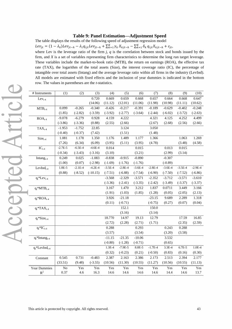
This article is protected by copyright. All rights reserved. 43
Table 9: Panel Estimation—Adjustment Speed The table displays the results of the following speed of adjustment regression model
𝐿𝑒𝑣𝑗𝑡 = (1 − 𝜆0)𝐿𝑒𝑣𝑗𝑡−ℎ − 𝜆1𝑞𝑖𝑗𝑡𝐿𝑒𝑣𝑗𝑡−ℎ + ∑ 𝛾𝑘𝐾𝑘=1 𝑋𝑘𝑗𝑡−ℎ − ∑ 𝛿𝑘
𝐾𝑘=1 𝑞𝑖𝑗𝑡𝑋𝑘𝑗𝑡−ℎ + 휀𝑗𝑡,
where Lev is the leverage ratio of the firm j, q is the correlation between stock and bonds issued by the
firm, and X is a set of variables representing firm characteristics to determine the long run target leverage.
These variables include the market-to-book ratio (MTB), the return on earnings (ROA), the effective tax
rate (TAX), the logarithm of the total assets (Size), the interest coverage ratio (IC), the percentage of
intangible over total assets (Intang) and the average leverage ratio within all firms in the industry (LevInd).
All models are estimated with fixed effects and the inclusion of year dummies is indicated in the bottom
row. The values in parentheses are the t-statistics.
# Instruments (1) (2) (3) (4) (5) (6) (7) (8) (9) (10)
Levt-4 0.720 0.669 0.659 0.668 0.657 0.664 0.668 0.647
(14.06) (11.12) (12.01) (11.06) (11.98) (10.98) (11.11) (10.62)
MTBt-4 0.099 -0.265 -0.340 -0.426 -0.217 -0.391 -0.189 -0.629 -0.402 -0.248
(1.85) (-2.82) (-3.59) (-3.92) (-2.77) (-3.64) (-2.44) (-6.02) (-3.72) (-2.63)
ROAt-4 -9.078 -6.279 0.928 4.159 4.222 4.321 4.125 4.252 4.499
(-3.86) (-3.36) (0.88) (2.55) (2.66) (2.67) (2.68) (2.56) (2.66)
TAXt-4 -1.953 -1.752 22.85 3.124 3.050
(-0.40) (-0.37) (7.42) (1.51) (1.48)
Sizet-4 1.081 1.178 1.350 1.176 1.489 1.177 1.366 1.063 1.269
(7.26) (6.34) (6.09) (3.95) (5.11) (3.95) (4.78) (3.48) (4.58)
ICt-4 -2.7E-5 -6.5E-4 -4.6E-4 0.014 0.015 0.013 0.015
(-0.34) (-3.43) (-3.16) (3.10) (3.21) (2.99) (3.14)
Intangt-4 0.249 0.025 -1.083 -0.838 -0.915 -0.890 -0.307
(1.00) (0.07) (-2.98) (-1.69) (-1.76) (-1.76) (-0.89)
LevIndt-4 1.8E-5 -2.1E-4 -4.2E-4 -3.5E-4 -2.8E-4 -3.6E-4 -2.8E-4 -3.6E-4 -3.5E-4 -2.9E-4
(0.88) (-8.52) (-10.15) (-7.51) (-6.88) (-7.54) (-6.90) (-7.50) (-7.52) (-6.86)
qt*Levt-4 -3.568 -2.329 -3.571 -2.352 -3.712 -3.571 -3.610
(-3.36) (-2.41) (-3.35) (-2.42) (-3.49) (-3.37) (-3.37)
qt*MTBt-4 3.167 1.470 3.212 1.837 0.0711 3.449 3.166
(1.91) (1.03) (1.85) (1.28) (0.05) (2.05) (2.13)
qt*ROAt-4 3.926 -21.18 -23.15 9.689 2.289 1.318
(0.11) (-0.71) (-0.75) (0.27) (0.07) (0.04)
qt*TAXt-4 152.1 150.0
(3.16) (3.14)
qt*Sizet-4 18.770 14.97 19.13 12.79 17.59 16.85
(2.72) (2.28) (2.71) (1.71) (2.35) (2.59)
qt*ICt-4 0.288 0.293 0.243 0.288
(3.57) (3.54) (3.20) (3.58)
qt*Intangt-4 -11.15 -21.35 -10.06 3.532
(-0.80) (-1.28) (-0.71) (0.65)
qt*LevIndt-4 1.3E-4 -7.9E-5 8.8E-5 -1.7E-4 3.3E-4 6.7E-5 1.0E-4
(0.32) (-0.23) (0.21) (-0.50) (0.83) (0.16) (0.30)
Constant 0.545 0.731 -0.483 2.387 2.163 2.386 2.173 2.513 2.394 2.177
(33.51) (9.48) (-3.55) (10.56) (11.30) (10.55) (11.27) (10.56) (10.55) (11.13)
Year Dummies No Yes Yes Yes Yes Yes Yes Yes Yes Yes
R2 0.37 4.6 16.3 14.6 14.6 14.6 14.6 14.4 14.6 13.7
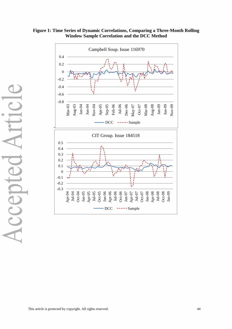
This article is protected by copyright. All rights reserved. 44
Figure 1: Time Series of Dynamic Correlations, Comparing a Three-Month Rolling
Window Sample Correlation and the DCC Method
-
-0.8
-0.6
-0.4
-0.2
0
0.2
0.4
Mar
-03
Au
g-0
3
Jan
-04
Jun
-04
No
v-0
4
Ap
r-0
5
Sep
-05
Feb
-06
Jul-
06
Dec
-06
May
-07
Oct
-07
Mar
-08
Au
g-0
8
Jan
-09
Jun
-09
No
v-0
9
Campbell Soup. Issue 116970
DCC Sample
-0.3
-0.2
-0.1
0
0.1
0.2
0.3
0.4
0.5
Ap
r-0
4
Jul-
04
Oct
-04
Jan
-05
Ap
r-0
5
Jul-
05
Oct
-05
Jan
-06
Ap
r-0
6
Jul-
06
Oct
-06
Jan
-07
Ap
r-0
7
Jul-
07
Oct
-07
Jan
-08
Ap
r-0
8
Jul-
08
Oct
-08
Jan
-09
CIT Group. Issue 184518
DCC Sample

This article is protected by copyright. All rights reserved. 45
Figure 2: Time Series of the Standard DCC Estimation and the Correspondent
Estimation Adjusted for Non-Trading Days (DCCD)
0
0.05
0.1
0.15
0.2
0.25
Jul-
02
Dec
-02
May
-03
Oct
-03
Mar
-04
Au
g-0
4
Jan
-05
Jun
-05
No
v-0
5
Ap
r-0
6
Sep
-06
Feb
-07
Jul-
07
Dec
-07
May
-08
Oct
-08
Mar
-09
Au
g-0
9
Ford Motor Credit. Issue 101077
Mean gap between prices: 1.45 days (mínimum)
DCC DCCD
-0.15
-0.1
-0.05
0
0.05
Mar
-03
May
-03
Jul-
03
Sep
-03
No
v-0
3
Jan
-04
Mar
-04
May
-04
Jul-
04
Sep
-04
No
v-0
4
Jan
-05
Mar
-05
May
-05
Jul-
05
Sep
-05
No
v-0
5
Jan
-06
CVS Corporation. Issue 126124
Mean gap between prices: 2.89 days (maximum)
DCC DCCD
-0.06
-0.04
-0.02
0
0.02
0.04
Oct
-04
Dec
-04
Feb
-05
Ap
r-0
5
Jun
-05
Au
g-0
5
Oct
-05
Dec
-05
Feb
-06
Ap
r-0
6
Jun
-06
Au
g-0
6
Oct
-06
Dec
-06
Feb
-07
Ap
r-0
7
Jun
-07
Au
g-0
7
Oct
-07
Dec
-07
Ford Motor Credit. Issue 67234. δ=53,04
Mean gap between prices: 1.83 days
DCC DCCD