evapotranspiration of tropical peat swamp forests
TRANSCRIPT

Instructions for use
Title Evapotranspiration of tropical peat swamp forests
Author(s) Hirano, Takashi; Kusin, Kitso; Limin, Suwido; Osaki, Mitsuru
Citation Global Change Biology, 21(5), 1914-1927https://doi.org/10.1111/gcb.12653
Issue Date 2015-05
Doc URL http://hdl.handle.net/2115/65234
RightsThis is the peer reviewed version of the following article: [Global Change Biology 2015 May;21(5):1914-1927], whichhas been published in final form at [10.1111/gcb.12653]. This article may be used for non-commercial purposes inaccordance with Wiley Terms and Conditions for Self-Archiving.
Type article (author version)
File Information Final MS_GCB15-1.pdf
Hokkaido University Collection of Scholarly and Academic Papers : HUSCAP
Title: Evapotranspiration of tropical peat swamp forests 1
Running title: Evapotranspiration of tropical PSFs 2
3
Takashi Hirano*, Kitso Kusin**, Suwido Limin* and Mitsuru Osaki* 4
*Research Faculty of Agriculture, Hokkaido University, Sapporo 060-8589, Japan 5
**CIMTROP, University of Palangkaraya, Palangkaraya 73112, Indonesia 6
7
Correspondence: Takashi Hirano, tel/fax +81-11-706-3689, e-mail: 8
10
Keywords: disturbances, drainage, eddy covariance, energy balance, ENSO, fire, groundwater 11
level, smoke, Southeast Asia 12
13
Abstract 14
In Southeast Asia, peatland is widely distributed and has accumulated a massive amount of 15
soil carbon, coexisting with peat swamp forest (PSF). The peatland, however, has been 16
rapidly degraded by deforestation, fires and drainage for the last two decades. Such 17
disturbances change hydrological conditions, typically groundwater level (GWL), and 18
accelerate oxidative peat decomposition. Evapotranspiration (ET) is a major determinant of 19
GWL, whereas information on the ET of PSF is limited. Therefore, we measured ET using the 20
eddy covariance technique for four to six years between 2002 and 2009, including El Niño 21
and La Niña events, at three sites in Central Kalimantan, Indonesia. The sites were different in 22
disturbance degree: a PSF with little drainage (UF), a heavily drained PSF (DF) and a drained 23
burnt ex-PSF (DB); GWL was significantly lowered at DF, especially in the dry season. The 24
ET showed a clear seasonal variation with a peak in the mid-dry season and a large decrease 25
in the late dry season, mainly following seasonal variation in net radiation (Rn). The Rn 26
drastically decreased with dense smoke from peat fires in the late dry season. Annual ET 27
forced to close energy balance for four years was 1636 53, 1553 117 and 1374 75 mm 28
yr-1
(mean 1 standard deviation), respectively, at UF, DF and DB. The undrained PSF (UF) 29
had high and rather stable annual ET, independently of El Niño and La Niña events, in 30
comparison with other tropical rainforests. The minimum monthly-mean GWL explained 80% 31
of interannual variation in ET for the forest sites (UF and DF); the positive relationship 32
between ET and GWL indicates that drainage by a canal decreased ET at DF through lowering 33
GWL. In addition, ET was decreased by 16% at DB in comparison with UF chiefly because of 34
vegetation loss through fires. 35
36
Introduction 37
In Southeast Asia, mainly Indonesia and Malaysia, peatland is widely distributed, coexisting 38
with swamp forest, over an area of 2.48 105 km
2 and accumulating up to 68.5 Pg of soil 39
organic carbon, which accounts for 11-14% of global peat carbon (Page et al., 2011). These 40
peatlands, however, have been rapidly devastated by deforestation and drainage for logging 41
and land-use change, with such disturbances often causing frequent large-scale peat fires 42
(Miettinen et al., 2012b; Page et al., 2002). As a result, the proportion of forest cover in the 43
peatlands of Peninsular Malaysia, Sumatra and Borneo fell from 77% to 36% from 1990 to 44
2010 (Miettinen et al., 2012b). In these regions, 20% of peatlands had been also converted to 45
plantations of oil palm and Acacia by 2010 (Miettinen et al., 2012a). These human pressures 46
have increased the vulnerability of the huge peat carbon pool and increased the risk for the 47
pool to be a large carbon source to the atmosphere chiefly because of peat fires and lowered 48
groundwater level (GWL) which stimulates the rate of biological oxidation (e.g. Hirano et al., 49
2012; Page et al., 2002). 50
The carbon balance of peatland is chiefly controlled by local hydrology (e.g. Bozkurt et 51
al., 2001; Limpens et al., 2008), which determines the water regime of surface peat. Under 52
unsaturation conditions, peat is aerated, and its soil organic compounds are easily oxidized 53
into carbon dioxide (CO2). Therefore, theoretically, drainage to lower GWL enhances 54
oxidative peat decomposition and its resultant CO2 emissions. Field studies have illustrated 55
such relationship with GWL from studies of peat subsidence (Couwenberg et al., 2009; 56
Hooijer et al., 2010; Hooijer et al., 2012) and soil CO2 efflux (Hirano et al., 2014; Jauhiainen 57
et al., 2012; Sundari et al., 2012) in tropical peatlands. Also, Hirano et al. (2012) showed that 58
the CO2 balance of tropical peat ecosystems was clearly related to GWL on both monthly and 59
annual bases. 60
The GWL results from water balance. Because tropical peatland is typically 61
ombrotrophic (Dommain et al., 2011; Page et al., 2004), GWL varies according to residuals 62
(storage change) between precipitation as input and evapotranspiration (ET) and discharge as 63
output. Although precipitation can be also affected by large-scale deforestation (Spracklen et 64
al., 2012), ET and runoff are directly affected by deforestation, fires and drainage, 65
respectively (e.g. Bosch & Hewlett, 1982; Dore et al., 2010; Sun et al., 2001). For example, 66
conversion from tropical forest to pasture decreased ET in Amazonia, especially in the dry 67
season (von Randow et al., 2004). To predict GWL under human pressures and thereby assess 68
the carbon balance of tropical peatland, it is crucial to quantify ET and elucidate the effects of 69
disturbances on ET. In addition, tropical forest plays an important role in hydrologic and 70
atmospheric circulations, which drive climate systems, both on regional and global scales by 71
massive ET and its resultant strong evaporative cooling (Bonan, 2008). Although peat swamp 72
forest in Malaysia and Indonesia except Papua (7.00 104 km
2, Miettinen et al., 2012b) 73
accounts for only 5% of the forest area in the two countries (1.29 106 km
2, Harris et al., 74
2012) in 2000, it is important to investigate the energy balance of tropical peat swamp forest 75
for better understanding of the ecosystem function of tropical forest, because its ground water 76
condition is different from that of other upland forest. Information on the energy balance and 77
ET of tropical peatland is still quite limited (Hirano et al., 2005). 78
We measured fluxes of sensible heat (H) and latent heat (lE) using the eddy covariance 79
technique and determined ET and energy balance at three sites within 15 km of each other on 80
tropical peatland near Palangkaraya, Central Kalimantan, Indonesia (Hirano et al., 2012). The 81
sites were different in disturbance degree: a peat swamp forest (PSF) with little drainage (UF), 82
a heavily drained PSF (DF) and a drained burnt ex-PSF with limited vegetation (DB). Here 83
we show the results of field measurement for four to six years between 2002 and 2009, 84
including El Niño and La Niña events and discuss seasonal and interannual variations in the 85
ET of PSF and the effects of anthropogenic disturbances due to drainage and fires on the ET. 86
Materials and Methods 87
Study site 88
The study was conducted in tropical peatlands near Palangkaraya, Central Kalimantan 89
province, Indonesia. A large peatland area was deforested and drained in this province during 90
the late 1990s according to a national project: the Mega Rice Project. Although the project 91
was terminated in 1999, it left vast degraded peatland. Three sites were located on flat terrain 92
within 15 km (Hirano et al., 2012): a PSF with little drainage (UF; 2.32S, 113.90E), a 93
drained PSF (DF; 2.35S, 114.14E) and a drained burnt ex-PSF with re-growing vegetation 94
(DB; 2.34S, 114.04E), which was dominated by fern plants. The DF and DB have been 95
drained by a large canal (25 m wide 3.5-4.5 m deep) excavated in 1996 and 1997. 96
Information of each site was detailed by our previous paper (Hirano et al., 2012). 97
98
Flux measurement 99
Eddy fluxes of sensible heat (H) and latent heat (lE) were measured on towers since July 2004 100
at a height of 36.5 m, November 2001 at 41.3 m and April 2004 at 3.0 m, respectively, at UF, 101
DF and DB using the eddy covariance technique with a sonic anemometer-thermometer 102
(CSAT3; Campbell Scientific Inc., USA) and an open-path CO2/H2O analyzer (LI7500; 103
Li-Cor Inc., USA) (Hirano et al., 2012). Sensor signals were recorded using a datalogger 104
(8421; Hioki E. E. Corp., Japan) at 10 Hz. Net radiation (Rn) and albedo were measured with 105
a radiometer (CNR-1; Kipp & Zonen, the Netherlands) at a height of 36.3, 40.6 and 3.3 m, 106
respectively, at UF, DF and DB. Air temperature and relative humidity were measured with a 107
platinum resistance thermometer and a capacitive hygrometer (HMP45; Vaisala, Finland) 108
installed in a non-ventilated radiation shield (DTR503A; Vaisala) at a height of 36.3, 41.7 and 109
1.5 m, respectively, at UF, DF and DB. Precipitation was measured with a tipping-bucket rain 110
gauge (TE525; Campbell Scientific Inc.) at a height of 41.0 m at DF. Sensor signals were 111
measured every 30 s; their half-hourly means were recorded using a datalogger (CR10X; 112
Campbell Scientific Inc.). Groundwater level (GWL), which was shown as a distance between 113
the ground (reference) and groundwater surfaces, was measured every 30 min with a water 114
level logger (DL/N; Sensor Technik Sirnach AG, Sienach, Switzerland or DCX-22 VG; Keller 115
AG, Winterthur, Switzerland) within 5 m from towers at the three sites. 116
117
Flux calculation 118
Half-hourly mean H and lE were calculated according to the following procedures: 1) removal 119
of noise spikes (Vickers & Mahrt, 1997), 2) planar fit rotation (Wilczak et al., 2001), 3) water 120
vapor correction for H (Hignett, 1992), 4) correction for high- and low-frequency losses using 121
a theoretical transfer function (Massman, 2000, Massman, 2001), 5) covariance calculation 122
using a block average and 6) density fluctuation correction for lE (Webb et al., 1980). 123
The sensitivity of an open-path analyzer (LI7500) for water vapor density was 124
calibrated by comparing half-hourly mean water vapor densities from the LI7500 and a 125
slow-response thermometer/hygrometer (HMP45) (Iwata et al., 2012), because the sensitivity 126
directly affects the covariance of water vapor density and vertical wind velocity. The 127
sensitivity was calculated every day as the slope of correlation between two water vapor 128
densities (y: LI7500, x: HMP45) using a moving window of 31 days, and then the daily 129
variation of the slope was smoothed by fitting a tenth-order spline curve. If correlation was 130
not significant (p > 0.05), the slope data were excluded from the fitting. Before the correlation 131
analysis, data were excluded in the rain and in the nighttime to avoid outliers due to raindrops 132
or dew condensation on the LI7500’s window. In addition to such data screening, data were 133
only used under the neutral condition of atmospheric stability for DB, because the LI7500 134
was installed 1.5 m higher than the HMP45. The reciprocal of the daily slope was applied as a 135
correction coefficient for the covariance. 136
We used flux data from July 2004 to August 2008, December 2001 to July 2008 and 137
April 2004 to September 2009, respectively, for UF, DF and DB. To calculate annual sums, 138
we defined the annual period of 365 or 366 days starting on July 10 or 11 (DOY192) and 139
ending on July 9 or 10 (DOY191) (Hirano et al., 2012). The whole rainy season was captured 140
in each annual period, because the rainy season usually starts in October and lasts until June 141
in this area (Hirano et al., 2012). In the period, annual sums were calculated for the four year 142
periods of 2004–2008, the six year periods of 2002–2008 and the five year periods of 2004–143
2009, respectively, for UF, DF and DB. 144
145
Quality control and gap filling of flux data 146
We first excluded flux data obtained during rain and when the mean wind direction was 147
within ±30°, ±35° and ±20° from the north, respectively, for UF, DF and DB, thereby 148
avoiding flow distortion caused by the tower. The azimuth angles were determined from 149
tower dimensions. Next, we calculated the difference between covariances determined from 150
the whole interval of 30 min and six intervals of 5 min. Flux data were excluded, if 151
covariance difference was larger than 250% (Foken & Wichura, 1996). Consequently, the 152
survival rates of H and lE data available for annual summations were 49% and 51%, 50% and 153
50%, and 46% and 64%, respectively, for UF, DF and DB. Data gaps were filled by the 154
look-up table (LUT) method using Rn and vapor pressure deficit (VPD) as predictors on a 155
half-hourly basis. The Rn and VPD were grouped into ten and three classes, respectively. The 156
LUT was created every three months: November–January, February–April, May–July and 157
August–October, considering climate conditions (Hirano et al., 2007). After gap filling, to 158
correct annual ET for the energy imbalance (Table S1), H and lE were forced to balance with 159
Rn (adjustment) using a ratio of H and lE (Bowen ratio) on a daily basis (Twine et al., 2000). 160
161
Calculation of bulk parameters 162
Bulk parameters of surface conductance (Gs) (Monteith, 1965), decoupling factor (Ω) (Jarvis 163
& McNaughton, 1986) and Priestley-Taylor coefficient (α) (Priestley & Taylor, 1972) were 164
calculated to interpret the seasonal variation and environmental response of ET. To avoid 165
instability and divergence, the bulk parameters around midday from 1000 to 1400 in no-rain 166
conditions were only used to calculate monthly means for the analysis (Ryu et al., 2008). Also, 167
albedo for shortwave radiation was calculated for the midday period when global radiation 168
was larger than 700 W m-2
(Hirano et al., 2007). 169
The Gs (m s-1
) stands for the integration of individual leaf’s stomatal conductance for 170
transpiration and surface wetness for evaporation, which was calculated backward from the 171
Penman-Monteith equation by replacing Rn – G with H + lE, because G was unavailable (Eqn. 172
1). This substitution would overestimate Gs because of energy imbalance (Table S1). 173
1
𝐺𝑠=
1
𝐺𝑎[𝜀(𝐻+𝑙𝐸)+𝜌𝐶𝑝𝐺𝑎
𝑉𝑃𝐷
𝛾
𝑙𝐸− 𝜀 − 1] (1) 174
where Ga is bulk aerodynamic conductance (m s-1
), ε is s/γ, s is the slope of relationship 175
between saturation vapor pressure and temperature (kPa K-1
), γ is psychrometric constant (= 176
0.067 kPa K-1
), ρ is air density (kg m-3
), Cp is specific heat of air at constant pressure (= 1007 177
J kg-1
K-1
), VPD is vapor pressure deficit (kPa). The Ga was calculated using the following 178
equation (Humphreys et al., 2006). 179
𝐺𝑎 = [2
𝜅𝑢∗(𝑑ℎ
𝑑𝑣)
2
3+
𝑢
𝑢∗2]
−1
(2) 180
where κ is von Karman constant (=0.4), u* is friction velocity (m s-1
), dh is thermal diffusivity, 181
dv is molecular diffusivity of water vapor and u is mean wind velocity (m s-1
). The ratio of dh 182
and dv (dh/dv) was set at 0.89 (Humphreys et al., 2006). 183
The Ω is an index (0 to 1) of decoupling between vegetation and the atmosphere for ET, 184
which was defined as follows: 185

Ω =𝜀+1
𝜀+1+𝐺𝑎𝐺𝑠
(3) 186
The Ω approaches 0 when ET is controlled by Gs and VPD (coupling), and approaches one 187
when ET is controlled by available energy (decoupling). 188
The α is the ratio of measured lE and equilibrium lE (lEeq), which is the lE of an 189
extended wet surface (Priestley & Taylor, 1972). The α was calculated using the following 190
equation (Flint & Childs, 1991). 191
α =𝑙𝐸
𝑙𝐸𝑒𝑞=
𝑙𝐸(𝑅𝑛−𝐺)𝑠
𝑠+𝛾
≅𝑙𝐸
(𝐻+𝑙𝐸)𝑠
𝑠+𝛾
=𝑠+𝛾
(1+𝛽)𝑠 (4) 192
where β is Bowen ratio. 193
194
Results 195
Seasonal variation 196
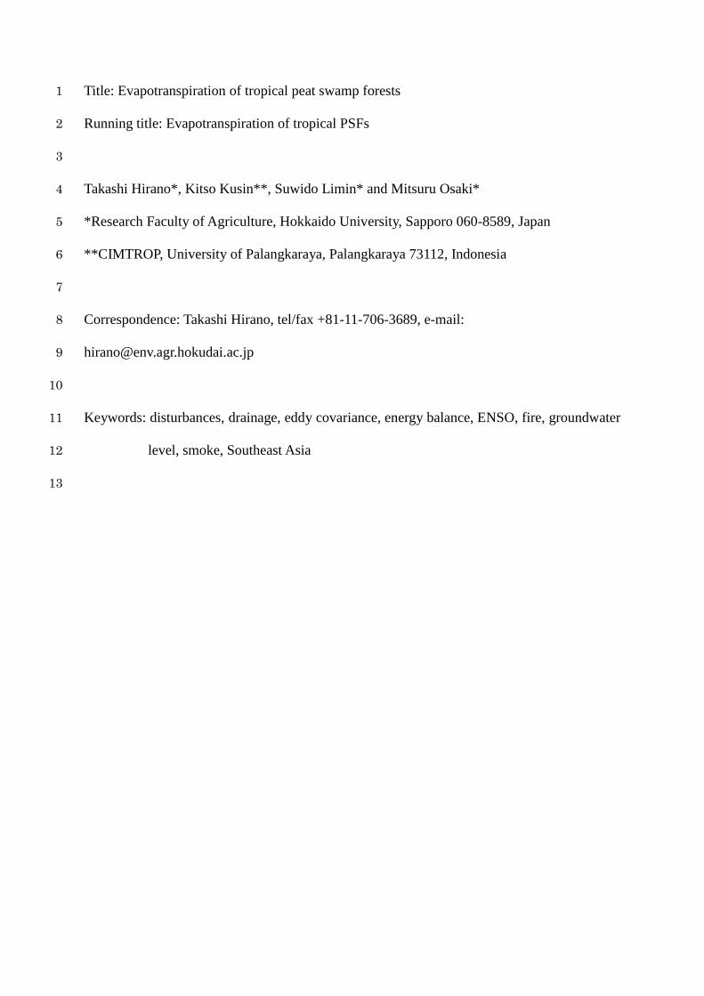
Monthly values of environmental elements, energy fluxes and bulk parameters are shown in 197
time sequence in Fig. 1. Precipitation shows seasonality with fluctuations due to El Niño and 198
La Niña events. According to sea surface temperature (SST) anomaly in the Niño 3.4 region, 199
El Niño and La Niña events occurred in the 02-03, 04-05 and 06-07 periods and the 05-06, 200
07-08 and 08-09 periods, respectively (NOAA, 201
http://www.cpc.ncep.noaa.gov/products/analysis_monitoring/ensostuff/ensoyears.stml). 202
Following the precipitation variation, GWL and VPD varied seasonally. In 2004 and 2005, the 203
less-vegetated ground surface at DB was studded with open water, which lowered albedo. A 204
large increase in albedo in 2006, especially at DB, was due to strong surface desiccation 205
caused by El Niño drought (Hirano et al., 2007). A massive amount of smoke emitted from 206
large-scale peat fires, which often occurs during El Niño drought, led to sudden reduction in 207
Rn in 2002 and 2006 (Hirano et al., 2007; Hirano et al., 2012; Hirano et al., 2005). 208
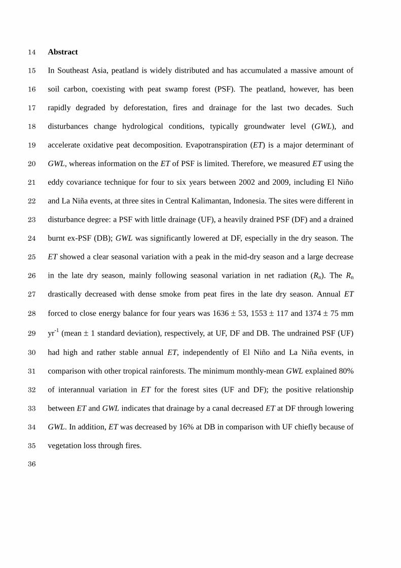
To clarify seasonal variation, monthly values were ensemble averaged for each site for 209
the common period of four years from August 2004 through July 2008 (Fig. 2). In addition, 210
monthly values were averaged for the rainy and dry seasons, respectively (Table 1); the 211
threshold to separate the two seasons was monthly precipitation of 100 mm (e.g. Malhi et al., 212
2002). As a result, 10 months out of a total (48 months) were classified as the dry season. On 213
average for the four years, August and September were in the dry season, and July with 214
monthly precipitation of 102 mm was the transition between the two seasons (Fig. 2). The 215
GWL reached its minimum of -0.55, -1.05 and -0.52 m at UF, DF and DB, respectively, in 216
October and was significantly lower in the dry season than in the rainy season. Midday VPD 217
began to increase in April and peaked in September at UF (1.84 kPa) and DF (1.92 kPa) and 218
in October at DB (2.28 kPa); it was significantly higher in the dry season. Albedo showed 219
seasonality similar to that of VPD with a peak in October at UF and DF and in November at 220
DB, which differed significantly between the two seasons except for DB. The Rn showed an 221
opposite peak in October because of shading due to dense smoke in 2006 (Fig. 1). However, 222
seasonal difference in Rn was not significant, because Rn is usually larger in the dry season if 223
no fires occur. Smoke from peat fires is critical for the radiation environment in the dry 224
season (Hirano et al., 2012). The H increased significantly in the dry season at DB, whereas 225
its seasonality was obscure at UF and DF. The lE or ET increased gradually from April 226
through August and decreased during September and October; the decrease would correspond 227
to Rn decrease. Seasonal difference in lE was significant only at UF. Similarly with H, Bowen 228
ratio increased significantly in the dry season only at DB. The ratio of lE and Rn increased 229
significantly in the dry season at UF and DF, except for DB. The Gs began to decrease in July 230
and reached an opposite peak in October at UF and DF and in November at DB, which 231
resembles GWL or the mirror image of midday VPD in seasonal variation, whereas significant 232
seasonal difference was detected only at DF, at which seasonal variation in GWL was the 233
largest. The Ω continued to decrease from July through October and showed significant 234
differences between the two seasons at the all sites. Although α showed a decreasing tendency 235
from July through October at DB, no significant seasonal variation was detected at all the 236
sites. 237
238
Interannual variation 239
Annual values of environmental elements, energy fluxes and bulk parameters are listed in 240
Table 2. Annual precipitation was 2446 50 mm yr-1
(mean 1 SD) on average for four 241
annual periods from the 04-05 through 07-08 periods; its interannual variation was small with 242
a coefficient of variance (CV) of 2.1%. Thus, the PSF is categorized into “tropical rainforest” 243
or “humid tropical forest” by the definition of annual precipitation > 1500 mm yr-1
and dry 244
season length < 6 months (Lewis, 2006). Annual dry period length (DPL), which is defined as 245
the number of days with 30-day moving total of precipitation less than 100 mm (Kume et al., 246
2011), averaged out at 90 33 days yr-1
with a CV of 34.2% for the same period. For the 247
seven years from the 02-03 period, annual precipitation was 2445 90 mm yr-1
(CV: 3.8%). 248
On the other hand, seven-year mean annual precipitation was calculated at 2411 393 mm 249
yr-1
(CV: 16.3%), if precipitation was summed following the solar calendar from 1 January 250
2002. Although the two means of annual precipitation were very similar each other 251
independently of summation periods, their SD values differed by a factor of 4.4. The annual 252
period starting on DOY 191, which can include almost the whole of one continuous rainy 253
season (Fig. 2), had much smaller interannual variation in precipitation than the solar calendar 254
period, because total precipitation in the rainy season was independent of its duration in 255
Indonesia (Hamada et al., 2002). This comparison reveals that annual precipitation depends 256
on its summation period. 257
The annual precipitation was rather stable, whereas DPL increased in the 02-03 and 258
6-07 periods because of the prolonged dry season due to El Niño drought. Following the 259
interannaul variation in the precipitation pattern, GWL, midday VPD and Rn showed 260
significant interannual difference (Table 3), whereas Rn was strongly affected by smoke from 261
peat fires. Also, there was significant interannual difference both in adjusted and unadjusted 262
ET to close energy balance, although their CVs were relatively small (<7.5%). Adjusted ET 263
was the highest in the 07-08 period (La Niña) and the lowest in the 06-07 period (El Niño), 264
which corresponds to the order of annual Rn. Among bulk parameters, only Ω differed 265
significantly. 266
267
Environmental response of ET 268
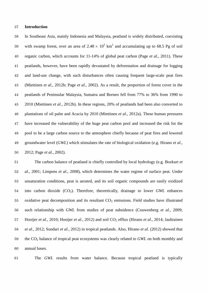
The relationship of ET with environmental elements was analysed using daily values of lE 269
and H under the condition that the gap ratio of half-hourly lE or H was lower than 20% for the 270
daytime from 600 through 1800 (Fig. 3). Both lE and H showed a significant linear 271
relationship, respectively, with Rn at the all sites. At DB, however, lE and H were apart from 272
the lines downward and upward, respectively, in the dry season in 2004 (Fig. 1), when 273
vegetation was still sparse and surface soil was desiccated. The lE / Rn averaged out at 0.84, 274
0.75 and 0.68, respectively, at UF, DF and DB. The lE showed a significant quadratic 275
relationship with GWL, which is a principal hydrological variable with a large annual 276
amplitude. The r2 value was the largest at DF with the largest GWL range. The lE normalized 277
by Rn (lE / Rn) showed a weak negative liner relationship with GWL at the all sites. On the 278
other hand, there was no relationship between lE / Rn and midday VPD (data not shown), 279
which is related to evaporative demand. 280
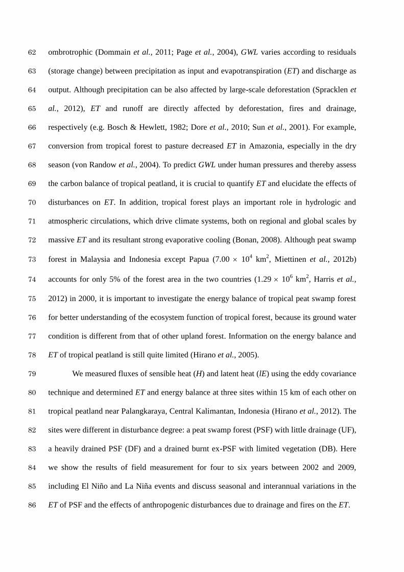
Adjusted annual ET showed a significant positive linearity (p < 0.01) with the minimum 281
monthly-mean GWL at each site with r2 vales of 0.98, 0.85 and 0.97, respectively, at UF, DF 282
and DB (data not shown). The r2 values were much larger than against annual mean GWL. 283
The strong linearity suggests that the minimum monthly-mean GWL drawdown by 10 cm 284
decreases annual ET by 19, 33 and 26 mm, respectively, at UF, DF and DB. Moreover, as a 285
whole, adjusted annual ET at the two forest sites showed a significant combined correlation 286
(r2 = 0.80, p < 0.01) (Fig. 4). Therefore, we can say that the minimum monthly-mean GWL is 287
a robust total predictor of annual ET of PSF, because the minimum GWL determines not only 288
the water regime in the dry season but also peat fire occurrence (Takahashi & Limin, 2011), 289
which drastically affects the radiation environment (Fig. 1). 290
For a further analysis, bulk parameters of Gs were plotted against GWL (Fig. 5). Data 291
were classified into three groups according to VPD, and quadratic curves were fitted to all 292
data groups, because many tree species decrease stomatal conductance in flooding (e.g. 293
Kozlowski, 1997). Significant convex curves (p < 0.05), except for a high VPD group at DB, 294
show that Gs didn’t decrease simply as GWL decreased. At UF, the curves suggest that Gs 295
peaked at GWLs of -0.10, -0.14 and -0.13 m, respectively, for VPD of <1.4, 1.4-1.9 and >1.9 296
kPa. Although Gs was lower at higher VPD, it was almost identical independently of VPD in 297
flooding conditions at DB, suggesting weak stomatal control on Gs. It was reported that some 298
flooding-tolerant trees acclimated to flooding and stomatal conductance recovered within a 299
flooding period (Herrera, 2013). At UF, however, there was no significant difference in Gs 300
(16.8 6.2 vs. 16.5 6.9 mm s-1
(mean 1 SD)) under the flooding condition (GWL > 0.0 m) 301
between the early (until February) and late (after March) rainy seasons. To compare the 302
response of Gs to GWL variation, data of the three sites were plotted together under the high 303
VPD condition (> 1.9 kPa) (Fig. 5d). The Gs began to decrease when GWL lowered below a 304
threshold at each site. The GWL threshold for Gs decrease was the lowest at DF, followed by 305
UF and DB in order. 306
307
Inter-site comparison 308
Seasonal means and annual values were compared among the three sites (Tables 1 to 3). The 309
GWL, which was measured as a distance between the ground and groundwater surfaces, was 310
significantly lower at DF because of drainage, whereas GWL at DB was very close to that of 311
UF in spite of the fact that DB was drained at the same time as DF. The relatively high GWL 312
at DB was chiefly caused by large ground subsidence due to peat fires (Hirano et al., 2014). 313
The Rn was significantly smaller at DB only in the rainy season probably because of 314
scattering open water surfaces. Midday VPD was significantly higher at DB chiefly owing to 315
lower lE and higher air temperature (data not shown). Albedo was significantly lower at DB 316
than UF only in the rainy season. The H was significantly larger at DB both in the rainy and 317
dry seasons. 318
Mean annual ET before adjustment to the energy balance for the four annual periods 319
was 1529 65, 1365 68 and 1197 52 mm yr-1
(mean 1 SD), respectively, for UF, DF 320
and DB. Uncertainties shown as one SD in annual ET due to random errors, which were 321
assessed according to our previous study (Hirano et al., 2012), were estimated to be 16 3, 17 322
2 and 10 1 mm yr-1
, respectively, for UF, DF and DB. The annual ET was the largest at UF, 323
followed by DF and DB in order, whereas lE showed no significant difference between DF 324
and DB in the dry season. After the adjustment, annual ET increased to 1636 53, 1553 117 325
and 1374 75 mm yr-1
, respectively, for UF, DF and DB; ET was significantly smaller at DB 326
than at UF and DF. As a result, Bowen ratio was the highest at DB both in the rainy and dry 327
seasons; it was significantly higher at DF than UF only in the rainy season. The Gs was the 328
highest at UF, followed by DF and DB in order, whereas no significant difference was found 329
between DF and DB in the dry season. The Ω was significantly higher at UF only in the rainy 330
season. The α was significantly lower at DB. 331
332
Discussion 333
Comparison of annual ET between PSF and other tropical forests 334
Unadjusted and adjusted annual ETs of an almost undrained PSF (UF) were 1529 65 and 335
1636 53 mm yr-1
, respectively, which accounted for 63% and 67% of annual precipitation 336
(P: 2446 50 mm yr-1
), respectively. The CV was 3.2% and 2.0%, respectively, for adjusted 337
ET and precipitation. Although the interannual variation of ET shown as CV was larger than 338
that of precipitation, it was smaller than those of tropical rainforests in Malaysian Borneo 339
(5.6%, Kume et al., 2011) and Peninsular Malaysia (4.0%, Kosugi et al., 2011). The annual 340
ET of UF was more than those of upland tropical rainforests in Malaysian Borneo (estimated 341
ET using a big-leaf model: 1323 74 mm yr-1
, P: 2600 272 mm yr-1
, ET / P: 0.51; Kume et 342
al., 2011), Peninsular Malaysia (adjusted ET: 1287 52 mm yr-1
, P: 1865 288 mm yr-1
, ET / 343
P: 0.69; Kosugi et al., 2011), central Amazonia (unadjusted ET: 1123 mm yr-1
, P: 2089 mm 344
yr-1
, ET / P: 0.54; Malhi et al., 2002), central Amazonia (unadjusted ET: 1123 9 mm yr-1
, P: 345
2091 215 mm yr-1
, ET / P: 0.54; Hutyra et al., 2007) and southwest China (adjusted ET: 346
1029 29 mm yr-1
, P: 1322 78 mm yr-1
, ET / P: 0.78; Li et al., 2010), a floodplain forest in 347
Amazonia (adjusted ET: 1332 21 mm yr-1
, P: 1692 181 mm yr-1
, ET / P: 0.79; Borma et 348
al., 2009), a wet montane cloud forest in Hawaii (adjusted ET: 1232 mm yr-1
, P: 2401 mm yr-1
, 349
ET / P: 0.51; Giambelluca et al., 2009) and the average of tropical forests in Asia and Oceania 350
regions (20S-20N) (ET: 1255 329 mm yr-1
, P: 2577 1057 mm yr-1
, ET / P: 0.49 (n = 57); 351
Komatsu et al., 2012), whereas it was less than that of a wet tropical forest in Costa Rica 352
(estimated ET using the Priestley-Taylor model: 2139 176 mm yr-1
, P: 3732 281 mm yr-1
, 353
ET / P: 0.57; Loescher et al., 2005). Although the evaporative fraction to precipitation (ET / 354
P) was lower in UF than in tropical rainforests in Peninsular Malaysia (0.69) and southwest 355
China (0.78) and an Amazonian floodplain forest (0.79), the PSF with high GWL is ranked 356
high among moist tropical forests with annual precipitation more than 2000 mm yr-1
(Kume et 357
al., 2011). In comparison with a tropical rainforest in Malaysian Borneo (Kume et al., 2011), 358
the PSF at UF had 13% more Rn and 52% higher VPD (0.76 kPa) on an annual basis. This 359
higher evaporative demand is a potential reason of the higher ET of the PSF, together with 360
high GWL. 361
362
Environmental response of ET 363
The ET was chiefly controlled by Rn at all the sites, because the relationship between ET and 364
GWL or VPD was weak. The Rn determined the temporal variation of lE by 54, 65 and 59% 365
(r2), respectively, at UF, DF and DB on a daily basis (Fig. 3). Evaporative fractions (lE / Rn) 366
were on average 0.84, 0.75 and 0.68, respectively, at UF, DF and DB. Fisher et al. (2009) 367
showed a positive relationship between lE and Rn with high r2 of 0.87 and an evaporative 368
fraction of 0.72 from a synthesis analysis of 21 pan-tropical eddy covariance sites. We can say 369
that the PSF at UF with a higher evaporative fraction has a high evaporative ability among 370
tropical ecosystems. As a result, the PSF showed a low Bowen ratio of 0.19 in comparison 371
with an average (0.30) of the 21 tropical sites (Fisher et al., 2009). 372
The lE showed relatively clear seasonal variation (Fig. 2); lE continued to increase from 373
the late rainy season to the mid-dry season and decreased in the late-dry season. The annual 374
amplitudes of the seasonal variation in lE were 2.6, 2.2 and 2.7 MJ m-2
day-1
on a monthly 375
basis, respectively, at UF, DF and DB, which were equivalent to ETs of 1.07, 0.92 and 1.10 376
mm day-1
, respectively. A similar ET increase in the dry season was also reported for tropical 377
forests in Amazonia (da Rocha et al., 2004; Hasler & Avissar, 2007; Hutyra et al., 2007) and 378
Thailand (Tanaka et al., 2008), which was attributed to increased Rn and the lack of drought 379
stress due to deep root systems. The lE decrease in the late dry season was enhanced during El 380
Niño drought in 2002 and 2006, when peat fires occurred and consequently Rn decreased 381
sharply (Fig. 1). However, lE / Rn increased conversely even during the peat fires, except for 382
at DB in 2004. These facts indicate that the lE decrease in the late dry season was chiefly 383
caused by Rn decrease due to smoke or haze and evaporative efficiency on Rn didn’t decrease 384
even in such drought conditions. As a result, lE / Rn remained high during the late rainy 385
season and the dry season (Fig. 2). On the other hand, Gs continued to decrease during the dry 386
season probably because of stomatal closure due to water stress by GWL decrease and VPD 387
increase (Fig. 5). The decreases from July to October or November were 5.3, 6.5 and 4.3 mm 388
s-1
, respectively, at UF, DF and DB. Thus, relatively stable lE / Rn during the dry season was 389
probably attributed to the compensation of Gs decrease and VPD increase. Severe drought in 390
2006 decreased Gs remarkably (Fig. 1). Correspondingly, Ω largely decreased during the dry 391
season, especially at DB with sparse, low vegetation. Although many tree species decrease 392
stomatal conductance in flooding (e.g. Kozlowski, 1997), the effect of flooding on Gs was 393
limited (Fig. 5) and was not reflected on the seasonal variation of Gs (Fig. 2), because 394
enhanced evaporation from the flooded ground would compensate the decrease of 395
transpiration due to stomatal closure. 396
397
Effects of drainage and fires 398
The ET measurement started at DF about five years after the excavation of a large canal, 399
which has functioned as effective drainage. Thus, GWL was significantly lower at DF than at 400
UF (Table 3). The difference in GWL between the two forest sites was larger in the dry season 401
than in the rainy season; GWL difference was on average 0.37 m in February-April and 0.50 402
m in October (Fig. 2). As a result, the annual range of GWL was larger at DF (0.79 m) than at 403
UF (0.66 m). Especially in El Niño years, the GWL difference increased in the late dry season 404
(Fig. 1). The lowering of the minimum GWL decreased annual ET linearly (Fig. 4). However, 405
no significant difference in adjusted annual ET was found between DF and UF by paired t-test 406
(p = 0.085), although mean annual ET was 5% less at DF (Table 2). 407
Although Gs was significantly lower at DF than UF both in the rainy and dry seasons 408
(Table 1), a GWL threshold, at which Gs began to decrease, was much lower at DF than at UF 409
(Fig. 5d), suggesting the adaptation of tree species at DF to the low GWL environment during 410
more than five years after canal excavation. There is a report that 83% of root biomass of a 411
PSF in the same area as UF was distributed in the surface soil layer of 0-0.25 m in depth and 412
remaining 17% was in the underlying layer of 0.25-0.50 m (Sulistiyanto, 2004). Roots of PSF 413
trees are concentrated in the surface peat level in comparison with deeply-rooted upland 414
tropical forests (e.g. Davidson et al., 2011; Nesptad et al., 1994). Tree roots probably 415
penetrated deeper into seasonally unsaturated soil following GWL lowering. Annual 416
evaporative fraction (lE / Rn) increased linearly (r2 = 0.88) for six years from the 02-03 to 417
07-08 periods at DF. In addition, Gs at DF was averaged in a drought condition (GWL: -1.4 to 418
-1.2 m, VPD: 2.0 to 2.5 kPa) for each of three El Niño events in 2002, 2004 and 2006; the 419
means were 6.3 2.5, 8.5 3.9 and 7.8 2.8 mm s-1
, respectively, for 2002, 2004 and 2006. 420
As a result, mean Gs in 2002 was significantly lower than those in 2004 and 2006 (Tukey’s 421
HSD, p < 0.05). These facts support the hypothesis of adaptation. The Gs and ET most 422
probably decreased by GWL lowering due to drainage at DF, because Gs was significantly 423
lower in the dry season only at DF (Table 1) and annual ET showed a positive correlation with 424
the minimum GWL (Fig. 4). However, the drainage effect would be eased gradually because 425
of the adaptation through root redistribution. 426
The DB, a burnt site with regrowing vegetation, was drained together with DF by a canal 427
running between the two sites, whereas GWL at DB was very close to that at UF, because the 428
ground subsided largely owing to peat fires (Hirano et al., 2014). Adjusted annual ET of 1374 429
75 mm yr-1
, which accounted for 56% of annual precipitation, was significantly lower than 430
those of the other two forest sites because of low tree density; the annual ET was equivalent to 431
84% and 88% of UF and DF, respectively (Tables 2 and 3). However, the annual ET was 432
compatible with that of a tropical rainforest in Malaysian Borneo (Kume et al., 2011). 433
Conversely, annual H was significantly higher than those at UF and DF, and consequently 434
Bowen ratio was significantly higher. Generally, albedo is higher in unforested areas with 435
short vegetation than in forest (e.g. Bonan, 2008), which can result in lower Rn in unforested 436
areas. In Amazonia, land conversion from forest to pasture increased albedo by 55% and 437
decreased Rn by 13% (von Randow et al., 2004). Midday albedo at a pasture and an upland 438
rice field in Amazonia were reported to be 0.15-0.17 (Sakai et al., 2004). At DB, however, 439
annual mean midday albedo was 0.087 0.007 and showed no significant difference with the 440
forest sites. Also, annual Rn showed no significant difference, whereas it was smaller by 6% 441
than that at UF. The unexpected lower albedo at DB was attributable to dark color of burnt 442
peat and scattered open water. On the other hand, annual mean Gs was less than 50% of that at 443
UF (Table 2) chiefly owing to low leaf area index. Although Gs showed no significant 444
difference between the rainy and dry seasons (Table 1), inter-site difference between DB and 445
UF increased by 50% in the dry season. The Gs responded to GWL lowering more sensitively 446
than those of UF and DF (Fig. 5); Gs began to decrease at about -0.1 m. This sensitive 447
response could be due to the shallow rooting depth (von Randow et al., 2012) of the 448
regrowing vegetation, which was dominated by fern and sedge plants (Hirano et al., 2012). 449
Tree loss due to fires and subsequent vegetation succession decreased Gs and consequently ET, 450
whereas the decrease in ET was less than expected by Gs decrease, because albedo didn’t 451
decrease, midday VPD increased and GWL remained high owing to large subsidence (Fig. 2). 452
Annual discharge can be calculated from precipitation and ET to be 810 53, 893 105 453
and 1072 71 mm yr-1
, respectively, at UF, DF and DB, on the assumption that storage 454
change is negligible on an annual basis. Although no significant difference was found 455
between UF and DF, annual discharge tended to increase by drainage and significantly 456
increased by tree loss due to fires. A negative linear relationship was found between inter-site 457
difference in annual discharge (DF minus UF) and the minimum monthly GWL at DF (p < 458
0.05) (data not shown). The increase of discharge potentially increases fluvial organic carbon 459
outflow (Moore et al., 2013). Our results indicate that disturbances due to drainage and fires 460
decreased ET and increased discharge; the effect of drainage was remarkable in El Niño years 461
with lower GWL. This study can contribute to a better assessment of the water balance of PSF 462
by providing reliable information on ET to hydrological models and improve our knowledge 463
of the carbon dynamics of PSF through a better prediction of GWL which is determined as a 464
result of water balance. 465
466

Acknowledgements 467
This work was supported by JSPS Core University Program, JSPS KAKENHI (Nos. 468
13375011, 15255001, 18403001, 21255001 and 25257401) and the JST-JICA Project 469
(SATREPS) (Wild Fire and Carbon Management in Peat-Forest in Indonesia). 470
471
References 472
Bonan G (2008) Forests and climate change: forcings, feedbacks, and the climate benefits of 473
forests. Science, 320, 1444-1449. 474
Borma LS, da Rocha H. R., Cabral OM et al. (2009) Atmosphere and hydrological controls of 475
the evapotranspiration over a floodplain forest in the Bananal Island region, Amazonia. 476
Journal of Geophysical Research, 114, G01003, doi:10.1029/2007JG000641. 477
Bosch J, Hewlett J (1982) A review of catchment experiments to determine the effect of 478
vegetation changes on water yield and evapotranspiration. Journal of Hydrology, 55, 479
3-23. 480
Bozkurt S, Lucisano M, Moreno L, Neretnieks I (2001) Peat as a potential analogue for the 481
long-term evolution in landfills. Earth-Science Reviews, 53, 95-147. 482
Couwenberg J, Dommain R, Joosten H (2009) Greenhouse gas fluxes from tropical peatlands 483
in south-east Asia. Global Change Biology, 16, 1715-1732. 484
da Rocha HR, Goulden ML, Miller SD, Menton MC, Pinto LDVO, de Freitas HC, Figueira 485
AMES (2004) Seasonality of waer and heat fluxes over a tropical forest in eastern 486
Amazonia. Ecological Applications, 14, S22-S32. 487
Davidson E, Lefebvre PA, Brando PM et al. (2011) Carbon inputs and water uptake in deep 488
soils of an eastern Amazon forest. Forest Science, 57, 51-58. 489
Dommain R, Couwenberg J, Joosten H (2011) Development and carbon sequestration of 490
tropical peat domes in south-east Asia: links to post-glacial sea-level changes and 491
Holocene climate variability. Quaternary Science Reviews, 30, 999-1010. 492
Dore S, Kolb TE, Montes-Helu M et al. (2010) Carbon and water fluxes from ponderosa pine 493
forests disturbed by wildfire and thinning. Ecological Applications, 20, 663-683. 494
Fisher JB, Malhi Y, Bonal D et al. (2009) The land-atmosphere water flux in the tropics. 495
Global Change Biology, 15, 2694-2714. 496
Flint AL, Childs SW (1991) Use of the Priestley-Taylor evaporation equation for soil water 497
limited conditions in a small forest clearcut. Agricultural and Forest Meteorology, 56, 498
247-260. 499
Foken T, Wichura B (1996) Tools for quality assessment of surface-based flux measurements. 500
Agricultural and Forest Meteorology, 78, 83-105. 501
Giambelluca T, Martin R, Asner G et al. (2009) Evapotranspiration and energy balance of 502
native wet montane cloud forest in Hawai‘i. Agricultural and Forest Meteorology, 149, 503
230-243. 504
Hamada J, Yamanaka MD, Matsumoto J, Fukao S, Winarso PA, Sribimawati T (2002) Spatial 505
and temporal variations of the rainy season over Indonesia and their link to ENSO. 506
Journal of the Meteorological Society of Japan, 80, 285-310. 507
Harris NL, Brown S, Hagen SC et al. (2012) Baseline map of carbon emissions from 508
deforestation in tropical regions. Science, 336, 1573-1576. 509
Hasler N, Avissar R (2007) What controls evapotranspiration in the Amazon basin? Journal of 510
Hydrometeorology, 8, 380-395. 511
Herrera A (2013) Responses to flooding of plant water relations and leaf gas exchange in 512
tropical tolerant trees of a black-water wetland. Frontiers in Plant Science, 4, 513
doi:10.3389/fpls.2013.00106. 514
Hignett P (1992) Corrections to temperature measurements with a sonic anemometer. 515
Boundary-Layer Meteorology, 61, 175-187. 516
Hirano T, Kusin K, Limin S, Osaki M (2014) Carbon dioxide emissions through oxidative 517
peat decomposition on a burnt tropical peatland. Global Chang Biology, 20, 555-565. 518
Hirano T, Segah H, Harada T, Limin S, June T, Hirata R, Osaki M (2007) Carbon dioxide 519
balance of a tropical peat swamp forest in Kalimantan, Indonesia. Global Change 520
Biology, 13, 412-425. 521
Hirano T, Segah H, Kusin K, Limin S, Takahashi H, Osaki M (2012) Effects of disturbances 522
on the carbon balance of tropical peat swamp forests. Global Change Biology, 18, 523
3410-3422. 524
Hirano T, Segah H, Limin S et al. (2005) Energy balance of a tropical peat swamp forest in 525
Central Kalimantan, Indonesia. Phyton-Annales Rei Botanicae, 45, 67-71. 526
Hooijer A, Page S, Canadell JG, Silvius M, Kwadijk J, Wosten H., Jauhiainen J. (2010) 527
Current and future CO2 emissions from drained peatlands in Southeast Asia. 528
Biogeosciences, 7, 1505-1514. 529
Hooijer A, Page S, Jauhiainen J, Lee WA, Lu XX, Idris A, Anshari G (2012) Subsidence and 530
carbon loss in drained tropical peatlands. Biogeosciences, 9, 1053-1071. 531
Humphreys ER, Lafleur PM, Flanagan LB, Hedstrom N, Syed KH, Glenn AJ, Granger R 532
(2006) Summer carbon dioxide and water vapor fluxes across a range of northern 533
peatlands. Journal of Geophysical Research, 111, G04011, 534
doi:10.1029/2005JG000111. 535
Hutyra LR, Munger JW, Saleska SR et al. (2007) Seasonal controls on the exchange of carbon 536
and water in an Amazonian rain forest. Journal of Geophysical Research, 112, G03008, 537
doi:10.1029/2006JG000365. 538
Iwata H, Harazono Y, Ueyama M (2012) Sensitivity and offset changes of a fast-response 539
open-path infrared gas analyzer duting long-term observations in an Arctic 540
environment. Journal of Agricultural Meteorology, 68, 175-181. 541
Jarvis PG, Mcnaughton KG (1986) Stomatal control of transpiration: scaling up from leaf to 542
region. Advances in Ecological Research, 15, 1-49. 543
Jauhiainen J, Hooijer A, Page SE (2012) Carbon dioxide emissions from an Acacia plantation 544
on peatland in Sumatra, Indonesia. Biogeosciences, 9, 617-630. 545
Komatsu H, Cho J, Matsumoto K, Otsuki K (2012) Simple modeling of the global variation in 546
annual forest evapotranspiration. Journal of Hydrology, 420-421, 380-390. 547
Kosugi Y, Takanashi S, Tani M et al. (2012) Effect of inter-annual climate variability on 548
evapotranspiration and canopy CO2 exchange of a tropical rainforest in Peninsular 549
Malaysia. Journal of Forest Research, 17, 227-240. 550
Kozlowski KK (1997) Responses of woody plants to flooding and salinity. Tree Physiology 551
Monograph, 1, 1-29. 552
Kume T, Tanaka N, Kuraji K et al. (2011) Ten-year evapotranspiration estimates in a Bornean 553
tropical rainforest. Agricultural and Forest Meteorology, 151, 1183-1192. 554
Lewis SL (2006) Tropical forests and the changing earth system. Philosophical Transactions 555
of The Royal Society, Biological Sciences, 361, 195-210. 556
Li Z, Zhang Y, Wang S, Yuan G, Yang Y, Cao M (2010) Evapotranspiration of a tropical rain 557
forest in Xishuangbanna, southwest China. Hydrological Processes, 24, 2405-2416. 558
Limpens J, Berendse F, Blodau C et al. (2008) Peatlands and the carbon cycle: from local 559
processes to global implications - a synthesis. Biogeosciences, 5, 1475-1491. 560
Loescher HW, Gholz HL, Jacobs JM, Oberbauer SF (2005) Energy dynamics and modeled 561
evapotranspiration from a wet tropical forest in Costa Rica. Journal of Hydrology, 315, 562
274-294. 563
Malhi Y, Pegoraro E, Nobre AD, Pereira MGP, Grace J, Culf AD, Clement R (2002) The 564
energy and water dynamics of a central Amazonian rain forest. Journal of Geophysical 565
Research, 107, 8061, doi:10.1029/2001JD000623 566
Massman WJ (2000) A simple method for estimating frequency response corrections for eddy 567
covariance systems. Agricultural and Forest Meteorology, 104, 185-198. 568
Massman WJ (2001) Reply to comment by Rannik on "A simple method for estimating 569
frequency response for eddy systems". Agricultural and Forest Meteorology, 107, 570
247-251. 571
Miettinen J, Hooijer A, Shi C et al. (2012a) Extent of industrial plantations on Southeast 572
Asian peatlands in 2010 with analysis of historical expansion and future projections. 573
GCB Bioenergy, 4, 908-918. 574
Miettinen J, Shi C, Liew SC (2012b) Two decades of destruction in Southeast Asia's peat 575
swamp forests. Frontiers in Ecology and the Environment, 10, 124-128. 576
Monteith JL (1965) Evaporation and the environment. Symposium of the Sciety of Exploratory 577
Biology, 19, 205-234. 578
Moore S, Evans CD, Page SE et al. (2013) Deep instability of deforested tropical peatlands 579
revealed by fluvial organic carbon fluxes. Nature, 493, 660-664. 580
Nesptad DC, de Carvalho CR, Davidson EA et al. (1994) The role of deep roots in the 581
hydrological and carbon cycles of Amazonian forests and pastures. Nature, 372, 582
666-669. 583
Page SE, Rieley JO, Banks CJ (2011) Global and regional importance of the tropical peatland 584
carbon pool. Global Change Biology, 17, 798-818. 585
Page SE, Siegert F, Rieley JO, Boehm HDV, Jaya A, Limin S (2002) The amount of carbon 586
released from peat and forest fires in Indonesia during 1997. Nature, 420, 61-65. 587
Page SE, Wűst RaJ, Weiss D, Rieley JO, Shotyk W, Limin SH (2004) A record of Late 588
Pleistocene and Holocene carbon accumulation and climate change from an equatorial 589
peat bog (Kalimantan, Indonesia): implications for past, present and future carbon 590
dynamics. Journal of Quaternary Science, 19, 625-635. 591
Priestley CHB, Taylor RJ (1972) On the assessment of surface heat flux and evaporation 592
using large-scale parameters. Monthly Weather Review, 100, 81-92. 593
Ryu Y, Baldocchi DD, Ma S, Hehn T (2008) Interannual variability of evapotranspiration and 594
energy exchange over an annual grassland in California. Journal of Geophysical 595
Research, 113, D09104, doi:10.1029/2007JD009263. 596
Sakai RK, Fitzjarrald DR, Moraes OLL et al. (2004) Land-use change effects on local energy, 597
water, and carbon balances in an Amazonian agricultural field. Global Change Biology, 598
10, 895-907. 599
Spracklen DV, Arnold SR, Taylor CM (2012) Observations of increased tropical rainfall 600
preceded by air passage over forests. Nature, 489, 282-285. 601
Sulistiyanto Y (2004) Nutrient dynamics in different sub-types of peat sawmp forest in 602
Central Kalimantan, Indonesia. Ph. D. thesis, The University of Nottingham, 387 pp. 603
Sun G, Mcnulty S, Shepard J et al. (2001) Effects of timber management on the hydrology of 604
wetland forests in the sourthern United States. Forest Ecology and Management, 143, 605
227. 606
Sundari S, Hirano T, Yamada H, Kusin K, Limin S (2012) Effects of groundwater level on soil 607
respiration in tropical peat swamp forests. Journal of Agricultural Meteorology, 68, 608
121-134. 609
Takahashi H, Limin SH (2011) Water in peat and peat fire in tropical peatland. In: Third 610
International Workshop on: Wild Fire and Carbon Management in Peat-forest in 611
Indonesia. (eds Osaki M, Takahashi H, Honma T et al.) pp. 49-54, Hokkaido 612
University and University of Palangkaraya. 613
Tanaka N, Kume T, Yoshifuji N et al., (2008) A review of evapotranspiration estimates from 614
tropical forests in Thailand and adjacent regions. Agricultural and Forest Meteorology, 615
148, 807-819. 616
Twine TE, Kustas WP, Norman JM et al. (2000) Correcting eddy-covariance flux 617
underestimates over a grassland. Agricultural and Forest Meteorology, 103, 279-300. 618
Vickers D, Mahrt L (1997) Quality control and flux sampling probelms for tower and aircraft 619
data. Journal of Atmospheric and Oceanic Technology, 14, 512-526. 620
von Randow C, Manzi AO, Kruijt B et al. (2004) Comparative measurements and seasonal 621
variations in energy and carbon exchange over forest and pasture in South West 622
Amazonia. Theoretical and Applied Climatology, 78, 5-26. 623
von Randow RCS, von Randow C, Hutjes RWA, Tomasella J, Kruijt B (2012) 624
Evapotranspiration of deforested areas in central and southwestern Amazonia. 625
Theoretical and Applied Climatology, 109, 205-220. 626
Webb EK, Pearman GI, Leuning R (1980) Correction of flux measurements for density effects 627
due to heat and water vapor transfer. Quarterly Journal of the Royal Meteorological 628
Society, 106, 85-106. 629
Wilczak JM, Oncley SP, Stage SA (2001) Sonic anemometer tilt correction algorithms. 630
Boundary-Layer Meteorology, 106, 85-106. 631
632

Supporting Information 633
Additional Supporting Information is available in the online version of this article: 634
Data S1. Supporting text describing energy imbalance, including references and summary 635
table (Table S1). 636
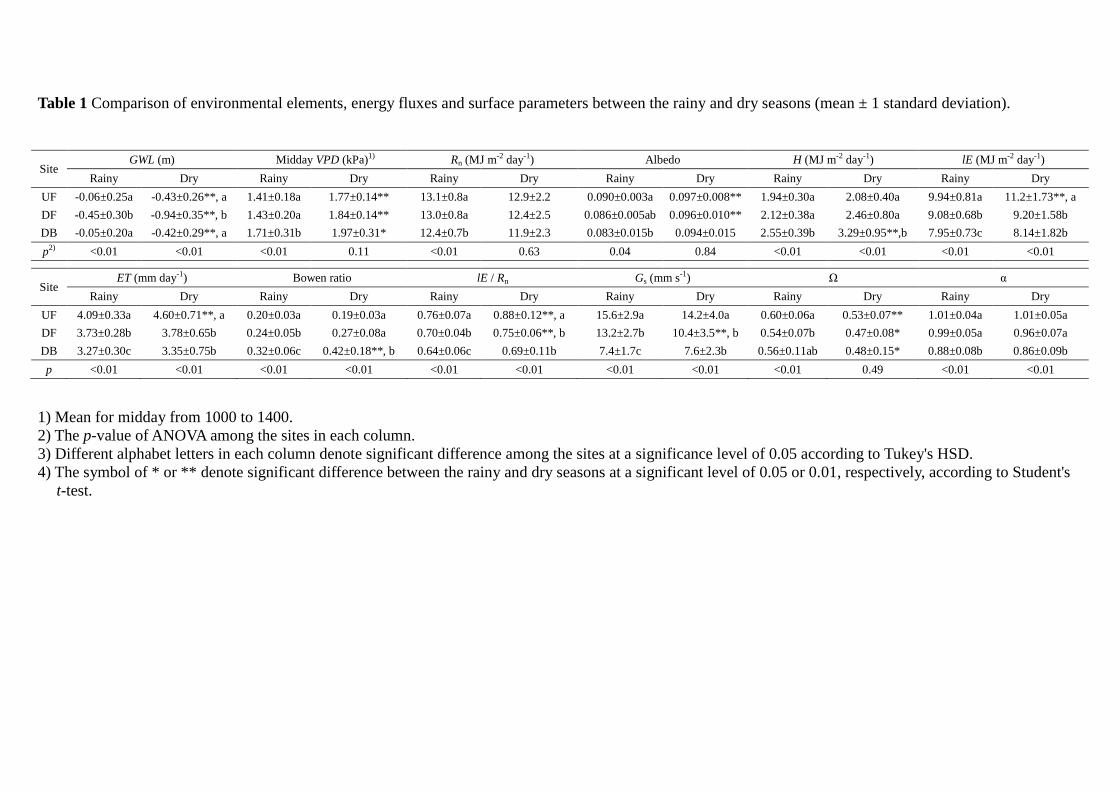
Table 1 Comparison of environmental elements, energy fluxes and surface parameters between the rainy and dry seasons (mean ± 1 standard deviation).
Site GWL (m) Midday VPD (kPa)1) Rn (MJ m-2 day-1) Albedo H (MJ m-2 day-1) lE (MJ m-2 day-1)
Rainy Dry Rainy Dry Rainy Dry Rainy Dry Rainy Dry Rainy Dry
UF -0.06±0.25a -0.43±0.26**, a 1.41±0.18a 1.77±0.14** 13.1±0.8a 12.9±2.2 0.090±0.003a 0.097±0.008** 1.94±0.30a 2.08±0.40a 9.94±0.81a 11.2±1.73**, a
DF -0.45±0.30b -0.94±0.35**, b 1.43±0.20a 1.84±0.14** 13.0±0.8a 12.4±2.5 0.086±0.005ab 0.096±0.010** 2.12±0.38a 2.46±0.80a 9.08±0.68b 9.20±1.58b
DB -0.05±0.20a -0.42±0.29**, a 1.71±0.31b 1.97±0.31* 12.4±0.7b 11.9±2.3 0.083±0.015b 0.094±0.015 2.55±0.39b 3.29±0.95**,b 7.95±0.73c 8.14±1.82b
p2) <0.01 <0.01 <0.01 0.11 <0.01 0.63 0.04 0.84 <0.01 <0.01 <0.01 <0.01
Site
ET (mm day-1) Bowen ratio lE / Rn Gs (mm s-1) Ω α
Rainy Dry Rainy Dry Rainy Dry Rainy Dry Rainy Dry Rainy Dry
UF 4.09±0.33a 4.60±0.71**, a 0.20±0.03a 0.19±0.03a 0.76±0.07a 0.88±0.12**, a 15.6±2.9a 14.2±4.0a 0.60±0.06a 0.53±0.07** 1.01±0.04a 1.01±0.05a
DF 3.73±0.28b 3.78±0.65b 0.24±0.05b 0.27±0.08a 0.70±0.04b 0.75±0.06**, b 13.2±2.7b 10.4±3.5**, b 0.54±0.07b 0.47±0.08* 0.99±0.05a 0.96±0.07a
DB 3.27±0.30c 3.35±0.75b 0.32±0.06c 0.42±0.18**, b 0.64±0.06c 0.69±0.11b 7.4±1.7c 7.6±2.3b 0.56±0.11ab 0.48±0.15* 0.88±0.08b 0.86±0.09b
p <0.01 <0.01 <0.01 <0.01 <0.01 <0.01 <0.01 <0.01 <0.01 0.49 <0.01 <0.01
1) Mean for midday from 1000 to 1400.
2) The p-value of ANOVA among the sites in each column.
3) Different alphabet letters in each column denote significant difference among the sites at a significance level of 0.05 according to Tukey's HSD.
4) The symbol of * or ** denote significant difference between the rainy and dry seasons at a significant level of 0.05 or 0.01, respectively, according to Student's
t-test.
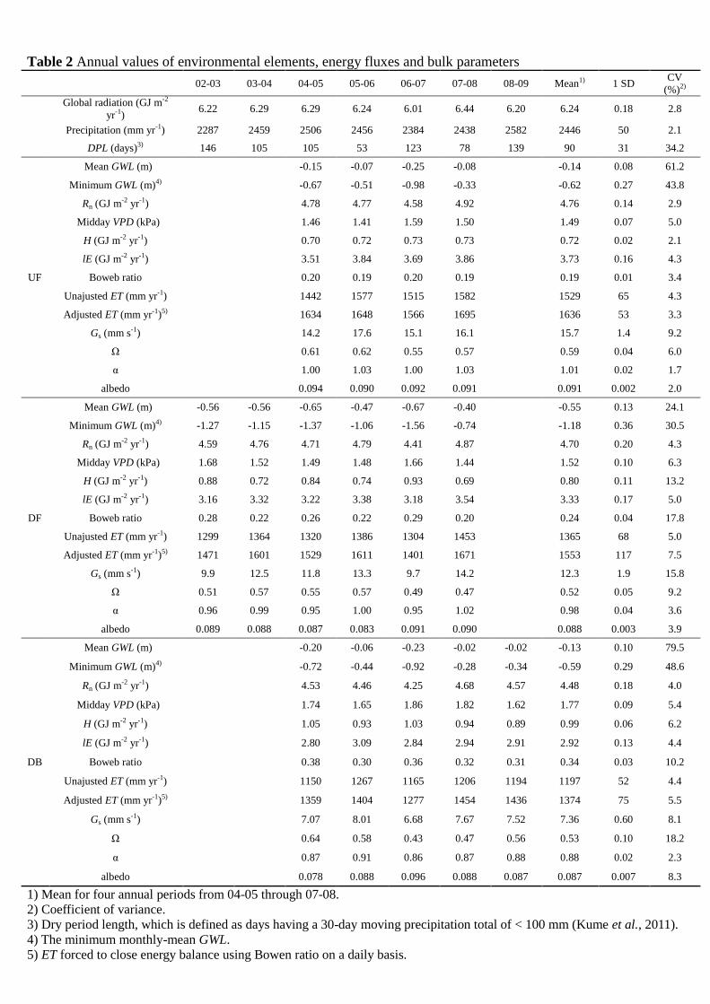
Table 2 Annual values of environmental elements, energy fluxes and bulk parameters
02-03 03-04 04-05 05-06 06-07 07-08 08-09 Mean1) 1 SD CV
(%)2)
Global radiation (GJ m-2
yr-1) 6.22 6.29 6.29 6.24 6.01 6.44 6.20 6.24 0.18 2.8
Precipitation (mm yr-1) 2287 2459 2506 2456 2384 2438 2582 2446 50 2.1
DPL (days)3) 146 105 105 53 123 78 139 90 31 34.2
UF
Mean GWL (m) -0.15 -0.07 -0.25 -0.08 -0.14 0.08 61.2
Minimum GWL (m)4)
-0.67 -0.51 -0.98 -0.33
-0.62 0.27 43.8
Rn (GJ m-2 yr-1)
4.78 4.77 4.58 4.92
4.76 0.14 2.9
Midday VPD (kPa)
1.46 1.41 1.59 1.50
1.49 0.07 5.0
H (GJ m-2 yr-1)
0.70 0.72 0.73 0.73
0.72 0.02 2.1
lE (GJ m-2 yr-1)
3.51 3.84 3.69 3.86
3.73 0.16 4.3
Boweb ratio
0.20 0.19 0.20 0.19
0.19 0.01 3.4
Unajusted ET (mm yr-1)
1442 1577 1515 1582
1529 65 4.3
Adjusted ET (mm yr-1)5)
1634 1648 1566 1695
1636 53 3.3
Gs (mm s-1)
14.2 17.6 15.1 16.1
15.7 1.4 9.2
Ω
0.61 0.62 0.55 0.57
0.59 0.04 6.0
α
1.00 1.03 1.00 1.03
1.01 0.02 1.7
albedo 0.094 0.090 0.092 0.091 0.091 0.002 2.0
DF
Mean GWL (m) -0.56 -0.56 -0.65 -0.47 -0.67 -0.40 -0.55 0.13 24.1
Minimum GWL (m)4) -1.27 -1.15 -1.37 -1.06 -1.56 -0.74
-1.18 0.36 30.5
Rn (GJ m-2 yr-1) 4.59 4.76 4.71 4.79 4.41 4.87
4.70 0.20 4.3
Midday VPD (kPa) 1.68 1.52 1.49 1.48 1.66 1.44
1.52 0.10 6.3
H (GJ m-2 yr-1) 0.88 0.72 0.84 0.74 0.93 0.69
0.80 0.11 13.2
lE (GJ m-2 yr-1) 3.16 3.32 3.22 3.38 3.18 3.54
3.33 0.17 5.0
Boweb ratio 0.28 0.22 0.26 0.22 0.29 0.20
0.24 0.04 17.8
Unajusted ET (mm yr-1) 1299 1364 1320 1386 1304 1453
1365 68 5.0
Adjusted ET (mm yr-1)5) 1471 1601 1529 1611 1401 1671
1553 117 7.5
Gs (mm s-1) 9.9 12.5 11.8 13.3 9.7 14.2
12.3 1.9 15.8
Ω 0.51 0.57 0.55 0.57 0.49 0.47
0.52 0.05 9.2
α 0.96 0.99 0.95 1.00 0.95 1.02
0.98 0.04 3.6
albedo 0.089 0.088 0.087 0.083 0.091 0.090
0.088 0.003 3.9
DB
Mean GWL (m) -0.20 -0.06 -0.23 -0.02 -0.02 -0.13 0.10 79.5
Minimum GWL (m)4)
-0.72 -0.44 -0.92 -0.28 -0.34 -0.59 0.29 48.6
Rn (GJ m-2 yr-1)
4.53 4.46 4.25 4.68 4.57 4.48 0.18 4.0
Midday VPD (kPa)
1.74 1.65 1.86 1.82 1.62 1.77 0.09 5.4
H (GJ m-2 yr-1)
1.05 0.93 1.03 0.94 0.89 0.99 0.06 6.2
lE (GJ m-2 yr-1)
2.80 3.09 2.84 2.94 2.91 2.92 0.13 4.4
Boweb ratio
0.38 0.30 0.36 0.32 0.31 0.34 0.03 10.2
Unajusted ET (mm yr-1)
1150 1267 1165 1206 1194 1197 52 4.4
Adjusted ET (mm yr-1)5)
1359 1404 1277 1454 1436 1374 75 5.5
Gs (mm s-1)
7.07 8.01 6.68 7.67 7.52 7.36 0.60 8.1
Ω
0.64 0.58 0.43 0.47 0.56 0.53 0.10 18.2
α
0.87 0.91 0.86 0.87 0.88 0.88 0.02 2.3
albedo 0.078 0.088 0.096 0.088 0.087 0.087 0.007 8.3
1) Mean for four annual periods from 04-05 through 07-08.
2) Coefficient of variance.
3) Dry period length, which is defined as days having a 30-day moving precipitation total of < 100 mm (Kume et al., 2011).
4) The minimum monthly-mean GWL.
5) ET forced to close energy balance using Bowen ratio on a daily basis.
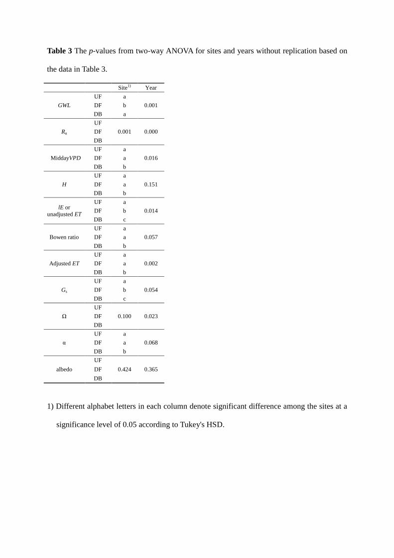
Table 3 The p-values from two-way ANOVA for sites and years without replication based on
the data in Table 3.
Site1) Year
GWL
UF a
0.001 DF b
DB a
Rn
UF
0.001 0.000 DF
DB
MiddayVPD
UF a
0.016 DF a
DB b
H
UF a
0.151 DF a
DB b
lE or
unadjusted ET
UF a
0.014 DF b
DB c
Bowen ratio
UF a
0.057 DF a
DB b
Adjusted ET
UF a
0.002 DF a
DB b
Gs
UF a
0.054 DF b
DB c
Ω
UF
0.100 0.023 DF
DB
α
UF a
0.068 DF a
DB b
albedo
UF
0.424 0.365 DF
DB
1) Different alphabet letters in each column denote significant difference among the sites at a
significance level of 0.05 according to Tukey's HSD.
Fig. 1. Time series of monthly values of environmental elements, energy fluxes and bulk
parameters at the three sites (UF, DF and DB) between 2001 and 2009. The 3-month
running mean of sea surface temperature anomalies in the Niño 3.4 region is shown (a).
El Niño and La Niña events are characterized by a five consecutive 3-month means with
thresholds above +0.5 and below -0.5C, respectively (NOAA,
http://www.cpc.ncep.noaa.gov/products/analysis_monitoring/ensostuff/ensoyears.stml).
GWL: groundwater level, midday VPD: vapor pressure deficit between 1000 and 1400,
Rn: net radiation, H: sensible heat flux, lE: latent heat flux, Gs: bulk surface conductance,
Ω: decoupling coefficient, α: Priestley-Taylor coefficient.
Fig. 2. Mean seasonal variations in monthly values of environmental elements, energy fluxes
and bulk parameters at the three sites (UF, DF and DB) from August 2004 to July 2008.
GWL: groundwater level, midday VPD: vapor pressure deficit between 1000 and 1400,
Rn: net radiation, H: sensible heat flux, lE: latent heat flux, Gs: bulk surface conductance,
Ω: decoupling coefficient, α: Priestley-Taylor coefficient.
Fig. 3. Relationships between energy fluxes and environmental elements at the three sites (UF,
DF and DB) on a daily basis. Lines (a, b, c, g, h and i) and quadratic curves (d, e and f)
were fitted (p < 0.05). Grey symbols at DB (c) were measurements in the dry season in
2004, which were excluded from the fitting. H: sensible heat flux, lE: latent heat flux,
Rn: net radiation, GWL: groundwater level.
Fig. 4. Combined relationship between annual evapotranspiration (ET) and the minimum
monthly- mean groundwater level (GWL) for UF and DF. A significant line was fitted
(p < 0.01).
Fig. 5. Relationships between bulk surface conductance (Gs) and groundwater level (GWL) at
UF (a), DF (b) and DB (c). Data were divided into three groups according to vapor
pressure deficit (VPD) and a quadratic curve was fitted to each group (p < 0.05). Data in
each VPD group were binned into deciles by GWL. The relationships are compared
among the three sites using the deciles in a high VPD condition (> 1.9 kPa) (d). Dark
grey symbols at DB (c) were measurements in the dry season in 2004, which were
excluded from the fitting.
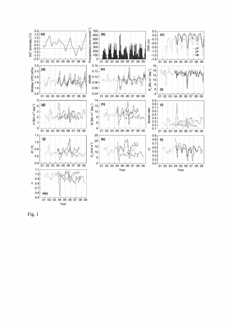
Fig. 1
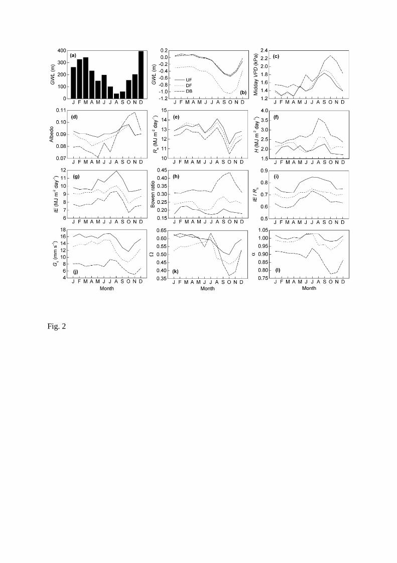
Fig. 2
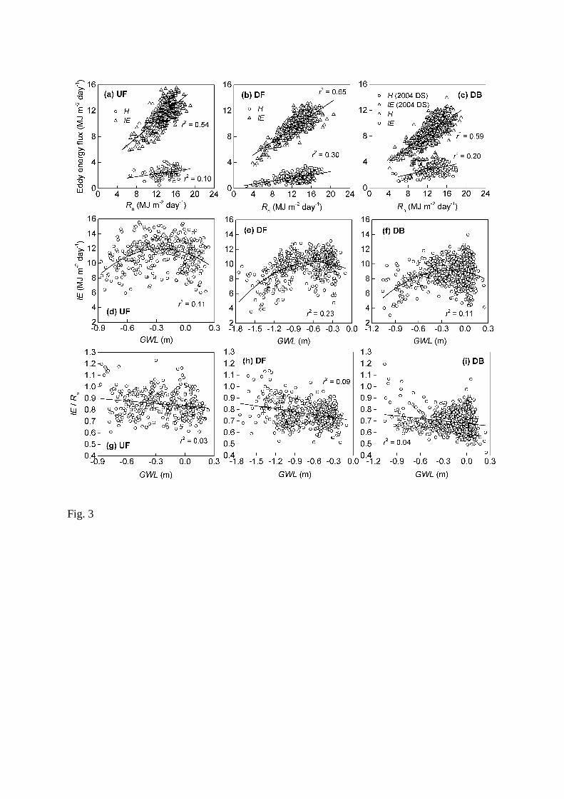
Fig. 3
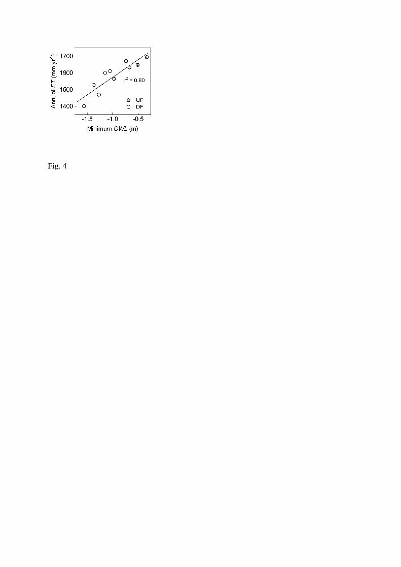
Fig. 4
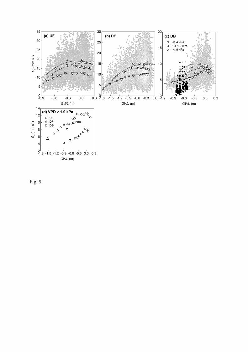
Fig. 5