evaluation of thermal diffusivity of soil · pdf fileevaluation of thermal diffusivity of soil...

467

EVALUATION OF THERMAL DIFFUSIVITY OF SOIL NEAR THE SURFACE: METHODS AND RESULTSB. EvstatiEvUniversity of Ruse, BG – 7017 Ruse, Bulgaria

Abstract

EvstatiEv, B., 2013. Evaluation of thermal diffusivity of soil near the surface: methods and results. Bulg. J. Agric. Sci., 19: 467-471

in the present study has been developed a method for evaluation of the mean daily thermal diffusivity of soil, assuming it is vertically inhomogeneous. the method uses data for the temperature variation of soil at three depths. additionally the soil surface heat flow has been defined as a function of the thermal conductivity and thermal diffusivity coefficients. The method’s performance conditions have been defined and their critical value has been determined for sensors with accuracy 0.1 °C. the method performance has been validated using data for the soil temperature variation at depths 1 cm, 10cm and 20 cm, acquired experimentally on the territory of the University of Ruse. the soil thermal diffusivity has been evaluated using the developed method and the harmonics method, considered to be the most reliable one. The results showed that the new method gives more accurate results than the harmonics one for days with low temperature amplitudes and for days with changing weather conditions.

Key words: soil temperature, thermal diffusivity, soil heat flow

Bulgarian Journal of Agricultural Science, 19 (No 3) 2013, 467-471Agricultural Academy

E-mail: [email protected]

Introduction

the thermal diffusivity is an important soil property, used in many areas as agriculture, climatology, engineering, etc. it greatly affects the soil temperature profile, which determines the earth’s heat and mass transfer, and is an important param-eter in energy balance applications such as land surface mod-eling, numerical weather forecasting and climate prediction (Holmes et al., 2008).

There are multiple known methods, used for evaluation of the soil thermal diffusivity. Two of the most common meth-ods are the amplitude and the phase ones, which present the soil temperature variation as a sine wave. However, the as-sumption that the soil temperature could be expressed as a single sine wave leads to significant errors under certain con-ditions. van Wijk (1963) suggested that this error could be reduced by using a multiple harmonic Fourier series to de-scribe more accurately the soil temperature fluctuation. This led to the introduction of the arctangent algorithm, presenting the soil temperature with two harmonics (Nerpin and Chud-novskii, 1967).

Horton et al. (1983) further developed the sine wave am-plitude and phase methods, considering higher harmonics,

by approximating the thermal diffusivity for a temperature variation expressed with two harmonics. More recently, Heu-sinkveld et al. (2004) presented a more accurate method, which expands the soil temperature variation in Fourier se-ries with multiple harmonics (harmonics method).

all of the above algorithms assume vertically homoge-nous soil; however, the thermal diffusivity can vary in depth. For this purpose Gao et al. (2003, 2008a) approximated the thermal diffusivity assuming it has a vertical gradient (con-duction-convection method). if the vertical gradient is 0, the method reduces to the common phase and amplitude ones.

it has been observed that many of these methods tend to return inaccurate data under certain environmental condi-tions (Horton et al., 1983). verhoef et al. (1996) examined the soil thermal diffusivity at the HaPEX-sahel site by using five algorithms. The conclusion was that the amplitude and the harmonic methods are the most reliable. another experi-mental comparison showed that the amplitude and the phase methods produce realistic estimates only for vertically ho-mogenous dry soils (Gao et al., 2008a). it has also been deter-mined that the water movement in soil is not negligible and can vary significantly in height (Gao et al., 2008a, b). Gao et al. (2009) also compared all of the above algorithms us-

B. Evstatiev468

ing experimentally acquired data. The results showed that the conduction-convection method returns more accurate results than the other methods excluding the harmonics one. the lat-ter returns the most reliable results in most cases with the exception of days with changing weather conditions.

a common problem for all of the above models is that they assume the soil temperature variation is a periodic function, which is a necessary condition to expand it in Fourier series. This requirement is met when the daily temperature variation of the soil surface is in a steady state condition. However, when rainy/cloudy ones follow sunny days, the assumption is incorrect and the accuracy of these methods decreases (Gao et al., 2009). another problem is most of the methods assume vertically homogenous soil, which is applicable only for very thin soil layers.

The goal of the study is to develop a new method for eval-uation of the mean daily thermal diffusivity of soil, assuming vertically inhomogeneous soils and applicable for both steady and unsteady states of the daily soil temperature variation.

Materials and Methods

Theoretical formulation and used dependenciesthe heat transfer in the classical theory in a one-dimen-

sional isotropic medium is described by:

∂∂

∂∂

=∂∂

tT

ttTC .. l (1)

where T is the soil temperature, 0C;t – the time, s;C – the volumetric heat capacity, J.m-3.K-1;λ – the soil thermal conductivity coefficient, W.m-1.K-1.in many cases, it can be assumed that a soil is vertically

homogenous, in which case C and λ are independent of depth, which allows to present equation (1) as:

tT

zTk

∂∂

=∂

∂2

2. (2)

where k is the soil thermal diffusivity coefficient, m2.s-1;z – the soil depth, m.in most cases, the investigated soil layer is inhomogeneous

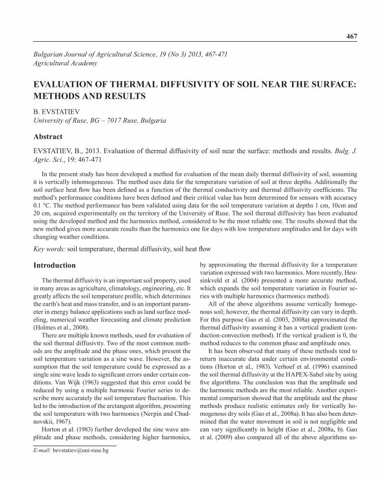
and anisotropic. If it is divided into two bordering homoge-nous layers with heights δ12=z2-z1 and δ32=z3-z2 (Figure 1), the heat transfer processes could be expressed as (asHRaE 2001):

323232

32

121212

1222 ....

. C

QCQ

tTT tZ

ttZ

, °C, (3)

where Q12 and Q32 are the heat flows, directed from z1 and z3 towards z2, W.m-2;

ρ12 and ρ32 – the densities of the two soil layers, kg.m-3; δ12 and δ32 – the heights of the two soil layers, m; C12 and C32 – the specific heat capacities of the two soil

layers, J.kg-1.K-1; ∆t - the time interval, s; Тz2

t and Тz2t+∆t - the soil temperatures at depth z2, in the

moments of time t and t+∆t respectively, 0C.the suggested method requires soil temperature measure-

ments at three depths: z1, z2 and z3 (fig. 1). This method re-lies on the approximation that the thermal diffusivity of soil between the depths z1 and z2 is equal to k1, and between the depths z2 and z3 – to k2. in order to determine the mean daily values of the two coefficients, it is assumed that k1 and k2 are constants during the investigated day.

The instantaneous values of the heat flows Q12 and Q32 are given with:

)32(12

2)3(1)32(12)32(12

ZZZ TTQ

, W.m-2, (4)

where λ12 and λ32 are the heat conductivities of the two soil layers, W.m-1.K-1.

Based on equations (3) and (4), the temperature variation of the soil at depth z2 can be evaluated with: ( ) ( )

232

232

12

2122

.2.1.

tZ

tZ

tZ

tZt

Ztt

ZTTkTTktTT , °C. (5)

The thermal diffusivities k1 and k2 of the two layers can be evaluated using the least square algorithm, by comparing the experimental and modeled values of the soil temperature at depth z2:

( ) min0

.2.2

MAXt

t

ttModZ

ttExpZ TT , (6)

where Тz2.Expt+∆t is the experimental value of the tempera-

ture at depth z2, and Тz2.Modt+∆t – the modeled one.

If the thermal conductivity coefficients λ12 and λ32 of the two layers are known, the heat flows Q12 and Q32 could be determined with: ( )

1.2 1212

232

232212 k

TTkt

TTQt

Zt

Zt

Ztt

Z

, W.m-2 (7)

and ( )

2.1 3232

212

212232 k

TTkt

TTQt

Zt

Zt

Ztt

Z

, W.m-2. (8)

in case the topmost sensor measures the surface tem-perature and the thermal conductivity λ12 of the top layer is known, the instantaneous value of the heat flow between the environment and the soil surface can be determined with: ( )

11.1 12

212

1211k

zTTkt

TTQ

tZ

tZ

tZ

ttZ

Env

, W.m-2. (9)

λ

Evaluation of Thermal Diffusivity of Soil near the Surface: Methods and Results 469

Performance conditionsthe method requires a couple of conditions to be met in

order to function properly. The first condition is to have posi-tive soil temperatures during the investigated period:

0)( >tTsoil ; Maxtt <<0 . (10)

This requirement is forced by the non-zero soil water con-tent, whose phase changes (melting and freezing) lead to a great energy consumption or discharge. since these process-es are not taken into account in the presented method, they would lead to inaccurate estimates of k1 and k2.

The second performance condition follows from equa-tion (2) - the thermal diffusivity can be obtained only for soil whose temperature varies in both time and depth:

CritTTGradTTGradCritCritTTGradTTGradCrit

ZZMinZZMax

ZZMinZZMax

2323

212121

,°C, (11)

where GradMax and GradMin are the maximal and minimal instantaneous temperature gradients of the soil layers (z1÷z2) and (z3÷z2), 0C;

Crit - the critical value of the criteria, for which the ther-mal diffusivity can be determined accurately, 0C.

the value Crit depends on the accuracy of the tempera-ture sensors and should be determined experimentally.

Results and Discussion

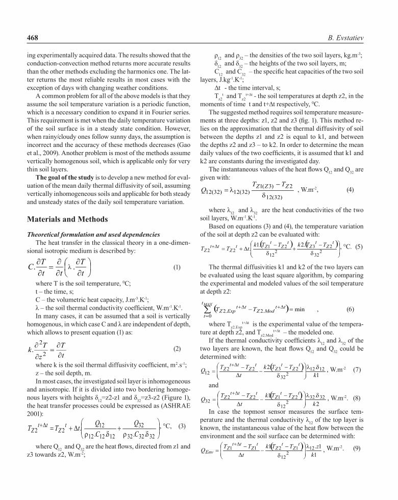
The experimental data used in this study were acquired at the territory of the University of Ruse. the soil temperatures were measured at three depths (1 cm, 10 cm and 20 cm), us-ing temperature sensors DS18B20 with accuracy 0.10C. the spacing between the sensors was fixed on a XPS fiber with

heat conductivity 0.03 W.m-1.K-1. The sensors were connected through a 1-Wire network to the USB port of a personal com-puter, where the measurements were read and stored in a da-tabase at a 10 minutes interval.

in this study have been presented and analyzed experimen-tal data for the period from 19.11.2011 to 30.04.2012. in accor-dance with the first performance condition of the method, only days with positive soil temperatures have been analyzed.

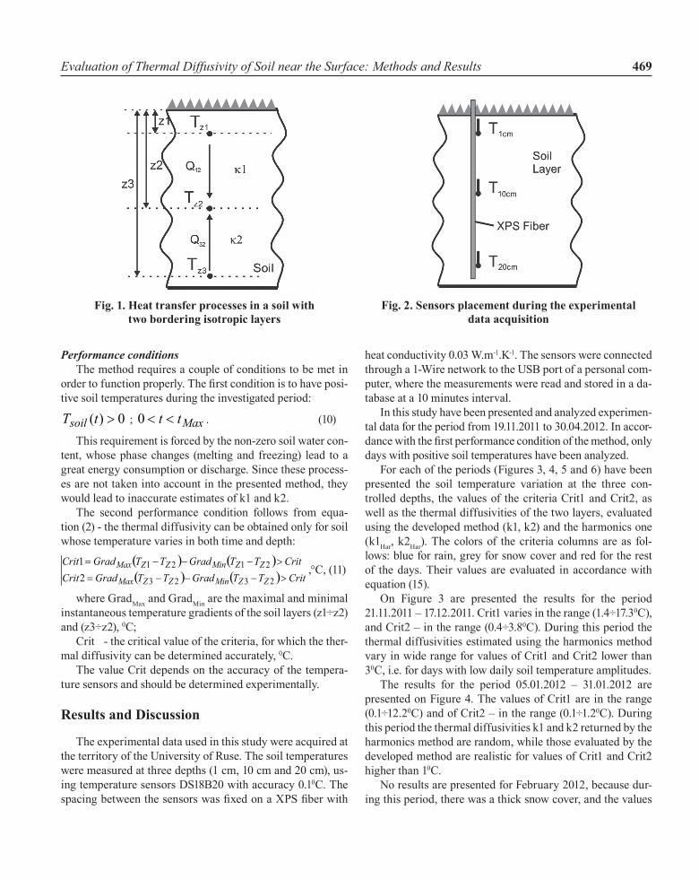
For each of the periods (Figures 3, 4, 5 and 6) have been presented the soil temperature variation at the three con-trolled depths, the values of the criteria Crit1 and Crit2, as well as the thermal diffusivities of the two layers, evaluated using the developed method (k1, k2) and the harmonics one (k1Har, k2Har). the colors of the criteria columns are as fol-lows: blue for rain, grey for snow cover and red for the rest of the days. Their values are evaluated in accordance with equation (15).

On Figure 3 are presented the results for the period 21.11.2011 – 17.12.2011. Crit1 varies in the range (1.4÷17.30C), and Crit2 – in the range (0.4÷3.80C). During this period the thermal diffusivities estimated using the harmonics method vary in wide range for values of Crit1 and Crit2 lower than 30C, i.e. for days with low daily soil temperature amplitudes.

the results for the period 05.01.2012 – 31.01.2012 are presented on Figure 4. the values of Crit1 are in the range (0.1÷12.20C) and of Crit2 – in the range (0.1÷1.20C). During this period the thermal diffusivities k1 and k2 returned by the harmonics method are random, while those evaluated by the developed method are realistic for values of Crit1 and Crit2 higher than 10C.

No results are presented for February 2012, because dur-ing this period, there was a thick snow cover, and the values

Fig. 1. Heat transfer processes in a soil with two bordering isotropic layers

Fig. 2. Sensors placement during the experimental data acquisition

B. Evstatiev470

0369

121518°C

T1cm

T10cm

T20cm

0246810

0

1

2

3

4

21/1

1/20

1122

/11/

2011

23/1

1/20

1124

/11/

2011

25/1

1/20

114/

12/2

011

5/12

/201

16/

12/2

011

7/12

/201

111

/12/

2011

12/1

2/20

1113

/12/

2011

14/1

2/20

1115

/12/

2011

16/1

2/20

1117

/12/

2011

m2/s x 10-7°C

Crit2

k2

k2 Har

012345

0369

121518 m2/s x 10-7°C

Crit1

k1

k1 Har

Fig. 3. Soil temperature variation and mean daily thermal diffusivities evaluated using the harmonics

method and the developed method in the period 21.11.2011 – 17.12.2011

0369

121518°C

T01cm

T10cm

T20cm

0246810

0.0

0.3

0.6

0.9

1.2

5/1/

2012

6/1/

2012

7/1/

2012

8/1/

2012

9/1/

2012

20/1

/201

221

/1/2

012

22/1

/201

223

/1/2

012

24/1

/201

225

/1/2

012

26/1

/201

227

/1/2

012

28/1

/201

229

/1/2

012

30/1

/201

231

/1/2

012

m2/s x 10-7 °C

Crit2

k2

k2 Har

0246810

02468

1012 m2/s x 10-7°C

Crit1

k1

k1 Har



010

20

30

40

50°CT01cm

T10cm

T20cm

0

1

2

05

101520253035°C

Crit1k1

k1 Har

0246810

0

2

4

6

12/0

3/20

1213

/03/

2012

14/0

3/20

1215

/03/

2012

16/0

3/20

1217

/03/

2012

18/0

3/20

1219

/03/

2012

20/0

3/20

1221

/03/

2012

22/0

3/20

1223

/03/

2012

24/0

3/20

1225

/03/

2012

26/0

3/20

1227

/03/

2012

28/0

3/20

1229

/03/

2012

30/0

3/20

1231

/03/

2012

m2/s x 10-7°C

Crit2

k2

k2 Har

m2/s x 10-7



0

1

2

34

08

16243240°C

Crit1

k1

k1 Har

1357911

0

2

4

6

01/0

4/20

1202

/04/

2012

03/0

4/20

1204

/04/

2012

05/0

4/20

1206

/04/

2012

07/0

4/20

1208

/04/

2012

09/0

4/20

1210

/04/

2012

11/0

4/20

1212

/04/

2012

13/0

4/20

1214

/04/

2012

15/0

4/20

1216

/04/

2012

17/0

4/20

1218

/04/

2012

19/0

4/20

1220

/04/

2012

21/0

4/20

1223

/04/

2012

24/0

4/20

1225

/04/

2012

26/0

4/20

1227

/04/

2012

28/0

4/20

1229

/04/

2012

30/0

4/20

12

m2/s x 10-7°C

Crit2

k2

k2 Har

0102030405060

°CT01cm

T10cm

T20cm

m2/s x 10-7



Evaluation of Thermal Diffusivity of Soil near the Surface: Methods and Results 471

of Crit1 and Crit2 were less than 0.10C, thus making it impos-sible to estimate the thermal diffusivities of the two soil lay-ers with the required accuracy.

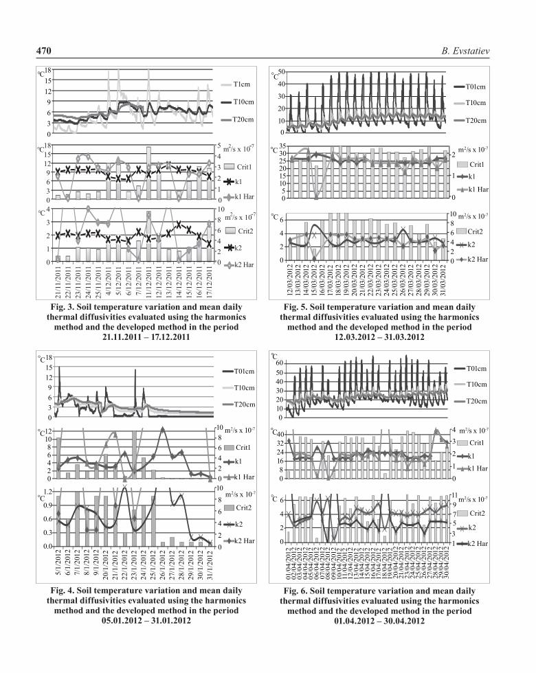
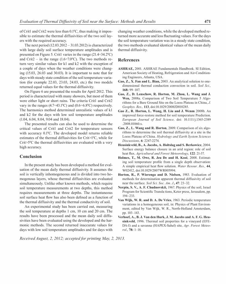
the next period (12.03.2012 – 31.03.2012) is characterized with large daily soil surface temperature amplitudes and is presented on Figure 5. Crit1 varies in the range (21.4÷34.20C) and Crit2 – in the range (1.6÷7.00C). The two methods re-turn very similar values for k1 and k2 with the exception of a couple of days when the weather conditions were chang-ing (15.03, 26.03 and 30.03). it is important to note that for days with steady state condition of the soil temperature varia-tion (for example 22.03, 23.03, 24.03, etc.) the two models returned equal values for the thermal diffusivity.

On Figure 6 are presented the results for april 2012. this period is characterized with many showers, but most of them were either light or short rains. The criteria Crit1 and Crit2 vary in the ranges (4.7÷43.10C) and (0.6÷6.80C) respectively. the harmonics method determined unrealistic values of k1 and k2 for the days with low soil temperature amplitudes (1.04, 6.04, 8.04, 9.04 and 18.04).

the presented results can also be used to determine the critical values of Crit1 and Crit2 for temperature sensors with accuracy 0.10C. the developed model returns reliable estimates of the thermal diffusivities for Crit>10C, while for Crit>50C the thermal diffusivities are evaluated with a very high accuracy.

Conclusion

in the present study has been developed a method for eval-uation of the mean daily thermal diffusivity. it assumes the soil is vertically inhomogeneous and is divided into two ho-mogenous layers, whose thermal diffusivities are evaluated simultaneously. Unlike other known methods, which require soil temperature measurements at two depths, this method requires measurements at three depths. the instantaneous soil surface heat flow has also been defined as a function of the thermal diffusivity and the thermal conductivity of soil.

an experimental study has been carried out, measuring the soil temperature at depths 1 cm, 10 cm and 20 cm. the results have been processed and the mean daily soil diffu-sivities have been evaluated using the developed and the har-monic methods. the second returned inaccurate values for days with low soil temperature amplitudes and for days with

changing weather conditions, while the developed method re-turned more accurate and less fluctuating values. For the days the soil temperature variation was in a steady state condition, the two methods evaluated identical values of the mean daily thermal diffusivity.

References

ASHRAE, 2001. asHRaE Fundamentals Handbook. si Edition, american society of Heating, Refrigeration and air-Condition-ing Engineers, atlanta, Usa.

Gao, Z., X. Fan and L. Bian, 2003. an analytical solution to one-dimensional thermal conduction convection in soil. Soil Sci., 168: 99–107.

Gao, Z., D. Lenschow, R. Horton, M. Zhou, L. Wang and J. Wen, 2008a. Comparison of Two Soil Temperature 5 Algo-rithms for a Bare Ground site on the Loess Plateau in China, J. Geophys. Res., 113, doi:10.1029/2008JD010285.

Gao Z., R. Horton, L. Wang, H. Liu and J. Wenm 2008b. an improved force-restore method for soil temperature Prediction. European Journal of Soil Science, doi: 10.1111/j.1365-2389.2008.01060.x.

Gao, Z., L. Wang and R. Horton, 2009. Comparison of six algo-rithms to determine the soil thermal diffusivity at a site in the Loess Plateau of China. Hydrology and Earth System Sciences Discussions, 6: 2247-2274.

Heusinkveld, B., A. Jacobs, A. Holtslag and S. Berkowicz, 2004. surface energy balance closure in an arid region: role of soil heat flux. Agricultural and Forest Meteorology, 122: 21-37.

Holmes, T., M. Owe, R. Jeu De and H. Kooi, 2008. Estimat-ing soil temperature profile from a single depth observation: A simple empirical heat flow solution. Water Resour. Res., 44, W02412, doi:10.1029/2007WR005994.

Horton, R., P. Wierenga and D. Nielsen, 1983. Evaluation of methods for determination apparent thermal diffusivity of soil near the surface. Soil Sci. Soc. Am. J., 47: 23–32.

Nerpin, S. V., A. F. Chudnovskii, 1967. Physics of the soil, israel Program for Scientific Transla tions, Keter press, Jerusalem, pp. 194–233.

Van Wijk, W. R. and D. A. De Vries, 1963. Periodic temperature variations in a homogeneous soil, in: Physics of Plant Environ-ment, edited by Van Wijk, W. R., North-Holland Amsterdam, pp. 103–143.

Verhoef, A., B. J. Van den Hurk, J. M. Jacobs and A. F. G. Heu-sinkveld, 1996. thermal soil properties for a vineyard (EFE-Da-i) and a savanna (HaPEX-sahel) site, Agr. Forest Meteo-rol., 78: 1–18.

Received August, 2, 2012; accepted for printing May, 2, 2013.

evaluation of thermal diffusivity of soil · pdf fileevaluation of thermal diffusivity of soil...

Documents