evaluation of hydromulches as an erosion control measure
TRANSCRIPT

Evaluation of Hydromulches as an Erosion Control
Measure Using Intermediate-Scale Experiments
by
Wesley Thurman Wilson
A thesis submitted to the Graduate Faculty of
Auburn University
in partial fulfillment of the
requirements for the Degree of
Master of Science
Auburn, Alabama
August 9, 2010
Keywords: construction, erosion, erosion-control, hydromulch, sediment, straw-mulch
Copyright 2010 by Wesley Thurman Wilson
Approved by
Wesley C. Zech, Chair, Associate Professor of Civil Engineering
Prabhakar Clement, Professor of Civil Engineering
Larry G. Crowley, Associate Professor of Civil Engineering
ii
Abstract
Discharge of sediment-laden stormwater from active construction sites, such as
highway construction projects, is a growing concern in the construction industry (Zech et
al. 2007, 2008). The United States Environmental Protection Agency (USEPA) (2009c)
has recently proposed a 280 nephelometric units (NTU) effluent limitation guideline
(ELG) pertaining to construction site runoff, and the Alabama Department of
Environmental Management (ADEM) requires construction site runoff in the state of
Alabama to retain turbidity levels within 50 NTUs above background levels. The
Alabama Department of Transportation (ALDOT) is one of many agencies in the
construction industry striving to meet the federal and state government construction site
ELGs; therefore there has been an increased interest in research efforts to test the
performance of many different erosion control practices. One such erosion control
practice, hydromulching, is the hydraulic application of mulches. Although mulching fill
slopes for erosion control is not a new practice, new technologies and innovations in the
hydromulch industry has allowed the development of superior erosion control products.
The performance of perhaps the oldest and cheapest form of erosion control,
conventional straw mulch, has been tested and reported by many researchers to be an
effective erosion control measure. However, with advancing technologies and a rise in
concern for nonpoint source (NPS) pollution flowing from construction sites into our

iii
streams, rivers, and lakes, the research of new and improved practices that reduce both
erosion and sedimentation is needed.
The purpose of this research effort was to test the intermediate-scale performance
of four hydromulches: (1) Excel® Fibermulch II, (2) GeoSkin®, (3) HydraCX2®, and
(4) HydroStraw® BFM and compare them to the performance of two conventional straw
practices, crimped or tackified, and a bare soil control. The first phase of this research
focused on researching and developing a method to accurately, uniformly, and efficiently
apply hydromulch treatments to compacted and scoured 3H:1V fill slopes that mimic
conditions similar to a highway embankment. The goal was to consistently achieve
manufacturer specified application rates through the use of scientific methods.
Ultimately, a method was developed enabling researchers to determine application rates
per spray by a hydroseeder through confirmation of collected wet and dry mulch ratios.
The second phase of this research focused on testing the performance of the four
hydromulch treatments, the two conventional straw treatments, normalized to a bare soil
condition, using 2 ft (0.6 m) wide by 4 ft (1.2 m) long test plots. Each treatment was
subject to simulated rainfall, which was divided into four 15 minute rainfall events with
15 minute breaks in between, producing a total cumulative rainfall of 4.4 inches,
representative of a 2-year, 24 hour storm event.
To determine the overall performance of each treatment, initial turbidities,
turbidity over time, and soil loss measurements were consistently collected from plot
runoff. Large amounts of collected data enabled researchers to effectively determine the
performance of each practice tested. According to experimental results from this
research effort, HydroStraw® BFM has the potential to meet ADEM ELGs of 50 NTUs,

iv
with an approximate 100% average erosion reduction and 99% average sediment
reduction when normalized to the bare soil (control) condition. Straw, tackified and
HydraCX2(R) were capable of meeting the USEPA‘s 280 NTU ELG, and on average
reduced erosion by approximately 98% and 99% respectively. Overall, the results
showed that all six practices tested were successful in controlling erosion. However, it is
recommended to use additives such as polyacrylamide (PAM) in conjunction with the six
tested practices to promote deposition and further reduce turbidity levels of construction
site discharge. The results discussed in this research are qualified by several factors such
as scale, slope, soil type, soil compaction, rainfall simulation, and rainfall intensity;
therefore the potential for biased conclusions and recommendations must be
acknowledged and may not be representative of field-scale performance.

v
Acknowledgments
The author would like to extend a special thanks to Dr. Wesley C. Zech, Dr. T
Prabhakar Clement, and Dr. Larry G. Crowley for their time and guidance throughout this
research effort. The author would also like to thank the Highway Research Center (HRC)
for funding the project, the Auburn University Civil Engineering Department for their
financial support, and everyone at the National Center for Asphalt Technology (NCAT)
Test Facility who graciously provided an innumerable amount of time and assistance
throughout the entire research project. The author would also like to thank Mr. Andrew
Rutherford, Mr. Alex Shoemaker, Mr. Wesley Donald, Mr. Jared McDonald, and Mr.
Paul Goins for the help they provided in preparing and conducting experiments. Finally,
the author would like to especially thank his parents, Kim and Betsy Wilson for
everything, because without them, none of this would have been possible.

vi
Table of Contents
Abstract ............................................................................................................................... ii
Acknowledgments............................................................................................................... v
List of Tables ..................................................................................................................... ix
List of Figures .................................................................................................................... xi
List of Abbreviations ....................................................................................................... xiv
Chapter 1 Introduction ....................................................................................................... 1
1.1 Background ................................................................................................... 1
1.2 Erosion, Sedimentation, and Turbidity ......................................................... 2
1.3 Best Management Practices (BMPs) ............................................................ 3
1.4 Research Objectives ...................................................................................... 4
1.5 Experimental Qualifications ......................................................................... 6
1.6 Organization of Thesis .................................................................................. 6
Chapter 2 Literature Review .............................................................................................. 8
2.1 Introduction ................................................................................................... 8
2.2 Environmental Regulations ......................................................................... 10
2.3 Erosion and Sediment Control (ESC) Practices.......................................... 14
2.4 Mulching ..................................................................................................... 17
2.5 Evaluation of straw Mulch Practices .......................................................... 29
2.6 Literature Review Summary ....................................................................... 39

vii
Chapter 3 Intermediate-Scale Test Methods and Procedures .......................................... 42
3.1 Introduction ................................................................................................. 42
3.2 Intermediate-Scale Testing ......................................................................... 42
3.3 Experimental Design ................................................................................... 46
3.4 Experimental Procedures Pre-Condition Application ................................. 52
3.5 Condition Application Experimental Procedures ....................................... 63
3.6 Data Collection ........................................................................................... 82
3.7 Statistical Analyses ..................................................................................... 85
3.8 Summary ..................................................................................................... 86
Chapter 4 Intermediate-Scale Experiments Results and Discussion ............................... 88
4.1 Introduction ................................................................................................. 88
4.2 Experimental Results .................................................................................. 88
4.3 Summary ................................................................................................... 112
Chapter 5 Conclusions and Recommendations .............................................................. 116
5.1 Introduction ............................................................................................... 116
5.2 Intermediate-Scale Test Methods and Procedures .................................... 117
5.3 Performance of Conventional Straw and Hydromulch ............................. 118
5.4 Recommended Future Research ............................................................... 121
References ....................................................................................................................... 123
Appendix 1 Manufacturer‘s Specifications for Rainfall Simulator Components .......... 129
Appendix 2 Rainfall Intensity-Duration-Frequency Curves for Alabama. .................... 135
Appendix 3 Manufacturer‘s Specs for Equipment Used During Experimentation ....... 138
Appendix 4 Hydromulch Manufacturer Specifications ................................................. 142
viii
Appendix 5 Hydromulch Experimentation .................................................................... 148
Appendix 6 Experimental Results ................................................................................. 157
Appendix 7 Statistical Analysis ..................................................................................... 172

ix
List of Tables
Table 1.1 Summary of Different BMPs for Protecting Against Erosion, Sedimentation,
and Stormwater Discharge ................................................................................. 3
Table 2.1 USEPA Menu of BMPs and Reported Cost and Effectiveness ....................... 16
Table 2.2 Mulching Materials and Application Rates ..................................................... 18
Table 2.3 Types of Hydraulically Applied Erosion Control Products (HECPs) ............. 24
Table 2.4 Product Specifications used in this Research .................................................. 27
Table 2.5 Summary of Reviewed Straw Mulch Practices ............................................... 33
Table 2.6 Summary of Reviewed Hydromulch Practices ................................................ 38
Table 3.1 Percent Composition and Classification of Experimental Soil ........................ 52
Table 3.2 Calculated Dry Unit Weight (pcf) and Required Number of Drops ................ 56
Table 3.3 Assigned Hydromulch and Classification........................................................ 57
Table 3.4 Determination of Number of Sprays for Required Application Rate .............. 76
Table 3.5 Determined Number of Sprays For Hydromulch Products Tested .................. 78
Table 3.6 Breakdown of Collected Data Totals ............................................................... 84
Table 4.1 Average Initial Turbidity Results for Surface Runoff ..................................... 92
Table 4.2 Tukey-Kramer Comparison on Average Initial Turbidity ............................... 94
Table 4.3 Summary of Average Turbidity vs. Time Measurements................................ 99
Table 4.4 Average Soil Loss due to Surface Runoff [Straw, Crimped or Tackified;
Excel®Fibermulch II] .................................................................................... 105

x
Table 4.5 Average Soil Loss due to Surface Runoff [GeoSkin®, HydraCX2®,
HydroStraw®] ................................................................................................ 105
Table 4.6 Tukey-Kramer Comparison on Average Soil Loss........................................ 107
Table 4.7 Cumulative Soil Loss (A) to Calculate Cover Factors (C) per Treatment..... 112

xi
List of Figures
Figure 2.1 Commercial Straw-Blower. ............................................................................ 19
Figure 2.2 Straw-Crimper. ............................................................................................... 21
Figure 2.3 Proposed ALDOT (2009) Minimum Requirements and Classifications ....... 26
Figure 3.1 Test Facility Exterior. ..................................................................................... 44
Figure 3.2 Test Facility Interior. ...................................................................................... 44
Figure 3.3 Illustrations of TurfMaker® 380 and Various Features. ................................ 45
Figure 3.4 Comparison of Collection Devices. ................................................................ 46
Figure 3.5 Sideboards Installed on Test Plots. ................................................................. 48
Figure 3.6 3H:1V Slope using Cinderblocks and Saw Horses. ....................................... 48
Figure 3.7 Illustration of Rainfall Simulator.................................................................... 50
Figure 3.8 Illustration of Simulator Relative to Plots. ..................................................... 50
Figure 3.9 Proctor Curve for Experimental Soil. ............................................................. 53
Figure 3.10 Mold used to Determine Required Compaction Rate with Hand-Tamp. ..... 54
Figure 3.11 Compaction of Soil Using Hand................................................................... 55
Figure 3.12 Flowchart of Experimental Organization. .................................................... 59
Figure 3.13 5 and 3 Gallon Bucket Used to Load Test Plots. .......................................... 61
Figure 3.14 8 Sections to Compact Approximately 80 Times. ........................................ 62
Figure 3.15 Uniform Tilling of Surface Approximately ¼ inch in Depth. ...................... 62
Figure 3.16 Mechanically Blown Straw. ......................................................................... 64

xii
Figure 3.17 Mulch Crimper. ............................................................................................ 65
Figure 3.18 Weighing and Applying Conventional Straw................................................ 66
Figure 3.19 Intermediate-Scale Mulch Crimper Design and Construction Process. ....... 67
Figure 3.20 Crimping Straw. ........................................................................................... 68
Figure 3.21 Hytac II—Tackifier for Convetional Straw. ................................................. 69
Figure 3.22 Mixing and Application of Hytac II Tackifier to Conventional Straw. ....... 70
Figure 3.23 Conventional Straw with Tackifier for 48 hr Drying Period. ....................... 71
Figure 3.24 3H:1V Test Boards Pre-Application of Hydromulch. .................................. 72
Figure 3.25 After One Spray to Each Test Board. ........................................................... 73
Figure 3.26 Applying Second Spray to Boards 2 through 8. ........................................... 73
Figure 3.27 Post Application of 1-8 Sprays on Test Boards 1-8. .................................... 74
Figure 3.28 Post Application—Scraping Boards into Bucket for Weighing. .................. 74
Figure 3.29 Hydromulch Scraped off of Test Boards into Corresponding Buckets. ....... 74
Figure 3.30 Scatter Plots of Wet Unit Weight vs. Number of Sprays ............................. 77
Figure 3.31 Scraping First Two Test Boards. .................................................................. 79
Figure 3.32 First Two Plots Scraped For Weighing. ....................................................... 79
Figure 3.33 Wooden Structure to Suspend Heat Lamps. ................................................. 81
Figure 3.34 Heat Lamps Measured for Accurate Spacing. .............................................. 81
Figure 3.35 Collection of Runoff. .................................................................................... 83
Figure 3.36 Turbidity Over Time..................................................................................... 83
Figure 3.37 Filtering Process. .......................................................................................... 84
Figure 4.1 Average Initial Turbidity of Surface Runoff vs. Time. .................................. 89
Figure 4.2 Average Initial Turbidity of Surface Runoff vs. Time w/o Control. .............. 90

xiii
Figure 4.3 Average Recorded Turbidity for all Samples vs. Time. ................................. 95
Figure 4.4 Straw Treatments‘ Average Recorded Turbidity from 5 to 10 Minute
Samples. .......................................................................................................... 97
Figure 4.5 Hydromulch Treatments‘ Average Recorded Turbidity from 5 to 10 Minute
Samples ........................................................................................................... 98
Figure 4.6 Average Soil Loss vs. Time.......................................................................... 101
Figure 4.7 Average Cumulative Soil Loss vs. Time. ..................................................... 103
Figure 4.8 Average Initial Turbidity vs. Average Eroded Soil. ..................................... 108
Figure 4.9 Average Initial Turbidity vs. Average Eroded Soil [Excludes Control]. ..... 110
Figure 4.10 Average Percent Reduction of Treatments Compared to Control. ............. 114

xiv
List of Abbreviations
ADEM Alabama Department of Environmental Management
ALDOT Alabama Department of Transportation
ANOVA Analysis of Variance
ASTM American Society for Testing and Materials
ASWCC Alabama Soil and Water Conservation Committee
BFM Bonded Fiber Matrix
BMP Best Management Practices
CWA Clean Water Act
ECP Erosion Control Product
ECTC Erosion Control Technology Council
ELG Effluent Limitation Guideline
ESC Erosion and Sediment Control
FRM Fiber Reinforced Matrix
HECP Hydraulically Applied Erosion Control Product
HM Hydraulic Mulch
IDF Intensity Duration Frequency
MBFM Mechanically Bonded Fiber Matrix
MC Moisture Content
NCAT National Center for Asphalt Technology

xv
NPDES National Pollution Discharge Elimination System
NPS Non-point Source
NTU Nephelometric Units
OMC Optimum Moisture Content
PAM Polyacrylamide
SHA State Highway Agency
SLR Soil Loss Ratio
SMM Stabilized Mulch Matrix
USEPA United States Environmental Protection Agency

1
Chapter 1 Introduction
1.
1.1 Background
Discharge of sediment-laden stormwater from active construction sites, such as highway
construction projects, is a growing concern in the construction industry (Zech et al. 2007,
2008). The United States Environmental Protection Agency (USEPA) labels such
discharge as nonpoint source (NPS) pollution and is defined as land runoff, precipitation,
atmospheric deposition, seepage or hydrologic modification that does not meet the legal
definition of ‗point source‘ in section 502(14) of the Clean Water Act. NPS pollution can
include bacteria, oil, grease and toxic chemicals, excess fertilizers from agricultural
runoff, salt from irrigation practices, and sediment from improperly managed
construction sites (USEPA, 2008). According to the USEPA‘s Storm Water Phase II
Final Rule Fact Sheet Series (2008), sedimentation from construction site runoff is one of
the most widespread pollutants affecting rivers and streams, second only to pathogens
(i.e., bacteria). In an effort to reduce erosion and sedimentation, the USEPA has
implemented a numeric limitation of 280 nephelometric units (NTUs) to be phased in
over the next four years, beginning in August of 2011, for construction sites that disturb
10 or more acres at a time (USEPA, 2009c). In addition to federal guidelines, the
Alabama Department of Environmental Management (ADEM), with authority given by
the federal government, has implemented effluent limitation guidelines (ELGs)

2
forbidding construction sites in the State of Alabama not to exceed runoff turbidities of
50 NTUs above background levels. These federal and state guidelines have encouraged
the construction industry to establish a scientific approach to evaluate the performance of
erosion and sediment control (ESC) practices in reducing erosion rates and turbidity
levels.
1.2 Erosion, Sedimentation, and Turbidity
Erosion and sedimentation produced by construction site runoff is a main contributor of
NPS pollution in the construction industry. ―The erosion process is influenced primarily
by climate, topography, soils, and vegetative cover‖ (ASWCC, 2009). Erosion,
sedimentation, and turbidity can be described as a chain reaction; erosion of land leads to
sediment transport in stormwater runoff, which in turn causes water to become turbid,
eventually resulting in sedimentation as water velocities decrease. Erosion is defined by
the Alabama Soil and Water Conservation Committee (ASWCC) as the ―process by
which the land surface is worn away by the action of water, wind, ice or gravity‖
(ASWCC, 2009). Sedimentation can be defined as ―the process that describes soil
particles settling out of suspension as the velocity of water decreases‖ (ASWCC, 2009).
Turbidity occurs as sediment particles are being transported in stormwater runoff, causing
water to become turbid, cloudy, or muddy prior to deposition. High levels of turbidity in
rivers, streams, and lakes can have severe negative impacts (e.g., killing fish from gill
abrasion, decreasing light penetration, smothering food sources, etc.) on the environment
and wild life (ASWCC, 2009).

3
Although the ASWCC (2009) states that it is difficult, perhaps impossible, to totally
eliminate the transport of clay and silt particles even with the most effective ESC
practices, research and evaluation of ESC products is required to minimize NPS pollution
discharges from construction sites to acceptable levels.
1.3 Best Management Practices (BMPs)
Federal and state ELGs have encouraged the construction industry to develop best
management practices (BMPs) in an effort to effectively control erosion and
sedimentation caused by construction site runoff. BMPs are methods that have been
determined to be the most effective, practical means of preventing or reducing pollution
from NPS pollution. A list of BMPs has been developed by ASWCC (2009) to guide
contractors in properly selecting the BMP or combination of BMPs for specific
construction site circumstances. The list is summarized below in Table 1.1.
Table 1.1 Summary of Different BMPs for Protecting Against Erosion,
Sedimentation, and Stormwater Discharge
BMP
Categories Types Best Management Practices
Surface
Stabilization
Chemical Stabilization; Erosion Control Blankets; Mulching;
Permanent Seeding; Retaining Walls; Sodding;
Runoff
Conveyance
Check Dams; Diversions; Drop Structures; Outlet Protection;
Subsurface Trains; Swales
Sediment
Control
Brush/Fabric Barriers; Drop Inlet Protection; Filter Strips; Floating
Turbidity Barriers; Inlet Protection; Sediment Barriers; Sediment
Basins; Sediment Traps
Stormwater
Management Bioretention Area; Porous Pavement; Stormwater Detention Basins
Stream
Protection
Buffer Zones; Channel Stabilization; Stream Diversion Channel;
Streambank Protection; Temporary Stream Crossings

4
The BMPs listed in Table 1.1 are a sample of specific BMPs that can be implemented to
prevent pollution from construction generated NPS. This study will focus on
hydraulically applied mulch, referred herein as hydromulch, which inherently falls under
the ‗Surface Stabilization‘ BMP category. The Alabama Department of Transportation
(ALDOT) specifications for Mulching and Vegetation Establishment state that a
hydromulch ―shall be manufactured in such a manner that after addition and agitation in
slurry tanks with soil amendments, the fibers in the material will become uniformly
suspended to form a homogenous slurry; and that when hydraulically sprayed on the
ground, the material will form a ground cover; and which after application will allow the
absorption of moisture and allow rainfall or mechanical watering to percolate to the
underlying soil‖ (ALDOT, 2008). Technological advancements in methods of
application and mixing hydromulches has provided the construction industry with tools to
manufacture new hydromulches that claim to be superior to traditional erosion control
practices such as conventional straw mulch. However, since available scientific
knowledge is limited, it is desirable to conduct performance-based intermediate-scale
tests to quantify hydromulch erosion control efficiencies.
1.4 Research Objectives
This research effort is an extension of the erosion and sediment control study conducted
by the Highway Research Center at Auburn University in conjunction with ALDOT to
further the collective knowledge of BMPs on highway construction sites. This study
incorporated test methods and protocols used by Shoemaker et al. (2009). Tests were

5
conducted at an ESC facility located on the premises of the National Center for Asphalt
Technology (NCAT) near Opelika, AL.
The overall objective of this research effort was to test the erosion control performance of
the following four hydromulch practices: (1) Excel® Fibermulch II, (2) GeoSkin®, (3)
HydraCX2®, and (4) HydroStraw® BFM. A comparative analysis will be conducted to
quantify performance by comparing the hydromulch practices to bare soil and two
conventional straw treatments: (1) conventional straw, crimped and (2) conventional
straw, tackified. To accurately test these six erosion control practices, this study was
divided into two phases: (1) experimental preparations and (2) experimentation and
evaluation.
PHASE 1: EXPERIMENTAL PREPARATIONS
1. Design and construct a flume that modifies Shoemaker‘s (2008) runoff collection
device.
2. Research and develop a uniform and consistent method of applying conventional
straw that is crimped or tackified.
3. Research and develop uniform and consistent methods of applying each
hydromulch tested to ensure manufacturer specified application rates are
achieved.
PHASE 2: EXPERIMENTATION & EVALUATION
1. Examine the effectiveness of and the four selected hydromulches for use as an
erosion control measure on a compacted, 3:1 slope.

6
2. Analyze the results to provide scientific-data-based recommendations for
hydromulching on highway construction sites.
1.5 Experimental Qualifications
There are five qualifying experimental factors that may have an impact on conclusions
that are drawn from the results reported from this research, which include: (1) soil type,
(2) slope, (3) soil compaction, (4) rainfall simulator, and (5) rainfall intensity. These
qualifying factors were designed into the experimental procedures and have the potential
to create a biased outcome on some conclusions and recommendations that can be made
for erosion control practices tested. It should also be noted the intermediate-scale results
reported herein may not be scale-able to field-scale or practical-scale performance on
active construction sites.
1.6 Organization of Thesis
This thesis is divided into five descriptive chapters to present and explain the steps taken
to complete the objectives of this research. Following this chapter, Chapter 2: Literature
Review will explain conventional straw mulching practices, introduce and define different
types of hydromulch as well as the hydromulches tested in this research effort, and
review previous studies conducted on conventional straw and hydromulch practices.
Chapter 3: Intermediate-Scale Methods and Procedures, will present the design and
development of the intermediate-scale testing procedures and protocols. Chapter 4:
Experimental Results will compare and analyze the data collected from the experiments,
including an ANOVA statistical analysis performed for determination of significance
between bare soil, conventional straw, and hydromulch treatments. Chapter 5:

7
Conclusions and Recommendations combines the data, results, and analyses conducted
throughout this research effort to develop scientifically-based recommendations for the
performance and use of each hydromulch. These recommendations will aid ALDOT in
selecting proper types and applications of hydromulch products on highway construction
sites with the goal of complying with federal and state effluent limitations.
.
8
Chapter 2 Literature Review
2.
2.1 Introduction
The process of urbanization (e.g. construction of highways, buildings, farms, parking
lots, residential developments, etc.) modifies the natural orientation of the land and
environment. Therefore when a rainfall event occurs, the path by which water flows to
rivers, lakes and streams is ultimately altered. These unnatural, impervious altercations
to the earth‘s surface cause an increase in total runoff volumes. When large, concentrated
volumes of water traverse over areas disturbed by construction, there is an increased risk
for erosion.
―Both falling rain and flowing water, typically referred to as stormwater, perform work in
detaching and moving soil particles‖ (ASWCC, 2009), herein referred to as soil erosion.
Soil erosion is considered the largest contributor to non-point source pollution in the U.S.
(USEPA, 1997). An estimated $27 billion annually is spent in the U.S. in an effort to
control soil erosion (Brady and Weil, 1996). It is also reported that soil loss rates are 20
times greater from construction sites than agricultural lands, and 1,000 to 2,000 times
greater than forest lands (USEPA, 2005b). When soil is eroded from construction sites,
other harmful particulates such as fertilizers, pesticides and fuels attach to the soil and are
transported into municipal storm sewer systems (MS4s) (Risse and Faucette 2001;

9
USEPA, 2005a). Polluted stormwater systems transport construction site runoff directly
to surface waters, ultimately causing sedimentation. ―Sedimentation impairs 84,503 river
and stream miles (12% of the assessed river and stream miles and 31% of the impaired
river and stream miles)‖ (USEPA, 2000). Sedimentation of surface water can lead to
deterioration of aquatic habitats, rapid loss of storage capacity of reservoirs, eroded
streambanks, and increased turbidities of the waters, reducing photosynthesis and
clogging fish gills (Novotny, 2003). An annual estimate of $17 billion is spent in the
U.S. alone in an effort to control sedimentation, bringing the national total to over $44
billion in erosion and sediment control (Brady and Weil, 1996). Thus, the combination
of environmental and economic downfalls related to erosion and sedimentation in the
construction industry has developed a need for scientific research to be performed to
understand the overall performance of ESC practices used at the federal, state, and local
levels.
The primary goal of this research was to develop intermediate-scale experimental
procedures to test the performance of hydromulches as an erosion control practice on a
typical 3H:1V highway construction slope. This research effort and its stated objectives
discussed in Section 1.4 were established in an effort to gain scientific knowledge on the
performance of several hydromulch products relative to bare soil and conventional straw
practices. Typical highway construction sites rely heavily upon the success of ESC
practices to control erosion and sedimentation while complying with USEPA regulations.
Thus the research conducted herein will provide ALDOT with scientific findings

10
regarding performance characteristics of erosion control products for use on future
construction projects.
Before these research objectives can be satisfied, it is pertinent to conduct a thorough
literature review. The literature review herein will focus on identifying: (1) federal,
state, and local environmental regulations specific to construction site ESC, (2) a review
of erosion control practices, specifically conventional straw and hydromulches, and (3)
previous literature related to conventional straw and hydromulch tests.
2.2 Environmental Regulations
The USEPA has developed ELGs to establish national standards for the regulation of
construction stormwater runoff, which are the minimum standards state highway agencies
(SHAs) are required to comply with. However, if a state chooses to impose stricter
regulations than the required federal regulations and attain permission by the federal
government to do so, then they have mandate to enforce higher effluent standards. This
section will discuss a brief history of regulating our nation‘s waters, present USEPA
environmental guidelines, and the ELGs required by the state of Alabama, upheld by
ADEM.
2.2.1 USEPA Regulations
In 1899, the United States made its first federal action towards protecting our nation‘s
waters with the Refuse Act. This act outlawed the ―dumping of refuse that would
obstruct navigation of navigable waters, except under a federal permit,‖ which would in

11
the 1960‘s be redefined to cover industrial waste (USEPA, 2010a). It wasn‘t until 1972
that the National Pollution Discharge Elimination System (NPDES) was created in
section 402 of the Clean Water Act (CWA), prohibiting the discharge ―of pollutants from
any point source into the nation‘s waters except as allowed under an NPDES permit‖
(USEPA, 2010a). Five years later, Congress amended the CWA to focus on controlling
toxic discharge, and in 1987 Congress passed an act calling for the increased monitoring
of water bodies to ensure water quality standards were upheld by on-site construction
contractors (USEPA, 2010a).
In 1990, Phase I of the USEPA stormwater program was promulgated under the CWA,
relying on the NPDES ―permit coverage to address stormwater runoff from: (1) ‗medium‘
and ‗large‘ municipal separate storm sewer systems (MS4s) generally serving populations
of 100,000 or greater, (2) construction activity disturbing 5 acres of land or greater, and
(3) ten categories of industrial activity‖ (USEPA, 2005a). In 1999, the Stormwater Phase
II final rule expanded Phase I by implementing six measures, which in summary required
―additional operators of MS4s in urbanized areas and operators of small construction
sites, through the use of NPDES permits, to implement programs and practices to control
polluted stormwater runoff‖ (USEPA, 2005a). Despite Phase I and Phase II‘s ESC
efforts, the 2000 National Water Quality Inventory (USEPA, 2000) reported that in the
U.S., approximately 40% of surveyed water bodies are still impaired, and 13% of
impaired rivers, 18% of impaired lake acres and 32% of impaired estuaries were still
affected by urban/suburban stormwater runoff.

12
In 2009, the USEPA released a full national economic and environmental analysis of
ELGs for the construction industry in the Economic Analysis of Final Effluent Limitation
Guidelines and Standards for the Construction and Development (USEPA, 2009a) and
the Environmental Impact and Benefits Assessment for Final Effluent Guidelines and
Standards for the Construction and Development Category (USEPA, 2009b). These two
documents were the basis of support for the Final Rule: Effluent Guidelines for
Discharge from the Construction and Development Industry, which promulgated ELGs
and new source performance standards (NSPS) to control the discharge of pollutants from
construction sites (USEPA, 2009c). In summary, this final rule contains stringent
requirements for soil stabilization, acquiring NPEDS permits, and implementation of
ESC practices. Also, the USEPA is implementing a numeric limitation of 280 NTUs to
be phased-in over the next four years, beginning in August of 2011 to ―allow permitting
authorities adequate time to develop monitoring requirements and to allow the regulated
community time to prepare for compliance with the numeric limitation.‖ (USEPA,
2009c). This rule states ―construction sites that disturb 20 or more acres at one time will
be required to conduct monitoring of discharges and comply with the numeric limitation
beginning 18 months after the effective date of the final rule‖ (USEPA, 2009c). Also, it
states that after the four years, the 280 NTU limitation will apply to construction sites
disturbing 10 or more acres at one time. In the USEPA‘s costs and benefits analysis
(2009c), it was estimated that approximately 4 billion pounds of sediment discharged
from construction sites will be reduced, saving about $953 million annually, once this
final rule reaches final implementation.

13
2.2.2 The State of Alabama Regulations
Alabama is an authorized state, meaning the USEPA has given the State of Alabama
permission to administer state environmental regulations in lieu of most federal
environmental regulations (ADEM, 2010a). One such federal environmental regulation
Alabama has permission to administer is the standards regarding water quality of water
bodies within the State. ADEM is responsible for ensuring federal regulations are
followed. Therefore, in Division 6, Volume 1 of their rules and regulations, ADEM
―prescribes regulations for development and implementation of water quality standards
and water body use classifications for all waters of the State; prescribes conditions
relevant to the issuance of permits to include effluent limitations for each discharge for
which a permit is issued; and such other rules as necessary to enforce water quality
standards. Within ADEM‘s water quality program, Chapter 335-6-10 Water Quality
Criteria (2010b), they require ―no turbidity other than natural origin that will cause
substantial visible contrast with the natural appearance of waters or interfere with any
beneficial uses which they serve. Furthermore, in no case shall turbidity exceed 50 NTU
above background levels. Background levels will be interpreted as the natural condition
of receiving waters without the influence of man-made or man-induced causes. Turbidity
caused by natural runoff will be included in establishing background levels.‖
Although the USEPA is phasing in a 280 NTU effluent guideline, the 50 NTU regulation
from ADEM overrules in the State of Alabama. Therefore, for ALDOT and the research
herein, 50 NTU above background levels is the numerical guideline followed.

14
2.3 Erosion and Sediment Control (ESC) Practices
The USEPA defines BMPs as ―a technique, process, activity, or structure used to reduce
the pollutant content of a storm water discharge.‖
It is important to identify the length of time a BMP is expected to perform. Erosion
control products (ECPs) can be divided into two categories: short term and permanent
ECPs. The Erosion Control Technology Council (ECTC) defines short term ECPs as
products ―designed to provide erosion protection for longer than three months and up to
12 months,‖ which is basically one growing season for the establishment of vegetation
(ECTC, 2008). Permanent ECPs can be defined as a product designed to provide
permanent, long term protection from erosion. Typical short term ECPs are erosion
control blankets, spray-emulsion products (i.e., hydromulches), and straw mulches, where
the best long term control is well established vegetation (Benik et al., 2003). The focus
of this research is on short term, temporary performance of ECPs.
The USEPA (2006) has developed a menu of BMPs for erosion and sediment control on
construction sites along with their reported cost and effectiveness from previous
researchers, shown in Table 2.1. According to Table 2.1, the most common BMPs in the
erosion control industry today are chemical stabilizers with a 70% to 90% efficiency rate,
compost blankets with a 70% to 100% efficiency rate, geotextiles, gradient terraces,
mulching with a 53% to 99.8% efficiency rate, seeding with an average efficiency rate of
90%, and sodding with an average efficiency rate of 99%. As reported by the USEPA

15
(2006), these are all efficient forms of ESC; however the focus in this research effort is
on mulching practices such as conventional straw and hydraulically applied mulches.

16
Table 2.1 USEPA Menu of BMPs and Reported Cost and Effectiveness
BMPs* Description Cost1, 2
Effectiveness
Chemical Stabilizers Soil binders or soil palliatives, provide temporary soil stabilization. $4-$35/lb 70-90%
(Aicardo, 1996)
Compost Blankets A layer of loosely applied compost or composted material that is placed on the
soil in disturbed areas to control erosion and retain sediment resulting from sheet-
flow runoff.
$0.83-$4.32/yd3
(Faucette, 2004)
70-100%
(Faucette and Risse, 2002)
Geotextiles
(RECPs)
Manufactured by weaving or bonding fibers that are often made of synthetic
materials such as polypropylene, polyester, polyethylene, nylon, polyvinyl
chloride, glass, and various mixtures of these materials. As a synthetic
construction material, geotextiles are used for a variety of purposes such as
separators, reinforcement, filtration and drainage, and erosion control (USEPA,
1992).
$0.50-$10/yd2
(SWRCP, 1991)
n/a
Gradient Terraces Earthen embankments or ridge and channel systems that reduce erosion by
slowing, collecting and redistributing surface runoff to stable outlets that increase
the distance of overland runoff flow.
n/a n/a
Mulching An erosion control practice that uses materials such as grass, hay, wood
chips, wood fibers, straw, or gravel to stabilize exposed or recently planted
soil surfaces.
$800-$3500/acre
(USEPA, 1993)
53-99.8%
(Harding, 1990)
Riprap A layer of large stones used to protect soil from erosion in areas of concentrated
runoff.
$35-$60/yd2
(Mayo et al., 1993)
n/a
Seeding Used to control runoff and erosion on disturbed areas by establishing perennial
vegetative cover from seed.
$200-$1000/acre
(USEPA, 1993)
50-100% (90% avg.)
(USEPA, 1993)
Sodding A permanent erosion control practice and involves laying a continuous cover of
grass sod on exposed soils.
$0.10-$1.10/ft2
(USEPA, 1993)
99%
Note: ‗*‘ Source: USEPA, 2010b
‗1‘ 1 lb = 0.45 kg
‗2‘ 1 ft = 0.31 m

17
2.4 Mulching
According to the USEPA (2006), ―mulching is an erosion control practice that uses
materials such as grass, hay, wood chips, wood fibers, straw or gravel to stabilize
exposed to or recently planted soil surfaces.‖ The Alabama Handbook for Erosion
Control, Sediment Control and Stormwater Management on Construction Sites and
Urban Areas (2009) states that ―surface mulch is the most effective, practical means of
controlling runoff and erosion on disturbed land prior to vegetation establishment;‖
however is most effective when used in conjunction with vegetation (USEPA, 2006). As
shown in Table 2.1, one of the most expensive types of erosion control is mulching;
nonetheless, mulches report a maximum potential of 99.8% efficiency. Lancaster and
Theisen (2004) recall that although methods of ESC practices such as mulching are
expensive, ―expense and performance increase with the level of engineering.‖
Researchers (Box and Bruce, 1996; Bruce et al., 1995; Sutherland, 2006, 1998) have
reported that mulches used to control erosion have a two-fold advantage, having the
capability to reduce soil loss while protecting grass seeds and soil amendments from
being washed away. Additionally, mulches are also capable of reducing solar radiation,
suppress fluctuations of soil temperature, reduce water loss through evaporation, dissipate
rainfall impact, and help prevent soil crust formation (Sutherland, 1998; 1986; Rickson,
1995; Turgeon, 2002; Singer et. al 1981; Bruce et. al. 1995).
Table 2.2 shows typical mulching materials and application rates used in Alabama
(ASWCC, 2009; USEPA, 2006). In summary, the table represents application rates and

18
guidelines for conventional straw with and without seed, wood chips, bark, pine straw,
and peanut hulls.
Table 2.2 Mulching Materials and Application Rates
(Source: ASWCC, 2009)
Mulch Rate Per Acre and (Per 100 ft2)
1 Guidelines
Conventional
Straw with Seed 1.5-2 tons (70 lbs-90 lbs)
Spread by hand or machine to attain 75%
groundcover; anchor when subject to blowing.
Conventional
Straw (no seed) 2.5-3 tons (115 lbs-160 lbs)
Spread by hand or machine; anchor when
subject to blowing.
Wood Chips 5-6 tons (225 lbs-270 lbs) Treat with 12 lbs. nitrogen/ton.
Bark 35 cubic yards Can apply with mulch blower.
Pine Straw 1-2 tons (45 lbs-90 lbs) Spread by hand or machine; will not blow like
straw.
Peanut Hulls 10-20 tons (450 lbs-900 lbs) Will wash off slopes. Treat with 12 lbs.
nitrogen/ton.
Notes: ‗1‘ 1 lb = 0.45 kg; 1 ton = 0.89 metric tons
When selecting the proper mulch to apply to a slope for erosion control, the mulch should
be based on soil conditions, slope steepness and length, season, type of vegetation
established, and size of the area (ASWCC, 2009; USEPA, 2006). Mulches such as wood
chips are often highly considered as an erosion control measure when germination is not
an option. Wood chips do not require tacking, but they decompose slowly, requiring a
treatment of 12 pounds (5.44 kg) of nitrogen per ton to prevent nutrient deficiency in
plants.
Although there are several adequate mulches for erosion control on highway construction
slopes, illustrated in Table 2.2, the focus in this research effort is on conventional straw
practices and hydraulically applied mulches. The following sections of the literature

19
review will report on: (1) conventional straw erosion control practices and (2) typical
hydraulically applied mulches.
2.4.1 Conventional Straw Erosion Control Practices
The purpose of testing conventional straw herein was to have a traditional, low-cost,
widely used ESC practice to compare to the performance of hydromulch products. Straw
is considered one of the most common ground covers used to reduce erosion on
construction sites (ASWCC, 2009), and as shown in Table 2.1, has been reported to
reduce erosion rates by more than 90 percent if applied at sufficient rates (Mannering and
Meyer, 1963; McLaughlin and Brown, 2006; Meyer et al., 1970; Singer et al.,1981).
Turgeon (2002) states that straw is also capable of encouraging grass establishment by
reducing runoff, increasing infiltration, and improving soil conditions. Advancements in
technology have made the application of conventional straw a simple and unproblematic
procedure. The application of conventional straw on large construction sites can be
achieved with commercial blowers that break up straw bales and blow the straw onto the
soil, illustrated in Figure 2.1.
Figure 2.1 Commercial Straw-Blower. (Source: http://www.revolutionequipment.com.au/strawblower-gallery.html)

20
The Alabama Handbook for Erosion Control, Sediment Control and Stormwater
Management on Construction Sites and Urban Areas (2009) requires approximately 75%
ground cover when applying conventional straw. Straw‘s performance depends heavily
upon the contractor for achieving consistent, uniform application and coverage of straw
on the soil surface. If application of the straw is inconsistent, the performance of the
installation will be compromised (Babcock et al., 2008; Lancaster et al., 2006).
Conventional straw is also effectively applied by hand, which was the application method
used for the research herein; however, this method can become very costly when applied
at a large scale due to labor costs (Babcock et al., 2008). When applying straw by hand,
it is encouraged to ―divide the area into sections of approximately 1,000 ft2 (92.9 m
2) and
place 70 to 90 pounds (31.8 to 40.8 kg) of straw (1½ to 2 bales) in each section to
facilitate uniform distribution‖ (ASWCC, 2009). Conventional straw is very lightweight,
therefore it is susceptible to wind erosion, and needs to be immediately anchored with a
mulch anchoring tool such as a mulch crimping machine, shown in Figure 2.2, or
tackifiers (ALDOT, 2008; ASWCC, 2009; Babcock et al., 2008; USEPA, 2006).

21
Figure 2.2 Straw-Crimper. (Source: http://www.mulchers.com/images/straw-crimper.jpg)
Straw crimpers are typically used to crimp or punch straw into the soil when the soil is
not too sandy (Babcock et al., 2008). ALDOT (2008) classifies straw mulch placed on
3H:1V or flatter slopes using a crimper as a ―Class A, Type 1‖ mulch. If crimpers are not
available or necessary, liquid mulch binders are used to ‗tack‘ mulch by spraying them
over the straw, but applying straw and binder together is the most effective method
(ASWCC, 2009). ALDOT (2008) specifies straw mulch that requires an adhesive and
shall be used on slopes steeper than 3H:1V are classified as ―Class A, Type 2‖ mulches.
―Emulsified asphalt is the most commonly used mulch binder‖ (ASWCC, 2009);
however wood and paper fiber hydromulches, guar, and starch-based tackifiers are also
commonly used to bind straw (Babcock et al., 2008).
22
There are advantages and disadvantages to using straw mulch for erosion control. The
advantages are that it is inexpensive, quick and easy to apply using a straw-blower,
capable of achieving efficient grass growth, and no water is needed for application.
Conversely, disadvantages of conventional straw include that it does not effectively
prevent soil loss as well as more expensive erosion products, is susceptible to wind
erosion if not properly anchored, may introduce weed seeds, and fines from straw-
blowers can drift long distances (Babcock et al., 2008).
2.4.2 Hydraulically Applied Mulch (a.k.a. Hydromulch)
It has been reported that field practices, such as blown straw, slope interruptions, or
gradient terraces, represent the least expensive and least reliable form of erosion control,
whereas ―an application of a loose or hydraulically applied mulch cover represents an
upgraded level of performance,‖ and provide the highest level of erosion control and
confidence (Lancaster et al., 2006). Hydraulically applied mulches, referred to herein as
‗hydromulches‘, have shown continuous evolution and improvement over the past 50
years. Advancements in technology have resulted in the production of equipment and
materials that offer enhanced performance and greater productivity over many traditional
methods of erosion control. There is a knowledge gap between the cost-effectiveness and
performance benefits of new products (Morgan and Rickson, 1988; NCHRP, 1980;
Sutherland, 1998; Weggel and Ruston, 1992) such as hydromulches, largely due to newly
evolving technologies as well as a lack of research involving hydromulch products.

23
The introduction of water, refined fiber matrices, tackifiers, super-absorbents,
flocculating agents, man-made fibers, plant biostimulants and other performance
enhancing additives as a hydromulch practices on slopes has forced federal, state, and
local governments to begin developing hydromulch guidelines. The American Society
for Testing and Materials (ASTM) has proposed new standards for testing hydraulically
applied erosion control products (HECPs). Also, ECTC has divided HECPs into four
distinct categories, relevant to their corresponding functional longevity, erosion control
effectiveness, and vegetative establishment, illustrated in Table 2.3 (ECTC, 2008;
Babcock et al., 2008).

24
Table 2.3 Types of Hydraulically Applied Erosion Control Products (HECPs)
Slope Ratio Material Rate
1
(lbs/acre) Description
≤2H:1V Stabilized Mulch Matrix (SMM) 1,500-2,500 Organic fibers with soil flocculants or cross-linked hydro-
colloidal polymers or tackifiers. Used to provide erosion control
and facilitate vegetative establishment on moderate slopes.
Designed to be functional for a minimum of 3 months.
≤2H:1V Bonded Fiber Matrix (BFM) 3,000-4,000 Organic fibers and cross-linked insoluble hydro-colloidal
tackifiers. Used to provide erosion control and facilitate
vegetative establishment on steep slopes. Designed to be
functional for a minimum of 6 months. May need 24 hr cure time.
≤2.5H:1V Fiber Reinforced Matrix (FRM) 3,000-4,500 Organic defibrated fibers, cross-linked insoluble hydro-colloidal
tackifiers, and reinforcing natural or synthetic fibers. Used to
provide erosion control and facilitate vegetative establishment on
very steep slopes. Designed to be functional for a minimum of 12
months.
≤6H:1V Hydraulic Mulch (HM) 1,500 Paper, wood or natural fibers that may or may not contain
tackifiers. Used to facilitate vegetative establishment on mild
slopes. Designed to be functional for up to 3 months.
Note: ‗1‘ Metric unit conversion: 1 lb/acre = 1.12 kg/ha

25
As shown in Table 2.3, stabilized mulch matrix (SMM) products are used for slopes less
than or equal to 2H:1V, applied at a rate of 1,500 to 2,500 lbs/acre (1,680 to 2,800 kg/ha),
have a functional longevity of approximately 3 months, and are composed of organic
fibers with soil flocculants or cross-linked hydro-colloidal polymers or tackifiers.
Bonded fiber matrix products (BFM) are designed for a slope less than or equal to
2H:1V, applied at 2,000 to 4,000 lbs/acre (2,240 to 4,480 kg/ha), have a functional
longevity of approximately 6 months, and are composed of organic fibers and cross-
linked insoluble hydro-colloidal tackifiers. Fiber reinforced matrix (FRM) products
should be applied to a slope less than or equal to 2.5H:1V at a rate of 3,000 to 4,500
lbs/acre (3,360 to 5,040 kg/ha), have a functional longevity of approximately one year,
and are composed of organic defibrated fibers, cross linked insoluble hydro-colloidal
tackifiers, and reinforcing natural or synthetic fibers. Lastly, hydraulic mulches (HM) are
designed to apply to a slope less than or equal to 6H:1V at a rate of 1,500 lbs/acre (1,680
kg/ha), have a functional longevity of about 3 months, and are composed of paper, wood
or natural fibers that may or may not contain tackifiers.
The ALDOT has released a draft of classifying hydromulches, illustrated in Figure 2.3.
Figure 2.3 classifies SSMs, BFMs, and FRMs as ―Class C‖ mulches, ranging in longevity
and slope from 3to 12 months and within 6 feet (1.83 m) of edge of pavement on slopes
ranging from 0.5H:1V. Table 2.4 contains the products tested in the research herein,
along with their corresponding category, designed slope, application rate, and material
composition.

26
Figure 2.3 Proposed ALDOT (2009) Minimum Requirements and Classifications

27
Table 2.4 Product Specifications used in this Research
Product Category Material Composition1
Slope
(H:V)
Application Rate2
(lbs/acre)
GeoSkin® Hydraulic
Mulch (HM)
Mechanically Processed Straw: 84±3%
Mechanically Processed Reclaimed Cotton Plant Material: 15±3%
Proprietary Blend of Tackifiers, Activators and Additives: <1%
≤4:1 1,500
>4:1≤3:1 2,000
HydraCX2® Bonded Fiber
Matrix (BFM)
Mechanically Processed Straw: 65±3%
Mechanically Processed Reclaimed Cotton Plant Material: 25±3%
Proprietary Hydro-Colloid Tackifiers and Activators: 10±1%
≥1:1 4,500
≥2:1<1:1 4,000
≥3:1<2:1 3,500
<3:1 3,000
Excel®
Fibermulch II
Hydraulic
Mulch (HM)
Organic Matter: 99.3±0.2%
Ash Content: 0.7±0.2%
Water Holding Capacity: 1401±10%
≤4:1 2,000-2,500
HydroStraw®
BFM
Bonded Fiber
Matrix (BFM)
Heat and Mechanically Treated Straw Fibers (HMT): 67±1%
Cellulose Paper Mulch: 2.5±1%
Natural Fibers for Matrix Entanglement: 10±1%
Moisture Content: 10.5±1.5%
≤3:1 3,000
≤2:1 3,500
≤1:1 4,500
Note: ‗1‘ Material Compositions are based upon and may be limited to availability of information released from manufacturer.
‗2‘ Metric unit conversion: 1 lb/acre = 1.12 kg/ha.
28
As shown in Table 2.4, GeoSkin® and Excel® Fibermulch II are hydraulic mulches
(HM), and HydraCX2® and HydroStraw® BFM are bonded fiber matrix (BFM)
products. The hydromulches in this research effort were selected for testing by the
ALDOT; however, in general, when selecting a proper hydromulch for ESC, the slope,
soil type, cost of hydromulch, application rate, and predicted effectiveness are factors to
consider. A wide variety of hydromulches on the market today allow contractors to
select the most applicable hydromulch for specific construction sites conditions.
However, unlike conventional straw, hydromulching requires special equipment,
including a water tank with a mixer and a high-powered pump (Babcock et al., 2008).
Another issue to consider when considering hydromulch as an erosion control practice on
a construction site is having access to a nearby water source to fill and refill the
hydroseeder. If there is no water source nearby, hydromulching is not feasible, or
becomes very expensive (Babcock, 2008). Similar to straw, hydromulching depends
heavily upon consistent, uniform, manufacturer specified application rates. If
manufacturer application specifications are not followed, the performance of the
hydromulch may be compromised.
Most hydromulches are sprayed in conjunction with a tackifier or bonding agent;
therefore the hydraulic mulch bond strength may not fully develop if the site receives
significant rainfall or freezing conditions within 24 to 48 hours after application.
Lancaster and Austin (2004) report that hydromulches containing special fibers to
mechanically bond the matrix, illustrated in Table 2.3, achieve maximum performance in
erosion control; however the bond strength of all hydromulches is limited and can

29
quickly erode from slopes during increased runoff conditions and areas of concentrated
flow. The fibers used in hydromulch generally must be less than ½ inch (1.27 cm) in
length to pass through the pumps and hoses of most hydroseeders; therefore if the
mechanical matrix bond between the mulch is broken, the strength of the mulch is lost,
relying on the strength of the short, dimensionally unstable fibers (Lancaster and Austin,
2004). Therefore, ―because hydraulic mulches lack appreciable tensile strength, shear
strength and life span, their use generally is limited to flatter and shorter slopes with very
low overland flows,‖ (Lancaster and Austin, 2004). When a hydromulch fails, repairs on
these treated slopes can become very costly.
Costs of hydromulches vary depending on the type of mulch shown in Table 2.3, the
application equipment, water availability, and area size. According to Babcock et al.
(2008), ―application costs can range from $0.41 to $1.15 per square yard ($0.49 to $1.38
per square meter), not including seed, fertilizer, or lime. As a general rule, the more
expensive hydromulches, such as bonded fiber matrices, tend to offer better protection
against erosion, but actual results are site specific.‖ As the use and research of new and
improved hydromulches continues to grow, the knowledge gap of cost-effective data will
shorten, allowing for a greater cost analysis of hydromulches to be performed.
2.5 Evaluation of straw Mulch Practices
Literature involving the scientific evaluation of the performance of conventional straw is
more prevalent than that of hydromulches. This section will provide an overview of the

30
reported performance previous researchers have provided of conventional straw and
hydromulches on both a large- and intermediate-scale.
2.5.1 Conventional Straw Literature
Over the past 50 years, research and experiments examining conventional straw as an
erosion control practice vary considerably. Overall, researchers have found it to be an
effective measure of erosion control on slopes (McLaughlin and Brown, 2006; Lipscomb
et al., 2006; Hayes et al., 2005; Benik et al., 2003; Clopper, 2001; Bjorneberg et al.,
2000; Parsons et al., 1994; Harding, 1990; Horner et al., 1990; Burroughs and King,
1989; Buxton and Caruccio., 1979; Dudeck et al., 1970; Barnett et al., 1967; Adams,
1966). This section will give an overview of literature involving testing of conventional
straw over the past decade.
Experiments conducted by McLaughlin and Brown (2006) evaluated four types of ground
covers, one of which included straw mulch on both a large- and intermediate-scale. On
both scales, straw was spread by hand at 1,962 lbs/acre (2,200 kg/ha). The intermediate-
scale procedure consisted of 3.28 ft wide by 6.6 ft long by 0.8 inches deep (1 m wide by 2
m long by 9 cm deep) wood boxes placed at both a 10 and 20 percent slope and filled
with three different types of soils: sandy clay loam, sandy loam, and a loam. Test plots
were subject to a rainfall intensity of 1.34 in/hr (3.4 cm/hr). According to large-scale
results produced by McLaughlin and Brown (2006), ―the straw always generated the
greatest coverage‖ and ―provided significantly better coverage compared to either bare
soil‖ or the mechanically bonded fiber matrix (MBFM) tested. Intermediate-scale results
31
reported that when compared to bare soil, straw mulch reduced soil erosion by
approximately 82% and average turbidity by about 67%.
Lipscomb et al. (2006) used ASTM D-6459 (2000) International standard to test a straw
RECP against blown straw applied at a rate of 2,500 lbs/acre (2,837 kg/ha). ASTM D-
6459 requires plots to be 8 ft (2.4 m) wide by 40 ft (12.2 m) long on a 33% slope (2000).
The products were tested on sand, loam, and clay soils. Results reported using a
calculated cover factor, based upon sediment runoff comparisons from bares soil plots
and treated plots. According to this study, straw-mulch reduced erosion by up to 93.2%.
Turbidity measures were not mentioned for this research effort, but it was reported that
although straw was an effective erosion control practice on sand soil and shallow loam
soil slopes, it provided little benefit on steep, clay soil slopes.
Hayes et al. (2005) tested 10 treatments on 30 large scale runoff plots that were 20 ft (6
m) long and 5 ft (1.5m) wide on 50% and 20% slopes. One of the treatments in this
experiment was wheat straw in conjunction with grass seed applied by hand at a rate of
2,000 lbs/acre (2,240 kg/ha). Over a period of 30 days, runoff generated by natural
rainfall was collected, yielding an approximate 75% reduction in average turbidity and
total sediment loss. This study ultimately concluded that the application of grass seed
and straw mulch was highly effective and seldom showed signs of significant
improvement with the addition of polyacrylamide (PAM).

32
In 2003, Benik et al. conducted 4 treatments on 3.9 ft (1.2 m) wide by 32 ft (9.75 m) long
plots positioned at a 35% slope. Straw mulch was applied at Minnesota DOT‘s standard
rate of 4,000 lbs/acre (4,480 kg/ha) by hand and was anchored into the soil with a garden
spade to approximate disk-anchoring methods. A rotating-boom rainfall simulator
(Swanson, 1979) produced rainfall on the large scale test slopes with an intensity of
approximately 2.36 in/hr (60 mm/hr), and were tested seasonally. Although average
turbidity readings were not stated, spring season results reported a reduction in average
sediment yield by approximately 90%.
Clopper et. al. (2001) tested blown straw and compared against a biodegradable erosion
control blanket (ECB), Curlex I using procedures described in ASTM D-6459 (ASTM,
2000). Twelve large-scale plots, 8 ft (2.4 m) wide by 40 ft (12.2 m) long on a 33% slope,
tested straw applied to sand, loam and clay soil at a rate of 2,500 lbs/acre (2,800 kg/ha).
Clopper (2001) reported similar results to Lipscomb et al. (2006), reporting up to a 93%
reduction in soil loss; however stated that straw applied to loam soils only slightly
reduced soil loss, while testing on clay soils had an apparent increase in soil loss when
compared to bare soil tests. The unexpected results were reported to be caused by
irregularities in straw application, which is a common when using blown straw.
Bjorneberg et al. (2000) conducted intermediate-scale testing on using six different
treatments. In this research effort, six steel boxes, 3.94 ft (1.2 m) wide by 4.92 ft (1.5 m)
long by 8 inches (0.2 m) deep, were placed on a 2.4% slope, and filled with a loam soil.
Straw was then applied to the test plots at 30 % and 70% cover, at a rate of 600 lbs/acre
33
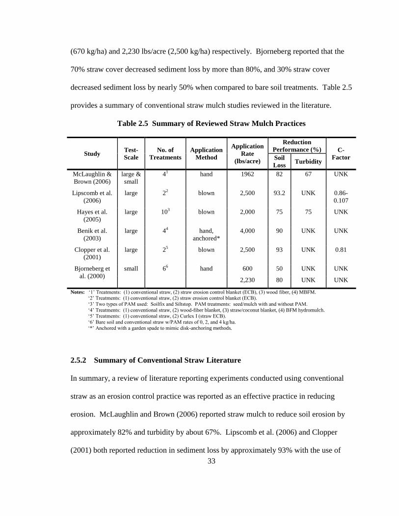
(670 kg/ha) and 2,230 lbs/acre (2,500 kg/ha) respectively. Bjorneberg reported that the
70% straw cover decreased sediment loss by more than 80%, and 30% straw cover
decreased sediment loss by nearly 50% when compared to bare soil treatments. Table 2.5
provides a summary of conventional straw mulch studies reviewed in the literature.
Table 2.5 Summary of Reviewed Straw Mulch Practices
Study Test-
Scale
No. of
Treatments
Application
Method
Application
Rate
(lbs/acre)
Reduction
Performance (%) C-
Factor Soil
Loss Turbidity
McLaughlin &
Brown (2006)
large &
small
41
hand 1962 82 67 UNK
Lipscomb et al.
(2006)
large 22
blown 2,500 93.2 UNK 0.86-
0.107
Hayes et al.
(2005)
large 103
blown 2,000 75 75 UNK
Benik et al.
(2003)
large 44
hand,
anchored*
4,000 90 UNK UNK
Clopper et al.
(2001)
large 25
blown 2,500 93 UNK 0.81
Bjorneberg et
al. (2000)
small 66
hand 600 50 UNK UNK
2,230 80 UNK UNK
Notes: ‗1‘ Treatments: (1) conventional straw, (2) straw erosion control blanket (ECB), (3) wood fiber, (4) MBFM. ‗2‘ Treatments: (1) conventional straw, (2) straw erosion control blanket (ECB).
‗3‘ Two types of PAM used: Soilfix and Siltstop. PAM treatments: seed/mulch with and without PAM.
‗4‘ Treatments: (1) conventional straw, (2) wood-fiber blanket, (3) straw/coconut blanket, (4) BFM hydromulch. ‗5‘ Treatments: (1) conventional straw, (2) Curlex I (straw ECB).
‗6‘ Bare soil and conventional straw w/PAM rates of 0, 2, and 4 kg/ha.
‗*‘ Anchored with a garden spade to mimic disk-anchoring methods.
2.5.2 Summary of Conventional Straw Literature
In summary, a review of literature reporting experiments conducted using conventional
straw as an erosion control practice was reported as an effective practice in reducing
erosion. McLaughlin and Brown (2006) reported straw mulch to reduce soil erosion by
approximately 82% and turbidity by about 67%. Lipscomb et al. (2006) and Clopper
(2001) both reported reduction in sediment loss by approximately 93% with the use of

34
blown straw as an erosion control practice. Hayes et al. (2005) also found similar results
to McLaughlin and Brown (2006), reporting a near 75% reduction in both soil loss and
turbidity. Lastly, Bjorneberg et al. (2000) found a reduction in sediment loss by
approximately 80% when a 2.4% slope is 70% covered by straw mulch. All of the
literature herein reported significant reductions in sediment loss when conventional straw
is properly applied to slopes.
2.5.3 Hydromulch Literature
Hydraulic applications of mulch to slopes, referred to herein as hydromulching, for the
purpose of erosion control, is a developing industry. However, a review of literature
indicate that only a limited number of hydromulch studies conducted (McLaughlin and
Brown, 2006; Holt et al., 2005; Benik et al., 2003; Landloch, 2002; Buxton et al., 1979),
which indicated a need for further testing of hydromulch practices to effectively evaluate
performance of hydromulch products used for erosion control.
McLaughlin and Brown (2006), conducted large- and intermediate-scale tests on four
ground cover practices, two of which were straw mulch and a mechanically bonded fiber
matrix (MBFM) hydromulch. The MBFM was applied using a commercial hydroseeder
at Profile Product‘s manufacturer specified rate of 3,000 lbs/acre (3,360 kg/ha). In this
comparative study of ground covers, it was reported that the ground covers reduced
runoff turbidity by a factor of 4 or greater when compared to bare soil. More specifically,
on the controlled, intermediate-scale tests, the MBFM reduced average turbidity by
approximately 85% and sediment loss by about 86%.

35
Holt et al. (2005) performed intermediate-scale tests on six hydromulch treatments using
2 ft (0.61 m) wide by 10 ft (3.05 m) long by 3 in (7.6 cm) deep trays with a sandy clay
loam. The soil was packed, leveled, and set at a 15.7 % slope, and the following six
hydromulches were applied by hand at 1,000 lbs/acre (1,120 kg/ha) and 2,000 lbs/acre
(2,240 kg/ha): wood hydromulch, paper hydromulch, cottonseed hulls hydromulch,
COBY hydromulch produced from stripper waste (COBY Red), COBY produced from
picker waste (COBY Yellow), and COBY produced from ground stripper waste (COBY
Green). COBY is a term used in Holt‘s report to represent a patented cotton by product
of cottonseed hulls (Hold and Laird, 2002). Holt‘s rainfall simulator produced a rainfall
intensity of 2.5 in/hr (6.35 cm/hr). The results for Holt‘s testing were reported using a
cover factor at 1,000 lbs/acre (1,120 kg/ha) and 2,000 lbs/acre (2,240 kg/ha), where
COBY Green, COBY Red, COBY Yellow, cottonseed hulls, paper, and wood
hydromulches yielded factors of approximately 0.20 and 0.32, 0.10 and 0.22, 0.20 and
0.22, 0.16 and 0.21, 0.42 and 0.68, and 0.65 and 0.81 respectively.
Landloch (2002) studied the performance of four hydromulch treatments using fifteen
plots that were 16.4 ft long by 4.9 ft wide (5 m long by 1.5 m wide) at a 25% slope on
alluvial black, cracking clay soil. Rainfall was simulated mimicking a 1:10 year storm
for 20 minutes at an intensity of 5.7 in/hr (145 mm/hr). The four hydromulches tested
were paper hydromulch, flax hydromulch, flax plus paper hydromulch, and sugar cane
hydromulch, applied at a rate of 893 lbs/acre (1,000 kg/ha), 2,232 lbs/acre (2,500 kg/ha),
2,900 lbs/acre (3,250 kg/ha), and 4,464 lbs/acre (5,000 kg/ha) respectively. Results

36
reported in a cover factor showed paper, flax, flax plus paper, and sugar cane
hydromulches to have cover factors of 0.204, 0.149, 0.044, and 0.037 respectively.
Benik et al. (2003) developed a study comparing the effectiveness of five treatments,
including Soil Guard® which is a bonded fiber matrix (BFM) that has been on the
hydromulch market since 1993. The experimental setup of this experiment is referenced
in Section 2.5.1. In this experiment, the BFM was applied at a minimum rate of 3,000
lbs/acre (3,360 kg/ha). Manufacture specifications require a 24 hour drying period;
however this procedure was not reported in Benik‘s research. According to results, the
Soil Guard® BFM reduced average sediment yield by approximately 94%. Turbidity
was not reported in this research effort.
The last hydromulch study examined was an extensive evaluation of selective erosion
control techniques, completed by Buxton and Caruccio in 1979 of the University of South
Carolina, in collaboration with the USEPA. For this research effort, 19 soil stabilizing
and erosion control treatments were tested at specially prepared field, four of which were
hydromulches without tackifiers. The plot sizes used were approximately 5 ft (1.5 m)
wide by 10 ft (3 m) long at a 12 to 15% slope, and the soil tested was a Herndon silt
loam. The testing relied on natural rainfall, and in central South Carolina, which is where
testing was conducted. A 3.5 inch (8.9 cm) 24-hour rainfall event with a recurrence
interval of 2 years was recorded. The four hydromulches tested were Conwed wood fiber
mulch, Superior wood fiber mulch, Silva wood fiber mulch, and Pulch; each hydromulch
was applied at a rate of 1,200 lbs/acre (1,344 kg/ha). In this study, effectiveness of the

37
hydromulches were measured using a vegetative maintenance and erosion control (VM)
value, which in 1979 was a new parameter in the Universal Soil Loss Equation (USLE),
and represented total loss ration expressed as a decimal. These values ranged from 0.0 to
1.0, where a value of 1.0 means the ESC practice had no effect in reducing erosion. The
VM values for Buxton and Cauccio‘s (1979) report were 0.235, 0.266, 0.655, and 0.280
for Conwed wood fiber mulch, Silva wood fiber mulch, Superior wood fiber mulch, and
Pulch, respectively. If these values were translated to measure erosion control
performance in percent efficiency, Conwed, Silva, Superior, and Pulch hydromulches
would have respective values of 76.5%, 73.4%, 34.5%, and 72%, respectively.
Table 2.6 provides a summary of hydromulch studies reviewed in the literature.

38
Table 2.6 Summary of Reviewed Hydromulch Practices
Study Type of
Hydromulch Test-Scale Slope
Application Rate
(lbs/acre)
Reduction Performance (%) C-Factor
Soil Loss Turbidity
McLaughlin &
Brown (2006)
MBFM1
large &
intermediate
10% and 20% 3,000 86 85 UNK
Holt et al. (2005)2 Wood
Paper
Cottonseed hulls
COLBY red
COLBY yellow
COLBY green
intermediate 15.7% 1,000 and 2,000 35 and 19
58 and 32
84 and 79
90 and 88
80 and 88
80 and 68
UNK
UNK
UNK
UNK
UNK
UNK
0.65 and 0.81
0.42 and 0.68
0.16 and 0.21
0.10 and 0.22
0.20 and 0.22
0.20 and 0.32
Benik et al. (2003) BFM3
large 35% 3,000 94 UNK UNK
Landloch (2002) Paper
Flax
Flax plus paper
Sugar Cane
large 25% 892
2232
2900
4464
80
85
96
96
UNK
UNK
UNK
UNK
0.204
0.149
0.044
0.037
Buxton and
Caruccio (1979)4
Conwed*
Superior*
Silva*
Pulch*
large 12% to 15% 1,200 77
73
35
72
UNK
UNK
UNK
UNK
0.235
0.266
0.265
0.280
Notes: ‗1‘ Mechanically Bonded Fiber Matrix.
‗2‘ Hydromulches were applied by hand. ‗3‘ Bonded Fiber Matrix.
‗4‘ A Modified Universal Soil Loss Equation (USLE) was used to calculate C-factors.
‗*‘ All are wood-fiber hydromulches.

39
2.5.4 Summary of Hydromulch Literature
In summary, although the literature data on hydromulch is limited, the research results
show significant reductions in soil loss and turbidity. McLaughlin and Brown (2006)
conducted intermediate-scale tests to determine the performance of a MBFM, and
concluded an 85% reduction in turbidity and 86% reduction in soil loss when compared
to bare soil conditions. Similarly, Benik et al. (2003) reported a near 94% reduction in
sediment loss while testing the performance of a BFM on a large-scale. Holt et al. (2005)
and Landloch (2002) tested the performance of several wood and paper hydromulches,
and Landloch added cottonseed hull hydromulches to his effort; amongst these tests,
sediment reduction results were reported as low as 19% to as high as 96%. Lastly, during
a time when hydromulching was less common, extensive intermediate-scale testing of
four hydromulches containing no tackifiers by Buxton and Carrucio (1979) yielded
results on several fiber-mulch products to have erosion control capabilities of nearly
76%. Although the experimental designs and procedures varied, it was concluded by
each researcher that when hydromulch is applied at manufacturer specifications, it is a
very effective erosion control practice.
2.6 Literature Review Summary
Runoff from construction sites has been recorded to be the largest contributor of non-
point source pollution in the United States. Therefore, over the past century, the USEPA
has been actively developing guidelines to control construction site runoff.

40
In this chapter, a history of USEPA ELG and regulations were discussed as well as
guidelines that have been established within the past year. These federal guidelines are
vital knowledge for the research effort herein because they set specific parameters for
construction site runoff. The federal government, however, has given the state of
Alabama the authority to create stricter ELGs and regulations for construction site runoff,
as discussed previously.
With the implementation of stricter ELGs and regulations for construction sites over the
past decade, there has been an increased desire in the state of Alabama from contractors
and the ALDOT to obtain knowledge of products that provide the most effective ESC.
One of the oldest, cheapest, and most prevalent measures of erosion control is
conventional straw mulch. Researchers‘ results within reports on the use and
effectiveness of conventional straw were widely different. However, overall, it is
accepted that when conventional straw is applied properly and uniformly to slopes that
are less than a 33% grades, it is very effective erosion control practice. When slopes are
equal to or steeper than 33%, to avoid wind erosion or runoff washing away the
lightweight straw, the straw must be anchored to the ground. As discussed, the two most
common forms are ‗crimping‘ the straw to the ground with a machine, or applying a
tackifier to create a bond between the straw and the ground.
The hydraulic application of mulch (a.k.a. hydromulching) is a relatively new ESC
practice, and due to advancements in technologies has become a widely use practice in
the industry. Hydromulching has enabled contractors to apply mulches containing

41
tackifiers and bonding agents to steep slopes efficiently and effectively. Although
limited, previous studies reviewed commonly report hydromulching to be an effective
erosion control measure, due the inconsistencies of reported results, it is difficult to
properly determine the effectiveness of hydromulches. Thus, further experiments need to
be conducted on hydromulches to gain a more comprehensive understanding of
hydromulch performance.
42
Chapter 3 Intermediate-Scale Test Methods and Procedures
3.
3.1 Introduction
Research previously conducted by Shoemaker et al. (2009) shows several different
experimental methods, procedures, and designs to test the performance of ESC practices.
To create comparable data, Shoemaker‘s (2009) intermediate-scale test methods and
procedures where used as a guideline for this research effort. However, several
modifications to his designs were made, which include: (1) a replicate design and
construction of new intermediate-scale test plots, with a new flume design that was used
as the collection device, (2) attaining and testing new soil from a local stockpile and
conducting soil and compaction analyses, and (3) newly developed hydromulch
experimental procedures.
3.2 Intermediate-Scale Testing
The validity of this research effort relies heavily on the amount of reproducible data that
is collected during experiments which can be used for comparative analyses to evaluate
ESC practice performance and effectiveness. Thus, when designing the experimental
procedures, it was pertinent that the size of the test plots were constructed with the
purpose of testing ESC practices with ease, speed, accuracy, and mobility throughout the
experiment. Thus, if all procedural expectations were satisfied, replications of
experiments could be performed to develop adequate data sets for comparative analyses.

43
The focus of this chapter is to discuss the facility, equipment, modifications made to
previous experimental design (Shoemaker, 2009), setup, and testing procedure.
3.2.1 Intermediate-Scale Test Facility
A 20 ft by 30 ft by 15 ft (6.1 m by 9.1 m by 4.6 m) building, consisting of two drum roll
up doors at opposite ends of the structure located at the National Center for Asphalt
Technology (NCAT), as depicted in Figure 3.1(a) was used to perform all intermediate-
scale experiments. As shown in Figure 3.2, the interior of the building is equipped with
two water faucets located at the northeast and southeast corners of the building that are
supplied by a nearby underground well, indoor lighting, electrical outlets, and WI-FI
internet access. Southwest of the building, jersey barriers were aligned to established
areas to stockpile soil used during experiments and dispose of post-experiment soil,
shown in Figure 3.1(b). A tarp covers the soil to be tested to ensure consistent moisture
content and to prevent contamination of the stockpile. Gravel surrounds the building as
an erosion control measure and for heavy equipment mobility.

44
(a) Testing Facility Building (b) Storage bins
Figure 3.1 Test Facility Exterior.
(a) East Side of Building
(b) West Side of Building
Figure 3.2 Test Facility Interior.

45
3.2.2 Hydroseeder
The hydroseeder used to apply the hydromulch to all test plots was a Turf Maker® 380 as
shown in Figure 3.3(a), 3.3(b), and 3.3(c). This hydroseeder has a 380 gallon capacity to
hold hydromulch and water mixtures. The hydroseeder has a mechanical agitator and a
positive displacement pump that are powered by a Briggs and Stratton Intex 1450 engine.
(a) TurfMaker® 380
(b) Mechanical Agitator (c) Engine and Discharge Pump
Figure 3.3 Illustrations of TurfMaker® 380 and Various Features.

46
3.3 Experimental Design
The experimental design, adopted from Shoemaker‘s (2009) intermediate-scale research
efforts is specific to compacted highway embankments on a 3H:1V slope, which are
subject to a simulated 2-yr, 24-hr rainfall event.
3.3.1 Intermediate-Scale Test Plots
Test plots constructed for this research effort were replicas of Shoemaker‘s (2009) test
plots with the exception of the runoff collection device. Each test plot is 2 ft in width by
4 ft in length (0.6 m by1.2 m) by 3.5 inches (7.62 cm) in depth. In previous efforts
(Shoemaker 2009), a gutter device was designed and constructed to collect runoff from
test plots. The gutter device shown in Figure 3.4(a), collected soil and runoff from the
test plots, however the device had to be constantly monitored to ensure soil did not reside
within the gutter itself, ultimately affecting quantification of soil loss over time.
Therefore, when the new test plots were constructed, an aluminum flume was designed
and constructed to ensure consistent collection of runoff, as depicted in Figure 3.4(b).
(a) Shoemaker (2009) Gutter Collection Device (b) Flume Collection Device
Figure 3.4 Comparison of Collection Devices.

47
The abovementioned intermediate-scale test plots were constructed for the purpose of
simultaneous experimentation. Each plot was constructed with pressurized, treated
timber. The base of the plot was cut out of a ½ inch (1.27 cm) piece of plywood and the
perimeters of the box plot were built with two-by-fours. After construction, the box plots
were primed, painted, and the crevices were caulked to increase the durability of the box
plots and to minimize water seepage. Also, galvanized handles were screwed to the side
of the plots to aid in mobilization. With the intention of observing and collecting any
possible infiltration through the soil, a metal strip with 3/8 inch (9.525 mm) holes and a
polyvinyl chloride (PVC) pipe cut in half was installed at the base of the test plot, shown
in Figure 3.4(b). The infiltration holes were deemed unnecessary after several tests in
which no infiltration was observed or collected. The flumes were designed and
constructed with the help of Auburn University‘s Machine Shop, and fastened securely to
the end of the box plots with four, 1½ inch (38.1 mm) galvanized exterior screws.
In Shoemaker‘s (2009) previous research efforts, a total of 2 inches (5.08 cm) of
compacted soil was placed in each plot, one inch layer at a time, which allowed for
approximately 1½ inches (3.81 cm) difference in height between the top of the soil and
the top of the plot perimeter. After discussions with ALDOT, it was determined that by
compacting 1 inch (2.54 cm) layers at a time inherently over compacted each soil layer.
Therefore a decision was made to compact 3 inches (7.62 cm) of soil, in one layer,
leveling the top of the soil with the box plot perimeter. After the first test run, it was
evident two sideboards needed to be constructed out of flashing and two by fours to
direct runoff from the compacted box plots to the flume outflow, illustrated in Figure 3.5.

48
Figure 3.5 Sideboards Installed on Test Plots.
Mobility of the box plots was a crucial factor in the experimental design because it
allowed the researcher to have a rapid setup, as well as a quick cleanup post-experiment.
The setup shown in Figure 3.6 illustrates that each box plot was positioned on a 3H:1V
slope supported by sawhorses and cinder blocks.
Figure 3.6 3H:1V Slope using Cinderblocks and Saw Horses.
3
1
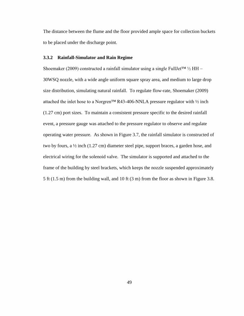
49
The distance between the flume and the floor provided ample space for collection buckets
to be placed under the discharge point.
3.3.2 Rainfall-Simulator and Rain Regime
Shoemaker (2009) constructed a rainfall simulator using a single FullJet™ ½ HH –
30WSQ nozzle, with a wide angle uniform square spray area, and medium to large drop
size distribution, simulating natural rainfall. To regulate flow-rate, Shoemaker (2009)
attached the inlet hose to a Norgren™ R43-406-NNLA pressure regulator with ½ inch
(1.27 cm) port sizes. To maintain a consistent pressure specific to the desired rainfall
event, a pressure gauge was attached to the pressure regulator to observe and regulate
operating water pressure. As shown in Figure 3.7, the rainfall simulator is constructed of
two by fours, a ½ inch (1.27 cm) diameter steel pipe, support braces, a garden hose, and
electrical wiring for the solenoid valve. The simulator is supported and attached to the
frame of the building by steel brackets, which keeps the nozzle suspended approximately
5 ft (1.5 m) from the building wall, and 10 ft (3 m) from the floor as shown in Figure 3.8.

50
Figure 3.7 Illustration of Rainfall Simulator.
Figure 3.8 Illustration of Simulator Relative to Plots.

51
Shoemaker‘s research efforts also included an extensive calibration and validation of the
rainfall simulator to determine and analyze rainfall amount and uniformity (2009). The
Christiansen Uniformity Coefficient (ASAE Standards, 2000) was used to quantify the
uniformity of the rainfall distribution over the 8 ft by 8 ft (2.4 m by 2.4 m) spray area the
nozzle covers. Shoemaker was able to quantify that the rainfall distribution uniformity
ranged from 83% to 88%; generally, in the center 4 ft by 4 ft (1.2 m by 1.2 m) area.
Christiansen Uniformity Coefficients of 80% or higher are deemed to be uniform.
After calibrating the rainfall simulator, a proper rainfall regime needed to be designed to
be representative of a 2-yr, 24-hr rainfall event. Previous literature reviewed showed
varying rainfall regimes due to various intensity-duration-frequency (IDF) curves and
locations. ALDOT stormwater inspection guidelines state that an inspection of any ESC
practice is required within 72 hours of a ‗qualifying event‘. A qualifying event is any
rainfall that accumulates 0.75 inches (1.9 cm) of rain within a 24 hour period (ALDOT
2004). Therefore, 0.75 inches (1.9 cm) was used as a baseline to select the design storm
rainfall regime. From Shoemaker‘s calibration process, he was able to determine that an
operating pressure of 10 psi (69 kPa) is capable of generating an intensity of 4.39 in/hr
(11.15 cm/hr) (2009). From this intensity, a rainfall duration of 15 minutes produces
approximately 1.1 inches (2.8 cm) of rain, which is above the 0.75 inch (1.9 cm) baseline.
In addition to ALDOT‘s inspection guidelines, Shoemaker used an IDF curve for
Auburn, Alabama. Using ALDOT‘s guidelines, the IDF curve, and Shoemaker‘s rainfall
calibration, it was determined that a 2-year, 24-hour rain event for Auburn, Alabama
would produce a cumulative rainfall amount of 4.39 in/hr (11.2 cm/hr) intensity. To
52
simulate a 2-yr, 24-hr design storm, the rainfall simulator which produces 1.1 inches (2.8
cm) over a 15 minute period would need to consist of 4, 15 minute rainfall events, lasting
1 hour. The rain regime used by Shoemaker (2009) was adopted for this research effort
consisting of 4, 15 minute events, representative of a 2-yr, 24-hr event with a total rainfall
amount of 4.4 inches (10.9 cm).
3.4 Experimental Procedures Pre-Condition Application
A large majority of the experimental procedures and methods were adopted from
Shoemaker (2009), however there were several modifications made to the experimental
procedures due to a change in the ESC practices tested. Modifications included test
protocol and procedures pertaining to application of the hydromulch product. Also, a soil
and compaction analysis were conducted on a new stockpile of soil.
3.4.1 Soil Analysis
Soil for the research effort herein was provided by a local grading contractor from a
construction site near the NCAT test track in Opelika, Alabama (32°33‘5‖ N, 85°20‘28‖
W). A soil analysis was conducted by the Auburn University Soil Testing Laboratory to
determine the soil composition, shown in Table 3.1 below.
Table 3.1 Percent Composition and Classification of Experimental Soil
% Sand % Silt % Clay Classification
67.5 2.5 30 Sandy Clay Loam
The soil analysis yielded nearly 2/3 sand and 1/3 clay composition, and less than 3% silt
content which classified the soil as a sandy, clay loam.

53
3.4.2 Compaction Analysis
After classifying the soil, a compaction test was conducted. ALDOT specifies in its
Standard Specifications for Highway Construction (2008) that on a typical highway
embankment, slopes should be compacted to 95% compaction. This requirement was
adopted by Shoemaker (2009) who used hand tamps dropped on the box plots to achieve
optimum compaction.
To determine the number of drops required to compact the soil, two compaction tests
were completed. The first soil compaction test was to determine the optimum moisture
content (OMC) of the soil. This was completed using a modified Proctor test, as
specified in American Society for Testing and Materials (ASTM) D1557. The modified
Proctor test enabled researchers to develop a Proctor curve representing the moisture
content of the soil versus the dry unit weight of the soil, as shown in Figure 3.9.
Figure 3.9 Proctor Curve for Experimental Soil.
100
103
106
109
112
0% 5% 10% 15% 20% 25% 30%
Dry
Un
it W
eig
ht (p
cf)
Moisture Content (%)
Data Points Maximum Density Point Calculated Curve Points
95% Compaction

54
The Proctor curve shown in Figure 3.9 illustrates four determined moisture contents to
achieve a specific dry unit weight for the tested soil. An optimum moisture content
(OMC) was determined to be 111 pcf (1762 kg/m3) at 14% moisture content (MC) by
locating the maximum dry unit weight on the Proctor curve. The dotted line shown in
Figure 3.9 represents the minimum dry unit weight of 105 pcf (1682 kg/m3) required to
reach ALDOT‘s specified 95% compaction rate over a range of moisture content (5% to
23%).
The second compaction test, also adopted from Shoemaker was created to test the number
of hand tamps required to achieve 95% compaction. Shoemaker designed and
constructed a 1ft by 1ft (30.5 cm by 30.5 cm) wood box specifically sized to fit the hand
tamps, shown in Figure 3.10.
Figure 3.10 Mold used to Determine Required Compaction Rate with Hand-Tamp.

55
The molded boxes were designed to allow the hand tamps to fit inside the perimeter. The
hand-tamps measured 10 in. by 10 in. (25.4 cm by 25.4 cm), and the mold measured 1 ft
by 1 ft (30.5 cm by 30.5 cm). The purpose of this compaction test was to drop the hand
tamp a specified number of times upon a known volume of compacted soil to determine a
corresponding unit weight. Soil with a MC of approximately 14% was loaded into the 1
ft by 1 ft by 2 inch (30.5 cm by 30.5 cm by 5.1 cm) box and a hand tamp was dropped
approximately 12 inches (30.5 cm) from the soil surface in a series of 5 sets: 10 drops,
20 drops, 30 drops, 50 drops, and 60 drops. After each set of drops, the mold was
screeded to a height of 1 inch, the known volume of soil was weighed, and a measured
compacted dry unit weight was calculated, and plotted on a graph, shown in Figure 3.11.
Figure 3.11 Compaction of Soil Using Hand Tamps.
y = 38.08x0.2348
R² = 0.997
50
60
70
80
90
100
110
0 10 20 30 40 50 60 70
Mea
sure
d C
om
pa
cted
Dry
Un
it W
eig
ht (p
cf)
Number of Drops

56
Figure 3.11 is a representation of number of drops with a hand tamp in correlation with
its corresponding measured compacted dry unit weight. When compacted, soil will
approach a point where it has reached maximum compaction, preventing any further
compaction. A regression line and power function was applied to the points on the plot
to illustrate the point at which soil can no longer be further compacted. When the
regression line levels off, the soil has reached maximum compaction, regardless of
energy applied by the hand tamps. Using the power function, the specified number of
drops required to reach optimum compaction was calculated, shown in Table 3.2.
Table 3.2 Calculated Dry Unit Weight (pcf)
and Required Number of Drops
Number of Drops Dry Unit Weight (pcf)
10 65.4
20 76.9
30 84.6
40 90.5
50 95.4
60 99.6
70 103.3
80 106.5
90 109.5
100 112.3
To obtain a minimum of 95% compaction, a minimum dry unit weight of 105 pcf (1,682
kg/m3) was required, which corresponded to approximately 80 hand-tamps.
3.4.3 Hydromulch Product Selection
Stricter regulations by the USEPA regarding ESC on construction sites has established a
need to determine practices that can be installed easily, cost efficiently, and comply with
EPA stormwater runoff regulations. In the summer of 2009, ALDOT and the Department
of Civil Engineering at Auburn University showed a joint interest in testing the

57
performance of mulches that are hydraulically applied, referred to herein as
hydromulches, to 3H:1V fill slopes as an innovative erosion control practice. Although
mulching is not a new erosion control practice, advanced technologies in pumps and
hydroseeders have made hydraulic application of mulch a highly prevalent procedure of
application. Hydromulches have been tested on a large-scale (McLaughlin and Brown,
2006; Holt et al., 2005; Benik et al., 2003; Landloch, 2002; Buxton and Caruccio, 2000),
however, further investigation of the performance of hydromulch products on an
intermediate-scale is needed. Therefore, ALDOT assigned a number of hydromulches
that are ubiquitous in the erosion control industry to be tested and evaluated. Table 3.3
below shows a list of four hydromulches and their corresponding mulch classification
that were tested in this research effort.
Table 3.3 Assigned Hydromulch and Classification
Type of Hydromulch Classification
GeoSkin Hydraulic Mulch Product, w/Tackifier
HydraCX2
Bonded Fiber Matrix (BFM)
Excel Fibermulch II Hydraulic Mulch Product, w/o Tackifier
HydroStraw BFM Bonded Fiber Matrix (BFM)
To create a baseline comparison, bare soil control was tested, as well as two conventional
straw mulch practices: (1) that has been crimped and (2) that has been applied with a
tackifier. Although bare soil was the only condition used as a basis of analyzing erosion
control performance, conventional straw, crimped or tackified, was tested and evaluated
as a second baseline comparison due to its cost efficiency and that is it a predominantly
used mulch in the industry.

58
3.4.4 Experimental Organization
Figure 3.12 is a flowchart showing the seven conditions tested: (1) one bare soil control;
(2) conventional straw, crimped; (3) conventional straw, tackified; (4) GeoSkin®; (5)
HydraCX2®; (6) Excel® Fibermulch II; and (7) HydroStraw® BFM. The bare soil
condition serves as the control, and conventional straw conditions were developed as a
baseline condition for comparison of traditional mulching practices to newer hydromulch
technologies currently being used in the industry. The experimental setup was organized
to allow two full experiments, consisting of 4 total plots, to be run on each condition. An
experiment, as illustrated in Figure 3.12, consists of two test plots centered beneath the
rainfall simulator to experience the design rainfall event and total rainfall amount
discussed in Section 3.3.2. As previously discussed, and shown in the flowchart, four
‗tests‘ were simulated within a single experiment, with a 15 minute break between storm
events to allow for data collection.

59
Figure 3.12 Flowchart of Experimental Organization.
Control – Bare Soil
Left Plot – 4 Tests
Right Plot – 4 Tests
Left PlotTest 1
15 min event
15 min break
Test 2
15 min event
15 min break
Test 3
15 min event
15 min break
Test 4
15 min event
Right PlotTest 1
15 min event
15 min break
Test 2
15 min event
15 min break
Test 3
15 min event
15 min break
Test 4
15 min event
Experiment 1
Treatment 1 – Conventional
Straw Mulch, crimped
CONDITION(s) EXPERIMENT(s) TEST(s)
Experiment 2
Treatment 2 – Conventional
Straw Mulch w/Tackifier
Treatment 3 – GeoSkin
Treatment 4– HydraCX2
Treatment 5 – Excel
Fibermulch II
Treatment 6 – HydroStraw
Mulch

60
3.4.5 Test Plot Preparation
The test plot preparation used for this research was modified from Shoemaker‘s (2009)
research. Shoemaker (2009) developed a five step process for his test plot preparation;
however due the different products tested, the test preparations were changed slightly.
For this research effort, test plot preparation is divided into two sections: (1) test plot
preparation prior to condition application, and (2) condition application test protocols and
procedures.
3.4.5.1 Test Plot Preparation Prior to Condition Application
Section 3.4.2 described the method used to determine the number of drops required by a
hand tamp to reach optimum compaction, and the MC necessary to achieve the required
compaction. To assure the MC of the soil was within the limits of the minimum dry unit
weight of 105 pcf (1,682 kg/m3), a small sample of the stockpile was dried using a double
hotplate electric stove provided by the NCAT facility. After determining the MC of the
soil, if the stockpile is above 23% it is left to dry until within the minimum MC for the
acceptable 95% compaction. If the soil happened to be too dry, water was added until the
proper MC was obtained.
In Shoemaker‘s research effort, after the moisture content was determined, two, 5 gallon
buckets of soil were loaded into a wheelbarrow, added the proper amount of water, if
necessary and compacted a one inch layer of soil. This step was repeated to obtain two
compacted 1 inch layers of soil (2009). In this research effort, we used one, 3 inch (7.62
cm) layer of compacted soil and a scoured surface to simulate a more realistic highway
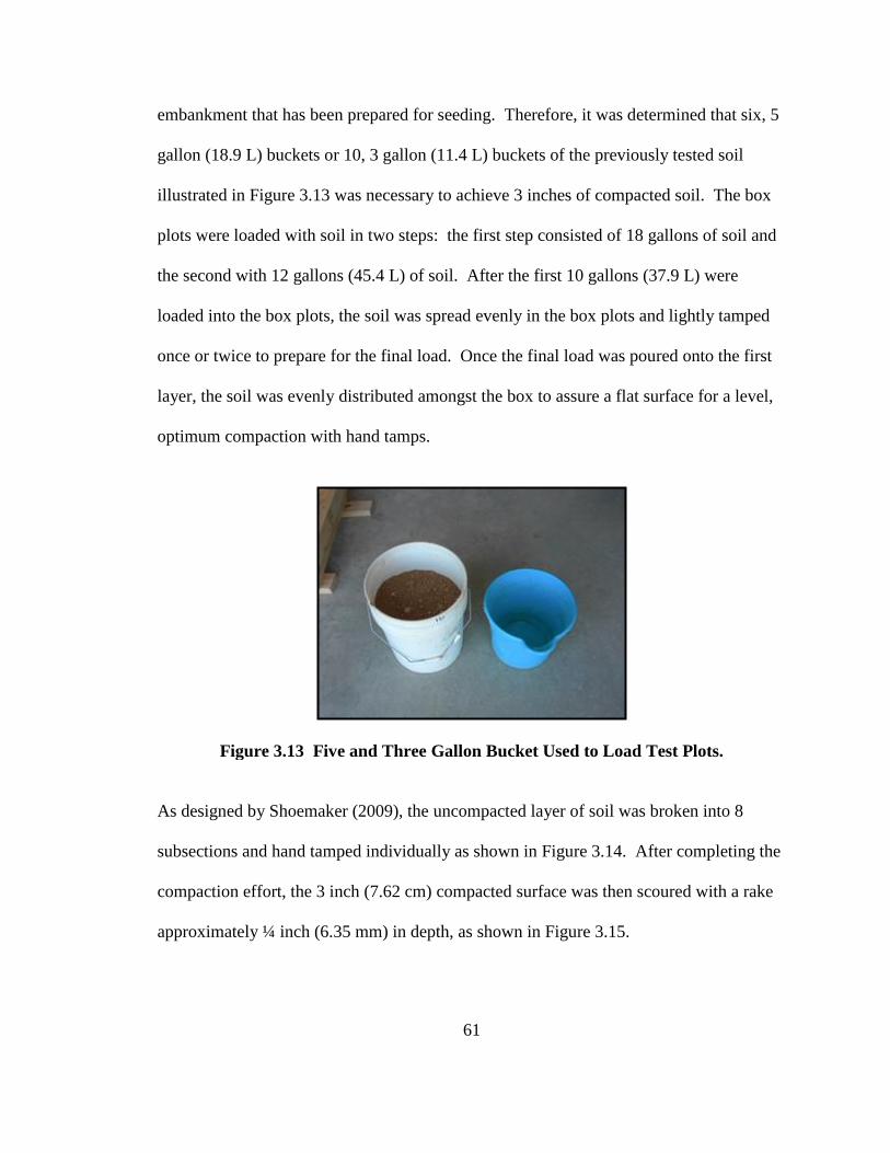
61
embankment that has been prepared for seeding. Therefore, it was determined that six, 5
gallon (18.9 L) buckets or 10, 3 gallon (11.4 L) buckets of the previously tested soil
illustrated in Figure 3.13 was necessary to achieve 3 inches of compacted soil. The box
plots were loaded with soil in two steps: the first step consisted of 18 gallons of soil and
the second with 12 gallons (45.4 L) of soil. After the first 10 gallons (37.9 L) were
loaded into the box plots, the soil was spread evenly in the box plots and lightly tamped
once or twice to prepare for the final load. Once the final load was poured onto the first
layer, the soil was evenly distributed amongst the box to assure a flat surface for a level,
optimum compaction with hand tamps.
Figure 3.13 Five and Three Gallon Bucket Used to Load Test Plots.
As designed by Shoemaker (2009), the uncompacted layer of soil was broken into 8
subsections and hand tamped individually as shown in Figure 3.14. After completing the
compaction effort, the 3 inch (7.62 cm) compacted surface was then scoured with a rake
approximately ¼ inch (6.35 mm) in depth, as shown in Figure 3.15.

62
Figure 3.14 8 Sections to Compact Approximately 80 Times.
Figure 3.15 Uniform Tilling of Surface Approximately ¼ inch in Depth.
Although this research effort does not test longevity or seedling germination, the purpose
of scouring the surface of the compacted soil was to simulate a realistic ALDOT highway
embankment, which generally includes tilling for spreading seed and fertilizer. Once the

63
tilling effort was completed, the box plots were ready for condition applications (i.e.,
hydromulch or conventional straw).
3.5 Condition Application Experimental Procedures
Consistent test methods and procedures, while also ensuring that this research adheres to
the manufacturers‘ specification for proper application rates on a 3H:1V slope, are vital
to the integrity of the research. Thus, each condition was evaluated separately and an
application process was developed specifically for each test.
A bare soil test was initially chosen as the control condition for this testing, however
ALDOT became interested in testing an application of conventional straw mulch that was
either crimped or sprayed with a tackifier. The first section will entail the application
process of conventional straw applied at ALDOT specified 4,000 lbs/acre (4,480 kg/ha)
that has been crimped or sprayed with a tackifier.
Different hydromulch products are comprised of diverse materials, as explained in the
‗literature review‘ portion of this research; therefore different application rates are
required, dependent upon steepness of slope. For a 3H:1V slope, the hydromulch
application rates ranged from 2,000 lbs/acre to 3,500 lbs/acre (2,240 to 3,920 kg/ha). The
section following the conventional straw conditions‘ experimental procedures will report
the test protocols and procedures for the following hydromulch conditions: (1)
GeoSkin®; (2) HydraCX2®; (3) Excel® Fibermulch II; and (4)HydroStraw® BFM.

64
3.5.1 Conventional Straw, Crimped or with Tackifier Test Protocol
According to ALDOT‘s Standard Specifications for Highway Construction (2008),
conventional straw or hay that has been crimped and is placed on a 3H:1V or flatter slope
is considered a ‗Class A, Type 1‘ mulch. ‗Class A, Type 2‘ mulch is described as hay
mulch or conventional straw that uses an adhesive or tackifier. This section will describe
the necessary steps and test procedures required to produce an intermediate-scale test for
conventional straw crimped or tackified.
3.5.1.1 Conventional Straw, Crimped Test Protocol and Procedures
Conventional straw‘s typical form of application is mechanically, using a machine to
chop and blow the straw onto the slope to 75% or greater coverage, as shown in Figure
3.16, or it can be laboriously spread by hand.
Figure 3.16 Mechanically Blown Straw. (Source: http://www.clintontractor.net)

65
After the straw is spread, for slopes 3H:1V or flatter, the straw is typically crimped or
embedded into the soil by a mulch crimper to reduce the chance of the straw being blown
away by wind or moved due to excess runoff volumes. ALDOT (2008) requires the
crimper to be a roller type device equipped with flat, uncapped, dull edge disks with a
minimum width of ¼ inch (6 mm) and placed a maximum of 2 inches (5.1 cm) apart
along the axle or shaft, as shown in Figure 3.17.
Figure 3.17 Mulch Crimper. (Source: http://www.proseriesproducts.com/procrimper.htm)
ALDOT also specifies that the diameter shall be large enough to prevent the axle or shaft
from dragging or in any way disturbing the mulch or soil (2008). Crimpers should be
designed to apply enough force to embed the straw approximately 2 inches (50 mm) into
the soil (ALDOT, 2008).

66
Typically, conventional straw blowers and crimpers are used for application on large
areas or acres of land. Therefore, modifications to typical application of straw were
necessary for the intermediate-scale plots. The first modification made was converting
ALDOT‘s specified application rate of 4,000 lbs/acre (4,480 kg/ha) to the 2 ft x 4 ft (0.6
m by 1.2 m) test plot, which was equivalent to 333 grams/plot (0.333 kg/plot). Depicted
in Figure 3.18(a), (b), and (c) below, the proper amount of dry, conventional straw was
weighed and evenly applied by hand to the compacted and tilled test plot.
(a) Weighing Straw Prior to App.
(4,000 lbs/acre≈333 grams/plot)
(b) Application of Straw on Test Plots
(Minimum 70% cover)
(c) Plots after 4000 lbs/acre (333 grams/plot ) Application and 70% Cover
Figure 3.18 Weighing and Applying Conventional Straw.

67
After proper application of the conventional straw, the next task was to crimp the
conventional straw into the soil. A typical mulch crimper weighs several thousand
pounds; therefore an intermediate-scale crimper was designed. To simulate a crimping
wheel, a prototype was constructed from the basic performance of a wheel as it rolls over
the soil; the thought process of the design is shown in Figure 3.19.
Figure 3.19 Intermediate-Scale Mulch Crimper Design and Construction Process.
The crimper constructed above is 2 ft (0.6 m) in length by 3.5 inches (5.1 cm) in height,
and ¼ inch thick, which meets ALDOT specifications for a straw crimper. After
constructing the intermediate-scale crimper, the next task was to crimp the conventional
straw into the soil. Using a rubber mallet, the wooden crimper was positioned
horizontally along the box plot and pounded uniformly into the soil until it was
approximately 1 inch (25.4 mm) deep, as shown below in Figure 3.20.

68
Figure 3.20 Crimping Straw.
The conventional straw was crimped every two inches, as specified by ALDOT (2008).
Experimental testing was commenced after each test plot was completely crimped.
3.5.1.2 Conventional Straw, with Tackifier
ALDOT (2008) specifies ‗Class A, Type 2‘ mulching to be used on slopes steeper than
3H:1V, referred to herein as conventional straw with a tackifier. The type of tackifier
tested in this research effort was Hytac II which is manufactured by Easy Lawn, Inc.,
mixed at a rate of 52.8 oz (1,497 grams) per 600 to 700 gallons (2,270 to 2,650 liters),
and 1.1 oz/1,000 ft2;(31 grams/cm
2) this converts to approximately 0.088 to
0.075oz/gallon (0.66 to 0.56 grams/L), and 0.0088 oz/plot/0.1 gallons (¼
gram/plot/0.0.38 L). Test procedures for this section are identical to procedures outlined
in Section 3.5.1; however, the tackifier replaced the crimping method. To properly apply
the tackifier to the conventional straw, it was added to a Maruyama MS074 backpack

69
sprayer with a built in agitator. Specifications for the backpack sprayer are in Appendix
C. To avoid clogging of the backpack sprayer, the tackifier was added slowly to the tank.
Illustrated in Figure 3.21(a) and (b), the tackifier contained a blue dye for application
purposes.
(a) Hytac II (b) 0.5 grams of Hytac (applicatin rate for both test plots)
Figure 3.21 Hytac II—Tackifier for Convetional Straw.
After approximately 20 minutes of mixing, the tackifier was equally applied to both plots,
as shown in Figure 3.22 (a) and (b).
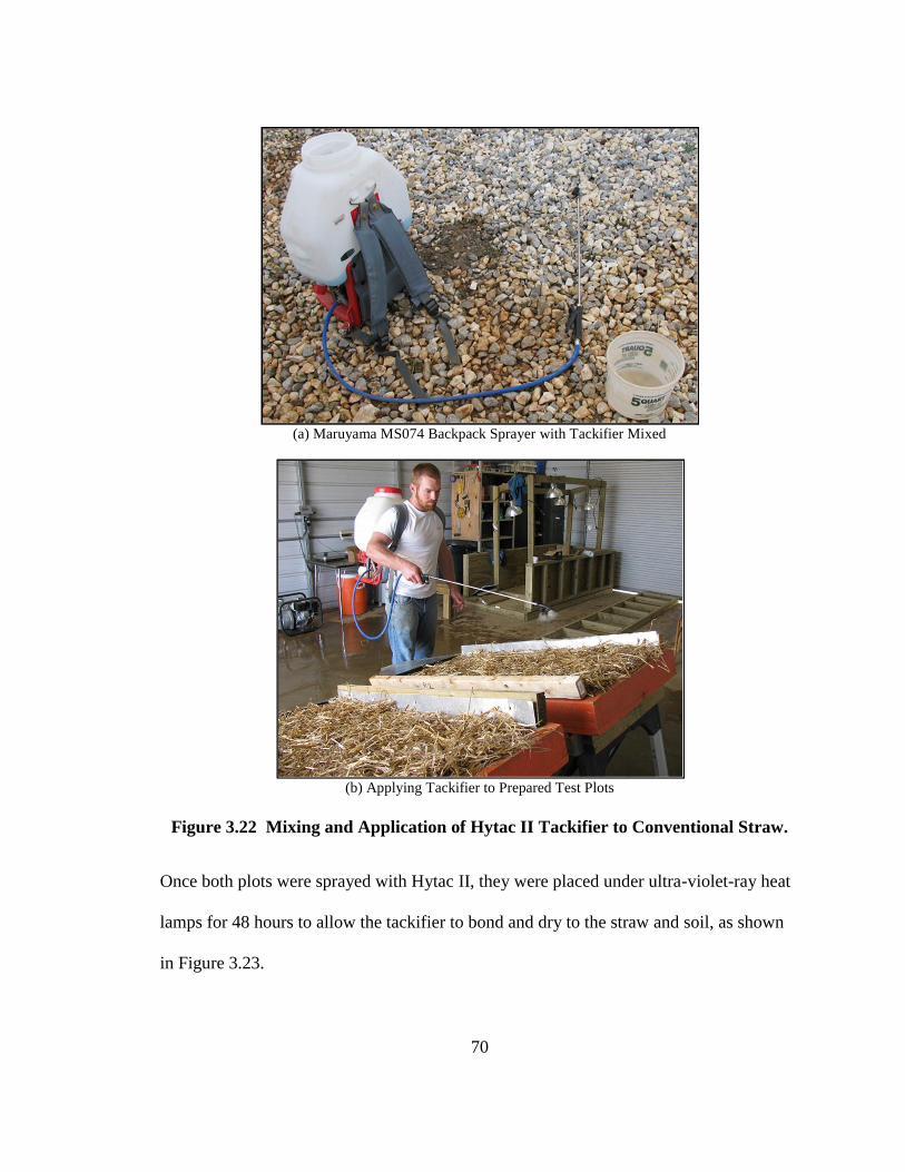
70
(a) Maruyama MS074 Backpack Sprayer with Tackifier Mixed
(b) Applying Tackifier to Prepared Test Plots
Figure 3.22 Mixing and Application of Hytac II Tackifier to Conventional Straw.
Once both plots were sprayed with Hytac II, they were placed under ultra-violet-ray heat
lamps for 48 hours to allow the tackifier to bond and dry to the straw and soil, as shown
in Figure 3.23.

71
Figure 3.23 Conventional Straw with Tackifier for 48 hr Drying Period.
3.5.2 Hydromulching Test Protocol and Procedures
Designing a protocol to efficiently and effectively apply the hydromulches at the
manufacturer specified application rate repeatedly was an important task to ensure
uniform coverage at the specific application rate. The first task was to determine how the
hydromulch would be applied to the test plots. To ensure that intermediate-scale
application of hydromulch simulated field applications, it was decided to use Auburn
University‘s hydroseeder, the TurfMaker® 380, for applying each hydromulch product.
The second task of this procedure was to determine a method that would accurately and
consistently ensure manufacturer specified application rates were achieved. The first step
was to cut 8 pieces of treated plywood that replicate the size of the test plots (2ft x 4 ft
[0.6 m x 1.2 m]), position each board at a 3H:1V slope as illustrated in Figure 3.24.

72
Figure 3.24 3H:1V Test Boards Pre-Application of Hydromulch.
Once the boards were placed, an experimental procedure was developed to allow the
researcher performing the application to have the capability of quantifying the sprays
necessary to achieve manufacturer specified application rate. The test boards were
assigned a number, 1 through 8, from left to right which corresponded accordingly with
the number of sprays it would receive. The procedure was as follows: (1) each board
was sprayed with one equal spray, shown in Figure 3.25; (2) from left to right, test boards
2 through 8 were sprayed a second time, shown in Figure 3.26; (3) after boards 1 through
8 were sprayed with their representative number of sprays, shown in Figure 3.27, the
researcher proceeded to scrape the wet mulch from each individual board into a bucket,
illustrated in Figure 3.28 and Figure 3.29; and (4) after all buckets were weighed, the wet
hydromulch was placed in an oven to dry for 24 hours.

73
Figure 3.25 After One Spray to Each Test Board.
Figure 3.26 Applying Second Spray to Boards 2 through 8.

74
Figure 3.27 Post Application of 1-8 Sprays on Test Boards 1-8.
Figure 3.28 Post Application—Scraping Boards into Bucket for Weighing.
Figure 3.29 Hydromulch Scraped off of Test Boards into Corresponding Buckets.
Once the 8 hydromulch samples were dry, their dry weights were recorded. Table 3.4
shows the wet weight recorded after each spray, its corresponding dry weight, and the
calculated wet/dry weight factor. GeoSkin® achieved the required application rate of
1 Spray
2 Sprays
3 Sprays
4 Sprays
5 6 7 8
75
approximately 5.9 oz (167 grams) by spray 6. HydraCX2®, Excel® Fibermulch II, and
HydroStraw® BFM reached the required application rates of 10.3 oz (292 grams), 5.9 to
7.4 oz (167 to 209 grams), and 8.8 oz (250 grams) by spray 7, 9, and 3 respectively.
Figure 3.30(a) through (d) illustrate the plots of wet unit weight versus the number of
sprays for the four hydromulch treatments reported in Table 3.4.

76
Table 3.4 Determination of Number of Sprays for Required
Application Rate
No. of Sprays Wet Weight (g) Dry Weight (g) Factor*
GeoSkin® 1 350 34 10.3
2 851 84 10.1
3 984 95 10.4
4 1356 139 9.8
5 1480 150 9.9
6 1725 174 9.9
7 2140 212 10.1
8 2309 229 10.1
Average = 10.06
HydraCX®2
1 181 19 9.5
2 522 61 8.6
3 1238 113 11.0
4 1581 159 10.0
5 2148 203 10.6
6 2552 251 10.2
7 2820 295 9.6
8 3026 327 9.3
Average= 9.82
Excel® Fibermulch II 1 190 24 8
2 378 56 6.77
3 572 72 7.94
4 707 91 7.74
5 847 127 6.64
6 984 126 7.81
7 1245 134 9.3
8 1236 136 9.12
9 1392 180 7.73
10 1766 196 9.01
11 1837 203 9.05
12 2066 225 9.18
13 2183 247 8.84
Average= 8.76
HydroStraw® BFM 1 910 118 7.74
2 1997 242 8.26
3 3036 358 8.49
4 3007 363 8.28
5 2989 354 8.44
6 3011 359 8.39
7 3552 434 8.19
8 3563 447 7.97
Average= 8.22
Note: ‗*‘ Factor calculated by dividing the wet weight by the dry weight.

77
(a) GeoSkin® (b) HydraCX
2®
(c) Excel® Fibermulch II (d) HydroStraw® BFM
Figure 3.30 Scatter Plots of Wet Unit Weight vs. Number of Sprays
for Hydromulch Treatments.
Table 3.4 indicates that a minimum of 6 sprays was necessary to meet the GeoSkin
manufacturer requirement for 2,000 lbs/acre (2,240 kg/ha), equivalent to approximately
5.9 oz/plot (167 grams/plot). An average factor was determined, which is the wet weight
divided by the dry weight; enabling researchers to determine if the plots achieved the
minimum application rate. This was completed by simply dividing the wet weight by the
averaged factor, which yielded a calculated dry weight. The calculated dry weight was
then compared to the manufacture specifications for application rate. This test was
replicated for each hydromulch product tested. Table 3.5 shows a summary of the
y = 0.0033x
R² = 0.971
0
2
4
6
8
10
12
14
0 1000 2000 3000 4000
Nu
mb
er o
f S
pra
ys
Wet Hydromulch Weight (grams)
y = 0.0025x
R² = 0.9699
0
2
4
6
8
10
12
14
0 1000 2000 3000 4000
Nu
mb
er o
f S
pra
ys
Wet Hydromulch Weight (grams)
y = 0.0059x
R² = 0.9904
0
2
4
6
8
10
12
14
0 1000 2000 3000 4000
Nu
mb
er o
f S
pra
ys
Wet Hydromulch Weight (grams)
y = 0.001x
R² = 0.9628
0
2
4
6
8
10
12
14
0 1000 2000 3000 4000
Nu
mb
er o
f S
pra
ys
Wet Hydromulch Weight (grams)

78
number of sprays determined for each hydromulch products manufacturer specified
application rate.
Table 3.5 Determined Number of Sprays For Hydromulch Products Tested
Hydromulch
Product
Manufacturer
Required Dry
Application Rate
(lbs/acre)
Equivalent Test Plot
Required Dry
Application Rate
(g/plot)
Averaged
Factors
Minimum # of
Sprays Required
GeoSkin® 2,000 ~167 10.1 6
HydraCX2® 3,500 ~292 9.7 7
Excel® Fibermulch II 2,000-2,500 ~167-209 9.3 9
HydroStraw® BFM 3,000 ~250 8.9 3
Once the minimum number of sprays was determined for each hydromulch product, each
product was ready to be applied to test plots and tested accordingly. Although the
minimum number sprays were already determined, to ensure consistency, the test boards
were also sprayed during test plot applications. After the minimum number of sprays
was applied to the eight test boards and the two test plots, two of the test boards were
scraped and weighed to check for consistency, shown in Figure 3.31 and Figure 3.32.

79
Figure 3.31 Scraping First Two Test Boards.
Figure 3.32 First Two Plots Scraped For Weighing.
The wet weight was then divided by the averaged factor to determine the calculated dry
weight of the hydromulch. If the calculated weight was under the minimum required

80
application rate, the remaining test boards and the test plots were sprayed once more, and
two additional test plots were scraped and weighed. This procedure continued until the
manufacturer specified application rate was achieved.
After the test plots were sprayed with the manufacturer specified application rate of the
hydromulch, the test plots needed ample time to dry. Some manufacturers claim zero
drying time necessary for their products; however this research focused on reducing
variability in testing, and to achieve this goal, the same test procedure was applied to
each hydromulch product. Therefore, after applying the product to the test plots, a
structure was built, shown in Figure 3.33, to hold four, 250 Watt ultraviolet-ray bulbs for
the purpose of simulating natural sunlight. To ensure consistent drying, the structure was
built to allow for the bulbs to hang at a 3H:1V slope which mimics the test plot setup.
Lastly, the distance (approximately 18 inches [45.7 cm]) between the bulbs and the
hydromulch on the test plots were measured and adjusted to ensure all bulbs were
equidistant to the hydromulch surface, as illustrated in Figure 3.34. The hydromulched
test plots were left to dry for 48 hours.

81
Figure 3.33 Wooden Structure to Suspend Heat Lamps.
Figure 3.34 Heat Lamps Measured for Accurate Spacing.

82
The application process of each individual hydromulch product can be viewed in
Appendix D of this report.
3.6 Data Collection
Data collection procedures for this research effort were adopted from Shoemaker et al
(2009). Collected data included (1) soil loss, (2) runoff volume, (3) initial turbidity, and
(4) turbidity over time. The focus was primarily on runoff generated from test plots
during rainfall events. Runoff volume, mass, and initial turbidity were collected every
minute during experimentation. Clear, five quart buckets with volume markings, shown
in Figure 3.35 were used to collect runoff volume and mass for each ‗left‘ and ‗right‘ test
plot. Instantaneous turbidity was recorded with an ANALITE NEP 160 turbidity meter
with an ANALITE NEP 260 probe, illustrated in Figure 3.36. Detailed specifications for
this meter can be found in Appendix C. Along with instant turbidity, this meter was used
to record turbidity over time. Grab samples at 5 and 10 minute intervals for each of the
four tests on each plot were collected in one quart cups and used to record turbidity over
time, shown in Figure 3.36. Turbidity in the one quart cups was recorded every 10
seconds over a 3 minute period.

83
Figure 3.35 Collection of Runoff.
Figure 3.36 Turbidity Over Time.
After each test run, surface runoff samples were poured into Hayward single-length bags
with one micron size pores, as pictured in Figure 3.37. A total of 40 bags were used to
collect samples, divided into 5 bags consisting of 3 samples per bag. Once all samples
were filtered, the bags were place in an oven at 160° F (71.1° C) and dried for 24 hours.
After drying, the bags were compared to the weight of the empty bags recorded prior to

84
filtering to determine the amount of eroded soil from each test plot contained within each
bag.
Figure 3.37 Filtering Process.
Following the above mentioned experimental data collection procedures allowed for the
collection of large samples of data. Illustrated in Table 3.6, a total of 1,680 observations
were recorded during experiments (e.g. 7 conditions x 4 test plots x 4 test x 15
observations per test = 1,680 total recorded measurements). Surface runoff volume,
mass, and initial turbidity were recorded every minute during a 15 minute test, and soil
loss samples were recorded every 3 minutes, resulting in 5 observations per test plot.
Table 3.6 Breakdown of Collected Data Totals
Conditions Test
Plots Tests
Observations
per Test
Runoff
Observations1
Turbidity
Observations1
Soil Loss
Observations2
7 4 4 15 1,680 1,680 560
Notes: 1. Observations were recorded every minute 2. Observations were recorded every 3 minutes

85
3.7 Statistical Analyses
The Tukey-Kramer method, a single-step multiple comparison procedure and statistical
test, was used in this research effort to conduct a proper statistical analysis of the
recorded data, and establish statistical significance between treatments. The Tukey-
Kramer method is generally used in conjunction with a one-way analysis of variance
(ANOVA) to find which means are significantly different from one another. The one-
way ANOVA tool provided by Microsoft‘s ExcelTM
2007 was used for statistical
analyses in this report. A typical null and alternative hypothesis used during this research
for ANOVA analysis is illustrated in Equation 1 and 2, respectively (Shoemaker, 2009).
Ho: µ0 = µ1 = µ2 = µ3 = µ4 = µ6 = µ7 (1)
Ha: all means are different (2)
where,
Ho = null hypothesis
Ha = alternative hypothesis
µi = mean values of each data set ‗i‘,
i = independent groups [i.e. (0) control,
(1) GeoSkin®, (2) HydraCX2®, etc]
The null and alternative hypothesis statements for ANOVA are not sufficient to discern
statistical significant differences between individual pairs. Therefore, to determine
statistical significance between pairs, a confidence interval (CI) was calculated using the
following equations, adopted from the Tukey-Kramer method (Shoemaker, 2009):
ji
pjinn
smultiplierKramerTukeyCI11
%95 (3)
86
where,
CI95% = 95% confidence interval,
µi - µj = difference of means for ‗i‘ and ‗j‘ groups,
sp = pooled standard deviation, and
ni,j = sample sizes of ‗i‘ and ‗j‘ groups
The pooled standard deviation as shown in Equation 3 can be derived from taking the
square-root of the Mean Square Error (MSE), which is calculated during creation of an
ANOVA table. A Tukey-Kramer multiplier can be determined using Equation 4
(Shoemaker, 2009):
2
,, anaqmultiplierKramerTukey (4)
where,
q = upper percentile for a studentized range
distribution,
a = total number of groups,
n = sample size, and
α = level of significance (5%)
The calculated confidence interval was then examined to determine if the two test groups
were statistically significant; if zero was contained within the upper and lower bounds of
the interval, then the two groups were not statistically significant.
3.8 Summary
A total of 14 intermediate-scale experiments were conducted to examine the erosion
control performance of the 4 hydromulch treatments: (1) GeoSkin®, (2) HydraCX2®, (3)
Excel® Fibermulch II, and (4) HydroStraw® BFM in comparison to bare soil treatments
and the 2 conventional straw treatments: (1) conventional straw crimped and (2)

87
conventional straw, tackified. Experimental procedures for this research effort were
adopted from Shoemaker (2009), and modifications were made as necessary. One
modification was the construction of a flume to collect surface runoff from the plots. The
intermediate-scale test plots allowed for an experimental setup that required less time to
prepare, allowing researchers the ability to conduct more experiments and collect copious
amounts of data.
Test preparations pre-application of the ESC practices involved obtaining the OMC of the
soil in order to effectively compact the test soil to a rate of 95% using hand-tamps. Once
plots were compacted and prepared, ESC practices were applied. To achieve the
minimum required application rate of each treatment, researchers designed a new test
method to assure uniformity and accuracy of applications. The new test method ensured
ALDOT regulations were met regarding the spread of conventional straw on 3H:1V
highway embankments, and also assured researchers that manufacturer specified
application rates were achieved with the hydromulch treatments.
Data collection in this research effort consisted of runoff mass and volume to account for
consistency between experiments, and initial turbidity and eroded soil to validate the
performance of each treatment. An abundant amount of data enabled t an ANOVA
analysis to be conducted to determine statistical significance between treatments. Also,
recorded soil loss allowed for the computation of a cover-factor, which allowed
researchers to numerically specify the performance of treatments in comparison to the
bare soil treatment.

88
Chapter 4 Intermediate-Scale Experiments Results and Discussion
4.
4.1 Introduction
The use of intermediate-scale experiments to test the performance of ESC practices
provide means to perform multiple tests with fewer resources when compared to field-
scale experiments, and also allows for a large amount of data to be collected and
analyzed. This chapter presents the data recorded from experiments and statistical
analysis tests used to analyze the performance of the following four hydromulch
practices: (1) GeoSkin®, (2) HydraCX2®, (3) Excel® Fibermulch II, and (4)
HydroStraw® BFM in comparison to a bare soil control and two conventional straw
practices, either crimped or tackified.
4.2 Experimental Results
Data collection procedures, outlined in Section 3.6 provided researchers with a copious
amount of raw data. The data collected and recorded included: (1) surface runoff
volume and mass, (2) initial turbidity, (3) runoff samples (turbidity versus time) and, (4)
amount of soil eroded from test plots. All raw data collected for the research herein can
be found in Appendix F. Surface runoff volume and mass quantities were collected to
ensure consistent runoff between test plots and test runs, and can be found in Appendix F.

89
This chapter will include the experimental results and statistical analyses performed for
the following sets of data: (1) initial turbidity, (2) turbidity over time, (3) soil loss, and
(4) cover factor.
4.2.1 Initial Turbidity
Initial turbidity measurements were recorded from a thoroughly stirred, 5 quart bucket of
runoff collected at 1 minute intervals. A total of 1,608 initial turbidity measurements
were recorded for this research effort, and averaged for each condition, as illustrated in
Figure 4.1. Normalized to the bare soil treatment, labeled ‗Control‘, turbidity values
were reduced by at least a factor of 8 for all treatments by the end of ‗Event 4‘.
Note: ‗*‘ denotes 15 minute break in between tests
Figure 4.1 Average Initial Turbidity of Surface Runoff vs. Time.
0
1000
2000
3000
4000
5000
6000
7000
8000
0 5 10 15 20 25 30 35 40 45 50 55 60
Tu
rbid
ity
(N
TU
)
Time (min)
Control Straw, Crimped Straw, Tackified GeoSkin Excel Fibermuclh II HydroStraw BFM HydraCX2
*
Event 1 Event 2 Event 3 Event 4
* *

90
Figure 4.2 allows for a closer investigation of initial turbidity values for the different
conditions without showing the bare soil control as in Figure 4.1. As shown in Figure
4.2, each hydromulch with the exception of Excel® Fibermulch II and GeoSkin® were
capable of reducing turbidity levels to under 500 NTUs. Two observations can be made
from Figure 4.2: (1) the treatments without a polymer-enhanced tackifier had higher
turbidity values from ‗Event 1‘ to ‗Event 2‘, and remained constant during the last two
rainfall events in comparison to treatments with a tackifier; (2) the treatments with
tackifiers started with very low turbidity values and steadily increased over the four, 15
minute rainfall events. HydroStraw® BFM was able to maintain a steady turbidity of
about 60 NTUs throughout the four rainfall events.
Note: ‗*‘ denotes 15 minute break in between tests
Figure 4.2 Average Initial Turbidity of Surface Runoff vs. Time w/o Control.
0
500
1000
1500
2000
2500
3000
0 5 10 15 20 25 30 35 40 45 50 55 60
Tu
rbid
ity
(N
TU
)
Time (min)
Straw, Crimped Straw, Tackified GeoSkin Excel Fibermuclh II HydroStraw BFM HydraCX2
*
Event 1 Event 2 Event 3 Event 4
* *

91
Table 4.1 shows average turbidity measurements, standard deviation of the average
turbidity, and a percent reduction, normalized for the control condition. Results indicate
HydroStraw® BFM has the potential to reduce initial turbidity of nearly 99%, followed
by ‗Straw, Tackified‘, HdraCX2®, GeoSkin®, Excel® Fibermulch II, and ‗Straw,
Crimped‘ with percent reductions of 98%, 95%, 92%, 85%, and 80% respectively.
Hydromulches typically include tackifying or bonding agents to bond the mulch particles
to the soil surface. Once the hydromulch dries on the soil surface, a crusted, rough
surface is formed. The crusted surface is designed to absorb the rainfall, and serve as a
filtration system to capture soil particles suspended in the stormwater runoff. When the
tackifier or bonding agents have been washed away or begins to degrade due to
stormwater runoff, the performance of the hydromulch begins to decrease, as shown with
the ‗Straw, Tackified‘, HydraCX2®, and GeoSkin® in Figure 4.2 above. However,
products with stronger tackifying agents such as HydroStraw® BFM take longer to
deteriorate.
The treatments without a tackifier, ‗Straw, Crimped‘ and Excel® Fibermulch II, rely
primarily on the mulch material to filter the runoff from the plots. An observation was
made from Figure 4.2 during the first two rainfall events: the soil surface that was
scoured prior to treatment application was partially removed due to the absence of a
tackifying agent to bond the soil particles to the treatment. This initial large
concentration of soil in the runoff at the beginning of a rainfall event is known as the
‗first flush phenomenon‘. The first-flush phenomenon has been widely researched

92
(Kayhanian and Stenstrom, 2008), and can be defined as the discharge of larger mass or
higher concentrations of sediment runoff in the early part of a storm relative to the later
part of the storm. As shown in Figure 4.2, the initial spikes in turbidity at the start of
each event are due to this phenomenon. These observations are also reflected in percent
reduction, shown in Table 4.1.
Table 4.1 Average Initial Turbidity Results for Surface Runoff
Condition
Average
Turbiditya
(NTU)
Standard
Deviationb
(NTU)
Percent Reductionc
Control 6,060 638 -
Straw, Crimped 1,240 468 80%
Excel® Fibermulch II 930 285 85%
GeoSkin® 501 150 92%
HydraCX2® 277 71 95%
Straw, Tackified 148 35 98%
HydroStraw® BFM 59 10 99%
Notes: ‗a‘ Average of initial turbidity vs. time
‗b‘ Standard deviation for average initial turbidity vs. time
‗c‘ Denotes values normalized by control condition
Although the ‗Straw, Tackified‘ and HydroStraw® BFM treatments reduced average
turbidity by approximately 98% and 99% and met the USEPA‘s new stormwater ELGs of
280 NTUs, none of the observed treatments met the ADEM‘s ELGs of 50 NTUs above
background turbidity levels.
A statistical analysis was completed to confirm observed differences between the control
and treatments for initial turbidity measurements of stormwater surface runoff. ANOVA
tables were created using Tukey-Kramer comparison tests to determine statistical
significance between individual pairs of groups, as illustrated in Table 4.2. As observed,
these tables demonstrated that the initial turbidities had statistically significant

93
differences between the control and all treatments, proving that each treatment reduced
initial turbidity to a certain degree when compared to the bare soil. However, GeoSkin®
and HydraCX2® showed no statistical difference in initial turbidity, similar to the
behavior of ‗Straw, Crimped‘ and Excel® Fibermulch II. Also, no significant statistical
difference was observed between HydraCX2® and HydroStraw® BFM, HydraCX
2® and
‗Straw, Tackified‘, and HydroStraw® BFM and ‗Straw, Tackified‘. All other treatment
comparisons proved to show a statistically significant difference in Table 4.2.

94
Table 4.2 Tukey-Kramer Comparison on Average Initial Turbidity
Comparison µi - µj CI [LB] CI [UB] Significantly
Different C
on
tro
l GeoSkin 5,559 5,218 5,901 Yes
Straw, Crimped 4,820 4,478 5,162 Yes
HydraCX2 5,783 5,441 6,125 Yes
Excel Fibermulch II 5,129 4,788 5,471 Yes
HydroStraw BFM 6,001 5,660 6,343 Yes
Straw, Tackified 5,912 5,570 6,254 Yes
Str
aw
,
Cri
mp
ed
Control 4,820 4,478 5,162 Yes
GeoSkin 739 398 1,081 Yes
HydraCX2 963 621 1,305 Yes
Excel Fibermulch II 309 -32 651 No
HydroStraw BFM 1,181 840 1,523 Yes
Straw, Tackified 1,092 750 1,434 Yes
Str
aw
,
Ta
ckif
ied
Control 5,912 5,570 6,254 Yes
GeoSkin 353 11 694 Yes
Straw, Crimped 1,092 750 1,434 Yes
HydraCX2 129 -213 471 No
Excel Fibermulch II 783 441 1,124 Yes
HydroStraw BFM 89 -252 431 No
Geo
Sk
in
Control 5,559 5,218 5,901 Yes
Straw, Crimped 739 398 1,081 Yes
HydraCX2 224 -118 565 No
Excel Fibermulch II 430 88 772 Yes
HydroStraw BFM 442 100 784 Yes
Straw, Tackified 353 11 694 Yes
Hy
dra
CX
2
Control 5,783 5,441 6,125 Yes
Straw, Crimped 963 621 1,305 Yes
GeoSkin 224 -118 565 No
Excel Fibermulch II 654 312 995 Yes
HydroStraw BFM 218 -124 560 No
Straw, Tackified 129 -213 471 No
Ex
cel
Fib
erm
ulc
h I
I Control 5,129 4,788 5,471 Yes
Straw, Crimped 309 -32 651 No
GeoSkin 430 88 772 Yes
HydraCX2 654 312 995 Yes
HydroStraw BFM 872 530 1,214 Yes
Straw, Tackified 783 441 1,124 Yes
Hy
dro
Str
aw
BF
M
Control 6,001 5,660 6,343 Yes
Straw, Crimped 1,181 840 1,523 Yes
HydraCX2 218 -124 560 No
Excel Fibermulch II 872 530 1,214 Yes
GeoSkin 442 100 784 Yes
Straw, Tackified 89 -252 431 No
Notes: [LB] signifies lower bound of confidence interval = -342
[UB] signifies upper bound of confidence interval = +342
qcrit = 4.08

95
4.2.2 Turbidity vs. Time
Turbidity was also recorded every 10 seconds over a period of 200 seconds to determine
the rate at which suspended soil particles in the runoff settled. Samples were collected
during each of the four tests at 5 and 10 minute intervals, providing researchers with 224
runoff samples (e.g. 7 conditions x 4 test plots x 4 tests x 2 samples = 224 runoff
samples) to measure and record turbidity over time. Average recorded turbidities over
200 seconds are shown in Figure 4.3. For each ESC practice, turbidity values declined
steadily until approximately 40 seconds, at which point turbidity rates became a constant
value. As shown, at 200 seconds, the ‗Control‘ was approximately 3,000 NTUs and still
steadily declining. Shoemaker (2009) determined bare soil treatments do not fully settle
until after approximately 10 minutes. Results show of the 4 hydromulch treatments and 2
conventional straw practices that HydroStraw® BFM was capable of obtaining ADEM‘s
ELG of 50 NTUs from the limited number of replications within this research.
Figure 4.3 Average Recorded Turbidity for all Samples vs. Time.
0
1000
2000
3000
4000
5000
6000
7000
0 20 40 60 80 100 120 140 160 180 200
Tu
rbid
ity
(N
TU
)
Time (sec)
Control Excel Fibermulch II Straw, Crimped GeoSkin HydraCX2 Straw, Tackified HydroStraw BFM

96
To further investigate the treatments‘ capability to reduce turbidity over time, treatments
with similar compositions were compared. Figure 4.4 shows turbidity over time results
for the treatments composed of straw. It can be observed that ‗Straw, Tackified‘
consistently reduced turbidity over time; however the ‗Straw, Crimped‘ and Excel®
Fibermulch II treatments progressively decreased per rain event (i.e. test 1 through 4) in
turbidity for both 5 and 10 minute collection times. Figure 4.5 shows turbidity over time
results for the hydromulch treatments composed of a pre-mixed mulch and a tackifying
agent. In comparison to HydraCX2® and HydroStraw® BFM, GeoSkin® had different
results for 5 and 10 minute samples. As Figure 4.5(a) and (b) show, the GeoSkin®
hydromulch product‘s turbidity over time increased through an experiment‘s individual
rainfall events. This confirms the observation that bonds of tackifying agents within
hydromulches begin to deteriorate over time and hydromulches become less effective.
However, as shown in Figure 4.5(c) through (f), hydromulches with tackifiers that have
stronger bonding agents are capable of consistently controlling turbidity over time for all
four rain events.

97
(a) Conventional Straw, Crimped at 5 Minutes (b) Conventional Straw, Crimped at 10 Minutes
(c) Conventional Straw w/ Tackifier at 5 Minutes (d) Conventional Straw w/ Tackifier at 10
Minutes
(e) Excel® Fibermulch II at 5 Minutes (f) Excel Fibermulch II at 10 Minutes
Figure 4.4 Straw Treatments’ Average Recorded Turbidity from 5 to 10 Minute
Samples.
0
500
1000
1500
2000
2500
3000
3500
4000
0 20 40 60 80 100 120 140 160 180 200
Tu
rb
idit
y (
NT
U)
Time (sec)
Test 1 Test 2 Test 3 Test 4
0
500
1000
1500
2000
2500
3000
3500
4000
0 20 40 60 80 100 120 140 160 180 200
Tu
rb
idit
y (
NT
U)
Time (sec)
Test 1 Test 2 Test 3 Test 4
0
500
1000
1500
2000
2500
3000
3500
4000
0 20 40 60 80 100 120 140 160 180 200
Tu
rb
idit
y (
NT
U)
Time (sec)
Test 1 Test 2 Test 3 Test 4
0
500
1000
1500
2000
2500
3000
3500
4000
0 20 40 60 80 100 120 140 160 180 200
Tu
rb
idit
y (
NT
U)
Time (sec)
Test 1 Test 2 Test 3 Test 4
0
500
1000
1500
2000
2500
3000
3500
4000
0 20 40 60 80 100 120 140 160 180 200
Tu
rb
idit
y (
NT
U)
Time (sec)
Test 1 Test 2 Test 3 Test 4
0
500
1000
1500
2000
2500
3000
3500
4000
0 20 40 60 80 100 120 140 160 180 200
Tu
rb
idit
y (
NT
U)
Time (sec)
Test 1 Test 2 Test 3 Test 4

98
(a) GeoSkin® at 5 Minutes (b) GeoSkin® at 10 Minutes
(c) HydraCX
2® at 5 Minutes (d) HydraCX
2® at 10 Minutes
(e) HydroStraw® BFM (f) HydroStraw® BFM
Figure 4.5 Hydromulch Treatments’ Average Recorded Turbidity from 5 to 10
Minute Samples
Table 4.3 is a summary table to illustrate averaged turbidity measurements taken every
200 seconds for all four tests. These values are the final turbidity measurements
observed while collecting turbidity over time. It can be observed that HydroStraw®
0
500
1000
1500
2000
2500
3000
3500
4000
0 20 40 60 80 100 120 140 160 180 200
Tu
rb
idit
y (
NT
U)
Time (sec)
Test 1 Test 2 Test 3 Test 4
0
500
1000
1500
2000
2500
3000
3500
4000
0 20 40 60 80 100 120 140 160 180 200
Tu
rb
idit
y (
NT
U)
Time (sec)
Test 1 Test 2 Test 3 Test 4
0
500
1000
1500
2000
2500
3000
3500
4000
0 20 40 60 80 100 120 140 160 180 200
Tu
rb
idit
y (
NT
U)
Time (sec)
Test 1 Test 2 Test 3 Test 4
0
500
1000
1500
2000
2500
3000
3500
4000
0 20 40 60 80 100 120 140 160 180 200
Tu
rb
idit
y (
NT
U)
Time (sec)
Test 1 Test 2 Test 3 Test 4
0
500
1000
1500
2000
2500
3000
3500
4000
0 20 40 60 80 100 120 140 160 180 200
Tu
rb
idit
y (
NT
U)
Time (sec)
Test 1 Test 2 Test 3 Test 4
0
500
1000
1500
2000
2500
3000
3500
4000
0 20 40 60 80 100 120 140 160 180 200
Tu
rb
idit
y (
NT
U)
Time (sec)
Test 1 Test 2 Test 3 Test 4

99
BFM was the only treatment to satisfy the ADEM ELGs of 50 NTUs over the 200 second
settling period. ‗Straw, Tackified‘ and HydraCX2 were able to meet the USEPA new
ELGs of 280 NTUs, recording 5 and 10 minute final values of 61.8 and 60.2 NTUs, and
17.5 and 14.4 NTUs, respectively for each treatment.
Table 4.3 Summary of Average Turbidity vs. Time Measurements
Condition Average Turbidity (NTU)
1
5 Minutes 10 Minutes
Straw, Crimped 768 636
Excel® Fibermulch II 802 749
GeoSkin® 397 440
HydraCX2® 146 169
Straw, Tackified 61.8 60.2
HydroStraw® BFM 17.5 14.4
Note: 1. Average turbidity measurements at 200 seconds.
Figure 4.3 through Figure 4.5and Table 4.3 are illustrations of observed performance
differences between each treatment in reducing sediment transport by increases in settling
rates. For the treatments without a tackifying agent, ‗Straw, Crimped‘, and Excel®
Fibermulch II, turbidity rates decreased over time as well as over each of the four rainfall
events. The steady decrease in turbidity over time and over each event is most likely due
to a ‗flush effect‘ of the topsoil that was tilled prior to treatment application. After the
loose layer of soil was washed away, the rainfall was exposed to the underlying
compacted soil, greatly reducing sediment runoff. Contrarily, GeoSkin® was observed to
increase in turbidity over each rainfall event. This is observed to be due to a breakdown
of the chemical bonds between the mulch and the soil produced by the pre-mixed
tackifying agent in the hydromulch product. Manufacturers of HydroStraw® BFM
require 60 lbs (27.2 kg) of dry mulch per 100 gallons (378.5 L) of water for a proper mix,
compared to the 50 lbs (22.7 kg) per 100 gallons (378.5 L) for each other hydromulch
100
treatment tested herein; therefore, an observation can be made that when applied to
slopes, the HydroStraw® BFM product contains more mulch per volume sprayed,
directly correlating with an increase performance in reducing sediment transport. The
increased amount of dry mulch on a slope allowed for more absorption of soil in the
runoff and a reduction in sediment transport. Overall sediment control effectiveness,
from a sediment transport perspective, of the treatments observed herein was dependent
upon three factors: (1) mulch composition (i.e. tackifier or no tackifier), (2) strength of
tackifier, and (3) percent mulch per volume.
4.2.3 Soil Loss
Soil samples were collected from test plot runoff every 3 minutes for a total of 560
observations (e.g. 7 conditions x 4 test plots x 4 tests x 5 observations per test = 560
recorded measurements) for all experiments conducted. Figure 4.6(a) is representative of
the average values of eroded soil for each treatment during an experiment‘s duration. It
was observed that all treatments had significantly less levels of sediment when compared
to the bare soil control. The control condition and the treatments without a tackifying
agent (i.e. ‗Straw, Crimped‘ and Excel® Fibermulch II) experienced an initial surge of
sediment within the runoff, as discussed in Section 4.2.2. This is most likely due to a
‗first flush effect‘ from the beginning of a rainfall event. However, the treatments with
tackifiers did not experience this surge; a steady increase in soil loss over time for each
rainfall event was observed for these treatments. As shown in Figure 4.6(b), the most
effective treatments in reducing soil loss ranked in order of percent reduction were: (1)
HydroStraw® BFM [~100%], (2) HydraCX2
[99%], and (3) ‗Straw, tackified‘ [98%].

101
Based upon a comparative statistical analysis performed, the abovementioned treatments
were not statistical different in regards to erosion control performance. After the first
rainfall event, it was observed that soil loss measurements remained consistent for the
remainder of the experiment.
(a) All Treatments vs. Control
(b) All Treatments w/o Control
Note: ‗*‘ denotes 15 minute break in between tests [applies to all figures]
Figure 4.6 Average Soil Loss vs. Time.
0
1000
2000
3000
4000
5000
6000
7000
8000
0 5 10 15 20 25 30 35 40 45 50 55 60
Ma
ss (lb
s/a
cre)
Time (min)
Control GeoSkin Straw, Crimped HydraCX2 Excel Fibermulch II HydroStraw BFM Straw, Tackified
*
Event 1 Event 2 Event 3 Event 4
* *
0
100
200
300
400
500
0 5 10 15 20 25 30 35 40 45 50 55 60
Ma
ss (lb
s/a
cre)
Time (min)
GeoSkin Straw, Crimped HydraCX2 Excel Fibermulch II HydroStraw BFM Straw, Tackified
*
Event 1 Event 2 Event 3 Event 4
* *
102
Figure 4.7 illustrates the average cumulative amount of eroded soil for each 15 minute
rain event. When compared to the control in Figure 4.7(a), all treatments are perceived to
control soil loss equally; however, the control recorded more soil than all of the
treatments in the first rainfall event by a factor of 17. Therefore, when soil loss is
illustrated without the control, as shown in Figure 4.7(b), a clear distinction can be made
between each treatment tested. As shown in Figure 4.7(b), the most consistent and
effective erosion control treatment was HydroStraw® BFM, maintaining an average soil
loss of approximately 10 lbs/acre (11.2 kg/ha) over the entire experiment. Excel®
Fibermulch II was observed to produce the largest consistent amount of eroded soil,
starting at approximately 900 lbs/acre (1008 kg/ha), and decreasing to approximately 450
lbs/acre (504 kg/ha) by the last rainfall event. GeoSkin® showed initial signs of strength
in controlling erosion with 200 lbs/acre (224 kg/ha) of cumulative eroded soil, however
steadily increased to almost 400 lbs/acre (448 kg/ha) by ‗Event 4‘, nearly doubling its
initial amount. It was also observed that ‗Straw, Crimped‘ began with approximately the
same amount of cumulative runoff as Excel® Fibermulch II; however after the first two
rainfall events, steadily decreased to nearly 200 lbs/acre (224 kg/ha), which are soil loss
levels similar to that of ‗Straw, Tackified‘ and HydraCX2®. ‗Straw, Tackified‘ was
observed to behave similarly in erosion control as ‗Straw, Crimped‘, steadily decreasing
over each rainfall event to the second most effective erosion control treatment by ‗Event
4‘. HydraCX2® averaged 100 lbs/acre (112 kg/ha) over the entire experiment.

103
(a) All Treatments vs. Control
(b) All Treatments w/o Control
Note: ‗*‘ denotes 15 minute break in between tests [applies to all figures]
Figure 4.7 Average Cumulative Soil Loss vs. Time.
Table 4.4 and Table 4.5 present specific values of average soil loss, standard deviation,
and percent reduction for each treatment during each rainfall event. The ‗Straw,
Crimped‘ treatment, when normalized to the control, reduced erosion during the first
rainfall event by nearly 96% and increased in control to approximately 98.9% by the
0
2000
4000
6000
8000
10000
12000
14000
16000
18000
20000
0 5 10 15 20 25 30 35 40 45 50 55 60
Cu
mu
lati
ve
Ma
ss (lb
/acr
e)
Time (min)
Control GeoSkin Straw, Crimped HydraCX2 Excel Fibermulch II HydroStraw BFM Straw, Tackified
*
Event 1 Event 2 Event 3 Event 4
* *
0
100
200
300
400
500
600
700
800
900
1000
0 5 10 15 20 25 30 35 40 45 50 55 60
Cu
mu
lati
ve
Ma
ss (lb
/acr
e)
Time (min)
GeoSkin Straw, Crimped HydraCX2 Excel Fibermulch II HydroStraw BFM Straw, Tackified
*
Event 1 Event 2 Event 3 Event 4
* *

104
fourth rainfall event. Similarly, ‗Straw, Tackified‘ and Excel® Fibermulch II increased
in percent reduction from ‗Event 1‘ to ‗Event 4‘ by 98.9% to 99.2% and 94.9% to 97.4%,
respectively. The hydromulches with tackifying agents reacted in a dissimilar way when
normalized to the control. Over the rainfall events, percent reductions decreased from
98.9% to 97.8%, 99.5% to 99.1%, and 99.9% to 99.7% for GeoSkin®, HydraCX2®, and
HydroStraw® BFM, respectively. It was observed that this reduction was due to the
degradation of the tackifying bonds between the soil and the mulch; contrarily, the
increased performance of the non-tackified treatments was observed to be due to the
‗flush effect‘ of the scoured surface in the first events, exposing the less erodible,
compacted, underlying soil.
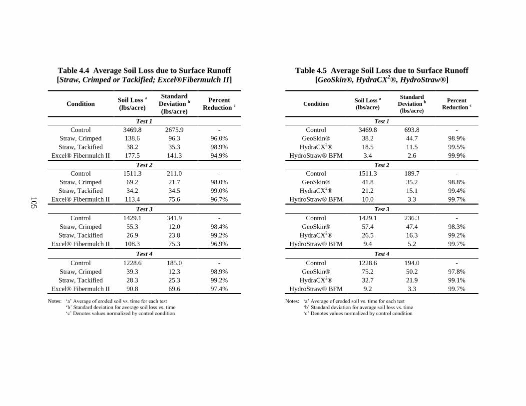
105
Table 4.4 Average Soil Loss due to Surface Runoff
[Straw, Crimped or Tackified; Excel®Fibermulch II]
Condition Soil Loss
a
(lbs/acre)
Standard
Deviation b
(lbs/acre)
Percent
Reduction c
Test 1
Control 3469.8 2675.9 -
Straw, Crimped 138.6 96.3 96.0%
Straw, Tackified 38.2 35.3 98.9%
Excel® Fibermulch II 177.5 141.3 94.9%
Test 2
Control 1511.3 211.0 -
Straw, Crimped 69.2 21.7 98.0%
Straw, Tackified 34.2 34.5 99.0%
Excel® Fibermulch II 113.4 75.6 96.7%
Test 3
Control 1429.1 341.9 -
Straw, Crimped 55.3 12.0 98.4%
Straw, Tackified 26.9 23.8 99.2%
Excel® Fibermulch II 108.3 75.3 96.9%
Test 4
Control 1228.6 185.0 -
Straw, Crimped 39.3 12.3 98.9%
Straw, Tackified 28.3 25.3 99.2%
Excel® Fibermulch II 90.8 69.6 97.4%
Notes: ‗a‘ Average of eroded soil vs. time for each test
‗b‘ Standard deviation for average soil loss vs. time ‗c‘ Denotes values normalized by control condition
Table 4.5 Average Soil Loss due to Surface Runoff
[GeoSkin®, HydraCX2®, HydroStraw®]
Condition Soil Loss a
(lbs/acre)
Standard
Deviation b
(lbs/acre)
Percent
Reduction c
Test 1
Control 3469.8 693.8 -
GeoSkin® 38.2 44.7 98.9%
HydraCX2® 18.5 11.5 99.5%
HydroStraw® BFM 3.4 2.6 99.9%
Test 2
Control 1511.3 189.7 -
GeoSkin® 41.8 35.2 98.8%
HydraCX2® 21.2 15.1 99.4%
HydroStraw® BFM 10.0 3.3 99.7%
Test 3
Control 1429.1 236.3 -
GeoSkin® 57.4 47.4 98.3%
HydraCX2® 26.5 16.3 99.2%
HydroStraw® BFM 9.4 5.2 99.7%
Test 4
Control 1228.6 194.0 -
GeoSkin® 75.2 50.2 97.8%
HydraCX2® 32.7 21.9 99.1%
HydroStraw® BFM 9.2 3.3 99.7%
Notes: ‗a‘ Average of eroded soil vs. time for each test
‗b‘ Standard deviation for average soil loss vs. time ‗c‘ Denotes values normalized by control condition

106
Continuing the statistical analysis used throughout this research effort, ANOVA
procedures with Tukey-Kramer multiple comparison tests were used for the recorded
amounts of soil. Table 4.6 illustrates statistically significant and insignificant results of
average soil loss throughout the experiments. The statistical analysis compared all
treatments to the control and each other. The control proved to be statistically different
than all treatments; therefore each treatment had a significant effect in reducing soil loss
when compared the bare soil. When the treatments were compared amongst each other
all were capable of reducing soil loss significantly the same. Therefore it can be
concluded from Table 4.6 that statistically, each treatment is capable of significantly
reducing and controlling erosion on 3H:1V, compacted fill slopes.

107
Table 4.6 Tukey-Kramer Comparison on Average Soil Loss
Comparison µi - µj CI [LB] CI [UB] Significantly
Different C
on
tro
l GeoSkin 1,857 1,312 2,401 Yes
Straw, Crimped 1,834 1,289 2,379 Yes
HydraCX2 1,885 1,340 2,430 Yes
Excel Fibermulch II 1,787 1,242 2,332 Yes
HydroStraw BFM 1,902 1,357 2,447 Yes
Straw, Tackified 1,878 1,333 2,423 Yes
Str
aw
,
Cri
mp
ed
Control 1,834 1,289 2,379 Yes
GeoSkin 22 -522 567 No
HydraCX2 51 -494 596 No
Excel Fibermulch II 47 -498 592 No
HydroStraw BFM 68 -477 612 No
Straw, Tackified 44 -501 589 No
Str
aw
,
Ta
ckif
ied
Control 1,878 1,333 2,423 Yes
GeoSkin 21 -524 566 No
Straw, Crimped 44 -501 589 No
HydraCX2 7 -538 552 No
Excel Fibermulch II 91 -454 635 No
HydroStraw BFM 24 -521 569 No
Geo
Sk
in
Control 1,857 1,312 2,401 Yes
Straw, Crimped 22 -522 567 No
HydraCX2 28 -516 573 No
Excel Fibermulch II 69 -476 614 No
HydroStraw BFM 45 -500 590 No
Straw, Tackified 21 -524 566 No
Hy
dra
CX
2
Control 1,885 1,340 2,430 Yes
Straw, Crimped 51 -494 596 No
GeoSkin 28 -516 573 No
Excel Fibermulch II 98 -447 643 No
HydroStraw BFM 17 -528 562 No
Straw, Tackified 7 -538 552 No
Ex
cel
Fib
erm
ulc
h I
I Control 1,787 1,242 2,332 Yes
Straw, Crimped 47 -498 592 No
GeoSkin 69 -476 614 No
HydraCX2 98 -447 643 No
HydroStraw BFM 114 -430 659 No
Straw, Tackified 91 -454 635 No
Hy
dro
Str
aw
BF
M
Control 1,902 1,357 2,447 Yes
Straw, Crimped 68 -477 612 No
HydraCX2 17 -528 562 No
Excel Fibermulch II 114 -430 659 No
GeoSkin 45 -500 590 No
Straw, Tackified 24 -521 569 No
Notes: [LB] signifies lower bound of confidence interval = -545
[UB] signifies upper bound of confidence interval = +545
qcrit = 4.18

108
4.2.4 Initial Turbidity vs. Soil Loss
To determine the relationship between the average recorded initial turbidities (essentially
indicative of reducing sediment transport or migration) and average measured soil loss
(which is indicative of erosion control performance) values were plotted together,
illustrated in Figure 4.8. Average soil loss and initial turbidity values for the control
produced an outlying group of high sediment yield and turbidity values, shown on the far
right side of the plot, making it difficult to distinguish the performance of the other
treatments tested. Therefore Figure 4.9 was created without the control to present the
other treatments in a more comparable manner.
Figure 4.8 Average Initial Turbidity vs. Average Eroded Soil.
0
1000
2000
3000
4000
5000
6000
7000
8000
0 1000 2000 3000 4000 5000 6000 7000 8000
Ero
ded
So
il (lb
s/a
cre)
Turbidity (NTU)
Control GeoSkin Straw, Crimped HydraCX2 Excel Fibermulch II HydroStraw BFM Straw, Tackified

109
As illustrated in Figure 4.9, the three treatments that were not statistically different are
ranked in order of percent reduction (i.e., soil loss and initial turbidity) in comparison to
the control: (1) HydroStraw® BFM, (2) conventional straw with a tackifier, and (3)
HydraCX2®. The relationship between initial turbidities can be used as a method to
determining overall performance of a treatment from an erosion and/or sediment
transport perspective. Patterns and consistencies in erosion and sediment transport
control are also revealed when using this method to plot treatments. For example,
Excel® Fibermulch II and ‗Straw, Crimped‘ have plotted values with a wider variability
in comparison to the other treatments, showing signs of inconsistencies in product
performance. Overall, significant reductions in both soil loss and initial turbidity are
observed for each treatment when compared to the bare soil condition, as illustrated in
Figure 4.8 and Figure 4.9.

110
Figure 4.9 Average Initial Turbidity vs. Average Eroded Soil [Excludes Control].
4.2.5 Cover-Factor
Studies reviewed (Lipscomb et al., 2006; Holt et al., 2005; Landloch, 2002; Clopper et
al., 2001; Buxton and Caruccio, 1979) used a ‗cover-factor‘ to report erosion control
performance. Cover factor is a parameter in the Revised Universal Soil Loss Equation
(RUSLE) to represent a comparison of soil loss occurring with the treatment in place to
that which occurs in the bare, unprotect condition (Clopper et al., 2001). The RUSLE
allows researchers to calculate cover-factors for treatments without testing a bare soil
using several different parameters based upon soil type, slope, and rain regimes;
Lipscomb et al. (2006) and Clopper et al. (2001) mitigated the RUSLE to calculate cover-
factors. However, if bare soil conditions are accounted for, the cover-factor is simply the
0
50
100
150
200
250
300
0 500 1000 1500 2000 2500 3000
So
il L
oss
(lb
s/a
cre)
Turbidity (NTU)
GeoSkin Straw, Crimped HydraCX2 Excel Fibermulch II HydroStraw BFM Straw, Tackified

111
ratio of sediment yield in the protected condition to sediment yield of the unprotected
condition; Holt et al. (2005) effectively used this method to calculate c-factors. In 1979,
Buxton and Caruccio used the Universal Soil Loss Equation (USLE) to calculate cover-
factor values, which were at the time identified as ‗VM factors‘. In 1979, a VM factor
represented a vegetative or maintenance erosion control practice and was a total soil loss
ratio expressed as a decimal. Landloch (2002) calculated cover-factors using the
Modified Universal Soil Loss Equation (MUSLE), which calculates erosive potential as a
factor W, which is based on rainfall erosivity, peak runoff rate, total runoff, slope
gradient and length, cover, etc.
Although there are several methods to calculating cover-factors, cover-factor remains
simply a soil loss ratio (SLR) of treated to untreated (bare soil) conditions. Cover-factors
numerically represent erosion control performance on a scale of 0.0 to 1.0, where a value
of 0.0 means the erosion control practice has eliminated all erosion, and a cover-factor of
1.0 means the practice has done nothing to reduce erosion and is equivalent to a bare soil
condition. Table 4.7 summarizes the cover-factors calculated in this research effort,
normalized to bare soil conditions. According to calculated cover-factors of 0.004,
0.013, 0.017, 0.028 0.040, and 0.064 in Table 4.7, the hydromulches can be ranked from
most to least effective erosion control practices accordingly: (1) HydroStraw® BFM, (2)
HydraCX2®, (3) Conventional Straw, Tackified, (4) GeoSkin®, (5) Conventional Straw,
Crimped, and (6) Excel® Fibermulch II; however there are no statistical differences
between practices.

112
Table 4.7 Cumulative Soil Loss (A) to Calculate Cover Factors (C) per Treatment
Treatment Cumulative Soil Loss
(A) (grams/plot)1
Cumulative Soil Loss
(A) (tons/acre)2
*Calculated Cover
Factor (C)3
HydroStraw® BFM 13 36 0.004
HydraCX2® 41 112 0.013
Conventional Straw,
Tackified 53 145 0.017
GeoSkin® 89 241 0.028
Conventional Straw,
Crimped 126 343 0.040
Excel® Fibermulch II 204 556 0.064
Note: ‗1‘ Unit conversion: 1 gram/plot = 0.035 oz/plot.
‗2‘ Unit conversion: 1 ton/acre = 2242 kg/ha. ‗3‘ Cover factor normalized to a bare soil value of 8,662 tons/acre (19,420,204 kg/ha).
‗*‘ Cover factor calculation: C=A/Control3.
4.3 Summary
Data collection from intermediate-scale experiments allowed researchers to observe and
evaluate the performance of conventional straw (crimped or tackified) and four
hydromulches (Excel® Fibermulch II, GeoSkin®, HydraCX2®, and HydroStraw® BFM)
as an erosion control measure. Data collection included: (1) surface runoff, (2) initial
turbidity, (3) turbidity versus time, and (4) soil loss. The collected data was analyzed
using ANOVA and Tukey-Kramer statistical analysis procedures to determine the effect
of different treatments and if any statistical significant results were observed.
At total of 1,680 runoff samples were recorded for 14 experiments in this research effort.
This consisted of samples collected every minute for all four rainfall events per
experiment. Initial turbidity measurements were recorded from every sample collected,
allowing researchers to rank treatments; from most to least effective in reducing turbidity

113
when normalized to bare soil (control) conditions, the ranked treatments in this research
effort are (1) HydroStraw® BFM, (2) straw, tackified, (3) HydraCX2®, (4) GeoSkin®,
(5) Excel® Fibermulch II, and (6) straw, crimped, with reductions of 99%, 98%, 95%,
92%, 85%, and 80% respectively. The straw treatments without tackifiers, conventional
straw, crimped and Excel® Fibermulch II, experienced the ‗first-flush‘ phenomenon,
receiving an initial surge of concentrated sediment in the runoff, which steadily reduced
over time. Contrarily, the hydromulches and straw with tackifier were observed to
slowly lose their effectiveness over the four rainfall events as the chemical bonds in the
tackifying agents began to deteriorate.
In addition, soil loss samples were collected every 3 minutes from surface runoff, totaling
560 samples, to determine an amount of eroded soil from test plots. Samples were
filtered and oven dried for 24 hours. Soil loss reduction results included 100%, 99%,
98%, 97%, 96%, and 94% for HydroStraw® BFM, HydraCX2®, straw-tackified,
GeoSkin®, straw-crimped, and Excel® Fibermulch II respectively. Figure 4.10 is a bar
chart representing the average percent reduction of turbidity and soil loss for each
treatment normalized to the bare soil control in this research effort.
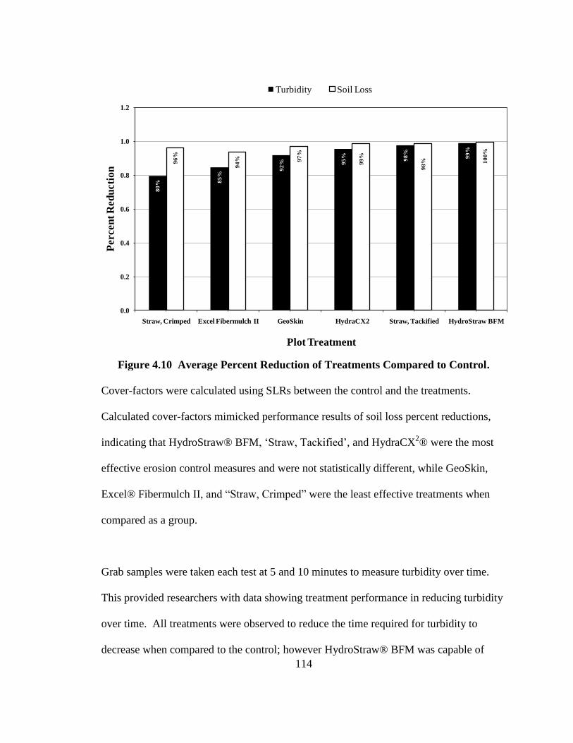
114
Figure 4.10 Average Percent Reduction of Treatments Compared to Control.
Cover-factors were calculated using SLRs between the control and the treatments.
Calculated cover-factors mimicked performance results of soil loss percent reductions,
indicating that HydroStraw® BFM, ‗Straw, Tackified‘, and HydraCX2® were the most
effective erosion control measures and were not statistically different, while GeoSkin,
Excel® Fibermulch II, and ―Straw, Crimped‖ were the least effective treatments when
compared as a group.
Grab samples were taken each test at 5 and 10 minutes to measure turbidity over time.
This provided researchers with data showing treatment performance in reducing turbidity
over time. All treatments were observed to reduce the time required for turbidity to
decrease when compared to the control; however HydroStraw® BFM was capable of
80
% 85
%
92
% 95
%
98
%
99
%
96
%
94
% 97
%
99
%
98
% 10
0%
0.0
0.2
0.4
0.6
0.8
1.0
1.2
Straw, Crimped Excel Fibermulch II GeoSkin HydraCX2 Straw, Tackified HydroStraw BFM
Percen
t R
ed
ucti
on
Plot Treatment
Turbidity Soil Loss

115
meeting ADEM ELGs of 50 NTUs, and straw, tackified and HydraCX2® were capable of
meeting the USEPA ELG of 280 NTUs.
Overall, according to experimental results, it was observed that there were no statistical
differences in performance from an erosion control perspective between HydroStraw®
BFM, ‗Straw, Tackified‘, and HydraCX2®, which all have potential to be effective
erosion control practices. This was observed using recorded and analyzed turbidity
measurements and soil loss masses collected from test plot runoff.
116
Chapter 5 Conclusions and Recommendations
5.
5.1 Introduction
The purpose of this research effort was to evaluate the erosion control performance of the
following four hydromulches: (1) Excel® Fibermulch II, (2) GeoSkin®, (3)
HydraCX2®, and (4) HydroStraw® BFM, in comparison to a bare soil control and two
conventional straw practices that were either crimped or tackified. To achieve this,
intermediate-scale experimentations were conducted to simulate conditions representative
of a typical highway embankment with a fill slope of 3H:1V. The first objective involved
the design and construction of a flume to modify Shoemaker‘s (2009) runoff collection
device on the intermediate-scale (2 ft by 4 ft [0.6 m by 1.2 m]) plots. Once the flume was
constructed, research and development of a uniform and consistent method of applying
the 4 hydromulch and 2 conventional straw treatments was completed to ensure accurate,
quantifiable, manufacture specified application rates. The second component of this
research used the unified test procedures developed to evaluate the effectiveness of the 6
treatments. The data collected from the compacted, 3H:1V test plots was compared to a
bare soil (control) condition and analyzed to provide recommendations for use of
conventional straw (crimped or tackified) and hydromulches on highway construction
sites.

117
5.2 Intermediate-Scale Test Methods and Procedures
Intermediate-scale experimental procedures and methods of data collection were adopted
from Shoemaker (2009). A flume was designed and constructed to modify the collection
runoff device used on the 2 ft (0.6 m) wide by 4 ft (1.2 m) long test plots. Uniform
runoff was created by a rainfall simulator, verified by Shoemaker (2009) using the
Christiansen Uniformity Coefficient to have an acceptable uniformity ranging between
84% and 88%. Experiments were divided into four 15 minute tests with 15 minute
breaks in between for optimal data collection. The four tests produced a total rainfall of
approximately 4.4 inches (1.1 inches per test) of rain, meeting the ALDOT‘s inspection
guidelines that state ESC practices must be inspected following an accumulated amount
of rainfall measuring 0.75 in. The rainfall event produced in this research effort was
indicative of a 2-year, 24 hour storm event experienced in Auburn, AL with a total
rainfall amount of 4.39 in/hr.
Another essential task to properly test the effectiveness of ESC practices in this research
effort involved compacting the test soil to ALDOT‘s standard specified rate of 95%. It
was determined by a soil and compaction analysis that hand-tamps were capable of
compacting the test soil at an OMC of 14% to achieve the required rate of 105 pcf (1,682
kg/m3) for compaction. Once the intermediate-scale test plots were compacted and
scoured to simulate typical highway embankments, the plots were ready for ESC
treatments to be applied.
A uniform and consistent method of applying each treatment was researched and
evaluated individually to ensure proper, manufacture specified application rates.

118
Application procedures for applying conventional straw crimped or tackified to 3H:1V
slopes was followed using methods developed by ALDOT (2008). However, applying
the hydromulches was more involved therefore a procedure was developed to determine
the application rate per spray (using a hydroseeder), allowing researchers to verify the
application rate after a predetermined amount of sprays. Methods developed were used
to ensure manufacturer specified application rates were achieved.
Once the treatments were uniformly applied and allowed a 48 hour drying period under
ultra-violet ray heat lamps, testing could begin. A turbidity meter was used to record
initial turbidity measurements as well as turbidity over time for all experiments,
representative of controlling sediment migration in construction stormwater runoff from
typical highway embankments. Runoff samples were filtered, dried for 24 hours, and
weighed to account for sediment loss (erosion control). With the recorded data,
researchers could properly evaluate the performance of each treatment.
5.3 Performance of Conventional Straw and Hydromulch
Fourteen experiments were conducted to examine the erosion control effectiveness of 4
hydromulch practices and 2 conventional straw surface cover practices: (1) Excel®
Fibermulch II, (2) GeoSkin®, (3) HydraCX2®, (4) HydroStraw® BFM, (5) conventional
straw, crimped, (6) conventional straw, tackified. Performance was evaluated using data
collection from experiments, which included surface runoff volume and mass, initial
turbidity, and turbidity over time.

119
Initial turbidity measurements were recorded from samples that were collected every
minute of each four, 15 minute rainfall events. Representative of initial sediment control,
researchers were able to rank the 6 treatments in order from most to least effective
according to an averaged percent reduction when normalized by the bare soil condition:
(1) HydroStraw® BFM [99% reduction], (2) straw, tackified [98% reduction], (3)
HydraCX2® [95% reduction], (4) GeoSkin® [92% reduction], (5) Excel® Fibermulch II
[85% reduction], and (6) straw, crimped [80% reduction]. The surface cover practices
without tackifiers, conventional straw, crimped and Excel® Fibermulch II, experienced a
heavy concentration of sediment in the runoff during the first two rainfall events, which
is known as the ‗first flush phenomenon‘; however each treatment steadily improved
sediment transport control over time. Contrarily, the surface cover practices with
tackifying agents provided excellent initial sediment transport control, but over the four
rainfall events the chemical bonds began to deteriorate, showing a steady decrease in
performance.
Grab samples were collected from each test at 5 and 10 minutes to measure turbidity over
time. Each treatment was observed to reduce the time required for turbidity to decrease
when compared to the control. It was observed that the most effective treatment reducing
turbidity over the 200 second settling period was the HydroStraw® BFM, which was also
the only product to meet the ADEM effluent limitation guidelines (ELGs) of 50 NTUs.
‗Straw, Tackified‘ and HydraCX2 were able to meet the USEPA new ELGs of 280 NTUs,
recording 5 and 10 minute final values of 61.8 and 60.2 NTUs, and 17.5 and 14.4 NTUs,
respectively for each treatment.
120
Once initial turbidity measurements and turbidity over time grab samples were taken,
collective runoff over a 3 minute period was filtered, oven dried for 24 hours, and
weighed to provide quantitative erosion control results. Researchers observed
approximately 100%, 99%, 98%, 97%, 96%, and 94% for HydroStraw® BFM,
HydraCX2®, straw-tackified, GeoSkin®, straw-crimped, and Excel® Fibermulch II
respectively. Cumulative soil losses were also used in this research to calculate cover-
factors, which are SLRs between treated and untreated conditions; calculated c-factors
mimicked percent reduction performances, ranging in value from 0.004 for HydroStraw®
BFM to 0.064 for Excel® Fibermulch II.
Literature reviewed and results from this research suggest that conventional straw
crimped or tackified as well as hydromulches are very effective erosion control measures,
when applied at the proper application rates. According to experimental results,
HydroStraw® BFM was the only hydromulch practice that was able to satisfy both
USEPA (280 NTUs) and ADEM (50 NTUs above background turbidity levels) ELGs.
For all other treatments, sediment control additives such as polyacrylamide (PAM) are
encouraged to be used in conjunction for optimal erosion and sediment transport control
on construction sites with 3H:1V compacted fill slopes.
It is to be recognized that there are five qualifying experimental factors that have an
impact on the conclusions drawn from the results reported from this research, which
include: (1) soil type, (2) slope, (3) soil compaction, (4) rainfall simulator, and (5)

121
rainfall intensity. These qualifying factors were designed into the experimental
procedures and have the potential to create a biased outcome on some conclusions and
recommendations that can be made for the erosion control practices tested. It should also
be noted the intermediate-scale results reported herein may not be scale-able to field-
scale or practical-scale performance on active construction sites.
5.4 Recommended Future Research
Results presented in this report show that conventional straw crimped or tackified and
hydromulches are effective means of reducing erosion and sedimentation caused by
sediment laden runoff. However, conventional straw or hydromulches are rarely used on
its own and is more commonly used in conjunction with additional sediment control
additives such as PAM. Therefore, further research should be conducted to examine how
the addition of PAM to these practices could potentially improve ESC performance.
Also, the conclusions discussed in this report are based on intermediate-scale test plots.
It would be beneficial if the performance of these treatments were tested at field-scale
conditions to validate intermediate-scale results provided in this research. Intermediate-
scale experiments allow researchers to test the performance of ESC practices at a faster
rate than most field-scale experiments; therefore, if field-scale results were found to be
similar to intermediate-scale results, a larger quantity of products could be effectively
evaluated in a shorter period of time.

122
Lastly, this research only tested the performance of 4 manufactured hydromulch
products. Increased technologies over the years have allowed for the creation of many
new hydromulches that claim to be the best product on the market. It is strongly
encouraged to further investigate the performance of other hydromulch products on the
market to create a more thorough analysis and to provide a more scientific realm of
knowledge of the hydromulch industry.

123
References
1. Aicardo, R. (1996). Screening of Polymers to Determine Their Potential Use in
Erosion Control on Construction Sites. In Proceedings from Conference held at
College of Southern Idaho: Managing Irrigation-Induced Erosion and Infiltration
with Polyacrylamide, May 6-8, 1996, Twin Falls, ID. University of Idaho
Miscellaneous Publication No. 101-96.
2. Alabama Department of Environmental Management (ADEM). Alabama
Environmental Regulations and Laws. <
http://www.adem.state.al.us/alEnviroRegLaws/default.cnt>. Montgomery: AL,
2010a.
3. Alabama State. Alabama Soil and Water Conservation Committee (ASWCC).
Alabama Handbook for Erosion Control, Sediment Control, and Stormwater
Management on Construction Site and Urban Areas: Volume 2. Montgomery:
Alabama, 2009.
4. American Society for the Testing of Materials (ASTM), (2000). ASTM D-6459:
Standard Test Method for Determination of Erosion Control Blanket (ECB)
Performance in Protecting Hillslopes from Rainfall-Induced Erosion. ASTM, West
Conshohocken, PA. January.
5. Babcock, D. and McLaughlin (2008). Mulch Options for Erosion Control on
Construction Sites. Date Accessed: 8 October, 2010.
<http://www.soil.ncsu.edu/publications/Soilfacts/AG-439-67W/>.
6. Barnett, A. P., Diseker, E. G., and Richardson, E. C. (1967). Evaluation of mulching
methods for erosion control on newly prepared and seeded highway backslopes,
Agronomy Journal, 59, 83-85.
7. Benik, S. R., B.N. Wilson, et al. (2003) Performance of erosion control products on a
highway embankment. Transactions of the ASAE, 46(4): 1113–1119.
8. Bjorneberg, D. L., J. K. Aase, et al. (2000). Controlling sprinkler irrigation runoff,
erosion, and phosphorus loss with straw and polyacrylamide. Transactions of the ASAE,
43(6): 1545-1551.Box, J. E., Jr. and Bruce, R. R (1996). The effect of surface cover on
infiltration and soil erosion, pp. 107-123 in M. Aggasi (ed.), Soil Erosion,
Conservation and Rehabilitation, Dekker, New York.

124
9. Brady, N.C. and R.R. Weil (1996). The Nature and Properties of Soils, 11th
edition.
Upper Saddle River, NJ: Prentice Hall.
10. Bruce, R.R., G.W. Langdale, L.T. West, and W.P. Miller (1995). Surface Soil
Degradation and Soil Productivity Restoration and Maintenance. Soil Science
Society of America Journal 59: 654-660.
11. Burroughs, E.R. and King, J.G. (1989). Reduction of Soil Erosion on Forest Roads.
United States Department of Agriculture, Forest Service Intermountain Research
Station. General Technical Report INT-264.
12. Buxton, H. and Caruccio, F. T. (1979). Evaluation of Selective Erosion Control
Techniques. Piedmont Region of S.E. United States, US Environmental Protection
Agency EPA-600/2-79-124, Cincinnati, OH.
13. Clopper, P.E., Vielleux, M., Johnson,T. (2001). Quantifying the Performance of
Hillslope Erosion Control Best Management Practices:, ASCE.
14. Dudeck, A. E., Swanson, N. P., Mielke, L. N. and Dedrick, A. R. (1970). Mulches
for grass establishment on fill slopes, Agronomy Journal, 62, 810-812.
15. Erosion Control Technology Council (ECTC) (2008). Erosion control product
categories. <http://www.ectc.org/erosion_control_categories.asp#hecp>.
16. Faucette, B (2004).Evaluation of Environmental Benefits and Impacts of Compost
and Industry Standard Erosion and Sediment Controls Measures Used in
Construction Activities. Dissertation, Institute of Ecology, University of Georgia,
Athens, Georgia.
17. Faucette, B. and M. Risse. (2002). Controlling Erosion with Compost and Mulch.
BioCycle, June 2002, pages 26–28.
18. Harding, M. V. (1988). Erosion control effectiveness: Comparative studies of
alternative mulching techniques, Transportation Research Board, 67th Annual
Meeting, 11-19 January, Paper No. 870244, Washington, DC.
19. Holt, G.A. and J.W. Laird (2002). COBY products and a process for their
manufacture. U.S. Patent No. 6,383,548. Date issued: 7 May 2002.
20. Holt, G.A., Buser, M., Harmel, D., Potter, K., and Pelletier, M. (2005) Comparison
of Cotton-based Hydro-mulches and Conventional Wood and Paper Hydro-mulches-
Study 1. The Journal of Cotton Science, 9:121-127.

125
21. Horner, R. R., Guedry, J. and Kortenhof, M. H. (1990). Improving the Cost
Effectiveness of Highway Construction Site Erosion and Pollution Control. Final
Report, Research Project GC 8286, Task 7, Construction Erosion Control-II,
Washington State Transportation Center, Report No. WA-RD 200.1, Olympia, WA.
22. Kayhanian, M. and Stenstrom, M.K. (2008). First-Flush Characterization for
Stormwater Treatment. <http://www.stormh2o.com/march-april-2008/pollutants-run-
off.aspx>.
23. Lancaster, T. and Theisen, M (2004). Classifying rolled erosion control products: a
current perspective. The Erosion Control Technology Council (ECTC). St. Paul:
MN. Date Accessed: 8 October 2010.
<http://www.ectc.org/resources/ClassRECP04.pdf>.
24. Landloch (2002). Studies of Hydromulch Effectiveness. National Centre for
Engineering in Agriculture Publication 1000455/1, USQ, Toowoomba.
25. Lipscomb, C.M., Johnson, T., Nelson, R, and Lancaster, T. (2006). Comparison of
Erosion Control Technologies: Blown Straw vs. Erosion Control Blankets. Land
And Water.
26. Mannering, J.V. and L.D. Meyer (1963). The Effects of Various Rates of Surface
Mulch on Infiltration and Erosion. Soil Science Society of America Journal 29: 84-
85.
27. Mayo, L., D. Lehman, L. Olinger, B. Donavan, and P. Mangarella. (1993). Urban
BMP Cost and Effectiveness Summary Data for 6217(g) Guidance: Erosion and
Sediment Control During Construction. Woodward-Clyde Consultants.
28. McLaughlin, R. A. and T. T. Brown (2006). Evaluation of erosion control products
with and without added polyacrylamide. Journal of the American Water Resources
Association, 42(3): 675-684.
29. Meyer, L.D., W.H. Wischmeier, and G.R. Foster (1970). Mulch Rates Required for
Erosion Control on Steep Slopes. Soil Science Society of America, Proceedings
34:928-930.
30. Morgan, R. and Rickson, J. (1988). Soil erosion control: Importance of
geomorphological information, pp. 51-60 in J. M. Hooke (ed.) Geomorphology in
Environmental Planning, Wiley, Chichester.
31. National Cooperative Highway Research Program (NCHRP) (1980). Erosion Control
During Highway Construction—Research Report, Transportation Research Board,
National Research Council, Report No. 220, Washington, DC.

126
32. Novotny, Vladimir. Water Quality: Diffuse Pollution and Watershed Management.
New York: John Wiley & Sons, Inc., 2003.
33. Parsons, T.S., Burney, J.R., and Edwards, L. (1994). Field measurement of soil-
erodibility and cover-management factors in Prince Edward Island using simulated
rainfall. Canadian Agricultural Engineering, Vol. 36, No. 3, pp 127-133.
34. Rickson, R. J. (1995). Simulated vegetation and geotextiles, pp. 95-131 in R. P. C.
Morgan and R. J. Rickson (eds.) Slope Stabilization and Erosion Control: A
Bioengineering Approach, Spon, London.
35. Risse, M. and B. Faucette. 2001. Compost Utilization for Erosion Control.
University of Georgia Cooperative Extension Service Bulletin 1200. Athens, GA:
Cooperative Extension Service, University of Georgia.
36. Shoemaker, A. L. (2009). Evaluation of Anionic Polyacrylamide as an Erosion
Control Measure Using Intermediate-Scale Experimental Procedures. MS Thesis,
Auburn University.
37. Singer, M.T., Y. Matsuda, and J. Blackard (1981). Effect of Mulch Rate on Soil Loss
by Raindrop Splash. Soil Science Society of America Journal 45:107-110.
38. Sutherland, R.A. and Ziegler, A.D. (2006). Hillslope runoff and erosion as affected
by rolled erosion control systems: a field study. Hydrological Processes: 20, 2839–
2855.
39. Sutherland, RA (1998). Rolled erosion control systems for hillslope surface
protection: a critical review, synthesis and analysis of available data. I. Background
and formative years. Land Degradation and Development 9: 465–486.
40. Turgeon, A.J. (2002). Turfgrass Management, Sixth Edition. Prentice Hall, Upper
Saddle River, New Jersey.
41. United States Environmental Protection Agency (U.S. EPA). Stormwater
Management for Industrial Activities: Developing Pollution Prevention Plans and
Best Management Practices. U.S. Environmental Protection Agency, Washington:
D.C., 1992.
42. United States Environmental Protection Agency (U.S. EPA). Guidance Specifying
Management Measures for Sources of Nonpoint Pollution in Coastal Waters. EPA
840-B-92-002. U.S. Environmental Protection Agency, Office of Water, Washington,
D.C. 1993.
127
43. United States Environmental Protection Agency (U.S. EPA). Innovative Uses of
Compost: Erosion Control, Turf Remediation and Landscaping. EPA 530-F-97-043.
Washington, DC., 1997.
44. United States Environmental Protection Agency (U.S. EPA). 2000 National Water
Quality Inventory. EPA 841/R-02/001. Office of Water, Washington: D.C., 2000.
45. United States Environmental Protection Agency (U.S. EPA). Stormwater Phase II
Final Rule: An Overview. EPA 833/F-00/001. Office of Water, Washington: D.C.,
2005a.
46. United States Environmental Protection Agency (U.S. EPA). Stormwater Phase II
Final Rule: Construction Site Runoff Control Minimum Control Measure. EPA
833/F-00/008. Office of Water, Washington: D.C., 2005b.
47. United States Environmental Protection Agency (U.S. EPA). Effluent Limitations
Guidelines and Standards for the Construction and Development Point Source
Category. EPA Federal Register, 73(230): 72561-72614. Washington: D.C., 2008.
48. United States Environmental Protection Agency (U.S. EPA). Economic Analysis for
Final Effluent Guidelines and Standards for the Construction and Development
Category. (EPA-821-R-09-011). Office of Water, Washington: D.C., 2009a.
49. United States Environmental Protection Agency (U.S. EPA). Environmental Impact
and Benefits Assessment for Final Effluent Guidelines and Standards for the
Construction and Development Category. (EPA-821-R-09-012). Office of Water,
Washington: D.C., 2009b.
50. United States Environmental Protection Agency (U.S. EPA). Final Rule: Effluent
Guidelines for Discharges from the Construction and Development Industry. EPA
821/F-09/004. Office of Water, Washington: D.C., 2009c.
51. United States Environmental Protection Agency (U.S. EPA). A Brief Summary of the
History of NPDES. Office of Water, Washington: D.C.. Date Accessed: 10 October
2010a. <http://www.epa.gov/region1/npdes/history.html>.
52. United States Environmental Protection Agency (U.S. EPA). National Pollutant
Discharge Elimination System (NPDES): Construction Site Stormwater Runoff
Control. . Washington: D.C., 2006. Date Accessed: 10 October 2010b.
<http://www.epa.gov/npdes/stormwater/menuofbmps/construction>
53. Weggel, J. R. and Rustom, R. (1992). Soil erosion by rainfall and runoff—State of
the art, Geotextiles and Geomembranes, 11, 551-572.

128
54. Zech, W.C., Halverson, J.L., and Clement, T.P. “Evaluating the Effectiveness of
Various Types of Silt Fence Installations to Control Sediment Discharge from
Highway Construction Sites”, ASCE Journal of Hydrologic Engineering, June 2008,
Vol. 13, No. 6, pp 497-504.
55. Zech, W.C., Halverson, J.L., and Clement, T.P. “Development of a Silt Fence
Tieback Design Methodology for Highway Construction Installations”,
Transportation Research Record, No. 2011, Journal of the Transportation Research
Board, 2007, pp 21-28.

129
Appendix 1 Manufacturer’s Specifications for Rainfall Simulator Components

130
Pressure Regulator

131
Solenoid Valve (a)

132
Solenoid Valve (b)
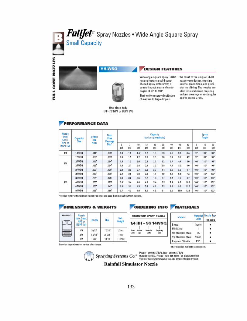
133
Rainfall Simulator Nozzle

134
Raindrop Sizes

135
Appendix 2 Rainfall Intensity-Duration-Frequency Curves for Alabama.
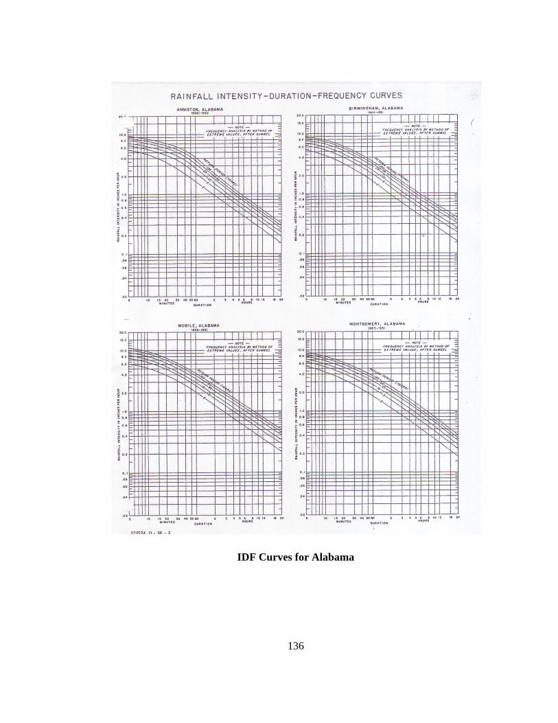
136
IDF Curves for Alabama

137
(a) 2-yr, 24-hr Cumulative rainfall for the United States
(b) 2-yr, 24-hr Cumulative rainfall for Alabama

138
Appendix 3 Manufacturer’s Specifications for Equipment Used During
Experimentation

139
Backpack Sprayer

140
Turbidity Meter (a)
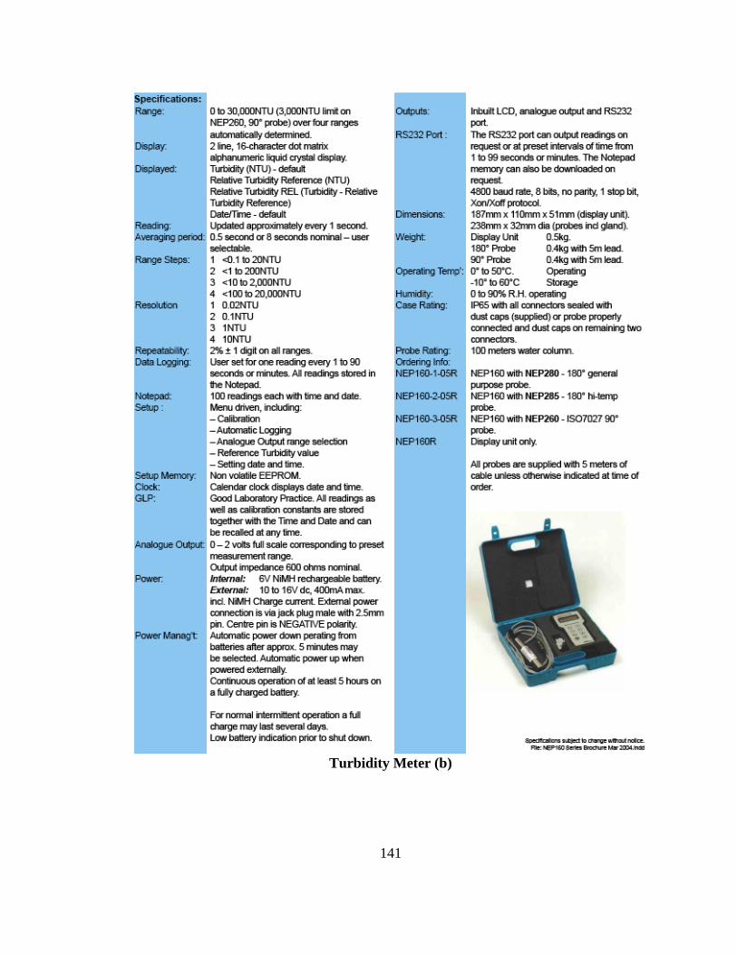
141
Turbidity Meter (b)

142
Appendix 4 Hydromulch Manufacturer Specifications

143
HydroStraw® BFM Specifications
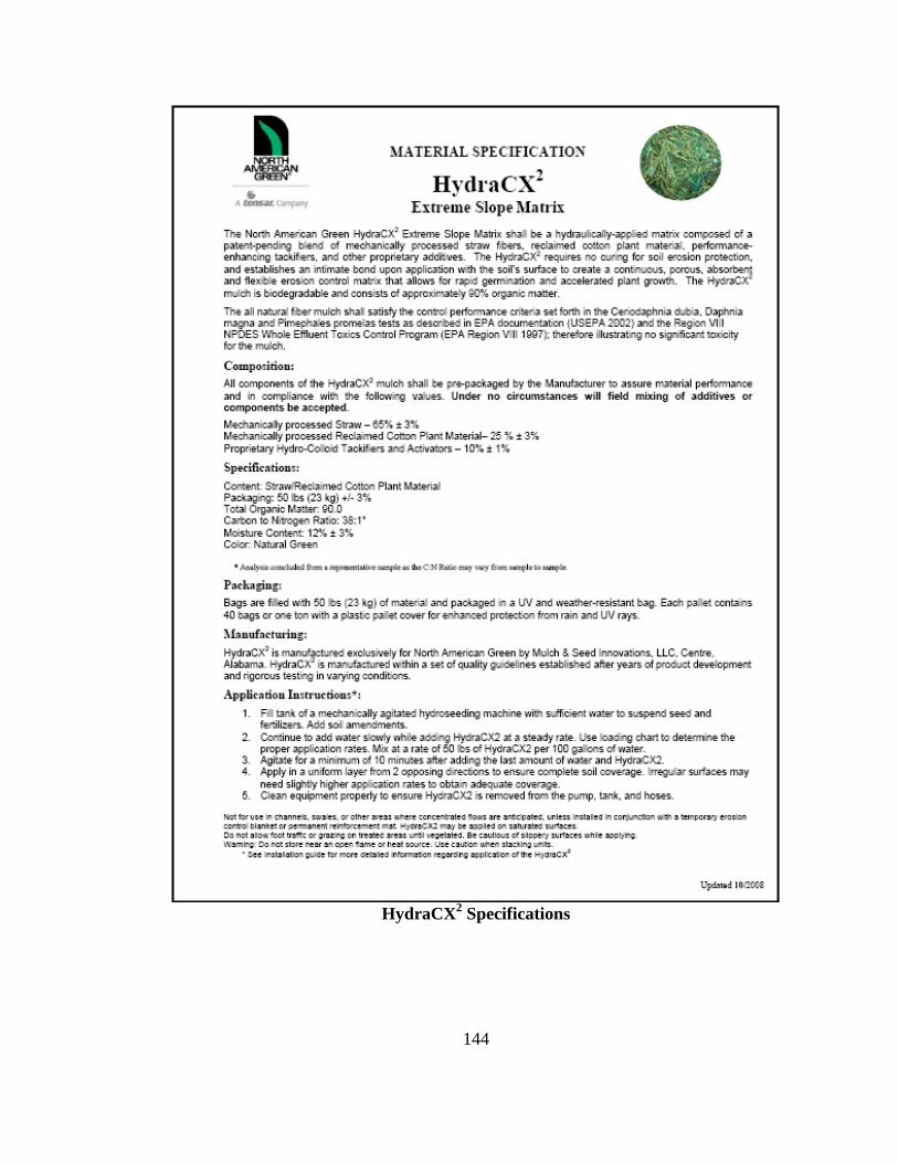
144
HydraCX
2 Specifications

145
GeoSkin® Specifications

146
Excel® Fibermulch II Specifications

147
Hytac II Acrylic Tackifier

148
Appendix 5 Hydromulch Experimentation

149
EXCEL® FIBERMULCH II
Post-Application of Excel® Fibermulch II (a)
Post-Application of Excel® Fibermulch II (b)

150
EXCEL® FIBERMULCH II
Post-48 hour Drying Period
Post-Experimentation (2yr, 24 hr storm)

151
GEOSKIN®
Post-Application of GeoSkin® (a)
Post-Application of GeoSkin® (b)

152
GEOSKIN®
Post-48 hour Drying Period
Post-Experimentation (2yr, 24 hr storm)

153
HYDRACX2®
Post-Application of HydraCX
2®
48-hr Drying Period

154
HYDRACX2®
Post-48 hour Drying Period
Post-Experimentation (2yr, 24 hr storm)

155
HYDROSTRAW® BFM
Post-Application of HydroStraw® BFM (a)
Post-Application of HydroStraw® BFM (b)

156
HYDROSTRAW® BFM
Post-48 hour Drying Period
Post-Experimentation (2yr, 24 hr storm)

157
Appendix 6 Experimental Results

158
BARE SOIL (CONTROL) CONDITION
(AVERAGE DATA FROM EXPERIMENT 1 & 2)
(a) Runoff Volume (b) Cumulative Runoff Volume
(c) Runoff Mass (d) Cumulative Runoff Mass
Surface Runoff Measurements vs. Time.
Surface Runoff Initial Turbidity vs. Time.
0
0.5
1
1.5
2
2.5
0 5 10 15 20 25 30 35 40 45 50 55 60
Vo
lum
e (L
)
Time (min)
Left Plot
Right Plot
0
5
10
15
20
25
30
0 5 10 15 20 25 30 35 40 45 50 55 60
Vo
lum
e (L
)
Time (min)
Left Plot
Right Plot
0
250
500
750
1000
1250
1500
1750
2000
0 5 10 15 20 25 30 35 40 45 50 55 60
Ma
ss (
g)
Time (min)
Left Plot
Right Plot
0
5000
10000
15000
20000
25000
30000
0 5 10 15 20 25 30 35 40 45 50 55 60
Cu
mu
lati
ve
Ma
ss (
g)
Time (min)
Left Plot
Right Plot
0
1000
2000
3000
4000
5000
6000
7000
8000
9000
10000
0 5 10 15 20 25 30 35 40 45 50 55 60
Tu
rbit
ity
(N
TU
)
Time (min)
Left Plot
Right Plot

159
(a) Turbidity vs. Time at 5 Minutes (b) Turbidity vs. Time at 10 Minutes
Turbidity vs. Time for Samples Collected at 5 and 10 Minutes.
(a) Soil Loss vs. Time (b) Cumulative Soil Loss vs. Time
Soil Loss and Cumulative Soil Loss vs. Time.
Bare Soil Conditions, Post-Experimentation.
0
2000
4000
6000
8000
10000
12000
0 50 100 150 200
Tu
rbid
ity
(N
TU
)
Time (sec)
TR1 - Left
TR1 - Right
TR2 - Left
TR2 - Right
TR3 - Left
TR3 - Right
TR4 - Left
TR4 - Right
0
1000
2000
3000
4000
5000
6000
7000
8000
9000
10000
0 50 100 150 200
Tu
rbid
ity
(N
TU
)
Time (sec)
TR1 - Left
TR1 - Right
TR2 - Left
TR2 - Right
TR3 - Left
TR3 - Right
TR4 - Left
TR4 - Right
0
100
200
300
400
500
600
700
800
0 5 10 15 20 25 30 35 40 45 50 55 60
So
il L
oss
(g
)
Time (min)
Left Plot
Right Plot
0
500
1000
1500
2000
0 5 10 15 20 25 30 35 40 45 50 55 60
Cu
mu
lati
ve
So
il L
oss
(g
)
Time (min)
Left Plot
Right Plot
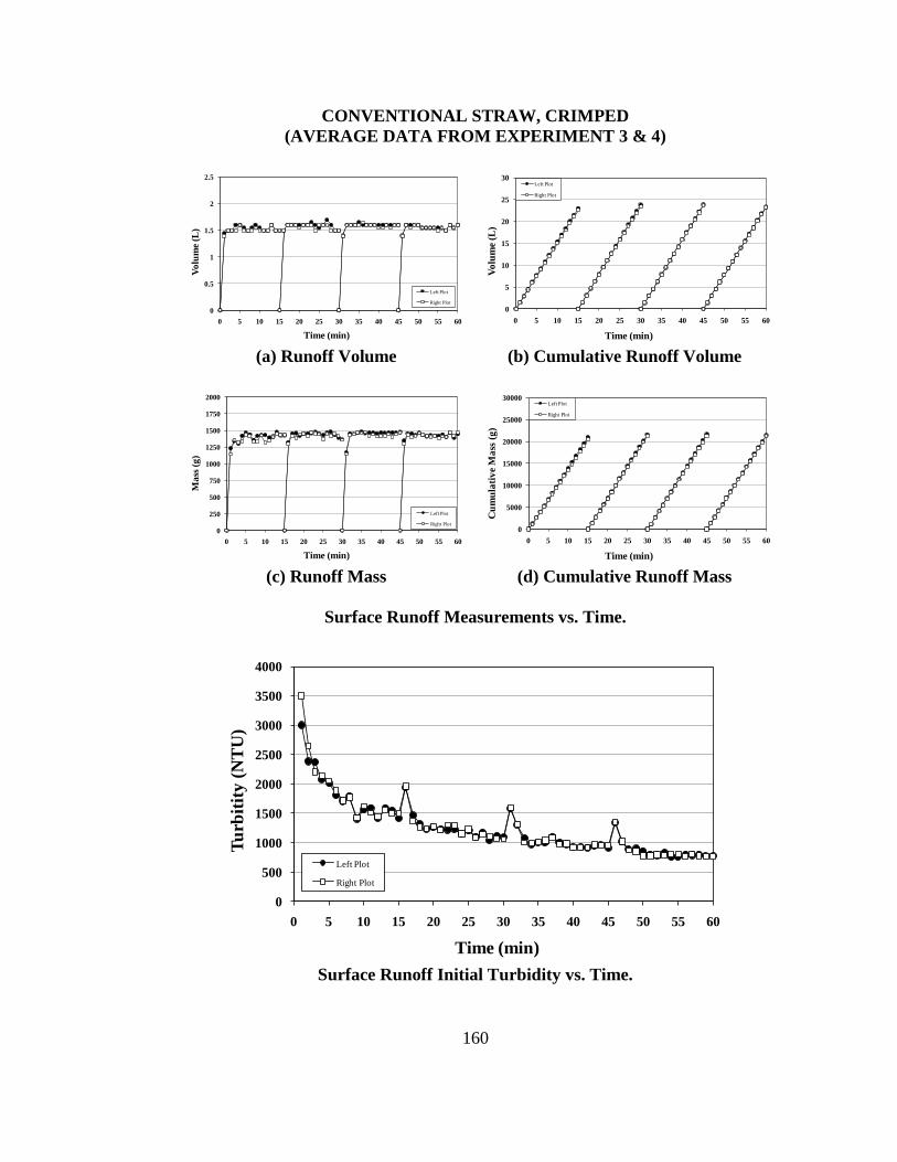
160
CONVENTIONAL STRAW, CRIMPED
(AVERAGE DATA FROM EXPERIMENT 3 & 4)
(a) Runoff Volume (b) Cumulative Runoff Volume
(c) Runoff Mass (d) Cumulative Runoff Mass
Surface Runoff Measurements vs. Time.
Surface Runoff Initial Turbidity vs. Time.
0
0.5
1
1.5
2
2.5
0 5 10 15 20 25 30 35 40 45 50 55 60
Vo
lum
e (L
)
Time (min)
Left Plot
Right Plot
0
5
10
15
20
25
30
0 5 10 15 20 25 30 35 40 45 50 55 60
Vo
lum
e (L
)
Time (min)
Left Plot
Right Plot
0
250
500
750
1000
1250
1500
1750
2000
0 5 10 15 20 25 30 35 40 45 50 55 60
Ma
ss (
g)
Time (min)
Left Plot
Right Plot
0
5000
10000
15000
20000
25000
30000
0 5 10 15 20 25 30 35 40 45 50 55 60
Cu
mu
lati
ve
Ma
ss (
g)
Time (min)
Left Plot
Right Plot
0
500
1000
1500
2000
2500
3000
3500
4000
0 5 10 15 20 25 30 35 40 45 50 55 60
Tu
rbit
ity
(N
TU
)
Time (min)
Left Plot
Right Plot

161
(a) Turbidity vs. Time at 5 Minutes (b) Turbidity vs. Time at 10 Minutes
Turbidity vs. Time for Samples Collected at 5 and 10 Minutes.
(a) Soil Loss vs. Time (b) Cumulative Soil Loss vs. Time
Soil Loss and Cumulative Soil Loss vs. Time.
Conventional Straw, Crimped, Post-Experimentation.
0
500
1000
1500
2000
2500
3000
0 50 100 150 200
Tu
rbid
ity
(N
TU
)
Time (sec)
TR1 - Left
TR1 - Right
TR2 - Left
TR2 - Right
TR3 - Left
TR3 - Right
TR4 - Left
TR4 - Right
0
200
400
600
800
1000
1200
1400
1600
1800
0 50 100 150 200
Tu
rbid
ity
(N
TU
)
Time (sec)
TR1 - Left
TR1 - Right
TR2 - Left
TR2 - Right
TR3 - Left
TR3 - Right
TR4 - Left
TR4 - Right
0
20
40
60
80
100
0 5 10 15 20 25 30 35 40 45 50 55 60
So
il L
oss
(g
)
Time (min)
Left Plot
Right Plot
0
50
100
150
200
250
0 5 10 15 20 25 30 35 40 45 50 55 60
Cu
mu
lati
ve
So
il L
oss
(g
)
Time (min)
Left Plot
Right Plot
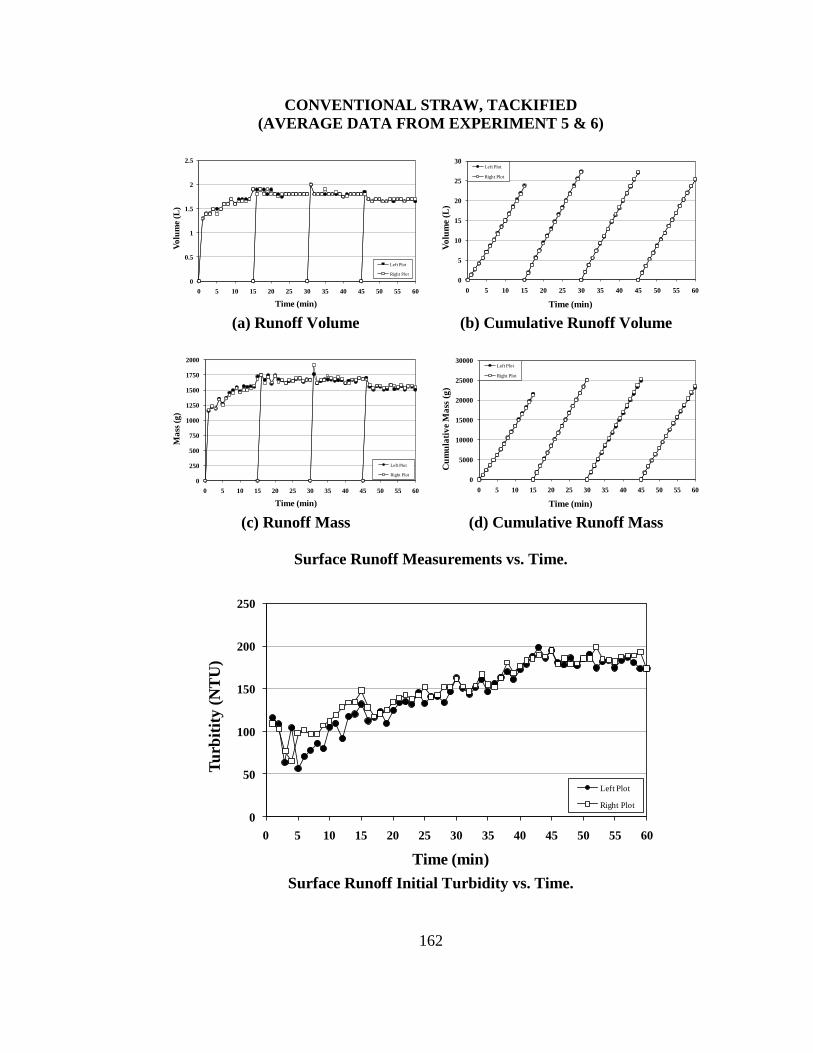
162
CONVENTIONAL STRAW, TACKIFIED
(AVERAGE DATA FROM EXPERIMENT 5 & 6)
(a) Runoff Volume (b) Cumulative Runoff Volume
(c) Runoff Mass (d) Cumulative Runoff Mass
Surface Runoff Measurements vs. Time.
Surface Runoff Initial Turbidity vs. Time.
0
0.5
1
1.5
2
2.5
0 5 10 15 20 25 30 35 40 45 50 55 60
Vo
lum
e (L
)
Time (min)
Left Plot
Right Plot
0
5
10
15
20
25
30
0 5 10 15 20 25 30 35 40 45 50 55 60
Vo
lum
e (L
)
Time (min)
Left Plot
Right Plot
0
250
500
750
1000
1250
1500
1750
2000
0 5 10 15 20 25 30 35 40 45 50 55 60
Ma
ss (
g)
Time (min)
Left Plot
Right Plot
0
5000
10000
15000
20000
25000
30000
0 5 10 15 20 25 30 35 40 45 50 55 60
Cu
mu
lati
ve
Ma
ss (
g)
Time (min)
Left Plot
Right Plot
0
50
100
150
200
250
0 5 10 15 20 25 30 35 40 45 50 55 60
Tu
rbit
ity
(N
TU
)
Time (min)
Left Plot
Right Plot

163
(a) Turbidity vs. Time at 5 Minutes (b) Turbidity vs. Time at 10 Minutes
Turbidity vs. Time for Samples Collected at 5 and 10 Minutes.
(a) Soil Loss vs. Time (b) Cumulative Soil Loss vs. Time
Soil Loss and Cumulative Soil Loss vs. Time.
Conventional Straw w/Tackifier, Post-Experimentation.
0
100
200
300
400
500
0 50 100 150 200
Tu
rbid
ity
(N
TU
)
Time (sec)
TR1 - Left
TR1 - Right
TR2 - Left
TR2 - Right
TR3 - Left
TR3 - Right
TR4 - Left
TR4 - Right
0
100
200
300
400
500
0 50 100 150 200
Tu
rbid
ity
(N
TU
)
Time (sec)
TR1 - Left
TR1 - Right
TR2 - Left
TR2 - Right
TR3 - Left
TR3 - Right
TR4 - Left
TR4 - Right
0
10
20
30
40
50
0 5 10 15 20 25 30 35 40 45 50 55 60
So
il L
oss
(g
)
Time (min)
Left Plot
Right Plot
0
10
20
30
40
50
0 5 10 15 20 25 30 35 40 45 50 55 60
Cu
mu
lati
ve
So
il L
oss
(g
)
Time (min)
Left Plot
Right Plot

164
EXCEL® FIBERMULCH II
(AVERAGE DATA FROM EXPERIMENT 7 & 8)
(a) Runoff Volume (b) Cumulative Runoff Volume
(c) Runoff Mass (d) Cumulative Runoff Mass
Surface Runoff Measurements vs. Time.
Surface Runoff Initial Turbidity vs. Time.
0
0.5
1
1.5
2
2.5
0 5 10 15 20 25 30 35 40 45 50 55 60
Vo
lum
e (L
)
Time (min)
Left Plot
Right Plot
0
5
10
15
20
25
30
0 5 10 15 20 25 30 35 40 45 50 55 60
Vo
lum
e (L
)
Time (min)
Left Plot
Right Plot
0
250
500
750
1000
1250
1500
1750
2000
0 5 10 15 20 25 30 35 40 45 50 55 60
Ma
ss (
g)
Time (min)
Left Plot
Right Plot
0
5000
10000
15000
20000
25000
30000
0 5 10 15 20 25 30 35 40 45 50 55 60
Cu
mu
lati
ve
Ma
ss (
g)
Time (min)
Left Plot
Right Plot
0
500
1000
1500
2000
2500
0 5 10 15 20 25 30 35 40 45 50 55 60
Tu
rbit
ity
(N
TU
)
Time (min)
Left Plot
Right Plot

165
(a) Turbidity vs. Time at 5 Minutes (b) Turbidity vs. Time at 10 Minutes
Turbidity vs. Time for Samples Collected at 5 and 10 Minutes.
(a) Soil Loss vs. Time (b) Cumulative Soil Loss vs. Time
Soil Loss and Cumulative Soil Loss vs. Time.
Excel® Fibermulch II, Post-Experimentation.
0
2000
4000
6000
8000
10000
0 50 100 150 200
Tu
rbid
ity
(N
TU
)
Time (sec)
TR1 - Left
TR1 - Right
TR2 - Left
TR2 - Right
TR3 - Left
TR3 - Right
TR4 - Left
TR4 - Right
0
2000
4000
6000
8000
10000
0 50 100 150 200
Tu
rbid
ity
(N
TU
)
Time (sec)
TR1 - Left
TR1 - Right
TR2 - Left
TR2 - Right
TR3 - Left
TR3 - Right
TR4 - Left
TR4 - Right
0
50
100
150
200
250
0 5 10 15 20 25 30 35 40 45 50 55 60
So
il L
oss
(g
)
Time (min)
Left Plot
Right Plot
0
100
200
300
400
500
600
700
800
900
0 5 10 15 20 25 30 35 40 45 50 55 60
Cu
mu
lati
ve
So
il L
oss
(g
)
Time (min)
Left Plot
Right Plot

166
GEOSKIN®
(AVERAGE DATA FROM EXPERIMENT 9 & 10)
(a) Runoff Volume (b) Cumulative Runoff Volume
(c) Runoff Mass (d) Cumulative Runoff Mass
Surface Runoff Measurements vs. Time.
Surface Runoff Initial Turbidity vs. Time.
0
0.5
1
1.5
2
2.5
0 5 10 15 20 25 30 35 40 45 50 55 60
Vo
lum
e (L
)
Time (min)
Left Plot
Right Plot
0
5
10
15
20
25
30
0 5 10 15 20 25 30 35 40 45 50 55 60
Vo
lum
e (L
)
Time (min)
Left Plot
Right Plot
0
250
500
750
1000
1250
1500
1750
2000
0 5 10 15 20 25 30 35 40 45 50 55 60
Ma
ss (
g)
Time (min)
Left Plot
Right Plot
0
5000
10000
15000
20000
25000
30000
0 5 10 15 20 25 30 35 40 45 50 55 60
Cu
mu
lati
ve
Ma
ss (
g)
Time (min)
Left Plot
Right Plot
0
100
200
300
400
500
600
700
800
900
1000
0 5 10 15 20 25 30 35 40 45 50 55 60
Tu
rbit
ity
(N
TU
)
Time (min)
Left Plot
Right Plot
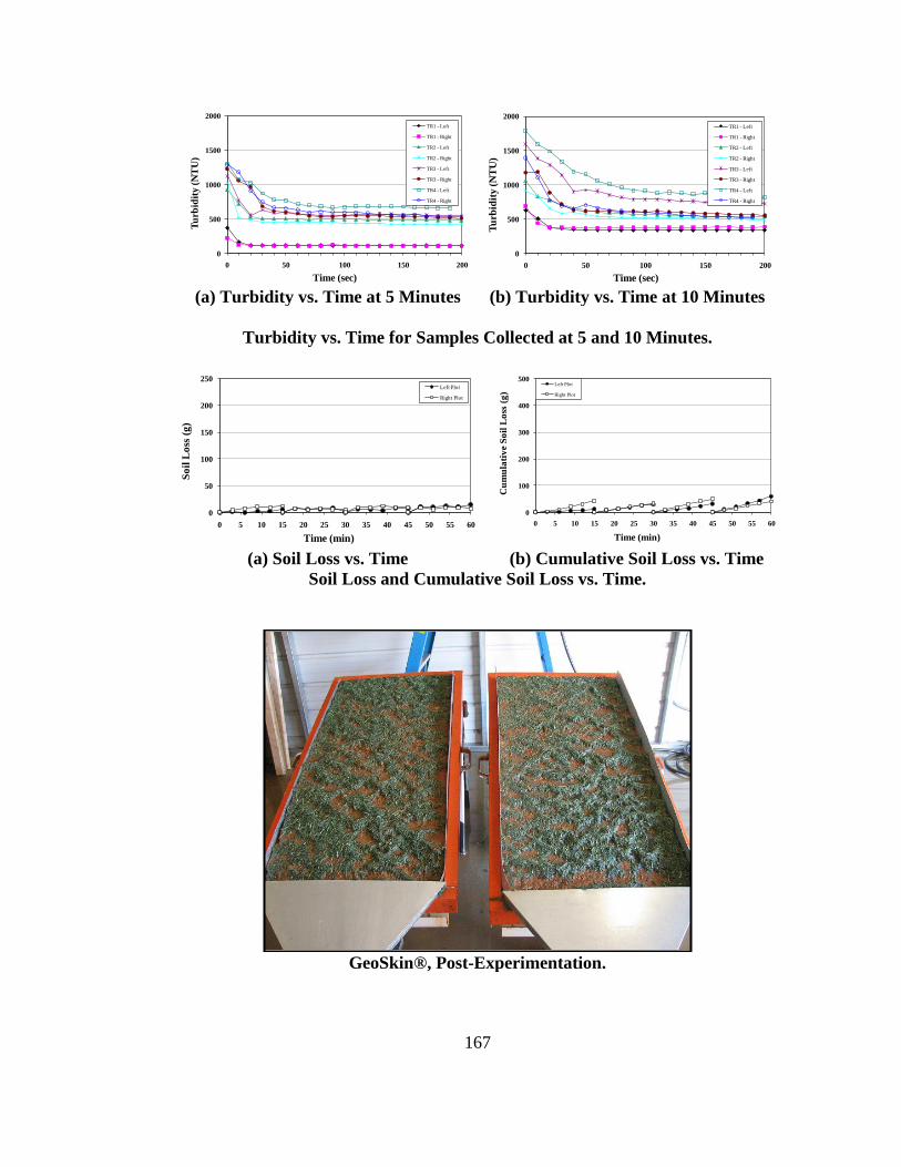
167
(a) Turbidity vs. Time at 5 Minutes (b) Turbidity vs. Time at 10 Minutes
Turbidity vs. Time for Samples Collected at 5 and 10 Minutes.
(a) Soil Loss vs. Time (b) Cumulative Soil Loss vs. Time
Soil Loss and Cumulative Soil Loss vs. Time.
GeoSkin®, Post-Experimentation.
0
500
1000
1500
2000
0 50 100 150 200
Tu
rbid
ity
(N
TU
)
Time (sec)
TR1 - Left
TR1 - Right
TR2 - Left
TR2 - Right
TR3 - Left
TR3 - Right
TR4 - Left
TR4 - Right
0
500
1000
1500
2000
0 50 100 150 200
Tu
rbid
ity
(N
TU
)
Time (sec)
TR1 - Left
TR1 - Right
TR2 - Left
TR2 - Right
TR3 - Left
TR3 - Right
TR4 - Left
TR4 - Right
0
50
100
150
200
250
0 5 10 15 20 25 30 35 40 45 50 55 60
So
il L
oss
(g
)
Time (min)
Left Plot
Right Plot
0
100
200
300
400
500
0 5 10 15 20 25 30 35 40 45 50 55 60
Cu
mu
lati
ve
So
il L
oss
(g
)
Time (min)
Left Plot
Right Plot

168
HYDRACX2®
(AVERAGE DATA FROM EXPERIMENT 11 & 12)
(a) Runoff Volume (b) Cumulative Runoff Volume
(c) Runoff Mass (d) Cumulative Runoff Mass
Surface Runoff Measurements vs. Time.
Surface Runoff Initial Turbidity vs. Time.
0
0.5
1
1.5
2
2.5
0 5 10 15 20 25 30 35 40 45 50 55 60
Vo
lum
e (L
)
Time (min)
Left Plot
Right Plot
0
5
10
15
20
25
30
0 5 10 15 20 25 30 35 40 45 50 55 60
Vo
lum
e (L
)
Time (min)
Left Plot
Right Plot
0
250
500
750
1000
1250
1500
1750
2000
0 5 10 15 20 25 30 35 40 45 50 55 60
Ma
ss (
g)
Time (min)
Left Plot
Right Plot
0
5000
10000
15000
20000
25000
30000
0 5 10 15 20 25 30 35 40 45 50 55 60
Cu
mu
lati
ve
Ma
ss (
g)
Time (min)
Left Plot
Right Plot
0
50
100
150
200
250
300
350
400
450
500
0 5 10 15 20 25 30 35 40 45 50 55 60
Tu
rbit
ity
(N
TU
)
Time (min)
Left Plot
Right Plot

169
(a) Turbidity vs. Time at 5 Minutes (b) Turbidity vs. Time at 10 Minutes
Turbidity vs. Time for Samples Collected at 5 and 10 Minutes.
(a) Soil Loss vs. Time (b) Cumulative Soil Loss vs. Time
Soil Loss and Cumulative Soil Loss vs. Time.
HydraCX
2®, Post-Experimentation.
0
200
400
600
800
1000
0 50 100 150 200
Tu
rbid
ity
(N
TU
)
Time (sec)
TR1 - Left
TR1 - Right
TR2 - Left
TR2 - Right
TR3 - Left
TR3 - Right
TR4 - Left
TR4 - Right
0
200
400
600
800
1000
0 50 100 150 200
Tu
rbid
ity
(N
TU
)
Time (sec)
TR1 - Left
TR1 - Right
TR2 - Left
TR2 - Right
TR3 - Left
TR3 - Right
TR4 - Left
TR4 - Right
0
50
100
150
200
250
0 5 10 15 20 25 30 35 40 45 50 55 60
So
il L
oss
(g
)
Time (min)
Left Plot
Right Plot
0
50
100
150
200
250
0 5 10 15 20 25 30 35 40 45 50 55 60
Cu
mu
lati
ve
So
il L
oss
(g
)
Time (min)
Left Plot
Right Plot
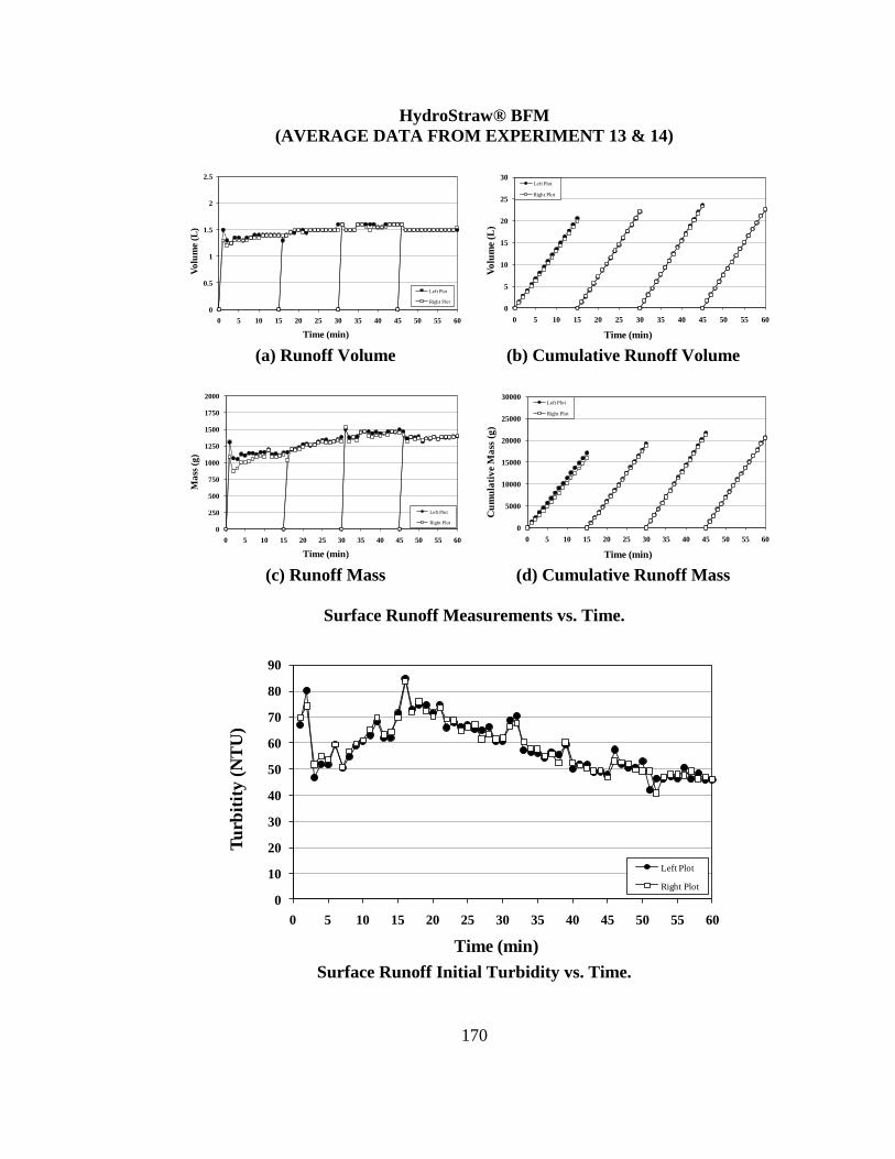
170
HydroStraw® BFM
(AVERAGE DATA FROM EXPERIMENT 13 & 14)
(a) Runoff Volume (b) Cumulative Runoff Volume
(c) Runoff Mass (d) Cumulative Runoff Mass
Surface Runoff Measurements vs. Time.
Surface Runoff Initial Turbidity vs. Time.
0
0.5
1
1.5
2
2.5
0 5 10 15 20 25 30 35 40 45 50 55 60
Vo
lum
e (L
)
Time (min)
Left Plot
Right Plot
0
5
10
15
20
25
30
0 5 10 15 20 25 30 35 40 45 50 55 60
Vo
lum
e (L
)
Time (min)
Left Plot
Right Plot
0
250
500
750
1000
1250
1500
1750
2000
0 5 10 15 20 25 30 35 40 45 50 55 60
Ma
ss (
g)
Time (min)
Left Plot
Right Plot
0
5000
10000
15000
20000
25000
30000
0 5 10 15 20 25 30 35 40 45 50 55 60
Cu
mu
lati
ve
Ma
ss (
g)
Time (min)
Left Plot
Right Plot
0
10
20
30
40
50
60
70
80
90
0 5 10 15 20 25 30 35 40 45 50 55 60
Tu
rbit
ity
(N
TU
)
Time (min)
Left Plot
Right Plot

171
(a) Turbidity vs. Time at 5 Minutes (b) Turbidity vs. Time at 10 Minutes
Turbidity vs. Time for Samples Collected at 5 and 10 Minutes.
(a) Soil Loss vs. Time (b) Cumulative Soil Loss vs. Time
Soil Loss and Cumulative Soil Loss vs. Time.
HydroStraw® BFM, Post-Experimentation.
0
50
100
150
200
250
0 50 100 150 200
Tu
rbid
ity
(N
TU
)
Time (sec)
TR1 - Left
TR1 - Right
TR2 - Left
TR2 - Right
TR3 - Left
TR3 - Right
TR4 - Left
TR4 - Right
0
50
100
150
200
250
0 50 100 150 200
Tu
rbid
ity
(N
TU
)
Time (sec)
TR1 - Left
TR1 - Right
TR2 - Left
TR2 - Right
TR3 - Left
TR3 - Right
TR4 - Left
TR4 - Right
0
10
20
30
40
50
0 5 10 15 20 25 30 35 40 45 50 55 60
So
il L
oss
(g
)
Time (min)
Left Plot
Right Plot
0
10
20
30
40
50
0 5 10 15 20 25 30 35 40 45 50 55 60
Cu
mu
lati
ve
So
il L
oss
(g
)
Time (min)
Left Plot
Right Plot

172
Appendix 7 Statistical Analysis

173
Tukey-Kramer Multiple Comparisons on Average Initial Turbidity [Test 1]
Comparison µi - µj CI [LB] CI [UB] Significantly Different
Control vs. GeoSkin 6640 6351 6929 Yes
Control vs. Straw, Crimped 5155 4866 5444 Yes
Control vs.HydraCX2
6806 6518 7095 Yes
Control vs. Excel Fibermulch II 5777 5489 6066 Yes
Control vs. HydroStraw BFM 6914 6625 7203 Yes
Control vs. Straw, Tackified 6873 6584 7162 Yes
GeoSkin vs. Straw, Crimped 1485 1197 1774 Yes
GeoSkin vs. HydraCX2
166 -123 455 No
GeoSkin vs. Excel Fibermulch II 863 574 1152 Yes
GeoSkin vs. HydroStraw BFM 274 -15 563 No
GeoSkin vs. Straw, Tackified 232 -56 521 No
Straw, Crimped vs. HydraCX2
1652 1363 1940 Yes
Straw, Crimped vs. Excel Fibermulch II 623 334 911 Yes
Straw, Crimped vs. HydroStraw BFM 1759 1470 2048 Yes
Straw, Crimped vs. Straw, Tackified 1718 1429 2007 Yes
HydraCX2 vs. Excel Fibermulch II 1029 740 1318 Yes
HydraCX2 vs. HydroStraw BFM 108 -181 397 No
HydraCX2 vs. Straw, Tackified 66 -222 355 No
Excel Fibermulch II vs. HydroStraw BFM 1137 848 1426 Yes
Excel Fibermulch II vs. Straw, Tackified 1095 807 1384 Yes
HydroStraw BFM vs. Straw, Tackified 41 -247 330 No Notes: [LB] signifies lower bound of confidence interval
[UB] signifies upper bound of confidence interval
qcrit = 4.28
Tukey-Kramer Multiple Comparisons on Average Initial Turbidity [Test 2]
Comparison µi - µj CI [LB] CI [UB] Significantly Different
Control vs. GeoSkin 5541 5391 5691 Yes
Control vs. Straw, Crimped 4795 4645 4945 Yes
Control vs.HydraCX2
5757 5607 5907 Yes
Control vs. Excel Fibermulch II 5267 5117 5416 Yes
Control vs. HydroStraw BFM 5983 5833 6133 Yes
Control vs. Straw, Tackified 5916 5766 6065 Yes
GeoSkin vs. Straw, Crimped 746 596 896 Yes
GeoSkin vs. HydraCX2
216 66 365 Yes
GeoSkin vs. Excel Fibermulch II 275 125 424 Yes
GeoSkin vs. HydroStraw BFM 441 292 591 Yes
GeoSkin vs. Straw, Tackified 374 224 524 Yes
Straw, Crimped vs. HydraCX2
962 812 1112 Yes
Straw, Crimped vs. Excel Fibermulch II 471 322 621 Yes
Straw, Crimped vs. HydroStraw BFM 1188 1038 1337 Yes
Straw, Crimped vs. Straw, Tackified 1120 971 1270 Yes
HydraCX2 vs. Excel Fibermulch II 490 340 640 Yes
HydraCX2 vs. HydroStraw BFM 226 76 376 Yes
HydraCX2 vs. Straw, Tackified 159 9 309 Yes
Excel Fibermulch II vs. HydroStraw BFM 716 566 866 Yes
Excel Fibermulch II vs. Straw, Tackified 649 499 799 Yes
HydroStraw BFM vs. Straw, Tackified 67 -83 217 No Notes: [LB] signifies lower bound of confidence interval
[UB] signifies upper bound of confidence interval
qcrit = 4.28

174
Tukey-Kramer Multiple Comparisons on Average Initial Turbidity [Test 3]
Comparison µi - µj CI [LB] CI [UB] Significantly Different
Control vs. GeoSkin 5427 5301 5554 Yes
Control vs. Straw, Crimped 4880 4753 5007 Yes
Control vs.HydraCX2
5616 5490 5743 Yes
Control vs. Excel Fibermulch II 5081 4954 5207 Yes
Control vs. HydroStraw BFM 5878 5751 6004 Yes
Control vs. Straw, Tackified 5764 5637 5890 Yes
GeoSkin vs. Straw, Crimped 547 421 674 Yes
GeoSkin vs. HydraCX2
189 63 316 Yes
GeoSkin vs. Excel Fibermulch II 347 220 473 Yes
GeoSkin vs. HydroStraw BFM 450 324 577 Yes
GeoSkin vs. Straw, Tackified 336 210 463 Yes
Straw, Crimped vs. HydraCX2
736 610 863 Yes
Straw, Crimped vs. Excel Fibermulch II 200 74 327 Yes
Straw, Crimped vs. HydroStraw BFM 998 871 1124 Yes
Straw, Crimped vs. Straw, Tackified 884 757 1010 Yes
HydraCX2 vs. Excel Fibermulch II 536 409 663 Yes
HydraCX2 vs. HydroStraw BFM 261 135 388 Yes
HydraCX2 vs. Straw, Tackified 147 21 274 Yes
Excel Fibermulch II vs. HydroStraw BFM 797 671 924 Yes
Excel Fibermulch II vs. Straw, Tackified 683 557 810 Yes
HydroStraw BFM vs. Straw, Tackified 114 -13 241 No Notes: [LB] signifies lower bound of confidence interval
[UB] signifies upper bound of confidence interval
qcrit = 4.28
Tukey-Kramer Multiple Comparisons on Average Initial Turbidity [Test 4]
Comparison µi - µj CI [LB] CI [UB] Significantly Different
Control vs. GeoSkin 4628 4516 4741 Yes
Control vs. Straw, Crimped 4450 4338 4562 Yes
Control vs.HydraCX2
4953 4840 5065 Yes
Control vs. Excel Fibermulch II 4393 4280 4505 Yes
Control vs. HydroStraw BFM 5230 5118 5343 Yes
Control vs. Straw, Tackified 5096 4983 5208 Yes
GeoSkin vs. Straw, Crimped 178 66 291 Yes
GeoSkin vs. HydraCX2
325 212 437 Yes
GeoSkin vs. Excel Fibermulch II 236 123 348 Yes
GeoSkin vs. HydroStraw BFM 602 490 715 Yes
GeoSkin vs. Straw, Tackified 468 355 580 Yes
Straw, Crimped vs. HydraCX2
503 390 615 Yes
Straw, Crimped vs. Excel Fibermulch II 57 -55 170 No
Straw, Crimped vs. HydroStraw BFM 780 668 893 Yes
Straw, Crimped vs. Straw, Tackified 646 533 758 Yes
HydraCX2 vs. Excel Fibermulch II 560 448 673 Yes
HydraCX2 vs. HydroStraw BFM 278 165 390 Yes
HydraCX2 vs. Straw, Tackified 143 31 255 Yes
Excel Fibermulch II vs. HydroStraw BFM 838 725 950 Yes
Excel Fibermulch II vs. Straw, Tackified 703 591 816 Yes
HydroStraw BFM vs. Straw, Tackified 135 22 247 Yes Notes: [LB] signifies lower bound of confidence interval
[UB] signifies upper bound of confidence interval
qcrit = 4.28

175
Tukey-Kramer Multiple Comparisons on Average Soil Loss [Test 1]
Comparison µi - µj CI [LB] CI [UB] Significantly Different
Control vs. GeoSkin 17158 15582 18733 Yes
Control vs. Straw, Crimped 16656 15080 18231 Yes
Control vs.HydraCX2
17256 15680 18832 Yes
Control vs. Excel Fibermulch II 16461 14886 18037 Yes
Control vs. HydroStraw BFM 17332 15756 18908 Yes
Control vs. Straw, Tackified 17158 15582 18734 Yes
GeoSkin vs. Straw, Crimped 502 -1074 2078 No
GeoSkin vs. HydraCX2
98 -1477 1674 No
GeoSkin vs. Excel Fibermulch II 696 -880 2272 No
GeoSkin vs. HydroStraw BFM 174 -1401 1750 No
GeoSkin vs. Straw, Tackified 0 -1575 1576 No
Straw, Crimped vs. HydraCX2
601 -975 2176 No
Straw, Crimped vs. Excel Fibermulch II 194 -1382 1770 No
Straw, Crimped vs. HydroStraw BFM 676 -899 2252 No
Straw, Crimped vs. Straw, Tackified 502 -1073 2078 No
HydraCX2 vs. Excel Fibermulch II 795 -781 2370 No
HydraCX2 vs. HydroStraw BFM 76 -1500 1652 No
HydraCX2 vs. Straw, Tackified 98 -1478 1674 No
Excel Fibermulch II vs. HydroStraw BFM 871 -705 2446 No
Excel Fibermulch II vs. Straw, Tackified 697 -879 2272 No
HydroStraw BFM vs. Straw, Tackified 174 -1402 1750 No Notes: [LB] signifies lower bound of confidence interval
[UB] signifies upper bound of confidence interval
qcrit = 4.49
Tukey-Kramer Multiple Comparisons on Average Soil Loss [Test 2]
Comparison µi - µj CI [LB] CI [UB] Significantly Different
Control vs. GeoSkin 7347 7252 7442 Yes
Control vs. Straw, Crimped 7211 7115 7306 Yes
Control vs.HydraCX2
7450 7355 7545 Yes
Control vs. Excel Fibermulch II 6989 6894 7084 Yes
Control vs. HydroStraw BFM 7506 7411 7602 Yes
Control vs. Straw, Tackified 7385 7290 7481 Yes
GeoSkin vs. Straw, Crimped 137 42 232 Yes
GeoSkin vs. HydraCX2
103 8 198 Yes
GeoSkin vs. Excel Fibermulch II 358 263 453 Yes
GeoSkin vs. HydroStraw BFM 159 64 254 Yes
GeoSkin vs. Straw, Tackified 38 -57 133 No
Straw, Crimped vs. HydraCX2
240 145 335 Yes
Straw, Crimped vs. Excel Fibermulch II 221 126 316 Yes
Straw, Crimped vs. HydroStraw BFM 296 201 391 Yes
Straw, Crimped vs. Straw, Tackified 175 80 270 Yes
HydraCX2 vs. Excel Fibermulch II 461 366 556 Yes
HydraCX2 vs. HydroStraw BFM 56 -39 151 No
HydraCX2 vs. Straw, Tackified 65 -30 160 No
Excel Fibermulch II vs. HydroStraw BFM 517 422 612 Yes
Excel Fibermulch II vs. Straw, Tackified 396 301 491 Yes
HydroStraw BFM vs. Straw, Tackified 121 26 216 Yes Notes: [LB] signifies lower bound of confidence interval
[UB] signifies upper bound of confidence interval
qcrit = 4.49

176
Tukey-Kramer Multiple Comparisons on Average Soil Loss [Test 3]
Comparison µi - µj CI [LB] CI [UB] Significantly Different
Control vs. GeoSkin 6859 6764 6953 Yes
Control vs. Straw, Crimped 6869 6774 6964 Yes
Control vs.HydraCX2
7013 6918 7108 Yes
Control vs. Excel Fibermulch II 6604 6509 6699 Yes
Control vs. HydroStraw BFM 7098 7003 7193 Yes
Control vs. Straw, Tackified 7011 6916 7106 Yes
GeoSkin vs. Straw, Crimped 10 -85 105 No
GeoSkin vs. HydraCX2
155 60 249 Yes
GeoSkin vs. Excel Fibermulch II 254 160 349 Yes
GeoSkin vs. HydroStraw BFM 240 145 335 Yes
GeoSkin vs. Straw, Tackified 152 57 247 Yes
Straw, Crimped vs. HydraCX2
144 50 239 Yes
Straw, Crimped vs. Excel Fibermulch II 265 170 360 Yes
Straw, Crimped vs. HydroStraw BFM 230 135 324 Yes
Straw, Crimped vs. Straw, Tackified 142 47 237 Yes
HydraCX2 vs. Excel Fibermulch II 409 314 504 Yes
HydraCX2 vs. HydroStraw BFM 85 -10 180 No
HydraCX2 vs. Straw, Tackified 2 -92 97 No
Excel Fibermulch II vs. HydroStraw BFM 494 399 589 Yes
Excel Fibermulch II vs. Straw, Tackified 407 312 501 Yes
HydroStraw BFM vs. Straw, Tackified 88 -7 182 No Notes: [LB] signifies lower bound of confidence interval
[UB] signifies upper bound of confidence interval
qcrit = 4.49
Tukey-Kramer Multiple Comparisons on Average Soil Loss [Test 4]
Comparison µi - µj CI [LB] CI [UB] Significantly Different
Control vs. GeoSkin 5767 5692 5842 Yes
Control vs. Straw, Crimped 5947 5872 6022 Yes
Control vs.HydraCX2
5980 5905 6055 Yes
Control vs. Excel Fibermulch II 5689 5614 5765 Yes
Control vs. HydroStraw BFM 6097 6022 6172 Yes
Control vs. Straw, Tackified 6001 5926 6077 Yes
GeoSkin vs. Straw, Crimped 180 104 255 Yes
GeoSkin vs. HydraCX2
213 137 288 Yes
GeoSkin vs. Excel Fibermulch II 78 2 153 Yes
GeoSkin vs. HydroStraw BFM 330 255 405 Yes
GeoSkin vs. Straw, Tackified 234 159 310 Yes
Straw, Crimped vs. HydraCX2
33 -42 108 No
Straw, Crimped vs. Excel Fibermulch II 257 182 333 Yes
Straw, Crimped vs. HydroStraw BFM 150 75 226 Yes
Straw, Crimped vs. Straw, Tackified 55 -21 130 No
HydraCX2 vs. Excel Fibermulch II 290 215 366 Yes
HydraCX2 vs. HydroStraw BFM 117 42 193 Yes
HydraCX2 vs. Straw, Tackified 22 -54 97 No
Excel Fibermulch II vs. HydroStraw BFM 408 333 483 Yes
Excel Fibermulch II vs. Straw, Tackified 312 237 387 Yes
HydroStraw BFM vs. Straw, Tackified 96 20 171 Yes Notes: [LB] signifies lower bound of confidence interval
[UB] signifies upper bound of confidence interval
qcrit = 4.49
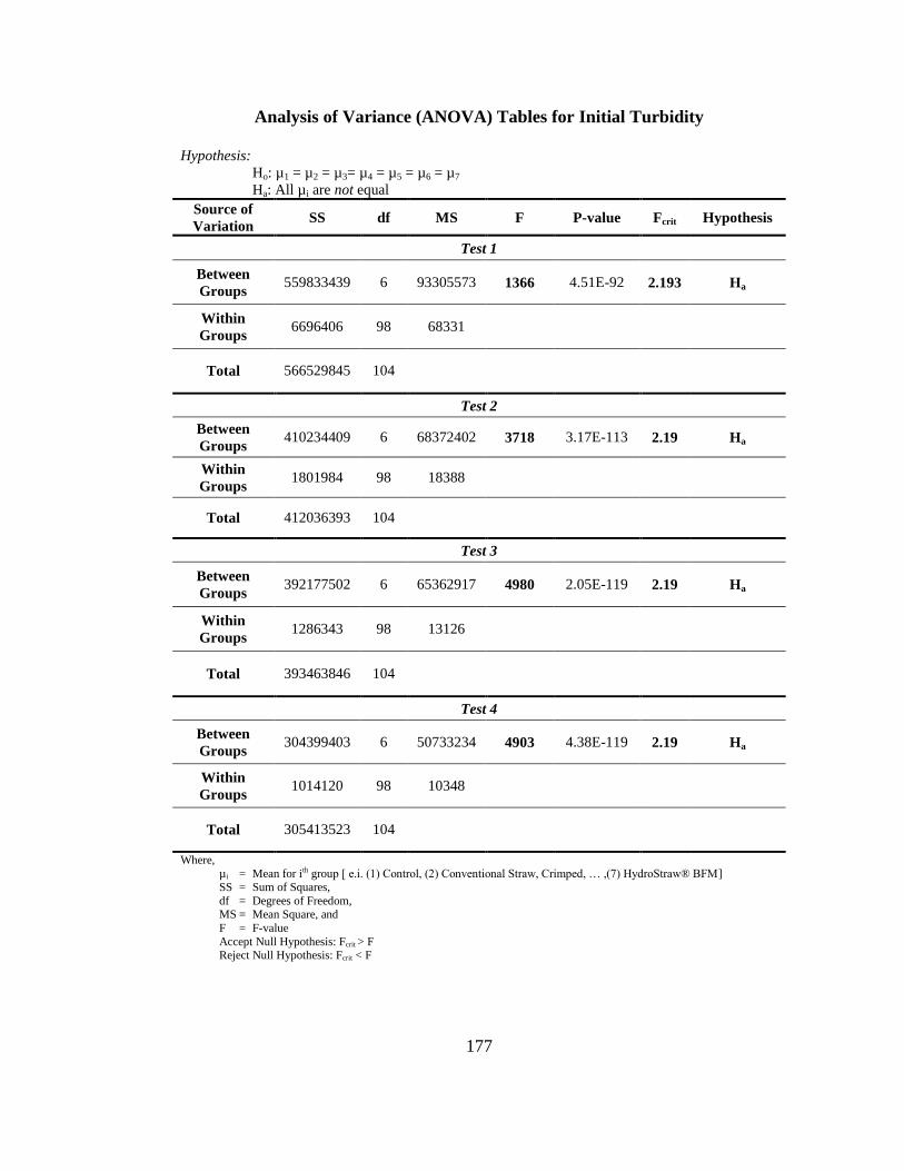
177
Analysis of Variance (ANOVA) Tables for Initial Turbidity
Hypothesis:
Ho: µ1 = µ2 = µ3= µ4 = µ5 = µ6 = µ7
Ha: All µi are not equal
Source of
Variation SS df MS F P-value Fcrit Hypothesis
Test 1
Between
Groups 559833439 6 93305573 1366 4.51E-92 2.193 Ha
Within
Groups 6696406 98 68331
Total 566529845 104
Test 2
Between
Groups 410234409 6 68372402 3718 3.17E-113 2.19 Ha
Within
Groups 1801984 98 18388
Total 412036393 104
Test 3
Between
Groups 392177502 6 65362917 4980 2.05E-119 2.19 Ha
Within
Groups 1286343 98 13126
Total 393463846 104
Test 4
Between
Groups 304399403 6 50733234 4903 4.38E-119 2.19 Ha
Within
Groups 1014120 98 10348
Total 305413523 104
Where,
µi = Mean for ith group [ e.i. (1) Control, (2) Conventional Straw, Crimped, … ,(7) HydroStraw® BFM] SS = Sum of Squares,
df = Degrees of Freedom, MS = Mean Square, and
F = F-value
Accept Null Hypothesis: Fcrit > F Reject Null Hypothesis: Fcrit < F

178
Analysis of Variance (ANOVA) Tables for Soil Loss
Hypothesis:
Ho: µ1 = µ2 = µ3= µ4 = µ5 = µ6 = µ7
Ha: All µi are not equal
Source of
Variation SS df MS F P-value Fcrit Hypothesis
Test 1
Between
Groups 49690005 6 8281667 13.45 3.93E-07 2.45 Ha
Within
Groups 17242822 28 615815
Total 66932826 34
Test 2
Between
Groups 9208386 6 1534731 684.4 5.06E-29 2.45 Ha
Within
Groups 62786 28 2242
Total 9271171 34
Test 3
Between
Groups 8213569 6 1368928 613.7 2.30E-28 2.45 Ha
Within
Groups 62462 28 2231
Total 8276031 34
Test 4
Between
Groups 6018693 6 1003116 713.6 2.83E-29 2.45 Ha
Within
Groups 39361 28 1406
Total 6058054 34
Where,
µi = Mean for ith group [ e.i. (1) Control, (2) Conventional Straw, Crimped, … ,(7) HydroStraw® BFM] SS = Sum of Squares,
df = Degrees of Freedom, MS = Mean Square, and
F = F-value
Accept Null Hypothesis: Fcrit > F Reject Null Hypothesis: Fcrit < F