evaluation of erosion control practices under large …
TRANSCRIPT

EVALUATION OF EROSION CONTROL PRACTICES
UNDER LARGE-SCALE RAINFALL SIMULATION
FOLLOWING ASTM D6459 STANDARD TEST METHODS
by
Brian Allen Faulkner
A thesis submitted to the Graduate Faculty of Auburn University
in partial fulfillment of the requirements for the Degree of
Master of Science
Auburn, Alabama May 2, 2020
Keywords: erosion, hydromulch, rainfall simulation, rolled erosion control blankets, stormwater, straw
Copyright 2020 by Brian Allen Faulkner
Approved by
Wesley N. Donald, Chair, Research Fellow IV Civil Engineering
Wesley C. Zech, Professor of Civil Engineering Xing Fang, Professor of Civil Engineering

ii
ABSTRACT
Land development and construction activities remove vegetative cover, exposing bare soil
to the erosive forces of rainfall. Stormwater causes dislodgement of soil particles through splash,
sheet, and rill erosion, resulting in soil particles being transported off-site causing pollution in local
water bodies and water conveyance systems. Erosion control practices are installed to minimize
the amount of erosion caused by erosive forces and to aid in the establishment of vegetation.
A rainfall simulator has been constructed at the Auburn University Erosion and Sediment
Control Test Facility (AU-ESCTF) following the ASTM D6459-19: The Standard Test Method
for Determination of Rolled Erosion Control Product (RECP) Performance in Protecting
Hillslopes from Rainfall Induced Erosion requirements. The rainfall simulator was constructed to
produce 2, 4, and 6 in. per hr (51, 102, and 152 mm per hr) rainfall intensities and has test plot
dimensions of 8 ft (2.4 m) wide by 40 ft (10.1 m) long on a 3H:1V slope. Each rainfall experiment
was an hour long with three sequential 20 minute rainfall intervals of increasing rainfall intensit ies
of 2, 4, and 6 in. per hr (51, 102, and 152 mm per hr). Calibration testing was performed on each
rainfall intensity to verify rainfall drop size distribution, intensity, and uniformity.
Bare soil control, loose straw, loose straw with tackifier, and crimped straw were evaluated
under rainfall simulation. The mulch practices and bare soil installations were evaluated under
initial and longevity performance testing. Following the completion of the straw mulch testing,
the soil type of the test slope was changed from a sandy loam to a loam soil, which better followed
the soil classification stated in ASTM D6459 standard. During this time, the test procedure was
altered to calculate the product C-factor. Three hydraulic mulches, three erosion control blankets,
and bare soil control tests were evaluated under the new test procedure. Following the completion

iii
of testing, the Revised Universal Soil Loss Equation (RUSLE) was used to calculate the product
C-factor from incremental rainfall depth and soil loss results.
Rainfall simulation tests performed on the sandy loam soil resulted in an average soil loss
of 738 lb. (335 kg) for bare soil, 143 lb. (64.9 kg) for loose straw, 97 lb. (44 kg) for loose straw,
and 169 lb. (76.6 kg) for crimped straw. Longevity testing was performed on the straw applications
following the initial product test resulting in a total soil loss 611 lb. (277 kg) for bare soil, 287 lb.
(130 kg) for loose straw, 131 lb. (59.4 kg) for loose straw with Tacking Agent 3, and 82 lb. (37.2
kg) for crimped straw. The initial and longevity test results were combined to determine which
practice reduced the overall soil loss. The loose straw with Tacking Agent 3 resulted in the highest
reduction in soil loss of 83%, which was closely followed by the crimped straw with an
improvement of 81%. This concluded that anchoring the straw mulch reduced the overall soil lose
better than the non-anchored straw applications.
Hydraulic mulches and erosion control blankets were evaluated on a loam soil with a new
test procedure that allows for the calculation of product C-factors. The loam soil had higher total
soil loss rates than the sandy loam soil with a total soil loss of 2,333 lb. (1,058 kg). The hydraulic
mulches resulted in C-factors of 0.55 for Eco-Fibre, 0.46 for Soil Cover, and 0.53 for Terra-Wood.
All three hydraulic mulches experienced high erosion rates caused by the product washing from
the test plot. Erosion control blankets tests resulted in C-factors of 0.05 for Curlex I, 0.14 for
S150, and 0.12 for ECX-2. The blankets resulted in lower C-factors than the hydraulic mulches.
The Curlex I blanket provided the best test plot coverage resulting in the lowest C-factor.

iv
ACKNOWLEDGEMENTS
The author would like to thank Dr. Wesley C. Zech for his encouragement to not only
pursue this graduate project, but also further guidance toward a specialized career goal. The author
would also like to extend thanks to Dr. Wesley N. Donald for his continuous assistance and
oversight in the greater development of the rainfall simulator and in myself as a graduate student.
Thank you to Dr. Xing Fang for guidance throughout the duration of the project, Mr. Guy Savage
for the extensive test facility management, and all undergraduate workers who aided in the
completion of testing. The author would also like to thank the Alabama Department of
Transportation for financially supporting this project. Lastly, the author would like to thank
Stephanie Faulkner and his parents Mike and Beth Faulkner for their love and support throughout
his graduate studies.

v
TABLE OF CONTENTS
ABSTRACT..................................................................................................................................... ii
ACKNOWLEDGEMENTS ............................................................................................................ iv
TABLE OF CONTENTS.................................................................................................................v
LIST OF TABLES ...........................................................................................................................x
LIST OF FIGURES ...................................................................................................................... xiii
1 CHAPTER 1: INTRODUCTION ............................................................................................ 1
1.1 Background ...................................................................................................................... 1
1.2 Rainfall Simulators........................................................................................................... 2
1.3 Research Objectives ......................................................................................................... 4
1.4 Organization of Thesis ..................................................................................................... 5
2 CHAPTER 2: LITERATURE REVIEW ................................................................................. 7
2.1 Rainfall Simulator Types ................................................................................................. 7
2.1.1 Drop Forming Rainfall Simulators ........................................................................... 7
2.1.2 Pressurized Rainfall Simulators ................................................................................ 7
2.2 CALIBRATION TESTING ............................................................................................. 8
2.2.1 Drop Size Distribution .............................................................................................. 8
2.3 Erosion Control Practices ............................................................................................... 12
2.3.1 Erosion Control Mulches ........................................................................................ 12
2.3.2 Rolled Erosion Control Products ............................................................................ 15
2.3.3 Erosion Control Practice Testing ............................................................................ 19
2.4 Revised Universal Soil Loss Equation ........................................................................... 30
2.4.1 Rainfall Erosivity Factor – R .................................................................................. 31

vi
2.4.2 Soil Erodibility Factor – K ...................................................................................... 32
2.4.3 Length Slope Steepness Factor – LS ....................................................................... 32
2.4.4 Cover Management Factor – C ............................................................................... 34
2.4.5 Support Practice Factor – P .................................................................................... 34
2.5 SUMMARY ................................................................................................................... 34
3 CHAPTER 3: METHODS AND PROCEDURES ............................................................... 40
3.1 INTRODUCTION.......................................................................................................... 40
3.2 CALIBRATION TESTING ........................................................................................... 41
3.2.1 Rainfall Uniformity and Intensity ........................................................................... 41
3.2.1 Drop Size Distribution ............................................................................................ 43
3.3 Validation Procedures .................................................................................................... 47
3.3.1 Slope Preparation .................................................................................................... 47
3.3.2 Drive Cylinder Compaction .................................................................................... 48
3.3.3 Turbidity.................................................................................................................. 52
3.3.4 Total Suspended Solids ........................................................................................... 53
3.4 Product Application........................................................................................................ 54
3.4.1 Loose Straw............................................................................................................. 54
3.4.2 Loose Straw with Tackifier..................................................................................... 55
3.4.3 Crimped Straw ........................................................................................................ 56
3.4.4 Hydraulic Erosion Control Products ....................................................................... 57
3.4.5 Rolled Erosion Control Products ............................................................................ 58
3.5 Rainfall Simulation test Procedure................................................................................. 60
3.5.1 Sandy Loam Test Procedure ................................................................................... 60

vii
3.5.2 Loam Test Procedure .............................................................................................. 61
3.6 SOIL ANALYSIS .......................................................................................................... 63
3.6.1 Dry Sieve Analysis – ASTM C136......................................................................... 64
3.6.2 Wet Sieve Analysis – ASTM C117 ........................................................................ 65
3.6.3 Proctor Compaction Test – ASTM D698 ............................................................... 66
3.6.4 Atterberg Test – ASTM D4318 .............................................................................. 68
3.6.5 Hydrometer Analysis – ASTM D7928 ................................................................... 70
3.7 REVISED UNIVERSAL SOIL LOSS EQUATION (RUSLE)..................................... 72
3.7.1 Soil Erodibility Factor – K-Factor .......................................................................... 73
3.7.2 Cover Management Factor – C-Factor.................................................................... 74
3.8 Summary ........................................................................................................................ 75
4 CHAPTER 4: RESULTS AND DISCUSSION .................................................................... 76
4.1 INTRODUCTION.......................................................................................................... 76
4.2 CALIBRATION RESULTS .......................................................................................... 76
4.2.1 Uniformity and Intensity ......................................................................................... 76
4.2.2 Drop Size Distribution ............................................................................................ 79
4.3 SOIL ANALYSIS RESULTS ........................................................................................ 81
4.3.1 Sandy Loam Soil ..................................................................................................... 81
4.3.2 Loam Soil ................................................................................................................ 84
4.3.3 Soil Summary.......................................................................................................... 87
4.4 STRAW MULCH TESTING......................................................................................... 87
4.4.1 Bare Soil Results ..................................................................................................... 87
4.4.2 Loose Straw Results................................................................................................ 89

viii
4.4.3 Loose Straw with Tacking Agent 3 ........................................................................ 91
4.4.4 Crimped Straw ........................................................................................................ 93
4.4.5 Straw Mulch Longevity Testing ............................................................................. 95
4.4.6 Straw Mulch Statistical Analysis .......................................................................... 103
4.4.7 Straw Summary..................................................................................................... 104
4.5 HYDRAULIC MULCH RESULTS............................................................................. 108
4.5.1 Loam Bare Soil Control ........................................................................................ 109
4.5.2 Eco-Fibre plus Tackifier ....................................................................................... 112
4.5.3 Soil Cover Wood Fiber with Tack ........................................................................ 119
4.5.4 Terra-Wood with Tacking Agent 3 ....................................................................... 124
4.5.5 Hydraulic Mulch Summary................................................................................... 129
4.6 EROSION CONTROL BLANKETS........................................................................... 132
4.6.1 Curlex I ................................................................................................................. 132
4.6.2 S150 ...................................................................................................................... 137
4.6.3 ECX-2 ................................................................................................................... 142
4.6.4 Erosion Control Blankets Summary ..................................................................... 148
4.6.5 Summary ............................................................................................................... 150
5 CHAPTER 5: CONCLUSION ............................................................................................ 152
5.1 INTRODUCTION........................................................................................................ 152
5.2 CALIBRATION TESTING ......................................................................................... 153
5.3 SANDY LOAM TESTING.......................................................................................... 153
5.4 LOAM SOIL TESTING............................................................................................... 155
5.4.1 Hydraulic Mulches ................................................................................................ 156

ix
5.4.2 Erosion Control Blankets ...................................................................................... 157
5.5 Summary ...................................................................................................................... 159
5.6 RECOMMENDATIONS FOR FURTURE RESEARCH ........................................... 161
REFERENCES ........................................................................................................................... 164
APPENDICES ............................................................................................................................ 168
APPENDIX A ............................................................................................................................. 169
APPENDIX B ............................................................................................................................. 176
APPENDIX C ............................................................................................................................. 188

x
LIST OF TABLES
TABLE 2.1: AL-SWCC Mulch Application Rates ..................................................................... 13
TABLE 2.2: HECP Classifications .............................................................................................. 15
TABLE 2.3: Erosion Control Product Classification (ALDOT 2018) ........................................ 16
TABLE 2.4: Faucette et al. 2007 ECB Results............................................................................ 27
TABLE 2.5: Sediment Yield Results (Benik 2003)..................................................................... 29
TABLE 2.6: Blown Mulch Summary .......................................................................................... 35
TABLE 2.7: Anchored Straw Summary ...................................................................................... 36
TABLE 2.8: Hydraulic Mulch Summary..................................................................................... 37
TABLE 2.9: Erosion Control Blanket Summary ......................................................................... 38
TABLE 4.1: Rainfall Intensity Results ........................................................................................ 77
TABLE 4.2: Rainfall Uniformity Results .................................................................................... 78
TABLE 4.3: Calibration Testing ANOVA Test Results ............................................................. 78
TABLE 4.4: Raindrop Fall Velocity............................................................................................ 79
TABLE 4.5: Rainfall Simulator Storm Energy............................................................................ 80
TABLE 4.6: Atterberg Classification .......................................................................................... 83
TABLE 4.7: Atterberg Soil Classification ................................................................................... 86
TABLE 4.8: Soil Analysis Summary........................................................................................... 87
TABLE 4.9: Bare Soil Control Results for Sandy Loam Soil ..................................................... 88
TABLE 4.10: Loose Straw Test Results ...................................................................................... 90
TABLE 4.11: Loose Straw with Tacking Agent 3 Results.......................................................... 92
TABLE 4.12: Crimped Straw Test Results.................................................................................. 94
TABLE 4.13: Loose Straw Longevity Soil Loss Results ............................................................ 97

xi
TABLE 4.14: Loose Straw with Tacking Agent 3 Longevity Results ........................................ 98
TABLE 4.15: Crimped Straw Longevity Results ...................................................................... 100
TABLE 4.16: Straw Mulch ANOVA Results............................................................................ 103
TABLE 4.17: Straw Mulch Hypothesis Test ............................................................................. 104
TABLE 4.18: Straw Mulch Soil Loss Results ........................................................................... 105
TABLE 4.19: Straw Mulch Longevity Soil Loss ...................................................................... 106
TABLE 4.20: Combined Straw Mulch Results ......................................................................... 108
TABLE 4.21: Loam Bare Soil Control Results ......................................................................... 109
TABLE 4.22: Bare Soil RUSLE Data ....................................................................................... 111
TABLE 4.23: K-factor Calculations .......................................................................................... 112
TABLE 4.24: Eco-Fibre plus Tackifier Test Results................................................................. 113
TABLE 4.25: Eco-Fibre RUSLE Calculations .......................................................................... 117
TABLE 4.26: Eco-Fibre plus Tackifier Hypothesis Test Results.............................................. 119
TABLE 4.27: Soil Cover Wood Fiber with Tack Test Results ................................................. 119
TABLE 4.28: Soil Cover RUSLE Equation .............................................................................. 123
TABLE 4.29: Soil Cover Hypothesis Test Results.................................................................... 124
TABLE 4.30: Terra-Wood with Tacking Agent 3 Test Results ................................................ 125
TABLE 4.31: Terra-Wood RUSLE Equation............................................................................ 128
TABLE 4.32: Terra-Wood Hypothesis Test Results ................................................................. 129
TABLE 4.33: Hydraulic Mulch Soil Loss Results .................................................................... 130
TABLE 4.34: Hydraulic Mulch C-Factor Results ..................................................................... 131
TABLE 4.35: Curlex I Test Results........................................................................................... 132
TABLE 4.36: Curlex I RUSLE Equation .................................................................................. 136

xii
TABLE 4.37: Curlex I Hypothesis Test Results........................................................................ 137
TABLE 4.38: S150 Test Results................................................................................................ 138
TABLE 4.39: S150 RUSLE Equation ....................................................................................... 141
TABLE 4.40: S150 Hypothesis Test Results............................................................................. 142
TABLE 4.41: ECX-2 Test Results............................................................................................. 143
TABLE 4.42: ECX-2 RUSLE Equation .................................................................................... 147
TABLE 4.43: ECX-2 Hypothesis Testing Results .................................................................... 148
TABLE 4.44: Erosion Control Blanket Soil Loss Summary ..................................................... 148
TABLE 4.45: ECB C-factor Results.......................................................................................... 149
TABLE 4.46: Rainfall Simulation Average Soil Loss Summary .............................................. 150

xiii
LIST OF FIGURES
FIGURE 2.1: P. Leonard Raindrop Analysis (Laws and Parsons 1943). ...................................... 9
FIGURE 2.2: Mass Ratio (Laws and Parsons, 1943). ................................................................. 10
FIGURE 2.3: RECP Anchoring Methods (ECTC 2014). ............................................................ 18
FIGURE 2.4: Downslope RECP Anchoring (ECTC 2014). ........................................................ 19
FIGURE 2.5: Drop Forming Rainfall Simulator (Khan et. al., 2016). ........................................ 20
FIGURE 2.6: Small Scale Rainfall Simulator at AU-ESCTF (Wilson et al. 2010). ................... 21
FIGURE 2.7: Foltz and Dooley (2003) Rainfall Simulator. ........................................................ 23
FIGURE 3.1: Rain Gauge Layout (ASTM 2019). ....................................................................... 41
FIGURE 3.2: Uniformity and Intensity Testing. ......................................................................... 42
FIGURE 3.3: Flour Pan Field Procedure. .................................................................................... 43
FIGURE 3.4: Flour Pan Lab Testing. .......................................................................................... 44
FIGURE 3.5: Raindrop Fall Velocity Chart (ASTM 2015). ....................................................... 45
FIGURE 3.6: Tilling Test Slope. ................................................................................................. 47
FIGURE 3.7: Slope Compaction. ................................................................................................ 48
FIGURE 3.8: Drive Cylinder Test Locations (Horne et al. 2017). .............................................. 49
FIGURE 3.9: Drive Cylinder Compaction Procedure. ................................................................ 50
FIGURE 3.10: Turbidity Lab Testing. ......................................................................................... 52
FIGURE 3.11: TSS Lab Testing. ................................................................................................. 54
FIGURE 3.12: Loose Straw Application. .................................................................................... 55
FIGURE 3.13: Tackifier Application. ......................................................................................... 56
FIGURE 3.14: Crimping Straw. .................................................................................................. 56
FIGURE 3.15: Hydroseeder used for Hydromulch Testing. ....................................................... 57

xiv
FIGURE 3.16: Hydraulic Mulch Application. ............................................................................. 58
FIGURE 3.17: Erosion Control Blanket Installation. .................................................................. 59
FIGURE 3.18: Water Runoff Analysis. ....................................................................................... 62
FIGURE 3.19: Soil Loss Analysis. .............................................................................................. 63
FIGURE 3.20: Dry Sieve Analysis. ............................................................................................. 65
FIGURE 3.21: Wet Sieve Analysis Testing. ............................................................................... 66
FIGURE 3.22: Proctor Compaction Pattern (ASTM 2012). ........................................................ 67
FIGURE 3.23: Proctor Compaction Procedure. .......................................................................... 68
FIGURE 3.24: Liquid Limit Testing. .......................................................................................... 69
FIGURE 3.25: Plastic Limit Testing. .......................................................................................... 70
FIGURE 3.26: Hydrometer Analysis Procedure. ........................................................................ 71
FIGURE 4.1: Drop Size Distribution by Mass. ........................................................................... 80
FIGURE 4.2: Sandy Loam Particle Size Distribution. ................................................................ 82
FIGURE 4.3: Sandy Loam USDA Triangle Classification. ........................................................ 83
FIGURE 4.4: Sandy Loam Proctor Compaction Test Results..................................................... 84
FIGURE 4.5: Loam Particle Size Distribution. ........................................................................... 85
FIGURE 4.6: Loam USDA Triangle Classification. ................................................................... 85
FIGURE 4.7: Loam Proctor Compaction Test. ........................................................................... 86
FIGURE 4.8: Bare Soil Water Quality Results for Sandy Loam Soil. ........................................ 88
FIGURE 4.9: Sandy Loam Bare Soil Control Photos. ................................................................. 89
FIGURE 4.10: Loose Straw Water Quality Results. ................................................................... 90
FIGURE 4.11: Loose Straw Test Photos. .................................................................................... 91
FIGURE 4.12: Loose Straw with Tacking Agent 3 Water Quality Results. ............................... 92

xv
FIGURE 4.13: Loose Straw with Tacking Agent 3 Test Photos. ................................................ 93
FIGURE 4.14: Crimped Straw Water Quality Results. ............................................................... 94
FIGURE 4.15: Crimped Straw Test Photos. ................................................................................ 95
FIGURE 4.16: Bare Soil Longevity Water Quality Results. ....................................................... 96
FIGURE 4.17: Bare Soil Longevity Results. ............................................................................... 96
FIGURE 4.18: Loose Straw Longevity Water Quality Results. .................................................. 97
FIGURE 4.19: Loose Straw Longevity Photos. ........................................................................... 98
FIGURE 4.20: Loose Straw with Tacking Agent 3 Longevity Water Quality Results. .............. 99
FIGURE 4.21: Loose Straw with Tacking Agent 3 Longevity Photos. ....................................... 99
FIGURE 4.22: Crimped Straw Longevity Water Quality Results. ............................................ 100
FIGURE 4.23: Crimped Straw Longevity Photos. .................................................................... 101
FIGURE 4.24: Crimped Straw Longevity Results. ................................................................... 102
FIGURE 4.25: Crimped straw tier formation ............................................................................ 103
FIGURE 4.26: Straw Mulch Turbidity Summary...................................................................... 105
FIGURE 4.27: Straw Mulch Product Results. ........................................................................... 106
FIGURE 4.28: Straw Mulch Longevity Water Quality Results. ............................................... 107
FIGURE 4.29: Average Bare Soil Water Quality Results. ........................................................ 109
FIGURE 4.30: Loam Bare Soil Test Results. ............................................................................ 110
FIGURE 4.31: K-Factor Regression Equation........................................................................... 112
FIGURE 4.32: Eco-Fibre plus Tackifier Water Quality Results. .............................................. 113
FIGURE 4.33: Eco-Fibre plus Tackifier Test Photos. ............................................................... 114
FIGURE 4.34: Eco-Fibre K-Factor Trendline Equation from Bare Soil Control Test. ............. 115
FIGURE 4.35: Eco-Fibre C-factor Equation. ............................................................................ 116

xvi
FIGURE 4.36: Eco-Fibre C-factor Equation without 2 in. per hr Data. .................................... 117
FIGURE 4.37: Soil Cover Wood Fiber with Tack Water Quality Results. ............................... 120
FIGURE 4.38: Soil Cover Wood Fiber with Tack Test Photos. ................................................ 121
FIGURE 4.39: Soil Cover K- factor Trendline Equation. .......................................................... 122
FIGURE 4.40: Soil Cover C-factor Equation. ........................................................................... 123
FIGURE 4.41: Terra-Wood with Tacking Agent 3 Water Quality Results. .............................. 125
FIGURE 4.42: Terra-Wood Test Photos. .................................................................................. 126
FIGURE 4.43: Terra-Wood with Tacking Agent 3 K- factor Equation. .................................... 127
FIGURE 4.44: Terra-Wood C-factor Equation. ........................................................................ 128
FIGURE 4.45: Hydraulic Mulch Turbidity Summary. .............................................................. 130
FIGURE 4.46: Curlex I Water Quality Results. ........................................................................ 133
FIGURE 4.47: Curlex I Test Photos. ......................................................................................... 134
FIGURE 4.48: Curlex I K- factor Equation. ............................................................................... 135
FIGURE 4.49: Curlex I C-factor Equation. ............................................................................... 136
FIGURE 4.50: S150 Water Quality Results. ............................................................................. 138
FIGURE 4.51: S150 Test Photos. .............................................................................................. 139
FIGURE 4.52: S150 K- factor Equation. .................................................................................... 140
FIGURE 4.53: S150 C-factor Equation. .................................................................................... 141
FIGURE 4.54: ECX-2 Water Quality Results. .......................................................................... 143
FIGURE 4.55: ECX-2 Test Photos. ........................................................................................... 144
FIGURE 4.56: ECX-2 Coverage Problems. .............................................................................. 145
FIGURE 4.57: ECX-2 K-factor Equation. ................................................................................. 145
FIGURE 4.58: ECX-2 C-factor Equation. ................................................................................. 146

xvii
FIGURE 4.59: ECB Turbidity Results. ..................................................................................... 149

1
1 CHAPTER 1: INTRODUCTION
1.1 BACKGROUND
Land development activities consisting of clearing, grubbing, and grading remove the
natural vegetative cover from sites, thereby disturbing and exposing soil to rainfall and stormwater
runoff. Stormwater runoff causes the dislodgement of soil particles through splash, sheet, and rill
erosion, which can hinder the establishment of vegetation. As erosion occurs, dislodged sediment
is transported from construction sites into water conveyance systems causing an influx of
pollutants and sediment to nearby waterbodies (Mid-America 2020). In the United States alone,
it is estimated that 80 million tons (72.6 million metric tons) of sediment eroded from construction
sites annually (Novotny 2003). With these large quantities of eroded soil leaving construction
sites, the annual cost to society for nutrient loss due to erosion and sedimentation is $44 billion
(Brady and Weil 1996). Vast quantities of soil entering municipal separate storm sewer systems
(MS4s) and surface water bodies can cause negative environmental impacts. Some environmenta l
impacts caused by sedimentation are the prevention of natural vegetation growth, clogging of fish
gills, increased cost of water treatment, increasing nutrients causing algae growth, and the
alteration of the flow and depth of the water conveyance systems. In addition, the buildup of
sediment in water conveyance systems increases the likelihood of flooding and streambank erosion
(Mid-America 2020).
In 1987, in an attempt to minimize eroded sediment in surface waterbodies, the Clean
Water Act (CWA), mandated that construction sites control stormwater, erosion, and sediment
(USEPA 2019). In 1990, the United States Environmental Protection Agency (USEPA) under the

2
CWA implemented Phase I of the National Pollution Discharge Elimination System (NPDES).
Phase I of the NPDES required that all construction sites disturbing 5 acres (2.0 ha) or more of
land must have a stormwater pollution prevention plan (SWPPP) and limit site runoff pollut ion
levels. This requires small sites within these guidelines to develop a SWPPP and to implement
erosion, sediment, and pollution control practices. The NPDES Construction General Permit
(CGP) requires contractors to create a detailed SWPPP and obtain a permit prior to the initia t ion
of construction. The SWPP is a comprehensive plan that implements erosion and sediment control
practices to minimize the amount of erosion occurring on the permitted site (USEPA 2019).
Erosion and sediment control practices are installed on construction sites to minimize the
amount of sediment transported from construction site to a nearby property or waterbody. Erosion
control practices provide ground cover, which protects the soil surface from the impact force of
raindrops and slows overland flow. Erosion controls consist of mulches, erosion control blankets,
hydroseeding, hydromulching, sodding, dust control, and slope drains. Conversely, when erosion
controls are not adequate enough, sediment controls are installed to control the site runoff and to
promote sedimentation on-site (AL-SWCC 2018). Rainfall simulators have been constructed to
replicate natural rainfall and flow conditions to evaluate the effectiveness of erosion control
practices. As technology has progressed, rainfall simulators have been designed and constructed
to simulate natural rainfall conditions to further advance the understanding of erosion control
practices and overall performance (Robeson et al 2014).
1.2 RAINFALL SIMULATORS
Rainfall simulators are research tools designed to replicate natural rainfall events (Robeson
et al. 2014). The first type of rainfall simulators constructed were drop forming rainfall simulators,
which used yarn or glass capillary tubes to form drops (Pall et al. 1983). Drop forming simula tors

3
produce a narrow drop size ranging from medium to large drops. A drop forming rainfall simulator
releases the raindrops at an initial velocity of zero. This requires the height of drop forming rainfa ll
emitters to be tall enough to allow terminal velocity to be reached. Since the pressurized rainfa ll
simulators require a drop fall of height of 14 ft (4.3 m) to reach terminal velocity, which requires
drop forming rainfall simulators to be taller than pressurized rainfall simulators. Natural rainfa ll
consists of a wide range of drops sizes, which are not simulated in a drop forming simulator
(Elbasit et al. 2015).
Pressurized rainfall simulators were developed to advance rainfall simulator technology by
creating a drop size distribution resembling that of natural rainfall (Pall et al. 1983). The
pressurized rainfall simulators produce a wide-ranging drop size distribution and raindrops with
an initial speed leaving the nozzle allowing the fall height of the drops to be less than the drop
forming simulators (Elbasit et al. 2015). Rainfall simulators are also classified as either large or
small-scale simulators. Small to intermediate-scale rainfall simulators, test plots less than 20 ft
(6.1 m) long, are typically used for testing infiltration and detachment of particles. Small-scale
rainfall simulators do no replicate natural erosion conditions because the simulator is unable to
produce rill erosion. Large-scale rainfall simulators are defined as test plots ranging from 20 to
40 ft (6.1 to 12.2 m) long. This length allows the rainfall simulator to simulate both rill and interril l
erosion. Large-scale rainfall simulators are used by laboratories and agencies to evaluate the
performance of erosion control practices. The major issue with large-scale rainfall simula t ion
testing is that each rainfall simulator is unique. These rainfall simulators vary in size, slope,
rainfall intensities, test duration, and soil type, which limits the comparison of product
performance between test facilities (Robeson et al. 2014).

4
1.3 RESEARCH OBJECTIVES
The research contained herein is part of a continuing effort at the Auburn University-
Erosion and Sediment Control Test Facility (AU-ESCTF) to evaluate the effectiveness of erosion
and sediment control practices through large-scale testing. The primary purpose of this research
is to evaluate the performance of erosion control products under simulated rainfall following the
ASTM D6459-19 standard testing methodology.
The objectives of this project are as follows:
1. Construct and calibrate a rainfall simulator to follow the guidelines of ASTM D6459 to
produce 2, 4, and 6 in. per hr (51, 102, and 152 mm per hr) rainfall intensities while
satisfying required uniformity and raindrop size.
2. Develop test procedures to ensure consistent and repeatable testing conditions and data
collection.
3. Evaluate the performance of Alabama Department of Transportation (ALDOT) approved
erosion control practices from List II-11 and II-20 and develop reports to document
performance.
4. Determine the cover management factors (C-factors) for each product to provide the
expected performance on a standardized scale.
To accomplish these research objectives, the project was separated into the following tasks.
1. Evaluate and assess literature on the design, performance, and testing results of erosion
control practices under rainfall simulation testing.
2. Re-design the existing rainfall simulator to meet the uniformity, intensity, and drop size
requirements of ASTM D6459-19.

5
3. Develop a test methodology and data collection procedure based on existing test protocols
and standards.
4. Conduct large-scale rainfall simulation experiments on bare soil, loose straw, anchored
straw, hydraulic mulch, and erosion control blankets.
5. Develop a procedure for the calculation of product C-factors using the drop size
distribution, soil loss, and rain gauge measurements.
Future research objectives not included in this thesis include: (1) pursuing accreditation for
ASTM D6459-19 testing through the Geosynthetic Accreditation Institute (GAI), and (2) design
and construct additional rainfall simulation test plots for expanded testing capabilities at the AU-
ESCTF.
1.4 ORGANIZATION OF THESIS
This thesis is divided into five chapters that organize and effectively communicate the
methods used to meet the defined research objectives. Following this chapter, Chapter 2:
Literature Review, examines the design and calibration procedures used for rainfall simula t ion
testing of erosion control products. This chapter also analyzes existing rainfall simulator test
results from other facilities for straw mulch, hydraulic mulches, and erosion control blankets.
Standardized product installation procedures and application rates are examined to aid in the
establishment of product installation procedures. Chapter 3: Methods and Procedures, outlines
the methodology used for the calibration, validation, product application, soil analysis, and the
Revised Universal Soil Loss Equation (RUSLE) calculations for the rainfall simulator. Chapter
4: Results and Discussion, provides a summary of the calibration, soil analysis, and product test
results for the rainfall simulator. Chapter 5: Conclusions and Recommendations, provides a

6
summary of the rainfall simulator, the erosion control practice results, and provides
recommendations for future rainfall simulation research at the AU-ESCTF.

7
2 CHAPTER 2: LITERATURE REVIEW
2.1 RAINFALL SIMULATOR TYPES
Rainfall simulators are used to replicate natural rainfall conditions in a controlled
environment to analyze the rainfall characteristic and to evaluate the performance of erosion
control practices (Elbasit et al. 2015). The two main rainfall simulator types used for erosion
control testing are drop forming or nozzle simulators (Robeson et al 2014).
2.1.1 Drop Forming Rainfall Simulators
Drop forming rainfall simulators allow water to accumulate on the tip of the drop emitter
until the weight of the drop overcomes the surface tension before falling to the ground with an
initial velocity of zero (Pall et al. 1983). There have been varying types of drop emitters used in
rainfall simulators consisting of hanging yarns, glass capillary tubes, hypodermic needles,
polyethylene tubing, and stainless steel tubes (Bubenzer and Jones Jr. 1971). Since the raindrops
have an initial velocity of zero, the drop forming rainfall simulators must be at a minimum, tall
enough to allow the drops to reach terminal velocity, which varies by drop size, before impacting
the test plot (Elbasit et al. 2015). The drop forming rainfall simulators generate a uniform drop
size distribution with larger drop sizes than pressurized rainfall simulators, which commonly range
from 0.09 to 0.22 inches (2.2 to 5.5 millimeters) (Pall et al. 1983).
2.1.2 Pressurized Rainfall Simulators
Pressurized rainfall simulators can generate a wide range of drop size distributions, which
are controlled by the nozzle characteristics, pressure, and spray pattern (Pall et al. 1983). The
sprinklers used for pressurized rainfall simulators have a rotating disk that evenly spreads and

8
shapes drops over the test plot area (Robeson et al 2014 and Pall et al. 1983). Drops that are
discharged from the nozzles occur with an initial velocity, allowing the raindrops to reach termina l
velocity over a shorter distance. Therefore, pressurized rainfall simulators do not need to be as
tall as drop forming simulators. Typically, however, pressurized rainfall simulators will have a
smaller raindrop size distribution (Elbasit et al. 2015).
2.2 CALIBRATION TESTING
Prior to rainfall simulation testing, calibration tests are required to ensure the simulator can
meet the required rainfall intensity, uniformity, and drop size distribution meets specificat ions
(Cabalka et al.). There are many factors influencing the intensity and uniformity for rainfa ll
simulators consisting of the sprinkler spacing and wind speed. The rainfall intensity of a rainfa ll
simulator is measured by measuring the rainfall for a predetermined length of time that has
accumulated in a rain gauge or other container with known volume. The rainfall uniformity
produced by a simulator is determined through the application of the Christiansen Uniformity
Coefficient depicted in Equation 2.1 (Pall et al. 1983).
𝐶𝑢 = 100 [ 1.0 − ∑|𝑑| ÷ (𝑛 𝑋)] (2.1) where,
Cu = Christiansen uniformity coefficient
d = 𝑋𝑖 − 𝑋 n = number of observations
𝑋 = average depth caught, in. Xi = depth caught in each rain gauge, in.
2.2.1 Drop Size Distribution
Rainfall simulators are designed to mimic the drop size, drop shape, and the termina l
velocity of natural rainfall (Jayawardena et al. 2000 and Elbasit et al. 2015). Raindrop size
distribution testing was first tested in 1895 by J. Wiesner who used an absorbent paper method. In

9
1904, P. Leonard published the diagram in Figure 2.1 to show the occurrence of various drop sizes
in rainfall based on the rainfall rate and raindrop diameter (Laws and Parsons 1943).
FIGURE 2.1: P. Leonard Raindrop Analysis (Laws and Parsons 1943).
Over the past 120 years, various drop size distribution testing procedures have been
developed such as the flour pan method, stain method, laser method, momentum method, and the
oil method. The following is a discussion about each method including each ones capabilities to
accurately measure raindrop diameter, drop size distribution, and final velocity while also
discussing each ones limitations.
2.2.1.1 Flour Pan Method
In 1904, Wilson Bentley developed the flour pan method to determine the drop size
distribution of rainfall (Eigel and Moore 1983). The flour pan method uses ten-inch diameter pans
that are one-inch thick. The pans are filled with sifted flour and leveled off across the top of the
pan. Prepared pans are not allowed to sit for more than two hours before being tested. Before the
flour pan was exposed to rainfall, the flour was covered and moved to a level surface under the
rainfall. The cover was removed from the pan allowing the flour to be exposed to rainfall for time
intervals of a few seconds to minute’s depending on the rainfall intensity (Laws and Parsons 1943).

10
The flour pan with raindrops was allowed to air dry overnight. The air dried pellets were
sieved through a No. 70 mesh sieve to remove all excess flour. The remaining pellets and flour
were placed in an oven at 110oC (230oF) for 60 minutes. Once dry, the pellets were sieved through
a stack of sieves including No. 8, 10, 14, 20, 28, and 35 for two minutes. The pellets retained on
each sieve were weighed and counted. To properly determine the mass of the drop, the mass of
the flour pellets must be converted through the application of a mass ratio. A mass ratio curve was
developed by evaluating drops of known size. An equal number of raindrops of known size were
collected in an empty container and a container of flour. The weight of the resulting flour pellets
was compared to the weight of the collected water to determine the corresponding mass ratio
between the two samples. The results from the evaluation of known drop sizes is depicted in
Figure 2.2 (Laws and Parsons 1943).
FIGURE 2.2: Mass Ratio (Laws and Parsons, 1943).
The mass of the average pellet was multiplied by the corresponding mass ratio value from
Figure 2.2 to calculate the mass of the average drop. The diameter of the average drop was
calculated using the average drop mass in Equation 2.2.
𝐷𝑟 = √(6
𝜋)𝑚
3 (2.2)
where,
11
Dr = diameter of average drop (mm)
m = mass of average drop (mg)
2.2.1.2 Laser Method
The advancement in laser technology provides an opportunity for high-speed data
collection for determining the drop size distribution of rainfall. The laser projects a horizonta l
beam across a surface and measures the quantity of drops and the raindrop sizes ranging from
0.0008 to 0.5118 in. (0.2 to 13 millimeters in diameter). Lasers are also capable of calculating the
velocity of raindrops as they pass through the laser beam. When multiple drops simultaneous ly
pass through the laser, an error occurs by combining the two-drop sizes to record a larger drop.
Another error with lasers occurs when large drops that become distorted are measured at their
maximum horizontal diameter (Kincaid et al 1996).
2.2.1.3 Momentum Method
Piezoelectric force transducers produce voltage pulses that represents one water drop. The
magnitude of the pulse correlates to the drop size, kinetic energy, and momentum of the drops
(Jayawardena et al. 2000). The force transducer uses a crystalline quartz plate covered by a steel
plate to measure voltage pulses (Elbasit et al. 2015). Since measurements are recorded based on
time, the raindrop data can be examined for any time during a storm event (Jayawardena et al.
2000).
2.2.1.4 Oil Method
The oil method is founded on the principal that water droplets will maintain their shape in
a less dense, but more viscous fluid. This method combines STP oil treatment and heavy minera l
oil at a 2:1 ratio mixture into a 3.94 in. (100 mm) diameter by 0.60 in. (15 mm) deep disposable
petri dish. Immediately after the oil mixture is exposed to raindrops, a photograph is taken with a
scale placed within the picture for size reference. The photographs were projected onto a smooth

12
screen and the water droplets are measured while incorporating an enlargement factor determined
from the scale in the image (Eigel and Moore 1983).
2.2.1.5 Stain Method
The stain method uses absorbent paper with water-soluble dye to measure the size of the
raindrops. The paper with dye is placed under rainfall for a few seconds. When the raindrops
come in contact with the paper, the dye leaves a permanent mark on the paper (Kathiravelu et al.
2016). The size and quantity of the drops are measured. A factor to consider when measuring the
stains is that the relationships between the drop diameter and the stain diameter will be different.
The difference in drop diameter and the stain diameter can be determined by prior testing of drops
with known size. A difficulty with this procedure is that large drops tend to splash upon impact
causing inaccurate results (Hall 1970).
2.3 EROSION CONTROL PRACTICES
This section examines the types of erosion control practices as well as their application
rates and installation procedures. The performance of erosion control practices are examined from
various rainfall simulation studies to compare design of the rainfall simulator and the effectiveness
of erosion control practices under varying rainfall conditions.
2.3.1 Erosion Control Mulches
Mulching is the application of plant residues to the soil surface to reduce the impact of the
erosive forces of raindrop impacts and the velocity of overland flow. ALDOT specifies that a
seeded area must be covered with a mulch within 48 hours of seeding (ALDOT 2018). Mulching
aids in the germination process when conditions are not favorable during midsummer and early
winter as well as on cut and fill slopes. The mulching materials used on a jobsite should be selected
by taking into account the site soil conditions, season, type of vegetation to establish, and the size

13
of the mulching area. Mulching materials that contain weed and grass seeds should be avoided to
prevent the planted seed from competing with the mulch seed. The most commonly used mulches
in the state of Alabama are straw, wood chips, bark, pine straw, peanut hulls, and hydraulic erosion
control practices (HECP). The application rate of mulches varies depending on the state or
municipality design specifications, site characteristics, and whether the mulch is installed with or
without seed. The Alabama Soil and Water Conservation Committee (AL-SWCC) have
standardized mulching rates for the various mulch practices used in the state of Alabama and is
depicted in Table 2.1 (AL-SWCC 2018).
TABLE 2.1: AL-SWCC Mulch Application Rates
Material Rate Per Acre and
(Per 1000 ft2) Notes
Straw with Seed 1 1/2 - 2 tons
(70-90 lb.)
Spread by hand or machine to attain 75% groundcover; anchor when subject to
blowing.
Straw Alone (no
seed)
2 1/2-3 tons (115-160 lb.)
Spread by hand or machine; anchor when subject to blowing.
Wood Chips 5-6 tons
(225-270 lb.) Treat with 12 lbs. nitrogen/ton.
Bark 35 cubic yards (0.8 cubic yard)
Can apply with mulch blower.
Pine Straw 1-2 tons
(45-90 lb.)
Spread by hand or machine; will not blow like
straw.
Peanut Hulls 10-20 tons
(450-900 lb.) Will wash off slopes. Treat with 12 lbs.
nitrogen/ton.
HECPs 0.75 - 2.25 tons
(35- 103 lb.)
Refer to the Erosion Control Technology Council (ECTC) or Manufacturer's
Specifications.
Note: 1 ton = 0.91 metric tons
1 lb. = 0.45 kg
All of the mulching materials vary in application rate and installation procedure. Peanut
hulls and pine straw are organic materials, which may only be seasonally available or available in
specific locations. When installing wood chips and peanut hulls an extra 12 lb. (5.44 kg) of

14
nitrogen per ton of mulch should be added to the soil to replace the nitrogen that will be lost as the
mulches decompose.
Straw mulch is the most commonly used mulch when seeding and can be classified as
wheat, barley, oats, and rye. The target percentage soil cover rate for straw is 75% when installed
with seed and 100% when installed without seed. The Alabama Department of Environmenta l
Management (ADEM) specifies a straw application rate of 1.5 to 2.0 ton per acre (3.36 to 4.48
metric tons per hectares) when installed with seed and 2.5 to 3.0 ton per acre (5.60 to 6.72 metric
tons per ha) without seed. When loose straw is exposed to high winds and overland flow, it can
be removed from its intended location therefore, it should be anchored to ensure the effectiveness
of the straw cover is maintained. A tackifier is an adhesive product used to bond the mulch and
soil together. Tackifiers can be sprayed on the mulch following the installation or sprayed into the
mulch as it is being installed. Tackifiers should be installed at an application rate recommended
by the manufacturer (AL-SWCC 2018).
Crimping is an anchoring method used to imbed the loose straw into the soil surface.
ALDOT requires that crimped straw must be imbedded 2.0 in. (5.08 cm) into the soil by a ¼ in.
(6.35 mm) flat edged coulter blade. The coulter blades must be spaced a maximum of 8 in. (20.32
cm) apart. The crimper is pulled behind a tractor, allowing the weight of the crimper to embed the
straw into the soil surface in the perpendicular direction to flow. Crimping should not be
performed on slopes greater than 3H:1V for equipment safety purposes (ALDOT 2018).
An alternative to the natural mulches is a manufactured HECP. HECPs are temporary
fibrous materials containing natural or man-made fibers and tackifiers that are mixed with water
and installed using a hydraulic mulcher. HECPs are classified in five different categories as
depicted in Table 2.2 (AL-SWCC 2018).

15
TABLE 2.2: HECP Classifications
Type Term Longevity Application
Rate (lb./acre)
Slope
H:V
1 Ultra-short 1 month 1,500-2,500 ≤ 5:1
2 Short 2 months 2,000-3,000 ≤ 4:1
3 Moderate 3 months 2,000-3,500 ≤ 3:1
4 Extended 6 months 2,500-4,000 ≤ 2:1
5 Long 12 months 3,000-4,000 ≤ 2:1
Note: 1 lb./acre = 1.12 kg/ha
HECPs should be selected for projects based on the site conditions and the desired
longevity of the product. Seed, fertilizer, and other soil amendments can be added to the HECP
while the mulch is mixing in the hydraulic mulcher. The mulch can be installed using a hose or a
truck mounted sprayer. HECPs should be installed in two opposing directions to ensure proper
ground coverage and application rates as specified by the manufacturer. ALDOT specifies that
HECPs should not be installed in areas where channelized flow or flooding could occur during a
2-yr, 24-hr storm event. HECPs are an effective mulching practice along roadways and other areas
where dry mulches could be impacted by high winds (AL-SWCC 2018).
2.3.2 Rolled Erosion Control Products
Rolled erosion control products (RECPs) are blanket type soil coverings that are also used
to reduce erosion from unprotected slopes and channels. RECPs are made of a variety of practices
including straw, wood, jute, plastic, nylon, paper, and cotton. RECPs are commonly installed as
an alternative to mulching practices where a more structured erosion control product is required.
The selection of RECP type is determined by site characteristics such as steepness of slope, length
of slope, and the required product longevity. RECPs are divided into two main categories
consisting of erosion control blankets (ECB) and turf reinforcement mats (TRM). An ECB is a
temporary blanket used to protect the seed and soil from raindrop impacts, promote germination,
vegetation establishment, and prevent soil erosion. Since ECBs are temporary, the establishment

16
of vegetation is crucial for erosion prevention beyond the product longevity. TRMs are permanent
RECPs used to provide permanent soil stabilization on steep slopes and help reduce the impact of
high shear stress on channels. TRMs are constructed of a permanent matrix, which aids in the
stabilization of vegetation root structure. This process allows the vegetation to withstand higher
flow rates, hydraulic uplift, and shear forces (AL-SWCC 2018).
ALDOT Standard Specifications for Highway Construction specifies which classifica t ion
of RECPs shall be used based on site characteristics. The maximum slope or the maximum shear
stress are the two factors used for product selection as depicted in Table 2.3.
TABLE 2.3: Erosion Control Product Classification (ALDOT 2018)
Product
Application
ECP
Type
Maximum
Slope (H:V)
Maximum
Anticipated Channel
Shear Stress (Pounds
per Square Foot)
Slope
S4 4H:1V -
S3 3H:1V -
S2 2H:1V -
S1 1H:1V -
Channel
C2 - 2.0
C4 - 4.0
C6 - 6.0
C8 - 8.0
C10 - 10.0
2.3.2.1 RECP Installation Procedures
The AL-SWCC references the general installation guidelines created by ECTC, but
requires that product guidelines created by the product manufacturers be followed over the general
guidelines developed by ECTC. Prior to RECP installation, the site must be properly prepared for
optimal product performance. The site preparation consists of grading and the removal of debris
such as weeds, sticks, stones, and roots. Soil amendments and seed shall be incorporated into the
soil as needed for site-specific soil conditions. RECPs must be rolled in the direction of flow to

17
reduce the amount of erosion. RECPs must also maintain close contact with the soil and must not
be stretched for optimal erosion prevention. Temporary ECBs use a U-shape 11 gauge wire staple
with a minimum 6 in. (152 mm) length and 1 in. (25 mm) width. TRMs must be anchored using
one of the following two methods. The first is by using a minimum 8 in. (203 mm) long by 2 in.
(51 mm) wide 11 gauge wire U-shaped staples. The second consists of a 1 in. by 3 in. (25 mm by
76 mm) wooden stake, which is sawed into a triangular shape with a length of 12 to 18 in. (305 to
457 mm) depending on soil compaction rates. The stakes must be spaced 4 ft (1.22 m) on center
along the edge of the TRM. The U-shaped staple method is most commonly used for the
installation of TRMs instead of the wooden stake method (AL-SWCC 2018).
Prior to installing the RECP, a 6 in. wide by 6 in. deep trench must be created at the top of
the slope. Under ideal conditions, the trench will be located three feet from the crest of the slope.
The RECPs will be anchored to the bottom of the trench with U-shape staples spaced at 12 in. (305
mm) on center. Once the blanket was anchored in the trench, the trench was backfilled and
compacted. There are two primary methods for trenching the blanket into the trench. The first
leaves an extra 12 in. (305 mm) of blanket downslope of the trench while the rest of the blanket
was rolled from the upslope side of the trench over the trench and down the slope. The second
method leaves 12 in. (305 mm) of extra blanket upslope of the trench and is laid over the trench
and stapled downslope of the trench (ECTC 2014). These trenching procedures are depicted in
Figure 2.3.

18
(a) Trenching Method 1 (b) Trenching Method 2
FIGURE 2.3: RECP Anchoring Methods (ECTC 2014).
Once the RECP is anchored, the blanket can be rolled down the slope with the guidance of
an installer. The blanket shall be gently pulled to remove any slack at 20 to 25 ft (6.1 to 7.6 m)
increments down the slope. Once the blankets have been rolled out to the end of the slope, the
stapling pattern designated by the product manufacturer should be followed. The Federal Highway
Administration (FHWA) FP-03 specifies that an RECP should have a minimum stapling rate of
1.5 staples per square yard. The staples are most commonly staggered 18 to 24 in. (0.46 to 0.61
m) horizontally across the slope and the edges of the blankets shall be connected or overlapped to
adjacent blankets as specified by the product manufacturer. The terminal end of the blanket should
be trenched into the ground following the same procedures as the upslope trench. The downslope
trench and stapling patterns are depicted in Figure 2.4 (ECTC 2014).

19
FIGURE 2.4: Downslope RECP Anchoring (ECTC 2014).
2.3.3 Erosion Control Practice Testing
Khan et al. (2016) created a drop forming rainfall simulator to evaluate the performance of
mulches on the purple soil of South-Western Sichuan Province, China. The drop forming rainfa ll
simulator was constructed of 324 rain needles that vibrated to produce rain like conditions. The
average drop size for the rain needles was 0.07 to 0.11 in. (1.7 to 2.8 mm). The test plot size was
3.28 ft (1 m) long by 1 ft (0.3 m) wide by 1.3 ft (0.4 m) deep with a slope of 5˚, 15˚, or 25˚. The
rainfall simulator was designed to produce four different rainfall intensities of 1.29, 2.13, 3.70,
and 4.72 in. per hr (33, 54, 94, and 120 mm per hr). The drop forming rainfall simulator is depicted
in Figure 2.5.

20
FIGURE 2.5: Drop Forming Rainfall Simulator (Khan et. al., 2016).
Khan et al. (2016) installed wheat straw to a depth of 1.57 in. (4 cm) to evaluate the
effectiveness of wheat straw under the varying rainfall intensities and slopes. The results of the
straw were compared with the results from a bare soil control test. During the experiments, the
total soil loss significantly increased as the slope increased from 5˚ to 25˚. The addition of wheat
straw considerably reduced the sediment losses by 81 to 100% as compared to the bare soil control
conditions. The most notable improvement was from the 25˚ slope at 3.70 in. per hr (94 mm per
hr) rainfall intensity. The soil loss decreases from 0.18 lb. per ft2 (876.2 g per m2) un-mulched to
0.007 lb. per ft2 (34.69 g m2), which is a 96% improvement. The total amount of infiltration was
measured for each experiment. It was determined that under all testing conditions that the
infiltration rate was higher on mulched slopes than under bare soil conditions.
Wilson et al. (2010) evaluated the performance of straw mulch and hydraulic mulches
under small-scale rainfall simulation at the Auburn University Erosion and Sediment Control Test
Facility (AU-ESCTF). The rainfall simulation was constructed using one FullJet ½ HH-30WSQ
nozzle and a 10 psi (0.068 MPa) Norgren R43-406-NNLA pressure regulator. The test plots were

21
2 ft (0.6 m) wide by 4 ft (1.2 m) long by 3.5 in. (6.2 cm) in depth and were supported by saw horses
which created a testing slope of 3H:1V. The rainfall simulator test consisted of four 15-minute
rainfall events and was calibrated to generate a total rainfall depth of 4.4 in. (11.18 cm). The layout
of the rainfall simulator is displayed in Figure 2.6.
FIGURE 2.6: Small Scale Rainfall Simulator at AU-ESCTF (Wilson et al. 2010).
Wilson et al. (2010) evaluated six erosion control products and practices consisting of:
conventional crimped straw, conventional straw mulch with tackifier, and four hydromulches.
During the rainfall experiment, the slope runoff was diverted by a metal apron to a single location
for collection to evaluate the total soil loss and the runoff turbidity over time. The data collected
for each product was compared to a bare soil control test to calculate the percent reduction in soil
loss and turbidity. The crimped straw was the worst performing product with a percent reduction
in turbidity of 80% and soil loss of 98%. The straw with tackifier performed at a much higher rate
than the crimped straw with a percent reduction in turbidity of 98% and soil loss of 99%. The
hydraulic mulch performance ranged from a percent reduction in turbidity of 85-99% and soil loss
of 95-99%.

22
Rainfall simulation testing was performed at the Sediment and Erosion Control Laboratory
at Texas A&M Transportation Institute (TTI) to evaluate the performance of crimped straw under
varying straw application rates, soil types and slopes. The test plot was 30 ft (9.1 m) long by 6 ft
(1.8 m) wide by 9 in. (22.9 cm) deep. The test plot was evaluated at a 2H:1V and 3H:1V slopes.
Each rainfall simulation experiment consisted of three, 30-minute storm events with a rainfa ll
intensity of 3.5 in. per hr (88.9 mm per hr). Wheat straw was installed to the test slope at
application rates of 1 ton per acre (2.24 Mg per ha), 2 ton per acre (4.49 Mg per ha), 3 ton per acre
(6.73 Mg per ha), and 4 ton per acre (8.98 Mg per ha). The average sediment loss for each
application rate was compared to the Texas Department of Transportation (TxDOT) allowable
threshold for a RECP to determine if the application was as effective as an RECP. All four of the
application rates tested on the 3H:1V slope met the threshold of 0.79 lb. per 10ft2 (3.86 kg per
10m2) for clay and 28.47 lb. per 10ft2 (138.9 kg per 10m2) for sand. However, on the 2H:1V slope,
the 3 and 4 ton per acre (6.73 and 8.98 Mg per ha) were the only two application rates that met the
required thresholds for both soils (Ming-Han 2014).
Barnett et al. (1967) evaluated several straw mulching applications on seeded highway
backslopes in Oconee, Peach, and Wilkes Counties, Georgia. Each test slope was graded to
2.5H:1V and seeded. Bare soil conditions, surface applied mulch with a tackifier, and crimped
mulch were evaluated. A grain straw mulch was installed at an application rate of 2 ton per acre
(4.49 Mg per ha). Two 30-minute increments of 2.5 in. per hr (63.5 mm per hr) rainfall intensit ies
were performed for each experiment. The soil loss rate for the bare soil plots averaged 96.57 ton
per acre (216.48 Mg per ha). The straw with asphalt tackifier decreased the average soil loss rate
to 31.54 ton per acre (70.70 Mg per ha), while the crimped straw decreased the soil loss rate to
9.88 ton per acre (22.15 Mg per ha). This experiment concluded that crimping straw was on

23
average the most effective erosion control method as compared with straw with an asphalt
tackifier.
Foltz and Dooley (2003) evaluated the performance of straw, wide wood strands, and
narrow wood strands on a small-scale rainfall simulator and compared their results to bare soil
control tests. The straw and wood applications were installed at a target cover factor of 70%. The
test plot was a 4.07 ft (1.24 m) wide by 13.12 ft (4.0 m) long plot filled with a gravely sand and
had a slope of 30%. Each rainfall experiment consisted of a 15-minute storm event of 1.97 in. per
hr (50 mm per hr) rainfall intensity followed by the same rainfall intensity and an inflow of 0.26
gpm (0.97 L per min) for 5 minutes. The second inflow consisted of the same rainfall intens ity
and an inflow of 1.08 gpm (4.1 L per min) for 5 minutes. The design of this simulator is depicted
in Figure 2.7.
FIGURE 2.7: Foltz and Dooley (2003) Rainfall Simulator.
The loose straw and wood strands all resulted in a 98 to 100% improvement as compared
to the bare soil control test. The average sediment loss under the second inflow for a bare soil
control test was 64.82 lb. (29.4 kg) while the loose straw averaged a total sediment loss of 1.17 lb.

24
(0.53 kg) and the wide wood strands was 0.86 lb. (0.39 kg). The wide wood strand was the best
performing product with a 98% improvement from bare soil control tests for the second inflow.
The study found that the majority of the soil loss occurred during the second inflow (Foltz and
Dooley 2003).
Gholami et al. (1994) evaluated the performance of rice straw mulch under rainfa ll
simulation at the Faculty of Natural Resources of Tarbiat Modares University, Noor, Iran. The
rainfall simulator test plots were 19.7 ft (6 m) long by 3.3 ft (1 m) wide by 1.64 ft (0.5 m) deep
with a slope of 30%. The rainfall simulator produced rainfall intensities of 1.18, 1.97, 2.76, and
3.54 in. per hr (30, 50, 70, and 90 mm per hr) from 27 calibrated nozzles. The average raindrop
size for this simulator is 0.051 in. (1.3 mm) with a fall height ranging between 13.1 ft and 19.7 ft
(4 m and 6 m). The variation in drop fall height is due to the slope of the plot changing the distance
from the top and bottom to the sprinklers. Each experiment had a duration of 15 minutes with one
rainfall intensity. The performance of the test plots under varying rainfall intensities was compared
with the same straw application rate. Rice straw mulch was installed on each test plot at an
application rate of 0.10 lb. per ft2 (0.5 kg per m2) with a target of 90% cover. During each
experiment, three test plots were evaluated simultaneously. The slope runoff was collected and
oven dried to determine the total sediment yield for each test plot. Each test plot was compared to
a bare soil control test to determine the effectiveness of the rice straw. The 1.18 in. per hr (30 mm
per hr) rainfall intensity resulted in an average of 54% improvement from bare soil conditions.
The highest percentage improvement occurred with the 3.54 in. per hr (90 mm per hr) rainfa ll
intensity with an improvement of 63%. The rice straw was not as effective with the 1.96 and 2.76
in. per hr (50 and 70 mm per hr) intensities resulting in a percent improvement of 47% and 45%.

25
Bjorneberg et al. (2000) evaluated the performance of polyacrylamide (PAM) under small-
scale rainfall simulation. The rainfall simulator was 4.92 ft (1.5 m) long by 3.94 ft (1.2 m) wide
by 0.66 ft (0.2 m) deep with a 2.4% slope. Veejet nozzles were mounted 9.84 ft (3 m) above the
soil surface and produced a drop size of 0.047 in. (1.2 mm) and a rainfall intensity of 3.15 in. per
hr (80 mm per hr). The rainfall simulation test lasted for a duration of 15 minutes exposing the
soil to 0.79 in. (20 mm) of total rainfall. Wheat straw was installed on the test plots at an
application rate of 2,230.45 lb. per ac (2,500 kg per ha) with a target of 70% cover factor. Each
experiment consisted of three 15-minute irrigations. The PAM was installed during the first
irrigation onto the bare soil control test and the straw test at an application rate of 0, 1.78, and 3.57
lb. per acre (0, 2, and 4 kg ha). The cumulative soil loss for the bare soil with PAM significantly
decreased as the amount of PAM was increased from 0 to 3.57 lb. per acre (0 to 4 kg per ha). The
bare soil test with no PAM had a cumulative soil loss of 1,811 lb. per acre (2,030 kg per ha) while
the soil loss for the bare soil with PAM installed at an application rate of 0.57 lb. per acre was
704.82 lb. per acre (4 kg per ha was 790 kg per ha). The straw installed without PAM decreased
the cumulative soil loss to 122 lb. per ac (137 kg per ha). The straw with PAM installed at an
application rate of 1.78 lb. per acre (2 kg per ha) had a cumulative soil loss of 44.6 lb. per acre (50
kg per ha) and the straw with PAM installed at an application rate of 3.57 lb. per acre (4 kg per ha)
resulted in 50.85 lb. per acre (57 kg per ha) soil loss. The PAM decreased the runoff by 85% with
straw and decreased runoff by 40% with bare soil. This study concluded that adding straw to bare
soil instead of PAM was a more effective method in reducing soil loss.
Holt et al. (2005) developed a pressurized rainfall simulator to compare the performance
of cotton, wood, and paper hydraulic mulches. The rainfall simulator consisted of three test plots
measuring 10 ft (3.05 m) long by 2 ft (0.6 m) wide by 3 in. (7.6 cm) deep with a slope of 9%. The

26
rainfall simulator produced a single rainfall intensity of 4.1 in. per hr (104 mm per hr). The
recycled cotton products from stripper waste, picker waste, and ground stripper waste were
compared to traditional hydro-mulches. Each experiment lasted for a duration of 30 minutes once
runoff started. The COBY red was the best performing mulch with a soil loss of 3.80 ton per acre
(8.52 MG per ha). The peanut hulls was the second best performing product with a sediment loss
of 5.07 ton per acre (11.37 Mg per ha). The worst performing product was the paper hydromulch
with a sediment loss of 12.12 ton per acre (27.17 Mg per ha). This study found that the cotton-
based hydromulches performed equal to if not better than the traditional wood and paper
hydromulches.
Ming Han et al. (2013) evaluated the performance of erosion control products under indoor
rainfall simulator at TTI. The indoor rainfall simulator was 30 ft (9.1 m) long by 6 ft (1.83) wide
by 9 in. (3.54 cm) deep with a 33% slope. The rainfall simulator generated rainfall intensities of
3.5 in. per hr (88.9 mm per hr) from drip emitters at a height of 14 ft (4.3 m). The average drop
size for this rainfall simulator ranged from 0.12 to 0.16 ft (3 to 4 mm). The products were evaluated
for 30 minutes once every 24 hours for three tests. The products evaluated for this experiment
were a straw ECB bound by jute netting, straw ECB bound by polypropylene netting, excelsior
ECB, and bonded fiber matrix. A bonded fiber matrix is a hydraulically applied erosion control
product consisting of fiber strands bonded together by a water resistant adhesive. The products
were installed on clay and sand. The clay soil produced significantly lower erosion rates than the
sand soil. The best performing erosion control product installed on the clay soil was the straw
ECB with jute netting with a soil loss rate of 7.91 lb. per 10ft2 (1.62 kg per 10 m2). The worst
performing product was the bonded fiber matrix with a soil loss rate of 19.6 lb. per 10ft2 (4.02 kg
per 10 m2). The sand soil produced much larger amounts of soil loss than the clay soil. The

27
excelsior ECB was the best performing erosion control practice on the sandy soil with a soil loss
rate of 281.25 lb. per 10ft2 (57.6 kg per 10 m2). The bonded fiber matrix was again the worst
performing erosion control practice with a soil loss rate of 831.5 lb. per 10ft2 (170.3 kg per 10 m2).
Faucette et al. (2007) constructed a small-scale pressurized rainfall simulator to evaluate
the performance of erosion control blankets. The rainfall simulator test plot was 16 ft (4.9 m) long
by 3.3 ft (1 m) wide with a slope of 10%. The simulator produced a rainfall intensity of 4 in. per
hr (102 mm per hr) for a 1-hour duration at a pressure of 6 psi (41.4 kPa). The ECBs evaluated
for this experiment were straw with PAM, wood mulch, 1:2 blend of compost to wood mulch, 2:1
blend of compost to wood mulch, 100% yard waste compost, and compost with a biopolymer
derived from corn starch (Bio-floc). The results from these product evaluations were compared to
bare soil control conditions. The results of these products are depicted in Table 2.4.
TABLE 2.4: Faucette et al. 2007 ECB Results
Blankets Total Solids
lb./ac (kg/ha)
TSS Total
lb./ac (kg/ha)
Turbidity
(NTU)
Bare Soil 6,108 (6,846) 4,710 (5,279) 7,686
Straw w/ PAM 990 (1,110) 583 (654) 940
100% Wood Mulch 86 (96) 46 (52) 36
1:2 Blend 115 (129) 54 (60) 60
2:1 Blend 186 (208) 58 (65) 87
100% Compost 364 (408) 252 (283) 288
Compost with Bio-Floc - 192 (215) 139
The best performing erosion control blanket for all three parameters was the wood mulch
blanket. The wood mulch blanket had a reduction in total solids of 98.6% as compared to the bare
soil control test. The wood mulch blanket had a calculated C-factor of 0.013. The straw with
PAM blanket was the worst performing product with a percent reduction from bare soil control
testing for total solids of 84%. The straw with PAM blanket had a C-factor of 0.189. The runoff
from the 100% compost blanket had a turbidity of 139 NTU, which is higher than the runoff from

28
the 2:1 blend that resulted in a turbidity of 87 NTU, and the runoff from the 1:2 blend that had a
turbidity of 60 NTU. These results show that the compost is more effective at reducing turbidity
when combining the compost with wood mulch (Faucette et al. 2007).
Lipscomb et al. (2006) conducted a study using a large-scale rainfall simulator following
ASTM D6459 to compare the effectiveness of blown straw and an erosion control blanket. The
rainfall simulator was a pressurized system that produced three sequential 20 minute rainfa ll
segments of 2, 4, and 6 in. per hr (51,102, and 152 mm per hr). The test plot is 40 ft (12.2) long
by 8 ft (2.4 m) wide. The blown straw was installed to the test plot at an application of 2,500 lb.
per acre (2,837 kg per ha). A single netted, temporary erosion control blanket was installed to
compare the blankets erosion control effectiveness to blown straw. The blanket was installed with
U-staples at the rate recommended by the manufacturer. During each rainfall experiment, the
runoff was collected to quantify the total sediment yield of the test. Unprotected bare soil control
tests were performed to obtain a reference of the product performance. This study found that
blown straw had little benefit on the steep slopes. The study concluded that straw was most
effective when installed on shallow slopes. The single net ECB was over 98% effective on the
sandy loam soil and 80% on the clay soil as compared to corresponding bare soil control tests.
This experiment concluded that ECBs perform better on steep slopes due to their resistance to
runoff and the minimal blanket filler displacement.
Benik (2003) created a large-scale pressurized rainfall simulator to evaluate the
performance of erosion control blankets on hillslopes. The simulator test plot was 32 ft (9.75 m)
long by 7.9 ft (2.4 m) wide with a 2.8H:1V slope. The rainfall simulator had a regulated pressure
of 8 psi (55 kPa) and produced a rainfall intensity of 2.4 in. per hr (61 mm per hr). This experiment
evaluated bare soil control, crimped straw mulch at an application rate of 0.092 lb. per ft2 (0.45 kg

29
per m2), bonded fiber matrix at an application rate of 160.8 lb. per ft2 (785 kg per m2),
straw/coconut blanket, and a wood fiber blanket. The products were evaluated during various
conditions with and without the establishment of vegetation. The sediment yield results are
depicted in Table 2.5.
TABLE 2.5: Sediment Yield Results (Benik 2003)
Product Spring No Vegetation
lb./ac (kg/ha)
Fall
Vegetation
lb./ac (kg/ha)
Bare Soil 8,505 (9,533) 1,001 (1,122)
Straw Mulch 1,469 (1,647) 267 (299)
Bonded Fiber Matrix 216 (242) 196 (220)
Straw/Coconut Blanket 188 (211) 137 (153)
Wood-Fiber Blanket 263 (295) 88 (99)
The spring tested evaluated the performance of the erosion control practices without the
establishment of vegetation. The straw/coconut blanket was the best performing product with a
sediment yield of 188 lb. per ac (211 kg per ha), which is a 98% reduction in sediment yield from
the bare soil control conditions. The straw mulch was the worst performing erosion control
practice with a sediment yield of 1,467 lb. per acre (1,647 kg per ha), which is an 83% reduction
is sediment yield from the bare soil control test. The second testing evaluated the performance of
erosion control practices with the establishment of vegetation in the fall. The wood-fiber blanket
was the top performing erosion control product with a sediment yield of 88.32 lb. per acre (99 kg
per ha), which is a 91% reduction in sediment yield from the bare soil conditions with vegetation.
The straw mulch was again the worst performing erosion control practice evaluated. There was a
significant difference in the sediment yield between the spring test and the fall test. The
establishment of vegetation alone allowed the sediment yield for a bare soil control test to decrease
by 88% (Benik 2003).

30
Rickson (2006) evaluated the performance of erosion control geotextiles under small-sca le
rainfall simulation and runoff simulation. This study evaluated the performance of geojute, fine
geojute, enviramat, enkamat s, bachbett, enkamat b, and tensarmat as compared to bare soil control
tests. The rainfall simulator experiments consisted of a 1.4 in. per hr (35 mm per hr) rainfa ll
intensity for 15 minutes or 4.53 in. per hr (115 mm per hr) rainfall intensity for 10 minutes. The
rainfall simulation was used to determine the effectiveness of the geotextiles in protecting the soil
from splash erosion. The geojute, fine geojute, enviramat, bachbett were the best performing
products. This study found that the higher the coverage area of the geotextile, the more effective
the product was in protecting from splash erosion. The thicker geotextiles were more effective at
ponding water, which aided in the reduction of splash erosion. Another factor that prevented
erosion was the water holding capacity of the geotextiles. The geotextiles with the highest water
holding capacity weighed more and therefore maintained good contact with the soil surface.
Following the rain splash testing, a runoff experiment was conducted on a test plot measuring 6.6
ft (2 m) long by 3.28 ft (1 m) wide by 3.94 in. (10 cm) deep at a 10˚ slope. The flow rate introduced
to the test plot was 0.63 gpm (2.4 L per min) for 10 minutes, which is the equivalence of a 2.83 in.
per hr (72 mm per hr) rainfall intensity for ten minutes. The only geotextile the noticeably reduced
the amount of runoff from a bare soil control test was the buried tensarmat. The results from the
runoff experiment showed that geotextiles are not effective in reducing runoff.
2.4 REVISED UNIVERSAL SOIL LOSS EQUATION
The Revised Universal Soil Loss Equation (RUSLE) is an update to the original Universa l
Soil Loss Equation (USLE). USLE and RUSLE predicts average annual soil loss resulting from
erosion, which allow researchers to evaluate the performance of best management practices
(BMPs). USLE was developed in 1954 at the National Runoff and Soil Loss Data Center. USLE

31
method for quantifying soil erosion was developed from 49 locations with more than 10,000 test
plots (USDA 1978 and USDA 1997). This method uses a rainfall runoff erosivity factor (R), soil
erodibility factor (K), slope length and slope steepness factor (LS), cover-management factor (C),
and a support practice factor (P) to calculate the average annual soil loss in tons/acre/year. In
1992, RUSLE was released by the United States Department of Agriculture (USDA). RUSLE
applied additional research to USLE by introducing new isoderent maps, a sub factor approach for
evaluating the C-factor, a new equation for the LS factor and new P-factor values (USDA 1997).
The RUSLE equation is depicted in Equation 2.2.
𝐴 = 𝑅 × 𝐾 × 𝐿𝑆 × 𝐶 × 𝑃 (2.2) where,
A = average annual soil loss (tons/acre/year) R = Rainfall Erosivity Factor K = Soil Erodibility Factor
LS = Length Slope Steepness Factor C = Cover Management Factor
P = Support Practice Factor
2.4.1 Rainfall Erosivity Factor – R
The rainfall erosivity factor (R) quantifies the effect of the total storm kinetic energy (E)
and the maximum 30-minute rainfall intensity (I30) (USDA 1978). The total storm kinetic energy
is calculated by determining the unit energy of the storm using the calculated rainfall intensity and
the depth of rainfall for the desired storm increment (Clopper et al. 2004). I30 is determined by
using the rainfall intensity when a time increment exceeds 30 minutes or by calculating the
weighted average of varying intensities over a 30-minute interval (Early et al.). Once E and I30
are calculated and multiplied together, ExI30 values for the number of storms are summed together
and divided by the number of years to get the R-factor (USDA 1997). The runoff erosivity factor
and the rainfall energy are calculated using Equations 2.3 and 2.4 (Clopper et al. 2004).

32
𝑅 = ∑ (𝐸𝐼30 )𝑖
𝐽𝑖=1
𝑁 (2.3)
where, R = Runoff Erosivity Factor (hundreds ft-ton-in/acre-hour)
E =total storm kinetic energy (hundred ft-tons/acre) I30 = maximum 30-minute rainfall intensity (in./hr)
N = number of years
𝑒 = 1099(1 − 0.72𝑒−1.27×𝑖) (2.4) where, e = rainfall energy per unit depth of rainfall per unit area
i = rainfall intensity (in/hr)
2.4.2 Soil Erodibility Factor – K
The soil erodibility factor (K) is the ease at which soil is eroded from splash erosion and
overland flow during rainfall events. The soil erodibility factor accounts for the impact of rainfa ll,
runoff, and infiltration on the soil loss. The K-factor is measured as “the rate of soil loss per
erosion index unit as measured on a unit plot (USDA 1997).” The K-factor for a given soil can be
calculated from bare soil plots, which have a cover management (C-factor) and support practice
(P-factor) factors of one. The K-factor is determined by using the R-factor, LS factor, and the soil
loss per test plot (A) as depicted in Equation 2.5. A new K-factor can be calculated for each R-
factor (Clopper et al. 2004).
𝐾 = 𝐴
(𝐿𝑆)(𝑅) (2.5)
where,
K = Soil Erodibility Factor A = Average Annual Soil Loss (tons/acre/year) LS = Length slope steepness factor
R = Rainfall Erosivity Factor
2.4.3 Length Slope Steepness Factor – LS
The length slope steepness factor (LS) is dimensionless and is broken down into the slope
length factor (L) and the slope steepness factor (S). LS represents the soil loss ratio of the test plot

33
to the standard RUSLE plot of 72.6 ft (22.13 m) in length and a slope of 9% (Clopper et al. 2004).
The slope length factor (L) is calculated using Equation 2.6.
𝐿 = (𝜆
72.6)𝑚 (2.6)
where, L = slope length factor λ = horizontal projection of slope length
m = variable slope length exponent
To determine the L-factor, the variable slope length exponent (m) must be calculated. The
slope angle is used to in Equation 2.7 to calculate the ratio of rill to interrill erosion (β). β should
be adjusted to meet site specific conditions and will vary throughout the duration of the project. β
should be halved for preconstruction and post-construction conditions and double for construction
site conditions. The β adjusted for specific site conditions can then be used in Equation 2.8 to
calculate m (USDA 1997).
𝛽 = (𝑠𝑖𝑛𝜃
0.0896)/[3.0(𝑠𝑖𝑛𝜃)0.8 + 0.56] (2.7)
where,
β = ratio of rill to interrill erosion
θ = slope angle
𝑚 = 𝛽
1+𝛽 (2.8)
where,
m = variable slope length exponent
β = ratio of rill to interrill erosion
The slope steepness factor (S) is calculated in Equation 2.9 or 2.10 by using the slope angle
(θ). Equation 2.9 is used to calculate S on slopes that have a steepness of less than 9%, while
Equation 2.10 is for slopes with a steepness greater than or equal to 9% (USDA 1997).
𝑆 = 10.8 𝑠𝑖𝑛𝜃 + 0.03 (2.9)
𝑆 = 16.8 𝑠𝑖𝑛𝜃 − 0.50 (2.10) where,
S = slope steepness factor
θ = slope angle

34
2.4.4 Cover Management Factor – C
The cover management factor (C) is a dimensionless ratio used to represent the
performance of cropping and BMPs on a scale ranging from zero to one (USDA 1997). Soil that
is well protected will result in a C-factor close to zero and a poorly protected soil results in a value
close to one (Karpilo 2004). In order to calculate the C-factor of BMPs, the K-factor must first be
determined from bare soil results. The least squares linear regression method is often used to
determine the C-factor for the BMP. The least squares linear regression method plots the soil loss
and the R-factor to create a trendline equation to calculate the C-factor (Early et al.).
2.4.5 Support Practice Factor – P
The support practice factor (P) is a dimensionless ratio of the soil loss due to support
practices. The practices evaluated by P adjust the flow pattern, grade or direction of runoff. Some
commonly used P-factors consist of contouring, strip-cropping, terracing, and subsurface drainage
(USDA 1997).
2.5 SUMMARY
This section provides an overview of how rainfall simulation testing is used to evaluate
erosion control practices. This study examined drop forming and pressurized rainfall simula tors
and how these two types of simulators vary in design and performance. The most important
aspects of a rainfall simulator are the raindrop size distribution, rainfall intensity, and the
uniformity. The drop size distribution of a simulator can be determined in a number of ways
consisting of the flour pan, laser, momentum, oil, and stain method. Rainfall simulators have many
design characteristics that effect the test results such as the rainfall simulator type, test plot
dimensions, slope, experimental rainfall intensity, and the products being evaluated. There were
four main categories that the erosion control practices evaluated in this study could be divided into

35
consisting of blown mulch, anchored mulch, hydraulic mulches, and ECBs. The performance of
straw mulch throughout all of the studies is summarized in Table 2.6.
TABLE 2.6: Blown Mulch Summary
Study Rainfall
Simulator Type
Test Plot
Dimensions Slope
Rainfall
Intensity Tested Product
Soil Loss %
Improvement
Khan, M.N.
et. al. 2016 Drop Forming 3.28 ft x 1 ft
5˚, 15˚,
and 25˚
1.29, 2.13, 3.70,
and 4.70 in. per
hr
Wheat Straw 96%
Foltz and
Dooley 2003 Pressurized/Flow
4.07 ft x
13.12 ft 30%
1.97 in. per hr
Induced flow of
0.26 gpm
Loose Straw 98%
Wide Wood
Strands 99%
Gholami, C.
et. al. 1994 Pressurized
19.7 ft x 3.3
ft 30%
1.18, 1.97, 2.76,
and 3.54 in. per
hr
Rice Straw 45-63% depending
on intensity
Holt, G. et.
al. 2005 Pressurized 10 ft x 2 ft 9% 4.1 in. per hr Peanut Hulls No Bare Soil Data
Benik, S. R.
2003 Pressurized 32 ft x 7.9 ft 2.8H:1V 2.4 in. per hr Straw Mulch
No Vegetation:
83%
Vegetation: 73%
Note: 1 foot = 3.28 meters
1 inch per hour = 25.4 millimeters per hour
The studies that evaluated blown mulch varied in rainfall simulator type, test plot size, test
slope, rainfall intensity, and mulch type. There was a wide range of soil loss results that occurred
throughout these experiments. The first two studies listed in Table 2.6 were small-scale rainfa ll
simulators and resulted in a minimum of 96% reduction in soil loss from the bare soil control test
results. The wide wood strand mulch evaluated by Foltz and Dooley outperformed the wheat
straw. The Gholami and Benik rainfall simulator studies resulted in much lower reductions in soil
loss from bare soil control results ranging from 45-83% improvement. However, these two studies
used large-scale rainfall simulators while the first two studies used small-scale rainfall simulators.
In addition to blown straw, several studies examined the performance of anchored straw
applications, which is depicted in Table 2.7.

36
TABLE 2.7: Anchored Straw Summary
Study
Rainfall
Simulator
Type
Test Plot
Dimensions Slope
Rainfall
Intensity Tested Product
Soil Loss %
Improvement
Wilson, W.T. et.
al. 2010 Pressurized 4 ft x 2 ft 3H:1V
4.4 in.
per hr
Crimped straw 98%
Straw w/ Tackifier 99%
Ming-Han 2014 Drop
Forming 30 ft x 6 ft
2H:1V
3H:1V
3.5 in.
per hr
Crimped Wheat
Straw Sand: 87-99.7%
Clay: 98-99.7%
Barnett et. al.
1967 Pressurized 30 ft x 6 ft
2.5H:1
V
2.5 in.
per hr
Crimped Straw 90%
Straw w/ Tackifier 67%
Bjorneberg, D. L.
et. al. 2000 Pressurized
4.92 ft x
3.94 ft 2.4%
3.15 in.
per hr
Wheat Straw with
PAM 99%
Note: 1 foot = 3.28 meters
1 inch per hour = 25.4 millimeters per hour
All four of the rainfall simulators used to evaluate the performance of anchored straw
varied in rainfall simulator type, test plot dimensions, test slope, and rainfall intensity. Through
the examination of the results, crimped straw was on average the best performing straw anchoring
method. The straw with tackifier and the crimped straw were effective in reducing the amount of
soil loss as compared to the bare soil control test. Barnett recorded results that were different from
the other three studies, concluding that the crimped straw had a 90% soil loss improvement from
the bare soil test, which was lower than the other studies. The straw with tackifier for Barnett’s
study only had a soil loss improvement of 67%, which is the lowest of all the anchored straw
experiments. In addition to mulches, several studies examined the performance of hydraulic
mulches, which is depicted in Table 2.8.

37
TABLE 2.8: Hydraulic Mulch Summary
Study
Rainfall
Simulator
Type
Test Plot
Dimensions Slope
Rainfall
Intensity Tested Product
Soil Loss %
Improvement
Wilson, W.T. et. al.
2010 Pressurized 4 ft x 2 ft 3H:1V
4.4 in. per
hr Hydraulic Mulches 95-99%
Holt, G. et. al. 2005 Pressurized 10 ft x 2 ft 9% 4.1 in. per
hr
Cotton
No Bare Soil Data Wood
Paper
Ming-Han, Li et. al.
2013 Drop Forming 30 ft x 6 ft
2H:1V
3H:1V
3.5 in. per
hr Hydraulic Mulch No Bare Soil Data
Benik, S. R. 2003 Pressurized 32 ft x 7.9
ft 2.8H:1V
2.4 in. per
hr Hydraulic Mulch
No Vegetation: 97%
Vegetation: 80%
Note: 1 foot = 3.28 meters
1 inch per hour = 25.4 millimeters per hour
All four of the rainfall simulators used to evaluate the hydraulic mulches varied in rainfa ll
simulator type, test plot size, test slope, and rainfall intensity. The hydraulic mulches evaluated in
these experiments resulted in soil loss reduction of 95-99% as compared to a bare soil control test.
Both the small-scale plot evaluated by Wilson and the large-scale simulator evaluated by Benik
had similar results for the initial product test. However, Wilson’s experiment consisted of a 4.4
in. per hr (112 mm per hr) rainfall intensity, while Benik’s experiment only had a 2.4 in. per hr (61
mm per hr) rainfall intensity. In addition to various mulching applications, several studies
evaluated the performance of erosion control blankets, which is depicted in Table 2.8.

38
TABLE 2.9: Erosion Control Blanket Summary
Study
Rainfall
Simulator
Type
Test Plot
Dimensions Slope
Rainfall
Intensity Tested Product
Soil Loss %
Improvement
Ming-Han, Li
et. al. 2013
Drop
Forming 30 ft x 6 ft
2H:1V
3H:1V
3.5 in. per
hr
Turf Reinforcement Mat
No Bare Soil Data
Open Weave Textile
Straw ECB w/ Jute netting
Straw ECB
Excelsior ECB
Faucette, E. B.
et. al. 2007 Pressurized
16 ft x 3.3
ft 10%
4 in. per
hr
Straw with PAM ECB 84%
Wood Mulch ECB 99%
1:2 Blend Compost to
Wood Mulch ECB 98%
2:1 Blend Compost to
Wood Mulch ECB 97%
100% Yard Waste Compost
ECB 94%
Lipscomb et. al.
2006 Pressurized 40ft x 8 ft 3H:1V
2, 4, and 6
in. per hr Excelsior ECB
80-98% Depending
on Soil
Benik, S. R.
2003 Pressurized
32 ft x 7.9
ft 2.8H:1V
2.4 in. per
hr
Straw/ Coconut ECB No Vegetation: 98%
Vegetation: 86%
Wood-Fiber ECB No Vegetation: 97%
Vegetation: 91%
Note: 1 foot = 3.28 meters
1 inch per hour = 25.4 millimeters per hour
The four experiments that evaluated ECBs had varying rainfall simulator types, test plot
dimension, test slopes, and rainfall intensity. ECB reduction in soil loss ranged from 80-99%
depending on the soil type and rainfall simulator. Lipscomb evaluated the performance of an
excelsior blanket on a clay soil that resulted in an 80% soil reduction, while the sand test resulted
in a 98% reduction in soil loss as compared to the bare soil experiments. Faucette determined that
wood mulch, compost, and a blend of wood and compost blankets resulted in a larger reduction in
soil loss than the straw ECB. Faucette also determined that the straw blanket with PAM reduced
the soil loss by 84% while Benik determined that a straw/coconut blanket reduced the soil loss by
98%. The rainfall simulators had similar results; however, due to the large variation in rainfa ll
simulator design it is difficult to know if the results are comparable.

39
With the large variation is design and testing procedures of the rainfall simulators, it is
evident that a standardized testing procedure and rainfall simulator design should be followed to
allow for comparison of results. Through the examinations of these rainfall simula t ion
experiments, it was determined that the small-scale rainfall simulators produced lower erosion
rates than the larger-scale rainfall simulators. These studies also showed that installing an erosion
control with anchoring greatly increases the overall performance of the product. Based on these
results, it was decided to follow a standardized testing procedure in order to produce product
performance results that are comparable to other testing facilities.

40
3 CHAPTER 3: METHODS AND PROCEDURES
3.1 INTRODUCTION
This section presents experimental procedures for the calibration, validation, and product
installation of the large-scale rainfall simulator at the Auburn University Erosion and Sediment
Control Test Facility (AU-ESCTF). Test methodologies and product installation procedures are
based on The Standard Test Method for Determination of Rolled Erosion Control Product (RECP)
Performance in Protecting Hillslopes from Rainfall-Induced Erosion (ASTM D6459-19), the
Erosion Control Technology Council (ECTC), manufacturer recommendations, and additiona l
ASTM test procedures.
The primary research objective of this project was to evaluate the performance of various
erosion control practices used on Alabama Department of Transportation (ALDOT) projects
through large-scale rainfall simulation. Calibration testing was initially performed to determine
the optimal location of sprinkler risers, nozzle size, and operating pressure to achieve desirable
rainfall uniformity, rainfall intensity, and drop size distribution. The flour pan method was used
to evaluate the drop size distribution for each rainfall intensity. Upon completion of the calibration
testing, bare soil control tests were completed to develop the slope preparation procedure,
experimental testing procedure, and to evaluate bare soil performance. Each test was evaluated
from the collection of water samples to determine the total suspended solids (TSS) and turbidity,
soil loss in the catch basin, and the discharge over time measurements. The product-testing phase
of the project evaluated loose straw, loose straw with tackifier, crimped straw, hydraulic erosion
control products (HECP), and rolled erosion control products (RECP).

41
3.2 CALIBRATION TESTING
Calibration testing was performed to verify if the designed rainfall simulator met the
ASTM D6459 standards for uniformity, intensity, and drop size distribution. Nozzle size and
sprinkler location were adjusted during the calibration process to achieve consistent and repeatable
rainfall conditions for the 2, 4, and 6 in. per hr (51, 102, and 152 mm per hr) rainfall intensities.
3.2.1 Rainfall Uniformity and Intensity
The rainfall intensity was measured by installing 20 rain gauges throughout the test plot.
The layout of the rain gauges is depicted in Figure 3.1.
FIGURE 3.1: Rain Gauge Layout (ASTM 2019).
Prior to calibration testing, an anemometer was used to monitor wind speeds. If the wind
speed at the time of the test exceeded 1 mph (1.61 kph), the wind curtains were used to encompass
the plot. For the 2, 4, and 6 in. per hr (51, 102, and 152 mm per hr) rainfall intensities, a group of
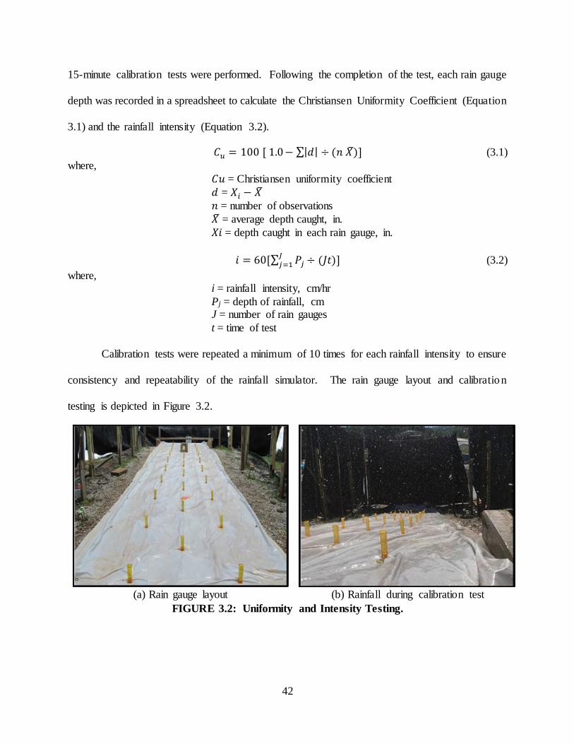
42
15-minute calibration tests were performed. Following the completion of the test, each rain gauge
depth was recorded in a spreadsheet to calculate the Christiansen Uniformity Coefficient (Equation
3.1) and the rainfall intensity (Equation 3.2).
𝐶𝑢 = 100 [ 1.0 − ∑|𝑑| ÷ (𝑛 𝑋)] (3.1)
where,
𝐶𝑢 = Christiansen uniformity coefficient
𝑑 = 𝑋𝑖 − 𝑋
𝑛 = number of observations
𝑋 = average depth caught, in.
𝑋𝑖 = depth caught in each rain gauge, in.
𝑖 = 60[∑ 𝑃𝑗 ÷ (𝐽𝑡)𝐽𝑗=1 ] (3.2)
where, i = rainfall intensity, cm/hr
Pj = depth of rainfall, cm J = number of rain gauges
t = time of test
Calibration tests were repeated a minimum of 10 times for each rainfall intensity to ensure
consistency and repeatability of the rainfall simulator. The rain gauge layout and calibration
testing is depicted in Figure 3.2.
(a) Rain gauge layout (b) Rainfall during calibration test
FIGURE 3.2: Uniformity and Intensity Testing.

43
3.2.1 Drop Size Distribution
After the desired uniformity and rainfall intensity was reached, the flour pan test was used
to evaluate the drop size distribution for the 2, 4, and 6 in. per hr (51, 102, and 152 mm per hr)
rainfall intensities (Laws and Parsons 1943). An 8.5 in. (216 mm) diameter aluminum pie pan was
filled to the edge with sifted Pillsbury all-purpose flour. The excess flour was struck off with a
straight edge to create a smooth surface along the edge of the pie pan. The rainfall simulator was
turned on to the desired rainfall intensity and the covered flour pan was placed on a level wooden
stand. The top of the aluminum pie pan was removed by pulling the cover toward the experimenter
for 2 to 4 seconds before recovering the pan. This procedure was performed at the top, middle,
and bottom of the slope for each rainfall intensity. The flour pan sampling procedure is depicted
in Figure 3.3.
(a) Covered flour pan (b) Uncovered flour pan
FIGURE 3.3: Flour Pan Field Procedure.
The flour was air dried for a minimum of 12 hours. The air-dried flour was gently sieved
through a No. 70-wire mesh sieve. The pellets were inspected to remove combined or misshapen
pellets and the remaining flour pellets were placed in the oven for 2 hours at 230˚F (110˚C). The
oven dried pellets were sieved through the No. 4, 8, 10, 14, 20, and 30 sieves. The flour pellets

44
retained on each sieve were counted and weighed. The analysis of the flour pellets is depicted in
Figure 3.4.
(a) Flour pan (b) No. 70 sieve pellets
(c) Testing sieves (d) Weighing pellet samples
FIGURE 3.4: Flour Pan Lab Testing.
Each rainfall intensity collected three flour pan samples, which were all added together for
drop size distribution analysis. The total weight of the flour pellets retained on each sieve was
calculated by adding the weights for all three samples. The average weight of the pellets retained
on each sieve is determined by dividing the total weight per sieve by the total number of pellets.
The mass ratio was calculated to convert the mass of the average pellet into the mass of the average
drop using Equation 3.3.

45
𝑀𝑅 = (0.038) ∗ ln(𝑊𝑎𝑣𝑔 ) + 1 (3.3)
where, MR = mass ratio
Wavg = average pellet weight, mg
The average diameter of the pellets was calculated by multiplying the average weight and
the mass ratio as depicted in Equation 3.4.
𝐷𝑎𝑣𝑔 = √6
𝜋× 𝑊𝑎𝑣𝑔 × 𝑀𝑅
3 (3.4)
where,
Davg = average drop diameter, mm Wavg = average weight, mg
MR = mass ratio
The adjusted pellet weight was calculated by multiplying the total pellet weight for each
sieve by the sieves corresponding mass ratio. The adjusted mass percentage was calculated by
dividing the adjusted total pellet weight per sieve by the total adjusted pellet weight for pellets
retained on all the sieves. The fall velocity was calculated by developing a regression equation
from the raindrop fall velocity measurements from 15 ft (4.7 m). The regression equation was
formed by plotting the raindrop size and the corresponding fall velocity from Figure 3.5. The
regression equation is depicted by Equation 3.5.
FIGURE 3.5: Raindrop Fall Velocity Chart (ASTM 2015).

46
𝑦 = −0.1667𝑥 2 + 1.8235𝑥 + 2.8602 (3.5) where,
y = fall velocity, m/s
x = raindrop size, mm
The total rainfall volume for each rainfall intensity was calculated by converting the rainfa ll
intensity to feet and multiplying by the test plot area of 320 ft2 (29.7 m2). The rainfall weight was
calculated by multiplying the rainfall volume by 62.4 lb. per ft3 (1000 kg per m3), the density of
water. The total rainfall weight was converted to slugs by dividing the weight by 32.2 ft per s2
(2.97 m2 per s). The incremental weight of rainfall retained on each sieve was calculated by
multiplying the rainfall mass by the percentage of rainfall. The kinetic energy for each sieve was
calculated by implementing Equation 3.6.
𝐾𝐸 = 1
2𝑚𝑣2 (3.6)
where,
KE = kinetic energy of sieve, m = incremental rainfall mass, slug
v = raindrop fall velocity, ft/s
The kinetic energy was then converted to foot-tons by dividing the original kinetic energy
by 2000 lb. per ton (0.5 kg per metric ton). The total kinetic energy for the test plot is calculated
by dividing the KE in foot-tons by the area of the test plot in acres as depicted by Equation 3.7.
𝐸 = 𝐾𝐸
(𝐴
43560) (3.7)
where,
E = total kinetic energy A = total test plot area, ft2
KE = kinetic energy, ft-ton
The total kinetic energy for each sieve was summed together for all three-rainfa l l
intensities. The maximum 30-minute rainfall intensity was calculated by determining the
maximum possible rainfall intensity occurring during the hour-long experiment. Therefore, I30
was calculated using Equation 3.8.

47
𝐼30 = (4
𝑖𝑛
ℎ𝑟×10 min)+(6
𝑖𝑛
ℎ𝑟×20 min)
30 𝑚𝑖𝑛 (3.8)
where,
I30 = maximum 30-minute rainfall intensity, in.
The theoretical erosivity index was calculated by multiplying the total kinetic energy with
a conversion of 0.01 and I30. The theoretical erosivity index was later used to aid in the Revised
Universal Soil Loss Equation (RUSLE) calculations analyzing product performance.
3.3 VALIDATION PROCEDURES
Following the completion of calibration testing for the 2, 4, and 6 in. per hr (51, 102, and
152 mm per hr) rainfall intensities, bare soil control tests were performed to provide a benchmark
comparison to erosion control product performance.
3.3.1 Slope Preparation
Prior to rainfall simulation testing, the test slope must be prepared in a consistent and
repeatable manner. To remove rills or slope damage from prior testing, the entire test slope was
tilled to a minimum depth of 4 in. (10.2 cm). The tilling process is depicted in Figure 3.6.
(a) Tilling test slope (b) Till bottom of test slope
FIGURE 3.6: Tilling Test Slope.
After the slope was tilled, the soil was raked to remove any clumps and to create a level
soil depth across the slope. Dry screened soil was raked into the test plot until the optimal soil

48
elevation was reached across the entire test plot. If the soil was too dry, water was added until the
moisture content was within 5% of the optimal moisture content. A 24 by 48 in. (0.61 by 1.22 m)
turf roller was placed at the bottom of the test slope against one edge of the plot. The turf roller
was rolled up and down the slope with a mounted electronic winch three times. Then the turf roller
was moved to the other half of the test plot and the same number of passes was performed. Lastly,
the turf roller was moved to the center of the plot where one pass is performed to remove any
inconsistencies from prior compacting. The desired compaction rate for the loam and sandy loam
soils is 86±6%. The compaction process is depicted in Figure 3.7.
(a) First half compacted (b) Second half compacted
FIGURE 3.7: Slope Compaction.
3.3.2 Drive Cylinder Compaction
Once the slope is compacted, the compaction and moisture content are evaluated through
the Standard Test Method for Density of Soil in Place by the Drive-Cylinder Method (ASTM
D2937). Three numbers between 1 and 60 were selected by a random number generator to
determine the drive cylinder test locations depicted in Figure 3.8.

49
FIGURE 3.8: Drive Cylinder Test Locations (Horne et al. 2017).
The drive cylinder was driven into the slope. The cylinder was removed by digging around
the front edge and picking the sample and cylinder up with a flat tool. Excess soil was removed
from the bottom and cylinder edge. The approximate thickness of the soil sample was measured
with a caliper. The wet soil sample was weighed before the moisture content and percent
compaction were determined. The drive cylinder compaction test procedure is depicted in Figure
3.9.

50
(a) Aligning cylinder with the slope (b) Dropping the weight
(c) Leveled bottom (d) Weighing sample
FIGURE 3.9: Drive Cylinder Compaction Procedure.
Immediately following the drive cylinder compaction test, the moisture content of the soil
sample was determined by following the Determination of Water Content of Soil by Microwave
Oven Heating (ASTM D4643). The drive cylinder soil sample was placed in a microwave safe
dish, which was weighed and then heated in the microwave for three minutes. The sample was
removed, weighed, and placed back in the microwave for one additional minute. This process was
repeated until the change in mass was 0.1% of the initial wet mass or there is no change in mass.
The final dry mass was used to calculate the moisture content in Equation 3.6.

51
𝑤 = (𝑀1−𝑀2
𝑀2− 𝑀𝑐) × 100 (3.6)
where, w = water content, % M1 = mass container and wet soil, g
M2 = mass container and dry soil, g
Mc = mass container, g
The allowable moisture content must be within 5% of the optimal moisture content. The
wet density of the soil sample was calculated using Equation 3.7.
𝜌𝑤𝑒𝑡 = (𝑀1−𝑀2)
𝑉 (3.7)
where,
ρwet = wet density, g/cm3 M1 = mass cylinder and wet soil sample, g
M2 = mass cylinder, g
V = volume of cylinder, cm3
The in-place dry density was then calculated using the wet density of the soil shown in
Equation 3.8.
𝜌𝑑 = 𝜌𝑤𝑒𝑡
(1+(𝑤
100))
(3.8)
where,
ρd = dry density, g/cm3
ρwet = wet density, g/cm^3
w = water content, %
The dry unit weight was then calculated using the in-place dry density in Equation 3.9.
𝛾𝑑 = 62.4 × 𝜌𝑑 (3.9) where,
𝛾𝑑 = dry unit weight, lb/ft3
ρd = dry density, g/cm3
The dry unit weight for each drive cylinder sample was divided by the maximum dry unit
weight of the soil to determine the percent compaction. The ASTM D6459-19 does not specify a
compaction rate for the test plot soil. Therefore, a compaction rate of 86±6% was selected for
rainfall simulation testing. This compaction rate does not meet the typical 90 to 95% compaction
rate for fill slopes, but since these slopes are typically dressed with top soil, which is only tracked

52
in, this compaction amount will be more reflective of field conditions. If the percent compaction
was not within 86±6 % limits, then additional slope preparation must be performed. This process
was repeated until the water content and compaction meet the desired values.
3.3.3 Turbidity
Water samples were collected at the bottom of the test plot where all runoff was funne led
to a single location where a 7 fl oz. (200 mL) sampling bottle catches the water sample. The
collection of water samples started once the runoff began and continued at a three minute
increment until runoff stops. Following the completion of the rainfall simulation and the collection
of water samples, the samples were transferred to the lab for testing. First, the turbidimeter was
recalibrated using standard samples. Then each water sample bottle was shaken to thoroughly mix
all sediment in the solution. The water sample was transferred to a 33.8 fl oz. (1,000 mL) beaker
and placed on a magnetic stirrer. The sample was continuously mixed throughout the entire testing
process. A pipette was used to fill the turbidity sample cell to the line with 0.51 fl oz. (15 mL) of
sample. The cell was placed in the turbidimeter and the reading was recorded. The preparation
and testing of the turbidity measurements is depicted in Figure 3.10.
(a) Turbidimeter (b) Turbidity sample
FIGURE 3.10: Turbidity Lab Testing.

53
If the water sample over ranges, the original sample was diluted 1:2 by mixing 3.4 fl oz.
(100 mL) of deionized water in a beaker with 1.70 fl oz. (50 mL) of sample. The cell was filled
with the diluted sample and the measurement recorded. The dilution process was repeated until
the turbidimeter recorded a measurement.
3.3.4 Total Suspended Solids
Following the completion of the turbidity testing, the same diluted sample was used to
determine the TSS for each water sample. Before testing began, the glass microfiber filter
membranes were pre-washed with 0.34 fl oz. (10 mL) of deionized water. The filter membranes
were placed in numbered aluminum crinkle dishes and placed in the oven at 117˚F (103˚C) for one
hour. The crinkle dishes were removed from the oven and placed in a desiccator to cool to room
temperature. Once at room temperature, the crinkle dish and filter membrane were weighed on
the analytical balance and recorded to the nearest 0.0001 grams. Tweezers were used to move the
filter membrane from the crinkle dish to the filtering apparatus. A pipette transferred 0.85 fl oz.
(25 mL) of diluted solution to the filter. The filtering machine was turned on to suction the water
through the filter. The filtrate on the filter was rinsed with three 0.34 fl oz. (10 mL) portions of
deionized water. The filter membrane was removed from the apparatus with tweezers, placed in
the assigned crinkle dish, and placed in the oven at 103˚C for one hour. Once the filter membranes
were dry and have cooled to room temperature, each filter membrane and crinkle dish were
weighed to the nearest 0.0001 grams. The procedure used to determine the TSS for water samples
is depicted in Figure 3.11.

54
(a) Rinsing filters (b) Mixing water samples
(c) Filtered sample (d) Drying samples
FIGURE 3.11: TSS Lab Testing.
3.4 PRODUCT APPLICATION
All tested product installation followed the standards in the Alabama Handbook for Erosion
Control, Sediment Control and Stormwater Management on Construction Sites and Urban Areas
and the ALDOT Standard Specifications for Highway Construction. Product manufacture r’s
recommendations were also followed when necessary.
3.4.1 Loose Straw
Once the slope preparation procedure has been completed, loose dry wheat straw was
applied to the slope for the blown, crimped, and tackifier straw tests. An application rate of 2 tons
per acre (4483 kg per ha) was installed by hand as designated by the Alabama Handbook for

55
seeding applications and ALDOT. The test plot and straw was divided into four even sections and
spread by hand across the test plot to ensure a consistent application rate. The loose straw
application is depicted in Figure 3.12.
(a) Straw application (b) Finished application
FIGURE 3.12: Loose Straw Application.
3.4.2 Loose Straw with Tackifier
Once the slope preparation and loose straw application procedures were completed, a
tackifier was sprayed on the straw. The tackifier was installed at an application rate of 50 lb. per
acre (56 kg per ha). Four metal buckets were filled with 8 gallons (30.3 L) of water and one fourth
of the tackifier to be installed. The tackifier was mixed with a drill mixer until the powder
dissolved into a thick blue solution. Four gallons of tackifier solution was poured into a backpack
sprayer and spread across one eighth of the test plot (40 ft2). Manufacturer recommendations were
followed for the curing time of the tackifier solution before rainfall simulation testing was
performed. The powder and mixed Tacking Agent 3 are depicted in Figure 3.13.

56
(a) Power form Tacking Agent 3 (b) Mixed tackifier
FIGURE 3.13: Tackifier Application.
3.4.3 Crimped Straw
Once the slope preparation and loose straw application procedures were completed, the
straw was crimped using the following procedure. A crimper was constructed using two notched
flat coulter blades and wheelbarrow handles. Each blade was spaced eight inches (20.3 cm) apart
as specified by Section 656 in the ALDOT Standard Specifications for Highway Construction.
The crimper was rolled across the straw covered slope perpendicular to the flow direction. The
straw was imbedded a minimum of two inches (5.1 cm) into the soil. The crimping procedure is
depicted in Figure 3.14.
(a) Crimping perpendicular to slope (b) Crimped straw
FIGURE 3.14: Crimping Straw.

57
3.4.4 Hydraulic Erosion Control Products
A 300-gallon (1,135 L) Turf Maker hydroseeder was used for the mixing and application
of the hydraulic erosion control products (HECP). Prior to rainfall simulation testing, the
hydroseeder was calibrated. Eight four-foot by two-foot (1.21 m by 0.3 m) plywood sheets were
placed on a 3H:1V slope. The hydroseeder sprayed the hydraulic mulch onto the plywood sheets
by moving the nozzle side to side. Following each pass of the hydraulic mulch nozzle, one sheet
of plywood was removed. Once the installation for all eight sheets of plywood were complete, the
hydraulic mulch was allowed to dry. The dry product was scrapped from the boards and weighed
to the nearest gram. The weight of mulch on each plywood sheet was converted to pounds per
acre to determine the optimal number of sprays per application rate. The hydroseeder used for
testing is depicted in Figure 3.15.
FIGURE 3.15: Hydroseeder used for Hydromulch Testing.
To prevent clogging in the hydroseeder, the hydraulic mulch was hand shredded prior to
mixing. One 50 lb. (22.7 kg) bale of hydraulic mulch was used for each experiment. Following a
water to mulch ratio of 2:1, 100 gallons (379 L) of water was needed to mix with 50 lb. (22.7 kg)
of mulch. Prior to mixing the product, an extra 50 gallons (189 L) of water was added to the tank
and pumped out to prime the pump and flush the system. With the remaining 100 gallons (379 L)

58
of water in the tank, the agitator was turned on and the product was slowly added to the tank. The
hydraulic mulch was allowed to mix for 20 minutes before installation began.
Once the hydraulic mulch had mixed for 20 minutes, the product can be installed. Plywood
sheets were placed along one edge of the test plot to monitor the product application rate. The
pump was turned on and all excess water was removed from the pump and hose until the product
was flowing at a steady rate. The product was first installed from the bottom of the test plot by
spraying the hydraulic mulch side to side. Then the hydraulic mulch was sprayed from the top of
the slope to ensure consistent coverage. The hydraulic mulch was allowed to cure for a minimum
of 24 hours before being tested. Once the hydraulic mulch on the plywood boards was dry, the
application rate was checked by weighing the product to the nearest gram and converting to pounds
per acre. Target application rates for products were installed as designated by the manufacturer.
The hydraulic mulch installation is depicted in Figure 3.16.
(a) Bottom install (b) Top install
FIGURE 3.16: Hydraulic Mulch Application.
3.4.5 Rolled Erosion Control Products
Temporary erosion control blankets (ECBs) were installed on the test plot using the
following installation procedure. Based on the ALDOT Standard section 659, type S3 blankets
were evaluated for the 3H:1V slope. The test slope must first be prepared resulting in a smooth

59
and level slope. Once the slope preparation procedure was complete, a 6 in. by 6 in. (15.2 cm by
15.2 cm) trench was created along the top of the test plot. The ECB was anchored into the trench
following the manufacturer guidelines. The product was rolled down the slope without stretching
or pulling the blanket. The product manufacturers slope anchoring guidelines were followed for
an 8-foot (2.43 m) wide blanket. Once the product reached the bottom of the test plot, it was cut
so that the blanket was flush with the bottom of the test plot. The ECB installation process is
depicted in Figure 3.17.
(a) 6” by 6” trench (b) Trenched ECB
(c) Installing ECB (d) Installed ECB
FIGURE 3.17: Erosion Control Blanket Installation.

60
3.5 RAINFALL SIMULATION TEST PROCEDURE
Throughout the duration of this project, two different test procedures have been used. The
first test procedure was used on a sandy loam soil. After testing on the sandy loam soil, the studies
interpretation of ASTM D6459 was changed. The soil type and test procedure initially used were
not meeting the standard as well as not providing the data for product C-factor calculations. The
soil type was changed to a loam soil and a new test procedure used for testing. Prior to testing for
both procedures, the compaction and moisture content of the slope met the designated limits. Once
the slope was properly prepared, six rain gauges were installed on the slope at 10, 20, and 30 ft (3,
6, and 9 m) and from the top of the slope in 2 columns.
3.5.1 Sandy Loam Test Procedure
The sandy loam test procedure consisted of a 60 minute test duration with three sequentia l
20 minute rainfall intensities of 2, 4, and 6 in. per hr (51, 102, and 152 mm per hr). At the
beginning of testing, the pump was turned on to build up pressure in the rainfall simulator. Once
the desired pressure was reached, the first switch was turned on to initiate the 2 in. per hr (51 mm
per hr) rainfall intensity. Once runoff beings entering the catch basin, waters samples were
collected at 3-minute increments until runoff stops following the experiment. Just before the 20
minute point of the test, photos were taken of the test plot conditions. Once the test duration
reaches 20 minutes, turn on an additional switch to initiate the 4 in. per hr (102 mm per hr) rainfa ll
intensity. Just before the 40 minute point in the test, photos were taken of the test plot conditions.
Then, the third switch was turned on to produce the 6 in. per hr (152 mm per hr) rainfall intens ity.
After 60 minutes of testing, the pump and rainfall simulator were turned on. Immedia te ly
following the test, the total rainfall depth collected during the experiment was recorded and the

61
slope conditions were photographed. The discharge over time that entered the catch basin was
measured with a water depth logger, which was placed in the catch basin.
3.5.2 Loam Test Procedure
Each test had a duration of 60 minutes and was divided into three sequential 20 minute
sections with 2, 4, and 6 in. per hr (51, 102, and 152 mm per hr) rainfall intensities. The rainfa ll
intensity was adjusted by using three switches that each control ten sprinklers. The test was
momentarily paused at the 20 and 40 minute mark. During the pause, the rain gauge measurements
were recorded, the soil collection container was changed, and the slope was photographed. Once
these tasks were completed, the test was continued. Water samples were collected every three
minutes. If no discharge off the slope was occurring, then no runoff sample would be collected.
Runoff was collected at three-minute intervals with time being measured once rainfall is initiated.
These water samples were later evaluated for TSS and turbidity measurements using the previously
discussed analysis procedures. The discharge over time of the test plot was determined by
recording the time it takes the runoff to fill a known volume. The same known volume could not
be used for each storm event due to the significant differences in runoff. Therefore, a smaller
volume is used for the 2 in. per hr storm event and a larger known volume for the 4 and 6 in. per
hr (102 and 152 mm per hr) events. The discharge measurements were recorded every two minutes
for the full duration of the test. The sample collection process is depicted in Figure 3.18.

62
(a) Water sample collection (b) Discharge measurement
FIGURE 3.18: Water Runoff Analysis.
The runoff caused by each rainfall intensity was separated into separate containers. The 2
and 4 in. per hr (51 and 102 mm per hr) rainfall intensity runoffs were diverted into independent
galvanized metal tanks. The 6 in. per hr (152 mm per hr) rainfall intensity runoff was collected in
the catch basin located at the bottom of the test slope. The sediment was allowed to settle for a
minimum of 24 hours before the excess water was removed from the surface. The total dry mass
of sediment for each rainfall intensity was determined by weighing all of the wet sediment and
collecting representative samples to determine the moisture content of the soil. The runoff
collection and dry sediment determination processes are depicted in Figure 3.19.

63
(a) Galvanized tanks (b) Catch basin
(c) Weighing soil (d) Moisture sample
FIGURE 3.19: Soil Loss Analysis.
3.6 SOIL ANALYSIS
Before rainfall simulation testing and the GAI accreditation was pursued, a soil
classification must be determined for the United States Department of Agriculture (USDA)
classification system and Unified Soil Classification System (USCS). The soil stockpile on site
was analyzed through a sieve analysis, proctor compaction, Atterberg limits, and a hydrometer
test. Several soils were evaluated to determine the soil that best fit ASTM D6459 requirements.

64
3.6.1 Dry Sieve Analysis – ASTM C136
A dry sieve analysis was performed following ASTM C136. A 0.66 lb. (300-g) soil sample
was weighed and dried to constant mass at a temperature of 110±5˚C (230±10˚F). Sieves No. 4,
10, 20, 40, 60, 100, 200, and pan were selected for the analysis. Before the soil was placed in
sieves, each sieve and the pan was weighed. The entire sample was placed on the No. 4 sieve and
covered by the lid. The stack of sieves was placed in a mechanical sieve shaker, which was run
for 5 minutes. Once the shaking process was completed, the sieve stack was removed from the
mechanical shaker. Each sieve was individually weighed with the retained soil. The percent
passing and percent retained on each sieve was calculated to obtain the particle size distribution.
The sieve analysis process is depicted in Figure 3.20.

65
(a) Weighed soil sample (b) Soil placed in sieve
(c) Sieve shaker (d) Post sieve machine
FIGURE 3.20: Dry Sieve Analysis.
3.6.2 Wet Sieve Analysis – ASTM C117
A wet sieve analysis was performed on the proposed testing soil because the finer soil
particles were clumping together with larger soil particles resulting in an inaccurate particle size
distribution. Before the soil analysis was started, the soil was dried at 230˚F (110˚C) until a
constant mass was reached. A soil sample of 0.22 lb. (100 g) was weighed and placed in a
container. Water was added to the soil sample and thoroughly mixed to separate the soil particles.
The water containing the suspended and dissolved solids was poured over the No. 16 and 200
sieve. Another charge of water was added to the bowl and mixed to separate any additiona l
particles. The mixed water was poured through the sieves. This process was repeated until the

66
water was clear. The material washed through the sieve was dried on a hot plate and in the oven.
The soil not passing the No. 16 and 200 sieve was dried in the oven. Once the retained soil was
dried, the soil was evaluated following the procedure for a dry sieve analysis. The soil passing the
No. 200 sieve was weighed and used for hydrometer testing. The wet sieve analysis procedure is
depicted in Figure 3.21.
(a) Wetting soil (b) Pouring water through sieves
FIGURE 3.21: Wet Sieve Analysis Testing.
3.6.3 Proctor Compaction Test – ASTM D698
The optimal moisture content and the maximum dry unit weight of the soil sample was
determined through the Standard Test Methods for Laboratory Compaction Characteristics of Soil
Using Standard Effort (ASTM D698). The moist soil sample was sieved through the No. 4 sieve
before being used in the experiment. A minimum of five test sub-specimens were created to
generate a compaction curve. A sub-specimen of 5.51 lb. (2,500 g) was placed in a large metal
bowl and water was mixed into the soil sample. Before placing the soil into the mold, the proctor
mold was weighed without the extension collar. The soil was installed in three separate lifts to the
mold and compacted with 25 blows following the pattern in Figure 3.22.

67
FIGURE 3.22: Proctor Compaction Pattern (ASTM 2012).
Once the compaction was completed, the extension collar was removed and a flat edge was
used to remove all excess soil. The mold and soil were weighed before the soil cylinder was
removed from the mold. Representative soil samples were collected from different areas of the
compacted soil cylinder, weighed, and placed in the oven at a temperature of 140˚F (60˚C). This
process was repeated by incrementally increasing the amount of water added to a new 5.51 lb.
(2,500 g) soil sample. Once the dry weights of the representative samples were measured, a
compaction curve was created to determine the optimal moisture content and maximum dry unit
weight of the soil stockpile. The proctor compaction procedure is depicted in Figure 3.23.

68
(a) Adding water to soil (b) Compacting soil into cylinder
(c) Leveling top of cylinder (d) Leveled cylinder
FIGURE 3.23: Proctor Compaction Procedure.
3.6.4 Atterberg Test – ASTM D4318
The procedures in ASTM D4318 were followed to determine the liquid limit, plastic limit
and the plasticity index of each soil sample. Before the sample was sieved through the No. 40
sieve, the soil was dried and removed any clumps. All material passing the No. 40 sieve was used
for the liquid limit and plastic limit test.
3.6.4.1 Liquid Limit
A sample of the soil passing the No. 40 sieve was placed in a mixing bowl and water was
added from a spray bottle. The target moisture content for the first trial will result in 25 to 35

69
drops. Once the desired moisture content was reached, the soil was spread with a spatula into the
cup with a depth of 0.39 in. (10 mm). The soil was evened out and moved around to ensure no air
bubbles were in the soil. A groove was formed down the center of the cup to divide the soil in
half. The drop cup was lifted by turning the handle at a rate of 2 drops per second until the two
halves come in contact. The number of drops required for the two halves to touch was recorded.
A moisture sample was then selected and weighed before placed in the oven. The liquid limit
procedure is depicted in Figure 3.24.
(a) Mixing sieved soil (b) Cup installation
FIGURE 3.24: Liquid Limit Testing.
Once the 25 to 35 drop target sample was reached, two additional samples with a 20 to 30
and 15 to 25 drops target was pursued. Water was added to the previous soil sample to achieve
the lower drop ranges. The sample dropping and measuring process was repeated for these two
samples.
3.6.4.2 Plastic Limit
A 0.71 oz. (20 g) sample of the soil prepared by the liquid limit test from the second mixing
was used to determine the plastic limit of the soil. A 0.05 to 0.07 oz. (1.5 to 2 g) portion of the
sample was selected and formed into an ellipsoidal mass. The soil mass was rolled between the
palms of the experimenters hands and on the glass plate until a uniform diameter of 0.13 in. (3.2

70
mm) is reached. The sample was then reformed into an ellipsoid and rolled again. The soil was
continually rolled and reformed until the sample crumbles. The crumbled soil was placed in a dish
and the process was repeated until 0.21 ounces (6 g) of soil was obtained. This entire process was
repeated to result in having two 0.21 ounces (6 g) samples to dry in the oven. The plastic limit test
is depicted in Figure 3.25.
(a) Rolling wet soil (b) Rolled soil sample
FIGURE 3.25: Plastic Limit Testing.
3.6.5 Hydrometer Analysis – ASTM D7928
Prior to the performance of a hydrometer test, a wet sieve analysis was performed to soil
particles passing the No. 200 sieve. A 1.76 ounce (50 g) sample of the soil passing the No. 200
sieve was weighed out and placed into a dispersion (or malt mixer) cup. Then, 3.38 fluid oz. (100
mL) of sodium metaphosphate was measured in a graduated cylinder and placed in the dispersion
cup with the soil sample. Water was used to wash all soil to the bottom of the cup. The dispersion
cup was placed on the mixer and run for 5 minutes. The solution was transferred from the
dispersion cup to the sedimentation cylinder. The dispersion cup was rinsed with a plastic squeeze
bottle and added to the sedimentation cylinder. The sedimentation cylinder was filled with distilled
water to 33.81 fluid ounces (1,000 mL). The preparation of the soil solution is depicted in Figure
3.26.

71
(a) Soil sample passing No. 200 sieve (b) Malt mixer
(c) Turning sedimentation cylinder (d) Hydrometer reading
FIGURE 3.26: Hydrometer Analysis Procedure.
A control cylinder was filled with 33.81 fluid oz. (1000 mL) of water used to calibrate the
hydrometer (152H model). Before the hydrometer test time started, a rubber stopper was placed
over the sedimentation cylinder to agitate for 1 minute by turning the cylinder upside down and
back 60 times. Immediately following the agitation, the stopper was removed and the hydrometer
was placed in the soil solution. A stopwatch was started when the hydrometer was placed in the
sedimentation cylinder. Hydrometer readings were taken at 0.25, 0.5, 1, and 2 minutes. The
hydrometer was removed from the sedimentation cylinder and placed in the control cylinder.
Thirty seconds before the next reading, the hydrometer was placed back in the sedimentat ion

72
cylinder. Measurements were recorded at 4, 8, 15, 30, and 60 minutes and 2, 4, 6, 8, 24, and 48
hours. After each measurement was recorded, the hydrometer was removed from the
sedimentation cylinder and placed in the control cylinder. The sedimentation cylinder was covered
with the stopper between measurements to prevent evaporation. The water temperature was
measured during each measurement with a thermometer. The temperature correction factor was
determined through the use of Equation 3.10.
𝐹𝑡 = −4.85 + 0.25𝑇 (3.10) where, Ft = temperature correction
T = measure temperature, ˚C
Once the test was complete, the corrected hydrometer reading was calculated using
Equation 3.11. The percent finer for the hydrometer readings was determined using Equation 3.12.
𝑅𝑐𝑝 = 𝑅 + 𝐹𝑡 + 𝐹𝑧 (3.11)
where,
Rcp = corrected hydrometer reading R = hydrometer reading
Ft = temperature correction
Fz = hydrometer zero correction
% 𝐹𝑖𝑛𝑒𝑟 =(𝐴×𝑅𝑐𝑝×100 )
𝑊𝑠 (3.12)
where, A = correction for specific gravity
Ws = Dry weight of soil used for hydrometer analysis
Rcp = corrected hydrometer reading for percent finer
3.7 REVISED UNIVERSAL SOIL LOSS EQUATION (RUSLE)
The Revised Universal Soil Loss Equation (RUSLE) was used to calculate the soil
erodibility factor (K) of the tested soil and the cover management factor (C-factor) of erosion
control practices. The drop size distribution data and calculations in section 3.2.1 are used along
with the soil loss and rain gauge measurements for each rainfall intensity. The bare soil control
test was used to calculate the K-factor for the three corresponding erosion control product tests.

73
3.7.1 Soil Erodibility Factor – K-Factor
The K-Factor was calculated using the rain gauge measurements and soil loss (lb.) for each
20 minute rainfall intensity segment of the bare soil control test. The rain gauge measurements
were used to calculate the average rainfall in inches and the maximum 30-minute rainfall intens ity
(I30). The total soil loss for each rainfall intensity was inserted and converted from pounds to tons.
The average soil loss (A) in tons/acre was calculated for each intensity by dividing the soil loss
(tons) by the acreage of the rainfall simulator test plot.
Following these calculations, a graph is created plotting the incremental R-factor vs. the
incremental A (tons/acre). From the three points plotted on the graph, a linear trendline is used to
determine the trendline equation. The slope of the trendline equation is equal to A/R. The
theoretical R-factor is used in the trendline equation to calculate the average A (tons/acre) from the
entire experiment. The RUSLE equation is reformatted to solve for the K-factor as depicted in
Equation 3.13.
𝐾 = 𝐴
𝑅×𝐿𝑆×𝐶×𝑃 (3.13)
where, K = soil erodibility factor A = average soil loss (ton/acre)
R =rainfall erosivity factor LS =length slope steepness factor
C = cover management factor
P = support practice factor
Since a bare soil control test was being evaluated, the C-factor and P-factor are 1.0. The
LS value is the calculated value for the length and steepness of the test plot. Once all of the
equation values are determined, the K-factor was calculated. This K-factor will be used for the
three product tests it was paired with. A bare soil control test was performed for every three
product experiments.

74
3.7.2 Cover Management Factor – C-Factor
The C-factor for a product was calculated by inserting the incremental rain gauge
measurements and the incremental soil loss data into the drop size distribution data from section
3.2.1. This will calculate the incremental EI30 value (R). The incremental average soil loss (A)
was calculated by dividing the soil loss in tons by the acreage of the test plot. Once these values
were calculated, a graph was created to plot the R-factor vs. A (ton/acre). The three data points on
this graph are used to create a linear trendline equation. The slope of the linear trendline equation
equals A/R. The average A (tons/acre) for the experiment was calculated by solving the trendline
equation with the theoretical R-value. The RUSLE equation was arranged to solve for the C-factor.
The C-factor for the product was calculated using the slope of the trendline A/R and a P-factor of
1.0.
Once three experiments of the same product have been completed, the average C-factor for
the product must be determined. Two separate methods were used to calculate the C-factor for
each erosion control product. The first method plotted the incremental C-factor versus the
incremental R-factor for all three of the products experiments. The 2 inch per hour (52 mm per
hr) rainfall intensity data was not included because the C-factor was near zero resulting in a skewed
trendline equation. A linear trendline equation was fit to the 4 and 6 inch per hour (102 and 152
mm per hr) data points. The resulting trendline equation was used to calculate the C-factor of the
product by solving for the theoretical R-factor of 182.02.
The second method used to solve for the product C-factor plotted the incremental soil loss
(A) tons/acre versus the incremental R-factor for each individual experiment. A trendline equation
was determined for each of the graphs and used to calculate the A in tons/acre for each test that

75
correlates with the theoretical R-factor of 182.02. The resulting A-factor was averaged for all of
the experiments and used in the RUSLE equation.
3.8 SUMMARY
This chapter summarizes the procedures used for the calibration testing, validation testing,
erosion control practice installation, rainfall simulator testing procedure and the soil analysis.
These procedures were used to meet the requirements of ASTM D6459-19 to evaluate erosion
control practices on the AU-ESCTF rainfall simulator. These procedures were used to obtain the
results summarized in Chapter 4.

76
CHAPTER 4: RESULTS AND DISCUSSION
4 CHAPTER 4: RESULTS AND DISCUSSION
4.1 INTRODUCTION
Calibration testing was performed on the AU-ESCTF rainfall simulator to verify that the
simulator could produce consistent rainfall that followed the ASTM D6459 standards for intens ity,
uniformity, and drop size distribution. Once the calibration testing was completed, a soil analysis
was performed on the soil stockpiles to verify that the soil was classified as a clay, loam, or sand.
Once all of the preliminary testing was performed, bare soil and erosion control practices were
analyzed through full-scale rainfall simulation testing. This chapter will present the experimenta l
results and a statistical analysis of these results.
4.2 CALIBRATION RESULTS
The procedures described in Section 3.2 produced rainfall data, which reflects the
performance of the rainfall simulator. The raw calibration data for each experiment is provided in
Appendix C. The data recorded from calibration testing was used to calculate the experimenta l
rainfall intensity, uniformity, and drop size distribution for each target rainfall intensity of 2, 4,
and 6 in. per hour (51, 102, and 152 mm per hr).
4.2.1 Uniformity and Intensity
The initial rainfall simulator consisted of six risers each with four sprinklers designed to
produce a 2-year, 24-hour storm event for Alabama. During the calibration process, the rainfa ll
simulator was redesigned to have eight riser each with three sprinklers to product the 2, 4, and 6
in. per hour (51, 102, and 152 mm per hour) rainfall intensities. Calibration testing determined
that the top and bottom of the test plot was not receiving the same rainfall coverage as the rest of

77
the test plot. Therefore, two additional risers were placed at the uphill and downhill sides of the
test plot. Following the placement of two additional rainfall risers, calibration tests were
performed to verify that the riser placement was producing uniform rainfall throughout the test
plot. Once the riser placement was finalized, a total of 30, 15 minute calibration tests were
performed with 20 rain gauges installed on the test plot. A minimum of ten calibration tests were
performed for each rainfall intensity. If the standard deviation between the ten tests was less than
0.1 in. per hr (0.25 cm per hr), no additional calibration testing was required. Each rainfall intens ity
in this experiment had a standard deviation less than 0.1 in. per hr (0.25 cm per hr) and therefore
only required ten tests. During the calibration process, 6 psi (41 kPa) and 10 psi (69 kPa) pressure
regulators were installed to determine which pressure resulted in the best rainfall conditions. The
6 psi (41 kPa) pressure regulator was selected for testing because it generated larger drop sizes as
well as a higher rainfall uniformity. The calibration summary results are depicted in Table 4.1.
TABLE 4.1: Rainfall Intensity Results
Theoretical Rainfall Intensity 2 in. per hr 4 in. per hr 6 in. per hr
Experimental Intensity (in/hr) 2.08 4.12 6.07
Rainfall Intensity Percent Error (%) 4.00 3.00 1.17
Standard Deviation 0.04 0.06 0.07
Number of Tests 10 10 10
Note: 1 inch per hour = 25.4 millimeter per hour
The experimental rainfall intensity for each calibration test was averaged and compared to
the theoretical rainfall intensity to calculate the percent error. If the percent error was greater than
5%, changes were made to the nozzle size attached to the sprinklers. Upon final calibration testing,
the rainfall intensity percent error was greatest for the 2 in. per hr (51 mm per hr) rainfall intens ity
at 4.0% and the lowest for the 6 in. per hr (152 mm per hr) rainfall intensity at 1.17%. The standard
deviation between the calibration tests for each rainfall intensity ranged from 0.043 to 0.07 in. per
hr (0.11 to 0.18 cm per hr). As the rainfall depth data was recorded, the rainfall uniformity was

78
calculated using the Christiansen Uniformity Coefficient (Equation 3.1). The results for the
uniformity calculations for each rainfall intensity are depicted in Table 4.2.
TABLE 4.2: Rainfall Uniformity Results
Intensity 2 in. per
hr
4 in. per
hr
6 in. per
hr
Experimental Intensity (in. per hr) 2.08 4.12 6.07
Christianson Uniformity Coefficient, Cu (%) 85.67 87.49 87.51
Note: 1 inch per hour = 25.4 millimeters per hour
For the rainfall simulator to meet the ASTM D6459 requirements, the rainfall uniformity
for each rainfall intensity had to be a minimum of 80%. The results of the calibration testing
concluded that the average rainfall uniformity ranged between 85 to 87%. After reviewing the
calibration data, it was determined that the rainfall simulator met the ASTM D6459-19
requirements for intensity and uniformity, however, an additional analysis was performed on the
calibration results.
4.2.1.1 Calibration Statistical Analysis
ANOVA testing was performed on each rainfall intensity to determine if each of the ten
calibration test means were equal. If the p-value of the ANOVA test was greater than the alpha
value of 0.05, then the null hypothesis was accepted, concluding that the means were equal. The
results of the three ANOVA tests is summarized in Table 4.3.
TABLE 4.3: Calibration Testing ANOVA Test Results
Rainfall Intensity No. of Rain Gauges Alpha Value P-Value
2 in/hr 20 0.05 0.951
4 in/hr 20 0.05 0.983
6 in/hr 20 0.05 0.994
All three of the ANOVA tests resulted in p-values greater than the alpha value of 0.05.
Therefore, the null hypothesis that the ten calibration tests for each rainfall intensity had equal
means is true. This analysis concludes that the rainfall simulator was producing consistent and

79
repeatable rainfall events for the 2, 4, and 6 in. per hour (51, 102, and 152 mm per hour) rainfall
intensities.
4.2.2 Drop Size Distribution
The flour pan method was used to determine the drop size distribution for each rainfa ll
intensity of the AU-ESCTF rainfall simulator. The procedure defined in section 3.2.1 was
followed to calculate the fall velocity of the raindrops as well as the total kinetic energy from the
storm event. ASTM D6459 requires the average raindrop diameter to range from 0.04 to 0.24
inches (1 to 6 mm). The average raindrop size and fall velocity retained on each sieve for each
rainfall intensity are summarized in Table 4.4.
TABLE 4.4: Raindrop Fall Velocity
Particle
Diameter
Range (mm)
2 in/hr 4 in/hr 6 in/hr
Average
Raindrop
Size (mm)
Fall
Velocity
(ft/s)
Average
Raindrop
Size (mm)
Fall
Velocity
(ft/s)
Average
Raindrop
Size (mm)
Fall
Velocity
(ft/s)
4.76+ 6.03 25.57 5.29 25.73 5.78 25.69
4.76-2.38 3.79 24.21 3.52 23.68 3.65 23.93
2.38-2.0 2.50 20.92 2.59 21.22 2.28 20.17
2.0-1.41 1.81 18.42 2.00 19.16 1.76 18.22
1.41-0.841 1.21 15.84 1.21 15.81 1.55 17.36
0.841-0.59 0.91 14.39 0.89 14.27 0.95 14.59
The average size of the pellets retained on each sieve was calculated by inserting the
average pellet weight and the mass ratio of the pellet size into Equation 3.4. The mass ratio
converts the mass of the flour pellet to the mass of a raindrop of equal size. The largest drop size
was recorded for the 2 in. per hr (51 mm per hr) rainfall intensity with a diameter of 0.24 inches
(6.03 mm). The fall velocities for each of the three rainfall intensities were similar for each sieve
size. The average raindrop size for each sieve and the percent of rainfall by mass were plotted to
get the drop size distribution for each rainfall intensity. The drop size distribution is depicted in
Figure 4.1.

80
FIGURE 4.1: Drop Size Distribution by Mass.
The drop size distribution for each of the three rainfall intensities follows a similar trend.
The No. 8 sieve (2.38 to 4.75 mm) retained the highest percentage of rainfall by mass produced by
the rainfall simulator. The drop size distribution data and the average experimental rainfall depth
for each rainfall intensity were used to calculate the total storm kinetic energy. The total energy
produced by the rainfall during the one-hour experiment is depicted in Table 4.5.
TABLE 4.5: Rainfall Simulator Storm Energy
Rainfall Intensity 2 in. per
hr
4 in. per
hr
6 in. per
hr Total
Kinetic Energy Rainfall (ft-lbf) 8,729 17,704 24,266 50,699
Total Storm Energy, E (ft-tonf/acre) 594 1,205 1,652 3,451
Note: 1 ft-lbf = 0.138 m-kg
1 ton-ft/acre = 682 kg-m/ha
The total storm energy incrementally increases with each new rainfall intensity. The total
storm energy (E) for the calibration test results is 3,451 ft-ton/acre (2600 m-metric ton/ha). The
rainfall erosivity factor (R) is calculated by multiplying the E with the maximum 30-minute rainfa ll
2% 3% 3%
9% 7%
17%19%
11%
16%
10%8% 9%
55%
61%
46%
4%
10% 9%
0%
10%
20%
30%
40%
50%
60%
70%
2 4 6
Per
cen
t o
f Rai
nfa
ll b
y M
ass
Rainfall Intensity (in/hr)
0.59 - 0.84 mm 0.841 - 1.4 mm 1.41 - 1.99 mm 2.0 - 2.37 mm 2.38 - 4.75 mm 4.76+ mm

81
intensity (I30). The I30 was calculated using the experimental rainfall intensities of 4.12 and 6.07
in. per hr (105 and 154 mm per hr). The I30 was calculated to be 5.42 inches (138 mm). The
resulting experimental R-factor for the calibration test results was 187, while the theoretical R-
factor is 182. Therefore, the rainfall simulator is generating a slightly larger R-factor than the
theoretical storm event of ASTM D6459. The drop size distribution and total storm energy
calculations are used to calculate erosion control product C-factors.
4.3 SOIL ANALYSIS RESULTS
Prior to erosion control product testing, the soil installed on the rainfall simulator test plot
must be classified. A dry and wet sieve analysis, hydrometer test, proctor compaction test, and
Atterberg test were used to classify the soil in the United States Department of Agriculture (USDA)
classification system and the Unified Soil Classification System (USCS).
4.3.1 Sandy Loam Soil
The AU-ESCTF stockpile that was already on site prior to testing was used for straw mulch
testing. Initially, a dry sieve analysis was performed on the soil, but the fine particles were sticking
to other soil particles, which prevented an accurate particle size distribution. Therefore, a wet
sieve analysis was used to accurately test the particle size distribution. To complete the particle
size distribution curve, a hydrometer test was used to evaluate the soil particles passing the No.
200 sieve. The results from the wet sieve analysis and hydrometer test are depicted in Figure 4.2.

82
FIGURE 4.2: Sandy Loam Particle Size Distribution.
The AU-ESCTF stockpile was classified from the particle size distribution using the USDA
classification system. The percentage of soil particle types were determined by measuring the
percentage of sand particles ranging from 0.16 to0.002 inches (4.0 to0.05 mm), silt particles
ranging from 0.002 to 0.00008 inches (0.05 to 0.002 mm), and clay particles less than 0.00008
inches (0.002 mm). The particle size distribution resulted in 73% sand, 15% silt, and 12% clay.
The USDA soil texture triangle was used to classify the soil using the sieve analysis results as
depicted in Figure 4.3.
0%
10%
20%
30%
40%
50%
60%
70%
80%
90%
100%
0.0010.0100.1001.00010.000
Perc
ent
Fin
er
Particle Size (mm)

83
FIGURE 4.3: Sandy Loam USDA Triangle Classification.
Therefore, the soil was classified as a sandy loam. After the soil was classified for the
USDA classification system, it was classified using the USCS classification system. An Atterberg
test was performed to determine the liquid limit, plastic limit, and plasticity index of the soil. The
results from the Atterberg test is depicted in Table 4.6.
TABLE 4.6: Atterberg Classification
Liquid Limit 27
Plastic Limit 23
Plasticity Index 4
Plasticity Chart Classification ML or OL
The AU-stockpile had a liquid limit of 27 and a plastic limit of 23. The plastic limit was
subtracted from the liquid limit to calculate a plasticity index of 4. The sand, silt, and clay
percentages along with the Atterberg results were used to classify the soil. The USCS
classification of the AU-stockpile was a silty sand. A proctor compaction test was also performed
on the sandy loam soil to determine the maximum dry unit weight and the optimum moisture
content. The results from this experiment are depicted in Figure 4.4.

84
FIGURE 4.4: Sandy Loam Proctor Compaction Test Results.
The maximum dry unit weight of the AU-stockpile soil was 113.6 lb. per ft3 (1,820 kg per
m3) with an optimum moisture content of 13.5%. These results were used to determine the
percentage compaction of the test plot prior to rainfall simulation testing.
4.3.2 Loam Soil
Following the straw mulch testing it was determined that the sandy loam soil did not meet
the soil requirements of ASTM D6459-19. ASTM D6459-19 specifies that the soil must be
classified as a sand, loam, or clay for rainfall simulation testing. Therefore, several local soil
stockpiles were evaluated using a wet sieve analysis and hydrometer test. One of the soils
evaluated met the ASTM D6459-19 standards and the particle size distribution is depicted in
Figure 4.5.
y = 93688x3 - 45615x2 + 7191.6x - 256.41
R² = 0.9996
106
107
108
109
110
111
112
113
114
10% 11% 12% 13% 14% 15% 16% 17% 18% 19%
Dry U
nit
Weig
ht
of
Com
apcti
on
(l
b/f
t3)
Moisture Content

85
FIGURE 4.5: Loam Particle Size Distribution.
Based on the results from the particle size distribution, the soil composition was determined
to be 48% sand, 41% silt, and 11% clay. The USDA soil texture triangle was used to classify the
soil using the sieve analysis results as depicted in Figure 4.6.
FIGURE 4.6: Loam USDA Triangle Classification.
Using the USDA classification system, the soil was classified as a loam. Once a soil that
met the ASTM D6459 requirements, further soil testing was completed. An Atterberg test was
0%
10%
20%
30%
40%
50%
60%
70%
80%
90%
100%
0.0010.010.1110
Perc
ent
Fin
er
Particle Size (mm)

86
performed on the loam soil to calculate the liquid limit, plastic limit, and the plasticity index. The
Atterberg results are depicted in Table 4.7.
TABLE 4.7: Atterberg Soil Classification
Liquid Limit 33
Plastic Limit 28
Plasticity Index 5
Plasticity Chart Classification ML or OL
The loam soil had a liquid limit of 33, a plastic limit of 28, and a plasticity index of 5.
Using the Atterberg results, the plasticity chart classification was determined to be ML or OL.
With this information and the particle size distribution, the USCS soil classification was a silty
sand. A proctor compaction test was performed on the loam soil to calculate the optimum moisture
content and the maximum dry unit weight. The proctor compaction test results are depicted in
Figure 4.7.
FIGURE 4.7: Loam Proctor Compaction Test.
From the compaction curve, the loams maximum dry unit weight was 96.0 lb. per ft3 (1,538
kg per m3) and an optimum moisture content of 20.0%. These results were used to determine the
soil compaction rate prior to rainfall simulator testing.
y = -7315.4x3 + 2873.7x2 - 267.74x + 92.97
R² = 0.999585
87
89
91
93
95
97
8% 13% 18% 23% 28%
Dry U
nit
Weig
ht
of
Com
apcti
on
(l
b/f
t3)
Moisture Content

87
4.3.3 Soil Summary
The two soils evaluated during this study were classified as a sandy loam and loam for the
USDA classification system and both were classified as a silty sand for the USCS classifica t ion
system. The soil characteristics are summarized in Table 4.8.
TABLE 4.8: Soil Analysis Summary
Soil Property Sandy Loam Loam
% Sand 73 48
% Silt 15 41
% Clay 12 11
Maximum Dry Unit Weight (lb./ft3) 113.6 96.0
Optimum Moisture Content (%) 13.5 20.0
Note: 1 lb./ft3 = 16.02 kg/m3
The sandy loam soil had a higher percentage of soil particles than the loam soil and the
loam soil had a higher percentage of silt particles. Due to these differences in soil composition,
the maximum dry unit weight was much higher than the loam soil.
4.4 STRAW MULCH TESTING
The performance of straw mulch on the sandy loam soil was performed to evaluate the
effectiveness of loose and anchored straw. Three types of straw applications consisting of loose
straw, crimped straw, and loose straw with Tacking Agent 3 were compared to bare soil control
tests to quantify the overall performance of the straw applications. The procedures for straw mulch
installation, anchoring, and testing are defined in section 3.4 and 3.5.
4.4.1 Bare Soil Results
Bare soil control tests were performed to evaluate the amount of erosion that occurs under
the ASTM D6459-19 rainfall event. The results from these tests will be compared to erosion
control practice results to evaluate the effectiveness of the practice. The data collected from four
bare soil control tests is depicted in Table 4.9 and Figure 4.8.

88
TABLE 4.9: Bare Soil Control Results for Sandy Loam Soil
Test Parameters Test 1 Test 2 Test 3 Test 4 Average
Rainfall Depth (in.) 4.08 4.08 4.13 4.05 4.08
Compaction (%) 87.25 87.57 86.99 85.67 86.87
Moisture Content (%) 15.08 16.08 18.53 16.82 16.63
Total Collected Sediment (lb.) 725 711 752 764 738 Note: 1 inch = 25.4 millimeter
1 lb. = 0.45 kilogram
(a) Turbidity (b) TSS
FIGURE 4.8: Bare Soil Water Quality Results for Sandy Loam Soil.
The bare soil control tests had an average percent compaction of 86.87%, an average
moisture content of 16.63%, and an average experimental rainfall depth of 4.08 inches (104 mm).
The turbidity and total suspended solids (TSS) water quality curves follow a similar trend. At the
beginning of the experiment, there was a high initial flush resulting in high turbidity and TSS
values. After the initial flush, the water quality value decreased for the remainder of the 2 in. per
hr (51 mm per hr) rainfall intensity. The water quality results gradually increased in concentration
throughout the remainder of the 4 and 6 in. per hr (102 and 152 mm per hr) rainfall intensit ies.
The average soil loss for the bare soil control tests resulted in an average of 738 lb. (335 kg), which
is equal to a soil loss rate of 50.2 tons per acre (112.5 metric tons per ha). The performance of the
bare soil throughout the experiment is depicted in Figure 4.9.
0
10,000
20,000
30,000
40,000
50,000
60,000
70,000
80,000
90,000
100,000
0 20 40 60
Tu
rbid
ity
(NT
U)
Time (min)
0
10,000
20,000
30,000
40,000
50,000
60,000
70,000
80,000
0 20 40 60
TS
S (
mg
/L)
Time (min)

89
(a) Pre-test (b) 20 minute
(c) 40 minute (d) Post-test
FIGURE 4.9: Sandy Loam Bare Soil Control Photos.
4.4.2 Loose Straw Results
Loose wheat straw was installed to the prepared test plot to evaluate the performance of
loose straw at an application rate of 2.0 tons per acre. Four initial product performance tests were
completed and the results are depicted in Table 4.10.

90
TABLE 4.10: Loose Straw Test Results
Test Parameters Test 1 Test 2 Test 3 Test 4 Average
Rainfall Depth (in.) 4.07 4.08 4.15 4.13 4.11
Compaction (%) 86.00 87.84 87.36 88.62 87.46
Moisture Content (%) 15.69 13.61 16.15 12.79 14.56
Total Collected Sediment (lb.) 113 168 129 162 143 Note: 1 inch = 25.4 millimeter
1 lb. = 0.45 kilogram
The four loose straw tests experienced an average rainfall depth of 4.11 in. (104 mm), an
average percent compaction of 87.46%, and an average moisture content of 14.56%. The average
soil loss for the loose straw was 143 lb. (64.9 kg), which is an 81% improvement from the bare
soil conditions. The soil loss rate of the loose straw was 9.73 tons per acre (21.8 t/ha). The average
water quality results for the loose straw are depicted in Figure 4.10.
(a) Turbidity (b) TSS
FIGURE 4.10: Loose Straw Water Quality Results.
The turbidity and TSS results were reduced from the bare soil results. The turbidity and
TSS were gradually increased throughout the experiment. A small initial flush occurred, but was
not as large as the initial flush occurring under bare soil conditions. The bare soil had an init ia l
flush that quickly decreased 35,000 NTU while the loose straw had an initial flush that quickly
decreased only 10,438 NTU. The performance of the loose straw is depicted in Figure 4.11.
0
10,000
20,000
30,000
40,000
50,000
60,000
70,000
80,000
90,000
100,000
0 20 40 60
Tu
rbid
ity
(NT
U)
Time (min)
Average Loose Straw Average Bare Soil
0
10,000
20,000
30,000
40,000
50,000
60,000
70,000
80,000
0 20 40 60
TS
S (
mg
/L)
Time (min)
Average Loose Straw Average Bare Soil

91
(a) Pre-test (b) 20 minute
(c) 40 minute (d) Post-test
FIGURE 4.11: Loose Straw Test Photos.
4.4.3 Loose Straw with Tacking Agent 3
Wheat straw was installed by hand to the test plot at an application rate of 2 tons per acre
(4.5 t/ha). Once the straw was installed, Tacking Agent 3 was sprayed onto the straw at an
application rate of 50 lb. per acre (56 kg per ha). The results from the three loose straw with
tackifier experiments are depicted in Table 4.11 and Figure 4.12.
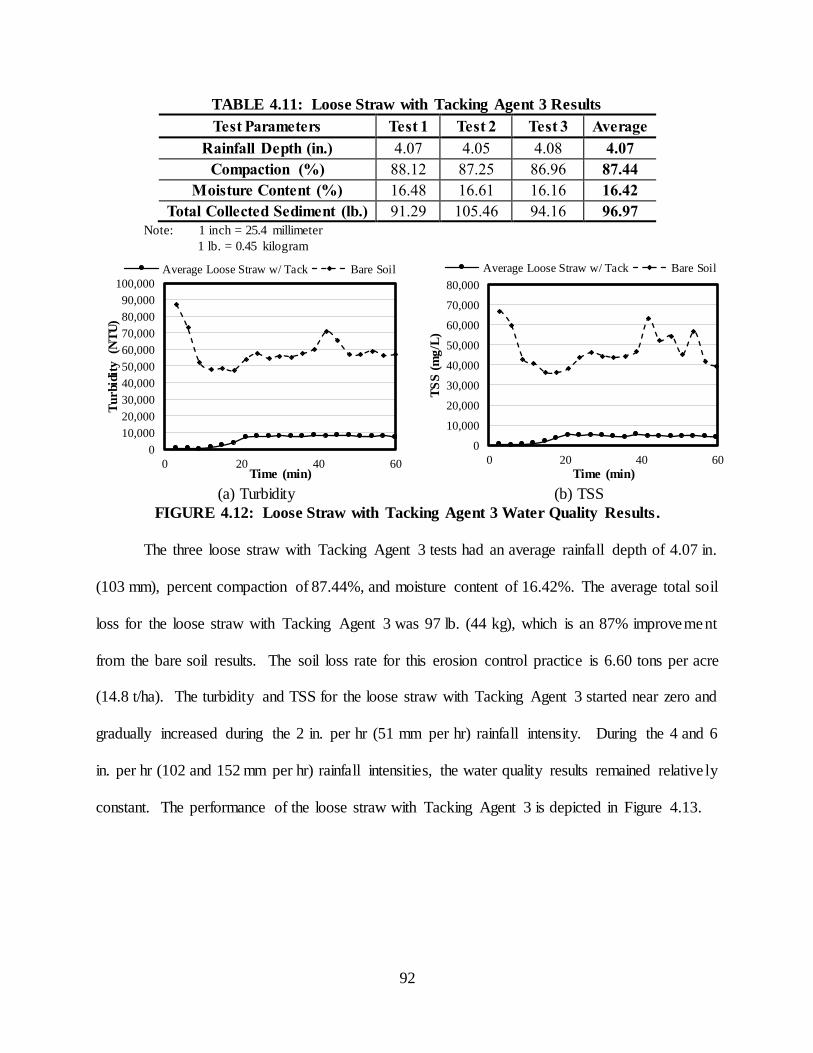
92
TABLE 4.11: Loose Straw with Tacking Agent 3 Results
Test Parameters Test 1 Test 2 Test 3 Average
Rainfall Depth (in.) 4.07 4.05 4.08 4.07
Compaction (%) 88.12 87.25 86.96 87.44
Moisture Content (%) 16.48 16.61 16.16 16.42
Total Collected Sediment (lb.) 91.29 105.46 94.16 96.97 Note: 1 inch = 25.4 millimeter
1 lb. = 0.45 kilogram
(a) Turbidity (b) TSS
FIGURE 4.12: Loose Straw with Tacking Agent 3 Water Quality Results.
The three loose straw with Tacking Agent 3 tests had an average rainfall depth of 4.07 in.
(103 mm), percent compaction of 87.44%, and moisture content of 16.42%. The average total soil
loss for the loose straw with Tacking Agent 3 was 97 lb. (44 kg), which is an 87% improvement
from the bare soil results. The soil loss rate for this erosion control practice is 6.60 tons per acre
(14.8 t/ha). The turbidity and TSS for the loose straw with Tacking Agent 3 started near zero and
gradually increased during the 2 in. per hr (51 mm per hr) rainfall intensity. During the 4 and 6
in. per hr (102 and 152 mm per hr) rainfall intensities, the water quality results remained relative ly
constant. The performance of the loose straw with Tacking Agent 3 is depicted in Figure 4.13.
0
10,000
20,000
30,000
40,000
50,000
60,000
70,000
80,000
90,000
100,000
0 20 40 60
Tu
rbid
ity
(NT
U)
Time (min)
Average Loose Straw w/ Tack Bare Soil
0
10,000
20,000
30,000
40,000
50,000
60,000
70,000
80,000
0 20 40 60
TS
S (
mg
/L)
Time (min)
Average Loose Straw w/ Tack Bare Soil

93
(a) Pre-test (b) 20 minute
(c) 40 minute (d) Post-test
FIGURE 4.13: Loose Straw with Tacking Agent 3 Test Photos.
4.4.4 Crimped Straw
Wheat straw was installed on the test plot at an application rate of 2 tons per acre (4.5 t/ha).
Following this application, the straw was imbedded into the soil a minimum of 2 in. (5.1 cm) with
a crimper. The straw was crimped every 8 in. (20.3 cm) perpendicular to the direction of flow.
The results of the crimped straw is depicted in Table 4.12 and Figure 4.14.

94
TABLE 4.12: Crimped Straw Test Results
Test Parameters Test 1 Test 2 Test 3 Average
Rainfall Depth (in.) 4.05 4.05 4.13 4.08
Compaction (%) 88.40 89.36 87.35 88.37
Moisture Content (%) 14.65 14.89 11.57 13.70
Total Collected Sediment (lb.) 187 175 142 168 Note: 1 inch = 25.4 millimeter
1 lb. = 0.45 kilogram
(a) Turbidity (b) TSS
FIGURE 4.14: Crimped Straw Water Quality Results.
The crimped straw tests resulted in an average rainfall depth of 4.08 in. (104 mm), an
average percent compaction of 88.37%, and an average moisture content of 13.70%. The average
soil loss for the three crimped straw tests was 168 lb. (76.2 kg), which is a 77% improvement from
the bare soil results. The crimped straw had a soil loss rate of 11.43 ton per acre (25.6 t/ha). The
turbidity and TSS results for the crimped straw quickly increased at the beginning of the
experiment to a consistent value throughout the remainder of the experiment. The crimped straw
had the worst water quality performance out of the three straw mulch applications under init ia l
product testing. This was most likely due to the process of imbedding the straw into the soil.
When imbedding the straw, the soil is disturbed resulting in loose soil on the test plot surface and
voids along the crimped straw. The performance of the crimped straw is depicted in Figure 4.15.
0
10,000
20,000
30,000
40,000
50,000
60,000
70,000
80,000
90,000
100,000
0 20 40 60
Tu
rbid
ity
(NT
U)
Time (min)
Average Crimped Straw Bare Soil
0
10,000
20,000
30,000
40,000
50,000
60,000
70,000
80,000
0 20 40 60
TS
S(m
g/L
)
Time (min)
Average Crimped Straw Bare Soil

95
(a) Pre-test (b) 20 minute
(c) 40 minute (d) Post-test
FIGURE 4.15: Crimped Straw Test Photos.
4.4.5 Straw Mulch Longevity Testing
Following the completion of the initial product performance tests, a longevity test was
performed on one of each of the straw mulch treatments to evaluate how well the straw mulch
practices will perform under multiple rainfall events. Between the initial and longevity
experiments, the test slope was not altered, the catch basin was cleaned out, and the water quality
samples were tested.
4.4.5.1 Bare Soil Longevity
Following the initial bare soil control test, a longevity experiment was performed on the
test plot to evaluate the performance of the bare soil under an additional rainfall event. There was

96
a two-day break between the initial and longevity experiments to allow for the completion of data
collection. The longevity bare soil had a rainfall depth of 4.12 in. (105 mm) and a total soil loss
of 611 lb. (277 kg). The longevity experiment experience a reduction in soil loss of 17% from the
initial bare soil control test. The water quality results of the experiment are depicted in Figure
4.16.
(a) Turbidity (b) TSS
FIGURE 4.16: Bare Soil Longevity Water Quality Results.
The turbidity and TSS water quality curves for the longevity experiment resulted in lower
concentrations throughout the experiment than the initial bare soil control test. The testing results
of the bare soil longevity experiment is depicted in Figure 4.17.
(a) Pre-test (b) Post-test
FIGURE 4.17: Bare Soil Longevity Results.
0
20,000
40,000
60,000
80,000
100,000
0 20 40 60
Tu
rbid
ity
(NT
U)
Time (min)
Bare Soil Bare Soil Longevity
0
10,000
20,000
30,000
40,000
50,000
60,000
70,000
80,000
0 20 40 60
TS
S (
mg
/L)
Time (min)
Bare Soil Bare Soil Longevity

97
4.4.5.2 Loose Straw Longevity
Following the initial loose straw test and data collection, a longevity experiment was
performed on the loose straw application. The longevity experiment was used to evaluate the
performance of the straw mulch when exposed to an additional rainfall event. The loose straw
longevity experiment had a rainfall depth of 4.13 in. (105 mm). The soil loss and water quality
from the bare soil control test is depicted in Table 4.13 and Figure 4.18. Table 4.13 shows the
percent improvement for the initial and longevity loose straw experiments as compared to the
corresponding initial and longevity bare soil control soil loss results.
TABLE 4.13: Loose Straw Longevity Soil Loss Results
Product Soil Loss (lb) Soil Loss Ratio % Improvement
Bare Soil Control 738 - - Bare Soil Longevity 611 - -
Loose Straw 143 0.19 81%
Loose Straw Longevity 287 0.47 53% Note: 1 lb. = 0.45 kilograms
(a) Turbidity (b) TSS
FIGURE 4.18: Loose Straw Longevity Water Quality Results.
The loose straw longevity test had a soil loss of 287 lb. (130 kg), which is double the soil
loss of the initial loose straw test of 143 lb. (64.9 kg). The longevity test resulted in a percent
improvement from the bare soil longevity test of 53%. The turbidity and TSS water quality
concentrations gradually increased throughout the rainfall experiment, while the initial loose straw
0
10,000
20,000
30,000
40,000
50,000
60,000
70,000
80,000
90,000
100,000
0 20 40 60
Tu
rbid
ity
(NT
U)
Time (min)
Loose Straw Loose Straw Longevity
0
10,000
20,000
30,000
40,000
50,000
60,000
70,000
80,000
0 20 40 60
TS
S (
mg
/L)
Time (min)
Loose Straw Loose Straw Longevity

98
test resulted in more constant values throughout most of the experiment. The loose straw was
washed from the test plot causing a larger amount of erosion to occur during the longevity test.
The loose straw longevity test plot conditions are depicted in Figure 4.19.
(a) Pre-Test (b) Post-Test
FIGURE 4.19: Loose Straw Longevity Photos.
4.4.5.3 Loose Straw with Tacking Agent 3
Following the initial test of the loose straw with Tacking Agent 3, a longevity test was
performed to determine the effectiveness of the straw anchoring application under an additiona l
rainfall event. The loose straw with Tacking Agent 3 longevity test had a rainfall depth of 4.12 in.
(105 mm). The soil loss from the initial and longevity test as well as the water quality results are
depicted in Table 4.14 and Figure 4.20.
TABLE 4.14: Loose Straw with Tacking Agent 3 Longevity Results
Product Soil Loss (lb.)
(lb)
Soil Loss
Ratio
% Improvement
Bare Soil Control 738 - - Bare Soil Longevity 611 - -
Loose Straw with Tackifier 97 0.13 87%
Loose Straw w/ Tackifier Longevity 131 0.21 79% Note: 1 lb. = 0.45 kilograms

99
(a) Turbidity (b) TSS
FIGURE 4.20: Loose Straw with Tacking Agent 3 Longevity Water Quality Results .
The loose straw with Tacking Agent 3 longevity experiment resulted in a total soil loss of
131 lb. (59.4 kg), while the initial test had a soil loss of 97 lb. (44 kg). The longevity test had a
percent improvement from bare soil conditions of 79%. The increase in soil loss is possibly due
to the tackifier washing from the test plot along with the straw cover. The turbidity and TSS water
quality concentrations were slightly better than the initial test. The turbidity values were consistent
throughout the entire experiment while the TSS values gradually increased during the 2 in. per hr
(51 mm per hr) rainfall intensity and became relatively constant for the remainder of the
experiment. The loose straw with Tacking Agent 3 performance is depicted in Figure 4.21.
(a) Pre-test (b) Post-test
FIGURE 4.21: Loose Straw with Tacking Agent 3 Longevity Photos.
0
10,000
20,000
30,000
40,000
50,000
60,000
70,000
80,000
90,000
100,000
0 20 40 60
Tu
rbid
ity
(NT
U)
Time (min)
Tacked Straw Tacked Straw Longevity
0
10,000
20,000
30,000
40,000
50,000
60,000
70,000
80,000
0 20 40 60
TS
S (
mg
/L)
Time (min)
Tacked Straw Tacked Straw Longevity

100
4.4.5.4 Crimped Straw Longevity
Following the completion of the initial crimped straw test, longevity testing was performed
on the crimped straw to determine the installations effectiveness under an additional rainfall event.
The crimped straw longevity test had a total rainfall depth of 4.07 in. (103 mm). The total soil loss
and water quality curves from the crimped straw longevity test are depicted in Table 4.15 and
Figure 4.22.
TABLE 4.15: Crimped Straw Longevity Results
Product Soil Loss (lb.) Soil Loss
Ratio
% Improvement
Bare Soil Control 738 - - Bare Soil Longevity 611 - -
Crimped Straw 169 0.23 77%
Crimped Straw Longevity 82 0.13 87% Note: 1 lb. = 0.45 kilograms
(a) Turbidity (b) TSS
FIGURE 4.22: Crimped Straw Longevity Water Quality Results.
The crimped straw longevity experiment had a total soil loss of 82 lb. (37.2 kg), while the
initial crimped straw test had a total soil loss of 169 lb. (77 kg). The longevity crimped straw had
an 87% improvement from the longevity bare soil results. The turbidity and TSS concentration
curves were greatly reduced from the initial crimped straw test. The turbidity and TSS values were
consistent throughout the entire rainfall event even though the rainfall intensity was increasing.
The substantial improvement from the initial to longevity testing is likely caused by the removal
0
10,000
20,000
30,000
40,000
50,000
60,000
70,000
80,000
90,000
100,000
0 20 40 60
Tu
rbid
ity
(NT
U)
Time (min)
Crimped Straw
Crimped Straw Longevity
0
10,000
20,000
30,000
40,000
50,000
60,000
70,000
80,000
0 20 40 60
TS
S (
mg
/L)
Time (min)
Crimped Straw Crimped Straw Longevity

101
of the disturbed soil during the first rainfall event caused by crimping the soil and filling the voids
around the crimped straw. As the longevity test continued, a tier system formed between the
crimped sections of straw. The tiers slowed down the flow of the runoff, which also reduced the
impact of the raindrops. The performance of the crimped straw during longevity experiments is
depicted in Figure 4.23.
(a) Pre-test (b) Post-test
FIGURE 4.23: Crimped Straw Longevity Photos.
Due to the substantial improvement between the initial and longevity tests of the crimped
straw, additional longevity tests were performed. The second longevity test had a total rainfa ll
depth of 4.07 in. (103 mm) with a total soil loss of 78 lb. (35.4 kg). The third longevity experiment
had a total rainfall depth of 4.02 in. (102 mm) with a total soil loss of 83 lb. (37.6 kg). The turbidity
and TSS water quality curves for the longevity experiments are depicted in Figure 4.24.

102
(a) Turbidity (b) TSS
FIGURE 4.24: Crimped Straw Longevity Results.
The first and second longevity experiments followed similar turbidity and TSS
concentration curves while the third longevity experiment showed an improvement in water
quality results. The improvement in performance was potentially caused by the formation of a tier
system between the rows of crimped straw. The tier formation occurring with the crimped straw
is depicted in Figure 4.25. Another potential cause of improvement was that the three prior rainfa ll
events had removed a majority of the fine, easily erodible surface soils causing a reduction in the
amount of soil eroding from the slope. All three of the longevity experiments had a near zero
initial turbidity concentrations and quickly increased to a concertation that was relatively constant
for the remainder of the experiment.
0
10,000
20,000
30,000
40,000
50,000
60,000
70,000
80,000
90,000
100,000
0 20 40 60
Tu
rbid
ity
(NT
U)
Time (min)
Longevity 1 Longevity 2 Longevity 3
0
10,000
20,000
30,000
40,000
50,000
60,000
70,000
80,000
0 20 40 60
TS
S (
mg
/L)
Time (min)
Longevity 1 Longevity 2 Longevity 3

103
FIGURE 4.25: Crimped straw tier formation
4.4.6 Straw Mulch Statistical Analysis
A statistical analysis was performed on the initial straw mulch results to determine if any
of the straw mulch applications had statistically similar soil loss results. An ANOVA test was
performed to determine if the means of all three straw mulch applications soil loss results were
equal. If the p-value resulting from the ANOVA test was less than the alpha value of 0.05, then
the null hypothesis that all three means were equal would be rejected. The results from the
ANOVA test are summarized in Table 4.16.
TABLE 4.16: Straw Mulch ANOVA Results
Degrees of
Freedom Alpha Value F-value p-value
9 0.05 8.444 0.014
The ANOVA test resulted in a p-value less than the alpha value of 0.05. Therefore, the
null hypothesis that all three of the means was equal was rejected. At least one of the straw mulch
soil loss means was statistically different from the others. Three hypothesis tests was performed
to compare the loose versus tackifier, loose versus crimped, and the tackifier versus crimped straw
to determine which means were equal. The hypothesis tested for this statistical analysis is depicted
in Equation 4.1 and 4.2. The null hypothesis of this experiment was that the two sample means
were statistically equal, while the alternative hypothesis was that the means were not equal. If the

104
p-value resulting from the hypothesis test is less than 0.05, then the alternative hypothesis is true.
The results from the three hypothesis tests is summarized in Table 4.17.
𝐻0: 𝜇1 = 𝜇2 (4.1) where,
H0 = null hypothesis µ1 = variable one mean
µ2 = variable two mean
𝐻1: 𝜇1 ≠ 𝜇2 (4.2) where,
H1 = alternative hypothesis µ1 = variable one mean
µ2 = variable two mean
TABLE 4.17: Straw Mulch Hypothesis Test
Hypothesis Test Application 1
Mean (lb.)
Application 2
Mean Alpha Value p-value
Loose vs. Tackifier 143 97 0.05 0.042
Loose vs. Crimped 143 168 0.05 0.185
Tackifier vs. Crimped 97 168 0.05 0.002
Note: 1 lb. = 0.45 kilograms
The loose versus tackifier and the tackifier versus crimped straw hypothesis tests resulted
in p-values that were less than the alpha value of 0.05. Therefore, the null hypothesis was rejected,
resulting in the means between the two initial straw applications soil loss results not being equal.
The loose versus crimped straw hypothesis test resulted in a p-value greater than 0.05. Therefore,
the means between these two initial straw applications soil loss results was equal. The straw with
tackifier soil loss for the initial product test was statistically different from the other two straw
mulch applications under initial product testing.
4.4.7 Straw Summary
Three straw mulching applications were evaluated under the AU-ESCTF rainfall simula tor
to compare the erosion control practice performance to bare soil control tests on a sandy loam soil.
The straw mulch was installed as a loose straw, loose straw with Tacking Agent 3, and crimped

105
straw. The turbidity of the test plot runoff is summarized for each straw mulch application and the
bare soil control tests in Figure 4.26 and the soil loss for each application is summarized Table
4.18.
TABLE 4.18: Straw Mulch Soil Loss Results
Product Soil Loss (lb.) Soil Loss Ratio % Improvement
Bare Soil Control 738 - - Loose Straw 143 0.19 81%
Loose Straw with Tacking Agent 3 97 0.13 87%
Crimped Straw 169 0.23 77%
Note: 1 lb. = 0.45 kilograms
FIGURE 4.26: Straw Mulch Turbidity Summary.
All three of the straw applications showed substantial reduction in turbidity throughout the
entire experiment. The best performing straw application under initial performance testing was
the loose straw with Tacking Agent 3 with a total soil loss of 97 lb. (44 kg), which was an 87%
improvement from bare soil conditions. The crimped straw was the worst performing straw mulch
application under initial product performance testing. The crimped straw had a total soil loss of
169 lb. (76.6 kg), which was a 77% improvement from bare soil conditions. The test plot
conditions following the initial product test is depicted in Figure 4.27.
0
10,000
20,000
30,000
40,000
50,000
60,000
70,000
80,000
90,000
100,000
0 10 20 30 40 50 60
Tu
rbid
ity (
NT
U)
Time (min)
Bare Soil Loose Straw Loose Straw w/ tack Loose Straw Crimped

106
(a) Bare soil (b) Loose straw
(c) Loose straw with Tacking Agent 3 (d) Crimped straw
FIGURE 4.27: Straw Mulch Product Results.
The straw mulch applications and bare soil were exposed to a second rainfall event to
evaluate the longevity performance of the erosion control applications. The soil loss results for
the second rainfall event and the water quality curves are depicted in Table 4.19 and Figure 4.28.
TABLE 4.19: Straw Mulch Longevity Soil Loss
Product Soil Loss (lb.) Soil Loss Ratio % Improvement
Bare Soil Control 611 - - Loose Straw 287 0.47 53%
Loose Straw with Tacking Agent 3 131 0.21 79%
Crimped Straw 82 0.13 87% Note: 1 pound = 0.45 kilograms

107
FIGURE 4.28: Straw Mulch Longevity Water Quality Results.
The longevity testing of the straw mulch applications resulted in different results from the
initial product testing. Unlike in the initial test, the crimped straw was the best performing straw
mulch application with a total soil loss of 82 lb. (37.2 kg), which is an 87% improvement from the
longevity bare soil results. The crimped straw and the loose straw with Tacking Agent 3 had
similar turbidity measurements throughout the duration of the longevity experiments. The loose
straw was the worst performing straw mulch application with a total soil loss of 287 lb. (130.2 kg),
which is a 53% improvement from bare soil conditions. The loose straw with Tacking Agent 3
did not perform as well under longevity testing as under initial product testing. The total soil loss
for the loose straw with tackifier under longevity testing was 131 lb. (59.4 kg), which is a 79%
improvement from the bare soil conditions. The reason for the drop off in performance of the
loose straw with tackifier is likely caused by the tackifier being washed from the test plot. The
crimped straw had an increased performance because the loose soil that was disturbed by the
0
10,000
20,000
30,000
40,000
50,000
60,000
70,000
80,000
90,000
100,000
0 10 20 30 40 50 60
Tu
rbid
ity
(NT
U)
Time (min)
Bare Soil Loose Straw Loose Straw w/ tack
Loose Straw Crimped Bare Soil Longevity

108
crimping process had been washed form the site and the voids caused by the crimper had been
filled with sediment.
The initial and longevity soil loss results were combined to determine the overall
effectiveness of each straw mulch application. The soil loss data for the combined results is
depicted in Table 4.20.
TABLE 4.20: Combined Straw Mulch Results
Straw Application Combined Soil Loss (lb.) Soil Loss Ratio % Improvement
Bare Soil 1,349 - -
Loose Straw 430 0.32 68%
Loose Straw w/ Tackifier 228 0.17 83%
Crimped Straw 251 0.19 81%
Note: 1 lb. = 0.45 kilograms
The combination of the initial and longevity results shows that anchoring straw reduces the
amount of erosion. The loose straw with Tacking Agent 3 was the best performing straw mulch
practice with an 83% improvement from the bare soil conditions. The crimped straw was the
second best straw application with an 81% improvement from bare soil conditions. The crimped
straw and loose straw with Tacking Agent 3 were similar in performance with only a 23 lb. (10.4
kg) difference in combined soil loss. The loose straw application resulted in a 68% improvement
from bare soil conditions. The results found in this study prove that anchored straw applications
provided the greatest erosion reduction occurring on steep slopes.
4.5 HYDRAULIC MULCH RESULTS
At the conclusion of straw mulch testing, the rainfall simulator slope was rebuilt and a new
loam soil was used for constructing the slope to meet ASTM D6459-19. The loam soil was then
used to determine the performance of three hydraulic mulch products as compared to bare soil
control tests. The three types of hydraulic mulches were Eco-Fibre plus Tackifier, Soil Cover
Wood Fiber with Tack, and Terra-Wood with Tacking Agent 3. The data collected for each
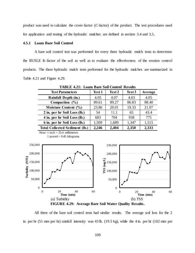
109
product was used to calculate the cover-factor (C-factor) of the product. The test procedures used
for application and testing of the hydraulic mulches are defined in section 3.4 and 3.5.
4.5.1 Loam Bare Soil Control
A bare soil control test was performed for every three hydraulic mulch tests to determine
the RUSLE K-factor of the soil as well as to evaluate the effectiveness of the erosion control
products. The three hydraulic mulch tests performed for the hydraulic mulches are summarized in
Table 4.21 and Figure 4.29.
TABLE 4.21: Loam Bare Soil Control Results
Test Parameters Test 1 Test 2 Test 3 Average
Rainfall Depth (in.) 4.05 4.07 4.03 4.05
Compaction (%) 89.61 89.27 86.83 88.40
Moisture Content (%) 23.86 20.01 19.33 21.07
2 in. per hr Soil Loss (lb.) 54 11.1 65 43.4
4 in. per hr Soil Loss (lb.) 683 704 938 775
6 in. per hr Soil Loss (lb.) 1,509 1,689 1,347 1,515
Total Collected Sediment (lb.) 2,246 2,404 2,350 2,333
Note: 1 inch = 25.4 millimeters
1 pound = 0.45 kilograms
(a) Turbidity (b) TSS
FIGURE 4.29: Average Bare Soil Water Quality Results.
All three of the bare soil control tests had similar results. The average soil loss for the 2
in. per hr (51 mm per hr) rainfall intensity was 43 lb. (19.5 kg), while the 4 in. per hr (102 mm per
0
50,000
100,000
150,000
200,000
250,000
0 20 40 60
Tu
rbid
ity
(NT
U)
Time (min)
0
50,000
100,000
150,000
200,000
250,000
0 20 40 60
TS
S (
mg
/L)
Time (min)

110
hr) rainfall intensity had an average soil loss of 775 lb. (352 kg). There was a large increase in
soil loss between the 2 and 4 in. per hr (51 and 102 mm per hr) rainfall intensities. This is evident
when reviewing the turbidity and TSS data. The 2 in. per hr (51 mm per hr) rainfall intensity water
quality measurements gradually increases, but when the 4 in. per hr (102 mm per hr) rainfa ll
intensity started, the turbidity and TSS values increased quickly. The average total soil loss for
the loam soil was 2,333 lb. (1,058 kg), which is substantially more soil loss than the sandy loam
soil. The performance of the loam soil under bare soil control conditions is depicted in Figure
4.30.
(a) Pre-test (b) 20 minute
(c) 40 minute (d) Post-test
FIGURE 4.30: Loam Bare Soil Test Results.

111
4.5.1.1 K-factor Results
The bare soil control results were used to calculate the K-factor for the loam soil. The soil
loss and the rainfall depth following each twenty-minute testing segment was used to calculate the
K-factor. The K-factor was later used to determine the C-factor for each erosion control product.
The RUSLE values used to determine the K-factor for the three bare soil control tests are
summarized in Table 4.22.
TABLE 4.22: Bare Soil RUSLE Data
Bare Soil
Control Test
for each
Product
Rainfall Intensity (in.
per hr)
Cumulative
R
Cumulative
A (ton per
acre)
Eco Fiber -
Plus
2 12.01 3.66
4 60.41 50.14
6 188.88 152.85
Soil Cover
2 13.20 0.75
4 64.23 47.88
6 184.62 162.89
Terra-Wood
2 13.20 4.42
4 61.54 68.25
6 182.11 159.96 Note: 1 inch per hour = 25.4 millimeters per hour
This data was used to plot the soil loss (A) versus the R-factor. A linear equation was fitted
to the data set and the equation was used to calculate the soil loss for the theoretical R-factor value
of 182.02. The theoretical R-factor was calculated using the drop size distribution data collected
using the flour pan method in section 3.2.1. The linear trend line and equation are depicted in
Figure 4.31.

112
FIGURE 4.31: K-Factor Regression Equation.
The soil loss value that coordinates with the theoretical R-factor of 182.02 on the linear
regression equation was 159.21 ton per acre (357 t/ha). The RUSLE equation was used to quantify
the K-factor using the data shown in Table 4.23.
TABLE 4.23: K-factor Calculations
A = 159.21
Theoretical R = 182.02
LS = 2.86
C = 1.0
P = 1.0
K = 0.311
Since the test plot is bare soil, the C-factor and P-factor are 1.0. The K-factor of the loam
soil determined for the hydraulic mulch bare soil control tests was 0.31.
4.5.2 Eco-Fibre plus Tackifier
Profile Products Eco-Fibre plus Tackifier (Eco-Fibre) is a hydraulic mulch product
consisting of 85% thermally refined wood fibers, 3% polymer based tackifier, and 12% moisture
content. Eco-Fibre’s manufacturer data sheet can be found in Appendix B. The product was
installed on the test slope at an application rate of 2,500 lb. per acre (2,802 kg per ha). Eco-Fibre
y = 0.8886x - 4.7237
R² = 0.9859
0
20
40
60
80
100
120
140
160
180
0 20 40 60 80 100 120 140 160 180 200
A(t
on/a
c)
R-factor

113
was evaluated three times under rainfall simulation and compared to a bare soil control test. The
test results for the Eco-Fibre hydraulic mulch is summarized in Table 4.24 and Figure 4.32.
TABLE 4.24: Eco-Fibre plus Tackifier Test Results
Test Parameters Bare Soil
Control Test 1 Test 2 Test 3 Average
Rainfall Depth (in.) 4.05 4.10 4.04 3.97 4.04
Compaction (%) 89.61 85.81 87.97 88.17 87.32
Moisture Content (%) 23.86 26.07 16.65 22.75 21.82
2 in. per hr Soil Loss (lb.) 54 2.43 3.57 4.36 3.45
4 in. per hr Soil Loss (lb.) 683 356 377 279 337
6 in. per hr Soil Loss (lb.) 1,509 734 1,220* 700 717
Total Collected Sediment (lb.) 2,246 1,092 1,601* 984 1,038
Note: *A storm event occurred following the test removing the slope cover and washing add itional soil into
the catch basin affecting the 6 in. per hr (152 mm per hr) soil loss.
1 inch = 25.4 millimeters
1 pound = 0.45 kilograms
(a) Turbidity (b) TSS
FIGURE 4.32: Eco-Fibre plus Tackifier Water Quality Results.
The Eco-Fiber plus Tackifier had an average soil loss of 1,038 lbs. (471 kg), while the bare
soil control test had a total soil loss of 2,246 lb. (1,019 kg). The installation of the hydraulic mulch
resulted in a 54% improvement from the bare soil conditions. The hydraulic mulch was effective
during the 2 in. per hr (51 mm per hr) rainfall intensity. The turbidity and TSS measurements were
near zero for the first 20 minutes of the experiment, but soon after the 4 in. per hr (102 mm per hr)
rainfall intensity started, the hydraulic mulch began to wash from the test slope. Therefore, the
0
50,000
100,000
150,000
200,000
250,000
300,000
0 20 40 60
Tu
rbid
ity
(NT
U)
Time (min)
Bare Soil Average EcoFibre
0
50,000
100,000
150,000
200,000
250,000
300,000
0 20 40 60
TS
S (
mg
/L)
Time (min)
Bare Soil Average EcoFibre

114
turbidity and TSS measurements substantially increased. Even though a large portion of the
hydraulic mulch was washed from the test plot, the turbidity and TSS measurements were still less
than the corresponding bare soil conditions. Following Eco-Fibre test 2, a natural rainfall event
occurred, removing the test plot cover and causing erosion. The 6 in. per hr (152 mm per hr) soil
loss data was effected by the erosion that occurred from the post-test rainfall event. The
performance of the hydraulic mulch is depicted in Figure 4.33.
(a) Pre-test (b) 20 minute
(c) 40 minute (d) Post-test
FIGURE 4.33: Eco-Fibre plus Tackifier Test Photos.
4.5.2.1 Eco-Fibre plus Tackifier C-factor
Following the completion of the three Eco-Fibre plus Tackifier, tests and a bare soil control
test, the C-factor for the product was calculated using the soil loss, rain gauge measurements, and

115
the drop size distribution data. Before the C-factor could be calculated, the K-factor for the
corresponding bare soil control test must be determined. The soil loss (A) and R-factor for each
rainfall intensity were plotted to determine a linear equation. The K-factor calculation of the bare
soil control is depicted in Figure 4.34.
FIGURE 4.34: Eco-Fibre K-Factor Trendline Equation from Bare Soil Control Test.
The three data points were the resulting values from the 2, 4, and 6 in. per hr (52, 102, and
152 mm per hr) rainfall intensities for A and R-factor. The linear equation that best fits the three
data points was used to determine the soil loss that corresponds with the theoretical R-factor. The
RUSLE equation was solved for the K-factor. Since the bare soil control test was used to calculate
the K-factor, the C-factor and P-factor were both 1.0 and an LS-factor of 2.86. The A-factor
calculated from the regression equation was 148.08 tons per acre (332 t/ha) for a theoretical R-
factor of 182.02. The resulting K-factor for the Eco-Fibre plus Tackifier tests was 0.29.
Once the K-factor for the Eco-Fibre test group was calculated, the product C-factor was
determined. The rainfall depth and soil loss data collected for each rainfall intensity was used to
calculate the A-factor for each product test that corresponds with the theoretical R-factor of 182.02.
The Eco-Fibre tests resulted in A-factors of 74.34, 180.95, and 66.96 tons per acre (166.64, 405.63,
and 150.10 t/ha). The C-factor for the product was calculated using two different procedures. The
y = 0.8344x - 3.7924
R² = 0.9983
0
20
40
60
80
100
120
140
160
180
0 20 40 60 80 100 120 140 160 180 200
A(t
on/a
c)
R-factor

116
first method plotted the incremental C-factor from actual soil loss versus the incremental R-factor,
which is depicted in Figure 4.35.
FIGURE 4.35: Eco-Fibre C-factor Equation.
A linear trendline was fit to the data points from the 2, 4, and 6 in. per hr (51, 102, and 152
mm per hr) rainfall intensities. The C-factor corresponding with the theoretical R-factor of 182.02
was calculated using the trendline equation. The resulting C-factor for this method was 0.596.
Since the 2 in. per hr (51 mm per hr) C-factor was much smaller than the 4 and 6 in. per hr (102
and 152 mm per hr) C-factors, a statistical analysis was performed to determine if the mean of the
C-factors were equal. Hypothesis tests were performed on the C-factor data for each rainfa ll
intensity for the Eco-Fibre test results in section 4.5.2.2. Since the means of the 2-4 in. per hr (51-
102 mm per hr) and 2-6 in. per hr (51-152 mm per hr) hypothesis tests were not equal, the 2 in.
per hr (51 mm per hr) C-factor value was not used in this method to determine the product C-
factor. The 2 in. per hr (51 mm per hr) C-factor was negligible compared to the 4 and 6 in. per hr
(102 and 152 mm per hr) C-factors and therefore was biasing in the regression equation. The C-
factor calculations without the 2 in. per hr (51 mm per hr) data is depicted in Figure 4.36.
y = 0.0026x + 0.1223
0.0
0.2
0.4
0.6
0.8
1.0
0 50 100 150 200
C-
fact
or
R-factor

117
FIGURE 4.36: Eco-Fibre C-factor Equation without 2 in. per hr Data.
Since the slope of the trendline is nearly zero, then the C-factor between the 4 and 6 in. per
hr (102 and 152 mm per hr) rainfall events provide a more uniform C-factor between storm events,
which should be achieved since C-factor is not considered storm dependent. The regression
equation was used to calculate average C-factor for all three experiments using the theoretical R-
factor of 182.02. The C-factor using the first method was 0.551. The second method averaged
the A-factors from the three Eco-Fibre experiments and inserted the average A-factor into the
RUSLE equation. The C-factor calculation for the second method is depicted in Table 4.25.
TABLE 4.25: Eco-Fibre RUSLE Calculations
A = 83.42
Theoretical R = 182.02
LS= 2.86
K = 0.29
P = 1.0
C = 0.5493
The resulting C-factor from the second method was 0.549. Therefore, the two C-factor
calculation procedures used resulted in C-factor values of 0.551 and 0.549 for the Eco-Fibre with
Tackifier hydraulic mulch. When using the 2 in. per hr (51 mm per hr) C-factor data for the first
method, the resulting C-factor was 0.596. When the 2 in. per hr (51 mm per hr) C-factor data was
y = 0.0007x + 0.4238
0.0
0.2
0.4
0.6
0.8
1.0
0 50 100 150 200
C-f
act
or
R-factor

118
not included, the C-factor value was nearly equal to the second method. Therefore, the 2 in. per
hr (51 mm per hr) C-factor data skews the data resulting in inaccurate results.
4.5.2.2 Eco-Fibre plus Tackifier Statistical Analysis
Three hypothesis tests were performed on the incremental C-factor calculated for the three
Eco-Fibre plus Tackifier experiments. The three hypothesis tests compared the 2-4 in. per hr (51-
102 mm per hr), 2-6 in. per hr (51-152 mm per hr), and the 4-6 in. per hr (102-152 mm per hr)
rainfall intensity C-factor results to determine if the means of the resulting C-factors were equal.
If the two-tail p-value was less than the alpha value of 0.05, then the null hypothesis was rejected,
concluding that the means of the two rainfall intensity C-factors are not equal. The hypothesis
used to evaluate whether the 2, 4, and 6 in. per hr (51, 102, and 152 mm per hr) C-factors were
equal for all of the erosion control practices is depicted in Equation 4.3 and 4.4. The null
hypothesis of this experiment was that the two sample means were statistically equal, while the
alternative hypothesis was that the means were not equal. If the hypothesis test resulted in a p-
value less than 0.05, then the null hypothesis was rejected. The results from the three hypothesis
tests for the Eco-Fibre plus Tackifier are depicted in Table 4.26.
𝐻0: 𝜇1 = 𝜇2 (4.3) where, H0 = null hypothesis
µ1 = variable one mean
µ2 = variable two mean
𝐻1: 𝜇1 ≠ 𝜇2 (4.4) where,
H1 = alternative hypothesis µ1 = variable one mean
µ2 = variable two mean

119
TABLE 4.26: Eco-Fibre plus Tackifier Hypothesis Test Results
Hypothesis
Test
Intensity 1
Mean
Intensity 2
Mean Alpha p (two-tail)
2-4 in. per hr 0.0213 0.4655 0.05 0.006
2-6 in. per hr 0.0213 0.5456 0.05 0.023
4-6 in. per hr 0.4655 0.5456 0.05 0.432
The 2-4 in. per hr (51-102 mm per hr) and 2-6 in. per hr (51-152 mm per hr) hypothesis
tests resulted in p-values less than the alpha value of 0.05. Therefore, the null hypothesis was
rejected, concluding that the means, which represent the RUSLE C-values calculated for each
intensity, are not equal. The 4-6 in. per hr (102-152 mm per hr) hypothesis test resulted in a p-
value greater than 0.05, concluding that the null hypothesis was accepted and that the means are
equal.
4.5.3 Soil Cover Wood Fiber with Tack
Soil Cover Wood Fiber with Tack (Soil Cover) is a hydraulic mulch consisting of 85%
thermally refined wood fibers, 3% polymer based tackifier, and 12% moisture content. Soil Covers
manufacturer data sheet can be found in Appendix B. Soil Cover was evaluated three times at an
application rate of 2,500 lb. per acre (2,802 kg per ha). All three of the hydraulic mulch
experiments were compared to a bare soil control test. The Soil Cover test results are summarized
in Table 4.27 and Figure 4.37.
TABLE 4.27: Soil Cover Wood Fiber with Tack Test Results
Test Parameters Bare Soil
Control Test 1 Test 2 Test 3 Average
Rainfall Depth (in.) 4.07 4.01 4.05 4.07 4.04
Compaction (%) 89.27 86.29 88.39 87.98 87.55
Moisture Content (%) 20.01 18.18 21.27 21.73 20.39
2 in. per hr Soil Loss (lb.) 11.1 0 6.60 1.40 2.67
4 in. per hr Soil Loss (lb.) 704 304 410 433 382
6 in. per hr Soil Loss (lb.) 1,689 841 634 861 779
Total Collected Sediment (lb.) 2,405 1,145 1,051 1,296 1,164
1 inch = 25.4 millimeters
1 pound = 0.45 kilograms

120
(a) Turbidity (b) TSS
FIGURE 4.37: Soil Cover Wood Fiber with Tack Water Quality Results.
Soil Cover had an average total soil loss of 1,164 lb. (528 kg), while the bare soil control
test had an average soil loss of 2,405 lb. (1,091 kg). The hydraulic mulch had a 52% reduction in
soil loss from the bare soil conditions. Soil Cover was most effective during the 2 in. per hr (51
mm per hr) rainfall event with an average soil loss of 2.67 lb. (1.21 kg) and low turbidity and TSS
measurements. However, soon after the 4 in. per hr (102 mm per hr) rainfall intensity started, the
hydraulic mulch began to wash off the test plot. The turbidity and TSS measurements substantia l ly
increased during the beginning of the 4 in. per hr (102 mm per hr) rainfall intensity as the hydraulic
mulch was washed from the test plot. Once some of the hydraulic mulch had washed off the test
plot, the soil loss greatly increased from 2.67 lb. (1.21 kg) during the 2 in. per hr (51 mm per hr)
test segment to an average of 382 lb. (173 kg) of soil loss during the 4 in. per hr (102 mm per hr)
test segment. The performance of the Soil Cover Wood Fiber with Tack is depicted in Figure 4.38.
0
50,000
100,000
150,000
200,000
250,000
300,000
0 20 40 60
Tu
rbid
ity
(NT
U)
Time (min)
Bare Soil Average Soil Cover
0
50,000
100,000
150,000
200,000
250,000
300,000
0 20 40 60
TS
S (
mg
/L)
Time (min)
Bare Soil Average Soil Cover

121
(a) Pre-test (b) 20 minute
(c) 40 minute (d) Post-test
FIGURE 4.38: Soil Cover Wood Fiber with Tack Test Photos.
4.5.3.1 Soil Cover Wood Fiber with Tack C-factor
Once the three Soil Cover tests and the bare soil control test data had been collected, the
soil loss, rainfall depth, and drop size distribution data were used to calculate the C-factor of the
hydraulic mulch. Prior to calculating the Soil Cover C-factor, the K-factor for the corresponding
bare soil control test was determined. The K-factor was calculated by plotting the A-factor in
tons/acre vs. the R-factor as depicted in Figure 4.39.

122
FIGURE 4.39: Soil Cover K-factor Trendline Equation.
The linear trendline equation was fitted to the three data points. The A-factor that
corresponds with the theoretical R-factor was equal to 160.21 tons per acre (359 t per ha). The
RUSLE Equation was used to calculate the K-factor using the theoretical R-factor, an LS-factor of
2.86, C-factor of 1.0, and the P-factor of 1.0. The resulting K-factor for the Soil Cover tests is
0.33.
The cumulative A-factor for each of the three Soil Cover rainfall experiments was 77.93,
71.50, and 88.18 tons per acre (174.7, 160.3, and 197.7 metric t/ha). There were two methods used
to calculate the C-factor of the Soil Cover hydraulic mulch. The first method plotted the
incremental C-factor calculated using the actual soil loss for each rainfall intensity versus the
incremental R-factor and is depicted in Figure 4.40. Three hypothesis tests were performed on the
C-factor data to determine if the C-factor means were equal in section 4.5.3.2. The hypothesis
tests concluded that the means were not equal for all three intensities. Since the 4-6 in. per hr
(102-152 mm per hr) C-factor means were equal, but the 2 in. per hr (51 mm per hr) C-factor mean
was not equal to the 4 or 6 in. per hr (102 or 152 mm per hr) C-factors. Since the 2 in. per hr (51
mm per hr) C-factor mean was not equal, the data was excluded from Figure 4.39 because it would
skew the results of the trend line equation.
y = 0.9475x - 12.264
R² = 0.9999
0
20
40
60
80
100
120
140
160
180
0 20 40 60 80 100 120 140 160 180 200
A(t
on/a
c)
R-factor

123
(a) Full test C-factor (b) Without 2 in. per hr C-factor
FIGURE 4.40: Soil Cover C-factor Equation.
The regression equation from Figure 4.40(b) was used to calculate the C-factor that
corresponded with the theoretical R-factor of 182.02. The C-factor calculated for the Soil Cover
hydraulic mulch was 0.454.
The second method used to calculate the C-factor for the Soil Cover hydraulic mulch
averaged the cumulative A-factor for each rainfall experiment. The average A-factor along with
the RUSLE variables were used to calculate the C-factor as depicted in Table 4.28.
TABLE 4.28: Soil Cover RUSLE Equation
A = 79.21
Theoretical R = 182.02
LS = 2.86
K = 0.33
P = 1.0
C = 0.4592
The C-factor calculated using the second method was 0.459. Therefore, the two methods
to calculate the C-factor of the Soil Cover Wood Fiber with Tack was 0.454 and 0.459.
4.5.3.2 Soil Cover Wood Fiber with Tack Statistical Analysis
Three hypothesis tests were performed on the incremental C-factors calculated for the three
Soil Cover experiments. The three hypothesis tests compared the 2-4 in. per hr (51-102 mm per
y = 0.002x + 0.1407
0.0
0.2
0.4
0.6
0.8
1.0
0 50 100 150 200
C-f
acto
r
R-factor
y = -1E-04x + 0.4721
0.0
0.2
0.4
0.6
0.8
1.0
0 50 100 150 200
C-f
acto
r
R-factor

124
hr), 2-6 in. per hr (51-152 mm per hr), and 4-6 in. per hr (102-152 mm per hr) rainfall intensity C-
factors to determine if the means of the each intensities C-factors were equal. If the two-tail p-
value was less than the alpha value of 0.05, then the null hypothesis was rejected, concluding that
the means of the two rainfall intensity C-factors are not equal. The results from the three
hypothesis tests for the Soil Cover experiments is depicted in Table 4.29.
TABLE 4.29: Soil Cover Hypothesis Test Results
Hypothesis
Test
Intensity 1
Mean
Intensity 2
Mean Alpha p (two-tail)
2-4 in. per hr 0.0144 0.4673 0.05 0.008
2-6 in. per hr 0.0144 0.4528 0.05 0.001
4-6 in. per hr 0.4673 0.4528 0.05 0.773
The 2 to 4 in. per hr (51 to 102 mm per hr) and 2 to 6 in. per hr (51 to152 mm per hr)
hypothesis tests resulted in p-values less than the alpha value of 0.05. Therefore, the null
hypothesis was rejected, concluding that the means are not equal. The 4 to 6 in. per hr (102 to 152
mm per hr) hypothesis test resulted in a p-value greater than 0.05, concluding that the null
hypothesis was accepted and that the means are equal. The 2 in. per hr (51 mm per hr) C-factors
were much smaller than the 4 and 6 in. per hr (102 and 152 mm per hr) C-factors, which
corresponds with the results of the hypothesis tests.
4.5.4 Terra-Wood with Tacking Agent 3
Terra-Wood with Tacking Agent 3 (Terra Wood) is a hydraulic mulch composed of 97%
thermally processed wood fibers and 3% polymer based tackifier. Terra-Woods manufacturer data
sheet can be found in Appendix B. The hydraulic mulch was installed at an application rate of
2,500 lb. per acre (2,802 kg per ha) and allowed to cure for a minimum of 24 hours prior to rainfa ll
simulation testing. The hydraulic mulch was evaluated with three rainfall simulation tests and
compared to the performance of a bare soil control test. The test results for the hydraulic mulch is
depicted in Table 4.30 and Figure 4.41.

125
TABLE 4.30: Terra-Wood with Tacking Agent 3 Test Results
Test Parameters Bare Soil
Control Test 1 Test 2 Test 3 Average
Rainfall Depth (in.) 4.03 4.07 4.07 4.03 4.06
Compaction (%) 86.83 88.36 87.00 87.04 87.47
Moisture Content (%) 19.33 21.22 19.79 17.64 19.55
2 in. per hr Soil Loss (lb.) 65 3.98 3.85 14.8 8.54
4 in. per hr Soil Loss (lb.) 938 296 686 483 491
6 in. per hr Soil Loss (lb.) 1,347 679 881 832 832
Total Collected Sediment (lb.) 2,350 979 1,574 1,330 1,294
Note: 1 inch = 25.4 millimeters
1 lb. = 0.45 kilograms
(a) Turbidity (b) TSS
FIGURE 4.41: Terra-Wood with Tacking Agent 3 Water Quality Results.
Terra-Wood had an average soil loss of 1,294 lb. (587 kg), while the bare soil control test
had a total soil loss of 2,350 lb. (1,066 kg). The hydraulic mulch reduced the amount of erosion
occurring during the experiment by 45%. Similar to the other hydraulic mulches, Terra-Wood was
effective during the 2 in. per hr (51 mm per hr) rainfall intensity with an average soil loss of 8.54
lb. (3.87 kg). However, once the rainfall intensity was increased to 4 in. per hr (102 mm per hr),
the hydraulic mulch began to wash from the test plot. The soil loss increased from 8.54 lb. (3.87
kg) during the 2 in. per hr (51 mm per hr) rainfall intensity to 491 lb. (222.7 kg) during the 4 in.
per hr (102 mm per hr) rainfall intensity. The turbidity and TSS measurements show that the
0
50,000
100,000
150,000
200,000
250,000
300,000
0 20 40 60
Tu
rbid
ity
(NT
U)
Time (min)
Bare Soil Average Terra Wood
0
50,000
100,000
150,000
200,000
250,000
300,000
0 20 40 60
TS
S (
mg
/L)
Time (min)
Bare Soil Average Terra Wood

126
concentration of the runoff substantially increased during the 4 in. per hr (102 mm per hr) rainfa ll
intensity. The performance of the hydraulic mulch is depicted in Figure 4.42.
(a) Pre-test (b) 20 minute
(c) 40 minute (d) Post-test
FIGURE 4.42: Terra-Wood Test Photos.
4.5.4.1 Terra-Wood with Tacking Agent 3 C-factor
Following the completion of three Terra-Wood rainfall experiments and a bare soil control
test, the C-factor for the hydraulic mulch was calculated. The rainfall depth following each rainfa ll
intensity and the soil loss for each rainfall intensity was used to calculate the K-factor and C-factor
of the hydraulic mulch. Prior to C-factor calculations, the K-factor was determined for the bare
soil control test paired with the Terra-Wood product. The K-factor was calculated by plotting the

127
incremental A-factor in tons/acre versus the incremental R-factor for the bare soil control test,
which is depicted in Figure 4.43.
FIGURE 4.43: Terra-Wood with Tacking Agent 3 K-factor Equation.
A linear trendline was used to generate an equation that best fits the data points. The
trendline equation used the theoretical R-factor to determine the corresponding A-factor in
tons/acre. The A-factor was calculated to equal 163.35 tons per acre (366.2 t per ha). The K-factor
was calculated using the RUSLE equation with the theoretical R-factor, LS-factor of 2.86, C-factor
of 1.0, and P-factor of 1.0. The K-factor calculated for the Terra-Wood hydraulic mulch was 0.31.
Once the K-factor was calculated for the Terra-Wood experiments, the C-factor was
calculated. The cumulative A-factor was determined for each of the three Terra-Wood experiments
to be 66.64, 107.15, and 90.49 tons per acre (149.4, 240.2, and 202.9 t/ha). The first method used
to calculate the Terra-Wood C-factor plotted the incremental C-factor vs. the incremental R-factor
for each experiment as depicted in Figure 4.43. A statistical analysis was performed on the Terra-
Wood C-factor data to determine if the C-factor means for all three-rainfall intensities were equal
in section 4.5.4.2. Hypothesis tests concluded that the 2 in. per hr (51 mm per hr) C-factors were
not equal to the 4 or 6 in. per hr (102 or 152 mm per hr) C-factors. Therefore, the 2 in. per hr (51
y = 0.8901x + 1.3335R² = 0.9808
0
20
40
60
80
100
120
140
160
180
0 20 40 60 80 100 120 140 160 180 200
A(t
on/a
c)
R-factor

128
mm per hr) C-factor data was not included in Figure 4.44 because the data would skew the trendline
equation and product C-factor results.
(a) Full test C-factor (b) Without 2 in. per hr C-factor
FIGURE 4.44: Terra-Wood C-factor Equation.
The 2 in. per hr (51 mm per hr) C-factor data was statistically different from the 4 and 6
in. per hr (102 and 152 mm per hr) C-factors. Therefore, the linear trendline from Figure 4.44(b)
was best fit to the data set to create a trendline equation. The theoretical R-factor was used to
determine the corresponding C-factor of the Terra-Wood results. The resulting C-factor for the
Terra-Wood hydraulic mulch was 0.529.
The second method used to calculate the product C-factor used the average A-factor from
all three Terra-Wood experiments in the RUSLE Equation. The data used to calculate the C-factor
is depicted in Table 4.31.
TABLE 4.31: Terra-Wood RUSLE Equation
A = 88.09
Theoretical R = 182.02
LS = 2.86
K = 0.31
P = 1.0
C = 0.544
y = 0.0022x + 0.2173
0.0
0.2
0.4
0.6
0.8
1.0
0 50 100 150 200
C-
facto
r
R-factor
y = -0.0007x + 0.6563
0.0
0.2
0.4
0.6
0.8
1.0
0 50 100 150 200
C-f
acto
r
R-factor

129
The C-factor calculated using the RUSLE equation was 0.544. Therefore, the two separate
calculation methods produced C-factors of 0.523 and 0.544 for the Terra-Wood with Tacking
Agent 3.
4.5.4.2 Terra-Wood with Tacking Agent 3
Three hypothesis test were performed on the Terra-Wood with Tacking Agent 3 on the 2-
4 in. per hr (51-102 mm per hr), 2-6 in. per hr (51-152 mm per hr), and the 4-6 in. per hr (102-152
mm per hr) rainfall intensity C-factors. The hypothesis test was used to determine if the means
between all three of the rainfall intensity combinations were equal. If the p-value resulting from
the hypothesis test was less than 0.05, then the null hypothesis was rejected resulting in the means
not being equal. The results from the three hypothesis tests for the Terra-Wood experiments is
depicted in Table 4.32.
TABLE 4.32: Terra-Wood Hypothesis Test Results
Hypothesis
Test
Intensity 1
Mean
Intensity 2
Mean Alpha p (two-tail)
2-4 in. per hr 0.0520 0.6189 0.05 0.0468
2-6 in. per hr 0.0520 0.5410 0.05 0.0240
4-6 in. per hr 0.6189 0.5410 0.05 0.631
The 2 to 4 in. per hr (51-102 mm per hr) and 2 to 6 in. per hr (51 to 152 mm per hr)
hypothesis tests resulted in p-values less than the alpha value of 0.05, concluding that the means
for both tests were not equal. The 4 to 6 in. per hr (102 to 152 mm per hr) hypothesis test resulted
in a p-value greater than the alpha value of 0.05, concluding that the means of the 4 in. per hr (102
mm per hr) and 6 in. per hr (152 mm per hr) C-factors are equal.
4.5.5 Hydraulic Mulch Summary
Three hydraulic mulch products were evaluated under the AU-ESCTF rainfall simula tor
on a loam soil. Each hydraulic mulch was paired with a bare soil control test to aid in the analysis
of the product’s C-factor. The three hydraulic mulches tested during this experiment was (1) Eco-

130
Fiber plus Tackifier, (2) Soil Cover Wood Fiber with Tack, and (3) Terra-Wood with Tacking
Agent 3. Three initial product performance tests were completed for each product. The average
soil loss results for each product is summarized in Table 4.33.
TABLE 4.33: Hydraulic Mulch Soil Loss Results
Product Soil Loss (lb.)
Bare Soil Control 2,333
Eco-Fiber 1,038
Soil Cover 1,164
Terra-Wood 1,294
Note: 1 lb. = 0.45 kilograms
The Eco-Fiber hydraulic mulch resulted in the lowest average soil loss of 1,038 lb. (471
kg). The Terra-Wood hydraulic mulch experiments resulted in the highest average soil loss of
1,294 lb. (587 kg). The average turbidity curves for each product is depicted in Figure 4.45.
FIGURE 4.45: Hydraulic Mulch Turbidity Summary.
All three of the hydraulic mulches started with near zero turbidity measurements for the
duration of the 2 in. per hr (51 mm per hr) rainfall intensity. The Terra-Wood hydraulic mulch
began to have increased turbidity measurements around 15 minutes into the 2 in. per hr (51 mm
per hr) rainfall intensity. All three of the hydraulic mulches substantially increased during the 4
in. per hr (102 mm per hr) rainfall intensity as the hydraulic mulch began to wash from the soil
0
50,000
100,000
150,000
200,000
250,000
300,000
0 10 20 30 40 50 60
Turb
idit
y
(NT
U)
Time (min)
Bare Soil Eco-Fiber Soil Cover Terra-Wood

131
surface. The turbidity measurements leveled off at the end of the 4 in. per hr (102 mm per hr)
rainfall intensity and continued throughout the 6 in. per hr (152 mm per hr) rainfall intensity. The
Eco-Fiber product had the lowest turbidity measurements throughout the entirety of the
experiment. Each of the products resulted in decreased turbidity measurements from the bare soil
results; however, the turbidity measurements were still very high.
The C-factor for each hydraulic mulch was determined from the test specific soil loss and
total rainfall depth. The resulting C-factor for each product is summarized in Table 4.34.
TABLE 4.34: Hydraulic Mulch C-Factor Results
Product K-factor Regression Method RUSLE Method
Eco-Fiber 0.29 0.5512 0.5493
Soil Cover 0.33 0.4539 0.4592
Terra-Wood 0.31 0.5289 0.5437
The hydraulic mulch that resulted in the highest C-factor was the Soil Cover with a C-
factor of 0.45. The worst performing hydraulic mulch was the Eco-Fiber mulch with a C-factor of
0.55. However, one of the Eco-Fiber experiments was exposed to excess rainfall due to the covers
being blown off the test plot. Eco-Fibre had the lowest average soil loss between the three
hydraulic mulch products, but resulted in the highest C-factor. The high C-factor was caused by
the second Eco-Fibre test, which was exposed to excess rainfall. The exposure to excess rainfa ll
resulted in around 900 lb. (408 kg) more soil loss than the other two Eco-Fibre experiments. If the
second experiment was removed from the C-factor calculations, the Eco-Fibre C-factor would be
0.472 for the regression method and 0.465 for the RUSLE method. Another reason that caused
the Eco-Fibre mulch to have the highest C-factor was that the bare soil control test paired with the
product had the lowest soil loss and lowest K-factor.
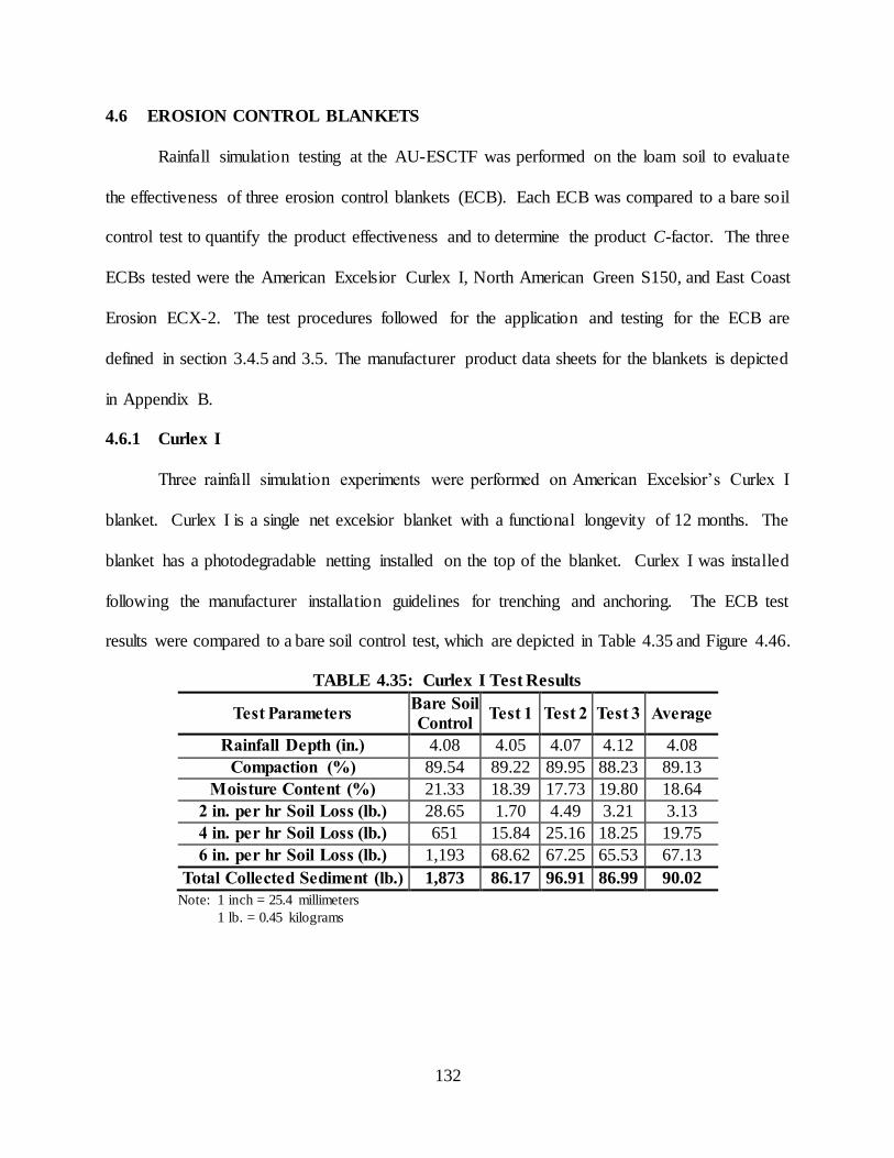
132
4.6 EROSION CONTROL BLANKETS
Rainfall simulation testing at the AU-ESCTF was performed on the loam soil to evaluate
the effectiveness of three erosion control blankets (ECB). Each ECB was compared to a bare soil
control test to quantify the product effectiveness and to determine the product C-factor. The three
ECBs tested were the American Excelsior Curlex I, North American Green S150, and East Coast
Erosion ECX-2. The test procedures followed for the application and testing for the ECB are
defined in section 3.4.5 and 3.5. The manufacturer product data sheets for the blankets is depicted
in Appendix B.
4.6.1 Curlex I
Three rainfall simulation experiments were performed on American Excelsior’s Curlex I
blanket. Curlex I is a single net excelsior blanket with a functional longevity of 12 months. The
blanket has a photodegradable netting installed on the top of the blanket. Curlex I was installed
following the manufacturer installation guidelines for trenching and anchoring. The ECB test
results were compared to a bare soil control test, which are depicted in Table 4.35 and Figure 4.46.
TABLE 4.35: Curlex I Test Results
Test Parameters Bare Soil
Control Test 1 Test 2 Test 3 Average
Rainfall Depth (in.) 4.08 4.05 4.07 4.12 4.08
Compaction (%) 89.54 89.22 89.95 88.23 89.13
Moisture Content (%) 21.33 18.39 17.73 19.80 18.64
2 in. per hr Soil Loss (lb.) 28.65 1.70 4.49 3.21 3.13
4 in. per hr Soil Loss (lb.) 651 15.84 25.16 18.25 19.75
6 in. per hr Soil Loss (lb.) 1,193 68.62 67.25 65.53 67.13
Total Collected Sediment (lb.) 1,873 86.17 96.91 86.99 90.02
Note: 1 inch = 25.4 millimeters
1 lb. = 0.45 kilograms

133
(a) Turbidity (b) TSS
FIGURE 4.46: Curlex I Water Quality Results.
The three Curlex I blanket experiments resulted in an average rainfall depth of 4.08 in.
(104 mm), an average slope compaction rate of 89.13%, and average moisture content of 18.64%.
The bare soil control test paired with the Curlex I blanket had a soil loss of 28.65 lb. (13 kg) during
the 2 in. per hr (51 mm per hr) rainfall intensity while the excelsior blanket only allowed an average
of 3.13 lb. (1.42 kg) of soil loss. The total soil loss for the bare soil control test was 1,873 lb.
(849.6 kg) while the Curlex I blanket had an average total soil loss of 90 lb. (40.8 kg). Therefore,
the blanket resulted in a 95% reduction in soil loss. Similar to the soil loss data, the turbidity and
TSS results were significantly less than the bare soil control test. The turbidity and TSS
measurements had an initial flush, but then leveled out for the remainder of the experiment even
though the rainfall intensity increased. The Curlex I blanket test performance is depicted in Figure
4.47.
0
20,000
40,000
60,000
80,000
100,000
120,000
140,000
0 20 40 60
Tu
rbid
ity
(NT
U)
Time (min)
Bare Soil Curlex I
0
50,000
100,000
150,000
200,000
0 20 40 60
TS
S (
mg
/L)
Time (min)
Bare Soil Curlex I

134
(a) Pre-test (b) 20 minute
(c) 40 minute (d) Post-test
FIGURE 4.47: Curlex I Test Photos.
4.6.1.1 Curlex I C-factor
Following the completion of the three Curlex I product experiments and a bare soil control
test, the rainfall depth and soil loss data from each experiment was used to calculate the product
C-factor. The bare soil control experiment was used to calculate the K-factor associated with the
three product experiments. The K-factor was calculated by plotting the soil loss in tons/acre vs.
the R-factor for the 2, 4, and 6 in. per hr (51, 102, 152 mm per hr) rainfall intensities as depicted
in Figure 4.48.

135
FIGURE 4.48: Curlex I K-factor Equation.
The linear equation from the trend line was used to calculate the corresponding A-factor
with the theoretical R-factor of 182.02. The corresponding A-factor was 119.45 tons per acre
(267.8 t/ha). The calculated A-factor was used in the RUSLE equation to calculate the soil
erodibility factor (K-factor). The resulting K-factor for the Curlex I experiment was 0.23.
Once the K-factor was calculated, the C-factor for the Curlex I blanket was determined
using two separate methods. The first method plotted the incremental C-factor vs. the incrementa l
R-factor for the three blanket experiments. The data for all three-rainfall intensities was used in
the graph because the means for all three rainfall intensity C-factors was equal the statistica l
analysis in section 4.6.1.2. The C-factor plot is depicted in Figure 4.49.
y = 0.6716x - 2.7923
R² = 0.9894
0
20
40
60
80
100
120
140
0 40 80 120 160 200 240
A(t
on/a
c)
R-factor

136
(a) Full test C-factor (b) Without 2 in. per hr C-factor
FIGURE 4.49: Curlex I C-factor Equation.
The 2, 4, and 6 in. per hr (51, 102, and 152 mm per hr) C-factors were statistically similar
means. Therefore, the linear trend line equation from Figure 4.49(a) was used to calculate the C-
factor corresponding with the theoretical R-factor of 182.02. The resulting C-factor for this
method was 0.049. The second method used to calculate the C-factor used the average A-factor
for each of the three product experiments was the RUSLE equation. The variables used to calculate
the C-factor are depicted in Table 4.36.
TABLE 4.36: Curlex I RUSLE Equation
A = 6.13
Theoretical R = 182.02
LS = 2.86
K = 0.23
P = 1.0
C = 0.0501
The resulting C-factor using the RUSLE equation was 0.050. Therefore, the two separate
calculation methods resulted in C-factor of 0.049 and 0.050.
4.6.1.2 Curlex I Statistical Analysis
Three hypothesis tests were performed on the incremental C-factors for the three Curlex I
blanket experiments. The three hypothesis tests compared the 2 to 4 in. per hr (51 to 102 mm per
y = 0.0001x + 0.0255
0.0
0.2
0.4
0.6
0.8
1.0
0 50 100 150 200
C-f
acto
r
R -factor
y = 9E-05x + 0.0313
0.0
0.2
0.4
0.6
0.8
1.0
0 50 100 150 200
C-f
acto
r
R-factor

137
hr), 2 to 6 in. per hr (51 to 152 mm per hr), and 4 to 6 in. per hr (102 to 152 mm per hr) C-factor
results to determine if the means of the resulting C-factors were equal. A hypothesis test was
performed on the incremental C-factors of the three S150 blankets evaluated under rainfa ll
simulation. If the two-tail p-value is less than the alpha value of 0.05 then the null hypothesis was
rejected and the means are not equal. The results from the three hypothesis tests are summarized
in Table 4.37.
TABLE 4.37: Curlex I Hypothesis Test Results
Hypothesis
Test
Intensity 1
Mean
Intensity 2
Mean p (two-tail)
2-4 in. per hr 0.0246 0.0371 0.228
2-6 in. per hr 0.0246 0.0488 0.074
4-6 in. per hr 0.0371 0.0488 0.197
The three hypothesis tests all resulted in p-values greater than the alpha value of 0.05.
Therefore, the means for all three combinations were equal and the null hypothesis was not
rejected.
4.6.2 S150
Three rainfall simulation tests were performed on North American Greens S150 ECB. The
S150 blanket is a double net straw fiber blanket with a functional longevity of 12 months. The
netting is a lightweight photodegradable netting located on the top and bottom of the blanket. The
S150 product specifications are depicted in Appendix B. The ECB was installed following the
manufacturers installation recommendations for trenching and anchoring. The S150 average water
quality measurements and soil loss results were compared to the performance of a bare soil control
test which is depicted in Table 4.38 and Figure 4.50.

138
TABLE 4.38: S150 Test Results
Test Parameters Bare Soil
Control Test 1 Test 2 Test 3 Average
Rainfall Depth (in.) 4.05 4.02 4.10 4.08 4.07
Compaction (%) 87.26 88.98 89.49 86.68 88.38
Moisture Content (%) 19.61 18.86 17.09 18.66 18.20
2 in. per hr Soil Loss (lb.) 97.58 13.59 2.77 5.55 7.30
4 in. per hr Soil Loss (lb.) 752 60.89 51.80 86.84 66.51
6 in. per hr Soil Loss (lb.) 1,245 230 223 200 218
Total Collected Sediment (lb.) 2,094 304 278 293 292
Note: 1 inch = 25.4 millimeters
1 lb. = 0.45 kilograms
(a) Turbidity (b) TSS
FIGURE 4.50: S150 Water Quality Results.
The three rainfall experiments performed on the S150 ECB resulted with an average
rainfall depth of 4.07 in. (103 mm), percent compaction of 88.38%, and an average moisture
content of 18.20%. The S150 blanket resulted in an average total soil loss of 292 lb. (132 kg).
The blanket resulted in an average soil loss of 7.30 lb. (3.3 kg) during the 2 in. per hr (51 mm per
hr) rainfall intensity and 66.5 lb. (30.2 kg) during the 4 in. per hr (102 mm per hr) rainfall intens ity.
However, the 6 in. per hr (152 mm per hr) rainfall intensity resulted in a higher soil loss of 218 lb.
(98.9 kg). The S115 ECB resulted in lower turbidity and TSS values than the corresponding bare
soil control test. The water quality measurements quickly increased to around 20,000 NTU during
0
20,000
40,000
60,000
80,000
100,000
120,000
140,000
0 20 40 60
Tu
rbid
ity
(NT
U)
Time (min)
Bare Soil Curlex I
0
50,000
100,000
150,000
200,000
0 20 40 60
TS
S (
mg/L
)
Time (min)
Bare Soil Curlex I

139
the 2 in. per hr (51 mm per hr) rainfall period and gradually increased for the remainder of the
experiment. The performance of the S150 ECB is depicted in Figure 4.51.
(a) Pre-test (b) 20 minute
(c) 40 minute (d) Post-test
FIGURE 4.51: S150 Test Photos.
4.6.2.1 S150 C-factor
Following the completion of the three S150 blanket experiments and a bare soil control
test, the rainfall depth, and soil loss data from each experiment was used to calculate the product
C-factor. The bare soil control resulted were used to calculate a K-factor for the three S150
experiments. The K-factor was calculated by plotting the soil loss in tons/acre versus the R-factor
for the 2, 4, and 6 in. per hr (51, 102, and 152 mm per hr) rainfall intensities as depicted in Figure
4.52.

140
FIGURE 4.52: S150 K-factor Equation.
The linear trendline equation was used to calculate the corresponding A-factor with the
theoretical R-factor of 182.02. The A-factor resulting from the calculation was 142.68 tons per
acre (63.64 t/ha). The calculated A-factor was used in the RUSLE equation to calculate the K-
factor. The resulting K-factor for the S150 experiment is 0.27.
Once the K-factor was calculated, the C-factor for the S150 blanket was determined using
two separate methods. The first method plotted the incremental C-factor versus the incrementa l
R-factor the three blanket experiments. Since the means for all three hypothesis tests were equal
in section 4.6.2.2, the 2, 4, and 6 in. per hr (51, 102, and 152 mm per hr) rainfall data was used in
the C-factor graph which is depicted in Figure 4.53.
y = 0.7631x + 3.7775R² = 0.9817
0
20
40
60
80
100
120
140
160
0 20 40 60 80 100 120 140 160 180 200
A(t
on/a
c)
R-factor

141
(a) Full test C-factor (b) Without 2 in. per hr C-factor
FIGURE 4.53: S150 C-factor Equation.
The 2, 4, and 6 in. per hr (51, 102, and 152 mm per hr) C-factors had statistically equal
means. Therefore, the linear trendline equation to calculate the C-factor corresponding with the
theoretical R-factor of 182.02. The calculated C-factor for this method was 0.144. The second
method used to calculate the C-factor used the average A-factor for each of the three S150
experiments with the RUSLE equation. The variables used to calculate the C-factor are depicted
in Table 4.39.
TABLE 4.39: S150 RUSLE Equation
A = 19.84
Theoretical R = 182.02
LS= 2.86
K = 0.27
P = 1.0
C = 0.143
The C-factor calculated using the average A-factor for each product experiment in the
RUSLE equation was 0.143. Therefore, the two separate methods calculated a C-factors of 0.144
and 0.143.
y = 0.0005x + 0.0578
0.0
0.2
0.4
0.6
0.8
1.0
0 50 100 150 200
C-
facto
r
R-factor
y = 0.0003x + 0.0891
0.0
0.2
0.4
0.6
0.8
1.0
0 50 100 150 200
C-f
acto
r
R-factor

142
4.6.2.2 S150 Statistical Analysis
Three hypothesis tests were performed on the incremental C-factors for the three S150
blanket experiments. The three hypothesis tests compared the 2-4 in. per hr (51-102 mm per hr),
2-6 in. per hr (51-152 mm per hr), and 4-6 in. per hr (102-152 mm per hr) C-factor results to
determine if the means of the resulting C-factors were equal. If the two-tail p-value is less than
the alpha value of 0.05 then the null hypothesis was rejected and the means are not equal. The
results from the three hypothesis tests are summarized in Table 4.40.
TABLE 4.40: S150 Hypothesis Test Results
Hypothesis
Test
Intensity 1
Mean
Intensity 2
Mean
Degrees of
Freedom P (two-tail)
2-4 in/hr 0.0502 0.1060 3 0.1381
2-6 in/hr 0.0502 0.1402 3 0.0650
4-6 in/hr 0.1060 0.1402 3 0.1179
The hypothesis tests resulted in a p-value greater than the alpha value of 0.05. Therefore,
the null hypothesis that the means are equal was true for all three experiments.
4.6.3 ECX-2
Three rainfall simulation experiments were performed on the East Coast Erosion’s ECX-2
(ECX-2) blanket. ECX-2 is a double net excelsior blanket with a functional longevity of 24
months. The netting is a photodegradable polypropylene netting installed on the top and bottom
of the excelsior fiber. The blanket was installed following the manufacturers recommendations
for trenching and anchoring. The blanket soil loss and water quality results were compared to a
bare soil control test which is depicted in Table 4.41 and Figure 4.54.

143
TABLE 4.41: ECX-2 Test Results
Test Parameters Bare Soil
Control Test 1 Test 2 Test 3 Average
Rainfall Depth (in.) 4.08 4.10 3.97 3.98 4.02
Compaction (%) 90.20 89.73 90.46 88.79 89.66
Moisture Content (%) 19.99 18.72 19.51 21.28 19.84
2 in. per hr Soil Loss (lb.) 104.70 0.98 3.23 5.08 3.10
4 in. per hr Soil Loss (lb.) 676.52 63.64 50.93 55.82 56.80
6 in. per hr Soil Loss (lb.) 1,174 202.43 121.31 159.55 161.10
Total Collected Sediment (lb.) 1,955 267 205 221 231
Note: 1 inch = 25.4 millimeters
1 pound = 0.45 kilograms
(a) Turbidity (b) TSS
FIGURE 4.54: ECX-2 Water Quality Results.
ECX-2 had an average total soil loss of 231 lb. (105 kg), rainfall depth of 4.02 in. (102
mm), and 89.66% compaction. The bare soil control test paired with the ECX-2 blanket had a
total soil loss of 1,955 lb. (886.8 kg), which means the blanket resulted in an 88% reduction in soil
loss. The blanket resulted in a low initial soil loss during the 2 in. per hr (51 mm per hr) rainfa ll
intensity and gradually increased as the rainfall intensity increased to 4 and 6 in. per hr (102 and
152 mm per hr). The turbidity measurements resulted in a high initial flush, but slowly reduced
for the remainder of the 2 in. per hr (51 mm per hr) rainfall intensity. Similar to the soil loss data,
the turbidity and TSS values gradually increased as the rainfall intensities increased. The excelsior
blankets test performance throughout the rainfall experiment is depicted in Figure 4.55.
0
20,000
40,000
60,000
80,000
100,000
120,000
140,000
0 20 40 60
Tu
rbid
ity
(NT
U)
Time (min)
ECX-2 Bare Soil
0
50,000
100,000
150,000
200,000
0 20 40 60
TS
S (
mg
/L)
Time (min)
ECX-2 Bare Soil

144
(a) Pre-test (b) 20 minute
(c) 40 minute (d) Post-test
FIGURE 4.55: ECX-2 Test Photos.
ECX-2 significantly reduced the water quality and soil loss results. However, there were
some areas in the installed blankets that were not filled with excelsior fiber, which did not provide
a protective cover for that area of the slope. Due to the lack of coverage, there was increased
erosion in those areas causing higher values of water quality and soil loss. The lack of excelsior
cover is depicted in Figure 4.56(a).
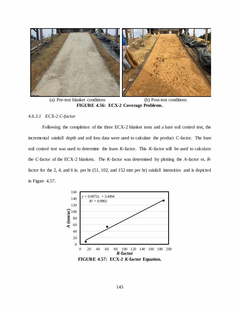
145
(a) Pre-test blanket conditions (b) Post-test conditions
FIGURE 4.56: ECX-2 Coverage Problems.
4.6.3.1 ECX-2 C-factor
Following the completion of the three ECX-2 blanket tests and a bare soil control test, the
incremental rainfall depth and soil loss data were used to calculate the product C-factor. The bare
soil control test was used to determine the loam K-factor. This K-factor will be used to calculate
the C-factor of the ECX-2 blankets. The K-factor was determined by plotting the A-factor vs. R-
factor for the 2, 4, and 6 in. per hr (51, 102, and 152 mm per hr) rainfall intensities and is depicted
in Figure 4.57.
FIGURE 4.57: ECX-2 K-factor Equation.
y = 0.6972x + 3.4494
R² = 0.9902
0
20
40
60
80
100
120
140
160
0 20 40 60 80 100 120 140 160 180 200
A(t
on
/ac)
R-factor

146
A linear trendline was used to determine a linear equation that best fits the data points. The
trendline equation was used to calculate the A-factor that corresponds with the theoretical R-factor
of 182.02. The A-factor calculated by this equation was 130.35 tons per acre (292.2 t/ha). This A-
factor was used in the RUSLE equation along with a LS-factor of 2.86, C-factor of 1.0, and P-
factor of 1.0. The resulting K-factor for this test group was 0.24.
Following the K-factor calculation, the C-factor for ECX-2 was determine following two
different methods. The first method plotted the incremental C-factor vs. the incremental R-factor
for the three ECX-2 experiments, which is depicted in Figure 4.57. The statistical analysis
performed in section 4.6.3.2 determined that the 2 in. per hr (51 mm per hr) C-factor mean was
not equal to the 4 or 6 in. per hr (102 or 152 mm per hr) means. Therefore, the 2 in. per hr (51 mm
per hr) data point was not used in this method because the resulting trend line was skewed due to
the small amount of erosion resulting in an inaccurate C-factor.
(a) Full test C-factor (b) Without 2 in. per hr C-factor
FIGURE 4.58: ECX-2 C-factor Equation.
The 2 in. per hr (51 mm per hr) C-factor mean was statistically different from the 4 and 6
in. per hr (102 and 152 mm per hr) C-factor means. Therefore, the linear trend line from Figure
4.58(b) was used to best fit the incremental data points. The C-factor was determined by solving
y = 0.0005x + 0.0383
0.0
0.2
0.4
0.6
0.8
1.0
0 50 100 150 200
C-f
acto
r
R-factor
y = 0.0002x + 0.0847
0.0
0.2
0.4
0.6
0.8
1.0
0 50 100 150 200
C-f
acto
r
R-factor

147
the linear equation for the theoretical R-factor of 182.02. The C-factor calculated for the ECX-2
using the first method was 0.121.
The second method used to calculate the ECX-2 C-factor plotted the incremental A-factor
versus the incremental R-factor for each of the three product experiments. A linear trendline was
used to calculate the A-factor that corresponds with the theoretical R-factor. All three of the A-
factors were averaged together to get the A-factor of 15.71 tons per acre (32.2 t per ha) for the
ECX-2 blanket. The data used to calculate the product C-factor is depicted in Table 4.42.
TABLE 4.42: ECX-2 RUSLE Equation
A = 15.71
Theoretical R = 182.02
LS = 2.86
K = 0.24
P = 1.0
C = 0.1238
The C-factor calculated using the RUSLE equation was 0.124. The first and second
methods used to calculate the C-factor resulted in values of 0.121 and 0.124 for the ECX-2
blankets.
4.6.3.2 ECX-2 Statistical Analysis
Three hypothesis tests were performed on the incremental C-factor calculated for the three
ECX-2 blanket experiments. The three hypothesis tests compared the 2 to 4 in. per hr (51 to 102
mm per hr), 2 to 6 in. per hr (51 to 152 mm per hr), and 4 to 6 in. per hr (102 to 152 mm per hr)
C-factor results to determine if the means of the resulting C-factors were equal. If the two-tail p-
value was less than the alpha value of 0.05 then the null hypothesis was rejected, concluding that
the means are not equal. The results from the three hypothesis tests for the ECX-2 blanket are
summarized in Table 4.43.

148
TABLE 4.43: ECX-2 Hypothesis Testing Results
Hypothesis
Test
Intensity 1
Mean
Intensity 2
Mean Alpha p (two-tail)
2-4 in. per hr 0.0242 0.0979 0.05 0.017
2-6 in. per hr 0.0242 0.1238 0.05 0.001
4-6 in. per hr 0.0979 0.1238 0.05 0.093
The three hypothesis tests performed on the ECX-2 blanket had varying results. The 2 to
4 in. per hr (51 to 102 mm per hr) and 2 to 6 in. per hr (51 to 152 mm per hr) hypothesis tests
resulted in p-values less than the alpha value of 0.05. Therefore, the null hypothesis was rejected,
concluding that the means are not equal. The 4 to 6 in. per hr (102 to 152 mm per hr) hypothesis
test resulted in a p-value greater than 0.05, concluding that the null hypothesis is true and that the
means are equal.
4.6.4 Erosion Control Blankets Summary
Three erosion control blankets were evaluated under large-scale rainfall simula t ion
consisting of American Excelsior’s Curlex I, North American Green’s S150, and East Coast
Erosion’s ECX-2. Three initial product performance tests were completed for each product and
each product was paired with a bare soil control test. The average soil loss results for the products
are depicted in Table 4.44.
TABLE 4.44: Erosion Control Blanket Soil Loss Summary
Product Soil Loss (lb.)
Bare Soil 1,974
Curlex I 90
S150 292
ECX-2 231 Note: 1 lb. = 0.45 kilograms
Curlex I resulted in the lowest total soil loss of 90 lb. (40.8 kg), which was 141 lb. (64 kg)
less than the second best blanket. The S150 blanket was the worst performing blanket with an
average soil loss of 292 lb. (132.4 kg). The average turbidity measurements for each product is
depicted in Figure 4.59.

149
FIGURE 4.59: ECB Turbidity Results.
All three of the blankets had an initial flush, but were followed by different results for the
remainder of the experiment. ECX-2 had the highest initial flush of 50,000 NTU and resulted in
the highest turbidity measurements throughout the remainder of the experiment. Curlex I had an
initial flush of only 18,000 NTU and then stabilized at roughly 10,000 NTU for the remainder of
the experiment. The rainfall depth and soil loss data for each blanket was used to calculate the
product C-factor. The C-factor was calculated using the regression and the RUSLE method, which
is depicted in Table 4.45.
TABLE 4.45: ECB C-factor Results
Product K-factor Regression Method RUSLE Method
Curlex I 0.23 0.049 0.050
S150 0.27 0.144 0.143
ECX-2 0.24 0.121 0.124
All three ECBs resulted in lower C-factors than the hydraulic mulches. Curlex I, which
had the lowest soil loss results, had the lowest C-factor of 0.05. S150, which had the highest
average soil loss, had the highest C-factor of 0.14. The S150 and ECX-2 blankets both had bare
spots within the blanket where there was minimal to no product. The lack of soil coverage in these
0
20,000
40,000
60,000
80,000
100,000
120,000
140,000
0 10 20 30 40 50 60
Turb
idit
y
(NT
U)
Time (min)
Bare Soil Curlex I S150 ECX-2

150
areas resulted in higher amounts of erosion. The Curlex I blanket did not have any bare spots
resulting in a better product performance than the other two blankets. If the bare spots in the ECX-
2 and S150 blankets were filled, the blanket performance would likely increase resulting in lower
C-factors.
4.6.5 Summary
In this study, erosion control practice performance was evaluated by the AU-ESCTF
rainfall simulator, which is designed to follow the ASTM D6459-19 rainfall event. Three init ia l
product performance tests were completed on each erosion control practice and compared to bare
soil control results. The soil loss ratio (SLR) was calculated for the straw mulch practices under
initial and longevity testing on the sandy loam soil. The erosion control product C-factor was
calculated on the loam soil for the products initial performance. The average soil loss from init ia l
product testing and the straw mulch longevity testing is summarized in Table 4.46.
TABLE 4.46: Rainfall Simulation Average Soil Loss Summary
Soil Type Erosion Control Practice
Average
Initial Soil
Loss (lb.)
SLR or
C-factor
Longevity
Soil Loss
(lb.)
Longevity
SLR
Sandy
Loam
Bare Soil 738 - 611 -
Loose Straw 143 0.19 287 0.47
Loose Straw with Tacking Agent 3
97 0.13 131 0.21
Crimped Straw 169 0.23 82 0.13
Loam
Bare Soil 2,154 - - -
Eco-Fibre plus Tackifier 1,038 0.55 - -
Soil Cover Wood Fiber plus Tack
1,164 0.46 - -
Terra-Wood with Tacking Agent 3
1,294 0.53 - -
Curlex I 90 0.05 - -
S150 292 0.14 - -
ECX-2 231 0.12 - -

151
The top performing erosion control practice tested in this study was American Excelsio r’s
Curlex I, which had a product C-factor of 0.05. The erosion control blankets were on average the
best performing erosion control practice tested for initial product performance. However, the loose
straw with Tacking Agent 3 evaluated on the sandy loam soil resulted in a SLR of 0.13, which is
comparable to North American Green’s S150 blanket with a C-factor of 0.14 and East Coast
Erosion’s ECX-2 blanket with a C-factor of 0.12. Longevity testing was only performed on the
sandy loam soil. For the initial product performance test, the crimped straw was the worst
performing straw mulch practice with a SLR of 0.23. However, when the crimped straw was
evaluated under longevity testing, the crimped straw had a SLR of 0.13, which is comparable to
the performance of two of the erosion control blankets. Three thermally processed wood with
tackifier hydraulic mulches were evaluated in this project. The hydraulic mulches experienced
high amounts of soil loss with a minimal C-factor of 0.46.

152
CHAPTER 5: CONCLUSION
5 CHAPTER 5: CONCLUSION
5.1 INTRODUCTION
The purpose of this research study was to re-design the existing rainfall simulator at the
AU-ESCTF to follow the ASTM D6459-19 (ASTM 2019) testing standards. A literature review
was performed to aid in the design of the rainfall simulator, the installation of erosion control
practices, and the rainfall simulator testing procedure. The rainfall simulator was calibrated for
rainfall intensity, uniformity, and drop size distribution. Following the calibration testing, rainfa ll
simulation testing was performed on bare soil and erosion control practices.
The first aspect of this research was to calibrate the rainfall simulator to produce 2, 4, and
6 in. per hr (51, 102, and 152 mm per hr) rainfall intensities. The existing rainfall simulator was
designed to produce the Alabama 2-yr, 24-hour storm event. There were six rainfall risers that
each had four sprinklers. The re-design of the rainfall simulator consisted of altering the
configuration of each riser to have three sprinklers each and to add four additional risers
surrounding the test plot to maximize rainfall uniformity. The optimal riser locations were
determined during the calibration testing. A calibration test consisted of a 15-minute rainfall event
for each rainfall intensity to determine the intensity and uniformity of the rainfall simulator. Once
the required rainfall intensity and uniformity were met, the drop size distribution was determined
using the flour pan method. Following the calibration testing, test plot preparation, testing, and
data collection procedures were developed. Rainfall simulation testing was performed to evaluate
the performance of erosion control practices as compared to bare soil conditions.

153
5.2 CALIBRATION TESTING
The rainfall simulator was designed to generate theoretical rainfall intensities of 2, 4, and
6 in. per hr (51, 102, and 152 mm per hr). Thirty, 15 minute calibration tests were conducted on
the rainfall simulator with 20 rain gauges installed on the test plot. Following each 15 minute
calibration test, rainfall depths were recorded for each rain gauge and used to calculate the rainfa ll
intensity and uniformity of the rainfall simulator. Ten calibration tests were conducted on each
rainfall intensity. A 5% difference from the theoretical rainfall depth was allowed for the
experimental rainfall depth. The uniformity of the rainfall was calculated using the Christiansen
Uniformity Coefficient with a minimum uniformity of 80% was required for each rainfall intens ity.
The experimental rainfall intensities resulting from calibration testing was 2.08, 4.12, and 6.07 in.
per hour (53, 105, 154 mm per hr). An ANOVA test was performed on each of the three rainfa ll
intensity calibration results to determine if the means between each of the calibration tests resulted
in equal means. The statistical analysis concluded that the calibration tests resulted in equal means
for the ten tests performed on the 2, 4, and 6 in. per hr (51, 102, and 152 mm per hr) rainfa ll
intensities. The uniformity coefficient calculated for each rainfall intensity ranged between 85.5-
87.5%. Since the rainfall depth and uniformity met the testing requirements, the drop size
distribution of the rainfall simulator was determined using the flour pan method. Three flour pan
tests were conducted for each rainfall intensity to accurately represent the drop sizes for the entire
test plot. The drop size distribution is depicted in Figure 4.1.
5.3 SANDY LOAM TESTING
Rainfall simulation testing was first performed on the sandy loam soil. Prior to the start of
rainfall simulation testing, a test plot preparation procedure was created to reach the desired
compaction rate of 86±6% and a moisture content within 5% of the testing soils optimum moisture

154
content. A test and data collection procedure were created to collect water samples for TSS and
turbidity measurements, total soil loss, rainfall depth, and discharge over time. Once these
procedures were completed, four bare soil control tests were conducted to determine the water
quality results throughout the experiment and the total soil loss of the experiment. The average
soil loss for the bare soil control test was 738 lb. (335 kg).
Following the bare soil control tests, three straw mulch applications were evaluated
including loose straw, loose straw with Tacking Agent 3, and crimped straw. The straw mulch
was installed at an application rate of two tons per acre for all three straw mulch applications. The
Tacking Agent 3 was sprayed on the loose straw at an application rate of 50 lb. per acre (56 kg per
ha). The straw was crimped a minimum of two inches into the soil in the perpendicular direction
to flow per the Alabama Handbook requirements. The rows of crimped straw were spaced a
maximum of eight inches with ¼ inch flat edged coulter blades. The straw applications had an
average total soil loss of 143 lb. (65 kg) for loose straw, 97 lb. (44 kg) for loose straw with Tacking
Agent 3, and 168 lb. (76 kg) for crimped straw. An ANOVA test was performed on the straw
mulch test results to determine if the soil loss between the three applications were equal. The
statistical analysis concluded that at least one of the means was not equal to the others. In order
to determine which means were equal, three hypothesis tests were performed to compare the loose
versus tackifier, loose versus crimped, and tackifier versus crimped straw applications. The
statistical analysis concluded that the loose straw and crimped straw had equal means and the straw
with tackifier was not equal to the crimped or loose straw applications. Under initial performance
testing, the loose straw with Tacking Agent 3 had the lowest water quality measurements and
lowest total soil loss. The tackifier was highly effective at the beginning of the experiment, but
the effect wore off over time. The crimped straw application had the highest soil loss and the worst

155
resulting water quality measurements. The poor performance by the crimped straw was due to the
disturbance of the soil as the straw was imbedded in the slopes surface.
Following the initial product testing for the straw mulch applications, a longevity test was
performed on each installation. The longevity tests had a total soil loss of 287 lb. (130 kg) for
loose straw, 131 lb. (59.4 kg) for loose straw with Tacking Agent 3, and 82 lb. (37.2 kg) for
crimped straw. The additional rainfall event resulted in significant improvement in the
effectiveness of the crimped straw. The crimped straw improved from having the highest soil loss
under initial product testing to having the lowest soil loss for longevity testing. The loose straw
resulted in the highest soil loss and water quality measurements under longevity testing. The
decrease of loose straw performance was due to the straw washing from the test plot, which
reduced the amount of soil cover. The loose straw with Tacking Agent 3 resulted in similar water
quality measurements as the crimped straw but had a higher total soil loss. The evaluation of the
three straw mulch applications on a 3H:1V slope proved that anchoring straw mulches provides
longer lasting coverage and reduces the amount of erosion.
5.4 LOAM SOIL TESTING
Following the straw mulch testing on the sandy loam soil, testing transitioned to a soil type
that better aligned to the ASTM D6459-19 soil requirements of a clay, loam, or sand. Therefore,
a soil analysis was performed on local soil stockpiles until a soil met the standard requirements.
Following the soil analysis, 12 in. (30.5 cm) of the sandy loam soil was excavated from the test
plot and replaced with 12 in. (30.5 cm) of loam soil. Once the test plot was reconstructed, rainfa ll
simulation testing was continued to evaluate the performance of bare soil, hydraulic mulches, and
erosion control blankets (ECB).

156
The testing procedure was performed differently for the loam soil experiments so that the
RUSLE C-factor could be calculated for each erosion control product. The rainfall simulator was
stopped between each 20 minute rainfall intensity interval to measure the rainfall depth and to
separate the soil loss into separate containers.
5.4.1 Hydraulic Mulches
Rainfall simulator testing was performed on three hydraulic mulches consisting of Eco-
Fibre plus Tackifier, Soil Cover Wood Fiber with Tack, and Terra-Wood with Tacking Agent 3.
All three of the hydraulic mulches were installed following the manufacturer recommendations at
an application rate of 2,500 lb. per acre (2,802 kg per ha). The hydraulic mulches were allowed
to cure for a minimum of 24 hours prior to rainfall simulation testing. The bare soil control
experiments paired with the hydraulic mulch products resulted in an average soil loss of 2,333 lb.
(1,058 kg). The total soil loss for the hydraulic mulches was 1,038 lb. (471 kg) for the Eco-Fiber,
1,164 lb. (528 kg) for the Soil Cover, and 1,294 lb. (587 kg) for the Terra-Wood. During the 2 in.
per hr (51 mm per hr) rainfall intensity the soil loss for each of the products was 3.45 lb. (1.56 kg)
for the Eco-Fiber, 2.67 lb. (1.21 kg) for the Soil Cover, and 8.54 lb. (3.87 kg) for the Terra-Wood.
The hydraulic mulch performed well during the 2 in. per hr (51 mm per hr) rainfall intens ity.
However, as the rainfall intensity increased to 4 in. per hr (102 mm per hr), the hydraulic mulches
experienced greater soil losses of 337 lb. (153 kg) for Eco-Fibre, 382 lb. (173 kg) for Soil Cover,
and 491 lb. (223 kg) for Terra-Wood. The increase in soil loss between the 2 and 4 in. per hr (51
and 102 mm per hr) rainfall intensities was caused by the mulch washing from the test plot. Once
the hydraulic mulch had washed from the test plot, there were large areas of exposed soil resulting
in substantial rill formation and high water quality measurements and soil loss.

157
Following the completion of the hydraulic mulch testing, a procedure for calculating the
product C-factor was created using the drop size distribution, incremental soil loss, and the
incremental rainfall depth for each experiment. Two separate procedures were used to calcula te
the product C-factors, which is referenced in section 3.7.2. Three hypothesis tests were performed
on the incremental soil loss results for each hydraulic mulch to determine if the C-factors between
the 2 to 4, 2 to 6, and 4 to 6 in. per hr (51 to 102, 51 to 152, and 102 to 152 mm per hr) rainfa ll
intensities had equal means. All three of the hydraulic mulches resulted in the 4 to 6 in. per hr
(102 to 152 mm per hr) rainfall intensities to have C-factors with equal means. The 2 to 4 and 2
to 6 in. per hr (51 to 102 and 51 to 152 mm per hr) rainfall intensities mean C-factors were not
equal. The results from this statistical analysis were used to calculate the product C-factor in the
regression method. The 2 in. per hr (51 mm per hr) C-factor was not included in the C-factor
versus R-factor graph because its mean was not equal to the 4 or 6 in. per hr (102 or 152 mm per
hr) C-factors. The resulting C-factors for the hydraulic mulches was 0.55 for Eco-Fibre, 0.46 for
Soil Cover, and 0.54 for Terra-Wood. The Soil Cover hydraulic mulch had the highest C-factor
of 0.46. The Eco-Fibre hydraulic mulch had a higher C-factor because one of the experiments was
exposed to excess rainfall from a storm that occurred prior to the collection of the 6 in. per hr (152
mm per hr) soil loss data. All three of the hydraulic mulches had relatively high C-factors. Other
erosion control practices should be used to reduce the amount of erosion occurring on the test plot.
5.4.2 Erosion Control Blankets
Three erosion control blankets were evaluated under rainfall simulation testing consisting
of American Excelsior’s Curlex I, North American Green’s S150, and East Coast Erosion’s ECX-
2. The installation of the ECBs followed manufacturer recommendations for trenching and
anchoring. The bare soil control experiments paired with the three ECBs resulted in an average

158
total soil loss of 1,974 lb. (895 kg). The total soil loss for the ECBs was 90 lb. (40.8 kg) for Curlex
I, 292 lb. (132 kg) for S150, and 231 lb. (105 kg) for ECX-2. All three of the blankets had an
increase in soil loss as the rainfall intensity increased. The 2 in. per hr soil loss for the ECBs was
3.13 lb. (1.42 kg) for Curlex I, 7.30 lb. (3.31 kg) for S150, and 3.10 lb. (1.41 kg) for ECX-2. The
ECBs soil loss during the 4 in. per hr (102 mm per hr) rainfall intensity was 19.75 pounds (8.95
kg) for Curlex I, 66.51 lb. (30.2 kg) for S150, and 56.8 lb. (25.7 kg) for ECX-2. All three blankets
had similar soil loss results during the 2 in. per hr (51 mm per hr) rainfall intensity. During the 4
and 6 in. per hr (102 and 152 mm per hr) rainfall intensities, the soil loss for the S150 and ECX-2
blankets increased at a higher rate than the 2 in. per hr (51 mm per hr) rainfall intensity. The S150
and ECX-2 blankets had bare spots where no blanket filler was located, resulting in little to no
cover for those areas. The lack of cover caused the erosive forces of the rainfall to increase the
amount of erosion occurring at those bare spots. If the S150 and ECX-2 blankets covered the test
plot like the Curlex I blanket, then the soil loss results would be reduced.
Following the completion of product testing, the C-factors for each ECB was calculated
using the incremental soil loss and the rainfall depth. The bare soil control results paired with each
ECB was used to calculate the K-factor associated with each blanket test. Three hypothesis tests
were performed on the incremental soil loss results for each ECB to determine if the C-factors
between the 2 to 4, 2 to 6, and 4 to 6 in. per hr (51 to 102, 51 to 152, and 102 to 152 mm per hr)
rainfall intensities had equal means. The Curlex I and S150 blankets resulted in equal C-factor
means for all three rainfall intensity combinations. Therefore, all three rainfall intensities C-factor
data was used in the regression method to aid in the product C-factor calculation. The ECX-2
blanket resulted in the 2 to 4 and 2 to 6 in. per hr (51 to 102 and 51 to 152 mm per hr) rainfa ll
intensities mean C-factors not being equal. The 2 in. per hr (51 mm per hr) C-factor data was not

159
included in the C-factor versus R-factor graph because its mean was not equal to the 4 or 6 in. per
hr (102 or 152 mm per hr) C-factors. The results from this statistical analysis were used to
calculate the product C-factor in the regression method. The C-factors calculated for each product
was 0.05 for Curlex I, 0.14 for S150, and 0.12 for ECX-2. If the S150 and ECX-2 blankets did
not have the bare spots with no filler, the product C-factors could have been closer to the Curlex I
C-factor.
All three of the blankets resulted in lower C-factors than the hydraulic mulches. The
hydraulic mulches washing from the test plot caused the difference in performance between the
hydraulic mulches and ECBs. The hydraulic mulches and ECBs resulted in similar soil loss results
for the 2 in. per hr (51 mm per hr) rainfall intensity. However, when the rainfall intensity increased
to 4 in. per hr (102 mm per hr), the hydraulic mulch would wash from the test plot causing a lack
of coverage while the blankets remained anchored in place for the full duration of the experiment.
5.5 SUMMARY
This research study had four primary objectives that were addressed throughout this
project. Based on the research performed in this study, the objectives were addressed as follows.
1. The AU-ESCTF rainfall simulator was redesigned from the existing rainfa ll
simulator to follow the ASTM D6459-19 design requirements. This rainfa ll
simulator was designed and calibrated to produce 2, 4, and 6 in. per hr (51, 102,
and 152 mm per hr) rainfall intensities. Ten calibration tests were performed on
each rainfall intensity to measure the experimental rainfall intensity and uniformity.
The experimental rainfall intensities resulting from calibration testing was 2.08,
4.12, and 6.07 in. per hour (53, 105, 154 mm per hr) and had rainfall uniformit ies
ranging from 85-87%. The drop size distribution of the rainfall simulator was

160
determined by using the flour pan method. The drop size distribution results are
summarized in section 4.2.2.
2. The test procedures used in this study followed the ASTM D6459-19 specificat ions
for test plot preparation and data collection. The test plot was tilled, raked, and
compacted with a turf roller in preparation for each rainfall experiment. The
compaction rate and moisture content of the test slope were evaluated through the
drive cylinder compaction test. Test procedures were created to collect water
samples at three-minute intervals, measure rainfall depth, collect soil loss, and
measure discharge over time. Following a rainfall experiment, procedures were
established for the measurement of total soil loss and the water sample results for
TSS and turbidity. Following the straw mulch testing, test procedures were updated
to allow for product C-factor calculations by separating each rainfall intensities soil
loss and measuring rainfall depth for each rainfall intensity.
3. This study evaluated erosion control practices listed on ALDOT’s preferred
products List II-11 and II-20. Throughout this project, three straw mulch
applications, hydraulic mulches, and erosion control blankets from ALDOT’s
preferred products lists were evaluated. The straw mulch practices evaluated in this
study were loose straw, loose straw with Tacking Agent 3, crimped straw. The
hydraulic mulches evaluated in this study were Profile Products Eco-Fibre plus
Tackifier, Profile Products Soil Cover Wood Fiber with Tack, and Profile Products
Terra-Wood with Tacking Agent 3. The three erosion control blankets tested in
this study were American Excelsior’s Curlex I, North American Green’s S150, and
East Coast Erosion’s ECX-2.

161
4. During this project, a procedure was developed to calculate the erosion control
practice C-factor using the RUSLE equation. The procedure uses the drop size
distribution data, incremental rainfall depth, and the incremental soil loss for each
experiment. A bare soil control test was paired with each erosion control practice
to calculate the soils K-factor, which was used for the product C-factor calculat ion.
The data collected from the three erosion control practice tests were used to
calculate the product C-factor. Two separate C-factor calculation procedures were
created during this project, which are compared in this study.
5.6 RECOMMENDATIONS FOR FURTURE RESEARCH
The research presented in this study shows that the AU-ESCTF rainfall simulator is capable
of consistently simulating the ASTM D6459-19 rainfall event. The test procedures and rainfa ll
simulation results found in this study should be used to pursue accreditation for ASTM D6459-19
testing through the Geosynthetic Accreditation Institute (GAI). As rainfall simulation testing
continues, additional erosion control practices should be tested to better understand product
performance on a 3H:1V slope. In this study, anchored straw mulch was evaluated on the sandy
loam soil. Future research should evaluate the performance of the same anchored straw
applications on the loam soil. Additional mulching applications (pine straw, peanut hulls, and
wood chips) should be tested to compare the performance of straw mulches with other mulching
practices. In this study, hydraulic mulches were only effective during the 2 in. per hr (51 mm per
hr) rainfall intensity and resulted in large amounts of erosion. Since the wood with tack hydraulic
mulches were ineffective under the ASTM D6459-19 rainfall event, future testing should evaluate
higher strength hydraulic erosion control products (HECPs) such as ProMatrix Engineered Fiber
Matrix and Flexterra Flexible Growth Medium. Profile Products representatives recommended

162
using the ProMatrix and Flexterra products for the ASTM D6459 testing parameters. ProMatrix
and Flexterra are designed to withstand higher shear stresses and flow velocities than ordinary
wood with tack hydraulic mulches. These two products use crimped biodegradable interlock ing
fibers and micro pore granules to increase the strength of the product. Unlike the wood with tack
hydraulic mulches tested in this study, the ProMatrix mulch is designed to withstand a 3H:1V slope
length of 50 ft (15.2 m) without slope interrupters while Flexterra is designed to withstand 100 ft
(30.5 m) slope length. The hydraulic mulches in this study were installed on a smooth slope, which
affected the performance of the products. Future testing should compare the hydraulic mulch
effectiveness with and without tracking. All three of the hydraulic mulches evaluated in this study
are designed for slopes less than 30 ft (9.1 m.) long. Future research should install slope
interrupters on the slope to evaluate the performance of the hydraulic mulches with and without
slope interrupters. ECBs were the most effective erosion control practice evaluated in this study.
Future research should be performed on ECBs with varying fillers such as straw, excelsior, straw/
coconut, and coconut and varying biodegradable netting options such as woven jute and coir
nettings. In addition to these ECBs, a polymer-enhance soft armoring system (PAM and jute),
which has been evaluated under small-scale rainfall simulation at the AU-ESCTF, should be tested
to compare this system to the small-scale results and the results of other erosion control practices
under large-scale rainfall simulation.
Based upon this research performed at the AU-ESCTF, the following recommendations
are made to better enhance future testing efforts.
1) Additional rainfall simulators should be constructed to increase the capabilities of the
test facility.

163
2) When constructing additional rainfall simulators, the design of the rainfall simula tor
should be altered from the original design to reduce the slope preparation, testing, and data
collection time. The test plots should be lined with concrete to prevent the erosion of the area
surrounding the rainfall simulator and to increase safety. The catch basin should not be wider than
the test plot to prevent runoff from areas other than the test plot from entering the catch basin. A
removable winch mounting system should be installed at the top of the test slope to allo w
equipment easy access to the top of the test plot. The ease of access for the equipment would
decreased the time it takes to rebuild the test plot. The electrical control box should be moved to
the bottom of the test plot for ease of access during an experiment and to allow the equipment
access at the top of the slope.
3) During this research project, a pulley system was installed on the wind curtains;
however, this system was not a viable long-term option. Future wind curtain systems that have an
efficient and effective pulley system would reduce the amount of time required to install the wind
curtains. During the construction of future wind curtains, ensure the wind curtains are able to be
installed to better mimic the slope of the plots so that better coverage is provided. The existing
rainfall simulators wind curtains have resulted in a system that at some points are shorter than the
sprinklers, causing some minimal wind disruption.

164
REFERENCES
Alabama Department of Transportation (2018).“Standard Specifications for Highway Construction.” Montgomery, AL.
Alabama Soil and Water Conservation Committee (2018).“Alabama Handbook for Erosion Control, Sediment Control and Stormwater Management on Construction Sites and Urban Areas.” Montgomery, AL.
ASTM (2008). “Standard Test Method for Determination of Water (Moisture) Content of Soil by Microwave Oven Heating.” West Conshohocken, PA, 1-7.
ASTM (2010). “Standard Test Method for Density of Soil in Place by the Drive-Cylinder Method.” West Conshohocken, PA, 1-7.
ASTM (2012). “Standard Test Method for Laboratory Compaction Characteristics of Soil Using
Standard Effort (12,400 ft-lbf/ft3 (600 kN-m/m3)).” West Conshohocken, PA, 1-13.
ASTM (2013). “Standard Test Methods for Filterable Matter (Total Dissolved Solids) and
Nonfilterable Matter (Total Suspended Solids) in Water.” West Conshohocken, PA, 1-9.
ASTM (2014). “Standard Test Method for Sieve Analysis of Fine and Coarse Aggregates.” West Conshohocken, PA, 1-5.
ASTM (2017). “Standard Test Method for Determina tion of Turbidity Above 1 Turbidity Unit (TU) in Static Mode.” West Conshohocken, PA, 1-22.
ASTM (2017). “Standard Test Method for Liquid Limit, Plastic Limit, and Plasticity Index of Soils.” West Conshohocken, PA, 1-20.
ASTM (2017). “Standard Test Method for Materials Finer than 75-µm (No. 200) Sieve in Mineral
Aggregates by Washing.” West Conshohocken, PA, 1-4.
ASTM (2017). “Standard Test Method for Particle-Size Distribution (Gradation) of Fine-Grained
Soils Using the Sedimentation (Hydrometer) Analysis.” West Conshohocken, PA, 1-25.
ASTM (2019). “Standard Test Method of Rolled Erosion Control Product (RECPs) Performance in Protecting Hillslopes from Rainfall Induced Erosion.” West Conshohocken, PA, 1-10.
Barnett, A. P., Diseker, E. G., and Richardson, E. C. (1967). “Evaluation of Mulching Methods for Erosion Control on Newly Prepared and Seeded High Backslopes.” Agronomy Journal,
Vol. 59, 83-85.
Benik, S. R., Wilson, B.N., Biesboer, D. D., Hansen, B., and Stenlund, D. (2003). “Performance
of Erosion Control Product s on a Highway Embankment.” Transactions of ASABE,
46(4), 1113-1119.

165
Bjorneberg, D. J., Aase, J. K., and Westermann, D. T. (2000). "Controlling Sprinkler Irrigation
Runoff, Erosion, and Phosporus Loss with Straw and Polyacrylamide." Soil and Water
Division of ASAE , 1545-1551.
Brady, N. C., and Weil, R. R. (1999). The Nature and Properties of Soils, Prentice Hall, Upper
Saddle River, New Jersey.
Bubenzer, G. D., and Jones Jr., B. A. (1971). “Drop Size and Impact Velocity Effects on the Detachment of Soils under Simulated Rainfall.” Transactions of the ASABE, 14(4), 625-628.
Cabalka, D. A., Clopper, P. E., Johnson, A. G., and Vielleux, M. T. (1998).“Research, Development and Implementation of Test Protocols for Rainfall Erosion Facilit ies (REFS).” American Excelsior Company – Earth Science Division.
Clopper, P. , Vielleux, M., and Johnson, A. (2004)."Quantifying the Performance of Hillslope
Erosion Control Best Management Practices." American Society of Civi Engineers, 1-10.
Early, J. J., Clopper, P. E., and Johnson, T. "Quantitative Erosion Control Product Testing Under
Simulated Rainfall.", 293-300.
ECTC (2014). "Rolled Erosion Control Products (RECPs) General Usage and Installa t ion
Guidelines for Slope. " https://www.ectc.org/rolled-erosion-control-products-recps-.
Eigel, J. D., and Moore, I. D. (1983). "A Simplified Technique for Measuring Raindrop Size and
Distribution." American Society of Agricutural Engineers Soil and Water Division, 1079-
1084.
Elbasit, M. A. M., Ojha, C. S. P., Ahmed, Z., Yasuda, H., Salmi, A., and Ahmed, F. (2015). “Rain Microstructure and Erosivity Relationships under Pressurized Rainfall Simulator.” Journal
of Hydrologic Engineering, 1-6.
Faucette, L.B., Governo, J., Jordan, C.F., Lockaby, B.G., Carino, H.F., and Governo, R. (2007).
"Erosion Control and Storm Water Quality from Straw with PAM, Mulch, and Compost
Blankets of Varying Particle Size." Soil and Water Conservation, 404-413.
Foltz, R.B., and Dooley, J.H. (2003). “Comparison of Erosion Reduction between Wood Strands
and Agricultural Straw.” American Society of Agricultural Engineers, 1389-1396.
Gholami, L., Sadeghi, S.H., and Homaee, M. (2012). "Straw Mulching Effect on Splash Erosion,
Runoff, and Sediment Yield from Eroded Plots." Soil Science Society of America, 268-
278.
Hall, M. J. (1970). "Use of the Stain Method in Determination the Drop-Size Distribution of
Coarse Liquid Sparys." American Society of Agricutural Engineers, 33-41.
Holt , G., Buser, M., Harmel, D., and Potter, K. (2005)."Comparison of Cotton-based Hydro-
mulches and Conventional Wood and Paper Hydro-mulches - Study II." Journal of
Cotton Science, 128-134.

166
Horne, M.A., Zech, W.C., Fang, X., and Vasconcelos, J.G. (2017). “Design and Construction of a Rainfall Simulator for Large Scale Testing of Erosion Control Practices and Products.”
Auburn University.
Jayawardena, A.W., and Rezaur, R.B. (2000). "Measuring Drop Size Distribution and Kinetic
Energy of Rainfall Using a Force Transducer." Hydrological Processes, 37-49.
Karpilo Jr., R. D., and Toy, T. J. (2004). “RUSLE C-Factors for Slope Protection Applications. ”
Journal American Society of Mining and Reclamation, vol. 2004, no. 1, 995–1013.
Kathiravelu, G., Lucke, T., and Nichols, P. (2016). "Rain Drop Measurement Techniques: A
Review." Water, 8(29), 1-20.
Khan, M. N., Gong, Y., Hu, T., Lal, R., Zheng, J., Justine, M. F., Azhar, M., Che, M., and Zhang, H. (2016). "Effect of Slope, Rainfall Intensity and Mulch on Erosion and Infiltration under
Simulated Rain on Purple Soil of Soiuth Western Sichuan Province, China." Water, 8 (528), 1-18.
Kincaid, D C, Solomon, K. H., and Oliphant, J. C. (1996). "Drop Size Distribution for Irrigation
Sprinklers." American Society of Agricultural Engineers, 839-845.
Laws, J. O., and Parsons, D. A. (1943). "The Relation of Raindrop-Size to Intensity." Transactions of the American Geophysical Union, 24, 452-460.
Lipscomb, C. M., Johnson, T., Nelson, R., and Lancaster, T. (2006). "Comparison of Erosion
Control Technologies: Blown Straw vs. Erosion Control Blankets." Erosion Control
Technology Council.
Mid-American Regional Council (2020). “What is Sediment Pollution ”
https://cfpub.epa.gov/npstbx/files/ksmo_sediment.pdf
Ming-Han, L. (2014). “Evaluating erosion control performance of crimped straw mulch in comparison with RECPs on simulated highway roadsides.” International Journal of
Geotechnical Engineering, 307-314.
Ming-Han, L., McFalls, J., and Yi, Y. (2013). "Comparing Erosion Control Products
Performance Results from Field and Large-Scale Laboratory Testing ." Indian
Geotechnical Society,: 382-387.
Novotny, V. (2003). Water Quality: Diffuse Pollution and Watershed Management , J. Wiley, Hoboken, New Jersey.
Pall, R., Dickinson, W. T., Beals, D., and McGirr, R. (1983). “Development and Calibration of a
Rainfall Simulator.” Canadian Agricultural Engineering, Vol. 25, 181-187.
Rickson, R J. (2006)."Controlling Sediment at Source: An Evaluation of Erosion Control Geotextiles." Wiley Interscience, 550-560.
Risse, M., and Faucette, B. (2001). “Compost Utilization for Erosion Control. University of
Georgia Cooperative Extension Service Bulletin 1200. Athens, GA.

167
Robeson, M. D., Abt, S. R., Watson, C. C., and Williams, J. D. (2014). “Unification of Large-Scale Laboratory Rainfall Erosion Testing.” Colorado State University.
U.S. Department of Agriculture, Agricultural Research Service. (1978). “Predicting Rainfa ll
Erosion Losses.” Agriculture Handbook No. 537, Washington, D.C.
U.S. Department of Agriculture, Agricultural Research Service. (1997). “Predicting Soil Erosion by Water: A Guide to Conservation Planning with the Revised Universal Soil Loss
Equation.” Agriculture Handbook No. 703, Washington D.C.
U.S. Environmental Protection Agency.(2019). “EPA's 2017 Construction General Permit (CGP) and Related Documents.” Retrieved fromhttps://www.epa.gov/npdes/epas-2017-
construction-general-permit-cgp-and-related-documents.
Wilson , W. T., Zech, W. C., Clement, P., Crowley, L. G. (2010) "Evaluation of Hydromulches
as an Erosion Control Measure Using Intermediate - Scale Experiments." Auburn
University.
Ziegler , A D, Sutherland, R. A., and Tran, L. T. (1997). "Influence of Rolled Erosion Control
Systems on Temporal Rainsplash Response - A Laboratoray Rainfall Simulation
Experiment ." Land Degredation and Development, 139-157.

168
APPENDICES
Appendix A: Manufacturer Specifications for Rainfall Simulator Components
Appendix B: Erosion Control Product Specifications
Appendix C: Experimental Data

169
APPENDIX A
MANUFACTURER SPECIFICATIONS FOR RAINFALL SIMULATOR COMPONENTS

170

171

172

173

174

175

176
APPENDIX B
EROSION CONTROL PRODUCT SPECIFICATIONS

177

178

179

180

181

182

183

184

185

186

187

188
APPENDIX C
EXPERIMENTAL DATA

189
TABLE C.1: 2 in./hr Rainfall Calibration Data
Rain
Gauge
Number
Test
1
Test
2
Test
3
Test
4
Test
5
Test
6
Test
7
Test
8
Test
9
Test
10
1 1.6 1.4 1.4 1.6 1.6 1.0 1.0 1.1 1.3 1.6
2 1.6 1.2 1.5 1.6 1.5 1.0 0.9 1.1 1.2 1.2
3 1.4 1.2 1.4 1.4 1.4 1.3 1.2 1.2 1.0 1.0
4 1.4 1.6 1.3 1.4 1.4 1.8 1.8 1.6 1.6 1.7
5 1.6 1.6 1.7 1.6 1.5 1.0 1.1 1.6 1.6 1.9
6 1.0 1.2 0.9 1.0 1.0 1.4 1.4 1.4 1.5 1.2
7 0.9 1.1 1.0 0.9 1.0 1.8 1.7 1.6 1.4 1.4
8 1.8 2.2 2.1 1.8 1.8 1.8 1.8 1.5 1.6 1.4
9 1.3 1.4 1.4 1.3 1.3 1.3 1.6 1.5 1.8 1.5
10 1.2 1.3 1.4 1.2 1.2 1.2 1.0 1.1 1.0 1.2
11 1.5 1.7 1.6 1.5 1.4 1.4 1.4 1.4 1.4 1.5
12 1.1 1.1 1.0 1.1 1.0 1.2 1.1 1.0 1.1 1.0
13 1.4 1.3 1.4 1.4 1.6 1.6 1.7 1.4 1.4 1.4
14 1.5 1.7 1.4 1.5 1.6 1.7 1.6 1.6 1.6 1.6
15 1.0 1.2 1.2 1.0 1.2 1.6 1.8 1.4 1.4 1.2
16 0.9 1.0 0.8 0.9 0.8 1.6 1.5 1.0 1.2 1.1
17 1.8 1.8 2.0 1.8 2.0 1.0 1.3 1.2 1.1 1.4
18 1.3 0.9 1.0 1.3 1.3 1.6 1.4 1.0 1.0 1.2
19 0.7 0.6 0.7 0.7 0.7 1.6 1.2 0.7 0.8 0.6
20 1.0 1.2 1.0 1.0 0.9 1.2 1.0 0.8 0.8 0.8
Results
Number of Observations 20 Total Rainfall Depth 26.4 cm
Avg. Rainfall Depth 1.32 cm
∑|Vi-VAvg| (cm) 3.78 cm
Coefficient of Uniformity (Cu) 85.67 %
Avg. Rainfall Intensity 5.272 cm/hr
Avg. Rainfall Intensity 2.08 in/hr
Standard Deviation 0.043

190
TABLE C.2: 4 in./hr Rainfall Calibration Data
Rain Gauge
Number
Test
1
Test
2
Test
3
Test
4
Test
5
Test
6
Test
7
Test
8
Test
9
Test
10
1 3.2 2.6 3.2 3.1 3.1 2.4 2.4 2.2 1.9 2.1
2 3.4 2.9 3.7 3.5 3.2 2.2 2.2 2.4 2.4 2.4
3 2.8 2.9 2.6 2.6 2.7 2.8 2.8 2.6 2.8 2.6
4 3.1 3.2 2.8 2.5 2.8 3.6 3.6 3.6 3.6 3.6
5 2.9 2.6 2.6 2.6 2.6 2.6 2.6 2.8 2.4 2.5
6 2.2 2.4 2.6 2.9 2.6 2.4 2.4 2.4 2.8 2.6
7 2.5 2.8 2.4 2.8 2.9 3.0 3.0 2.8 3.1 3.2
8 3.4 3.6 3.3 2.9 3.1 3.3 3.3 3.3 4.0 3.6
9 2.6 2.4 2.3 2.2 2.4 2.9 2.9 3.0 3.4 3.0
10 2.0 2.1 1.9 1.7 2.1 2.2 2.2 2.0 2.4 2.4
11 2.8 2.6 2.8 2.6 2.8 2.5 2.5 2.4 2.2 2.3
12 2.8 2.5 3.0 3.2 2.8 2.5 2.5 2.3 2.3 2.4
13 3.4 3.4 3.2 2.7 3.2 2.9 2.9 3.0 3.4 3.2
14 3.3 3.2 2.9 2.6 2.9 3.0 3.0 3.2 3.6 3.4
15 2.8 2.4 2.4 2.1 2.2 2.8 2.8 2.7 2.8 2.9
16 1.8 2.0 1.9 1.8 1.9 2.4 2.4 2.3 2.5 2.3
17 3.2 3.8 2.8 2.9 3.1 2.6 2.6 2.5 2.5 2.4
18 2.7 2.5 2.8 2.5 2.6 2.3 2.3 2.2 2.0 2.0
19 1.6 1.4 1.7 1.5 1.6 1.7 1.7 1.6 1.8 1.7
20 2.0 2.1 1.4 1.5 1.7 1.8 1.8 1.8 1.8 1.8
Results
Number of Observations 20 Total Rainfall Depth 52.4 cm
Avg. Rainfall Depth 2.62 cm
∑|Vi-VAvg| (cm) 6.55 cm
Coefficient of Uniformity (Cu) 87.49 %
Avg. Rainfall Intensity 10.47 cm/hr
Avg. Rainfall Intensity 4.12 in/hr
Standard Deviation 0.063

191
TABLE C.3: 6 in./hr Rainfall Calibration Data
Rain Gauge
Number
Test
1
Test
2
Test
3
Test
4
Test
5
Test
6
Test
7
Test
8
Test
9
Test
10
1 3.4 3.4 2.9 2.9 3.5 3.8 4.0 4.2 4.0 4.0
2 3.7 3.6 4.3 3.5 3.9 4.0 3.7 4.5 4.6 4.4
3 4.0 3.9 4.2 4.2 4.2 4.3 3.6 4.4 4.2 4.3
4 5.1 5.2 4.7 4.5 4.5 4.0 4.3 4.2 4.2 4.0
5 4.0 4.0 3.4 3.6 3.6 4.0 4.6 4.2 4.0 3.7
6 3.4 3.6 4.2 3.6 3.5 3.2 3.0 3.2 3.4 3.3
7 3.8 4.0 4.9 4.2 4.2 3.9 4.0 3.8 4.2 3.9
8 5.9 5.7 6.0 5.3 5.3 4.9 5.2 5.3 5.2 5.4
9 4.0 3.8 3.8 3.8 3.7 3.5 4.2 4.3 3.8 3.6
10 3.1 3.2 3.5 3.9 3.6 3.2 3.1 3.0 3.8 3.4
11 4.3 4.1 3.8 3.8 4.0 4.2 4.2 4.1 3.5 4.0
12 3.5 3.5 3.3 3.3 3.5 3.8 3.3 3.8 4.0 3.6
13 4.7 4.8 4.9 4.8 4.6 4.7 4.3 4.6 4.7 4.4
14 4.4 4.4 4.6 4.3 4.4 4.3 4.1 4.7 4.4 4.3
15 3.9 3.7 3.8 3.8 4.0 4.0 4.2 4.2 4.1 4.1
16 3.5 3.7 3.5 3.4 3.0 2.9 2.9 3.1 3.0 3.1
17 4.6 5.0 4.2 4.7 4.2 4.0 3.6 3.5 4.3 3.5
18 3.5 3.6 3.3 3.1 3.0 3.5 3.5 3.3 3.6 3.1
19 2.2 2.4 2.4 2.9 2.5 2.8 2.7 2.4 2.4 2.4
20 3.3 3.3 2.9 3.0 3.0 2.7 2.6 2.9 2.9 3.0
Results
Number of Observations 20 Total Rainfall Depth 77.1 cm
Avg. Rainfall Depth 3.85 cm
∑|Vi-VAvg| (cm) 9.63 cm
Coefficient of Uniformity (Cu) 87.50 %
Avg. Rainfall Intensity 15.418 cm/hr
Avg. Rainfall Intensity 6.07 in/hr
Standard Deviation 0.071

192
TABLE C.4: 2 in./hr Flour Pan Method Data
Sieve Size Sieve Weight (g)
Sieve with
Pellet Weight
(g)
Pellet Weight
(g)
Number of
Pellets
No. 4 (4.76 mm) 86.8645 87.0604 0.1959 2
No. 8 (2.38 mm) 83.0172 83.7909 0.7737 24
No. 10 (2.0 mm) 87.2044 87.2901 0.0857 12
No. 14 (1.41 mm) 70.2216 70.4799 0.2583 104
No. 20 (0.841 mm) 69.3934 69.6035 0.2101 280
No. 30 (0.595 mm) 65.9041 65.947 0.0429 85
Pan 46.8335 46.8971 0.0636 0
Total 1.5666 507
Sieve Size Sieve Weight (g)
Sieve with
Pellet Weight
(g)
Pellet Weight
(g)
Number of
Pellets
No. 4 (4.76 mm) 86.8971 86.8971 0 0
No. 8 (2.38 mm) 83.0308 83.9677 0.9369 40
No. 10 (2.0 mm) 87.2059 87.4841 0.2782 36
No. 14 (1.41 mm) 70.2208 70.7525 0.5317 155
No. 20 (0.841 mm) 69.3978 69.5737 0.1759 140
No. 30 (0.595 mm) 65.8989 65.9543 0.0554 120
Pan 46.8318 46.8826 0.0508 0
1.9781 491
Sieve Size Sieve Weight (g)
Sieve with
Pellet Weight
(g)
Pellet Weight
(g)
Number of
Pellets
No. 4 (4.76 mm) 86.8971 86.8971 0 0
No. 8 (2.38 mm) 83.0315 84.1939 1.1624 49
No. 10 (2.0 mm) 87.215 87.3974 0.1824 24
No. 14 (1.41 mm) 70.232 70.5271 0.2951 105
No. 20 (0.841 mm) 69.4018 69.536 0.1342 134
No. 30 (0.595 mm) 65.9139 65.9479 0.034 126
Pan 46.8325 46.8763 0.0438 0
1.8081 438
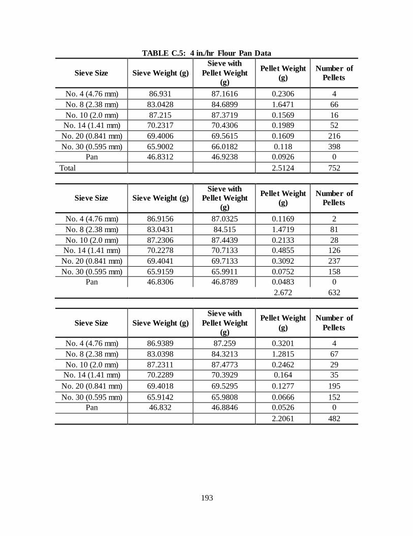
193
TABLE C.5: 4 in./hr Flour Pan Data
Sieve Size Sieve Weight (g)
Sieve with
Pellet Weight
(g)
Pellet Weight
(g)
Number of
Pellets
No. 4 (4.76 mm) 86.931 87.1616 0.2306 4
No. 8 (2.38 mm) 83.0428 84.6899 1.6471 66
No. 10 (2.0 mm) 87.215 87.3719 0.1569 16
No. 14 (1.41 mm) 70.2317 70.4306 0.1989 52
No. 20 (0.841 mm) 69.4006 69.5615 0.1609 216
No. 30 (0.595 mm) 65.9002 66.0182 0.118 398
Pan 46.8312 46.9238 0.0926 0
Total 2.5124 752
Sieve Size Sieve Weight (g)
Sieve with
Pellet Weight
(g)
Pellet Weight
(g)
Number of
Pellets
No. 4 (4.76 mm) 86.9156 87.0325 0.1169 2
No. 8 (2.38 mm) 83.0431 84.515 1.4719 81
No. 10 (2.0 mm) 87.2306 87.4439 0.2133 28
No. 14 (1.41 mm) 70.2278 70.7133 0.4855 126
No. 20 (0.841 mm) 69.4041 69.7133 0.3092 237
No. 30 (0.595 mm) 65.9159 65.9911 0.0752 158
Pan 46.8306 46.8789 0.0483 0
2.672 632
Sieve Size Sieve Weight (g)
Sieve with
Pellet Weight
(g)
Pellet Weight
(g)
Number of
Pellets
No. 4 (4.76 mm) 86.9389 87.259 0.3201 4
No. 8 (2.38 mm) 83.0398 84.3213 1.2815 67
No. 10 (2.0 mm) 87.2311 87.4773 0.2462 29
No. 14 (1.41 mm) 70.2289 70.3929 0.164 35
No. 20 (0.841 mm) 69.4018 69.5295 0.1277 195
No. 30 (0.595 mm) 65.9142 65.9808 0.0666 152
Pan 46.832 46.8846 0.0526 0 2.2061 482

194
TABLE C.6: 6 in./hr Flour Pan Method Data
Sieve Size Sieve Weight (g)
Sieve with
Pellet Weight
(g)
Pellet Weight
(g)
Number of
Pellets
No. 4 (4.76 mm) 86.9518 87.185 0.2332 3
No. 8 (2.38 mm) 83.0578 84.4492 1.3914 69
No. 10 (2.0 mm) 87.2372 87.5993 0.3621 65
No. 14 (1.41 mm) 70.2253 70.7432 0.5179 231
No. 20 (0.841 mm) 69.4028 69.7644 0.3616 377
No. 30 (0.595 mm) 65.8946 66.026 0.1314 283
Pan 46.8318 46.8934 0.0616 0
Total 2.9976 1028
Sieve Size Sieve Weight (g)
Sieve with
Pellet Weight
(g)
Pellet Weight
(g)
Number of
Pellets
No. 4 (4.76 mm) 86.9303 87.6492 0.7189 8
No. 8 (2.38 mm) 83.0389 85.444 2.4051 97
No. 10 (2.0 mm) 87.2422 87.8105 0.5683 99
No. 14 (1.41 mm) 70.2426 71.1175 0.8749 294
No. 20 (0.841 mm) 68.4026 69.8623 1.4597 342
No. 30 (0.595 mm) 65.8844 66.0875 0.2031 445
Pan 46.8305 46.9563 0.1258 0
6.23 1285
Sieve Size Sieve Weight (g)
Sieve with
Pellet Weight
(g)
Pellet Weight
(g)
Number of
Pellets
No. 4 (4.76 mm) 86.9353 87.1075 0.1722 2
No. 8 (2.38 mm) 83.05 85.0595 2.0095 90
No. 10 (2.0 mm) 87.2635 87.4822 0.2187 34
No. 14 (1.41 mm) 70.222 70.9371 0.7151 240
No. 20 (0.841 mm) 69.4265 69.9717 0.5452 515
No. 30 (0.595 mm) 65.8853 65.9968 0.1115 256
Pan 46.8238 46.9141 0.0903 0
3.7722 1137

195
TABLE C.7: Sandy Loam Soil Analysis
Sieve No. Sieve Size
(mm)
Mass of
Sieve (g)
Mass
Soil +
Sieve (g)
Mass of
Soil (g)
%
Retained
Cum.
Percent
Retained
4 4.750 0.0 0.0 0.00% 0.00% 100.00%
10 2.000 15.8 15.8 7.66% 7.66% 92.34%
20 0.841 30.9 15.1 7.32% 14.98% 85.02%
40 0.420 57.4 26.5 12.85% 27.82% 72.18%
80 0.177 102.5 45.1 21.86% 49.68% 50.32%
100 0.150 112.9 10.4 5.04% 54.73% 45.27%
200 0.075 142.5 29.6 14.35% 69.07% 30.93%
Pan 0.000 206.3 63.8 30.93% 100.00% 0.00%
Total: 206.3
Time,
min
Hydrometer
Reading, R Rcp % Finer Rcl L (cm) A D (mm)
% Finer
Total
0 0.075 30.93%
0.25 51 48.15 96.30 51 7.9 0.0133 0.075 29.78%
0.5 48 45.15 90.30 48 8.4 0.0133 0.055 27.93%
1 47 44.15 88.30 47 8.6 0.0133 0.039 27.31%
2 46 43.15 86.30 46 8.8 0.0133 0.028 26.69%
4 44 41.15 82.30 44 9.1 0.0133 0.020 25.45%
8 41 38.15 76.30 41 9.6 0.0133 0.015 23.60%
15 38 35.15 70.30 38 10.1 0.0133 0.011 21.74%
30 35 32.15 64.30 35 10.5 0.0133 0.008 19.89%
60 32 29.15 58.30 32 11.0 0.0133 0.006 18.03%
120 28 25.15 50.30 28 11.7 0.0133 0.004 15.56%
240 26 23.15 46.30 26 12.0 0.0133 0.003 14.32%
480 23 20.15 40.30 23 12.5 0.0133 0.002 12.46%
1440 21 18.15 36.30 21 12.8 0.0133 0.001 11.23%

196
Compacted Soil -Sample No. 1 2 3 4 5
Tin No. A-3 C-6 H-6 E-3 55
Tin Weight (g) 13.8 14.3 14.2 14.1 13.9
Moist Sample Weight + Tin (g) 87.3 86 97.5 96.6 96.5
Dry Sample Weight + Tin (g) 79.5 76.8 84.9 86.6 84.9
Moist Sample Weight (g) 73.5 71.7 83.3 82.5 82.6
Dry Sample Weight (g) 65.7 62.5 70.7 72.5 71
Mw = Mass of Pore Water (g) 7.8 9.2 12.6 10 11.6
W = Moisture Content 11.87% 14.72% 17.82% 13.79% 16.34%
Weight of Mold (g) 4279.4 4279.9 4281.4 4280.4 4281.4
Weight of Compacted Soil + Mold (g) 6160.9 6235 6183.7 6233.2 6207.4
Weight of Wet Soil in Mold (g) 1881.5 1955.1 1902.3 1952.8 1926
Wet Unit Weight (lb/ft3) 124.44 129.31 125.82 129.16 127.38
Dry Unit Weight of Compaction (lb/ft3) 111.23 112.72 106.78 113.50 109.49
Optimal Moisture Content 13.5% Optimal Compaction 113.6
Plastic Limit
Sample Number 1 2
Container No. F-9 BC
Mass Moist Soil + Container (g) 25.9 21.7
Mass Dry Soil + Container (g) 23.7 20.3
Mass Container (g) 14.1 14
Water Content (%) 22.92% 22.22%
Liquid Limit
Test Number 1 2 3
Container No. 56 F-A F-3
Mass Moist Soil + Container (g) 40.5 46.2 41.8
Mass Dry Soil + Container (g) 35 39.5 37
Mass Container (g) 14.2 14.1 14.1
Water Content (%) 32.83% 26.38% 20.96%
Number of Blows 18 26 34
Target Blows 15 - 25 20 - 30 25 - 35
Liquid Limit 31.55% 26.50% 21.76%

197
TABLE C.8: Loam Soil Analysis
Sieve No. Sieve Size
(mm)
Mass
of
Sieve
(g)
Mass
Soil +
Sieve (g)
Mass
of Soil
(g)
%
Retained
Cum.
Percent
Retained
% Finer
4 4.76 510.4 510.4 0 0.00% 0.00% 100.00%
10 2 488.7 489.4 0.7 0.77% 0.77% 99.23%
20 0.841 414 417.8 3.8 4.19% 4.96% 95.04%
40 0.42 466 474.2 8.2 9.04% 14.00% 86.00%
60 0.25 429.4 437.4 8 8.82% 22.82% 77.18%
100 0.149 334.7 342.8 8.1 8.93% 31.75% 68.25%
200 0.074 500.1 510.8 10.7 11.80% 43.55% 56.45%
Pan 0 362.4 362.8 51.2 56.45% 100.00% 0.00%
Total 90.7
Time
(min)
Hydrometer
Reading, R Rcp
%
Finer Rcl L (cm) A D (mm)
% Finer
Total
0 0.074 56.45%
0.25 51 49.9 98.23 51 7.9 0.0132 0.074 55.45%
0.5 49 47.9 94.29 49 8.3 0.0132 0.054 53.23%
1 46 44.9 88.39 46 8.8 0.0132 0.039 49.89%
2 43 41.9 82.48 43 9.2 0.0132 0.028 46.56%
4 40 38.9 76.57 40 9.7 0.0132 0.021 43.23%
8 35 33.9 66.73 35 10.6 0.0132 0.015 37.67%
15 31 29.9 58.86 31 11.2 0.0132 0.011 33.23%
30 26 24.9 49.02 26 12 0.0132 0.008 27.67%
60 23 21.9 43.11 23 12.5 0.0132 0.006 24.34%
120 19 17.9 35.24 19 13.2 0.0132 0.004 19.89%
240 16 14.9 29.33 16 13.7 0.0132 0.003 16.56%
360 13 11.9 23.43 13 14.2 0.0132 0.003 13.22%
480 12 10.9 21.46 12 14.3 0.0132 0.002 12.11%
1440 10 8.9 17.52 10 14.7 0.0132 0.0013 9.89%

198
Compacted Soil Sample Number 1 2 3 4 5
Tin Number 81 700 5 91 10
Tin Weight (g) 14.8 14.7 14.7 14.7 14.7
Moist Sample Weight + Tin (g) 53.7 52.4 61 56.9 58.6
Dry Sample Weight + Tin (g) 50.2 48.2 53.8 48.9 49.8
Moist Sample Weight (g) 38.9 37.7 46.3 42.2 43.9
Dry Sample Weight (g) 35.4 33.5 39.1 34.2 35.1
Mw = Mass of Pore Water (g) 3.5 4.2 7.2 8 8.8
W = Moisture Content 9.89% 12.54% 18.41% 23.39% 25.07%
Weight of Mold (g) 4283.8 4282.8 4280.1 4285 4291.4
Weight of Compacted Soil + Mold (g) 5737.5 5817.8 5987.5 6039.6 6014.9
Weight of Wet Soil in Mold (g) 1453.7 1535 1707.4 1754.6 1723.5
Wet Unit Weight (lb/ft3) 96.15 101.52 112.93 116.05 113.99
Dry Unit Weight of Compaction (lb/ft3) 87.50 90.21 95.36 94.05 91.14
Optimal Moisture Content 20.0% Maximum Compaction 96.0
Sample Number 1 2
Container No. 81 93
Mass Moist Soil + Container (g) 20.8 21
Mass Dry Soil + Container (g) 19.5 19.6
Mass Container (g) 14.7 14.9
Water Content (%) 27.08% 29.79%
Liquid Limit
Test Number 1 2 3
Container No. 5 42 12
Mass Moist Soil + Container (g) 26.6 29.3 53.1
Mass Dry Soil + Container (g) 24.0 24.9 47.3
Mass Container (g) 14.6 11.9 31.7
Water Content (%) 27.66% 33.85% 37.18%
Number of Blows 30 23 18
Target Blows 15 - 25 20 - 30 25 - 35
Liquid Limit 28.28% 33.51% 35.73%

199
TABLE C.9: Sandy Loam Bare Soil Test
Date: 9/12/18 Weather During Calibration
Operator: BF Temperature: 75 F
Operating Pressure: 31 psi Average wind speed: 0.20 mph
Test Intensity: 4.08 in/hr Max wind speed: 0.40 mph
Test Start Time: 9:35 Wind Direction: W Test Finish Time: 10:35 Humidity 81 %
Drive Cylinder Compaction Data
Cylinder Number 1 2 3
Test Location Number 26 16 43
Thickness of Soil Sample (in) 1.05 0.90 0.95
Volume of Drive Cylinder (in3) 216.11 185.24 195.53
Wet Weight of Pan and Soil (g) 435 410 435
Dry Weight of Pan and Soil (g) 390 360 385
Weight of Pan (g) 55 60 55
Moisture Lost (g) 45 50 50
Dry Weight of Soil (g) 335 300 330
Water Content (%) 13.43 16.67 15.15
Wet Density (g/cm3) 1.7583 1.8894 1.9434
Dry Density (g/ cm33) 1.5501 1.6195 1.6877
Maximum Dry Density (g/ cm3) 113.6 113.6 113.6
Optimum Water Content (%) 13.30 13.30 13.03
Percent Compacted (%) 85.1 89.0 82.7
Collected Sediment Loss
Sample Number 1 2 3 4
Settling Time (min) 60 60 60 60
Total Wet Weight of Sediment, lb 711.6 114.8 346.4 110.9
Container Weight, lb 46 4.6 16.1 6.9
Wet Weight + Container , lb 757.6 119.4 362.5 117.8
Dry Weight, lb 287.6681 92.78356 269.6805 75.54058
Moisture Content, % 59.57% 19.18% 22.15% 31.88%
Average Moisture Content, % 33.20%
Total Dry Weight of Sediment, lb 725.67

200
TSS and Turbidity Data
Sample
ID
Time
(min)
Dilution
Factor
Turbidity
Reading
(NTU)
Filter +
Crinkle
Dish (g)
Dry Filter
+ Soil +
Crinkle
Dish (g)
Original Sample
Turbidity
(NTU)
TSS
(mg/L)
2801 3 128 816 1.3971 1.413 104448 81408
2802 6 128 491 1.365 1.3763 62848 57856
2803 9 128 343 1.3904 1.3976 43904 36864
2804 12 128 326 1.3739 1.3794 41728 28160
2805 15 64 596 1.3703 1.3825 38144 31232
2806 18 64 626 1.385 1.3986 40064 34816
2807 21 64 528 1.3882 1.3976 33792 24064
2808 24 64 903 1.3901 1.4088 57792 47872
2809 27 64 956 1.3677 1.3891 61184 54784
2810 30 128 503 1.3746 1.3846 64384 51200
2811 33 128 538 1.3888 1.4004 68864 59392
2812 36 128 624 1.3825 1.3943 79872 60416
2901 39 128 690 1.3704 1.3834 88320 66560
2902 42 128 789 1.3797 1.3965 100992 86016
2903 45 128 735 1.3668 1.381 94080 72704
2904 48 128 423 1.371 1.3862 54144 77824
2905 51 128 589 1.385 1.3967 75392 59904
2906 54 128 591 1.3775 1.3926 75648 77312
2907 57 128 623 1.3791 1.3912 79744 61952
2908 60 128 504 1.3743 1.3835 64512 47104
(a) Test 1 Turbidity Results (b) Test 1 TSS Results
Water Quality Results.
0
20,000
40,000
60,000
80,000
100,000
120,000
0 20 40 60
Turb
idit
y
(NT
U)
Time (min)
0
20,000
40,000
60,000
80,000
100,000
0 20 40 60
TS
S (
mg/L
)
Time (min)

201
TABLE C.10: Loose Straw Test Data
Date: 11/30/18 Weather During Calibration
Operator: BF Temperature: 60 F
Operating Pressure: 32 psi Average wind speed: 0.2 mph
Test Intensity: 4.07 in/hr Max wind speed: 0.1 mph
Test Start Time: 8:46 Wind Direction: SSE Test Finish Time: 9:50 Humidity 60 %
Drive Cylinder Compaction Data
Cylinder Number 1 2 3
Test Location Number 5 26 52
Thickness of Soil Sample (in) 1.0 0.70 0.55
Volume of Drive Cylinder (in3) 205.82 144.08 113.20
Wet Weight of Pan and Soil (g) 515 410 355
Dry Weight of Pan and Soil (g) 467.4 371.4 328.2
Weight of Pan (g) 150 150 145
Moisture Lost (g) 47.6 38.6 26.8
Dry Weight of Soil (g) 317.4 221.4 183.2
Water Content (%) 15.0 17.43 14.63
Wet Density (g/cm3) 1.7734 1.8046 1.8551
Dry Density (g/ cm33) 1.5421 1.5367 1.6183
Maximum Dry Density (g/ cm3) 113.6 113.6 113.6
Optimum Water Content (%) 13.30 13.30 13.30
Percent Compacted (%) 84.7 84.4 88.9
Collected Sediment Loss
Sample Number 1 2
Settling Time (hr) 24 24
Total Wet Weight of Sediment, lb 55.2 231.3
Container Weight, lb 2 16.1
Wet Weight + Container , lb 57.2 247.4
Dry Weight, lb 40.35 72.71
Moisture Content, % 26.91% 68.56%
Average Moisture Content, % 47.74%
Total Dry Weight of Sediment, lb 113.06

202
TSS and Turbidity Data
Sample
ID
Time
(min)
Dilution
Factor
Turbidity
Reading
(NTU)
Filter +
Crinkle
Dish (g)
Dry Filter
+ Soil +
Crinkle
Dish (g)
Original Sample
Turbidity
(NTU)
TSS
(mg/L)
101 3 4 748 1.4014 1.4274 2992 4160
102 6 32 620 1.3682 1.3756 19840 9472
103 9 64 543 1.3953 1.401 34752 14592
104 12 32 349 1.3808 1.3847 11168 4992
105 15 32 310 1.3747 1.3797 9920 6400
106 18 32 356 1.3908 1.3979 11392 9088
107 21 32 515 1.3929 1.4024 16480 12160
108 24 32 752 1.3962 1.4071 24064 13952
109 27 32 539 1.3733 1.3823 17248 11520
110 30 32 546 1.3798 1.3886 17472 11264
111 33 32 714 1.3944 1.405 22848 13568
112 36 32 579 1.3891 1.3988 18528 12416
113 39 32 761 1.3765 1.3884 24352 15232
114 42 32 682 1.3766 1.3868 21824 13056
115 45 32 405 1.3683 1.374 12960 7296
116 48 32 403 1.3949 1.4024 12896 9600
117 51 32 577 1.3692 1.3777 18464 10880
118 54 32 633 1.3938 1.4028 20256 11520
119 57 32 512 1.3908 1.3984 16384 9728
120 60 32 413 1.3834 1.3901 13216 8576
(a) Test 1 Turbidity Results (b) Test 1 TSS Results
0
5,000
10,000
15,000
20,000
25,000
30,000
35,000
40,000
0 20 40 60
Turb
idit
y
(NT
U)
Time (min)
0
2,000
4,000
6,000
8,000
10,000
12,000
14,000
16,000
0 20 40 60
TS
S (
mg/L
)
Time (min)

203
TABLE C.11: Loam Bare Soil Raw Data
Date: 3/9/20 Weather During Calibration Operator: BF Temperature: 52 F
Operating Pressure: 26 psi Average wind speed: 0.43 mph Test Intensity: 4.08 in/hr Max wind speed: 0.75 mph
Test Start Time: 9:21 Wind Direction: ESE Test Finish Time: 10:37 Humidity 78 %
Drive Cylinder Compaction Data
Cylinder Number 1 2 3
Test Location Number 13 27 41
Thickness of Soil Sample (in) 1.05 1.35 1.55
Volume of Drive Cylinder (in3) 216.11 277.86 319.02
Wet Weight of Pan and Soil (g) 900 990 1055
Dry Weight of Pan and Soil (g) 830 905 975
Weight of Pan (g) 530 530 530
Moisture Lost (g) 70 85 80
Dry Weight of Soil (g) 300 375 445
Water Content (%) 23.33 22.67 17.98
Wet Density (g/cm3) 1.7121 1.6555 1.6456
Dry Density (g/cm3) 1.3882 1.3496 1.3949
Maximum Dry Density (g/cm3) 96.0 96.0 96.0
Optimum Water Content (%) 20.0 20.0 20.0
Percent Compacted (%) 90.2 87.7 90.7
Collected Sediment Loss
Sample Number 2 in/hr 4 in/hr 6 in/hr
Settling Time (hr) 24 24 24 24 24 24 24
Total Wet Weight of Sediment (lb) 66 212.6 518.6 213.6 674.9 467.1 771
Container Weight (lb) 6.6 13.2 37.4 12 41.8 28.6 44
Dry Weight (lb) 28.65 106.30 330.74 213.60 359.28 333.32 500.87
Moisture Content (% ) 56.59 50.00 36.22 34.39 46.77 28.64 35.04
Average Moisture Content (% ) 56.59 40.20 36.81
Total Dry Weight of Sediment (lb) 28.65 650.64 1193.46

204
TSS and Turbidity Data
Sample
ID
Time
(min)
Dilution
Factor
Turbidity
Reading
(NTU)
Filter +
Crinkle
Dish
(g)
Dry Filter
+ Soil +
Crinkle
Dish (g)
Original Sample
Turbidity
(NTU)
TSS
(mg/L)
1 3 64 950 1.3763 1.3959 60800 50176
2 6 128 586 1.3849 1.3984 75008 69120
3 9 128 404 1.3797 1.3897 51712 51200
4 12 128 365 1.3786 1.3880 46720 48128
5 15 128 299 1.3856 1.3956 38272 51200
6 18 128 286 1.3774 1.3859 36608 43520
7 21 128 325 1.3776 1.3854 41600 39936
8 24 128 361 1.3807 1.3896 46208 45568
9 27 128 302 1.3825 1.3906 38656 41472
10 30 128 324 1.3962 1.4038 41472 38912
11 33 128 298 1.4004 1.4073 38144 35328
12 36 128 280 1.3897 1.3964 35840 34304
13 39 128 323 1.3760 1.3851 41344 46592
14 42 128 282 1.3907 1.3987 36096 40960
15 45 128 425 1.3733 1.3836 54400 52736
16 48 128 478 1.3769 1.3921 61184 77824
17 51 128 588 1.3651 1.3823 75264 88064
18 54 256 305 1.3857 1.3913 78080 57344
19 57 128 504 1.3917 1.4049 64512 67584
20 60 128 736 1.3817 1.3962 94208 74240
(a)bare soil turbidity results (b) bare soil TSS results
0
10,000
20,000
30,000
40,000
50,000
60,000
70,000
80,000
90,000
100,000
0 20 40 60
Turb
idit
y
(NT
U)
Time (min)
0
20,000
40,000
60,000
80,000
100,000
0 20 40 60
TS
S (
mg/L
)
Time (min)

205
Discharge over Time
0
5
10
15
20
0 20 40 60
Dis
charg
e (
gal/
min
)
Time (min)

206
TABLE C.12: Curlex I Test Results
Date: 1/31/20 Weather During Calibration
Operator: BF Temperature: 58 F
Operating Pressure: 28 psi Average wind speed: 0.48 mph
Test Intensity: 4.05 in/hr Max wind speed: 0.8 mph
Test Start Time: 1:26 Wind Direction: NE Test Finish Time: 2:38 Humidity 31 %
Drive Cylinder Compaction Data
Cylinder Number 1 2 3
Test Location Number 29 4 54
Thickness of Soil Sample (in) 0.95 1.25 1.45
Volume of Drive Cylinder (in3) 195.53 257.28 298.44
Wet Weight of Pan and Soil (g) 475 565 645
Dry Weight of Pan and Soil (g) 425 505 565
Weight of Pan (g) 155 150 160
Moisture Lost (g) 50 60 80
Dry Weight of Soil (g) 270 355 405
Water Content (%) 18.52 16.90 19.75
Wet Density (g/cm3) 1.6366 1.6130 1.6251
Dry Density (g/ cm33) 1.3809 1.3798 1.3571
Maximum Dry Density (g/ cm3) 96.0 96.0 96.0
Optimum Water Content (%) 20.0 20.0 20.0
Percent Compacted (%) 89.8 89.7 88.2
Collected Sediment Loss
Sample Number 2 in/hr 4 in/hr 6 in/hr
Settling Time (hr) 24 24 24 24
Total Wet Weight of Sediment (lb) 19.6 67.8 189.6 124
Container Weight (lb) 2.2 4.6 13.2 6.6
Dry Weight (lb) 1.70 15.84 7.39 61.23
Moisture Content (%) 91.30 76.64 96.10 50.62
Average Moisture Content (%) 91.30 76.64 73.36
Total Dry Weight of Sediment (lb) 1.70 15.84 68.62

207
TSS and Turbidity Data
Sample
ID
Time
(min)
Dilution
Factor
Turbidity
Reading
(NTU)
Filter +
Crinkle
Dish (g)
Dry Filter
+ Soil +
Crinkle
Dish (g)
Original Sample
Turbidity
(NTU)
TSS
(mg/L)
3 0 0 0.0000 0.0000 0 0
1 6 16 471 1.3791 1.3890 7536 6336
2 9 32 467 1.3900 1.4020 14944 15360
3 12 32 347 1.3825 1.3914 11104 11392
4 15 32 251 1.3822 1.3889 8032 8576
5 18 16 602 1.3897 1.4060 9632 10432
6 21 16 706 1.3811 1.3991 11296 11520
7 24 16 665 1.3815 1.4022 10640 13248
8 27 16 580 1.3857 1.4042 9280 11840
9 30 16 612 1.3867 1.4065 9792 12672
10 33 16 496 1.4001 1.4166 7936 10560
11 36 16 549 1.4048 1.4228 8784 11520
12 39 16 565 1.3955 1.4126 9040 10944
13 42 16 837 1.3797 1.4042 13392 15680
14 45 16 669 1.3942 1.4154 10704 13568
15 48 16 749 1.3791 1.4009 11984 13952
16 51 16 773 1.3818 1.4045 12368 14528
17 54 16 675 1.3722 1.3936 10800 13696
18 57 16 687 1.3921 1.4121 10992 12800
19 60 16 805 1.3972 1.4203 12880 14784
(a) Test 1 Turbidity Results (b) Test 1 TSS Results
0
2,000
4,000
6,000
8,000
10,000
12,000
14,000
16,000
0 20 40 60
Turb
idit
y
(NT
U)
Time (min)
0
5,000
10,000
15,000
20,000
0 20 40 60
TS
S (
mg/L
)
Time (min)

208
Discharge over Time
0
2
4
6
8
10
12
14
16
18
0 20 40 60
Dis
charg
e (
gal/m
in)
Time (min)

209
TABLE C.13: R-factor and K-factor Calculations
Target
Storm
Event
Gauge
Reading
(in.)
Rainfall
(in.)
Test
Intensity
(in./hr)
Particle
Diameter
Range (mm)
Average
raindrop
size (mm)
% of
rainfall
Fall
Vel
(m/s)
Fall Vel
(ft/s)
2 in/hr
0.7
0.77 2.30
4.76+ 6.03 3.95% 7.79 25.57
0.8 4.76-2.38 3.79 55.36% 7.38 24.21
0.9 2.38-2.0 2.50 10.10% 6.38 20.92
0.8 2.0-1.41 1.81 19.39% 5.61 18.42
0.7 1.41-0.841 1.21 8.93% 4.83 15.85
0.7 0.841-0.59 0.91 2.27% 4.39 14.39
Average 0.77 100.00%
4 in/hr
2
1.32 3.95
4.76+ 5.29 9.56% 7.84 25.73
2.2 4.76-2.38 3.52 60.59% 7.22 23.68
2.3 2.38-2.0 2.59 8.23% 6.47 21.22
2.1 2.0-1.41 2.00 11.03% 5.84 19.16
2 1.41-0.841 1.21 7.38% 4.82 15.81
1.9 0.841-0.59 0.89 3.21% 4.35 14.27
Average 2.08 100.00%
6 in/hr
4
2.10 6.30
4.76+ 5.78 9.33% 7.83 25.69
4.1 4.76-2.38 3.65 46.08% 7.29 23.93
4.3 2.38-2.0 2.28 8.70% 6.15 20.17
4.4 2.0-1.41 1.76 15.53% 5.55 18.22
4.4 1.41-0.841 1.55 17.20% 5.29 17.36
3.9 0.841-0.59 0.95 3.16% 4.45 14.59
Average 4.18 100.00%

210
Target
Storm Event
Rainfall
Vol (ft3)
Rainfall
Weight (lbf)
Rainfall
Mass (slugs)
Incr.
Rainfall
Mass
(slugs)
KErainfall
(ft-lbf)
KEtotalrainfall
(ft-tonf)
Incremental
E (ft-tonf/acre)
E
(hundred ft-tons/ac)
2 in/hr 20.44 1275.73 39.62
1.56 511.28 0.26 34.80 0.35
21.93 6426.04 3.21 437.37 4.37
4.00 875.27 0.44 59.57 0.60
7.68 1303.61 0.65 88.73 0.89
3.54 443.98 0.22 30.22 0.30
0.90 93.19 0.05 6.34 0.06
Average 39.619 9653.38 4.83 657.03 6.57
4 in/hr 35.11 2190.93 68.04
6.51 2152.83 1.08 146.53 1.47
41.23 11554.66 5.78 786.44 7.86
5.60 1260.64 0.63 85.80 0.86
7.50 1377.81 0.69 93.78 0.94
5.02 627.95 0.31 42.74 0.43
2.18 222.17 0.11 15.12 0.15
Average 68.041 17196.07 8.60 1170.41 11.70
6 in/hr 56.00 3494.40 108.52
10.12 3340.87 1.67 227.39 2.27
50.00 14311.37 7.16 974.07 9.74
9.44 1920.78 0.96 130.73 1.31
16.85 2798.99 1.40 190.51 1.91
18.67 2813.48 1.41 191.49 1.91
3.43 365.41 0.18 24.87 0.25
Average 108.522 25550.89 12.78 1739.06 17.39

211
Target
Storm Event
Incremental
E (hundred
ft-tons/ac)
I30
(in./hr)
Incremental
EI30
Soil Loss
per
Intensity (lb)
Soil Loss
per
Intentisty (ton)
A
(ton/ac)
2 in/hr 6.57 2.30 15.11 28.65 0.01 1.95
Average
4 in/hr 18.27 3.40 62.13 650.64 0.33 46.23
Average
6 in/hr 35.66 5.52 196.75 1193.46 0.60 127.46
Average
Slope Intercept
y = 0.6716 -2.7923
x = 182.02
y = 119.46
K = A/RLSCP K-factor uses slope of
regression line and
theoretical R to normalize it for normalized
C-factor calculations
A = 119.46
Theoretical R = 182.02
LS Factor = 2.86
C = 1
P = 1
A/R = 0.672
K = 0.23
y = 0.6716x - 2.7923R² = 0.9894
0
20
40
60
80
100
120
140
0 20 40 60 80 100 120 140 160 180 200 220
A (
ton/a
c)
R-Factor

212
TABLE C.14: C-factor Calculations
Target
Storm
Event
Gauge
Reading
(in.)
Incremental
E (hundred
ft-tons/ac)
I30
(in./hr)
Incremental
EI30
Soil
Loss (lb)
per
Intensity
Soil
Loss
(ton) per
Intensity
A
(ton/ac)
Control
Soil Loss
for
Test's
Cum. R-Factor
C
Factor
(using
control)
C
Factor
(using
RUSLE
Equ.)
2 in/hr
0.7
6.14 2.15 13.20 1.70 0.00 0.12 8.87 0.01 0.0130
0.7
0.8
0.8
0.6
0.7
Average 0.72
4 in/hr
1.9
18.14 3.42 61.99 15.84 0.01 1.19 41.63 0.03 0.0287
2.2
2.2
2.2
1.9
2
Average 2.07
6 in/hr
3.8
34.57 5.32 183.78 68.62 0.03 5.86 123.43 0.05 0.0475
4.1
4.3
4.2
3.9
4
Average 4.05
y = 0.0346x - 0.595R² = 0.9892
0
1
2
3
4
5
6
7
0 50 100 150 200
A (
ton
/ac)
R-Factor

213
Test
Rainfall Data Soil Loss Data RUSLE Calculations
Target
Intensity
(in./hr)
Depth
(in.)
Actual
Intensity
(in./hr)
Soil
Loss
(lbs)
Soil Loss
(ton)
Soil Loss
(ton/acre)
Cumm.
Soil
Loss
Ratio
Cumm.
A
(ton/ac)
Incremental
R - Factor
Control Soil
Loss for
Test's Cum.
R-Factor
(ton/acre)
K-
Factor
LS-
Factor
C -
Factor
per
Intensity
from
actual
soil loss
A
Control
2 0.77 2.30 28.65 0.01 1.95 N/A 1.95 15.11 N/A
0.23 2.86
N/A 4 1.32 3.95 650.64 0.33 46.23 N/A 48.18 62.13 N/A
6 2.10 6.30 1193.46 0.60 127.46 N/A 175.65 196.75 N/A
Test 1
2 0.72 2.15 1.70 0.00 0.12 0.01 0.12 13.20 8.87 0.0130
4 1.35 4.05 15.84 0.01 1.19 0.03 1.19 61.99 41.63 0.0287
6 1.98 5.95 68.62 0.03 5.86 0.05 5.86 183.78 123.43 0.0475
Test 2
2 0.70 2.10 4.49 0.00 0.31 0.04 0.31 12.60 8.46 0.0361
4 1.37 4.10 25.16 0.01 2.02 0.05 2.02 62.31 41.85 0.0482
6 2.00 6.00 67.25 0.03 6.60 0.05 6.60 186.28 125.11 0.0527
Test 3
2 0.72 2.15 3.21 0.00 0.22 0.02 0.22 13.20 8.87 0.0246
4 1.37 4.10 18.25 0.01 1.46 0.03 1.46 63.10 42.38 0.0345
6 2.03 6.10 65.53 0.03 5.92 0.05 5.92 190.87 128.19 0.0462
Average C-Factor = 0.0488

214
CONTROL
Slope Intercept
y = 0.6716 -2.7923
x = 182.02
K = A/RLSCP
A = 119.46
Theoretical R = 182.02
LS Factor = 2.86
C = 1
P = 1
A/R = 0.671
K = 0.23
TEST 1
Test 1 Slope Intercept
y = 0.0346 -0.5950
x = 182.02
C = A/RKLSP
A = 5.70
Theoretical R = 182.02
LS Factor = 2.86
K = 0.23
P = 1.00
A/R = 0.0345
C = 0.05
TEST 2
Test 2 Slope Intercept
y = 0.0363 -0.1917
x = 182.02
C = A/RKLSP
A = 6.42
Theoretical R = 182.02
LS Factor = 2.86
K = 0.23
P = 1.00
A/R = 0.0363
C = 0.05
TEST 3
Test 3 Slope Intercept
y = 0.0327 -0.3746
x = 182.02
C = A/RKLSP
A = 5.57
Theoretical R = 182.02
LS Factor = 2.86
K = 0.23
P = 1.00
A/R = 0.032652
C = 0.05

215
(a) Bare Soil (b) Curlex I Test 1
(c) Curlex I Test 2 (d) Curlex I Test 3
y = 0.6716x - 2.7923
R² = 0.9894
0
20
40
60
80
100
120
140
0 25 50 75 100 125 150 175 200 225
A (
ton
/ac)
R - Factor
y = 0.0346x - 0.595
R² = 0.9892
0
10
20
30
40
50
60
70
80
90
100
0 25 50 75 100 125 150 175 200
A (
ton
/ac)
R - Factor
y = 0.0363x - 0.1917
R² = 0.9998
0
10
20
30
40
50
60
70
80
90
100
0 25 50 75 100 125 150 175 200
A (
ton
/ac)
R - Factor
y = 0.0327x - 0.3746
R² = 0.9955
0
10
20
30
40
50
60
70
80
90
100
0 25 50 75 100 125 150 175 200 225
A (
ton
/ac)
R - Factor