evaluation of a cfd method for estimating aerodynamic loads
DESCRIPTION
determination of cfd loads using cfdTRANSCRIPT
Evaluation of a CFD method for
estimating aerodynamic loads on
external stores on JAS 39 Gripen
Jakob Ohrman
A thesis submitted in partial fulfilment
of the requirements for the degree of
Master of Science in Engineering Physics
Supervisor: Elisabeth Loven
Examiner: Mats G. Larson
May 22, 2011
Umea UniversityDepartment of Physics
SE-901 87 UMEASWEDEN

Abstract
Loads determination for external stores on fighter aircraft is an important task for manufac-turers in ensuring the safe operation of their aircraft. Due to the large number of possiblestore combinations, wind tunnel tests – the primary approach to obtaining loads data – can-not be performed for all configurations. Instead, supplementary techniques to estimatingloads are necessary. One approach is to use information from another store and adapt it,using so-called scaling methods, to the non-tested store.
In this thesis, a scaling method combining the results of computational fluid dynamics(CFD) simulations, for both a non-tested and a reference store, with existing wind tunneldata for the reference store, is thoroughly examined for a number of different stores, anglesof attack, sideslip angles and Mach numbers. The performance of the proposed scalingmethod is assessed in relation to currently used scaling methods, using non-parametric andmultivariate statistics.
The results show no definitive improvement in performance for the proposed scaling methodover the current methods. Although the proposed method is slightly more conservative,considerable variability in the estimates and an increased time consumption for scalingleads the author to advise against using the proposed method for scaling aerodynamic loadson external stores.
Keywords: aerodynamic loads, CFD, computational fluid dynamics, simulation, aircraft,external stores, scaling, Saab Aerosystems, JAS 39 Gripen

Sammanfattning
Lastbestamning for yttre utrustning pa stridsflygplan ar en viktig uppgift for att tillverkarnaska kunna garantera sakerheten for sina flygplan. Da antalet mojliga utrustningskombina-tioner ar mycket stort, kan inte vindtunneltester – normalt den framsta metoden for atterhalla lastdata – utforas for alla konfigurationer. Saledes behovs kompletterande metoderfor att skatta laster. Ett alternativ ar att anvanda data fran en annan utrustning ochanpassa den, med hjalp av sa kallade skalningsmetoder, till den icke-testade utrustningen.
I detta examensarbete behandlas en skalningsmetod som kombinerar resultaten fran nu-meriska stromningsberakningar – sa kallade CFD-simuleringar – for bade en testad och enicke-testad utrustning med befintliga vindtunneldata for den testade utrustningen. Metodenundersoks grundligt for ett antal olika utrustningar, anfallsvinklar, sidanblasningsvinklaroch Machtal. Prestandan hos den foreslagna skalningsmetoden utvarderas i relation till nuanvanda skalningsmetoder, baserat pa icke-parametrisk och multivariat statistik.
Resultaten visar inga definitiva forbattringar av prestanda for den foreslagna skalningsme-toden jamfort med de nuvarande metoderna. Aven om den foreslagna metoden ar nagotmer konservativ, sa foranleder betydande variationer i skattningar och en okad tidsatgangfor skalning forfattaren att avrada fran att anvanda den foreslagna metoden for skalning avluftlaster pa yttre utrustning.
Nyckelord: aerodynamik, luftlaster, CFD, numerisk stromningsmekanik, simulering, flyg-plan, yttre utrustning, skalning, Saab Aerosystems, JAS 39 Gripen

iv
v
Acknowledgments
First and foremost, I would like to express my deep gratitude to my supervisor, ElisabethLoven, for assisting and supporting me throughout the project. Together with her lovelycolleague Jenny Poovi, Elisabeth also provided me both with an insight into the subtle art ofloads determination for external stores and with a great and friendly workplace atmospherewith lots of laughter. It has truly been a pleasure being part of the Norrlandic corner of theoffice and I wish to thank both Elisabeth and Jenny for this.
I am very grateful to Adel Chebat and Bengt Mexnell for letting me share their deep knowl-edge of loads and loads determination and for having so many of my questions answered. Iwould also like to thank Jeremy Vandermeeren, from the Delft University of Technology, forhis many suggestions and all the interesting conversations on the afternoon bus home fromwork. Furthermore, I would like to acknowledge Gustav Johansson for his excellent work inpreparing the models used in the study. His store models served as a great foundation forthe modeling work done in this thesis and his contribution truly deserves a mention.
My most profound gratitude goes to Erica Amundsson at STARCS (formerly at Lutab),whose support and advice in the field of CFD simulations proved invaluable in managing toget the simulations done. Without her assistance in solving many of the problems that wereencountered, this thesis would not have been finished yet in many weeks. I am sincerelythankful that she put up with my continual visits and guided me through the CFD jungle.
I would also like to send my regards to Sofia, Emma, Mickael, Lena and all the otheremployees at the Loads Department and the Structural Dynamics, Flutter & SeparationDepartment at Saab Aerosystems. Many of you have assisted me with minor, but important,tasks and I would like to thank you for your help, but most of all you have made me enjoy thetime I have spent at Saab Aerosystems. Thank you, everyone, for your warm friendliness!
Dearest Caroline, You make me feel proud of my achievements and you stand by my sidewhen things fall apart. Your patience, your strength and your loving support have meanteverything to me during my time here at Saab. I could not have done this without you.
Linkoping, February 2011Jakob Ohrman

vi
vii
Contents
1 Introduction 1
2 Problem Description 3
2.1 Objectives . . . . . . . . . . . . . . . . . . . . . . . . . . . . . . . . . . . . . . 3
2.2 Purposes . . . . . . . . . . . . . . . . . . . . . . . . . . . . . . . . . . . . . . . 4
2.3 Related Work . . . . . . . . . . . . . . . . . . . . . . . . . . . . . . . . . . . . 4
2.3.1 Current Scaling Methods . . . . . . . . . . . . . . . . . . . . . . . . . 4
2.3.2 Proposed Scaling Method . . . . . . . . . . . . . . . . . . . . . . . . . 5
3 Theory and Methods 7
3.1 Definitions . . . . . . . . . . . . . . . . . . . . . . . . . . . . . . . . . . . . . . 7
3.2 Principles and Theory of the Scaling Methodology . . . . . . . . . . . . . . . 10
3.2.1 Modeling . . . . . . . . . . . . . . . . . . . . . . . . . . . . . . . . . . 10
3.2.2 Preprocessing . . . . . . . . . . . . . . . . . . . . . . . . . . . . . . . . 11
3.2.3 Simulation . . . . . . . . . . . . . . . . . . . . . . . . . . . . . . . . . 15
3.2.4 Post-Processing . . . . . . . . . . . . . . . . . . . . . . . . . . . . . . . 17
3.3 Procedures and Tools of the Study . . . . . . . . . . . . . . . . . . . . . . . . 20
3.3.1 Experimental Design and Data Acquisition . . . . . . . . . . . . . . . 20
3.3.2 Geometric Modeling and Mesh Generation . . . . . . . . . . . . . . . . 22
3.3.3 Preprocessing, Simulation and Post-Processing . . . . . . . . . . . . . 24
3.3.4 Scaling with Current Methods . . . . . . . . . . . . . . . . . . . . . . 25
3.3.5 Data Analysis and Assessment of Method Performance . . . . . . . . . 26
viii CONTENTS
4 Results 31
4.1 Preprocessing, Simulation and Post-processing . . . . . . . . . . . . . . . . . 31
4.2 Scaling . . . . . . . . . . . . . . . . . . . . . . . . . . . . . . . . . . . . . . . . 35
4.3 Data Analysis . . . . . . . . . . . . . . . . . . . . . . . . . . . . . . . . . . . . 35
5 Conclusions 43
5.1 Scaling Method Performance and Limitations . . . . . . . . . . . . . . . . . . 43
5.2 Recommendations . . . . . . . . . . . . . . . . . . . . . . . . . . . . . . . . . 45
5.3 Further Work . . . . . . . . . . . . . . . . . . . . . . . . . . . . . . . . . . . . 46
References 49
A Supplementary Data 51
A.1 ANOVA Results . . . . . . . . . . . . . . . . . . . . . . . . . . . . . . . . . . 51
ix
List of Figures
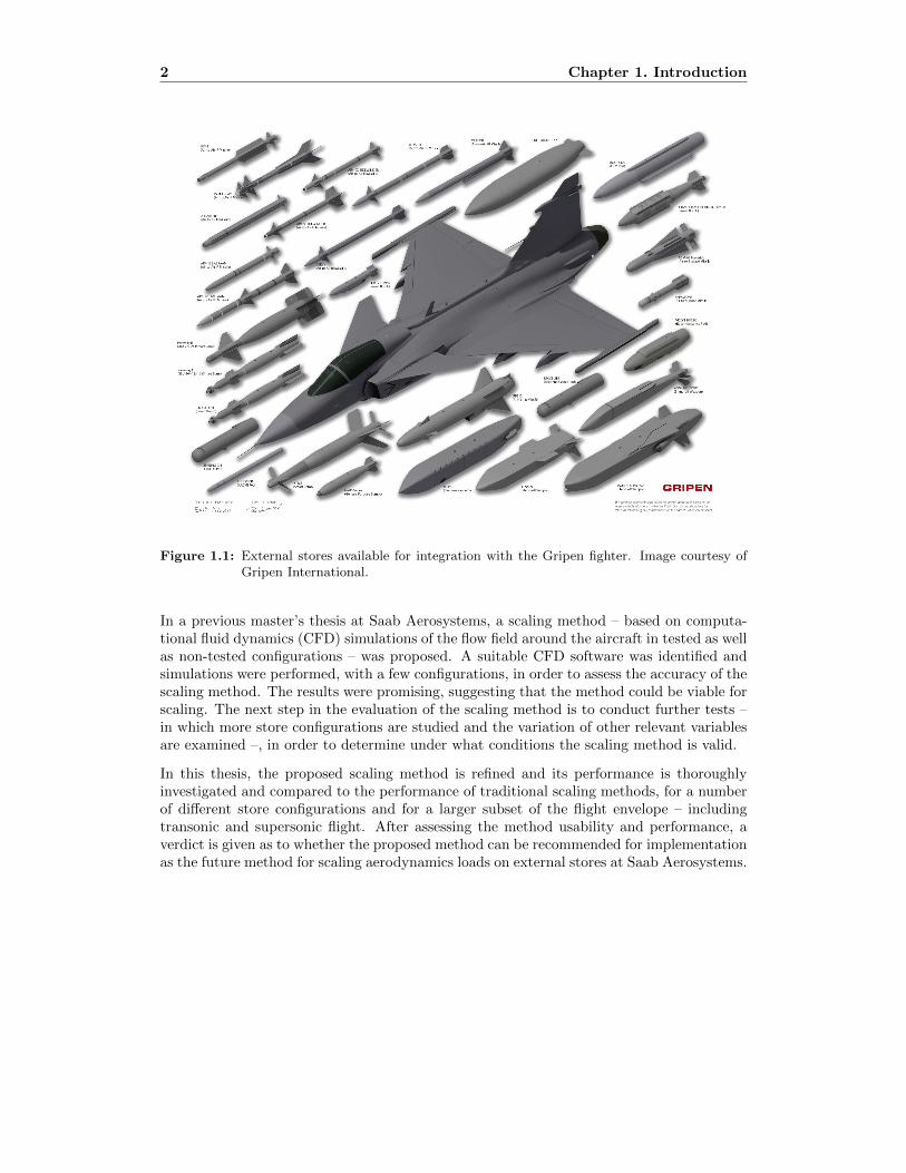
1.1 External stores available for integration with the Gripen fighter. . . . . . . . 2
3.1 Coordinate system and definitions of positive directions of forces, moments
and angles. . . . . . . . . . . . . . . . . . . . . . . . . . . . . . . . . . . . . . 8
3.2 The main steps in the work process of the investigated scaling methodology. . 10
3.3 Modeling in sumo: the positioning of a store in an integrated model consisting
of aircraft, pylons and stores. . . . . . . . . . . . . . . . . . . . . . . . . . . . 11
3.4 Mesh generation in sumo: surface mesh of a store and a pylon, with a dialog
for adjusting mesh parameters. . . . . . . . . . . . . . . . . . . . . . . . . . . 12
3.5 A Delaunay triangulation in the plane. . . . . . . . . . . . . . . . . . . . . . . 13
3.6 Mesh generation in sumo: cut plane of a TetGen volume mesh for an inte-
grated model consisting of aircraft, pylons and stores. . . . . . . . . . . . . . 14
3.7 Simulation in Edge: convergence plots of residuals and integrated loads as
functions of iteration number. . . . . . . . . . . . . . . . . . . . . . . . . . . . 19
3.8 Visualization in EnSight : streamlines for flow passing store and pressure on
surface of aircraft, pylons and store. . . . . . . . . . . . . . . . . . . . . . . . 20
3.9 Modeling in sumo: all modeled pylons. . . . . . . . . . . . . . . . . . . . . . . 23
3.10 Modeling in sumo: integrated model of the aircraft and all modeled pylons. . 23
3.11 Properties by which scaling method performance was measured. . . . . . . . . 27
4.1 Raw CFD force coefficient data (CC,CFD, CN,CFD) for two α sweeps, obtained
from Edge simulation runs. . . . . . . . . . . . . . . . . . . . . . . . . . . . . 33
4.2 Raw CFD moment coefficient data (CMX,CFD, CMY,CFD, CMZ,CFD) for two
α sweeps, obtained from Edge simulation runs. . . . . . . . . . . . . . . . . . 34

x LIST OF FIGURES
4.3 Estimates of force coefficient data (CC , CN ) for two α sweeps, obtained by
scaling. . . . . . . . . . . . . . . . . . . . . . . . . . . . . . . . . . . . . . . . 36
4.4 Estimates of moment coefficient data (CMX , CMY , CMZ) for two α sweeps,
obtained by scaling. . . . . . . . . . . . . . . . . . . . . . . . . . . . . . . . . 37
4.5 Histograms showing distribution of deviations (Di), for CC and CMY , in all
scalings performed. . . . . . . . . . . . . . . . . . . . . . . . . . . . . . . . . . 38
4.6 95% bootstrap confidence intervals for the properties by which scaling method
performance was measured. . . . . . . . . . . . . . . . . . . . . . . . . . . . . 39
xi
List of Tables
3.1 Store configurations used for simulations. . . . . . . . . . . . . . . . . . . . . 21
3.2 Stores between which scaling was performed. . . . . . . . . . . . . . . . . . . 22
3.3 Mesh generation in sumo: Upper limits for surface mesh parameters. . . . . . 24
A.1 p-values for ANOVA treatment effects on the properties by which scaling
method performance was measured. . . . . . . . . . . . . . . . . . . . . . . . 51
A.2 ANOVA coefficients for the Main effect, Aj , of treatments on variability and
conservative proportion. . . . . . . . . . . . . . . . . . . . . . . . . . . . . . . 52
A.3 ANOVA coefficients for the interaction effects of treatments with method, on
variability and conservative proportion, for the proposed method (CFD delta). 53

xii LIST OF TABLES
xiii
Nomenclature
Latin Letters
a Speed of sound [m/s]
CC Lateral force coefficient [–]
CN Normal force coefficient [–]
CT Tangential force coefficient [–]
CMX Rolling moment coefficient [–]
CMY Pitching moment coefficient [–]
CMZ Yawing moment coefficient [–]
Ci Arbitrary aerodynamic coefficient [–]
Ci Estimate of the aerodynamic coefficient Ci [–]
CFL CFL number for local time-stepping [–]
CFD Computational fluid dynamics
d Artificial dissipation vector for central scheme
Di Deviation for the aerodynamic coefficient Ci [–]
E[X] Expected value of random variable X
E Total energy of gas [J]
F Aerodynamic force vector or Flux matrix [N] or [–]
f Flux vector in Euler eqs.
l Length [m]
M Aerodynamic moment vector [Nm]
M Mach number [–]
n Normalized normal vector [–]
P Proportion [–]
p Static pressure or proportion [hPa] or [–]
Q Source vector in Euler eqs.
Q Radius-edge ratio for mesh tetrahedra [–]
r Radius [m]
S Control volume surface or characteristic area [m2]
T Temperature [K]
∆T T0 deviation from ISA conditions [K]
xiv NOMENCLATURE
∆t Time-step [s]
U Conservative solution vector in Euler eqs.
u Numerical solution vector to Euler eqs.
V Control volume [m3]
v Flow velocity vector [m/s]
x Unit vector in x direction [–]
y Unit vector in y direction [–]
z Unit vector in z direction [–]
Greek Letters
α Angle of attack [◦]
αi Runge-Kutta coefficient [–]
β Sideslip angle [◦]
κ Dissipation coefficient for central scheme [–]
λ Integrated spectral radius [m3/s]
ν Calculation node
ρ Air density [kg/m3]
Superscripts
(k) Order k or Intermediate value k
n Value at time-step n
Subscripts
0 Sea level value or reference to node ν0
1 Reference to reference (tested) store
2 Reference to non-tested store
∞ Free-stream value or farfield value
B Bounding value
CFD Value obtained from CFD simulations
S Reference to stability axes
1
Chapter 1
Introduction
Saab Aerosystems, a subdivision of the Saab Group, offers advanced airborne systems andservices throughout the product life cycle to defense customers and aerospace industries.The main product is the multi-role fighter aircraft JAS 39 Gripen. A fighter aircraft mustbe designed to operate under extreme conditions, including high speeds, high altitudes, largeangle of attack and sideslip ranges together with heavy positive and negative accelerations,longitudinally as well as vertically and laterally. Under such conditions, the aircraft andits components are subject to large forces and moments, or loads. These loads will inducestress in the aircraft structure, leading to fatigue and – in the case of excessive loads –structural failure. It is therefore vital that such loads are determined beforehand, to ensurethe structural integrity of the aircraft.
The Loads Department at Saab Aerosystems is responsible for determining loads and loadsequences for the aircraft and its subsystems, as well as for external stores – such as droptanks, missiles and bombs –, based on anticipated operational profiles. The loads and loadsequences subsequently serve as basis for stress analyses of the aircraft hull and subsys-tems, the results of which are used in the dimensioning of the aircraft as well as in thedetermination of flight envelopes for specific aircraft configurations.
The version of the Gripen aircraft currently in operation is equipped with a total of eightpylon stations for external stores, to each of which up to thirty different types of stores can beattached, as can be observed in Figure 1.1. Thus, the number of possible store configurationsis huge. Due to time and cost considerations, all viable configurations cannot be tested ina wind tunnel, the method that would otherwise provide the most reliable results. Instead,one uses scaling methods in order to utilize available wind tunnel data from previouslytested configurations to draw conclusions about different, non-tested configurations.
Traditionally, scaling of aerodynamic loads has been based on geometrical similarities be-tween different stores. However, the aerodynamic behavior of stores with similar geometricalproperties can differ quite substantially, due to e.g. aerodynamic interference caused by adja-cent surfaces, such as the pylon, the wing, the fuselage and stores mounted in adjacent pylonstations. Due to such uncertainties in the loads estimates, a considerable safety margin hasto be applied to ensure the safe operation of the aircraft. A more refined scaling method,which accounts for e.g. aerodynamic interference, may provide more accurate estimates ofthe loads, thus reducing the need of an excessive safety margin.
2 Chapter 1. Introduction
Figure 1.1: External stores available for integration with the Gripen fighter. Image courtesy ofGripen International.
In a previous master’s thesis at Saab Aerosystems, a scaling method – based on computa-tional fluid dynamics (CFD) simulations of the flow field around the aircraft in tested as wellas non-tested configurations – was proposed. A suitable CFD software was identified andsimulations were performed, with a few configurations, in order to assess the accuracy of thescaling method. The results were promising, suggesting that the method could be viable forscaling. The next step in the evaluation of the scaling method is to conduct further tests –in which more store configurations are studied and the variation of other relevant variablesare examined –, in order to determine under what conditions the scaling method is valid.
In this thesis, the proposed scaling method is refined and its performance is thoroughlyinvestigated and compared to the performance of traditional scaling methods, for a numberof different store configurations and for a larger subset of the flight envelope – includingtransonic and supersonic flight. After assessing the method usability and performance, averdict is given as to whether the proposed method can be recommended for implementationas the future method for scaling aerodynamics loads on external stores at Saab Aerosystems.
3
Chapter 2
Problem Description
The need for a new scaling method for aerodynamic loads on external stores has arisen froma desire for more accurate estimates of the aerodynamic loads on stores for which no windtunnel tests have been performed. Prior to implementing a new method, one has to assureoneself that the method under consideration is valid and performs well for all conditionsunder which it will be used.
Such an investigation is carried out in this thesis, and this chapter describes the objectivesand purposes of the project, along with information about previous work that was consideredparticularly relevant with respect to this thesis.
2.1 Objectives
The main objective of the project was to present a scaling method for aerodynamic loads onexternal stores and/or store configurations on the JAS 39 Gripen fighter. The method wasto be based on available loads data from a reference store configuration previously testedin a wind tunnel, together with estimated loads from CFD simulations of the flow fieldaround the aircraft for the reference store configuration and the non-tested configuration,respectively.
Within the project, the scaling method was to be validated and its usefulness, areas ofapplication and limitations were to be evaluated. The validation should be based on factorssuch as:
– the geometry of the store,
– differences in geometry between the reference and non-tested store configurations,
– interference effects from stores mounted in adjacent pylon stations,
– aerodynamic variables, such as Mach number (M), angle of attack (α), sideslip angle(β) and other, potentially relevant variables.

4 Chapter 2. Problem Description
The validation should be conducted in relation to requirements for accuracy and generalityof the method as well as to the time required for scaling.
Finally, an algorithm was to be proposed for the implementation and integration of thescaling method with the tools currently used at Saab Aerosystems for estimating loads onexternal stores. If possible, such an implementation was also to be initiated within the scopeof the project.
2.2 Purposes
The purpose of the project was to present a basis for the decision to implement a new scalingmethod for aerodynamic loads on external stores and/or store configurations on the JAS 39Gripen fighter, with the foundation in the methodology outlined in the 2009 master’s thesisby C. Spjutare [25].
Such a decision would be based on the extent to which the proposed scaling method wouldprovide a higher degree of accuracy, generality and flexibility than the scaling methodscurrently in use at the Loads Department at Saab Aerosystems.
2.3 Related Work
In this section, previous work relevant to this thesis is presented. This includes the thesis inwhich the methodology was outlined [25] and the definitions of the current scaling methodsused at the Loads Department at Saab Aerosystems.
Apart from the work mentioned above, not much research has been done focusing on thescaling of aerodynamic data between two full-size bodies of similar appearance. Rather, theresearch in the field of aerodynamic scaling concerns the scaling from smaller-scale windtunnel models to free-flight conditions for full-size applications, addressing problems suchas the correction of Reynolds number effects [11, 21].
2.3.1 Current Scaling Methods
Currently, two different scaling methods – both based on geometrical comparisons betweenthe reference store and the non-tested store – are being used at the Loads Department. Themethods are described in company restricted documents at Saab Aerosystems and cannotbe discussed in detail within this thesis.
The first scaling method, developed by P. Cronemyr in the late 1980s, uses an approximationof the free-flight aerodynamics of the two stores, based on slender-body theory [17] (validfor α < 30◦) and separated cross-flow (valid for α > 45◦). The method is implementedin the in-house scaling software skal. The method yields loads for the non-tested store aslinear combinations of the loads for the reference store, with the constants in the linearcombination being determined by a geometrical comparison of different features of the twostores, based on the said approximations.
2.3. Related Work 5
The second scaling method is based on assumptions about geometric similarities betweenthe reference store and the non-tested store. The method was introduced by R.S. Louwin 2002. The method yields loads for the non-tested store as aerodynamic scaling factorsmultiplied by the corresponding loads for the reference store, with the scaling factors beingdetermined by a geometrical comparison of different features of the two stores.
Although significantly simpler, the scaling method introduced by Louw takes the store lengthinto greater account. This can be of significance for correctly estimating loads for storeswhen pylon-store and wing-store interactions are a factor, in which the simpler method mayyield better estimates than the more advanced method implemented in skal [B. Mexnell,personal communication, 2010-11-09]. However, the assumptions about geometric similar-ities are quite strong, and thus the Louw scaling method may encounter problems whenthe geometries of the reference and non-tested stores differ, e.g. by different span and/orplacement of fins and wing sections.
2.3.2 Proposed Scaling Method
The scaling method under investigation in this thesis was proposed in a previous master’sthesis at Saab Aerosystems [25]. In that thesis two softwares – ADAPDT and Edge –were investigated, using two store configurations. The most promising results were foundwhen the CFD simulations were used to derive the difference in aerodynamic coefficients, orthe ∆-effect, between the reference store and the non-tested store. The ∆-effect was thenapplied to existing wind tunnel measurements of the reference store, thereby yielding anestimate of the aerodynamic characteristics of the new store [25].
The general assumption behind estimating aerodynamic coefficients for the non-tested storeby wind tunnel data from another store and the ∆-effect between two simulations, ratherthan the actual aerodynamic coefficients obtained in the CFD simulations, was that theerrors introduced due to lack of precision in predicting the complex flow fields through CFDsimulations, would be similar for the two simulations. The assumption was that the errorswould eliminate each other, and that the difference between the simulation results – the∆-effect – would correspond to the actual difference between the two stores. This differencewould therefore be more sensible to base the estimate on, than raw CFD values [25].
The obtained results indicated that ADAPDT, using a coarse geometry representation, hadgreat difficulty in predicting the properties of the non-tested store, even for the simple storeconfigurations used in the thesis. Therefore, ADAPDT was deemed inadequate as a scalingtool in its present condition. Edge, using a more precise body representation generated inthe surface modeling software sumo, proved to deliver good estimates of the aerodynamiccoefficients of the non-tested store, for the store configurations investigated in the thesis.The results were considered well-balanced and mainly conservative, in the sense that thescaled loads were generally not underestimated compared to reference data for the non-tested store. Hence, the main conclusion in the thesis was that, although further workwas needed to verify the performance, Edge could be recommended as a tool for scalingaerodynamic loads on external stores [25].

6 Chapter 2. Problem Description
7
Chapter 3
Theory and Methods
In this chapter, the scaling methodology being studied is thoroughly described. Additionally,the procedures and tools used throughout the study, to evaluate this scaling methodology,are described. Furthermore, the theoretical foundation, upon which the selected methodsare based, is reviewed, in order to give the reader a clear view of the scientific context ofthe selected methods.
3.1 Definitions
Throughout this thesis, a number of definitions and conventions are used. Some of these,which are considered not to be obvious even to informed readers, are specified in this sec-tion. For definitions of the nomenclature used in the thesis, the reader is referred to theNomenclature section.
Scaling of aerodynamic loads on external stores, as discussed in this thesis, involves twodifferent stores or store configurations; one that has been wind tunnel tested and for whichloads data are available and one that has not been wind tunnel tested and for which loadsdata is sought. Throughout this thesis, the following terms are used to distinguish betweenthe two stores:
– tested store and reference store are used to refer to the store from which scaling isperformed, that has been wind tunnel tested and for which loads data are available,
– non-tested store or target store are used to refer to the store to which scaling is per-formed, that has not been wind tunnel tested and for which loads data is sought,
– unspecified use of store indicates that the discussion can be applied to any store orthat the reference to a reference or non-tested store should be clear by context.
In describing directions, forces and moments in aerodynamics, two different types of coordi-nate systems can be used. The body-fixed axis system is a coordinate system with its originin the aircraft center of gravity and its axes defined relative to the aircraft:
8 Chapter 3. Theory and Methods
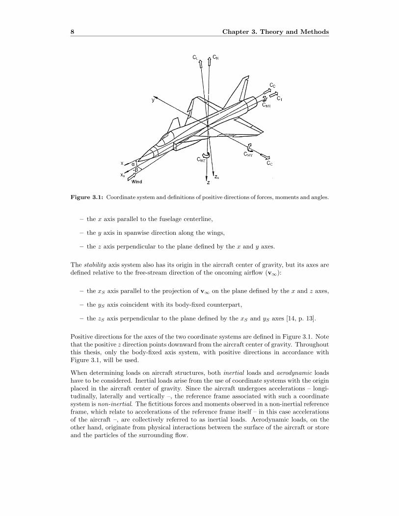
Figure 3.1: Coordinate system and definitions of positive directions of forces, moments and angles.
– the x axis parallel to the fuselage centerline,
– the y axis in spanwise direction along the wings,
– the z axis perpendicular to the plane defined by the x and y axes.
The stability axis system also has its origin in the aircraft center of gravity, but its axes aredefined relative to the free-stream direction of the oncoming airflow (v∞):
– the xS axis parallel to the projection of v∞ on the plane defined by the x and z axes,
– the yS axis coincident with its body-fixed counterpart,
– the zS axis perpendicular to the plane defined by the xS and yS axes [14, p. 13].
Positive directions for the axes of the two coordinate systems are defined in Figure 3.1. Notethat the positive z direction points downward from the aircraft center of gravity. Throughoutthis thesis, only the body-fixed axis system, with positive directions in accordance withFigure 3.1, will be used.
When determining loads on aircraft structures, both inertial loads and aerodynamic loadshave to be considered. Inertial loads arise from the use of coordinate systems with the originplaced in the aircraft center of gravity. Since the aircraft undergoes accelerations – longi-tudinally, laterally and vertically –, the reference frame associated with such a coordinatesystem is non-inertial. The fictitious forces and moments observed in a non-inertial referenceframe, which relate to accelerations of the reference frame itself – in this case accelerationsof the aircraft –, are collectively referred to as inertial loads. Aerodynamic loads, on theother hand, originate from physical interactions between the surface of the aircraft or storeand the particles of the surrounding flow.
3.1. Definitions 9
Throughout this thesis, only aerodynamic loads are considered. Any mention of loads refersto purely aerodynamic loads. Unless otherwise stated, the term loads is also considered toinclude both forces and moments on the store in question.
Aerodynamic forces and moments are generally described in terms of their components alongor about the coordinate axes. In the body-fixed axis system:
– the force components are denoted T for tangential force, C for side force and N fornormal force;
– the moment coefficients are denoted MX for rolling moment, MY for pitching momentand MZ for yawing moment.
Due to convention, positive loads do not necessarily have the same direction as the unitvectors of the coordinate system. Following standard flight mechanics conventions yieldsthe following equations for an arbitrary force (F) and moment (M) [14, p. 13]:
F = T (−x) + C(−y) +N(−z)
M = MX x+MY y +MZ z.(3.1)
In fluid dynamics, dimensionless parameters – such as the Mach number (M), the Reynoldsnumber (Re) and the Strouhal number (Sr) – are important in characterizing flows. Simi-larly, it is customary in aerodynamics to express loads as dimensionless aerodynamic coeffi-cients, which allow for comparison of aerodynamic properties for different length and velocityscales as well as in gases of different density. Each force and moment has its correspondingaerodynamic coefficient, with positive direction according to Figure 3.1:
– the tangential force coefficient (CT ), corresponding to T , the side force coefficient(CC), corresponding to C, and the normal force coefficient (CN ), corresponding to N ;
– the rolling moment coefficient (CMX), corresponding to MX , the pitching momentcoefficient (CMY ), corresponding to MY , and the yawing moment coefficient (CMZ),corresponding to MZ .
The relation between an arbitrary aerodynamic force coefficient (Ci) and the aerodynamicforce component (Fi) acting in the same direction as Ci, can be expressed as
Ci = Fi2
Srefρ∞ �v∞�2, (3.2)
where the reference area (Sref) of external stores is normally chosen as the cross-sectionalarea of the store body. Correspondingly, for an arbitrary aerodynamic moment coefficient(CMi) and its aerodynamic moment (Mi), one can state [1, pp. 20–21]
CMi = Mi2
crefSrefρ∞ �v∞�2, (3.3)
where the choice of reference length (cref) depends on which moment is considered – rolling,pitching or yawing.
10 Chapter 3. Theory and Methods
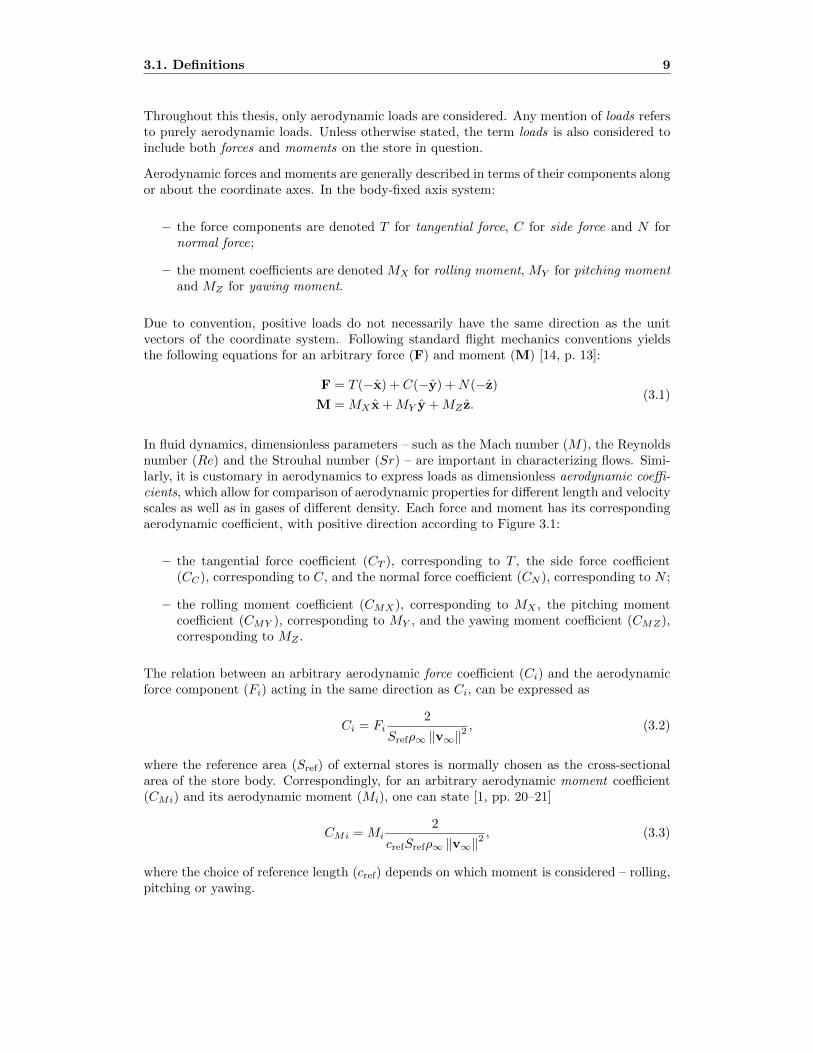
Figure 3.2: The main steps in the work process of the investigated scaling methodology.
Throughout this thesis, aerodynamic coefficients are consistently used to describe forcesand moments. Hence, the term loads should generally be interpreted as referring to thesecoefficients rather than to actual forces and moments. In addition, CT is normally notsubject to scaling and should therefore generally not be considered when references aremade to loads in this thesis.
3.2 Principles and Theory of the Scaling Methodology
The scaling method under investigation in this thesis, as proposed by C. Spjutare [25],consists of four main steps:
– modeling, in which the geometries of the reference and non-tested store configurationsare created;
– preprocessing, in which the computational mesh is created and prepared for simulationand input files, which contain relevant information for the simulation, are created;
– simulation, in which the flow solver Edge is executed and computes a solution to theEuler equations based on the computational mesh and the input files;
– post-processing, in which the simulation data are extracted, the ∆-effect is calculatedand the loads for the non-tested store are estimated by adding the ∆-effect to thewind tunnel data for the reference store.
In order to ensure mesh independence – i.e. that the solution is independent of the specificmesh used in the simulation – the preprocessing, simulation and post-processing steps canbe repeated with a different mesh size. Figure 3.2 provides an illustration of the workflowoutlined above, including an iteration for investigating mesh independence of the solution.
3.2.1 Modeling
The geometric modeling is performed in the surface modeling software sumo [7]. The basicbuilding objects of the sumo models are bodies and wings. Each model may consist of anarbitrary number of such objects. The user also has the option to define parts of objects asinflow and outflow regions – e.g. for a jet engine – or control surfaces – such as rudders andflaps. Such definitions will affect the computational mesh, described in section 3.2.2.
3.2. Principles and Theory of the Scaling Methodology 11
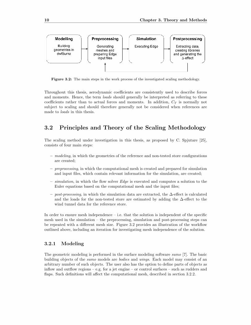
Figure 3.3: Modeling in sumo: the positioning of a store in an integrated model consisting ofaircraft, pylons and stores.
Bodies are three-dimensional objects of almost arbitrary shape, the only restriction beingthat they must be symmetrical along the y axis. Bodies are defined by specifying points atthe body surface at a series of cross-sections. The software connects the cross-sections usinginterpolation, thereby creating a continuous body surface. Wings are defined by specifyingthe position of the leading edge, the chord length and the airfoil shape at the wing root,at the wing tip and, if necessary, at additional span-wise sections of the wing. The airfoilcan be selected from a library of predefined profiles – such as various NACA profiles –,defined as a plate with a rounded leading edge or defined by loading an ASCII file of airfoilcoordinates. The surfaces between the defined sections are created by interpolation [7].
The aircraft and each pylon and/or store may be modeled separately. The pylon and storemodels may then be loaded into an integrated aircraft model and moved to the correctposition by supplying their coordinates in the aircraft coordinate system. Figure 3.3 showsthe positioning of a store being integrated into a model that already contains the aircraftand its pylons. The possibility of such integration of models provides a simple, and relativelyquick, means of creating models that reflect different store configurations for the aircraft.
3.2.2 Preprocessing
The surface mesh for the finished, integrated model is obtained using the built-in meshingfeatures of sumo. The unstructured mesh is generated automatically, based on the geome-tries of the supplied model and a number of user-defined parameters. Of these parameters,which can be set separately for each surface – body, wing, inflow/outflow region or controlsurface – in the model, the most prominent are the definitions of maximum and minimumelement edge length. These allow the user to choose which surfaces should be resolved ingreater detail and which should be resolved in less detail.
For each surface, the software provides a default setting for each parameter, based on geomet-ric properties such as curvature. The mesh is automatically adapted near the intersections
12 Chapter 3. Theory and Methods
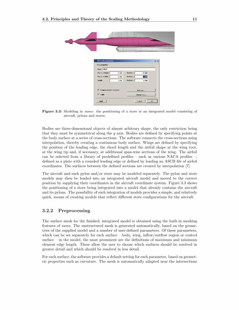
Figure 3.4: Mesh generation in sumo: surface mesh of a store and a pylon, with a dialog foradjusting mesh parameters.
of different surfaces, in order to obtain a complete, closed mesh. Additionally, the mesh isautomatically refined in regions of strong curvature, especially along the leading and trailingedges of wings [7]. Figure 3.4 shows a surface mesh of a store, consisting of several surfaces,and a pylon. Below the mesh visualization, a dialog box for adjusting the mesh parametersof one of the surfaces of the model is shown.
For the scaling method in question, a fine mesh resolution is generally chosen on the sur-faces of the evaluated store and adjacent surfaces, while a gradual coarsening of the meshresolution can be applied for surfaces further away from the store [25].
The computational domain for the CFD simulations consists of the volume of air surroundingthe aircraft and the stores. Hence, an unstructured volume mesh is generated from thesurface mesh, using the built-in TetGen interface [23]. The tetrahedral mesh generatorTetGen uses an algorithm based on constrained Delaunay tetrahedralization (CDT) to obtaina volume mesh that conforms to this domain, which is bounded by the surface mesh and adistant farfield boundary. The latter is created by sumo upon calling TetGen. The farfieldboundary is spherical in shape, with a user-defined radius, which is composed of mesh points,or nodes, with a resolution defined by the user through a farfield refinement parameter.
The TetGen algorithm performs a Delaunay tetrahedralization followed by a series of correc-tive measures, forcing the mesh to conform to the computational domain, such as insertingand/or moving nodes and removing tetrahedra that appear outside the computational do-main. Finally, the algorithm increases the quality of the mesh by inserting additional nodes,based on Delaunay refinement [24].
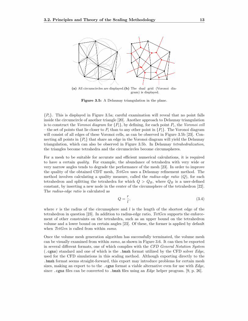
Delaunay tetrahedralization is the extension to three dimensions of the two-dimensional con-cept of Delaunay triangulation. Delaunay triangulation is the connection of a set of points{Pi} in a plane, to form triangles such that no circumcircle – the circle that passes throughthe three points from {Pi} that form the vertices of a triangle – contains any point from
3.2. Principles and Theory of the Scaling Methodology 13
(a) All circumcircles are displayed.(b) The dual grid (Voronoi dia-gram) is displayed.
Figure 3.5: A Delaunay triangulation in the plane.
{Pi}. This is displayed in Figure 3.5a; careful examination will reveal that no point fallsinside the circumcircle of another triangle [20]. Another approach to Delaunay triangulationis to construct the Voronoi diagram for {Pi}, by defining, for each point Pi, the Voronoi cell– the set of points that lie closer to Pi than to any other point in {Pi}. The Voronoi diagramwill consist of all edges of these Voronoi cells, as can be observed in Figure 3.5b [23]. Con-necting all points in {Pi} that share an edge in the Voronoi diagram will yield the Delaunaytriangulation, which can also be observed in Figure 3.5b. In Delaunay tetrahedralization,the triangles become tetrahedra and the circumcircles become circumspheres.
For a mesh to be suitable for accurate and efficient numerical calculations, it is requiredto have a certain quality. For example, the abundance of tetrahedra with very wide orvery narrow angles tends to degrade the performance of the mesh [23]. In order to improvethe quality of the obtained CDT mesh, TetGen uses a Delaunay refinement method. Themethod involves calculating a quality measure, called the radius-edge ratio (Q), for eachtetrahedron and splitting the tetrahedra for which Q > QB , where QB is a user-definedconstant, by inserting a new node in the center of the circumsphere of the tetrahedron [22].The radius-edge ratio is calculated as
Q =r
l, (3.4)
where r is the radius of the circumsphere and l is the length of the shortest edge of thetetrahedron in question [23]. In addition to radius-edge ratio, TetGen supports the enforce-ment of other constraints on the tetrahedra, such as an upper bound on the tetrahedronvolume and a lower bound on certain angles [23]. Of these, the former is applied by defaultwhen TetGen is called from within sumo.
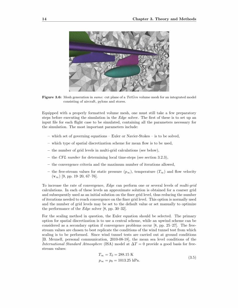
Once the volume mesh generation algorithm has successfully terminated, the volume meshcan be visually examined from within sumo, as shown in Figure 3.6. It can then be exportedin several different formats, one of which complies with the CFD General Notation System(.cgns) standard and one of which is the .bmsh format utilized by the CFD solver Edge,used for the CFD simulations in this scaling method. Although exporting directly to the.bmsh format seems straight-forward, this export may introduce problems for certain meshsizes, making an export to to the .cgns format a viable alternative even for use with Edge,since .cgns files can be converted to .bmsh files using an Edge helper program. [9, p. 26].
14 Chapter 3. Theory and Methods
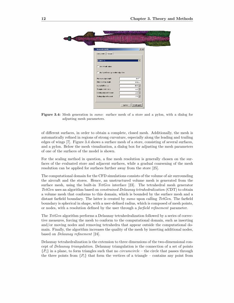
Figure 3.6: Mesh generation in sumo: cut plane of a TetGen volume mesh for an integrated modelconsisting of aircraft, pylons and stores.
Equipped with a properly formatted volume mesh, one must still take a few preparatorysteps before executing the simulation in the Edge solver. The first of these is to set up aninput file for each flight case to be simulated, containing all the parameters necessary forthe simulation. The most important parameters include:
– which set of governing equations – Euler or Navier-Stokes – is to be solved,
– which type of spatial discretization scheme for mean flow is to be used,
– the number of grid levels in multi-grid calculations (see below),
– the CFL number for determining local time-steps (see section 3.2.3),
– the convergence criteria and the maximum number of iterations allowed,
– the free-stream values for static pressure (p∞), temperature (T∞) and flow velocity(v∞) [9, pp. 19–20, 67–76].
To increase the rate of convergence, Edge can perform one or several levels of multi-gridcalculations. In each of these levels an approximate solution is obtained for a coarser gridand subsequently used as an initial solution on the finer grid level, thus reducing the numberof iterations needed to reach convergence on the finer grid level. This option is normally usedand the number of grid levels may be set to the default value or set manually to optimizethe performance of the Edge solver [8, pp. 30–32].
For the scaling method in question, the Euler equation should be selected. The primaryoption for spatial discretization is to use a central scheme, while an upwind scheme can beconsidered as a secondary option if convergence problems occur [8, pp. 25–27]. The free-stream values are chosen to best replicate the conditions of the wind tunnel test from whichscaling is to be performed. Since wind tunnel tests are carried out at ground conditions[B. Mexnell, personal communication, 2010-08-18], the mean sea level conditions of theInternational Standard Atmosphere (ISA) model at ∆T = 0 provide a good basis for free-stream values:
T∞ = T0 = 288.15 K
p∞ = p0 = 1013.25 hPa.(3.5)
3.2. Principles and Theory of the Scaling Methodology 15
The free-stream flow velocity vector is calculated for each case to be simulated, usingcorresponding values for M , α and β and the ISA mean sea level speed of sound (a0 =340.29 m/s), as:
v∞ = Ma0
�− cos (α) cos (β)x− sin (β)y + sin (α) cos (β)z
�, (3.6)
where unit vectors are defined according to Figure 3.1.
Other input parameters may be set to default values or set manually to optimize the per-formance of the Edge solver. However, it is advisable to use the same or similar settingsfor all flight cases and for both configurations involved in scaling, unless computationalconsiderations require otherwise.
The second preparatory step is to specify boundary conditions for the farfield and theinternal boundaries, consisting of all surfaces of the supplied model. Edge offers a total of23 different types of boundary conditions, most of which are related to inflow and outflowboundaries [9, pp. 20, 41–46]. For all solid surfaces of the aircraft, pylons and stores, theEuler wall boundary condition should be selected, while the farfield boundary should havethe Farfield boundary condition selected. For other inflow and outflow boundaries, such asengine intakes and nozzles, the choice of boundary conditions depends on what data areavailable for these boundaries. The Weak static pressure, Weak total states, Mass flow inletand Mass flow outlet are potential candidates at such boundaries. If no engine data areavailable, an approximation of the flow through such boundaries can be made by using theFarfield boundary condition [P. Weinerfelt, personal communication, 2010-10-15].
The final preparatory step is to run the Edge preprocessor. The preprocessor discretizes thecomputational domain by constructing control volumes for each node in the volume meshand defines the control surfaces – the interfaces between these control volumes. The controlvolumes are formed by the dual grid of the volume mesh [8, pp. 9–11]. As the dual gridconsists of the Voronoi diagram of the nodes [23], each control volume coincides with theVoronoi cell of the node in question. If the input file indicates that multi-grid calculationsare to be performed, the preprocessor will generate the coarser grids for such simulations byagglomeration of control volumes from finer grid levels. In addition, the preprocessor willpartition the grid for parallel computations on multiple processors [9, p. 21].
3.2.3 Simulation
Upon completion of the preprocessor run, simulations may be initiated by executing theEdge solver. The flow solver will seek a numerical solution to the set of governing equationsselected, using the information from the mesh, the input files, the boundary conditions andthe results of the preprocessor run. Each flight case requires a separate simulation. However,when executed on a computer cluster, all simulations can be run simultaneously.
A full description of the mechanics of the flow solver is extensive and the interested readeris referred to the Edge documentation [8]. Here, a few key concepts relating to solving theEuler equation for a calorically perfect gas using a central scheme are addressed briefly. Asimilar description can be made for the upwind schemes, which rely on Roe flux differencesplitting [8, pp. 27–29], but this is omitted due to the lower priority of such schemes as partof this scaling method.
16 Chapter 3. Theory and Methods
The Euler equations relate the conservative solution vector (U) to the flux tensor (FI) andthe source vector (Q) [8, p. 12]. They can be expressed in vector form as
∂U
∂t+∇ · FI = Q, (3.7)
whereFI = fI1 x+ fI2 y + fI3 z (3.8)
The conservative solution vector and the flux vectors (fIi) are given as
U =
ρ
ρv1
ρv2
ρv3
ρE
, fIi =
ρvi
pδ1i + ρviv1
pδ2i + ρviv2
pδ3i + ρviv3
(p+ ρE)vi
, (3.9)
where i ∈ {1, 2, 3} denote the x, y and z directions, respectively, and E is the total energy– internal and kinetic – of the gas [2, pp. 77–78].
The static pressure (p) needed to solve the above equations is obtained from the equationof state for the gas model selected for the simulation. For a calorically perfect gas, which isa common assumption in aerodynamics [8, p. 15], the equations of state yield
p = (γ − 1)
�ρE − �ρv�2
2ρ
�. (3.10)
If (3.7) is applied to a finite volume, e.g. the control volume for node ν0, one obtains
∂
∂t(U0V0) +
m0�
k=1
FI0kn0kS0k = Q0V0, (3.11)
where the summation is taken over the m0 neighbors of the node, and n0k is the normalizednormal vector for the surface S0k, separating the control volume of node ν0 from the controlvolume of its neighbor node νk [8, pp. 10, 25].
The flux matrices (FI0k) in (3.11) are those described in (3.8) and (3.9), but the solutionvectors used to calculate their values depend on the discretization scheme used. For thecentral scheme, the inviscid flux is calculated using the average of the values for the twonodes involved, as shown in
FI0k = FI
�U0 +Uk
2
�− d0k. (3.12)
Here, d0k denotes artificial dissipation, which is added to improve the numerical stabilityof the solution. The amount of artificial dissipation added is controlled by the user throughtwo constants – the second and fourth order dissipation coefficients (κ(2) and κ
(4)) –, bothof which are defined as input parameters to the Edge solver [8, p. 26].
For solving (3.11) numerically, an explicit multistage Runge-Kutta scheme is used. If theequation is written on the general form
dU
dt= f(U), (3.13)
3.2. Principles and Theory of the Scaling Methodology 17
the q-stage Runge-Kutta scheme can be written
u(1) = u
n + α1∆tf(un)
u(2) = u
n + α2∆tf(u(1))
...
u(q) = u
n + αq∆tf(u(q−1))
un+1 = u
(q),
(3.14)
where the coefficients αi are defined by the user in the input file. The default setting isa 3-stage scheme, with coefficients that generally provide good stability of the solution [8,pp. 32–33]. The local time-stepping feature of Edge steady-state calculations implies thatthe time-step (∆t) in (3.14) is determined locally for each node ν0. For inviscid flow this iscalculated according to
∆t0 = CFLV0
λ0, (3.15)
where λ0 is the integrated spectral radius of the node, which increases with increasing flowvelocity and increasing speed of sound [8, pp. 26, 32–33]. This implies that longer time-steps will be used at nodes for which less fluid passes through its control volume per unittime, resulting in a more efficient use of computing resources. The CFL parameter is theuser-defined CFL number, deeply related to the Courant-Friedrichs-Lewy (CFL) conditionfor convergence of numerical solutions of certain PDEs, which provides an upper limit onthe time-step for numerical schemes solving such PDEs [5].
The calculations outlined above are continued until the user-defined convergence criteriaare satisfied, the maximum number of iterations is reached or the solution diverges. In thecase of divergence, the simulation must be rerun, with changes either in the parameters ofthe input file or in the geometry of the mesh. Potential input parameter changes includelowering the CFL number – to obtain shorter local time-steps –, increasing the amountof artificial dissipation – to obtain a better smoothing of the solution – and/or switchingdiscretization scheme to an upwind scheme [9, p. 39].
Solutions with very slow convergence, or non-convergent solutions that neither reach theconvergence criterion nor diverge, may be used for scaling if they appear well-behaved uponinspection of residuals and flow field during post-processing (see section 3.2.4) [E. Amunds-son, personal communication, 2010-10-07].
3.2.4 Post-Processing
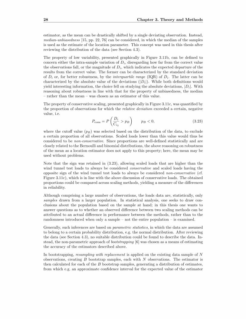
When the simulations have reached convergent, or at least satisfying non-divergent, solu-tions, the post-processing step follows. Initially, the solutions must be inspected to deter-mine whether the results can be assumed to be reliable. This is particularly important ifthe convergence criteria were not met. The first source for information about convergencerate etc. is the residual output file, to which the Edge solver regularly writes residual dataduring the solution process. This allows the user to assess global convergence by monitoringthe magnitude of the residuals and the integrated values of forces and moments as functionsof iteration number for the entire mesh [9, p. 33].
18 Chapter 3. Theory and Methods
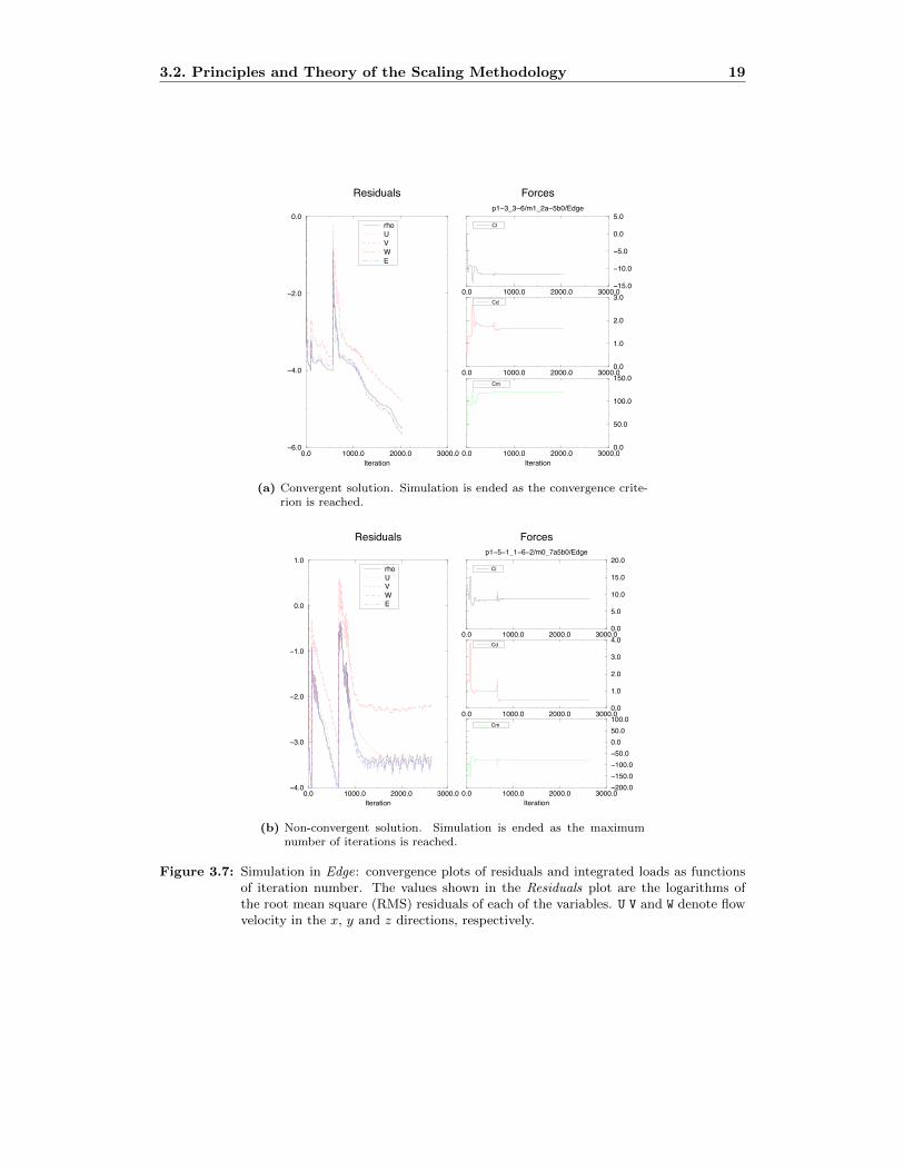
Figure 3.7 shows two plots of the contents of this file, one for a convergent solution (3.7a)and one for a non-convergent solution (3.7b). In the plots, one can also observe severaldisjoint intervals in the generally decreasing residuals, separated by a sudden increase invalue of the residuals. This indicates a transition from a coarser to a finer grid in a multi-grid simulation. The simulations yielding the plots in Figure 3.7 were multi-grid simulationswith three grid levels, which is consistent with the three intervals observed in the plots.
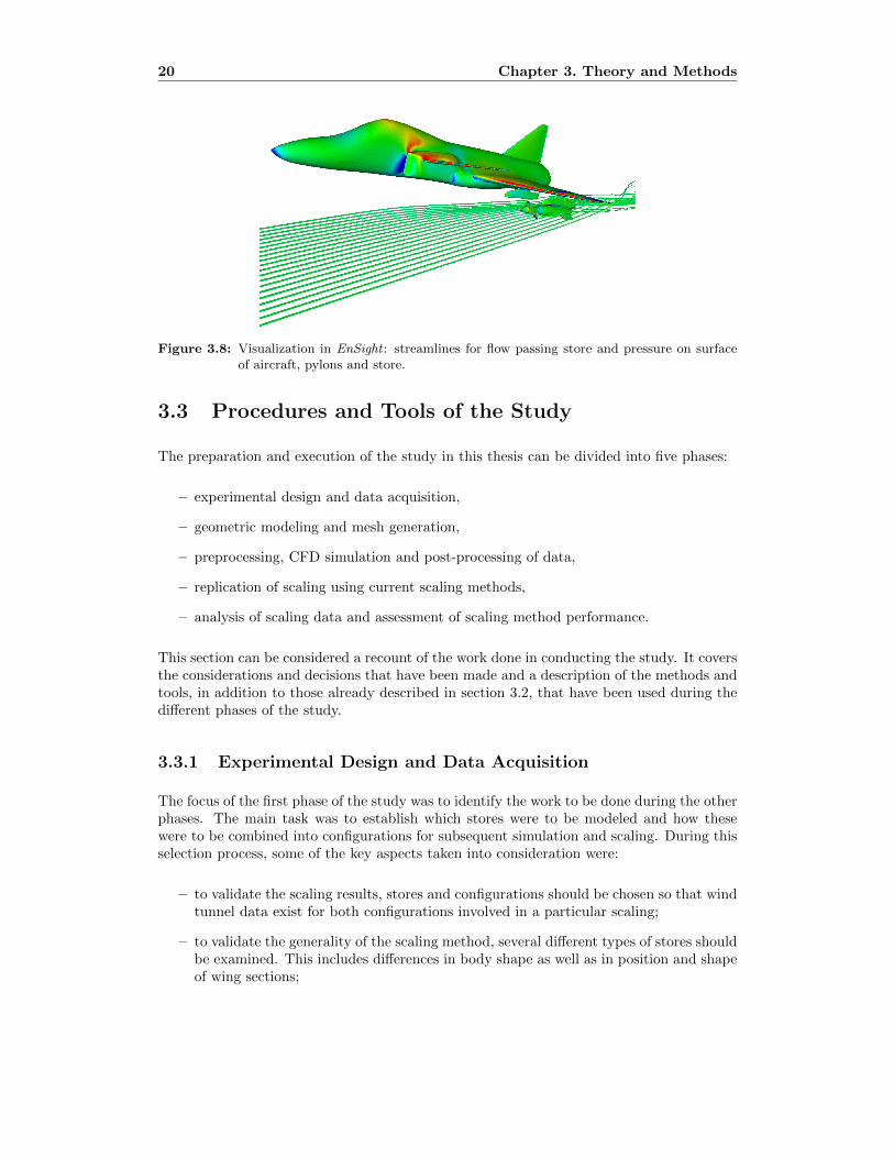
Although the integrated loads globally converge to a value, which can be seen e.g. for bothcases in Figure 3.7, local fluctuations may occur, yielding unreliable results when loads onsmaller parts of the model, such as stores, are considered. Therefore, the solution should alsobe inspected in a flow visualization program. Using an Edge helper program, the solutionmay be exported to a format readable by the flow visualization tool EnSight [9, p. 23].
In EnSight, the flow field may be inspected visually using a wide range of tools, such ascontour plots, cut planes and streamlines, and the values of variables on surfaces may bevisually inspected using coloring, elevated surfaces etc. One of the indications of a non-reliable solution is the existence of unexpectedly large local pressure gradients, particularlywhere such gradients are not expected [E. Amundsson, personal communication, 2010-10-07]. Generally, the visual inspection of the solution demands more of the user, in terms ofknowledge of aerodynamics, than the inspection of global convergence by monitoring theresiduals. A visualization in EnSight is shown in Figure 3.8.
If the simulation results are deemed reliable, the next step is to calculate the aerodynamiccoefficients of the investigated store. As part of the output, Edge generates aerodynamiccoefficients for every surface in the model. The coefficients for the surfaces belonging to theinvestigated store are extracted and summed, to generate the aerodynamic coefficients ofthe entire store for the flight case in question:
Ci,store =n�
k=1
Ci,k, (3.16)
where Ci is any aerodynamic coefficient and n is the number of surfaces of the store. Thisextraction and summation is repeated for all coefficients and all flight cases for simulationsof both the reference and the non-tested store.
The final step of the post-processing is to calculate the ∆-effect and perform the actualscaling of the loads between the two stores. If Ci1,CFD is an aerodynamic coefficient for thereference store obtained by simulation and Ci2,CFD is the corresponding coefficient for thenon-tested store, the ∆-effect is simply
∆Ci,CFD = Ci2,CFD − Ci1,CFD. (3.17)
Given the ∆-effect and the wind tunnel data for the reference store, the actual coefficientsof the non-tested store can be estimated by scaling, using the simple relation
Ci2 = Ci1 +∆Ci,CFD, (3.18)
where Ci1 is the aerodynamic coefficient for the reference store obtained by wind tunneltests and Ci2 is the estimate of the corresponding coefficient for the non-tested store.
3.2. Principles and Theory of the Scaling Methodology 19
0.0 1000.0 2000.0 3000.0Iteration
−6.0
−4.0
−2.0
0.0
Residuals
rhoUVWE
0.0 1000.0 2000.0 3000.0−15.0
−10.0
−5.0
0.0
5.0
Forcesp1−3_3−6/m1_2a−5b0/Edge
Cl
0.0 1000.0 2000.0 3000.00.0
1.0
2.0
3.0Cd
0.0 1000.0 2000.0 3000.0Iteration
0.0
50.0
100.0
150.0Cm
(a) Convergent solution. Simulation is ended as the convergence crite-rion is reached.
0.0 1000.0 2000.0 3000.0Iteration
−4.0
−3.0
−2.0
−1.0
0.0
1.0
Residuals
rhoUVWE
0.0 1000.0 2000.0 3000.00.0
5.0
10.0
15.0
20.0
Forcesp1−5−1_1−6−2/m0_7a5b0/Edge
Cl
0.0 1000.0 2000.0 3000.00.0
1.0
2.0
3.0
4.0Cd
0.0 1000.0 2000.0 3000.0Iteration
−200.0−150.0−100.0−50.00.050.0100.0
Cm
(b) Non-convergent solution. Simulation is ended as the maximumnumber of iterations is reached.
Figure 3.7: Simulation in Edge: convergence plots of residuals and integrated loads as functionsof iteration number. The values shown in the Residuals plot are the logarithms ofthe root mean square (RMS) residuals of each of the variables. U V and W denote flowvelocity in the x, y and z directions, respectively.
20 Chapter 3. Theory and Methods
Figure 3.8: Visualization in EnSight : streamlines for flow passing store and pressure on surfaceof aircraft, pylons and store.
3.3 Procedures and Tools of the Study
The preparation and execution of the study in this thesis can be divided into five phases:
– experimental design and data acquisition,
– geometric modeling and mesh generation,
– preprocessing, CFD simulation and post-processing of data,
– replication of scaling using current scaling methods,
– analysis of scaling data and assessment of scaling method performance.
This section can be considered a recount of the work done in conducting the study. It coversthe considerations and decisions that have been made and a description of the methods andtools, in addition to those already described in section 3.2, that have been used during thedifferent phases of the study.
3.3.1 Experimental Design and Data Acquisition
The focus of the first phase of the study was to identify the work to be done during the otherphases. The main task was to establish which stores were to be modeled and how thesewere to be combined into configurations for subsequent simulation and scaling. During thisselection process, some of the key aspects taken into consideration were:
– to validate the scaling results, stores and configurations should be chosen so that windtunnel data exist for both configurations involved in a particular scaling;
– to validate the generality of the scaling method, several different types of stores shouldbe examined. This includes differences in body shape as well as in position and shapeof wing sections;
3.3. Procedures and Tools of the Study 21
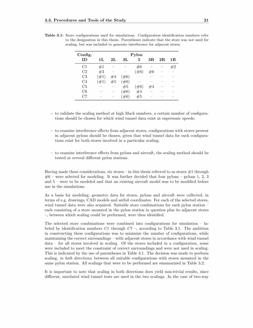
Table 3.1: Store configurations used for simulations. Configuration identification numbers referto the designation in this thesis. Parentheses indicate that the store was not used forscaling, but was included to generate interference for adjacent stores.
Config. Pylon
ID 1L 2L 3L 5 3R 2R 1R
C1 #1 – – #6 – – #2C2 #3 – – (#6) #6 – –C3 (#1) #4 (#6) – – – –C4 (#1) #5 (#6) – – – –C5 – – #5 (#6) #4 – –C6 – – (#6) #4 – – –C7 – – (#6) #5 – – –
– to validate the scaling method at high Mach numbers, a certain number of configura-tions should be chosen for which wind tunnel data exist at supersonic speeds;
– to examine interference effects from adjacent stores, configurations with stores presentin adjacent pylons should be chosen, given that wind tunnel data for such configura-tions exist for both stores involved in a particular scaling;
– to examine interference effects from pylons and aircraft, the scaling method should betested at several different pylon stations.
Having made these considerations, six stores – in this thesis referred to as stores #1 through#6 – were selected for modeling. It was further decided that four pylons – pylons 1, 2, 3and 5 – were to be modeled and that an existing aircraft model was to be modified beforeuse in the simulations.
As a basis for modeling, geometry data for stores, pylons and aircraft were collected, interms of e.g. drawings, CAD models and airfoil coordinates. For each of the selected stores,wind tunnel data were also acquired. Suitable store combinations for each pylon station –each consisting of a store mounted in the pylon station in question plus its adjacent stores–, between which scaling could be performed, were then identified.
The selected store combinations were combined into configurations for simulation – la-beled by identification numbers C1 through C7 –, according to Table 3.1. The ambitionin constructing these configurations was to minimize the number of configurations, whilemaintaining the correct surroundings – with adjacent stores in accordance with wind tunneldata – for all stores involved in scaling. Of the stores included in a configuration, somewere included to meet the constraint of correct surroundings and were not used in scaling.This is indicated by the use of parentheses in Table 3.1. The decision was made to performscaling, in both directions, between all suitable configurations with stores mounted in thesame pylon station. All scalings that were to be performed are summarized in Table 3.2.
It is important to note that scaling in both directions does yield non-trivial results, sincedifferent, unrelated wind tunnel tests are used in the two scalings. In the case of two-way
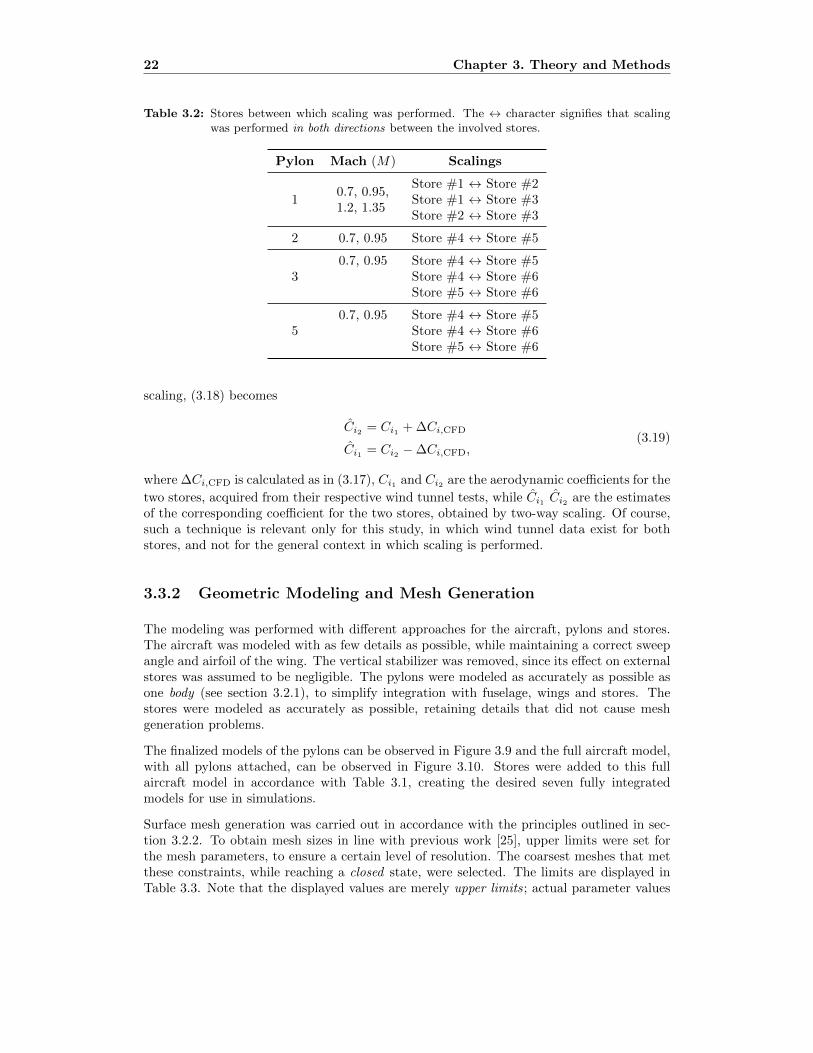
22 Chapter 3. Theory and Methods
Table 3.2: Stores between which scaling was performed. The ↔ character signifies that scalingwas performed in both directions between the involved stores.
Pylon Mach (M) Scalings
10.7, 0.95,1.2, 1.35
Store #1 ↔ Store #2Store #1 ↔ Store #3Store #2 ↔ Store #3
2 0.7, 0.95 Store #4 ↔ Store #5
30.7, 0.95 Store #4 ↔ Store #5
Store #4 ↔ Store #6Store #5 ↔ Store #6
50.7, 0.95 Store #4 ↔ Store #5
Store #4 ↔ Store #6Store #5 ↔ Store #6
scaling, (3.18) becomes
Ci2 = Ci1 +∆Ci,CFD
Ci1 = Ci2 −∆Ci,CFD,(3.19)
where∆Ci,CFD is calculated as in (3.17), Ci1 and Ci2 are the aerodynamic coefficients for the
two stores, acquired from their respective wind tunnel tests, while Ci1 Ci2 are the estimatesof the corresponding coefficient for the two stores, obtained by two-way scaling. Of course,such a technique is relevant only for this study, in which wind tunnel data exist for bothstores, and not for the general context in which scaling is performed.
3.3.2 Geometric Modeling and Mesh Generation
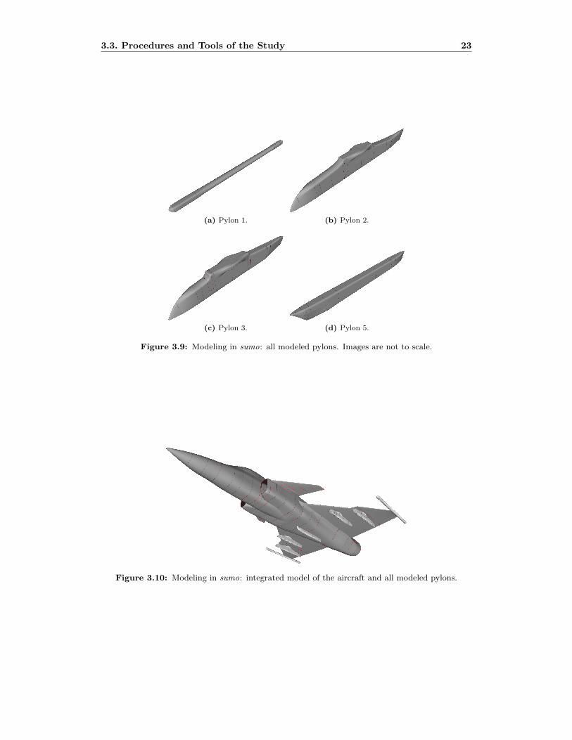
The modeling was performed with different approaches for the aircraft, pylons and stores.The aircraft was modeled with as few details as possible, while maintaining a correct sweepangle and airfoil of the wing. The vertical stabilizer was removed, since its effect on externalstores was assumed to be negligible. The pylons were modeled as accurately as possible asone body (see section 3.2.1), to simplify integration with fuselage, wings and stores. Thestores were modeled as accurately as possible, retaining details that did not cause meshgeneration problems.
The finalized models of the pylons can be observed in Figure 3.9 and the full aircraft model,with all pylons attached, can be observed in Figure 3.10. Stores were added to this fullaircraft model in accordance with Table 3.1, creating the desired seven fully integratedmodels for use in simulations.
Surface mesh generation was carried out in accordance with the principles outlined in sec-tion 3.2.2. To obtain mesh sizes in line with previous work [25], upper limits were set forthe mesh parameters, to ensure a certain level of resolution. The coarsest meshes that metthese constraints, while reaching a closed state, were selected. The limits are displayed inTable 3.3. Note that the displayed values are merely upper limits ; actual parameter values
3.3. Procedures and Tools of the Study 23
(a) Pylon 1. (b) Pylon 2.
(c) Pylon 3. (d) Pylon 5.
Figure 3.9: Modeling in sumo: all modeled pylons. Images are not to scale.
Figure 3.10: Modeling in sumo: integrated model of the aircraft and all modeled pylons.
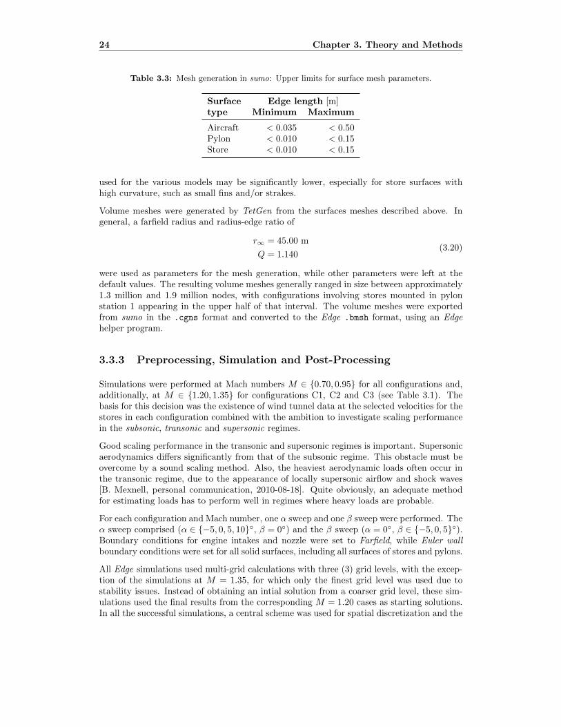
24 Chapter 3. Theory and Methods
Table 3.3: Mesh generation in sumo: Upper limits for surface mesh parameters.
Surface Edge length [m]type Minimum Maximum
Aircraft < 0.035 < 0.50Pylon < 0.010 < 0.15Store < 0.010 < 0.15
used for the various models may be significantly lower, especially for store surfaces withhigh curvature, such as small fins and/or strakes.
Volume meshes were generated by TetGen from the surfaces meshes described above. Ingeneral, a farfield radius and radius-edge ratio of
r∞ = 45.00 m
Q = 1.140(3.20)
were used as parameters for the mesh generation, while other parameters were left at thedefault values. The resulting volume meshes generally ranged in size between approximately1.3 million and 1.9 million nodes, with configurations involving stores mounted in pylonstation 1 appearing in the upper half of that interval. The volume meshes were exportedfrom sumo in the .cgns format and converted to the Edge .bmsh format, using an Edgehelper program.
3.3.3 Preprocessing, Simulation and Post-Processing
Simulations were performed at Mach numbers M ∈ {0.70, 0.95} for all configurations and,additionally, at M ∈ {1.20, 1.35} for configurations C1, C2 and C3 (see Table 3.1). Thebasis for this decision was the existence of wind tunnel data at the selected velocities for thestores in each configuration combined with the ambition to investigate scaling performancein the subsonic, transonic and supersonic regimes.
Good scaling performance in the transonic and supersonic regimes is important. Supersonicaerodynamics differs significantly from that of the subsonic regime. This obstacle must beovercome by a sound scaling method. Also, the heaviest aerodynamic loads often occur inthe transonic regime, due to the appearance of locally supersonic airflow and shock waves[B. Mexnell, personal communication, 2010-08-18]. Quite obviously, an adequate methodfor estimating loads has to perform well in regimes where heavy loads are probable.
For each configuration and Mach number, one α sweep and one β sweep were performed. Theα sweep comprised (α ∈ {−5, 0, 5, 10}◦, β = 0◦) and the β sweep (α = 0◦, β ∈ {−5, 0, 5}◦).Boundary conditions for engine intakes and nozzle were set to Farfield, while Euler wallboundary conditions were set for all solid surfaces, including all surfaces of stores and pylons.
All Edge simulations used multi-grid calculations with three (3) grid levels, with the excep-tion of the simulations at M = 1.35, for which only the finest grid level was used due tostability issues. Instead of obtaining an intial solution from a coarser grid level, these sim-ulations used the final results from the corresponding M = 1.20 cases as starting solutions.In all the successful simulations, a central scheme was used for spatial discretization and the
3.3. Procedures and Tools of the Study 25
coefficients of the three-stage Runge-Kutta method used were left at the default values. Forthe supersonic flight cases, the CFL number was lowered – from CFL = 0.90 to CFL = 0.60and the amount of artificial dissipation was increased – from (κ(2)
,κ(4)) = (0.50, 0.03) to
(κ(2),κ
(4)) = (1.00, 0.05) – compared to the subsonic and transonic simulations.
All grids were partitioned and the simulations were run using parallel computations, utilizingeight (8) processor cores per simulation, on the Linux-based Skylord/Darkstar cluster at theNational Supercomputer Centre (NSC) in Linkoping, Sweden [19].
Store loads were extracted from the simulation results, in accordance with (3.16), and werecompiled, sweep by sweep, for each store, pylon station and Mach number combination.Scaling was then performed in accordance with Table 3.2. The obtained scaled aerodynamiccoefficients, corresponding to a total of 104 sweeps, were saved and used to assess scalingmethod performance in the last phase of the study.
3.3.4 Scaling with Current Methods
The purpose of this study is to examine to what extent the proposed scaling method providesa higher degree of accuracy, generality and flexibility than the scaling methods currentlyin use. The performance of the method is thus assessed in relation to the current scalingmethods. This implies that all scalings should be repeated using the current scaling methodsand the results should be compared to those obtained using the proposed scaling method.This requires knowledge of the current scaling methods and an ability to straightforwardlyperform scaling using these methods.
As stated in Section 2.3.1, there are two methods currently in use for scaling aerodynamicloads on external stores, within this thesis referred to as the Louw and skal methods,respectively. During this phase of the study, the two scaling methods were examined –by digestion of available documentation and source code –, and scripts for performing thescaling using these methods were constructed.
Scaling was performed with both the Louw and skal methods, for all the 104 sweeps forwhich data existed for the investigated scaling method. Since the raw CFD data from thesimulations were readily available, estimating the loads directly by the coefficients obtainedfrom simulations was considered an alternate method, which was also evaluated.
For the Louw method, two different variants were considered. The main difference betweenthem is the assumption about which dimensions play a greater role in generating loads onthe store; the first variant emphasizes the dimensions of the store body, while the secondvariant gives greater weight to the dimensions of the fins and wing sections. Both variantswere included in the study.
For the skal method, two variants of the equations, differing in complexity, were consid-ered. Furthermore, another feature, for which two different options could be selected, wasidentified during the implementation of the scaling method. Both these options were alsoconsidered. Altogether, this resulted in four versions of the skal method, all of which wereevaluated.
26 Chapter 3. Theory and Methods
3.3.5 Data Analysis and Assessment of Method Performance
The investigation into the performance of the proposed scaling method in relation to thecurrent scaling methods is a non-trivial task, given the vast amount of data generated fromall the scalings using the various methods. In order to evaluate such a large data set,statistical analysis of the data was called for. This required, firstly, that one or severalstatistics, by which the quality of scaling results could be measured, were found. Secondly,it required statistical methods by which the values of these statistics could be interpretedand inferences be made about the performances of the scaling methods.
The first task was to identify the statistics by which performance could be measured. Threeproperties of the scaling results were identified as indications of sound scaling method. Thesewere:
– unbiased estimates, implying that values obtained through scaling, on average, can beexpected to coincide with the correct values obtained in wind tunnel tests,
– low variability, implying that the difference between the values obtained by scalingand the wind tunnel values generally can be expected to be small,
– conservative scaling, implying that values obtained by scaling generally can be ex-pected to not severely underestimate the correct values obtained in wind tunnel tests.
While the first two can be considered to be self-explanatory, the third property may re-quire further explanation. This property relates to the context of loads determination, inwhich the scaling method will be used. As the results of scaling will serve as basis forstress analyses, the underestimation of loads will lead to an underestimation of the stressesinduced in the store and the pylon-store interface. This may lead to dimensioning errorsor misconceptions about the operational capabilities of a particular aircraft configuration,which could jeopardize the safe operation of the aircraft. It is therefore vital that loads arenot underestimated. Additionally, loads having the correct magnitude but the wrong signmay lead to fundamentally different results in the stress analysis. Such loads cannot beconsidered conservative.
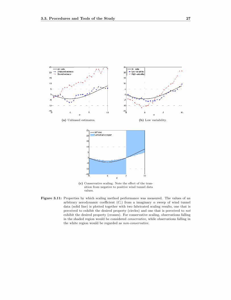
The properties are described in detail below, but the intuitive graphical representations ofthe properties are given in Figure 3.11. Central to all these properties is the deviation (Di)of the scaling results from the correct, wind tunnel test value. This is simply the difference
Di = Ci2 − Ci2 (3.21)
for an arbitrary aerodynamic coefficient and a specific flight case.
The property of unbiasedness, presented graphically in Figure 3.11a, relates to the actualvalue of Di. It can be statistically examined by hypothesis testing, with the tested hypothe-ses being
H0 : E[Di] = 0
H1 : E[Di] �= 0.(3.22)
However, for data which departs significantly from e.g. a normal distribution, the mean ofthe observations, which is normally used to determine bias, may not be a necessarily robust
3.3. Procedures and Tools of the Study 27
(a) Unbiased estimates. (b) Low variability.
(c) Conservative scaling. Note the effect of the tran-sition from negative to positive wind tunnel datavalues.
Figure 3.11: Properties by which scaling method performance was measured. The values of anarbitrary aerodynamic coefficient (Ci) from a imaginary α sweep of wind tunneldata (solid line) is plotted together with two fabricated scaling results, one that isperceived to exhibit the desired property (circles) and one that is perceived to notexhibit the desired property (crosses). For conservative scaling, observations fallingin the shaded region would be considered conservative, while observations falling inthe white region would be regarded as non-conservative.
28 Chapter 3. Theory and Methods
estimator, as the mean can be drastically shifted by a single deviating observation. Instead,median-unbiasedness [15, pp. 22, 76] can be considered, in which the median of the samplesis used as the estimate of the location parameter. This concept was used in this thesis afterreviewing the distribution of the data (see Section 4.3).
The property of low variability, presented graphically in Figure 3.11b, can be defined toconcern either the intra-sample variation of Di, disregarding how far from the correct valuethe observations fall, or the magnitude of Di, which indicates the expected departure of theresults from the correct value. The former can be characterized by the standard deviationof Di or, for better robustness, by the interquartile range (IQR) of Di. The latter can becharacterized by the absolute value of the deviations (|Di|). While both definitions wouldyield interesting information, the choice fell on studying the absolute deviations, |Di|. Withreasoning about robustness in line with that for the property of unbiasedness, the median– rather than the mean – was chosen as an estimator of this value.
The property of conservative scaling, presented graphically in Figure 3.11c, was quantified bythe proportion of observations for which the relative deviation exceeded a certain, negativevalue, i.e.
Pcons = P
�Di
Ci2
> pB
�pB < 0, (3.23)
where the cutoff value (pB) was selected based on the distribution of the data, to excludea certain proportion of all observations. Scaled loads lower than this value would thus beconsidered to be non-conservative. Since proportions are well-defined statistically and areclosely related to the Bernoulli and binomial distributions, the above reasoning on robustnessof the mean as a location estimator does not apply to this property; here, the mean may beused without problems.
Note that the sign was retained in (3.23), allowing scaled loads that are higher than thewind tunnel test loads to always be considered conservative and scaled loads having theopposite sign of the wind tunnel test loads to always be considered non-conservative (cf.Figure 3.11c), which is in line with the above discussion of conservative loads. The obtainedproportions could be compared across scaling methods, yielding a measure of the differencesin reliability.
Although comprising a large number of observations, the loads data are, statistically, onlysamples drawn from a larger population. In statistical analysis, one seeks to draw con-clusions about the population based on the sample at hand; in this thesis one wants toanswer questions as to whether an observed difference between two scaling methods can beattributed to an actual difference in performance between the methods, rather than to therandomness introduced when only a sample – not the entire population – is examined.
Generally, such inferences are based on parametric statistics, in which the data are assumedto belong to a certain probability distribution, e.g. the normal distribution. After reviewingthe data (see Section 4.3), no suitable distribution could be found to describe the data. In-stead, the non-parametric approach of bootstrapping [6] was chosen as a means of estimatingthe accuracy of the estimators described above.
In bootstrapping, resampling with replacement is applied on the existing data sample of Nobservations, creating B bootstrap samples, each with N observations. The estimator isthen calculated for each of the B bootstrap samples, generating a distribution of estimates,from which e.g. an approximate confidence interval for the expected value of the estimator
3.3. Procedures and Tools of the Study 29
can be calculated [6]. Comparison of these confidence intervals provides a means of makinginference about differences between the populations of the data.
However elegant, the bootstrapping approach described above is a univariate method, whichgives no information about how the scaling performance of a particular scaling method de-pends on variables such as M , α or β or on the types of stores involved in scaling. Suchinferences require the use of multivariate data analysis. Although non-parametric multivari-ate methods exist [3, 4, 10, 13], modeling many variables simultaneously may prove to bedifficult with such methods and, in addition, their statistical power – the ability to detect anactual difference between two groups – is often weak [26]. Hence, the parametric method ofn-way analysis of variance (ANOVA) was selected for the multivariate study, partly becauseof its ease of use compared to the referenced non-parametric methods. Although assumingnormal distribution of the data, ANOVA has been shown to be fairly robust to violationsof this assumption [12].
In n-way ANOVA, the response – in this case the value of e.g. Di – is related to n differenttreatments – values of variables such as M , α, β, target store etc. – through a linear modelwith main effects from the separate treatments and interaction effects between treatments,and with individual variation explained by an error term (ε). The model, for an arbitraryresponse variable X, reads
X = µ+n�
j=1
Aj +n�
j=1
�
k �=j
Bjk + ε, (3.24)
where the grand mean µ = X, Aj is the main effect of the jth treatment, Bjk is theinteraction effect of the jth and kth treatments and the error term is normally distributed,ε ∼ N (0,σ2). To the ANOVA model, additional terms, such as three-way interaction (Cjkl),can be added. The formulation in (3.24) will, however, be used in this thesis.
The treatment effects are estimated by comparing the responses between the observationswith the specific treatment and those without the treatment. A positive treatment effectimplies that the treatment increases the value of X and vice versa. The significance ofeach treatment (e.g. Aj), and the model as a whole, is tested using F tests. For testingtreatments, the hypotheses are:
H0 : Aj = 0
H1 : Aj �= 0.(3.25)
The outcome of a statistical test of hypotheses, like those in (3.22) and (3.25), is a statementas to whether the null hypothesis (H0) can be rejected in favor of the alternate hypothesis(H1) at a pre-defined significance level – a statement as to whether the difference betweenthe true value and the value in the null hypothesis is significant.
Alternative approaches to such a test include the more graphic confidence interval, createdfrom the sampled data, which covers an interval large enough for it to, with a pre-definedprobability, cover the true value. A significant difference between the true value and thevalue of the null hypothesis would correspond to a confidence interval which does not coverthe value specified in the null hypothesis. Yet another alternative is to use the p-value of thespecific test statistic to determine if the true value significantly differs from the value of thenull hypothesis. The p-value is the probability of obtaining a difference at least as extreme
30 Chapter 3. Theory and Methods
as the observed difference, given that the null hypothesis is assumed to be true. Thus, asmall p-value indicates that the null hypothesis probably is not true, that the differenceobserved is significant. Stated in terms of hypothesis testing, the p-value can be regardedas the lowest significance level at which H0 would be rejected.
As ANOVA, in this thesis, is used primarily to identify how the scaling performance of acertain scaling method depends on other variables, the interaction effects between scalingmethod treatments and each of the variables are the main interest. However, main effectsmust also be included, to obtain a sensible model for explaining the variation in the data. Onthe contrary, including too many effects will reduce the degrees of freedom of the problem,ultimately rendering an over-determined model from which no inferences can be made. Afterexamination of the scaling data, an ANOVA model was created based on the treatmentsthat were expected to explain the vast majority of the variation, which would not depletethe problem of all its degrees of freedom. The seven effects included in the model were:
– main effects from each of scaling method, Mach number (M), angle of attack (α) andtarget store type,
– interaction effects between scaling method and each of Mach number (M), angle ofattack (α) and target store type.
The ANOVA model was then applied to the available scaling data and the values of theobtained interaction effects were meticulously examined, for all three performance properties(see above), to reveal any pronounced correlation between the included variables and scalingmethod performance.
31
Chapter 4
Results
The results of this study consist of:
– intermediate results from the preprocessing, simulation and post-processing, such assimulation data, convergence plots and visualizations, which are of interest in theassessment of e.g the versatility and usability of the scaling method;
– scaling results, such as coefficients obtained through scaling with the proposed scalingmethod as well as with the different variants of the current scaling methods, whichare very useful for visual inspection of details in the results;
– results of the data analysis, such as confidence intervals for the identified performanceproperties (see Section 3.3.5) and results from the ANOVA tests, which are the mainsources for information about performances of the scaling methods.
Due to the large amount of data, simulation and scaling results are represented only byisolated excerpts for specific stores and/or scalings, which serve as illustrations and examplesof the results obtained during these stages, together with general comments and remarksregarding e.g. time consumption and/or problems encountered during each phase. For thefinal results of the data analysis, more care is taken to present all relevant information, asmost conclusions about scaling performance are drawn from these results.
4.1 Preprocessing, Simulation and Post-processing
Successful simulations were completed for all flight cases of all seven store configurationscreated as part of this thesis. Examples of simulation results will be presented below, aftera few brief comments on observations made during the preprocessing, simulation and post-processing phases.
The sumo models required for creating the computational volume meshes of the seven con-figurations were successfully completed, although substantial effort was put into adjustingcertain parts of the models in order to obtain closed surface meshes with an appropriatelevel of resolution for creating functional volume meshes (see below). The time required for
32 Chapter 4. Results
geometric modeling and mesh generation – including determining the appropriate dimen-sions of the stores, modeling them in sumo and adjusting the model until a satisfying meshwas obtained – varied from approximately 10 hours to more than one week of work. Ingeneral, modeling was more problematic for stores consisting of a large number of bodiesand wings and for surface intersections – as part of the store or, e.g. between a store andthe pylon – in areas with high curvature.
Volume meshes constructed with sumo and TetGen and exported in .bmsh format, for whichthe file size exceeded 80 MB, would not be accepted by the Edge preprocessor. Becauseof this, the .cgns format was used for exporting volume meshes from sumo for subsequentconversion to the correct format (see Section 3.3.2). This workaround removed the 80 MBlimit on file size. However, for mesh sizes approaching 1.9 million nodes, problems appearedalso for the .cngs files. For these mesh sizes, sumo would regularly, after successfullycreating the volume mesh, terminate abnormally during the export process, leaving only acorrupt mesh file behind. This behavior restricted the resolution of meshes and, effectively,eliminated the possibility to refine meshes as part of a mesh independence study.
The computation time required for performing the simulations on eight processor coresvaried from 40 minutes to 150 minutes per flight case. The longest computation times wereexperienced for cases with high angle of attack (α = 10◦) and for supersonic speeds (M ∈1.20, 1.35). The convergence rate was excellent for some flight cases and more moderate forother flight cases. A majority of the simulations did not reach the convergence criterion;they were instead terminated after the maximum number of iterations was reached.
In the following, results from two typical cases – one in which the convergence criterionwas reached and one in which it was not reached – are displayed and discussed. The twospecific cases were chosen based on the large difference in accuracy between them, therebyalso displaying the variation in quality between different results obtained in the study. Theconvergent case is the (M = 1.2, α = −5◦, β = 0◦) run for configuration C2 (cf. Table 3.1)and the non-convergent case is the (M = 0.7, α = 5◦, β = 0◦) run for configuration C1.
Convergence plots for the two cases were presented during the discussion of post-processingmethodology (see Figure 3.7). The residuals for the convergent C2 simulation (Figure 3.7a)can be seen to quickly and smoothly decrease toward the convergence criterion. Afterapproximately 2050 iterations, the criterion is reached and the simulation is terminated.Values of coefficients appear to be stable during the last few hundred iterations.
For the non-convergent C1 simulation (Figure 3.7b), the residuals initially decrease quicklyon the finest grid level, but once a certain level is reached, the decrease is halted and anoscillatory behavior appears. The oscillations continue, with a period of approximately 150iterations, until the maximum number of iterations is reached. Values of coefficients appearto remain reasonably stable during the last few hundred iterations, although some variationcan be spotted in the drag coefficient (Cd, the longitudinal force (CD) in a stability axissystem, cf. Section 3.1). Upon visual examination of the two cases in EnSight, no anomalieswere found in the C1 simulation that indicated that this simulation was unsuitable forfurther use in scaling.
Raw CFD loads data for two stores, obtained from the α sweeps to which the two simulationsbelong, are presented in Figures 4.1 and 4.2. From the sweep containing the convergentsimulation, loads data for Store #3 in pylon station P1L are presented. From the sweepcontaining the non-convergent simulation, loads data for Store #6 in pylon station P5 arepresented. While the Store #3 data closely resembles its corresponding wind tunnel test,

4.1. Preprocessing, Simulation and Post-processing 33
(a) CC,CFD for Store #3 in pylon station P1L. (b) CC,CFD for Store #6 in pylon station P5.
(c) CN,CFD for Store #3 in pylon station P1L. (d) CN,CFD for Store #6 in pylon station P5.
Figure 4.1: Raw CFD force coefficient data (CC,CFD, CN,CFD) for two α sweeps, obtained fromEdge simulation runs. Data for Store #3 were obtained from the configuration C2 αsweep at M = 1.2. Data for Store #6 were obtained from configuration C1 α sweepat M = 0.7. The coefficient values from the Edge simulations (circles) are plottedtogether with the corresponding wind tunnel data values (solid line) for reference.
the Store #6 data differs significantly from the coefficients obtained in wind tunnel tests.Note that this type of comparison with a wind tunnel test not will be an option duringactual use of the scaling method. The only information about the quality of the simulationwill then be inspection of convergence and flow field, as discussed in Section 3.2.4.
Considering all simulated flight cases, the correspondence between simulation results andwind tunnel data ranged from good – in line with or better than for Store #3 in Figures 4.1and 4.2 – to poor – resembling that of Store #6 in Figures 4.1 and 4.2. Although slightlyalarming, a certain difference was expected due to the lack of precision in estimating loadsby raw CFD values, calculated using the Euler equations (cf. Section 2.3.2).
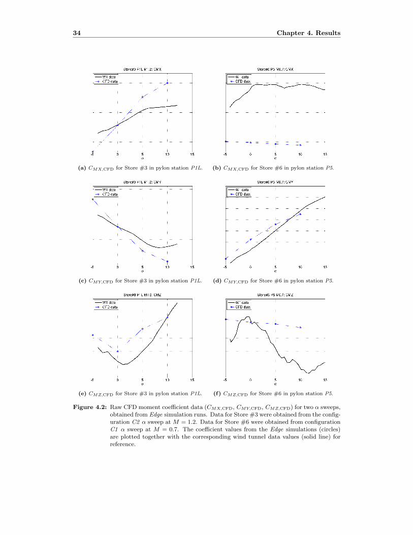
34 Chapter 4. Results
(a) CMX,CFD for Store #3 in pylon station P1L. (b) CMX,CFD for Store #6 in pylon station P5.
(c) CMY,CFD for Store #3 in pylon station P1L. (d) CMY,CFD for Store #6 in pylon station P5.
(e) CMZ,CFD for Store #3 in pylon station P1L. (f) CMZ,CFD for Store #6 in pylon station P5.
Figure 4.2: Raw CFD moment coefficient data (CMX,CFD, CMY,CFD, CMZ,CFD) for two α sweeps,obtained from Edge simulation runs. Data for Store #3 were obtained from the config-uration C2 α sweep at M = 1.2. Data for Store #6 were obtained from configurationC1 α sweep at M = 0.7. The coefficient values from the Edge simulations (circles)are plotted together with the corresponding wind tunnel data values (solid line) forreference.
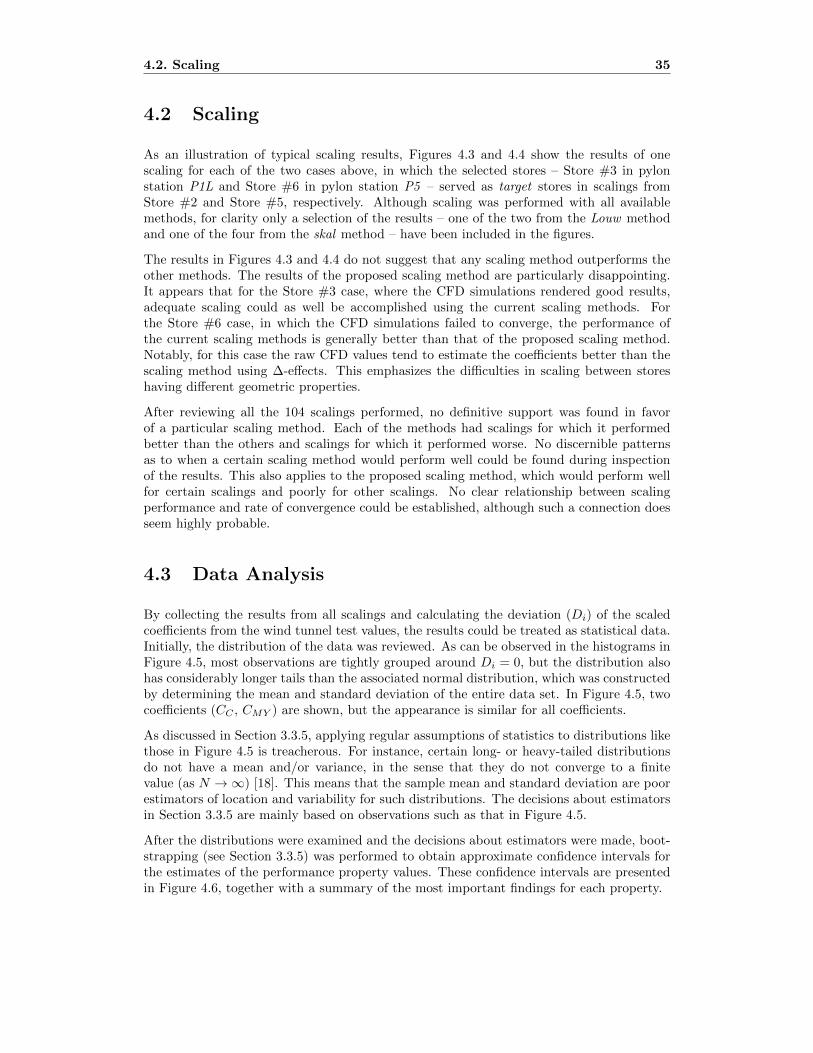
4.2. Scaling 35
4.2 Scaling
As an illustration of typical scaling results, Figures 4.3 and 4.4 show the results of onescaling for each of the two cases above, in which the selected stores – Store #3 in pylonstation P1L and Store #6 in pylon station P5 – served as target stores in scalings fromStore #2 and Store #5, respectively. Although scaling was performed with all availablemethods, for clarity only a selection of the results – one of the two from the Louw methodand one of the four from the skal method – have been included in the figures.
The results in Figures 4.3 and 4.4 do not suggest that any scaling method outperforms theother methods. The results of the proposed scaling method are particularly disappointing.It appears that for the Store #3 case, where the CFD simulations rendered good results,adequate scaling could as well be accomplished using the current scaling methods. Forthe Store #6 case, in which the CFD simulations failed to converge, the performance ofthe current scaling methods is generally better than that of the proposed scaling method.Notably, for this case the raw CFD values tend to estimate the coefficients better than thescaling method using ∆-effects. This emphasizes the difficulties in scaling between storeshaving different geometric properties.
After reviewing all the 104 scalings performed, no definitive support was found in favorof a particular scaling method. Each of the methods had scalings for which it performedbetter than the others and scalings for which it performed worse. No discernible patternsas to when a certain scaling method would perform well could be found during inspectionof the results. This also applies to the proposed scaling method, which would perform wellfor certain scalings and poorly for other scalings. No clear relationship between scalingperformance and rate of convergence could be established, although such a connection doesseem highly probable.
4.3 Data Analysis
By collecting the results from all scalings and calculating the deviation (Di) of the scaledcoefficients from the wind tunnel test values, the results could be treated as statistical data.Initially, the distribution of the data was reviewed. As can be observed in the histograms inFigure 4.5, most observations are tightly grouped around Di = 0, but the distribution alsohas considerably longer tails than the associated normal distribution, which was constructedby determining the mean and standard deviation of the entire data set. In Figure 4.5, twocoefficients (CC , CMY ) are shown, but the appearance is similar for all coefficients.
As discussed in Section 3.3.5, applying regular assumptions of statistics to distributions likethose in Figure 4.5 is treacherous. For instance, certain long- or heavy-tailed distributionsdo not have a mean and/or variance, in the sense that they do not converge to a finitevalue (as N → ∞) [18]. This means that the sample mean and standard deviation are poorestimators of location and variability for such distributions. The decisions about estimatorsin Section 3.3.5 are mainly based on observations such as that in Figure 4.5.
After the distributions were examined and the decisions about estimators were made, boot-strapping (see Section 3.3.5) was performed to obtain approximate confidence intervals forthe estimates of the performance property values. These confidence intervals are presentedin Figure 4.6, together with a summary of the most important findings for each property.
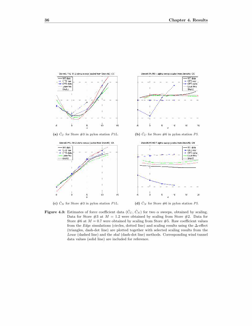
36 Chapter 4. Results
(a) CC for Store #3 in pylon station P1L. (b) CC for Store #6 in pylon station P5.
(c) CN for Store #3 in pylon station P1L. (d) CN for Store #6 in pylon station P5.
Figure 4.3: Estimates of force coefficient data (CC , CN ) for two α sweeps, obtained by scaling.Data for Store #3 at M = 1.2 were obtained by scaling from Store #2. Data forStore #6 at M = 0.7 were obtained by scaling from Store #5. Raw coefficient valuesfrom the Edge simulations (circles, dotted line) and scaling results using the ∆-effect(triangles, dash-dot line) are plotted together with selected scaling results from theLouw (dashed line) and the skal (dash-dot line) methods. Corresponding wind tunneldata values (solid line) are included for reference.
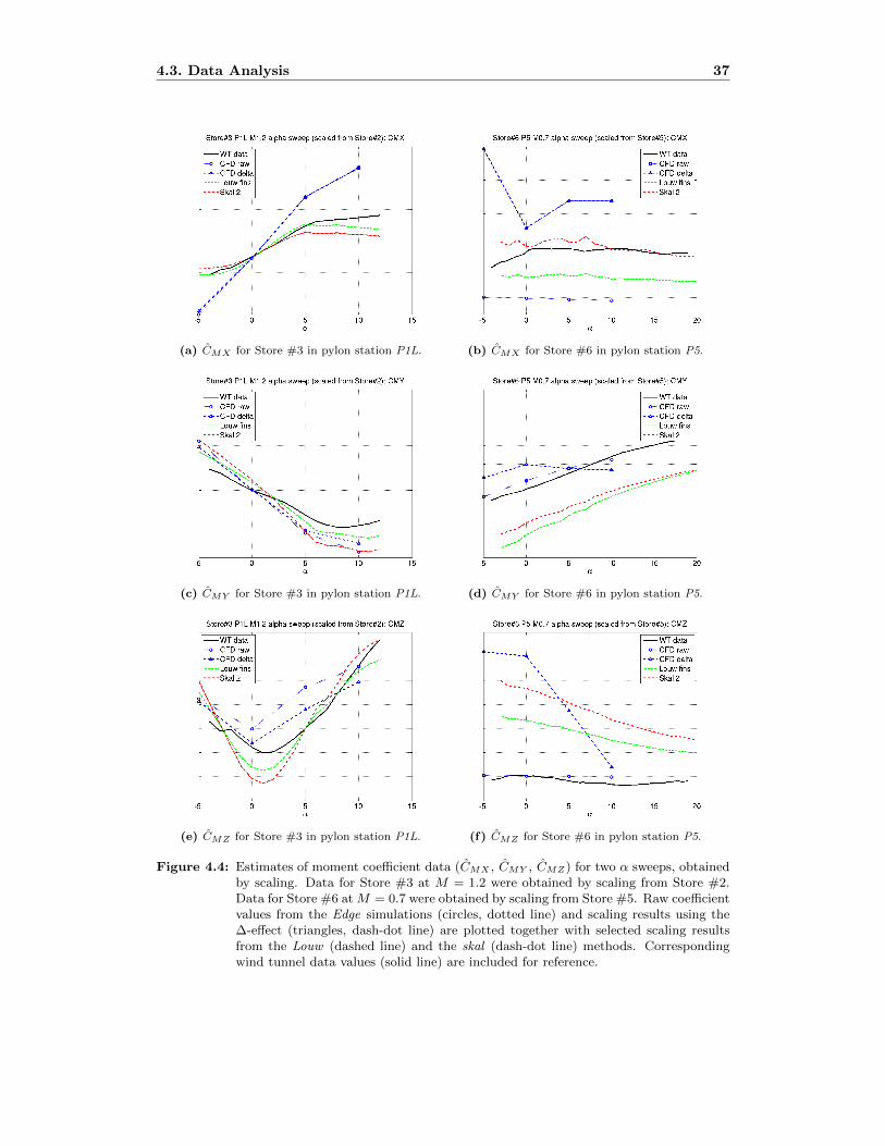
4.3. Data Analysis 37
(a) CMX for Store #3 in pylon station P1L. (b) CMX for Store #6 in pylon station P5.
(c) CMY for Store #3 in pylon station P1L. (d) CMY for Store #6 in pylon station P5.
(e) CMZ for Store #3 in pylon station P1L. (f) CMZ for Store #6 in pylon station P5.
Figure 4.4: Estimates of moment coefficient data (CMX , CMY , CMZ) for two α sweeps, obtainedby scaling. Data for Store #3 at M = 1.2 were obtained by scaling from Store #2.Data for Store #6 atM = 0.7 were obtained by scaling from Store #5. Raw coefficientvalues from the Edge simulations (circles, dotted line) and scaling results using the∆-effect (triangles, dash-dot line) are plotted together with selected scaling resultsfrom the Louw (dashed line) and the skal (dash-dot line) methods. Correspondingwind tunnel data values (solid line) are included for reference.
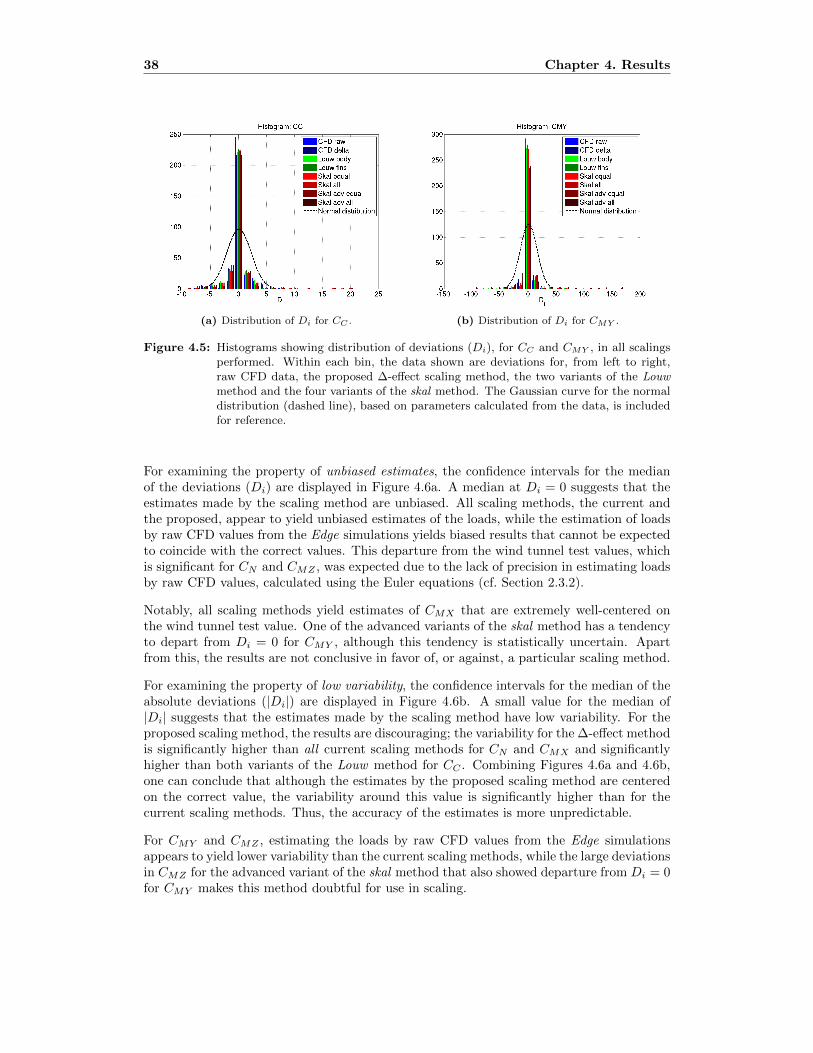
38 Chapter 4. Results
(a) Distribution of Di for CC . (b) Distribution of Di for CMY .
Figure 4.5: Histograms showing distribution of deviations (Di), for CC and CMY , in all scalingsperformed. Within each bin, the data shown are deviations for, from left to right,raw CFD data, the proposed ∆-effect scaling method, the two variants of the Louwmethod and the four variants of the skal method. The Gaussian curve for the normaldistribution (dashed line), based on parameters calculated from the data, is includedfor reference.
For examining the property of unbiased estimates, the confidence intervals for the medianof the deviations (Di) are displayed in Figure 4.6a. A median at Di = 0 suggests that theestimates made by the scaling method are unbiased. All scaling methods, the current andthe proposed, appear to yield unbiased estimates of the loads, while the estimation of loadsby raw CFD values from the Edge simulations yields biased results that cannot be expectedto coincide with the correct values. This departure from the wind tunnel test values, whichis significant for CN and CMZ , was expected due to the lack of precision in estimating loadsby raw CFD values, calculated using the Euler equations (cf. Section 2.3.2).
Notably, all scaling methods yield estimates of CMX that are extremely well-centered onthe wind tunnel test value. One of the advanced variants of the skal method has a tendencyto depart from Di = 0 for CMY , although this tendency is statistically uncertain. Apartfrom this, the results are not conclusive in favor of, or against, a particular scaling method.
For examining the property of low variability, the confidence intervals for the median of theabsolute deviations (|Di|) are displayed in Figure 4.6b. A small value for the median of|Di| suggests that the estimates made by the scaling method have low variability. For theproposed scaling method, the results are discouraging; the variability for the∆-effect methodis significantly higher than all current scaling methods for CN and CMX and significantlyhigher than both variants of the Louw method for CC . Combining Figures 4.6a and 4.6b,one can conclude that although the estimates by the proposed scaling method are centeredon the correct value, the variability around this value is significantly higher than for thecurrent scaling methods. Thus, the accuracy of the estimates is more unpredictable.
For CMY and CMZ , estimating the loads by raw CFD values from the Edge simulationsappears to yield lower variability than the current scaling methods, while the large deviationsin CMZ for the advanced variant of the skal method that also showed departure from Di = 0for CMY makes this method doubtful for use in scaling.
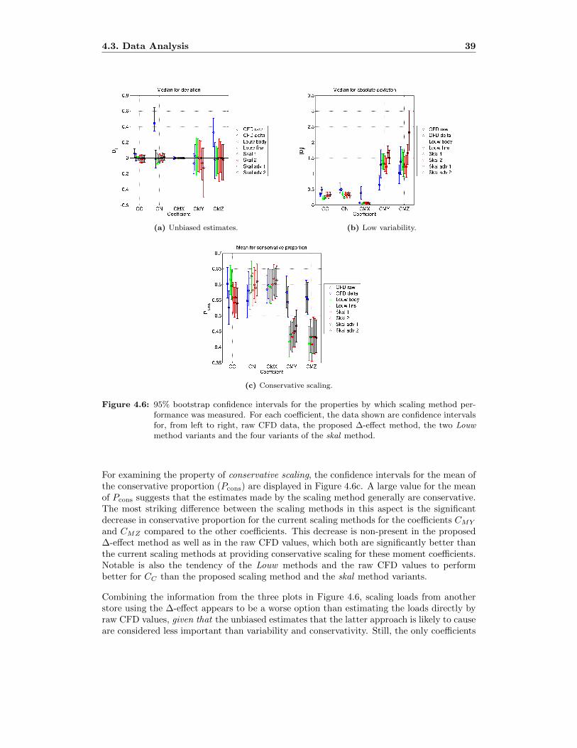
4.3. Data Analysis 39
(a) Unbiased estimates. (b) Low variability.
(c) Conservative scaling.
Figure 4.6: 95% bootstrap confidence intervals for the properties by which scaling method per-formance was measured. For each coefficient, the data shown are confidence intervalsfor, from left to right, raw CFD data, the proposed ∆-effect method, the two Louwmethod variants and the four variants of the skal method.
For examining the property of conservative scaling, the confidence intervals for the mean ofthe conservative proportion (Pcons) are displayed in Figure 4.6c. A large value for the meanof Pcons suggests that the estimates made by the scaling method generally are conservative.The most striking difference between the scaling methods in this aspect is the significantdecrease in conservative proportion for the current scaling methods for the coefficients CMY
and CMZ compared to the other coefficients. This decrease is non-present in the proposed∆-effect method as well as in the raw CFD values, which both are significantly better thanthe current scaling methods at providing conservative scaling for these moment coefficients.Notable is also the tendency of the Louw methods and the raw CFD values to performbetter for CC than the proposed scaling method and the skal method variants.
Combining the information from the three plots in Figure 4.6, scaling loads from anotherstore using the ∆-effect appears to be a worse option than estimating the loads directly byraw CFD values, given that the unbiased estimates that the latter approach is likely to causeare considered less important than variability and conservativity. Still, the only coefficients
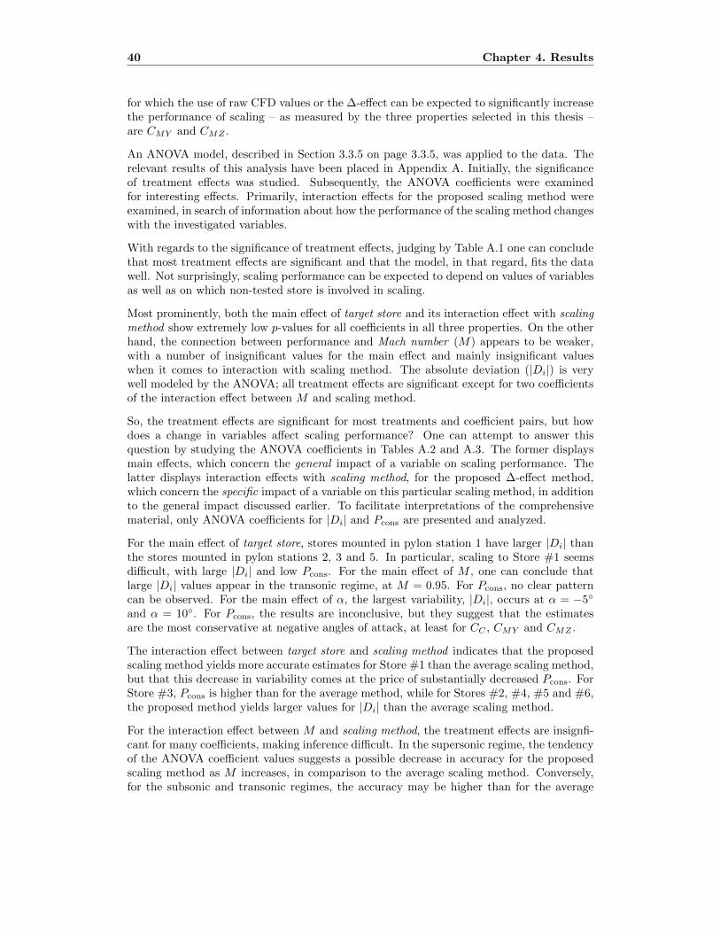
40 Chapter 4. Results
for which the use of raw CFD values or the ∆-effect can be expected to significantly increasethe performance of scaling – as measured by the three properties selected in this thesis –are CMY and CMZ .
An ANOVA model, described in Section 3.3.5 on page 3.3.5, was applied to the data. Therelevant results of this analysis have been placed in Appendix A. Initially, the significanceof treatment effects was studied. Subsequently, the ANOVA coefficients were examinedfor interesting effects. Primarily, interaction effects for the proposed scaling method wereexamined, in search of information about how the performance of the scaling method changeswith the investigated variables.
With regards to the significance of treatment effects, judging by Table A.1 one can concludethat most treatment effects are significant and that the model, in that regard, fits the datawell. Not surprisingly, scaling performance can be expected to depend on values of variablesas well as on which non-tested store is involved in scaling.
Most prominently, both the main effect of target store and its interaction effect with scalingmethod show extremely low p-values for all coefficients in all three properties. On the otherhand, the connection between performance and Mach number (M) appears to be weaker,with a number of insignificant values for the main effect and mainly insignificant valueswhen it comes to interaction with scaling method. The absolute deviation (|Di|) is verywell modeled by the ANOVA; all treatment effects are significant except for two coefficientsof the interaction effect between M and scaling method.
So, the treatment effects are significant for most treatments and coefficient pairs, but howdoes a change in variables affect scaling performance? One can attempt to answer thisquestion by studying the ANOVA coefficients in Tables A.2 and A.3. The former displaysmain effects, which concern the general impact of a variable on scaling performance. Thelatter displays interaction effects with scaling method, for the proposed ∆-effect method,which concern the specific impact of a variable on this particular scaling method, in additionto the general impact discussed earlier. To facilitate interpretations of the comprehensivematerial, only ANOVA coefficients for |Di| and Pcons are presented and analyzed.
For the main effect of target store, stores mounted in pylon station 1 have larger |Di| thanthe stores mounted in pylon stations 2, 3 and 5. In particular, scaling to Store #1 seemsdifficult, with large |Di| and low Pcons. For the main effect of M , one can conclude thatlarge |Di| values appear in the transonic regime, at M = 0.95. For Pcons, no clear patterncan be observed. For the main effect of α, the largest variability, |Di|, occurs at α = −5◦
and α = 10◦. For Pcons, the results are inconclusive, but they suggest that the estimatesare the most conservative at negative angles of attack, at least for CC , CMY and CMZ .
The interaction effect between target store and scaling method indicates that the proposedscaling method yields more accurate estimates for Store #1 than the average scaling method,but that this decrease in variability comes at the price of substantially decreased Pcons. ForStore #3, Pcons is higher than for the average method, while for Stores #2, #4, #5 and #6,the proposed method yields larger values for |Di| than the average scaling method.
For the interaction effect between M and scaling method, the treatment effects are insignfi-cant for many coefficients, making inference difficult. In the supersonic regime, the tendencyof the ANOVA coefficient values suggests a possible decrease in accuracy for the proposedscaling method as M increases, in comparison to the average scaling method. Conversely,for the subsonic and transonic regimes, the accuracy may be higher than for the average
4.3. Data Analysis 41
scaling method. However, there is no statistical support for drawing such conclusions basedon the data presented.
The interaction effect between α and scaling method indicates that the proposed scalingmethod may be more accurate at moderate (positive and negative) angles of attack (α = −5◦
and α = 10◦), and less accurate at the smaller angles, compared to the average scalingmethod. Furthermore, the proposed scaling method yields more conservative estimates atnegative angles of attack than the average method.
After briefly examining the corresponding data for the current scaling methods (consistingof ANOVA data not included in Appendix A), the general impression from the data isthat conservative scaling and low absolute deviations seldom appear simultaneously for anyscaling method/variable pair. In general, it seems that increased accuracy, at least for thescaling methods investigated, comes at the expense of decreased reliability. In addition, thisexamination of the results from the ANOVA study did not yield any conclusive evidencethat promotes a particular scaling method over the other methods.

42 Chapter 4. Results

43
Chapter 5
Conclusions
The main objective of this thesis was to present a scaling method for aerodynamic loadson external stores and/or store configurations, based on the methodology outlined byC. Spjutare (cf. Sections 2.1 and 2.2). As has been displayed in Chapters 3 and 4, sucha method has been presented, implemented and successfully used to estimate loads on anumber of store configurations, with stores mounted in several pylon stations.
However, in order to adopt the proposed scaling method as the new scaling methodologyfor use at the Loads Department, the mere ability to produce results is not enough. Inassessing the usefulness of the scaling method, both the quality of the scalings produced –as measured in thesis by the three performance properties –, the limitations of the scalingmethod and the time required for scaling are relevant factors. These are discussed below.
Due to the absence of evidence supporting the proposed scaling method as the new scalingmethodology, no attempts were made in this thesis to integrate the scaling method with thecurrent tools used for determining loads at the Loads Department. Should the proposedscaling method be implemented, the methods and scripts used for collecting coefficient datafrom the simulations and preparing them for analysis (see Section 3.2.4) may provide ameans for migrating scaled loads data to a database for use in the loads determinationsoftware.
5.1 Scaling Method Performance and Limitations
From the analysis of scaling method performance, no conclusions about definitive improve-ment in scaling performance over the current scaling methods can be drawn, except for asignificant increase in the proportion of conservative scalings when estimating the pitching(CMY ) and yawing (CMZ) moments with the proposed scaling method rather than with thecurrent scaling methods.
The higher degree of conservativity observed for CMY and CMZ in the proposed scalingmethod might be attributed to an ability of the CFD-based scaling method to better capturelocal changes in airflow due to e.g. interference from adjacent surfaces. This could yieldestimates that are qualitatively, albeit not necessarily quantitatively, more correct than the
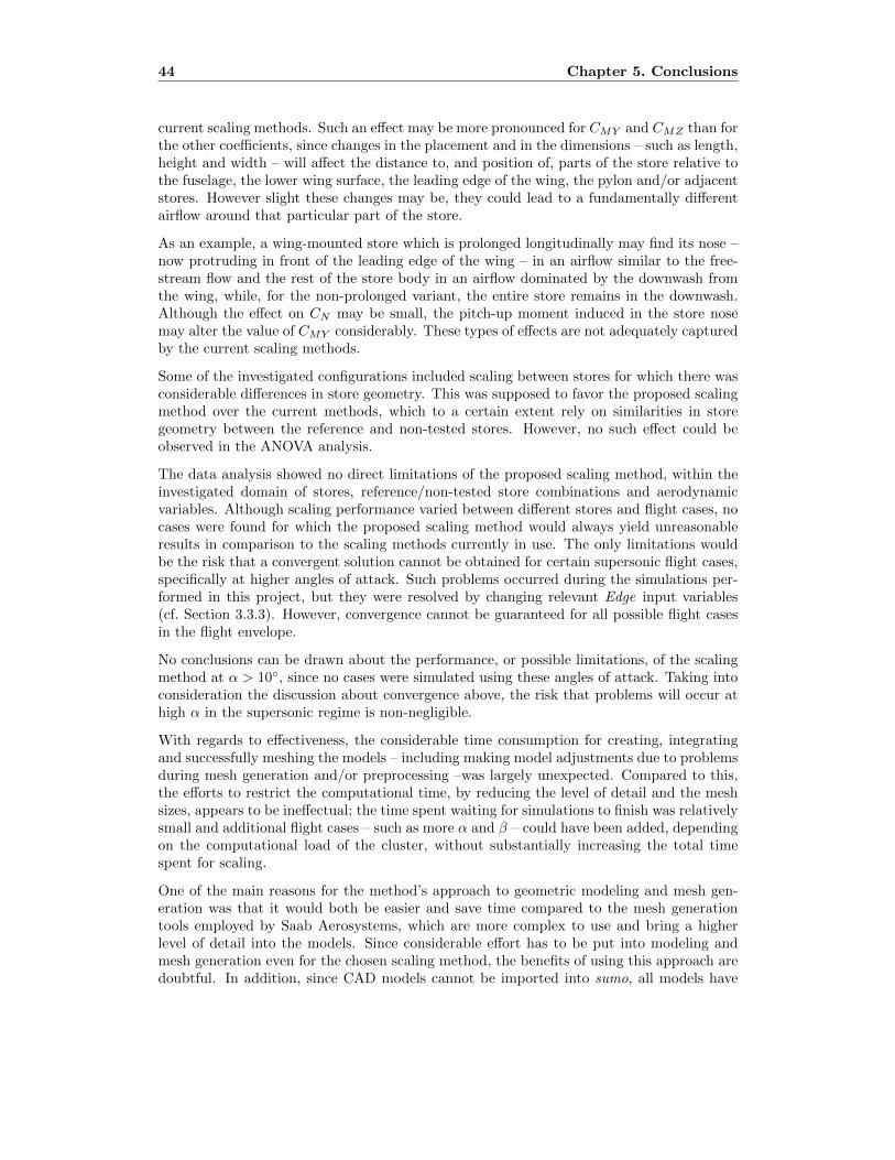
44 Chapter 5. Conclusions
current scaling methods. Such an effect may be more pronounced for CMY and CMZ than forthe other coefficients, since changes in the placement and in the dimensions – such as length,height and width – will affect the distance to, and position of, parts of the store relative tothe fuselage, the lower wing surface, the leading edge of the wing, the pylon and/or adjacentstores. However slight these changes may be, they could lead to a fundamentally differentairflow around that particular part of the store.
As an example, a wing-mounted store which is prolonged longitudinally may find its nose –now protruding in front of the leading edge of the wing – in an airflow similar to the free-stream flow and the rest of the store body in an airflow dominated by the downwash fromthe wing, while, for the non-prolonged variant, the entire store remains in the downwash.Although the effect on CN may be small, the pitch-up moment induced in the store nosemay alter the value of CMY considerably. These types of effects are not adequately capturedby the current scaling methods.
Some of the investigated configurations included scaling between stores for which there wasconsiderable differences in store geometry. This was supposed to favor the proposed scalingmethod over the current methods, which to a certain extent rely on similarities in storegeometry between the reference and non-tested stores. However, no such effect could beobserved in the ANOVA analysis.
The data analysis showed no direct limitations of the proposed scaling method, within theinvestigated domain of stores, reference/non-tested store combinations and aerodynamicvariables. Although scaling performance varied between different stores and flight cases, nocases were found for which the proposed scaling method would always yield unreasonableresults in comparison to the scaling methods currently in use. The only limitations wouldbe the risk that a convergent solution cannot be obtained for certain supersonic flight cases,specifically at higher angles of attack. Such problems occurred during the simulations per-formed in this project, but they were resolved by changing relevant Edge input variables(cf. Section 3.3.3). However, convergence cannot be guaranteed for all possible flight casesin the flight envelope.
No conclusions can be drawn about the performance, or possible limitations, of the scalingmethod at α > 10◦, since no cases were simulated using these angles of attack. Taking intoconsideration the discussion about convergence above, the risk that problems will occur athigh α in the supersonic regime is non-negligible.
With regards to effectiveness, the considerable time consumption for creating, integratingand successfully meshing the models – including making model adjustments due to problemsduring mesh generation and/or preprocessing –was largely unexpected. Compared to this,the efforts to restrict the computational time, by reducing the level of detail and the meshsizes, appears to be ineffectual; the time spent waiting for simulations to finish was relativelysmall and additional flight cases – such as more α and β – could have been added, dependingon the computational load of the cluster, without substantially increasing the total timespent for scaling.
One of the main reasons for the method’s approach to geometric modeling and mesh gen-eration was that it would both be easier and save time compared to the mesh generationtools employed by Saab Aerosystems, which are more complex to use and bring a higherlevel of detail into the models. Since considerable effort has to be put into modeling andmesh generation even for the chosen scaling method, the benefits of using this approach aredoubtful. In addition, since CAD models cannot be imported into sumo, all models have
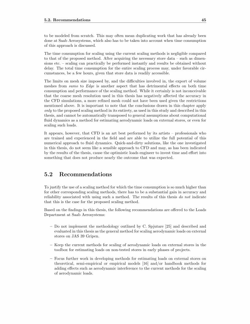
5.2. Recommendations 45
to be modeled from scratch. This may often mean duplicating work that has already beendone at Saab Aerosystems, which also has to be taken into account when time consumptionof this approach is discussed.
The time consumption for scaling using the current scaling methods is negligible comparedto that of the proposed method. After acquiring the necessary store data – such as dimen-sions etc. – scaling can practically be performed instantly and results be obtained withoutdelay. The total time consumption for the entire scaling process may, under favorable cir-cumstances, be a few hours, given that store data is readily accessible.
The limits on mesh size imposed by, and the difficulties involved in, the export of volumemeshes from sumo to Edge is another aspect that has detrimental effects on both timeconsumption and performance of the scaling method. While it certainly is not inconceivablethat the coarse mesh resolution used in this thesis has negatively affected the accuracy inthe CFD simulations, a more refined mesh could not have been used given the restrictionsmentioned above. It is important to note that the conclusions drawn in this chapter applyonly to the proposed scaling method in its entirety, as used in this study and described in thisthesis, and cannot be automatically transposed to general assumptions about computationalfluid dynamics as a method for estimating aerodynamic loads on external stores, or even forscaling such loads.
It appears, however, that CFD is an art best performed by its artists – professionals whoare trained and experienced in the field and are able to utilize the full potential of thisnumerical approach to fluid dynamics. Quick-and-dirty solutions, like the one investigatedin this thesis, do not seem like a sensible approach to CFD and may, as has been indicatedby the results of the thesis, cause the optimistic loads engineer to invest time and effort intosomething that does not produce nearly the outcome that was expected.
5.2 Recommendations
To justify the use of a scaling method for which the time consumption is so much higher thanfor other corresponding scaling methods, there has to be a substantial gain in accuracy andreliability associated with using such a method. The results of this thesis do not indicatethat this is the case for the proposed scaling method.
Based on the findings in this thesis, the following recommendations are offered to the LoadsDepartment at Saab Aerosystems:
– Do not implement the methodology outlined by C. Spjutare [25] and described andevaluated in this thesis as the general method for scaling aerodynamic loads on externalstores on JAS 39 Gripen.
– Keep the current methods for scaling of aerodynamic loads on external stores in thetoolbox for estimating loads on non-tested stores in early phases of projects.
– Focus further work in developing methods for estimating loads on external stores ontheoretical, semi-empirical or empirical models [16] and/or handbook methods foradding effects such as aerodynamic interference to the current methods for the scalingof aerodynamic loads.
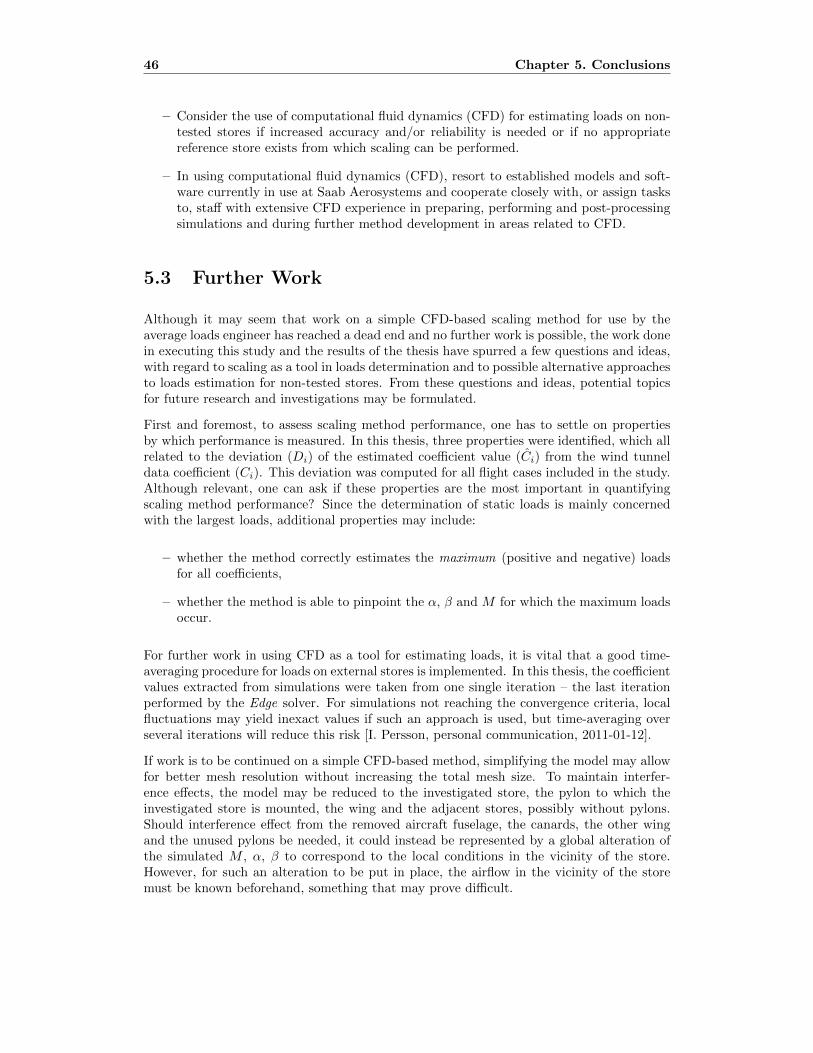
46 Chapter 5. Conclusions
– Consider the use of computational fluid dynamics (CFD) for estimating loads on non-tested stores if increased accuracy and/or reliability is needed or if no appropriatereference store exists from which scaling can be performed.
– In using computational fluid dynamics (CFD), resort to established models and soft-ware currently in use at Saab Aerosystems and cooperate closely with, or assign tasksto, staff with extensive CFD experience in preparing, performing and post-processingsimulations and during further method development in areas related to CFD.
5.3 Further Work
Although it may seem that work on a simple CFD-based scaling method for use by theaverage loads engineer has reached a dead end and no further work is possible, the work donein executing this study and the results of the thesis have spurred a few questions and ideas,with regard to scaling as a tool in loads determination and to possible alternative approachesto loads estimation for non-tested stores. From these questions and ideas, potential topicsfor future research and investigations may be formulated.
First and foremost, to assess scaling method performance, one has to settle on propertiesby which performance is measured. In this thesis, three properties were identified, which allrelated to the deviation (Di) of the estimated coefficient value (Ci) from the wind tunneldata coefficient (Ci). This deviation was computed for all flight cases included in the study.Although relevant, one can ask if these properties are the most important in quantifyingscaling method performance? Since the determination of static loads is mainly concernedwith the largest loads, additional properties may include:
– whether the method correctly estimates the maximum (positive and negative) loadsfor all coefficients,
– whether the method is able to pinpoint the α, β and M for which the maximum loadsoccur.
For further work in using CFD as a tool for estimating loads, it is vital that a good time-averaging procedure for loads on external stores is implemented. In this thesis, the coefficientvalues extracted from simulations were taken from one single iteration – the last iterationperformed by the Edge solver. For simulations not reaching the convergence criteria, localfluctuations may yield inexact values if such an approach is used, but time-averaging overseveral iterations will reduce this risk [I. Persson, personal communication, 2011-01-12].
If work is to be continued on a simple CFD-based method, simplifying the model may allowfor better mesh resolution without increasing the total mesh size. To maintain interfer-ence effects, the model may be reduced to the investigated store, the pylon to which theinvestigated store is mounted, the wing and the adjacent stores, possibly without pylons.Should interference effect from the removed aircraft fuselage, the canards, the other wingand the unused pylons be needed, it could instead be represented by a global alteration ofthe simulated M , α, β to correspond to the local conditions in the vicinity of the store.However, for such an alteration to be put in place, the airflow in the vicinity of the storemust be known beforehand, something that may prove difficult.
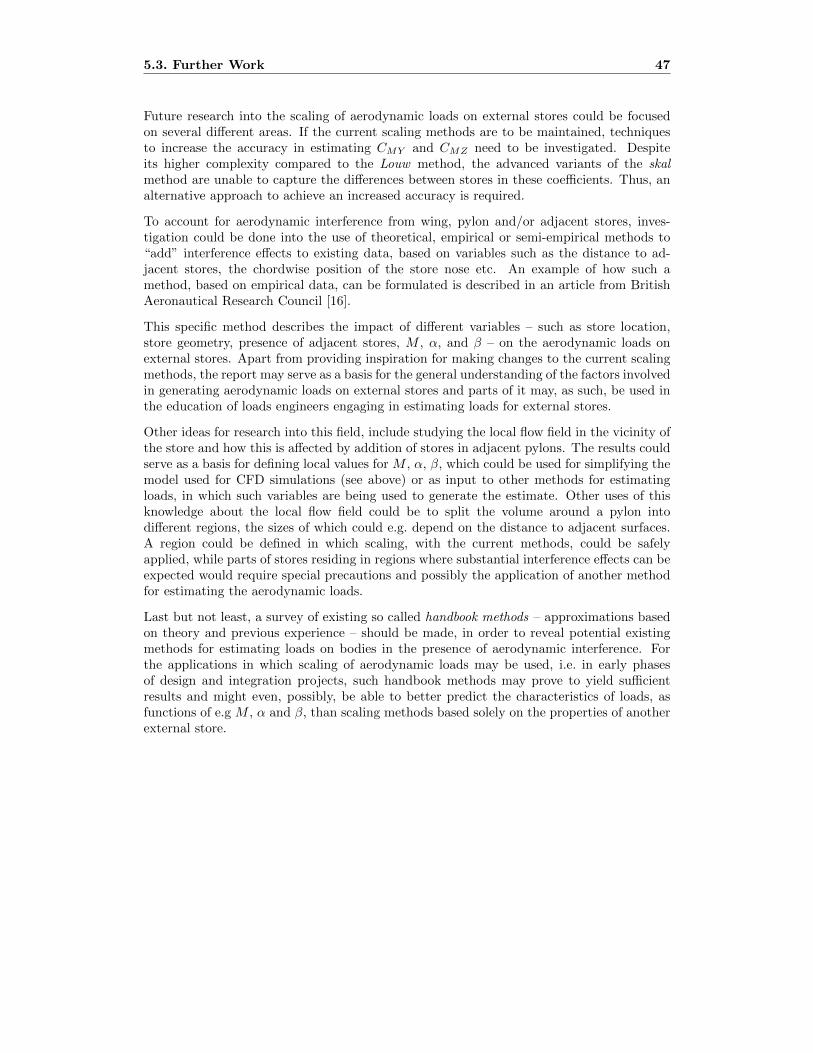
5.3. Further Work 47
Future research into the scaling of aerodynamic loads on external stores could be focusedon several different areas. If the current scaling methods are to be maintained, techniquesto increase the accuracy in estimating CMY and CMZ need to be investigated. Despiteits higher complexity compared to the Louw method, the advanced variants of the skalmethod are unable to capture the differences between stores in these coefficients. Thus, analternative approach to achieve an increased accuracy is required.
To account for aerodynamic interference from wing, pylon and/or adjacent stores, inves-tigation could be done into the use of theoretical, empirical or semi-empirical methods to“add” interference effects to existing data, based on variables such as the distance to ad-jacent stores, the chordwise position of the store nose etc. An example of how such amethod, based on empirical data, can be formulated is described in an article from BritishAeronautical Research Council [16].
This specific method describes the impact of different variables – such as store location,store geometry, presence of adjacent stores, M , α, and β – on the aerodynamic loads onexternal stores. Apart from providing inspiration for making changes to the current scalingmethods, the report may serve as a basis for the general understanding of the factors involvedin generating aerodynamic loads on external stores and parts of it may, as such, be used inthe education of loads engineers engaging in estimating loads for external stores.
Other ideas for research into this field, include studying the local flow field in the vicinity ofthe store and how this is affected by addition of stores in adjacent pylons. The results couldserve as a basis for defining local values for M , α, β, which could be used for simplifying themodel used for CFD simulations (see above) or as input to other methods for estimatingloads, in which such variables are being used to generate the estimate. Other uses of thisknowledge about the local flow field could be to split the volume around a pylon intodifferent regions, the sizes of which could e.g. depend on the distance to adjacent surfaces.A region could be defined in which scaling, with the current methods, could be safelyapplied, while parts of stores residing in regions where substantial interference effects can beexpected would require special precautions and possibly the application of another methodfor estimating the aerodynamic loads.
Last but not least, a survey of existing so called handbook methods – approximations basedon theory and previous experience – should be made, in order to reveal potential existingmethods for estimating loads on bodies in the presence of aerodynamic interference. Forthe applications in which scaling of aerodynamic loads may be used, i.e. in early phasesof design and integration projects, such handbook methods may prove to yield sufficientresults and might even, possibly, be able to better predict the characteristics of loads, asfunctions of e.g M , α and β, than scaling methods based solely on the properties of anotherexternal store.

48 Chapter 5. Conclusions
49
References
[1] J.D. Anderson. Fundamentals of aerodynamics. McGraw-Hill, New York, 1991.
[2] J.D. Anderson. Computational fluid dynamics: The basics with applications. McGraw-Hill, New York, 1995.
[3] M.J. Anderson. A new method for non-parametric multivariate analysis of variance.Austral Ecology, 26(1):32–46, 2001.
[4] W.J. Conover and R.L. Iman. Rank transformations as a bridge between parametricand nonparametric statistics. American Statistician, 35(3):124–129, 1981.
[5] R. Courant, K. Friedrichs, and H. Lewy. On the partial difference equations of mathe-matical physics. IBM Journal of Research and Development, 11(2):215–234, 2010.
[6] B. Efron. Bootstrap methods: Another look at the jackknife. The annals of Statistics,pages 1–26, 1979.
[7] D. Eller. Sumo: Aircraft geometry and surface modeling. http://www.larosterna.com/sumo.html, 2009. retrieved February 11, 2011.
[8] FOI. Edge: Theoretical formulation, version 4.1.0 edition, 2007.
[9] FOI. Edge: User guide, version 4.1.0 edition, 2007.
[10] M. Friedman. The use of ranks to avoid the assumption of normality implicit in theanalysis of variance. Journal of the American Statistical Association, 32(200):675–701,1937.
[11] R. Grimes, E. Walsh, D. Quin, and M. Davies. Effect of geometric scaling on aerody-namic performance. AIAA journal, 43(11):2293–2298, 2005.
[12] M.R. Harwell, E.N. Rubinstein, W.S. Hayes, and C.C. Olds. Summarizing Monte Carloresults in methodological research: The one-and two-factor fixed effects ANOVA cases.Journal of Educational and Behavioral Statistics, 17(4):315, 1992.
[13] T.P. Hettmansperger, J.W. McKean, and S.J. Sheather. Robust nonparametric meth-ods. Journal of the American Statistical Association, 95(452), 2000.
[14] K. Karling. Aerodynamiska grundbegrepp: kompendium och handbok. K. Karling,Linkoping, 12th (extended) edition, 2008.
50 REFERENCES
[15] E.L. Lehmann and J.P. Romano. Testing statistical hypotheses. Springer Verlag, NewYork, 2005.
[16] P. Marsden and A.B. Haines. Aerodynamic loads on external stores: A review ofexperimental data and method of prediction. Aeronautical Research Council Reportsand Memoranda, 1962(3503), 1967.
[17] M.M. Munk. The aerodynamic forces on airship hulls. NASA Reference Publication,page 111, 1979.
[18] J.P. Nolan. Stable Distributions: Models for Heavy Tailed Data. Birkhauser,Boston, 2011. In progress, Chapter 1 available at http://academic2.american.edu/
~jpnolan/stable/.
[19] NSC. NSC: Systems. http://www.nsc.liu.se/systems/, 2010. retrieved February 11,2011.
[20] S.J. Owen. A survey of unstructured mesh generation technology. In Proceedings of the7th International Meshing Roundtable, volume 3, pages 239–267, 1998.
[21] K. Pettersson and A. Rizzi. Aerodynamic scaling to free flight conditions: Past andpresent. Progress in Aerospace Sciences, 44(4):295–313, 2008.
[22] J.R. Shewchuk. Tetrahedral mesh generation by Delaunay refinement. In Proceedingsof the 14th Annual Symposium on Computational Geometry, pages 86–95, 1998.
[23] H. Si. TetGen: A quality tetrahedral mesh generator and 3D Delaunay triangulator,version 1.4 edition, 2006.
[24] H. Si and K. Gartner. Meshing piecewise linear complexes by constrained Delaunaytetrahedralizations. In Proceedings of the 14th International Meshing Roundtable, pages147–163, 2005.
[25] C. Spjutare. Aerodynamic loads on external stores – Saab 39 Gripen: Evaluationof CFD methods for estimating loads on external stores. Master’s thesis, LinkopingUniversity, 2009.
[26] G.L. Thompson. A note on the rank transform for interactions. Biometrika, 78(3):697,1991.
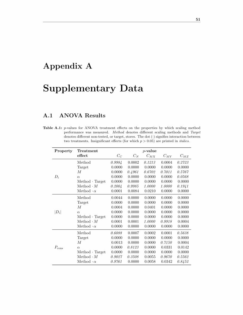
51
Appendix A
Supplementary Data
A.1 ANOVA Results
Table A.1: p-values for ANOVA treatment effects on the properties by which scaling methodperformance was measured. Method denotes different scaling methods and Targetdenotes different non-tested, or target, stores. The dot (·) signifies interaction betweentwo treatments. Insignificant effects (for which p > 0.05) are printed in italics.
Property Treatment p-value
effect CC CN CMX CMY CMZ
Di
Method 0.9984 0.0002 0.1213 0.0004 0.2723Target 0.0000 0.0000 0.0000 0.0000 0.0000M 0.0000 0.4961 0.6702 0.7011 0.5767α 0.0000 0.0000 0.0000 0.0000 0.0568Method · Target 0.0000 0.0000 0.0000 0.0000 0.0000Method ·M 0.2004 0.9985 1.0000 1.0000 0.1941Method ·α 0.0001 0.0084 0.0210 0.0000 0.0000
|Di|
Method 0.0044 0.0000 0.0000 0.0000 0.0000Target 0.0000 0.0000 0.0000 0.0000 0.0000M 0.0004 0.0000 0.0401 0.0000 0.0000α 0.0000 0.0000 0.0000 0.0000 0.0000Method · Target 0.0000 0.0000 0.0000 0.0000 0.0000Method ·M 0.0001 0.0001 1.0000 0.9918 0.0004Method ·α 0.0000 0.0000 0.0000 0.0000 0.0000
Pcons
Method 0.6088 0.0007 0.0002 0.0001 0.5638Target 0.0000 0.0000 0.0000 0.0000 0.0000M 0.0013 0.0000 0.0000 0.7150 0.0004α 0.0000 0.8123 0.0000 0.0331 0.0142Method · Target 0.0000 0.0000 0.0000 0.0000 0.0000Method ·M 0.9027 0.3508 0.0055 0.9670 0.5562Method ·α 0.9761 0.0000 0.0058 0.0342 0.8452
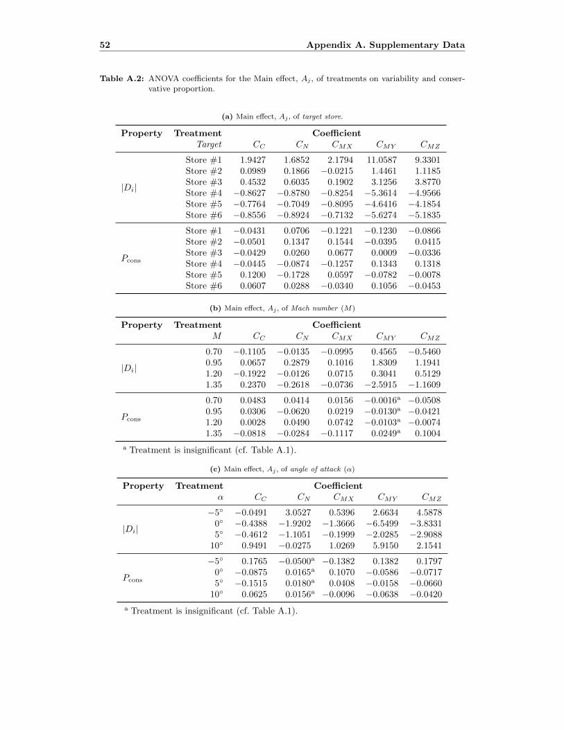
52 Appendix A. Supplementary Data
Table A.2: ANOVA coefficients for the Main effect, Aj , of treatments on variability and conser-vative proportion.
(a) Main effect, Aj , of target store.
Property Treatment Coefficient
Target CC CN CMX CMY CMZ
|Di|
Store #1 1.9427 1.6852 2.1794 11.0587 9.3301Store #2 0.0989 0.1866 −0.0215 1.4461 1.1185Store #3 0.4532 0.6035 0.1902 3.1256 3.8770Store #4 −0.8627 −0.8780 −0.8254 −5.3614 −4.9566Store #5 −0.7764 −0.7049 −0.8095 −4.6416 −4.1854Store #6 −0.8556 −0.8924 −0.7132 −5.6274 −5.1835
Pcons
Store #1 −0.0431 0.0706 −0.1221 −0.1230 −0.0866Store #2 −0.0501 0.1347 0.1544 −0.0395 0.0415Store #3 −0.0429 0.0260 0.0677 0.0009 −0.0336Store #4 −0.0445 −0.0874 −0.1257 0.1343 0.1318Store #5 0.1200 −0.1728 0.0597 −0.0782 −0.0078Store #6 0.0607 0.0288 −0.0340 0.1056 −0.0453
(b) Main effect, Aj , of Mach number (M)
Property Treatment Coefficient
M CC CN CMX CMY CMZ
|Di|
0.70 −0.1105 −0.0135 −0.0995 0.4565 −0.54600.95 0.0657 0.2879 0.1016 1.8309 1.19411.20 −0.1922 −0.0126 0.0715 0.3041 0.51291.35 0.2370 −0.2618 −0.0736 −2.5915 −1.1609
Pcons
0.70 0.0483 0.0414 0.0156 −0.0016a −0.05080.95 0.0306 −0.0620 0.0219 −0.0130a −0.04211.20 0.0028 0.0490 0.0742 −0.0103a −0.00741.35 −0.0818 −0.0284 −0.1117 0.0249a 0.1004
a Treatment is insignificant (cf. Table A.1).
(c) Main effect, Aj , of angle of attack (α)
Property Treatment Coefficient
α CC CN CMX CMY CMZ
|Di|
−5◦ −0.0491 3.0527 0.5396 2.6634 4.58780◦ −0.4388 −1.9202 −1.3666 −6.5499 −3.83315◦ −0.4612 −1.1051 −0.1999 −2.0285 −2.9088
10◦ 0.9491 −0.0275 1.0269 5.9150 2.1541
Pcons
−5◦ 0.1765 −0.0500a −0.1382 0.1382 0.17970◦ −0.0875 0.0165a 0.1070 −0.0586 −0.07175◦ −0.1515 0.0180a 0.0408 −0.0158 −0.0660
10◦ 0.0625 0.0156a −0.0096 −0.0638 −0.0420
a Treatment is insignificant (cf. Table A.1).
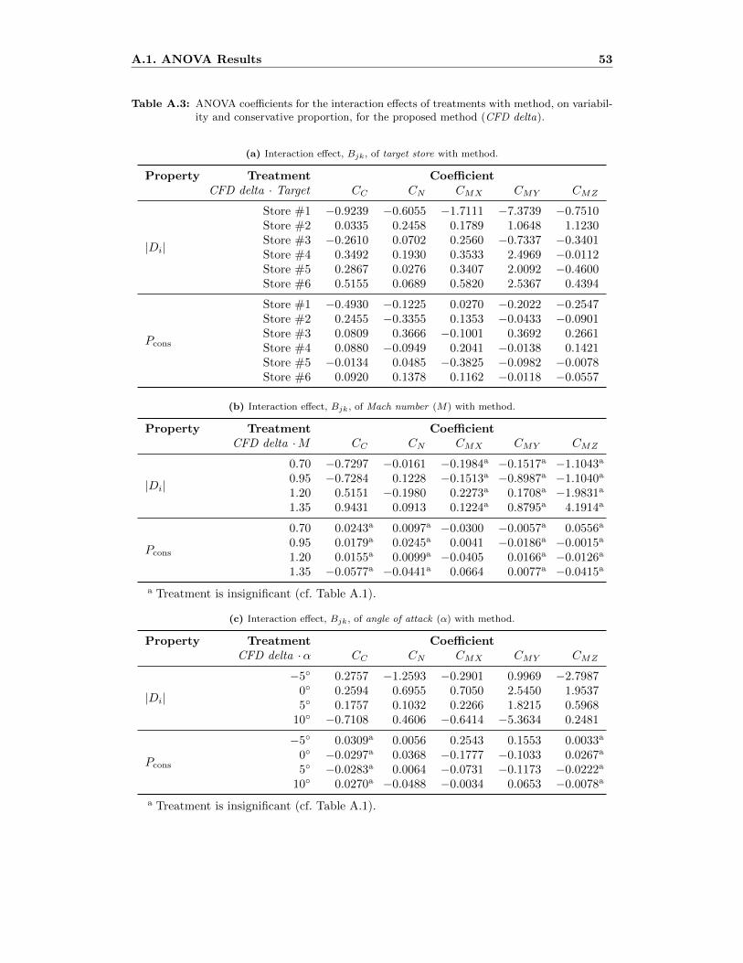
A.1. ANOVA Results 53
Table A.3: ANOVA coefficients for the interaction effects of treatments with method, on variabil-ity and conservative proportion, for the proposed method (CFD delta).
(a) Interaction effect, Bjk, of target store with method.
Property Treatment Coefficient
CFD delta · Target CC CN CMX CMY CMZ
|Di|
Store #1 −0.9239 −0.6055 −1.7111 −7.3739 −0.7510Store #2 0.0335 0.2458 0.1789 1.0648 1.1230Store #3 −0.2610 0.0702 0.2560 −0.7337 −0.3401Store #4 0.3492 0.1930 0.3533 2.4969 −0.0112Store #5 0.2867 0.0276 0.3407 2.0092 −0.4600Store #6 0.5155 0.0689 0.5820 2.5367 0.4394
Pcons
Store #1 −0.4930 −0.1225 0.0270 −0.2022 −0.2547Store #2 0.2455 −0.3355 0.1353 −0.0433 −0.0901Store #3 0.0809 0.3666 −0.1001 0.3692 0.2661Store #4 0.0880 −0.0949 0.2041 −0.0138 0.1421Store #5 −0.0134 0.0485 −0.3825 −0.0982 −0.0078Store #6 0.0920 0.1378 0.1162 −0.0118 −0.0557
(b) Interaction effect, Bjk, of Mach number (M) with method.
Property Treatment Coefficient
CFD delta ·M CC CN CMX CMY CMZ
|Di|
0.70 −0.7297 −0.0161 −0.1984a −0.1517a −1.1043a
0.95 −0.7284 0.1228 −0.1513a −0.8987a −1.1040a
1.20 0.5151 −0.1980 0.2273a 0.1708a −1.9831a
1.35 0.9431 0.0913 0.1224a 0.8795a 4.1914a
Pcons
0.70 0.0243a 0.0097a −0.0300 −0.0057a 0.0556a
0.95 0.0179a 0.0245a 0.0041 −0.0186a −0.0015a
1.20 0.0155a 0.0099a −0.0405 0.0166a −0.0126a
1.35 −0.0577a −0.0441a 0.0664 0.0077a −0.0415a
a Treatment is insignificant (cf. Table A.1).
(c) Interaction effect, Bjk, of angle of attack (α) with method.
Property Treatment Coefficient
CFD delta ·α CC CN CMX CMY CMZ
|Di|
−5◦ 0.2757 −1.2593 −0.2901 0.9969 −2.79870◦ 0.2594 0.6955 0.7050 2.5450 1.95375◦ 0.1757 0.1032 0.2266 1.8215 0.5968
10◦ −0.7108 0.4606 −0.6414 −5.3634 0.2481
Pcons
−5◦ 0.0309a 0.0056 0.2543 0.1553 0.0033a
0◦ −0.0297a 0.0368 −0.1777 −0.1033 0.0267a
5◦ −0.0283a 0.0064 −0.0731 −0.1173 −0.0222a
10◦ 0.0270a −0.0488 −0.0034 0.0653 −0.0078a
a Treatment is insignificant (cf. Table A.1).