sts-107 investigation ascent cfd support investigation ascent cfd support ... the investigation...

34th AIAA Fluid Dynamics Conference 28 June - 1 July, 2004 / Portland, Oregon

STS-107 Investigation Ascent CFD Support

Reynaldo J. Gomez∗ and Darby Vicker∗

NASA Johnson Space Center

Houston, Texas

Stuart E. Rogers†, Michael J. Aftosmis‡, and William M. Chan§

NASA Ames Research Center

Moffett Field, California

Robert Meakin¶

US Army AFDD (AMCOM)


Scott Murman‖

ELORET


This paper provides an overview of the computational fluid dynamics analysis of theascent of the Space Shuttle Launch Vehicle during the investigation of the STS-107 accident.The analysis included both steady-state and unsteady calculations performed with theOverflow and Cart3D flow solvers. The unsteady calculations include moving body, sixdegree-of-freedom simulations of foam debris shed from the region of the left bipod-rampof the vehicle. Many such debris trajectories were computed, some of which impacted thevehicle. The analysis provided an estimate of the speed at which such a piece of debriswould strike the wing leading edge of the Shuttle Orbiter. These results were supplied tothe Columbia Accident Investigation Board, and guided the choice of the impact velocityand foam size selected for the foam-firing test done as part of the investigation. Thistesting subsequently showed that it was possible for a piece of foam debris to cause massivedamage to the Shuttle Orbiter wing Reinforced-Carbon-Carbon panels and T-seals, creatinga breach where hot gases could enter the wing structure during reentry.

I. Introduction

On January 16th 2003, the Space Shuttle Columbia began its last mission, designated STS-107. Duringthe ascent, a piece of foam insulation was shed from the external tank and struck the leading edge of the leftwing of the Orbiter. Although it was not known at the time, this foam-debris strike caused enough damageto the wing that Columbia was lost during reentry on February 1st, 2003.1 Despite the fact that the debrisevent was captured on film, there was significant ambiguity as to the size and speed of the debris. Theneed to determine the possible size, speed, and impact location of the debris led NASA and the ColumbiaAccident Investigation Board (CAIB) to utilize Computational Fluid Dynamics (CFD) techniques to analyze

∗Aerospace Engineer. Member AIAA.†Aerospace Engineer. Associate Fellow AIAA.‡Research Scientist. Senior Member AIAA.§Computer Scientist. Senior Member AIAA.¶Senior Staff Scientist. Senior Member AIAA.‖Senior Research Scientist. Member AIAA.This material is declared a work of the U.S. Government and is not subject to copyright protection in the United States.

1 of 15

American Institute of Aeronautics and Astronautics Paper 2004-2226

the event. In addition to simulations of the debris, the investigation considered the aerodynamic forces actingon the foam bipod ramp, and the detailed flow physics during ascent as it searched for clues to the rootcause of the foam shedding.

This analysis utilized the Overflow,2,3 Overflow-D4,5 and Cart3D6,7 simulation tools. Steady-state Over-flow calculations were performed at several flight conditions of the Columbia ascent. These solutions wereused not only to investigate the aerodynamic forces on the vehicle, but also to provide a flowfield for theballistic integration of possible flight paths of debris pieces. This ballistic integration ignores the effect thatthe traveling debris has on the surrounding flowfield, and it assumes that the only aerodynamic force on thedebris is the drag force acting in the direction of the local relative wind vector. Significantly more accurateand more expensive calculations were also used; these were unsteady, moving-body, CFD simulations of theentire flowfield with proper modeling of the aerodynamic forces and moments acting on the debris. Thedebris was allowed six degrees of freedom (6-DOF) of movement in response to these forces and moments.The 6-DOF simulations are capable of showing the effect of the specific debris shape on its trajectory as wellas the effect of the debris on the vehicle’s flowfield.

This paper provides an overview of the ascent CFD work performed at the Johnson Space Center andat Ames Research Center during the investigation of the STS-107 accident. The following sections includea description of the CFD tools used, including the grid-generation, flow solvers, and computer resources.Following this is a summary of the CFD results that were obtained, both steady-state and unsteady calcu-lations. All of the results of this work was provided to the CAIB during the investigation, and was includedin an appendix of the final CAIB report.8

II. History of Shuttle Overflow CFD

The Overflow2,3 code and the chimera grid approach9 has been in use to solve the flow over the integratedSpace Shuttle Launch Vehicle (SSLV) for over 16 years. Buning et al10 first reported results using thisapproach in 1988, and using grid sizes up to 750,000 points, obtained reasonably good comparison withwind-tunnel pressure coefficient (Cp) data. The geometry in their computations consisted solely of the righthalf of the vehicle, and included simplified versions of the Orbiter, the right Solid-Rocket Booster (SRB), andthe External Tank (ET). Over the next several years, this computational model was refined and continuedto be used to study the SSLV ascent flow field, see Pearce et al.11 Slotnick et al12 used this approach tosimulate the SRB plumes, including variable-gamma effects. By 1994, the procedure was refined to includemore geometric detail, and utilized 113 grids and 16 million grid points; see Slotnick et al,13 Gomez andMa,14 and Martin et al.15

III. Tools

This section briefly describes the CFD tools and computational resources used in the current work.

A. Overflow

The Overflow2,3 code solves the Navier-Stokes equations using a finite-difference formulation in body-fittedcurvilinear meshes. The calculations were run using central differencing of the inviscid and the viscous fluxes,and a diagonalized, approximate-factorization, implicit solver. The Spalart-Allmaras turbulence model wasselected. The code was started from initial conditions using full-multi-grid sequencing on three levels, andwas run to steady-state convergence using three-level multi-grid acceleration. The code was executed onan SGI Origin 3000 shared-memory architecture computer, and utilized a multi-level parallelism16 (MLP)algorithm. The MLP code uses native UNIX directives, and two levels of parallelism. The coarse-grainedparallelism consists of splitting the flow solution into groups of zones, such that each group contains nearlythe same number of grid points. On the fine-grained level, each group is assigned a number of CPUs. TheseCPUs execute the code’s “do” loops in parallel. The performance of the MLP version of Overflow has been

2 of 15


shown to scale linearly with increasing number of CPUs beyond 512 CPUs for large problems. Most of thecurrent Overflow calculations used a total of 128 CPUs and 24 groups.

B. Overflow-D

The Overflow-D4,5 code is based on version 1.6au of the NASA standard Overflow, but has been significantlyenhanced to accommodate moving body applications. The Overflow-D enhancements include the followingcapabilities: on-the-fly generation of off-body grid systems; MPI enabled scalable parallel computing; au-tomatic load balancing; aerodynamic force and moment computations; general 6-DOF model; rigid-bodyrelative motion between an arbitrary number of bodies; domain connectivity; solution error estimation; andgrid adaptation in response to body motion and/or estimates of solution error.

Overflow-D employs the “near-body” and “off-body” domain partitioning method described in Refs. 4and 5; these are used here as the basis of discretization of the SSLV. In the approach, the near-body portionof a domain is defined to include the surface geometry of all bodies being considered and the volume ofspace extending a short distance away from the respective surfaces. The construction of near-body gridsand associated inter-grid connectivity is a classical Chimera-style9 decomposition of the near-body domain.It is assumed that near-body grids provide grid-point distributions of sufficient density to accurately resolvethe flow physics of interest (i.e., boundary-layers, vortices, etc.) without the need for refinement. This isa reasonable constraint since near-body grids are only required to extend a short distance away from bodysurfaces.

The off-body portion of the domain is defined to encompass the near-body domain and extend out to thefar-field boundaries of the problem. The off-body domain is filled with overlapping uniform Cartesian gridsof variable levels of refinement. The off-body grid resolution amplification factor between successive levels is2. The near-body plus off-body partitioning approach facilitates grid adaptation in response to proximity ofbody components and/or to estimates of solution error within the topologically simple off-body grid system.

C. Cart3D

The Cart3D6,7 package solves the Euler equations using a finite-volume formulation on unstructured Carte-sian meshes. Mesh generation with Cart3D is fully automated. The package takes as input the triangulatedsurface geometry and generates an unstructured Cartesian volume mesh by subdividing the computationaldomain based upon the geometry, and any pre-specified regions of mesh refinement. In this manner, thespace near regions of high surface curvature contains highly-refined cells, while areas away from geometry andpre-specified regions contain coarser cells. The intersection of the solid geometry with the regular Cartesianhexahedra is computed, and polyhedral cells are formed which contain the swatch of surface geometry cov-ered by the Cartesian hexahedra. Cells interior to the geometry are automatically removed. The solid-wallboundary conditions for the flow solver are then specified within these “cut-cell” polyhedra. The volumemeshing procedure is robust,6 and does not require user intervention. The meshing scheme is extremely fast(over 1 million cells-per-minute) and meshes are usually created on-demand in the run script and not storedafter the computation has completed. Cart3D’s solver is based on an explicit multi-stage procedure withmultigrid acceleration. Convergence of this solver is comparable with the fastest multigrid solvers in theliterature.7 Cart3D is parallelized using a domain decomposition strategy based upon the use of space-fillingcurves. This approach leads to excellent scalability using either OpenMP7 or MPI17 for communicationon distributed and shared memory computers.18 Prototypes of the moving-body enhancements and 6-DOFmodule used in Cart3D were presented in 2002 and 2003.19−21

D. Computational Resources

Nearly all of the calculations presented in the current work were performed on a 1024-CPU SGI Origin 3000at the NASA Advanced Supercomputer (NAS) facility at Ames Research Center. Due to the urgency ofthese calculations, these jobs were run in a special high-priority batch queue permitting continuous running

3 of 15


and resulting in a very rapid turn-around of the results. This, combined with the gigabit ethernet connectionfrom the Origin to a group of workstations and the excellent support from the NAS staff, resulted in anideal computing environment for this investigation. Additional computing time for the initial Overflow-Dcalculations was provided by the U.S. Army Research Laboratory Major Shared Resource Center.

IV. Geometry and Grid Generation

Figure 1. Photo of the SSLV and the foam bipod ramp.

Figure 1 shows a view of the entire SpaceShuttle Launch Vehicle (SSLV). The com-putational models in the current work in-cluded all of the main components of theSSLV, including the Orbiter, the ET, andthe SRBs. Also included were the majorattach hardware between the components,and most importantly, the left foam bipodramp which was the source of the foam de-bris. The details of the overset and Carte-sian grids are given in the following two sub-sections.

A. Overset Grid Generation

The current investigation work began byupdating the Shuttle ascent overset gridgeneration to include several new featuresand to provide automation of the solutionprocess. These upgrades to the overset-gridgeneration had begun before 2003, but wereaccelerated shortly after the STS-107 acci-dent in order to provide the needed capabil-ity for the current work. The new capabili-ties included a number of improvements tothe geometry and the overset grid topolo-gies. One such improvement was the abil-ity to deflect automatically the four Orbiterelevons and the body flap to any desired op-erational angle and build high-fidelity sur-face grids around the resulting geometry.This was accomplished using a series ofscripts and programs which can reliablyproduce usable grids for any combinationof deflection of these control surfaces, anexample of which is shown in figure 2. An-other improvement was the refinement of the grids around the left-bipod strut and ramp. Previous to theSTS-107 investigation, the grids covering this area were quite coarse and most of the geometric detail wasomitted. As part of the the current work, this area was greatly refined in an effort to compute the aerody-namic forces acting on the bipod ramp. Figure 3 shows a close-up of the resulting grids on the left bipodstrut and ramp. The maximum surface-grid spacing on the bipod ramp is 1.6 inches.

Another major improvement to the grid-generation process was the implementation of the Chimera GridTools (CGT)22,23 scripting system. This provided an easy method of configuration control, the ability

4 of 15


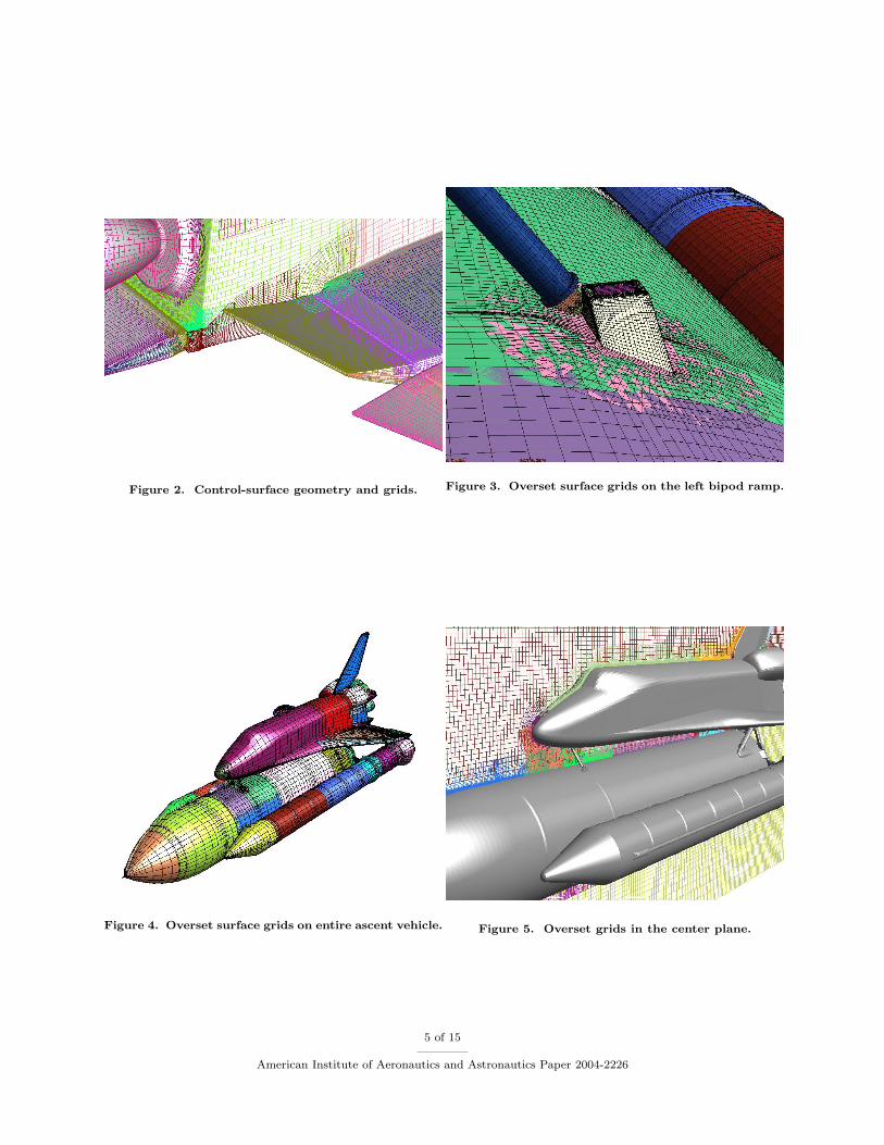
Figure 2. Control-surface geometry and grids. Figure 3. Overset surface grids on the left bipod ramp.

Figure 4. Overset surface grids on entire ascent vehicle. Figure 5. Overset grids in the center plane.

5 of 15


to automate the building of the volume grids, and the ability to automatically generate the necessaryinput files for all of the software programs used in the grid pre-processing, the running of the Overflowsolver, and the final post-processing. The CGT scripts are written using the Tcl scripting language. Thecurrent implementation includes the ability to select specific vehicle configurations with or without certaincomponents such as the SRB, the ET, and various attach hardware. Once the configuration has been selectedand the volume grids are generated, the individual grids are connected using the Pegasus5 software.24

Figure 6. Cartesian mesh with 4.5 million cellsshowing mesh partitioning into 16 subdomains.

A view of the surface grids on the entire ascent vehi-cle configuration is shown in figure 4, which plots everyfourth grid line in each direction for clarity. The typ-ical surface-grid spacing is approximately four inches.The wall-normal spacing of all of the volume grids is1.6 × 10−4 inches. The complete grid system for thisconfiguration is composed of 167 zones and just over 24million grid points. A view of the grids in the centerplane of the vehicle is shown in figure 5.

V. Cartesian Grid Generation

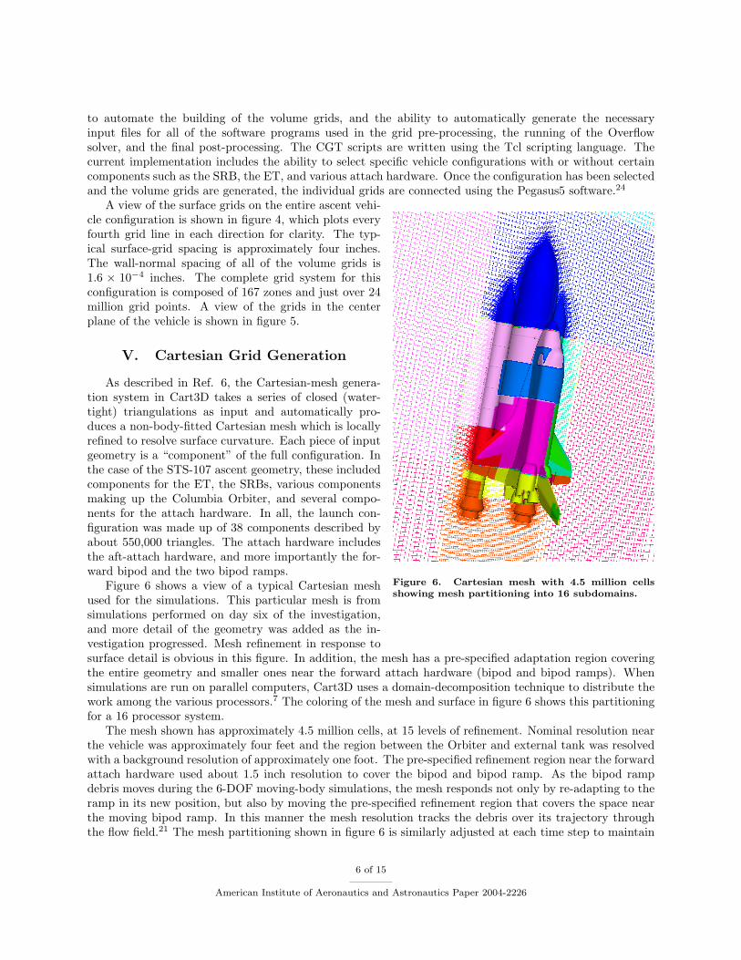
As described in Ref. 6, the Cartesian-mesh genera-tion system in Cart3D takes a series of closed (water-tight) triangulations as input and automatically pro-duces a non-body-fitted Cartesian mesh which is locallyrefined to resolve surface curvature. Each piece of inputgeometry is a “component” of the full configuration. Inthe case of the STS-107 ascent geometry, these includedcomponents for the ET, the SRBs, various componentsmaking up the Columbia Orbiter, and several compo-nents for the attach hardware. In all, the launch con-figuration was made up of 38 components described byabout 550,000 triangles. The attach hardware includesthe aft-attach hardware, and more importantly the for-ward bipod and the two bipod ramps.

Figure 6 shows a view of a typical Cartesian meshused for the simulations. This particular mesh is fromsimulations performed on day six of the investigation,and more detail of the geometry was added as the in-vestigation progressed. Mesh refinement in response tosurface detail is obvious in this figure. In addition, the mesh has a pre-specified adaptation region coveringthe entire geometry and smaller ones near the forward attach hardware (bipod and bipod ramps). Whensimulations are run on parallel computers, Cart3D uses a domain-decomposition technique to distribute thework among the various processors.7 The coloring of the mesh and surface in figure 6 shows this partitioningfor a 16 processor system.

The mesh shown has approximately 4.5 million cells, at 15 levels of refinement. Nominal resolution nearthe vehicle was approximately four feet and the region between the Orbiter and external tank was resolvedwith a background resolution of approximately one foot. The pre-specified refinement region near the forwardattach hardware used about 1.5 inch resolution to cover the bipod and bipod ramp. As the bipod rampdebris moves during the 6-DOF moving-body simulations, the mesh responds not only by re-adapting to theramp in its new position, but also by moving the pre-specified refinement region that covers the space nearthe moving bipod ramp. In this manner the mesh resolution tracks the debris over its trajectory throughthe flow field.21 The mesh partitioning shown in figure 6 is similarly adjusted at each time step to maintain

6 of 15


load balance as the mesh and geometry evolve.

VI. Steady-State Solutions

Figure 7. Cp comparison at Phi = 157.5 deg.

Figure 8. Cp comparison at Phi = 180.0 deg.

Steady-state Overflow and Cart3Dcalculations were performed for anumber of flight conditions expe-rienced along the STS-107 ascenttrajectory. The Mach numbers ofthese conditions ranged from 0.6 to4.0, and included the maximum dy-namic pressure condition at Mach= 1.25, and the conditions at a mis-sion elapsed time (MET) of 81.7seconds. This is the MET whenthe bipod-ramp foam was seen toshed from the ET and fly back andimpact the left wing of the Or-biter. This occurred at an altitudeof 65,820 feet, traveling at Mach =2.46 and a velocity of 2324 feet/sec.Each steady-state Overflow run re-quired about 1000 SGI Origin CPUhours.

A. Validation

In order to validate the currentCFD results, extensive compar-isons of (Cp) between Overflow cal-culations and existing experimen-tal and flight data have been made.These include comparisons of inte-grated forces and moments, and ofCp data covering the Orbiter, ET,and SRB components. A presenta-tion of all of this data is beyondthe scope of this paper. In gen-eral, very good agreement is seenbetween the experimental and com-putational results. Plots of the Cpcomparisons are presented here ontwo axial rows on the ET at circum-ferential angles of 157.5 deg and 180deg, as illustrated in figures 7 and 8. The experimental Cp is plotted with a circle and the CFD resultsare drawn with a solid line. The experimental data comes from the Space Shuttle Program test numberIA-613.25 The comparison is made for a Mach number of 2.50, a Reynolds Number per full-scale inch of6250, an angle of attack of 2.03 deg, and a zero slide-slip angle. These results show that the CFD is in goodagreement with the experimental data.

7 of 15


B. Cart3D and Overflow Comparisons

The following three figures show a comparison of the surface Cp data generated by both Cart3D and Overflowsteady-state solutions. In each of these three figures, the Cart3D Cp is plotted on the left, the Overflow datais plotted on the right, and the difference between the two is shown in the middle. In the color contoursin the middle plots, white represents zero difference between the two; red represents higher pressure in theCart3D solution, and blue represents higher pressure in the Overflow solution. The upper half of each ofthese figures shows the forward third of the ET and SRB surfaces, whereas the lower half shows a closerview of the bipod region of the ET. Figure 9 shows the solutions at a Mach number of 0.6. Mach numbers of1.06 and 2.46 are plotted in figures 10 and 11, respectively. Overall the flow solvers show very similar flowstructure and evidence of shocks in the flow at about the same locations. The effect of the viscosity in theOverflow solutions is seen as the foot-prints of the shocks on the surface Cp are much crisper in the Cart3Dsolutions. Differences due to viscosity increase as the boundary layer gets thicker with increasing altitude. At65,820 feet the Mach=2.46 solutions show the largest local differences: the Overflow solution has a significantamount of flow-separation occurring on the ET surface just upstream of the bipod region. This is due toboth a thicker boundary layer and the intersection of the SRB nose shocks with the Orbiter-nose shock justupstream of the bipod region. This separation results in a dramatically different shock pattern, and largedifferences in the local flow solutions. The viscous Overflow results provide a better representation of theactual flow in this vicinity and so the Overflow computations are used to estimate the actual bipod-rampaerodynamic loads in the following section.

Figure 9. Comparison of Cart3D and Overflow Cp at Mach = 0.6, Alpha = -1.7 deg, Beta = -0.88 deg.

8 of 15


Figure 10. Comparison of Cart3D and Overflow Cp at Mach = 1.06, Alpha = -3.9 deg, Beta = -0.8 deg.

9 of 15


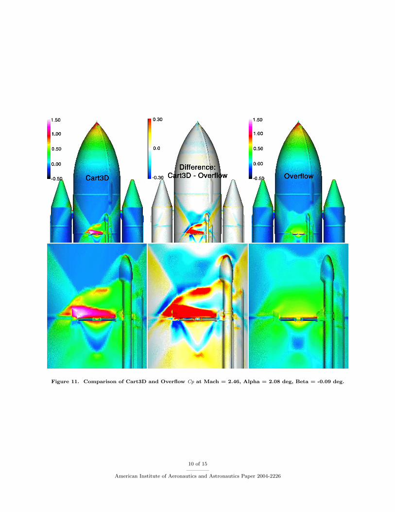
Figure 11. Comparison of Cart3D and Overflow Cp at Mach = 2.46, Alpha = 2.08 deg, Beta = -0.09 deg.

10 of 15


C. Bipod-Ramp loads

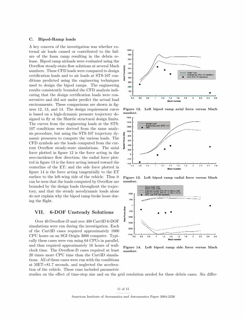
Figure 12. Left bipod ramp axial force versus Machnumber.

Figure 13. Left bipod ramp radial force versus Machnumber.

Figure 14. Left bipod ramp side force versus Machnumber.

A key concern of the investigation was whether ex-ternal air loads caused or contributed to the fail-ure of the foam ramp resulting in the debris re-lease. Bipod ramp airloads were evaluated using theOverflow steady-state flow solutions at several Machnumbers. These CFD loads were compared to designcertification loads and to air loads at STS-107 con-ditions predicted using the engineering techniquesused to design the bipod ramps. The engineeringresults consistently bounded the CFD analysis indi-cating that the design certification loads were con-servative and did not under predict the actual loadenvironments. These comparisons are shown in fig-ures 12, 13, and 14. The design requirement curveis based on a high-dynamic pressure trajectory de-signed to fly at the Shuttle structural design limits.The curves from the engineering loads at the STS-107 conditions were derived from the same analy-sis procedure, but using the STS-107 trajectory dy-namic pressures to compute the various loads. TheCFD symbols are the loads computed from the cur-rent Overflow steady-state simulations. The axialforce plotted in figure 12 is the force acting in thezero-incidence flow direction; the radial force plot-ted in figure 13 is the force acting inward toward thecenterline of the ET; and the side force plotted infigure 14 is the force acting tangentially to the ETsurface to the left-wing side of the vehicle. Thus itcan be seen that the loads computed by Overflow arebounded by the design loads throughout the trajec-tory, and that the steady aerodynamic loads alonedo not explain why the bipod ramp broke loose dur-ing the flight.

VII. 6-DOF Unsteady Solutions

Over 40 Overflow-D and over 400 Cart3D 6-DOFsimulations were run during the investigation. Eachof the Cart3D cases required approximately 1000CPU hours on an SGI Origin 3000 computer. Typi-cally these cases were run using 64 CPUs in parallel,and thus required approximately 16 hours of wall-clock time. The Overflow-D cases required at least20 times more CPU time than the Cart3D simula-tions. All of these cases were run with the conditionsat MET=81.7 seconds, and neglected the accelera-tion of the vehicle. These runs included parametricstudies on the effect of time-step size and on the grid resolution needed for these debris cases. Six differ-

11 of 15


ent specific debris shapes and sizes were simulated, based on the several possible foam-shedding scenarios.These ranged from 167 cubic inches in volume to 1450 cubic inches. Four of these debris pieces are shownin figure 15. For each of these debris shapes, various initial velocity and rotation conditions were applied tothe debris. The debris path was very sensitive to these initial conditions: some combinations of conditionscaused the debris to fly well above and outboard of the wing. Others caused the debris to fly under thewing, or to hit somewhere along the fuselage.

Figure 15. Four of the different debris shapes.

Figure 16. Axial velocities for debris pieces with volumeof 704 cubic inches and different foam densities.

One significant finding of the 6-DOF calcula-tions was that the axial velocity of the debris rel-ative to the vehicle was nearly independent of thedebris initial conditions. Instead, it was primarilydependent on the mass of the debris. This is illus-trated in figure 16 which plots the Cart3D com-puted debris axial velocity versus x-location, mea-sured in the ET-coordinate system, for the 704 cu-bic inch debris shape. The streamwise x-locationof Reinforced-Carbon-Carbon (RCC) panel num-ber eight is about x = 1800 inches, as designatedby the dashed line labeled as the point of impact.This plot shows the effect of changing the debris-material density (and thus its mass). Two trajec-tories are drawn for each density (except the 5.0lbs/ft3 density case), each representing a differentinitial condition. The velocity at x=1800 inchesis relatively independent of the initial condition,but strongly dependent on the density. The re-sults clearly show that the relative axial velocityincreases as the material density decreases.

An example of one Cart3D trajectory whichclosely resembled the strike location seen in theSTS-107 film is shown in figure 17. This is the1450 cubic inch piece of debris. It strikes the left-wing leading edge of the Orbiter on RCC panelnumber eight. The 6-DOF calculations show thatthis debris strikes the wing with a relative veloc-ity of nearly 950 feet/sec. The elapsed time fromthe release of the debris to the impact on the wingis less than 0.15 seconds. During this time, thevelocity of the vehicle increases by less than 10feet/sec, thus neglecting the vehicle accelerationintroduces an error on the order of only one per-cent.

The analysis of the debris as seen on thelaunch video estimates that the foam is travel-ing between 775 and 820 feet/sec. The nominaldensity of the foam used to build the bipod rampsis 2.4 lbs/ft3. As seen in figure 16, the CFD 6-DOF results predict much higher impact veloci-ties than the video analysis for the 704 cubic inchpiece. This result indicates that the debris would have to be significantly larger or of a higher density. Inlarge part due to these CFD results, the CAIB determined that the debris was most likely larger than the

12 of 15


855 cubic inch piece. It was thus decided to use a 1200 cubic inch foam piece during the foam-firing testsinto actual flight RCC panels. These tests ultimately proved that it was possible for a piece of foam to createa massive hole in an RCC panel.1

Figure 17. Cart3D 6-DOF debris trajectory.

The effects of the debris onthe surface pressures of the ve-hicle were estimated by sub-tracting the steady-state so-lution surface pressures fromthose computed during an un-steady trajectory Cart3D com-putation. This analysis showsthat the Orbiter leading-edgepressure is lowered by approx-imately 0.4 psi just before thedebris impact. This is shown infigure 18 which plots color con-tours of the difference in pres-sure on the vehicle surfaces atan instant in time when thedebris is approaching the Or-biter wing leading edge. Redand yellow indicate increasedpressures and cyan and blue in-dicate lowered local pressure.White or gray regions indicatesmall or no change in pressure. The lowered local wing-surface pressure is caused by the wake of the debrispiece that precedes the debris as it travels past a fixed point on the Orbiter wing. Just upstream of this isa higher local pressure region that is caused by the shock formed upstream of the debris piece. This changein local surface pressure may help explain the anomalous accelerations measured on the left-wing outboardelevon accelerometer, which were recorded during the ascent of STS-107 immediately after the debris impactevent.8

VIII. Conclusion

Steady-state computations of the flow field around the Space Shuttle Launch Vehicle during ascent havebeen computed with the Overflow and Cart3D programs. These results have been utilized for simplifiedballistic debris-trajectory computations, and were used to evaluate the air loads on the left bipod ramp.The loads computed by the Overflow code were consistently less than the design requirement loads, andindicate that air loads alone did not cause the bipod ramp to separate from the vehicle. Time-accurate6-DOF moving-body simulations of the bipod-ramp foam debris have been computed with the Cart3D andOverflow-D codes. These simulations helped to define the impact velocity and foam size for the testing doneunder the direction of the CAIB in June of 2003. This testing subsequently showed that is was possible fora piece of foam debris to cause massive damage to the Shuttle Orbiter wing RCC panels and T-seals.

Acknowledgments

This work is dedicated to Astronaut Kalpana Chawla, who perished aboard STS-107. Before she becamean astronaut, Kalpana worked as our colleague at NASA Ames on CFD research in the areas of poweredlift, parallel computing, aerodynamic optimization, and multi-body aerodynamics. She was a good friend

13 of 15


Figure 18. Delta pressure on the vehicle surface caused by debris as computed by Cart3D.

and will be missed.The authors would like to acknowledge the excellent staff and world-class facilities of the NASA Advanced

Supercomputer (NAS) facility at Ames Research Center, which provided us with over 400,000 hours of CPUtime. Thanks also goes to the Department of Defense High-Performance-Computing Modernization Officefor providing 40,000 hours of dedicated CPU time during the first few weeks of the investigation.

References

1 Columbia Accident Investigation Board Report Vol. 1, U.S. Government Printing Office, Washington,DC, Aug. 2003.

2 Kandula, M. and Buning, P. G., “Implementation of LU-SGS Algorithm and Roe Upwinding Schemein OVERFLOW Thin-Layer Navier-Stokes Code,” AIAA Paper 94-2357, AIAA 25th Fluid Dynamics Con-ference, Colorado Springs, CO, June 1994.

3 Jespersen, D. C., Pulliam, T. H., and Buning, P. G., “Recent Enhancements to OVERFLOW,” AIAAPaper 97-0644, Jan. 1997.

4 Meakin, R., “Automatic Off-Body Grid Generation for Domains of Arbitrary Size,” AIAA-2001-2536,15th AIAA Computational Fluid Dynamics Conf., June 2001, Anaheim, CA.

5 Meakin, R., “Adaptive Spatial Partitioning and Refinement for Overset Structured Grids,” Comput.Methods Appl. Mech. Engrg., Vol. 189, pp. 1077-1117, 2000.

6 Aftosmis, M. M., Berger, M. J., and Melton, J. E., “Robust and Efficient Cartesian Mesh Generationfor Component-Based Geometry,” AIAA Journal, Vol. 36, No. 6, pp. 952–960, June 1998, also AIAA Paper97-0196, Jan. 1997.

7 Aftosmis, M.J, Berger M.J., and Adomavicius, G., “A Parallel Multilevel Method for Adaptively RefinedCartesian Grids with Embedded Boundaries,” AIAA Paper 2000-0808, Jan. 2000.

14 of 15


8 Columbia Accident Investigation Board Report Vol. 2, Appendix D.8, pp. 235–271, U.S. GovernmentPrinting Office, Washington, DC, Oct. 2003.

9 Steger, J., Dougherty, C., and Benek, J., “A Chimera Grid Scheme,” Advances in Grid Generation, K.N. Ghia and U. Ghia, eds., ASME FED-Vol 5., June 1983.

10 Buning, P. G., Chiu, I. T., Obayashi, S., Rizk, Y. M., and Steger, J. L., “Numerical Simulation of theIntegrated Space Shuttle Vehicle in Ascent,” AIAA Paper 88-4359-CP, 1988.

11 Pearce, D. G., Stanley, S. A., Martin, F. W., Gomez, R. J., Le Beau, G. J., Buning, P. G., Chan, W.M., Chiu, I. T., Wulf, A. and Akdag, V., “Development of a Large Scale Chimera Grid System for the SpaceShuttle Launch Vehicle,” AIAA Paper 93-0533, 1993.

12 Slotnick, J. P., Kandula, M., Buning, P. G., and Martin, F. W., “Numerical Simulation of the SpaceShuttle Launch Vehicle Flowfield with Real Gas Solid Rocket Motor Plume Effects,” AIAA Paper 93-0521,1993.

13 Slotnick, J. P., Kandula, M. and Buning, P. G., “Navier-Stokes Simulation of the Space ShuttleLaunch Vehicle Flight Transonic Flowfield Using a Large Scale Chimera Grid System,” AIAA Paper 94-1860, Proceedings of the 12th AIAA Applied Aerodynamics Conference, Colorado Springs, Colorado, 1994.

14 Gomez, R. J. and Ma, E. C., “Validation of a Large Scale Chimera Grid System for the Space ShuttleLaunch Vehicle,” AIAA Paper 94-1859, Proceedings of the AIAA 12th Applied Aerodynamics Conference,Colorado Springs, Colorado, 1994.

15 Martin, F. W., Labbe, S. G., Wey, T. C., and Pearce, D. G., “Space Shuttle Launch Vehicle WindTunnel and Flight Aerodynamic Environments,” AIAA Paper 94-1861, Proceedings of the AIAA 12th AppliedAerodynamics Conference, Colorado Springs, Colorado, 1994.

16 Taft, J. R., “Achieving 60 GFLOP/s on the Production CFD Code OVERFLOW-MLP,” ParallelComputing, Vol. 27, No. 4, pp. 521-536, 2001.

17 Marshall, D.D., Aftosmis, M.J., and Ruffin, S.M., “Study of Parallelization Enhancements For ACartesian Grid Solver.” Proceedings of the International conference on Parallel CFD 2002, Kansai ScienceCity, Japan, May 2002.

18 Aftosmis, M.J., Berger, M.J., Murman, S.M., “Applications of Space-Filling Curves to CartesianMethods For CFD,” AIAA Paper 2004-1232, Jan. 2004.

19 Murman, S. M., Aftosmis, M.J., and Berger M.J., “Numerical Simulation of Rolling-Airframes Usinga Multi-Level Cartesian Method,” AIAA Paper 2002-2798, June 2002.

20 Murman, S.M., Aftosmis, M.J., and Berger, M.J., “Implicit Approaches For Moving Boundaries in a3-D Cartesian Method,” AIAA Paper 2003-1119, Jan. 2003.

21 Murman, S.M., Aftosmis, M.J., and Berger, M.J., “Simulations of 6-DOF Motion With a CartesianMethod,” AIAA 2003-1246, Jan. 2003.

22 Rogers, S. E., Roth, K., Nash, S. M., Baker, M. D., Slotnick, J. P., Whitlock, M., and Cao, H. V.,“Advances in Overset CFD Processes Applied to Subsonic High-Lift Aircraft,” AIAA Paper 2000-4216, Aug.2000.

23 Chan, W. M., “The Overgrid Interface for Computational Simulations on Overset Grids,” AIAA Paper2002-3188, June 2002.

24 Rogers, S. E., Suhs, N. E., and Dietz, W. E. “PEGASUS 5: An Automated Pre-processor for Overset-Grid CFD,” AIAA Journal, Vol. 41, No. 6, June 2003, pp. 1037–1045.

25 Marroquin, J. and Lemoine, P., “Results of Wind Tunnel Tests of an ASRM Configured 0.03 ScaleSpace Shuttle Integrated Vehicle Model (47-OTS) in the AEDC 16-foot Transonic Wind Tunnel (IA613A),”NASA Center for Aerospace Information (CASI), NASA-CR-185696, 1992.

15 of 15


sts-107 investigation ascent cfd support investigation ascent cfd support ... the investigation...

Documents