estimation with weak instruments: accuracy of higher order...

Estimation with Weak Instruments: Accuracy of Higher Order

Bias and MSE Approximations1

Jinyong Hahn

Brown University

Jerry Hausman

MIT

Guido Kuersteiner2

MIT

January, 2004

1Please send editorial correspondence to: Guido Kuersteiner, MIT, Department of Economics, E-52-

371A, 50 Memorial Drive, Cambridge, MA 021422Financial support from NSF grant SES-0095132 is gratefully acknowledged.

Abstract

In this paper we consider parameter estimation in a linear simultaneous equations model. It

is well known that two stage least squares (2SLS) estimators may perform poorly when the

instruments are weak. In this case 2SLS tends to suffer from substantial small sample biases.

It is also known that LIML and Nagar-type estimators are less biased than 2SLS but suffer

from large small sample variability. We construct a bias corrected version of 2SLS based on the

Jackknife principle. Using higher order expansions we show that the MSE of our Jackknife 2SLS

estimator is approximately the same as the MSE of the Nagar-type estimator. We also compare

the Jackknife 2SLS with an estimator suggested by Fuller (1977) that signiÞcantly decreases the

small sample variability of LIML. Monte Carlo simulations show that even in relatively large

samples the MSE of LIML and Nagar can be substantially larger than for Jackknife 2SLS. The

Jackknife 2SLS estimator and Fullers estimator give the best overall performance. Based on

our Monte Carlo experiments we conduct formal statistical tests of the accuracy of approximate

bias and MSE formulas. We Þnd that higher order expansions traditionally used to rank LIML,

2SLS and other IV estimators are unreliable when identiÞcation of the model is weak. Overall,

our results show that only estimators with well deÞned Þnite sample moments should be used

when identiÞcation of the model is weak.

Keywords: weak instruments, higher order expansions, bias reduction, Jackknife, 2SLS

JEL C13,C21,C31,C51

1 Introduction

Over the past few years there has been renewed interest in Þnite sample properties of econo-

metric estimators. Most of the related research activities in this area are concentrated in the

investigation of Þnite sample properties of instrumental variables (IV) estimators. It has been

found that standard large sample inference based on 2SLS can be quite misleading in small

samples when the endogenous regressor is only weakly correlated with the instrument. A partial

list of such research activities is Nelson and Startz (1990), Maddala and Jeong (1992), Staiger

and Stock (1997), and Hahn and Hausman (2002).

A general result is that controlling for bias can be quite important in small sample situations.

Anderson and Sawa (1979), Morimune (1983), Bekker (1994), Angrist, Imbens, and Krueger

(1995), and Donald and Newey (2001) found that IV estimators with smaller bias typically have

better risk properties in Þnite sample. For example, it has been found that the LIML, the

JIVE, or Nagars (1959) estimator tend to have much better risk properties than 2SLS. Donald

and Newey (2000), Newey and Smith (2001) and Kuersteiner (2000) may be understood as an

endeavor to obtain a bias reduced version of the GMM estimator in order to improve the Þnite

sample risk properties.

In this paper we consider higher order expansions of LIML, JIVE, Nagar and 2SLS estima-

tors. In addition we contribute to the higher order literature by deriving the higher order risk

properties of the Jackknife 2SLS. Such an exercise is of interest for several reasons. First, we

believe that higher order MSE calculations for the Jackknife estimator have not been available

in the literature. Most papers simply verify the consistency of the Jackknife bias estimator.

See Shao and Tu (1995, Section 2.4) for a typical discussion of this kind. Akahira (1983), who

showed that the Jackknife MLE is second order equivalent to MLE, is closest in spirit to our

exercise here, although a third order expansion is necessary in order to calculate the higher order

MSE.

Second, Jackknife 2SLS may prove to be a reasonable competitor to the LIML or Nagars

estimator despite the fact that higher order theory predicts it should be dominated by LIML.

It is well-known that LIML and Nagars estimator have the moment problem: With normally

distributed error terms, it is known that LIML and Nagar do not possess any moments. See

Mariano and Sawa (1972) or Sawa (1972). On the other hand, it can be shown that Jackknife

2SLS has moments up to the degree of overidentiÞcation. LIML and Nagars estimator have

better higher order risk properties than 2SLS, based on higher order expansions used by Rothen-

berg (1983) or Donald and Newey (2001). These results may however not be very reliable if the

moment problem is not only a feature of the extreme end of the tails but rather affects dispersion

of the estimators more generally. Large dispersions and lack of moments are technically distinct

1

problems, but we identify these problems for historical reasons. On the other hand, these two

problems seem to be identical problems for all practical purpose, as our Monte Carlo results

demonstrate.

We conduct a series of Monte Carlo experiments to determine how well higher order approxi-

mations predict the actual small sample behavior of the different estimators. When identiÞcation

of the model is weak the quality of the approximate MSE formulas based on higher order ex-

pansions turns out to be poor. This is particularly true for the LIML and Nagar estimators

that have no moments in Þnite samples. Our calculations show that estimators that would be

dismissed based on the analysis of higher order stochastic expansions turn out to perform much

better than predicted by theory.

We point out that the literature on exact small sample distributions of 2SLS and LIML such

as Anderson and Sawa (1979), Anderson, Morimune and Sawa (1983), Anderson, Naoto and Sawa

(1982), Holly and Phillips (1979), Phillips (1980) and more recently Oberhelman and Kadiyala

(2000) did not focus on the weak instrument case and therefore the small sample behavior of

LIML under these circumstances is still an open issue. We show that the parametrizations used

in these papers imply values for the Þrst stage R2 that are much larger than typically thought

relevant for the weak instrument case.

These previous papers present Þnite sample results summarized around the concentration

parameter.1 The concentration parameter δ2 is approximately equal to nR2/¡1−R2¢ under

our normalization, where n denotes the sample size.2 In Anderson et. al. (1982, Table I, p.

1012) the minimum concentration parameter equals 30, which far exceeds the weak instrument

cases we consider where the Þrst stage R2 is equal to 0.01. Rather, for the case of n = 100, one

needs R2 = 0.3 in order to get δ2 = 30, which is quite high. Subsequent tables in Anderson et.al.

continue to have this problem with the minimum δ2 = 10 which for R2 = 0.1 means that one

needs n = 1000. Our Monte Carlo experiments show that the weak instrument problem pretty

much disappears for n this large. Similarly, the graphs reported in Anderson et.al., p.1022-1023

do not apply to the weak instrument case because they are based on δ2 = 100 which would

require R2 = 0.1 for n = 1000. The parametrizations of Anderson et. al. were used by other

researchers such as Oberhelman and Kadiyala (2000, p. 171). Anderson and Sawa (1973) use

values of δ2 ranging from 20 to 180 in their numerical work and Anderson and Sawa (1979) use

values of δ2 ranging from 10 to ∞. Holly and Phillips (1979) use δ2 ≥ 40 and Phillips (1980)

considers 2SLS estimators for the case of multiple endogenous variables such that his results

are not directly comparable here. Nevertheless, the implied values of δ2 are roughly 80 with a

sample size of n = 20 which implies an R2 of 0.8.

1The concentration parameter is formally deÞned later on page 11.2See the discussion on page 11.

2

Precisely for the cases with very low Þrst stage R2 we Þnd previously undocumented behavior

of LIML estimators. In particular, LIML tends to be biased and has large inter-quantile ranges

that can dominate those of 2SLS and certainly those of the Jackknife 2SLS advocated here.

Anderson et. al. (1983, p. 233) claim: The inÞnite moments are due to the behavior of

the distributions outside of the range of practical interest to the econometrician. However,

the approximations that they use to reach this conclusion do not work in the weak instrument

case. In particular they claim on p.233 that, The MSE of the asymptotic expansion to order

1/δ2 of the LIML estimator is smaller than that of the TSLS estimator if K2 > 7 and |α| >p2/ (K2 − 7)..., where K2 is the degree of overidentiÞcation. It can be checked easily that

this inequality holds for all the parameter values that we consider in our simulations and we

would thus expect to Þnd smaller interquartile ranges for LIML compared to 2SLS. But quite

to the contrary, our simulation results indicate that LIML does worse than 2SLS in the weak

instrument cases. This is further evidence that the Þnite sample analysis did not address the

weak instrument case. The reason is of course that in the weak instrument case of Staiger and

Stock (1997) δ2 = O(1) such that the approximations analyzed in Anderson et. al. (1983) do

not converge and are thus not useful guides to assess the properties of estimators in the weak

instrument case. Contrary to Anderson et.al. we Þnd that the large dispersion of LIML is around

parameter values very much of relevance to the econometrician. We also Þnd that the actual

median bias of LIML can be signiÞcant and is increasing in the number of instruments. Both of

these Þndings are in contrast to the fact that the higher order median bias of LIML according

to the traditional expansion is zero. We try to provide an explanation of this discrepancy by

using an alternative asymptotic analysis put forth by Staiger and Stock (1997).

Based on our Monte Carlo experiments we conduct informal statistical tests of the accuracy

of predictions about bias and MSE based on higher order stochastic expansions. We Þnd that

when identiÞcation of the model is weak such bias and MSE approximations perform poorly

and selecting estimators based on them is unreliable. The issue of how a small concentration

parameter may lead to a break down of the reliability of the traditional higher order expansion

has been recognized in the literature, although the practical relevance of this problem does not

seem to have been extensively investigated. See, e.g., Rothenberg (1984).

In this paper, we also compare the Jackknife 2SLS estimator with a modiÞcation of the

LIML estimator proposed by Fuller (1977). Fullers estimator does have Þnite sample moments

so it solves the moment problems associated with the LIML and Nagar estimators. We Þnd the

optimum form of Fullers estimator. Our conclusion is that both this form of Fullers estimator

and JN2SLS have improved Þnite sample properties and do not have the moment problem in

comparison to the typically used estimators such as LIML. However, neither the Fuller estimator

nor JN2SLS dominate each other in actual practice.

3

Our recommendation for the practitioner is thus to use only estimators with well deÞned

Þnite sample moments when the model may only be weakly identiÞed.

2 MSE of Jackknife 2SLS

The model we focus on is the simplest model speciÞcation with one right hand side (RHS) jointly

endogenous variable so that the left hand side variable (LHS) depends only on the single jointly

endogenous RHS variable. This model speciÞcation accounts for other RHS predetermined (or

exogenous) variables, which have been partialled out of the speciÞcation. We will assume that

yi = xiβ + εi,

xi = fi + ui = z0iπ + ui i = 1, . . . , n (1)

Here, xi is a scalar variable, and zi is a K-dimensional nonstochastic column vector. The Þrst

equation is the equation of interest, and the right hand side variable xi is possibly correlated with

εi. The second equation represents the Þrst stage regression, i.e., the reduced form between

the endogenous regressor xi and the instruments zi. By writing fi ≡ E [xi| zi] = z0iπ, we are

ruling out a nonparametric speciÞcation of the Þrst stage regression. Note that the Þrst equation

does not include any other exogenous variable. It will be assumed throughout the paper (except

for the empirical results) that all the error terms are homoscedastic.

We focus on the 2SLS estimator b given by

b =x0Pyx0Px

= β +x0Pεx0Px

,

where P ≡ Z (Z 0Z)−1Z 0. Here, y denotes (y1, . . . , yn)0. We deÞne x, ε, u, and Z similarly.

2SLS is a special case of the k-class estimator given by

x0Py − κ · x0Myx0Px− κ · x0Mx,

where M ≡ I − P and κ is a scalar. For κ = 0, we obtain 2SLS. For κ equal to the smallest

eigenvalue of the matrix W 0PW (W 0MW )−1, where W ≡ [y, x], we obtain LIML. For κ =K−2n

± ¡1− K−2

n

¢, we obtain B2SLS, which is Donald and Neweys (2001) modiÞcation of Nagars

(1959) estimator.

Donald and Newey (2001) compute the higher order mean squared error (MSE) of the k-class

estimators. They show that n times the MSE of 2SLS, LIML, and B2SLS are approximately

equal to

σ2εH+K2

n

σ2uεH2

4

for 2SLS,

σ2εH+K

n

σ2uσ2ε − σ2uεH2

for LIML and

σ2εH+K

n

σ2uσ2ε + σ

2uε

H2

for B2SLS, where we deÞne H ≡ f 0fn . The Þrst term, which is common in all three expressions,

is the usual asymptotic variance obtained under the Þrst order asymptotics. Finite sample prop-

erties are captured by the second terms. For 2SLS, the second term is easy to understand. As

discussed in, e.g., Hahn and Hausman (2001), 2SLS has an approximate bias equal to KσuεnH .

Therefore, the approximate expectation for√n (b− β) ignored in the usual Þrst order asymp-

totics is equal to Kσuε√nH, which contributes

³Kσuε√nH

´2= K2

nσ2uεH2 to the higher order MSE. The

second terms for LIML and B2SLS do not reßect higher order biases. Rather, they reßect higher

order variance that can be understood from Rothenbergs (1983) or Bekkers (1994) asymptotics.

Higher order MSE comparison alone suggest that LIML and B2SLS should be preferred to

2SLS. Unfortunately, it is well-known that LIML and Nagars estimator have the moment

problem. If (εi, ui) has a bivariate normal distribution, it is known that LIML and B2SLS do

not possess any moments. On the other hand, it is known that 2SLS does not have a moment

problem. See Mariano and Sawa (1972) or Sawa (1972). This theoretical property implies that

LIML and B2SLS have thicker tails than 2SLS. It would be nice if the moment problem could

be dismissed as a mere academic curiosity. Unfortunately, we Þnd in Monte Carlo experiments

that LIML and B2SLS tend to be more dispersed (measured in terms of interquartile range, etc)

than 2SLS for some parameter combinations. This is especially true when identiÞcation of the

model is weak. Under these circumstances higher order expansions tend to deliver unreliable

rankings of estimators. In this sense, 2SLS can still be viewed as a reasonable contender to

LIML and B2SLS.

Given that the poor higher order MSE property of 2SLS is based on its bias, we may hope to

improve 2SLS by eliminating its Þnite sample bias through the jackknife. Jackknife 2SLS may

turn out to be a reasonable contender given that it can be expressed as a linear combination of

2SLS, and hence, free of the moment problem. This is because the jackknife estimator of the

bias is given by

n− 1n

Xi

Ãbπ0(i)Pj 6=i zjyjbπ0(i)Pj 6=i zjxj− bπ0Pi ziyibπ0Pi zixi

!=n− 1n

Xi

Ãbπ0(i)Pj 6=i zjεjbπ0(i)Pj 6=i zjxj− x0Pεx0Px

!(2)

5

and the corresponding jackknife estimator is given by

bJ =bπ0Pi ziyibπ0Pi zixi

− n− 1n

Xi

Ãbπ0(i)Pj 6=i zjyjbπ0(i)Pj 6=i zjxj− bπ0Pi ziyibπ0Pi zixi

!

= nbπ0Pi ziyibπ0Pi zixi

− n− 1n

Xi

bπ0(i)Pj 6=i zjyjbπ0(i)Pj 6=i zjxj

Here, bπ denotes the OLS estimator of the Þrst stage coefficient π, and bπ(i) denotes an OLSestimator based on every observation except the ith. Observe that bJ is a linear combination of

bπ0Pi ziyibπ0Pi zixi,bπ0(1)Pj 6=i zjyjbπ0(1)Pj 6=i zjxj

, . . . ,bπ0(n)Pj 6=i zjyjbπ0(n)Pj 6=i zjxj

and all of them have Þnite moments if the degree of overidentiÞcation is sufficiently large (K > 2).

See, e.g., Mariano (1972). Therefore, bJ has Þnite second moments if the degree of overidentiÞ-

cation is large.

We show that, for large K, the approximate MSE for the jackknife 2SLS is the same as in

Nagars estimator or JIVE. As in Donald and Newey (2001), we let h ≡ f 0εn . We impose the

following assumptions. First, we assume normality3:

Condition 1 (i) (εi, ui)0 i = 1, . . . , n are i.i.d.; (ii) (εi, ui)0 has a bivariate normal distribution

with mean equal to zero.

We also assume that zi is a sequence of nonstochastic column vectors satisfying

Condition 2 maxPii = O¡1n

¢, where Pii denotes the (i, i)-element of P ≡ Z (Z 0Z)−1 Z0.

Condition 3 (i) max |fi| = max |z0iπ| = O¡n1/r

¢for some r sufficiently large (r > 3); (ii)

1n

Pi f6i = O (1).

4

After some algebra, it can be shown that

bπ0(i)Xj 6=izjεj = x

0Pε+ δ1i, bπ0(i)Xj 6=izjxj = x

0Px+ δ2i,

where

δ1i ≡ −xiεi + (1− Pii)−1 (Mx)i (Mε)i , δ2i ≡ −x2i + (1− Pii)−1 (Mx)2i .3We expect that our result would remain valid under the symmetry assumption as in Donald and Newey

(1998), although such generalization is expected to be substantially complicated.4 If fi is a realization of a sequence of i.i.d. random variables such that E [|fi|r] <∞ for r sufficiently large,

Condition 3 (i) may be justiÞed in probabilistic sense. See Lemma 1 in Appendix.

6

Here, (Mx)i denotes the ith element of Mx, and M ≡ I − P . We may therefore write thejackknife estimator of the bias as

n− 1n

Xi

µx0Pε+ δ1ix0Px+ δ2i

− x0Pεx0Px

¶=n− 1n

Xi

µ1

x0Pxδ1i − x0Pε

(x0Px)2δ2i − 1

(x0Px)2δ1iδ2i +

x0Pε(x0Px)3

δ22i

¶+Rn

where

Rn ≡ n− 1n4

1¡1nx

0Px¢2X

i

δ1iδ22i

1nx

0Px+ 1nδ2i

− n− 1n4

1nx

0Pε¡1nx

0Px¢3X

i

δ32i1nx

0Px+ 1nδ2i

.

By the Lemma 2 in the Appendix, we have

n3/2Rn = Op

Ã1

n√n

Xi

¯δ1iδ

22i

¯+

1

n√n

Xi

¯δ32i¯!= op (1) ,

and we can ignore it from our further computation.

We now examine the resultant bias corrected estimator (2) ignoring Rn:

H√n

Ãx0Pεx0Px

− n− 1n

Xi


− x0Pεx0Px

¶+Rn

!

= H√nx0Pεx0Px

−n− 1n

H1nx

0Px

Ã1√n

Xi

δ1i

!

+n− 1n

H1nx

0Px

Ã 1√nx0Pε

1nx

0Px

!Ã1

n

Xi

δ2i

!

+n− 1n

1

H

ÃH

1nx

0Px

!2Ã1

n√n

Xi

δ1iδ2i

!

−n− 1n

1

H

ÃH

1nx

0Px

!2Ã 1√nx0Pε

1nx

0Px

!Ã1

n2

Xi

δ22i

!(3)

Theorem 1 below is obtained by squaring and taking expectation of the RHS of (3):

Theorem 1 Assume that Conditions 1, 2, and 3 are satisÞed. Then, the approximate MSE of√n (bJ − β) for the jackknife estimator up to O

¡Kn

¢is given by

σ2εH+K

n

σ2uσ2ε + σ

2uε

H2.

7

Proof. See Appendix.

Theorem 1 indicates that the higher order MSE of Jackknife 2SLS is equivalent to that of

Nagars (1959) estimator if the number of instruments is sufficiently large (see Donald and Newey

(2001)). However, Jackknife 2SLS does have moments up to the degree of overidentiÞcation.

Therefore, the Jackknife does not increase the variance too much. Although it has long been

known that the Jackknife does reduce the bias, the literature has been hesitant in recommending

its use primarily because of the concern that the variance may increase too much due to the

Jackknife bias reduction. See Shao and Tu (1995, p. 65), for example.

Theorem 1 also indicates that the higher order MSE of Jackknife 2SLS is bigger than that of

LIML. In some sense, this result is not surprising. Hahn and Hausman (2002) demonstrated that

LIML is approximately equivalent to the optimal linear combination of the two Nagar estimators

based on forward and reverse speciÞcations. Jackknife 2SLS is solely based on forward 2SLS,

and ignores the information contained in reverse 2SLS. Therefore, it is quite natural to have

LIML dominating Jackknife 2SLS on a theoretical basis.

3 Fullers (1977) Estimator

Fuller (1977) developed a modiÞcation of LIML of the form

x0Py −³φ− a

n−K´· x0My

x0Px−³φ− a

n−K´· x0Mx

, (4)

where φ is equal to the smallest eigenvalue of the matrix W 0PW (W 0MW )−1 and W ≡ [y, x].Here, a > 0 is a constant to be chosen by the researcher. Note that the estimator is identical

to LIML if α is chosen to be equal to zero. We consider values of alpha equal to a = 1 and

a = 4. The choice of a = 1 advocated, e.g. by Davidson and McKinnon (1993, p. 649), yields a

higher order mean bias of zero while a = 4 has a nonzero higher mean bias, but a smaller MSE

according to calculations based on Rothenbergs (1983) analysis.

Fuller (1977) showed that this estimator does not have the moment problem that plagues

LIML. It can also be shown that this estimator has the same higher order MSE as LIML up to

O¡Kn2

¢.5 Therefore, it dominates Jackknife 2SLS on higher order theoretical grounds for MSE,

although not necessarily for bias.

5See Appendix C for the higher order bias and MSE of the Fuller estimator.

8

4 Theory and Practice

In this section we report the results of an extensive Monte Carlo experiment and then do an

econometric analysis to analyze how well the empirical results accord with the second order

asymptotic theory that we explored previously. We have two major Þndings: (1) estimators that

have good theoretical properties but lack Þnite sample moments should not be used. Thus, our

recommendation is that LIML not be used in a weak instruments situation (2) approximately

unbiased (to second order) estimators that have moments offer a great improvement. The Fuller

adaptation of LIML and JN2SLS are superior to LIML, Nagar, and JIVE. However, depending

on the criterion used, 2SLS does very well despite its second order bias properties. 2SLSs

superiority in terms of asymptotic variance, as demonstrated in the higher order asymptotic

expansions appears in the results. The second order bias calculation for 2SLS, e.g. Hahn and

Hausman (2001), which demonstrates that bias grows with the number of instruments K so that

the MSE grows as K2, appears unduly pessimistic based on our empirical results. Thus, our

suggestion is to use JN2SLS, a Fuller estimator, or 2SLS depending on the criterion preferred

by the researcher.

4.1 Estimators Considered

We consider estimation of equation (1) with one RHS endogenous variable and all predetermined

variables have been partialled out. We then assume (without loss of generality) that σ2ε = σ2u = 1

and σεu = ρ. Thus, our higher order formula will depend on the number of instruments K, the

number of observations n, ρ, and the (theoretical) R2 of the Þrst stage regression.6 Using the

normalization, the often used concentration parameter approach yields δ2 ≈ nR2/ ¡1−R2¢.The estimators that we consider are:

LIML - see e.g. Hausman (1983) for a derivation and analysis. LIML is known not to haveÞnite sample moments of any order. LIML is also known to be median unbiased to second

order and to be admissible for median unbiased estimators, see Rothenberg (1983). The

higher order mean bias for LIML does not depend on K.

2SLS - the most widely used IV estimator. 2SLS has Þnite sample bias that depends onthe number of instruments used K and inversely on the R2 of the Þrst stage regression,

see e.g. Hahn and Hausman (2001). The higher order mean bias of 2SLS is proportional

to K. However, 2SLS can have smaller higher order mean square error (MSE) than LIML

using second order approximations when the number of instruments is not too large, see

Bekker (1994) and Donald and Newey (2001).

6The theoretical R2 is deÞned later in (5).

9

Nagar - mean unbiased up to second order. For a simpliÞed derivation see Hahn andHausman (2001). The Nagar estimator does not have moments of any order.

Fuller (1977) - this estimator is an adaptation of LIML designed to have Þnite samplemoments. We consider three different estimators with the a parameter in (4) chosen to

take on values 1 or 4 or the value that minimizes higher order MSE. The optimal estimator

uses a = 3 + 1/ρ2. This choice minimizes the higher order MSE regarded as a function of

a. These three estimators will be abbreviated F(1), F(4), and F(opt) throughout the rest

of the paper. For the optimal Fuller estimator, the higher order bias is greater, but the

MSE is smaller. This last estimator is infeasible since ρ is unknown in an actual situation,

but we explore it for completeness. The optimal estimator has the same higher order MSE

as LIML up to O¡Kn2

¢but unlike LIML also has existing Þnite sample moments.

JN2SLS - the higher order mean bias does not depend on K, the number of instruments.JN2SLS has Þnite sample moments. However, as we discuss later, its MSE exceeds the

other estimators in some situations.

JIVE - the jackknifed IV estimator of Phillips and Hale (1977) and Angrist, Imbens,

and Krueger (1999). This estimator is higher order mean unbiased similar to Nagar, but

we conjecture that it does not have Þnite sample moments. The Monte Carlo results

demonstrate a likely absence of Þnite sample moments.

OLS - This estimator is to be considered as a benchmark.

Formal deÞnitions of some of the k-class estimators for equation (1) are provided in Table 6:

4.2 Monte Carlo Design

We used the same design as in Hahn and Hausman (2002) with one RHS endogenous variable

corresponding to equation (1). We let β = 0, and zi ∼ N (0, IK). Let

R2f =Eh(π0zi)2

iEh(π0zi)2

i+E

£v2i¤ = π0π

π0π + 1(5)

denote the theoretical R2 of the Þrst stage regression. We specify π = (η, η, . . . , η)0 so that

R2f =q · η2

q · η2 + 1We use n = (100, 500, 1000), K = (5, 10, 30), R2 = (0.01, 0.1, 0.3), and ρ = (0.5, 0.9), which are

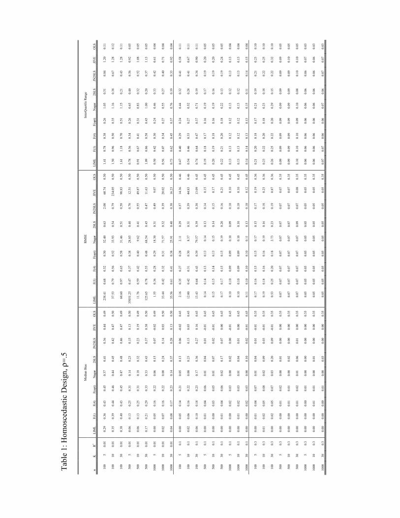
considered to be weak instrument situations. Our results, which are reported in Tables 1 - 5,

are based on 5000 replications.

10

In order to highlight the weak instrument nature of our simulation design we compare it

to parametrizations typically used in the exact Þnite sample distribution literature for LIML

and 2SLS. In particular consider the parametrization in Anderson, Kunitomo and Sawa (1982).

They deÞne

δ2 =π0 (Pni=1 ziz

0i)π

ω22

and

α =ω22

|Ω|1/2µβ − ω12

ω22

¶where the reduced form covariance matrix is given by

Ω =

"ω11 ω12

ω21 ω22

#=

"σ11 + 2βσ12 + β

2σ22 σ12 + βσ22

σ12 − βσ22 σ22

#for the structural errors [εi, ui] N(0,Σ) and Σ with elements σij. Given our assumption about

zi it follows at once that δ2 ≈ n·π0π = n·q ·η2. This implies that δ2 ≈ nR2/¡1−R2¢ and we also

Þnd that α = −ρ/p1− ρ2 or ρ = −α/√1 + α2. We compute values of δ for the parametrizations

that we use in our simulations. The results are summarized in Table 7.

4.3 Monte Carlo Results

4.3.1 Median Bias

We Þrst consider the median bias results. Especially for the situation of R2 = 0.01 the absence

of Þnite sample moments for LIML, Nagar, and JIVE is apparent. Among the three Fuller

estimators, F(1) has the smallest bias, in accordance with the second order theory. Also, the

median bias increases as we go to F(4) and F(opt), again as theory predicts. When R2 increases

to 0.1 the F(1) estimator often does better than JN2SLS, but not by large amounts. Lastly, when

R2 increases to 0.3, the Þnite sample problem ceases to be important, and LIML, Nagar and

the other estimators do well. We conclude that for sample sizes above 100 that R2=0.3 is high

enough that Þnite sample problems cease to be a concern. Overall, the JN2SLS estimator does

quite well in terms of bias - it is usually comparable and sometimes smaller than the unbiased

F(1) estimator, although on average F(1) does better than JN2SLS. Overall, JN2SLS has smaller

bias than either the F(4) estimator or the infeasible F(opt) estimator. JN2SLS also has smaller

bias than the 2SLS estimator, as expected. In general, LIML seems to have the smallest median

bias, at least under homoscedastic design. This is in agreement with the well-known fact that

LIML has a zero higher order median bias. On the other hand, the actual median bias of LIML

is not equal to zero, which can be explained by the alternative asymptotic analysis put forth by

Staiger and Stock (1997). See Section 5.3.

11

4.3.2 MSE

For LIML, F(1), F(4), and F(opt), the approximate MSE is equal to

1−R2nR2

+K1− ρ2n2

µ1−R2R2

¶2+O

µ1

n2

¶(6)

To allow for a more reÞned expression for the MSE of the Fuller estimators, we also calculate

the MSE of F(4) using the approach of Rothenberg (1983):

1−R2nR2

+ ρ2−1−Kn2

µ1−R2R2

¶2+K − 6n2

µ1−R2R2

¶2(7)

For Nagar, JN2SLS, and JIVE, the approximate MSE is equal to

1−R2nR2

+K1 + ρ2

n2

µ1−R2R2

¶2+O

µ1

n2

¶(8)

Thus, note that JN2SLS has the same MSE as Nagar or JIVE, but JN2SLS has Þnite sample

moments as we demonstrated above. For 2SLS, the MSE is equal to

1−R2nR2

+K2 ρ2

n2

µ1−R2R2

¶2+O

µ1

n2

¶(9)

The Þrst order term is identical for all the estimators as is well known. The second order terms

depend on the number of instruments as K and for 2SLS as K2. Note that for 2SLS the second

order term is the square of the bias term of 2SLS from Hahn and Hausman (2001).

When we turn to the empirical results, we Þnd that the theory does not give especially

good guidance to the actual empirical results. Although Nagar is supposed to be equivalent

to JN2SLS, it is not and performs considerably worse than JN2SLS when the model is weakly

identiÞed. Presumably the lack of moments invalidates the Nagar calculations. Indeed we

strongly recommend that the no-moment estimators LIML, Nagar, and JIVE not be used in

weak instrument situations. The ordering of the empirical MSE of the Fuller estimators is in

accord with the higher order theory as discussed by Rothenberg (1983) and in the Appendix C.

If we compare the best of the feasible Fuller estimators F(4) to JN2SLS, the F(4) estimator does

better with a small number of instruments, but JN2SLS often does better when the number of

instrument increases. However, we might give a slight nod to the F(4) estimator over JN2SLS

here. Note that 2SLS turns in a respectable performance here, also.

2SLS tends to dominate OLS in terms of both bias and RMSE except most extreme cases

very small R2.

4.3.3 Interquartile Range (IQR)

We think that the IQR is a useful measure since extreme results do not matter. Thus, a

reasonable conjecture is that the no moment estimators would be superior with respect to

12

the IQR. This is not what we Þnd however. Instead, LIML, Nagar, and JIVE are all found to

have signiÞcantly larger IQR than the other estimators. Since the no-moment estimators also

have inferior empirical mean bias and MSE performance, we suggest that they are not useful

estimators in the weak instrument situation. For the IQR we Þnd that the F(4) estimator does

signiÞcantly better than the F(1) estimator. 2SLS does better than JN2SLS for the IQR, but

often not by large amounts. The F(4) estimator has no ordering with respect to 2SLS and

JN2SLS.

Based on the mean bias, the MSE, and the IQR we Þnd no overall ordering among the 2SLS,

F(4), and JN2SLS estimators. However, these estimators perform better than the no moment

estimators. We suggest that the Fuller estimator receive more attention and use than it seems to

have received to date. We also suggest that the 2SLS estimator and the JN2SLS be calculated

in a weak instrument situation. These three estimators seem to have the best properties of the

estimators we investigated. Overall, our Þnding is that 2SLS does better than would be expected

based on the theoretical calculations.

4.3.4 A Heteroscedastic Design

We now consider a heteroscedastic design where E£ε2i¯zi¤= z0izi/K. We only consider F(4),

2SLS, and JN2SLS because the no-moment estimators continue to have similar problems

as in the homoscedastic case. We Þnd that in terms of mean bias that JN2SLS does better

than either F(4) or 2SLS. For MSE, F(4) often does better than JN2SLS, but also often does

considerably worse. 2SLS often does better than JN2SLS. Based on the MSE we thus again

suggest considering all three estimators. Our suggested use of all three estimators remains the

same based on IQR. Thus, the use of a heteroscedastic design continues to lead to the same

suggestion as the homoscedastic design.

4.3.5 How Important are Outliers?

In Table 5 we analyze the importance of outliers by comparing the 5−95% range of the empiricaldistribution of our estimators to the range implied by the asymptotic distribution. The table

shows that the no-moment estimators, LIML, Nagar and Jive, have severely inßated ranges rela-

tive to their asymptotic distribution when R2 = 0.01. This suggests that for the weak instrument

case the nonexistence of moments affects the entire distribution and is not a feature of extreme

tail behavior alone. On the other hand, the estimators with known Þnite moments, Fuller,

2SLS and JN2SLS do not show inter quantile ranges larger than predicted by the asymptotic

distribution.

13

5 How Well Do the Higher Order Formulae Explain the Data?

All of our bias and MSE formula are higher order asymptotic expansions to O¡1/n2

¢. We have

already ascertained that for the no-moment estimators the formulae are not useful in the weak

instrument situation. More generally, we have determined above from the Monte Carlo results

that the asymptotic expansions may not provide especially good guidance in the weak instrument

situation. Thus, we now test the asymptotic expansions given the data obtained from the Monte

Carlo experiments. We consider the formulae in two respects. We Þrst take the MSE formulae

given above and run a regression, using our Monte Carlo design results, of the empirical MSE

on the theory predictions. We use a constant, which should be zero, and an intercept, which

should be one, if the formulae hold true. We then alternatively run a regression using the Þrst

and second order terms separately from the MSE formulae. Each of the coefficients should be

unity. This latter approach allows us to sort out the Þrst and second order terms.

5.1 Basic Regression Results

We Þrst run the 0-1 regression with a constant and a coefficient for the MSE formulae that we

derived for the estimators. The results should be the constant=0 and the intercept coefficient

=1 if the formulae are correct for our Monte Carlo weak instrument design. The results are

given in Table 8.

Even for the estimators with Þnite sample moments, the higher formulae are all rejected

since none of the intercepts equals anywhere near unity. The JN2SLS, Fuller (4) and 2SLS have

some predictive power.

5.2 Further Regression Results

We now repeat the regressions, but we separate the RHS into the two terms corresponding to

the Þrst order and second order terms in the approximate MSE formulae. The Þrst term with

coefficient C1 is the Þrst order term while the next term with coefficient C2 is the second order

term: We present the results in Table 9.

All the coefficients should be unity if the formulae are correct. None of the estimates are

unity. The Þrst order terms are most important, as expected. The second order terms are

typically small in magnitude, but often signiÞcant. However, the signs of the second order

coefficients for JN2SLS and F(4) are incorrect while the second order coefficient for 2SLS is very

small and not signiÞcant. The Þt of the regression is improved by dividing up the terms. Thus,

the second order terms do not do a good job in explaining the empirical results.

14

5.3 Numerical Calculation of the Median of the Weak Instrument Limit Dis-tribution of LIML

Our Monte Carlo result can be related to the alternative asymptotic analysis put forth by Staiger

and Stock (1997). Under their alternative approximation, our model is such that

yi = xiβ + εi, xi = z0iπ + ui

where zi ∼ N (0, IK), vi = (εi, ui)0 with vi ∼ N (0,Σ) and

Σ =

Ã1 ρ

ρ 1

!,

π = (η, ..., η)0 /√n for some constant η. DeÞne λ =

√n (η, ..., η)0, and let eφ be the smallest

eigenvalue of the matrix W 0W (W 0MW )−1. Denote by φ the limit of n³eφ− 1´ . As in Staiger

and Stock (1997), we may then assume that³n³eφ− 1´ , n−1/2Z0ε, n−1/2Z0u´⇒ ¡

φ,ΨZε,ΨZu¢,

where ΨZε,ΨZu have a marginal normal distribution (ΨZε,ΨZu)0 ∼ N (0,Σ⊗ Ik). The limiting

distribution of the LIML estimator under local to zero asymptotics then is deÞned by letting

v1 = (λ+ΨZu)0 (λ+ΨZu) and v2 = (λ+ΨZu)0ΨZε, where λ = (η, ..., η)0. As Staiger and Stock

(1997) show,

βLIML − β ⇒¡v2 − φρ

¢/¡v1 − φ

¢.

We draw samples from the distribution of (v2 − κρ) / (v1 − κ) by generating y, x, Z according to(1) for sample sizes n = (100, 500, 1000). We chose r = .01, .1, .3 and K = 5, 10, 30. We use³n³eφ− 1´ , n−1/2Z 0ε, n−1/2Z 0u´ as an approximation to ¡φ,ΨZε,ΨZu¢ and computeβ∗i =

¡λ+ n−1/2Z0u

¢0n−1/2Z 0ε− n (k − 1) ρ¡

λ+ n−1/2Z 0u¢0 ¡λ+ n−1/2Z0u

¢− n (k − 1)for each Monte Carlo replication. We compute the median of the empirical distribution of

β∗i , i = 1, ...., S as an approximation to the median of¡v2 − φρ

¢/¡v1 − φ

¢. The results for

10,000 replications are summarized in Table 11. The simulation results indicate that the ap-

proximation of Staiger and Stock (1997) implies the presence of a median bias for LIML when

the concentration parameter λ is small. In those instances the median bias is also an increasing

function of the number of instruments K. The numerical evaluation of the Staiger and Stock

(1997) local to zero approximation is quite close to the actual Þnite sample distribution of LIML

obtained by Monte Carlo procedures as far as median bias properties are concerned.

15

5.4 An Empirical Exploration

Our last set of empirical analysis consists of regressing the log of the MSE on the logs of the

determinants of the MSE: n, K, ρ, and 1−R2R2

= Ratio. The results are given in Table 10.

The effects of the number or observations n and R2 have the expected magnitude and are

estimated quite precisely-the Þrst order effect dominates as we would expect. However, the

second order effects of the correlation coefficient (squared) and the number of instruments are

considerably less important. While the number of instruments is most important for 2SLS as

the second order MSE formulae predict, the estimated coefficient is far below 2.0, which is the

theoretical prediction. Perhaps the most important Þnding is that the effect of the number of

instruments is considerably less than expected. Thus, number of instruments pessimism that

arises from the second order formulae on the asymptotic bias seems to be overdone. This Þnding

is consistent with our results that 2SLS does better than expected in many situations.

Lastly, we run a regression with the same RHS variables as controls but with the LHS side

variable the log of MSE and additional RHS variables as indicator variables. Thus, we run a

horse race among the different estimators. For the log of MSE estimators we Þnd the no

moments estimators to have signiÞcantly higher log MSE than the baseline estimator, 2SLS.

We Þnd 2SLS signiÞcantly better than all of the other estimators except JN2SLS. JN2SLS has

a smaller log MSE than 2SLS. Both estimators are signiÞcantly better than Fuller (4) which,

in turn, is signiÞcantly better than the no moments estimators. For log IQR we Þnd that

2SLS is insigniÞcantly better than F(4), which in turn is insigniÞcantly better than JN2SLS. No

signiÞcant difference exist for the three estimators with respect to log IQR. The no moments

estimators do signiÞcantly worse than these three estimators. Thus, the choice of estimator may

depend on whether the researcher is interested more in the entire distribution as given by the

MSE or in the IQR. The overall Þnding is that the F(4) and JN2SLS should be used along with

2SLS in the weak instruments situation.

16

Appendix

A Higher Order Expansion

We Þrst present two Lemmas:

Lemma 1 Let υi be a sample of n independent random variables with maxiE [|υi|r] < cr <∞for some constant 0 < c <∞ and some 1 < r <∞. Then maxi |υi| = Op

¡n1/r

¢.

Proof. By Jensens inequality, we have

E

·maxi|υi|¸≤µE

·maxi|υi|r

¸¶1/r≤ÃX

i

E [|υi|r]!1/r

≤µnmax

iE [|υi|r]

¶1/r= n1/r

µmaxiE [|υi|r]

¶1/r≤ n1/rc

The conclusion follows by Markov inequality.

Lemma 2 Assume that Conditions 2 and 3 are satisÞed. Further assume that E [|εi|r] < ∞and E [|ui|r] <∞ for r sufficiently large (r > 12). We then have (i) n−1/6max |δ1i| = op (1) andn−1/6max |δ2i| = op (1); and (ii) 1

n√n

Pi

¯δ1iδ

22i

¯= op (1) and 1

n√n

Pi

¯δ32i¯= op (1).

Proof. Note that

max |δ1i| ≤ (max |fi|+max |ui|) ·max |εi|+max (1− Pii)−1 · (max |ui|+max |(Pu)i|) · (max |εi|+max |(Pε)i|) ,

We have (max |fi|+max |ui|) · max |εi| = Op¡n2/r

¢by Lemma 1. Because max |(Pu)i|2 ≤

maxPii · u0u, and maxPii = O¡1n

¢, we also have max |(Pu)i| = Op (1). Similarly, max |(Pε)i| =

Op (1). Therefore, we obtain we obtain max |δ1i| = op¡n1/6

¢. That max |δ2i| = op

¡n1/6

¢can

be established similarly. It then easily follows that 1n√n

Pi

¯δ1iδ

22i

¯ ≤ 1√nmax |δ1i|max |δ2i|2 =

op (1), and 1n√n

Pi

¯δ32i¯ ≤ 1√

nmax |δ2i|3 = op (1).

We note from Donald and Newey (2001) that we have the following expansion7:

H√nx0Pεx0Px

=7Xj=1

Tj + op

µK

n

¶, (10)

7Our representation of Donald and Neweys result reßects our simplifying assumption that the Þrst stage is

correctly speciÞed.

18

where

T1 = h = Op (1) , T2 =W1 = Op

µK√n

¶, T3 = −W3

1

Hh = Op

µ1√n

¶,

T4 = 0, T5 = −W41

Hh = Op

µK

n

¶, T6 = −W3

1

HW1 = Op

µK

n

¶,

T7 =W23

1

H2h = Op

µ1

n

¶,

and

h =f 0ε√n= Op (1) , W1 =

u0Pε√n= Op

µK√n

¶,

W3 = 2f 0un= Op

µ1√n

¶, W4 =

u0Pun

= Op

µK

n

¶.

We now expand H1nx0Px and

³H

1nx0Px

´2up to Op

¡1n

¢. Because 1

nx0Px = H +W3 +W4, we

haveH

1nx

0Px=

H

H +W3 +W4= 1− 1

HW3 − 1

HW4 +

1

H2W 23 + op

µK

n

¶, (11)Ã

H1nx

0Px

!2= 1− 2 1

HW3 − 2 1

HW4 + 3

1

H2W 23 + op

µK

n

¶(12)

We now expand 1√n

Pi δ1i. Observe that

1√n

Xi

δ1i = − 1√n

Xi

xiεi +1√n

Xi

(1− Pii)−1 (Mx)i (Mε)i

= −h− 1√nu0ε+

1√n(Mu)0

³I − eP´−1 (Mε)

= −h− 1√nu0ε+

1√nu0Mε+

1√n(Mu)0 P (Mε)

= −h− 1√nu0Pε+

1√nu0Pε− 1√

nu0PPε− 1√

nu0PPε+

1√nu0PPPε

= −h− 1√nu0C0ε− 1√

nu0PPε+

1√nu0PPPε, (13)

where, as in Donald and Newey (2001), we let

C ≡ P − P (I − P ) = P − PM, P ≡ eP ³I − eP´−1 ,and eP is a diagonal matrix with element Pii on the diagonal. Now, note that, by Cauchy-

Schwartz,¯u0PPε

¯ ≤ √u0upε0PP 2Pε. Because u0u = Op (n), and ε0PP 2Pε ≤ max³ Pii1−Pii

´2ε0Pε =

O¡1n2

¢Op (K), we obtain¯u0PPε√

n

¯≤ 1√

n

√u0uqε0PP 2Pε =

1√n

qOp (n)

sO

µ1

n2

¶Op (K) = Op

Ã√K

n

!,

¯u0PPPε√

n

¯≤ 1√

n

√u0Pu

qε0PP 2Pε =

1√n

qOp (K)

sO

µ1

n2

¶Op (K) = Op

µK

n3/2

¶= op

µK

n

¶.

19

To conclude, we can write

1√n

Xi

δ1i = −h+W5 +W6 + op

µK

n

¶, (14)

where

W5 ≡ − 1√nu0C0ε = Op

Ã√K√n

!

W6 ≡ 1√nu0PPε = Op

Ã√K

n

!.

We now expand³

H1nx0Px

´³1√n

Pi δ1i

´using (11) and (14):Ã

H1nx

0Px

!Ã1√n

Xi

δ1i

!

=

µ1− 1

HW3 − 1

HW4 +

1

H2W 23

¶(−h+W5 +W6) + op

µK

n

¶= −h+W3

1

Hh+W4

1

Hh−W 2

3

1

H2h+W5 +W6 − 1

HW3W5 + op

µK

n

¶= −T1 − T3 − T5 − T7 + T8 + T9 + T10 + op

µK

n

¶(15)

where

T8 ≡ W5 = − 1√nu0C0ε = Op

Ã√K√n

!,

T9 ≡ W6 =1√nu0PPε = Op

Ã√K

n

!,

T10 ≡ − 1HW3W5 =W3

1

H

1√nu0C0ε = Op

Ã√K

n

!.

We now expand H1nx0Px

µ1√nx0P ε

1nx0Px

¶¡1n

Pi δ2i

¢. We begin with expansion of 1n

Pi δ2i. As in

(13), we can show that

1

n

Xi

δ2i = −H − 2

nf 0u− 1

nu0C0u− 1

nu0PPu+

1

nu0PPPu

Because¯u0PPPu

¯ ≤ max

µPii

1− Pii

¶· u0Pu = Op

µK

n

¶,

¯u0PPu

¯ ≤√u0uqu0PP 2Pu ≤

qOp (n)

smax

µPii

1− Pii

¶2· u0Pu = Op

ÃrK

n

!,

20

we may write

1

n

Xi

δ2i = −H −W3 −W7 + op

µK

n

¶(16)

where

W7 ≡ 1

nu0C0u = Op

Ã√K

n

!.

Combining (11) and (16), we obtain

H1nx

0Px

Ã1

n

Xi

δ2i

!=

µ1− 1

HW3 − 1

HW4 +

1

H2W 23

¶(−H −W3 −W7) + op

µK

n

¶= −H +W3 +W4 − 1

HW 23 −W3 +

1

HW 23 −W7 + op

µK

n

¶= −H +W4 −W7 + op

µK

n

¶which, combined with (10), yields

H1nx

0Px

Ã 1√nx0Pε

1nx

0Px

!Ã1

n

Xi

δ2i

!=

1

H

7Xj=1

Tj

(−H +W4 −W7) + op

µK

n

¶

= −7Xj=1

Tj +W41

Hh−W7

1

Hh+ op

µK

n

¶

= −7Xj=1

Tj − T5 + T11 + opµK

n

¶(17)

where

T11 ≡ −W71

Hh = Op

Ã√K

n

!.

We now examine 1H

³H

1nx0Px

´2 ³1

n√n

Pi δ1iδ2i

´. Later in Section B.2.1, it is shown that

1

n√n

Xi

δ1iδ2i = Op

µ1√n

¶Therefore, we should have

1

H

ÃH

1nx

0Px

!2Ã1

n√n

Xi

δ1iδ2i

!= T12 + op

µK

n

¶(18)

where

T12 ≡ 1

H

1

n√n

Xi

δ1iδ2i = Op

µ1√n

¶

21

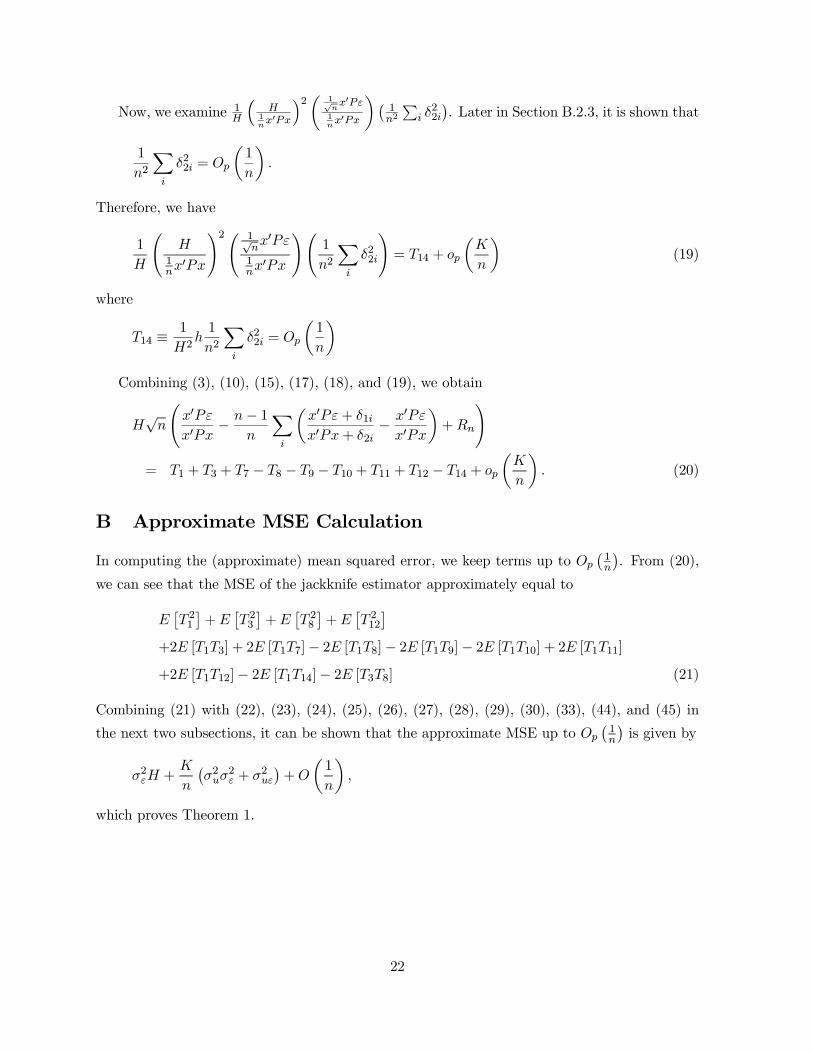
Now, we examine 1H

³H

1nx0Px

´2µ 1√nx0P ε

1nx0Px

¶¡1n2Pi δ22i

¢. Later in Section B.2.3, it is shown that

1

n2

Xi

δ22i = Op

µ1

n

¶.

Therefore, we have

1

H

ÃH

1nx

0Px

!2Ã 1√nx0Pε

1nx

0Px

!Ã1

n2

Xi

δ22i

!= T14 + op

µK

n

¶(19)

where

T14 ≡ 1

H2h1

n2

Xi

δ22i = Op

µ1

n

¶Combining (3), (10), (15), (17), (18), and (19), we obtain

H√n

Ãx0Pεx0Px

− n− 1n

Xi


− x0Pεx0Px

¶+Rn

!

= T1 + T3 + T7 − T8 − T9 − T10 + T11 + T12 − T14 + opµK

n

¶. (20)

B Approximate MSE Calculation

In computing the (approximate) mean squared error, we keep terms up to Op¡1n

¢. From (20),

we can see that the MSE of the jackknife estimator approximately equal to

E£T 21¤+E

£T 23¤+E

£T 28¤+E

£T 212¤

+2E [T1T3] + 2E [T1T7]− 2E [T1T8]− 2E [T1T9]− 2E [T1T10] + 2E [T1T11]+2E [T1T12]− 2E [T1T14]− 2E [T3T8] (21)

Combining (21) with (22), (23), (24), (25), (26), (27), (28), (29), (30), (33), (44), and (45) in

the next two subsections, it can be shown that the approximate MSE up to Op¡1n

¢is given by

σ2εH +K

n

¡σ2uσ

2ε + σ

2uε

¢+O

µ1

n

¶,

which proves Theorem 1.

22

B.1 Approximate MSE Calculation: Intermediate Results That Only Re-quire Symmetry

From Donald and Newey (2001), we can see that

E£T 21¤= σ2εH (22)

E£T 23¤=

4

n

¡σ2uσ

2ε + 2σ

2uε

¢+ o

µ1

n

¶(23)

E [T1T3] = 0 (24)

E [T1T7] =4

n

¡σ2uσ

2ε + 2σ

2uε

¢+ o

µ1

n

¶(25)

E£T 28¤=

K

n

¡σ2uσ

2ε + σ

2uε

¢+ o

µK

nsupPii

¶(26)

Also, by symmetry, we have

E [T1T8] = 0 (27)

E [T1T9] = 0. (28)

It remains to compute E£T 212¤, E [T1T10], E [T1T11], E [T1T12], E [T1T14], and E [T3T8]. We will

take care of E£T 212¤, E [T1T12], and E [T1T14] in the next section.

Note that

E [T1T10] = E [T3T8] = E

·2f 0un

1

H

1√nu0C 0ε

f 0ε√n

¸=

2

n2HE£u0f 0fε · u0C0ε¤

Using equation (18) of Donald and Newey (2001), we obtain

E£u0f 0fε · u0C 0ε¤ =

nXi=1

E£u2i ε

2i f2i C

0ii

¤+

nXi=1

Xj 6=iE£uiεiujεjf

2i C

0jj

¤+

nXi=1

Xj 6=iE£u2i ε

2jfifjC

0ij

¤+

nXi=1

Xj 6=iE£uiεjujεififjC

0ji

¤= σ2uσ

2ε

nXi=1

Xj 6=ififjC

0ij + σ

2uε

nXi=1

Xj 6=ififjC

0ji

= σ2uσ2εf0C 0f + σ2uεf

0Cf

Therefore, we have

E [T1T10] = E [T3T8] =2

nH

σ2uσ2εf0C0f + σ2uεf 0Cf

n

=2

nH

µσ2uσ

2εH + σ

2uεH + o

µ1

n

¶¶=2

n

¡σ2uσ

2ε + σ

2uε

¢+ o

µ1

n2

¶, (29)

where the second equality is based on equation (20) of Donald and Newey (2001).

23

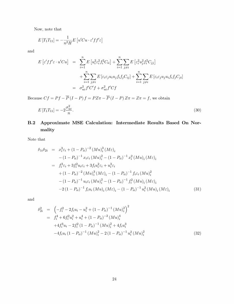
Now, note that

E [T1T11] = − 1

n2HE£u0Cu · ε0ff 0ε¤

and

E£ε0ff 0ε · u0Cu¤ =

nXi=1

E£u2i ε

2i f2i Cii

¤+

nXi=1

Xj 6=iE£ε2i u

2jf2i Cjj

¤+

nXi=1

Xj 6=iE [εiεjuiujfifjCij ] +

nXi=1

Xj 6=iE [εiεjujuififjCji]

= σ2uεf0C 0f + σ2uεf

0Cf

Because Cf = Pf − P (I − P ) f = PZπ − P (I − P )Zπ = Zπ = f , we obtain

E [T1T11] = −2σ2uε

n. (30)

B.2 Approximate MSE Calculation: Intermediate Results Based On Nor-mality

Note that

δ1iδ2i = x3i εi + (1− Pii)−2 (Mu)3i (Mε)i− (1− Pii)−1 xiεi (Mu)2i − (1− Pii)−1 x2i (Mu)i (Mε)i

= f3i εi + 3f2i uiεi + 3fiu

2i εi + u

3i εi

+(1− Pii)−2 (Mu)3i (Mε)i − (1− Pii)−1 fiεi (Mu)2i− (1− Pii)−1 uiεi (Mu)2i − (1− Pii)−1 f2i (Mu)i (Mε)i−2 (1− Pii)−1 fiui (Mu)i (Mε)i − (1− Pii)−1 u2i (Mu)i (Mε)i (31)

and

δ22i =³−f2i − 2fiui − u2i + (1− Pii)−1 (Mu)2i

´2= f4i + 6f

2i u

2i + u

4i + (1− Pii)−2 (Mu)4i

+4f3i ui − 2f2i (1− Pii)−1 (Mu)2i + 4fiu3i−4fiui (1− Pii)−1 (Mu)2i − 2 (1− Pii)−1 u2i (Mu)2i (32)

24

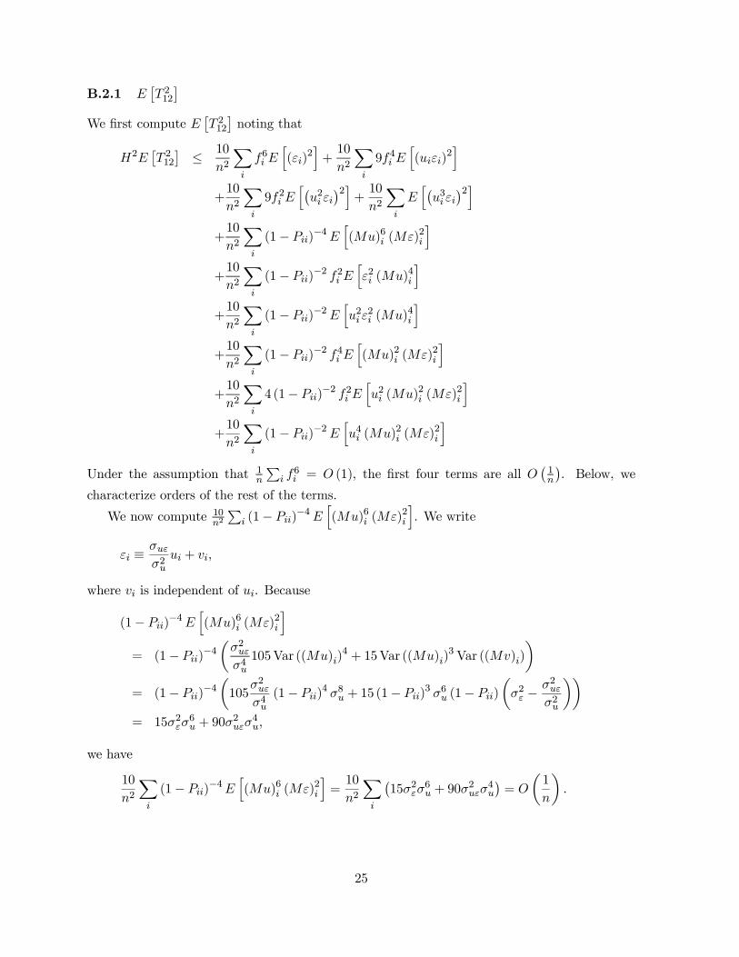
B.2.1 E£T 212¤

We Þrst compute E£T 212¤noting that

H2E£T 212¤ ≤ 10

n2

Xi

f6i Eh(εi)

2i+10

n2

Xi

9f4i Eh(uiεi)

2i

+10

n2

Xi

9f2i Eh¡u2i εi

¢2i+10

n2

Xi

Eh¡u3i εi

¢2i+10

n2

Xi

(1− Pii)−4Eh(Mu)6i (Mε)

2i

i+10

n2

Xi

(1− Pii)−2 f2i Ehε2i (Mu)

4i

i+10

n2

Xi

(1− Pii)−2Ehu2i ε

2i (Mu)

4i

i+10

n2

Xi

(1− Pii)−2 f4i Eh(Mu)2i (Mε)

2i

i+10

n2

Xi

4 (1− Pii)−2 f2i Ehu2i (Mu)

2i (Mε)

2i

i+10

n2

Xi

(1− Pii)−2Ehu4i (Mu)

2i (Mε)

2i

iUnder the assumption that 1

n

Pi f6i = O (1), the Þrst four terms are all O

¡1n

¢. Below, we

characterize orders of the rest of the terms.

We now compute 10n2Pi (1− Pii)−4E

h(Mu)6i (Mε)

2i

i. We write

εi ≡ σuεσ2uui + vi,

where vi is independent of ui. Because


2i

i= (1− Pii)−4

µσ2uεσ4u105Var ((Mu)i)

4 + 15Var ((Mu)i)3Var ((Mv)i)

¶= (1− Pii)−4

µ105

σ2uεσ4u

(1− Pii)4 σ8u + 15 (1− Pii)3 σ6u (1− Pii)µσ2ε −

σ2uεσ2u

¶¶= 15σ2εσ

6u + 90σ

2uεσ

4u,

we have

10

n2

Xi


2i

i=10

n2

Xi

¡15σ2εσ

6u + 90σ

2uεσ

4u

¢= O

µ1

n

¶.

25

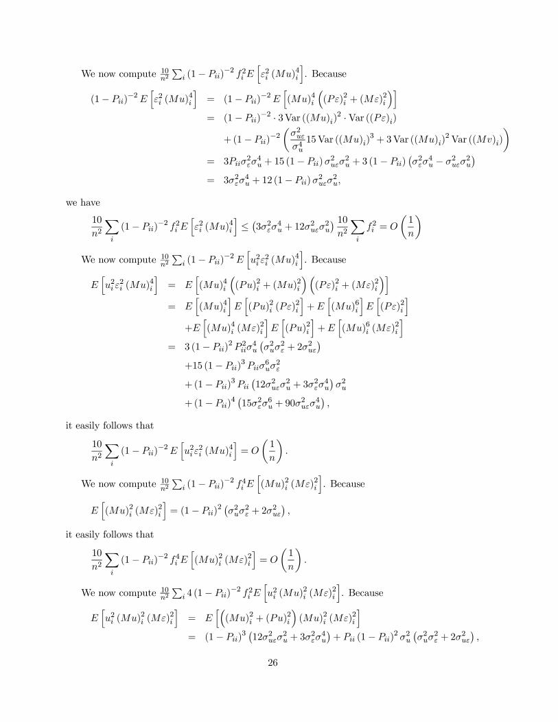
We now compute 10n2Pi (1− Pii)−2 f2i E

hε2i (Mu)

4i

i. Because

(1− Pii)−2Ehε2i (Mu)

4i

i= (1− Pii)−2E

h(Mu)4i

³(Pε)2i + (Mε)

2i

´i= (1− Pii)−2 · 3Var ((Mu)i)2 ·Var ((Pε)i)

+ (1− Pii)−2µσ2uεσ4u15Var ((Mu)i)

3 + 3Var ((Mu)i)2Var ((Mv)i)

¶= 3Piiσ

2εσ4u + 15 (1− Pii)σ2uεσ2u + 3 (1− Pii)

¡σ2εσ

4u − σ2uεσ2u

¢= 3σ2εσ

4u + 12 (1− Pii)σ2uεσ2u,

we have

10

n2

Xi

(1− Pii)−2 f2i Ehε2i (Mu)

4i

i≤ ¡3σ2εσ4u + 12σ2uεσ2u¢ 10n2X

i

f2i = O

µ1

n

¶

We now compute 10n2Pi (1− Pii)−2E

hu2i ε

2i (Mu)

4i

i. Because

Ehu2i ε

2i (Mu)

4i

i= E

h(Mu)4i

³(Pu)2i + (Mu)

2i

´³(Pε)2i + (Mε)

2i

´i= E

h(Mu)4i

iEh(Pu)2i (Pε)

2i

i+E

h(Mu)6i

iEh(Pε)2i

i+E

h(Mu)4i (Mε)

2i

iEh(Pu)2i

i+E

h(Mu)6i (Mε)

2i

i= 3 (1− Pii)2 P 2iiσ4u

¡σ2uσ

2ε + 2σ

2uε

¢+15 (1− Pii)3 Piiσ6uσ2ε+(1− Pii)3 Pii

¡12σ2uεσ

2u + 3σ

2εσ4u

¢σ2u

+(1− Pii)4¡15σ2εσ

6u + 90σ

2uεσ

4u

¢,

it easily follows that

10

n2

Xi

(1− Pii)−2Ehu2i ε

2i (Mu)

4i

i= O

µ1

n

¶.

We now compute 10n2Pi (1− Pii)−2 f4i E

h(Mu)2i (Mε)

2i

i. Because

Eh(Mu)2i (Mε)

2i

i= (1− Pii)2

¡σ2uσ

2ε + 2σ

2uε

¢,


10

n2

Xi

(1− Pii)−2 f4i Eh(Mu)2i (Mε)

2i

i= O

µ1

n

¶.

We now compute 10n2Pi 4 (1− Pii)−2 f2i E

hu2i (Mu)

2i (Mε)

2i

i. Because

Ehu2i (Mu)

2i (Mε)

2i

i= E

h³(Mu)2i + (Pu)

2i

´(Mu)2i (Mε)

2i

i= (1− Pii)3

¡12σ2uεσ

2u + 3σ

2εσ4u

¢+ Pii (1− Pii)2 σ2u

¡σ2uσ

2ε + 2σ

2uε

¢,

26


10

n2

Xi

4 (1− Pii)−2 f2i Ehu2i (Mu)

2i (Mε)

2i

i=

¡12σ2uεσ

2u + 3σ

2εσ4u

¢ 40n2

Xi

f2i (1− Pii) + σ2u¡σ2uσ

2ε + 2σ

2uε

¢ 40n2

Xi

f2i Pii (1− Pii)2

= O

µ1

n

¶.

We Þnally compute 10n2Pi (1− Pii)−2E

hu4i (Mu)

2i (Mε)

2i

i. Because

Ehu4i (Mu)

2i (Mε)

2i

i= E

h³(Mu)4i + 2 (Mu)

2i (Pu)

2i + (Pu)

4i

´(Mu)2i (Mε)

2i

i= E

h(Mu)6i (Mε)

2i

i+ 2E

h(Pu)2i

iEh(Mu)4i (Mε)

2i

i+E

h(Pu)4i

iEh(Mu)2i (Mε)

2i

i= (1− Pii)4

¡15σ2εσ

6u + 90σ

2uεσ

4u

¢+ 2Pii (1− Pii)3 σ2u

¡12σ2uεσ

2u + 3σ

2εσ4u

¢+3P 2ii (1− Pii)2 σ4u

¡σ2uσ

2ε + 2σ

2uε

¢,


10

n2

Xi

(1− Pii)−2Ehu4i (Mu)

2i (Mε)

2i

i= O

µ1

n

¶.

To summarize, we have

E£T 212¤= O

µ1

n

¶. (33)

B.2.2 E [T1T12]

We now compute E [T1T12]. We compute the expectation of the product of each term on the

right side of (31) with f 0ε.

E£¡f 0ε¢ ¡f3i εi

¢¤= f4i σ

2ε (34)

E£¡f 0ε¢ ¡3f2i uiεi

¢¤= 0 (35)

E£¡f 0ε¢ ¡3fiu

2i εi¢¤

= 3f2i¡σ2uσ

2ε + 2σ

2uε

¢(36)

E£¡f 0ε¢ ¡u3i εi

¢¤= 0 (37)

Now note that

E£Mu

¡f 0u¢¤

= σ2uMf = 0, E£Mu

¡f 0ε¢¤= σuεMf = 0,

E£Mε

¡f 0u¢¤

= σuεMf = 0, E£Mε

¡f 0ε¢¤= σ2εMf = 0,

27

which implies independence. Therefore, we have

Eh¡f 0ε¢ · (1− Pii)−2 (Mu)3i (Mε)ii = 0 (38)

Lemma 3 Suppose that A,B,C are zero mean normal random variables. Also suppose that A

and B are independent of each other. Then E£A2BC

¤= Cov (B,C)Var (A).

Proof. Write

C =Cov (A,C)

Var (A)A+

Cov (B,C)

Var (B)B + v

where v is independent of A and B. Conclusion easily follows.

Using Lemma 3, we obtain

Eh¡f 0ε¢ · ³− (1− Pii)−1 fiεi (Mu)2ií = − (1− Pii)−1Cov

¡f 0ε, fiεi

¢Var ((Mu)i)

= − (1− Pii)−1 f2i σ2ε (1− Pii)σ2u= −f2i σ2εσ2u (39)

Symmetry implies

Eh¡f 0ε¢ · ³− (1− Pii)−1 uiεi (Mu)2ií = 0 (40)

and

Eh¡f 0ε¢ · ³− (1− Pii)−1 f2i (Mu)i (Mε)ií = 0 (41)

Lemma 4 Suppose that A,B,C,D are zero mean normal random variables. Also suppose that

(A,B) and C are independent of each other. Then E [ABCD] = Cov (A,B)Cov (C,D)

Proof. Write D = ξ1A+ ξ2B + ξ3C + v, where ξs denote regression coefficients. Note that

ξ3 = Cov (C,D) /Var (C) by independence. We then have

ABCD = ξ1A2BC + ξ2AB

2C + ξ3ABC2 +ABCv

from which the conclusion follows.

Using Lemma 4, we obtain

Eh¡f 0ε¢ · ³−2 (1− Pii)−1 fiui (Mu)i (Mε)ií

= −2 (1− Pii)−1Cov ((Mu)i , (Mε)i)Cov¡f 0ε, fiui

¢= −2 (1− Pii)−1 (1− Pii)σuεf2i σuε= −2σ2uεf2i (42)

28

Finally, using symmetry again, we obtain

Eh¡f 0ε¢ · ³− (1− Pii)−1 u2i (Mu)i (Mε)i´i = 0 (43)

Combining (34) - (43), we obtain

E£¡f 0ε¢ · (δ1iδ2i)¤ = f4i σ2ε + 2f2i ¡σ2uσ2ε + 2σ2uε¢ ,

from which we obtain

E [T1T12] =1

H

1

n2

Xi

E£¡f 0ε¢ · (δ1iδ2i)¤ = 1

n

σ2εH

Ã1

n

Xi

f4i

!+ 2

σ2uσ2ε + 2σ

2uε

n. (44)

B.2.3 1n2Pni=1 δ

22i

We compute E£1n2Pni=1 δ

22i

¤and characterize its order of magnitude. From (32), we can obtain

E£δ22i¤= f4i + 4f

2i σ

2u + 4Piiσ

4u,

and hence, it follows that

E

"1

n2

nXi=1

δ22i

#=1

n

Ã1

n

nXi=1

f4i

!+4Hσ2un

+ o

µK

n

¶.

B.2.4 E [T1T14]

We compute the expectation of the product of each term on the right hand side of (32) with

(f 0ε)2, noting independence between (Mu)i and f0ε. We have

Eh¡f 0ε¢2 · f4i i = f 0fσ2εf4i = nHσ2εf4i ,

Eh¡f 0ε¢2 · 6f2i u2i i = 6f2i

³¡f 0fσ2ε

¢σ2u + 2 (fiσuε)

2´

= 6nHσ2εσ2uf2i + 12σ

2uεf

4i ,

Eh¡f 0ε¢2 · u4i i = 12f2i σ

2uεσ

2u + 3f

0fσ2εσ4u

= 3nHσ2εσ4u + 12f

2i σ

2uεσ

2u,

Eh¡f 0ε¢2 · (1− Pii)−2 (Mu)4i i = ¡f 0fσ2ε¢ · 3σ4u = 3nHσ2εσ2u,

Eh¡f 0ε¢2 · ¡4f3i ui¢i = 0,

29

Eh¡f 0ε¢2 · ³−2f2i (1− Pii)−1 (Mu)2ií = −2f2i f 0fσ2εσ2u = −2nHf2i σ2εσ2u,

Eh¡f 0ε¢2 · ¡4fiu3i ¢i = 0,

Eh¡f 0ε¢2 · ³−4fiui (1− Pii)−1 (Mu)2ií = 0,

Eh¡f 0ε¢2 · ³−2 (1− Pii)−1 u2i (Mu)2ií = −4f2i σ2uεσ2u − 4 (1− Pii)nHσ2εσ4u − 2nHσ2εσ4u.

Therefore,

E

"¡f 0ε¢2 nX

i=1

δ22i

#= n2Hσ2ε

Ã1

n

nXi=1

f4i

!+ 6n2H2σ2εσ

2u + 12nσ

2uε

Ã1

n

nXi=1

f4i

!+3n2Hσ2εσ

2u + 12nHσ

2uεσ

2u + 3n

2Hσ2εσ2u − 2n2H2σ2εσ

2u

−4nHσ2uεσ2u − 4 (n−K)nHσ2εσ4u − 2n2Hσ2εσ4u,

and therefore, we have

E [T1T14] =1

H2n3E

"¡f 0ε¢2 nX

i=1

δ22i

#

=1

n

1

Hσ2ε

Ã1

n

nXi=1

f4i

!+1

n

µ6

Hσ2εσ

2u + 4σ

2εσ2u −

6

Hσ2εσ

4u

¶+ o

µ1

n

¶. (45)

C Higher Order Bias and MSE of Fuller

The results in this section was derived using Donald and Neweys (2001) adaptation of Rothen-

berg (1983). Under the normalization where σ2ε = σ2u = 1 and σεu = ρ, we have the following

result. For F(1), the higher order mean bias and the higher order MSE are equal to

0

and

1−R2nR2

+ ρ2−K + 2

n2

µ1−R2R2

¶2+K

n2

µ1−R2R2

¶2Here, R2 denotes the theoretical R2 as deÞned in (5). For F(4), they are equal to

ρ3

n

1−R2R2

30

and

1−R2nR2

+ ρ2−1−Kn2

µ1−R2R2

¶2+K − 6n2

µ1−R2R2

¶2For Fuller(Optimal), they are equal to

ρ2 + 1

ρ2

n

1−R2R2

and

1−R2nR2

+1

n2

µ¡1− ρ2¢K − 1

ρ2− 2ρ2 − 4

¶µ1−R2R2

¶2

31

References

[1] Akahira, M. (1983), Asymptotic DeÞciency of the Jackknife Estimator, Australian

Journal of Statistics 25, 123 - 129.

[2] Anderson, T.W., K. Morimune and T. Sawa (1983), The Numerical Values of Some

Key Parameters in Econometric Models, Journal of Econometrics 21, 229-243.

[3] Anderson, T.W., N. Kunitomo and T. Sawa (1982), Evaluation of the Distribution

Function of the Limited Information Maximum Likelihood Estimator, Econometrica 50,

1009-1028.

[4] Anderson, T.W. and T. Sawa (1973), Distributions of Estimates of Coefficients of a

Single Equation in a Simultaneous System and Their Asymptotic Expansions, Economet-

rica 41, 683-714.

[5] Anderson, T.W. and T. Sawa (1979), Evaluation of the Distribution Function of the

Two Stage Least Squares Estimator, Econometrica 47, 163 - 182.

[6] Angrist, J.D., G.W. Imbens, and A. Krueger (1995), Jackknife Instrumental Vari-

ables Estimation, NBER Technical Working Paper No. 172.

[7] Angrist, J.D., G.W. Imbens, and A.B. Krueger (1999) Jackknife Instrumental Vari-

ables Estimation, Journal of Applied Econometrics 14, 57 67.

[8] Bekker, P.A. (1994), Alternative Approximations to the Distributions of Instrumental

Variable Estimators, Econometrica 92, 657 681.

[9] Davidson, R., and J.G. MacKinnon (1993), Estimation and Inference in Econometrics,

New York: Oxford University Press.

[10] Donald, S. G. and W. K. Newey (2001), Choosing the Number of Instruments,

Econometrica 69, 1161-1191.

[11] Donald, S.G., and W.K. Newey (2000), A Jackknife Interpretation of the Continuous

Updating Estimator, Economics Letters 67, 239-243.

[12] Fuller, W.A. (1977), Some Properties of a ModiÞcation of the Limited Information

Estimator, Econometrica 45, 939-954.

[13] Hahn, J., and J. Hausman (2002), A New SpeciÞcation Test of the Validity of Instru-

mental Variables, Econometrica 70, 163-189.

32

[14] Hahn, J., and J. Hausman (2001), Notes on Bias in Estimators for Simultaneous Equa-

tion Models, forthcoming in Economics Letters.

[15] Hausman, J. (1983), SpeciÞcation and Estimation of Simultaneous Equation Models, in

Griliches, Z., and M.D. Intriligator eds Handbook of Econometrics, Vol. I. Amster-

dam: Elsevier.

[16] Holly, A., and P.C.B. Phillips (1979), A Saddlepoint Approximation to the Distri-

bution of the k-Class Estimator of a Coefficient in a Simultaneous System, Econometrica

47, 1527-1548.

[17] Kuersteiner, G.M., 2000, Mean Squared Error Reduction for GMM Estimators of Lin-

ear Time Series Models unpulished manuscript.

[18] Maddala, G.S., and J. Jeong (1992), On the Exact Small Sample Distribution of the

Instrumental Variables Estimator, Econometrica 60, 181 - 183.

[19] Mariano, R. S (1972), The Existence of Moments of the Ordinary Least Squares and

Two-Stage Least Squares Estimators, Econometrica 40, 643 - 652.

[20] Mariano, R.S. AND T. Sawa (1972), The Exact Finite-Sample Distribution of the

Limited-Information Maximum Likelihood Estimator in the Case of Two Included Endoge-

nous Variables, Journal of the American Statistical Association 67, 159 163.

[21] Morimune, K. (1983), Approximate Distributions of the k-Class Estimators when the

Degree of OveridentiÞability is Large Compared with the Sample Size, Econometrica 51,

821 - 841.

[22] Nagar, A.L. (1959), The Bias and Moment Matrix of the General k-Class Estimators of

the Parameters in Simultaneous Equations, Econometrica 27, 575 - 595.

[23] Newey, W.K., and R.J. Smith (2001), Higher Order Properties of GMM and General-

ized Empirical Likelihood Estimators, mimeo.

[24] Oberhelman, T.W., and K.R. Kadiyala (1983), Asymptotic Probability Concentra-

tions and Finite Sample Properties of ModiÞed LIML Estimators for Equations with more

than Two Endogenous Variables, Journal of Econometrics 98, 163-185.

[25] Phillips, G.D.A., and C. Hale (1977), The Bias of Instrumental Variable Estimators

of Simultaneous Equation Systems, International Economic Review 18, 219-228.

[26] Phillips, P.C.B. (1980), The Exact Distribution of Instrumental Variable Estimators in

an Equation Containing n+1 Endogenous Variables, Econometrica 48, 861-878.

33

[27] Rothenberg, T.J. (1983), Asymptotic Properties of Some Estimators In Structural Mod-

els, in Studies in Econometrics, Time Series, and Multivariate Statistics.

[28] Rothenberg, T.J. (1984), Approximating the Distributions of Econometric Estimators

and Test Statistics, in Handbook of Econometrics 2, Amsterdam: North-Holland.

[29] Sawa, T. (1972), Finite-Sample Properties of the k-Class Estimators, Econometrica 40,

653-680.

[30] Shao, J., and D. Tu (1995), The Jackknife and Bootstrap. New York: Springer-Verlag.

[31] Staiger, D., and J. Stock (1997), Instrumental Variables Regression with Weak In-

struments, Econometrica 65, 557 - 586.

34

Tabl

e 1:

Hom

osce

dast

ic D

esig

n, ρ

=.5

M

edia

n Bi

as

RMSE

In

terQ

uarti

le R

ange

n K

R2

LIM

L F(

1)

F(4)

F(

opt)

Nag

ar

2SLS

JN

2SLS

JI

VE

OLS

LI

ML

F(1)

F(

4)

F(op

t) N

agar

2S

LS

JN2S

LS

JIV

E O

LS

LIM

L F(

1)

F(4)

F(

opt)

Nag

ar

2SLS

JN

2SLS

JI

VE

OLS

100

5 0.

01

0.29

0.

36

0.43

0.

45

0.37

0.

41

0.36

0.

44

0.49

23

8.41

0.

68

0.52

0.

50

52.4

0 0.

63

2.08

60

.74

0.50

1.

41

0.78

0.

38

0.26

1.

05

0.51

0.

84

1.20

0.

11

100

10

0.01

0.

35

0.39

0.

44

0.46

0.

44

0.45

0.

42

0.47

0.

50

37.5

3 0.

79

0.56

0.

52

33.9

3 0.

54

0.79

23

4.05

0.

50

1.50

0.

96

0.50

0.

35

1.16

0.

38

0.67

1.

28

0.12

100

30

0.01

0.

38

0.40

0.

43

0.45

0.

47

0.48

0.

46

0.47

0.

49

60.6

0 0.

97

0.65

0.

58

31.4

6 0.

51

0.58

98

.83

0.50

1.

61

1.18

0.

70

0.51

1.

15

0.21

0.

43

1.28

0.

11

500

5 0.

01

0.06

0.

13

0.25

0.

31

0.14

0.

23

0.15

0.

13

0.50

35

031.

25

0.47

0.

37

0.38

28

.85

0.40

0.

78

12.5

1 0.

50

0.78

0.

56

0.34

0.

26

0.65

0.

40

0.56

0.

92

0.05

500

10

0.01

0.

06

0.13

0.

25

0.31

0.

18

0.32

0.

23

0.19

0.

49

11.7

6 0.

59

0.42

0.

40

9.62

0.

41

0.55

49

.87

0.50

0.

91

0.67

0.

41

0.31

0.

83

0.32

0.

52

1.08

0.

05

500

30

0.01

0.

17

0.21

0.

29

0.33

0.

33

0.43

0.

37

0.38

0.

50

125.

65

0.78

0.

53

0.48

68

.54

0.45

0.

47

11.6

3 0.

50

1.09

0.

86

0.58

0.

45

1.00

0.

20

0.37

1.

13

0.05

1000

5

0.01

0.

00

0.05

0.

16

0.22

0.

06

0.15

0.

07

-0.0

2 0.

49

1.55

0.

36

0.28

0.

29

18.3

0 0.

31

0.49

9.

07

0.50

0.

50

0.42

0.

30

0.24

0.

46

0.33

0.

42

0.61

0.

04

1000

10

0.

01

0.02

0.

07

0.16

0.

22

0.08

0.

24

0.14

0.

03

0.50

33

.44

0.42

0.

32

0.31

71

.57

0.32

0.

39

20.0

2 0.

50

0.56

0.

47

0.34

0.

27

0.55

0.

27

0.40

0.

71

0.04

1000

30

0.

01

0.04

0.

08

0.17

0.

23

0.14

0.

37

0.28

0.

13

0.50

35

.56

0.61

0.

41

0.38

25

.91

0.40

0.

38

16.2

3 0.

50

0.73

0.

62

0.45

0.

37

0.76

0.

19

0.33

0.

92

0.04

100

5 0.

1 0.

00

0.05

0.

14

0.21

0.

05

0.13

0.

06

-0.0

2 0.

45

2.16

0.

35

0.27

0.

28

2.11

0.

29

0.57

14

.36

0.46

0.

47

0.40

0.

29

0.24

0.

44

0.32

0.

41

0.58

0.

11

100

10

0.1

0.02

0.

06

0.16

0.

22

0.08

0.

23

0.13

0.

03

0.45

12

.00

0.42

0.

31

0.30

8.

37

0.31

0.

39

44.8

3 0.

46

0.54

0.

46

0.33

0.

27

0.52

0.

28

0.41

0.

67

0.11

100

30

0.1

0.06

0.

10

0.18

0.

23

0.17

0.

36

0.27

0.

16

0.45

13

.43

0.64

0.

43

0.39

79

.57

0.39

0.

38

13.0

9 0.

45

0.74

0.

64

0.47

0.

37

0.71

0.

19

0.34

0.

90

0.11

500

5 0.

1 0.

00

0.01

0.

04

0.06

0.

01

0.04

0.

01

-0.0

1 0.

45

0.14

0.

14

0.13

0.

13

0.14

0.

13

0.14

0.

15

0.45

0.

19

0.18

0.

17

0.16

0.

19

0.17

0.

19

0.20

0.

05

500

10

0.1

0.00

0.

00

0.03

0.

05

0.01

0.

07

0.02

-0

.01

0.45

0.

15

0.15

0.

14

0.13

0.

15

0.14

0.

15

0.17

0.

45

0.20

0.

19

0.18

0.

16

0.19

0.

16

0.19

0.

20

0.05

500

30

0.1

0.00

0.

01

0.04

0.

06

0.02

0.

17

0.07

0.

00

0.45

0.

17

0.17

0.

15

0.15

0.

19

0.20

0.

16

0.21

0.

45

0.22

0.

21

0.20

0.

18

0.22

0.

13

0.19

0.

24

0.05

1000

5

0.1

0.00

0.

00

0.02

0.

03

0.00

0.

02

0.00

-0

.01

0.45

0.

10

0.10

0.

09

0.09

0.

10

0.09

0.

10

0.10

0.

45

0.13

0.

13

0.12

0.

12

0.13

0.

12

0.13

0.

13

0.04

1000

10

0.

1 0.

00

0.01

0.

02

0.03

0.

01

0.04

0.

01

0.00

0.

45

0.10

0.

10

0.09

0.

09

0.10

0.

10

0.10

0.

10

0.45

0.

13

0.13

0.

12

0.12

0.

13

0.12

0.

13

0.13

0.

04

1000

30

0.

1 0.

00

0.00

0.

02

0.03

0.

00

0.10

0.

02

-0.0

1 0.

45

0.11

0.

10

0.10

0.

10

0.11

0.

13

0.10

0.

12

0.45

0.

14

0.14

0.

13

0.13

0.

15

0.11

0.

14

0.15

0.

04

100

5 0.

3 0.

00

0.01

0.

04

0.07

0.

01

0.04

0.

01

-0.0

1 0.

35

0.17

0.

16

0.15

0.

15

0.17

0.

15

0.17

0.

19

0.36

0.

21

0.20

0.

18

0.17

0.

21

0.19

0.

21

0.23

0.

10

100

10

0.3

0.01

0.

02

0.05

0.

08

0.02

0.

09

0.03

-0

.01

0.35

0.

19

0.18

0.

16

0.16

0.

19

0.16

0.

18

0.23

0.

36

0.23

0.

22

0.20

0.

18

0.23

0.

18

0.22

0.

25

0.10

100

30

0.3

0.00

0.

02

0.05

0.

07

0.03

0.

20

0.09

-0

.01

0.35

0.

53

0.25

0.

20

0.18

2.

73

0.23

0.

19

0.87

0.

36

0.26

0.

25

0.22

0.

20

0.29

0.

15

0.22

0.

32

0.10

500

5 0.

3 0.

00

0.00

0.

01

0.02

0.

00

0.01

0.

00

0.00

0.

35

0.07

0.

07

0.07

0.

07

0.07

0.

07

0.07

0.

07

0.35

0.

09

0.09

0.

09

0.09

0.

09

0.09

0.

09

0.09

0.

05

500

10

0.3

0.00

0.

00

0.01

0.

01

0.00

0.

02

0.00

0.

00

0.35

0.

07

0.07

0.

07

0.07

0.

07

0.07

0.

07

0.07

0.

35

0.09

0.

09

0.09

0.

09

0.09

0.

09

0.09

0.

10

0.05

500

30

0.3

0.00

0.

00

0.01

0.

02

0.01

0.

06

0.01

0.

00

0.35

0.

07

0.07

0.

07

0.07

0.

07

0.09

0.

07

0.08

0.

35

0.10

0.

10

0.10

0.

09

0.10

0.

08

0.10

0.

10

0.05

1000

5

0.3

0.00

0.

00

0.00

0.

01

0.00

0.

00

0.00

0.

00

0.35

0.

05

0.05

0.

05

0.05

0.

05

0.05

0.

05

0.05

0.

35

0.06

0.

06

0.06

0.

06

0.06

0.

06

0.06

0.

07

0.03

1000

10

0.

3 0.

00

0.00

0.

01

0.01

0.

00

0.01

0.

00

0.00

0.

35

0.05

0.

05

0.05

0.

05

0.05

0.

05

0.05

0.

05

0.35

0.

06

0.06

0.

06

0.06

0.

06

0.06

0.

06

0.06

0.

03

1000

30

0.

3 0.

00

0.00

0.

00

0.01

0.

00

0.03

0.

00

0.00

0.

35

0.05

0.

05

0.05

0.

05

0.05

0.

05

0.05

0.

05

0.35

0.

07

0.07

0.

06

0.06

0.

07

0.06

0.

07

0.07

0.

03

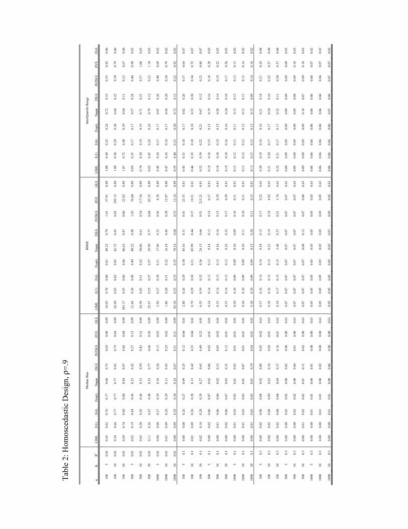
Tabl

e 2:

Hom

osce

dast

ic D

esig

n, ρ

=.9

M

edia

n Bi

as

RMSE

In

terQ

uarti

le R

ange

n K

R2

LIM

L F(

1)

F(4)

F(

opt)

Nag

ar

2SLS

JN

2SLS

JI

VE

OLS

LI

ML

F(1)

F(

4)

F(op

t) N

agar

2S

LS

JN2S

LS

JIV

E O

LS

LIM

L F(

1)

F(4)

F(

opt)

Nag

ar

2SLS

JN

2SLS

JI

VE

OLS

100

5 0.

01

0.43

0.

62

0.76

0.

77

0.68

0.

73

0.65

0.

80

0.89

34

.03

0.78

0.

80

0.81

49

.23

0.79

1.

61

37.9

1 0.

89

1.08

0.

49

0.25

0.

24

0.72

0.

33

0.53

0.

92

0.06

100

10

0.01

0.

54

0.66

0.

77

0.77

0.

77

0.81

0.

75

0.84

0.

89

42.6

9 0.

83

0.82

0.

83

42.7

2 0.

83

0.85

29

5.13

0.

89

1.08

0.

58

0.29

0.

28

0.68

0.

22

0.39

0.

79

0.06

100

30

0.01

0.

69

0.74

0.

80

0.80

0.

84

0.87

0.

84

0.88

0.

89

383.

17

0.93

0.

86

0.86

46

.63

0.87

0.

86

22.0

3 0.

89

1.07

0.

72

0.40

0.

39

0.64

0.

11

0.23

0.

67

0.06

500

5 0.

01

0.03

0.

19

0.44

0.

46

0.23

0.

42

0.27

0.

15

0.89

12

.44

0.36

0.

48

0.49

40

.22

0.48

1.

03

76.6

0 0.

89

0.69

0.

35

0.17

0.

17

0.57

0.

28

0.44

0.

90

0.03

500

10

0.01

0.

03

0.20

0.

45

0.46

0.

33

0.59

0.

43

0.32

0.

89

24.5

8 0.

43

0.51

0.

52

58.0

6 0.

61

0.54

11

7.56

0.

89

0.74

0.

39

0.19

0.

19

0.71

0.

21

0.37

1.

06

0.03

500

30

0.01

0.

11

0.26

0.

47

0.48

0.

53

0.77

0.

66

0.56

0.

89

25.6

7 0.

55

0.57

0.

57

29.9

9 0.

77

0.68

83

.35

0.89

0.

83

0.45

0.

24

0.24

0.

79

0.12

0.

23

1.10

0.

03

1000

5

0.01

0.

00

0.08

0.

27

0.29

0.

10

0.26

0.

13

-0.0

3 0.

89

2.56

0.

27

0.30

0.

31

17.9

6 0.

33

0.56

8.

38

0.89

0.

45

0.34

0.

17

0.17

0.

47

0.26

0.

40

0.69

0.

02

1000

10

0.

01

0.01

0.

09

0.28

0.

29

0.13

0.

43

0.25

0.

02

0.89

1.

86

0.28

0.

31

0.32

16

.18

0.45

0.

38

15.0

7 0.

89

0.47

0.

34

0.18

0.

17

0.56

0.

20

0.34

0.

79

0.02

1000

30

0.

01

0.00

0.

09

0.29

0.

30

0.24

0.

67

0.51

0.

21

0.89

65

.18

0.35

0.

35

0.35

78

.14

0.68

0.

53

12.1

4 0.

89

0.55

0.

40

0.21

0.

20

0.72

0.

12

0.22

0.

92

0.02

100

5 0.

1 0.

00

0.08

0.

26

0.27

0.

09

0.25

0.

12

-0.0

4 0.

81

2.88

0.

26

0.29

0.

30

45.1

6 0.

31

0.41

23

.53

0.81

0.

43

0.33

0.

18

0.17

0.

42

0.26

0.

37

0.64

0.

07

100

10

0.1

0.01

0.

09

0.26

0.

28

0.13

0.

42

0.23

0.

04

0.81

8.

79

0.29

0.

30

0.31

85

.99

0.44

0.

37

19.5

1 0.

81

0.46

0.

35

0.18

0.

18

0.52

0.

20

0.34

0.

72

0.07

100

30

0.1

0.02

0.

10

0.28

0.

29

0.27

0.

65

0.49

0.

25

0.81

6.

35

0.39

0.

35

0.36

24

.15

0.66

0.

51

215.

21

0.81

0.

52

0.39

0.

22

0.21

0.

67

0.12

0.

23

0.88

0.

07

500

5 0.

1 0.

00

0.02

0.

06

0.07

0.

02

0.06

0.

02

-0.0

1 0.

81

0.14

0.

14

0.13

0.

13

0.14

0.

13

0.14

0.

17

0.81

0.

19

0.18

0.

15

0.15

0.

19

0.16

0.

18

0.20

0.

03

500

10

0.1

0.00

0.

01

0.06

0.

06

0.02

0.

13

0.03

-0

.02

0.81

0.

15

0.14

0.

13

0.13

0.

16

0.16

0.

15

0.19

0.

81

0.18

0.

18

0.15

0.

15

0.20

0.

14

0.19

0.

22

0.03

500

30

0.1

0.00

0.

02

0.06

0.

07

0.03

0.

31

0.12

-0

.01

0.81

0.

15

0.14

0.

13

0.13

0.

25

0.32

0.

17

0.59

0.

81

0.19

0.

18

0.16

0.

16

0.24

0.

10

0.17

0.

26

0.03

1000

5

0.1

0.00

0.

01

0.03

0.

03

0.01

0.

03

0.01

-0

.01

0.81

0.

10

0.10

0.

09

0.09

0.

10

0.09

0.

10

0.11

0.

81

0.13

0.

12

0.11

0.

11

0.13

0.

12

0.13

0.

13

0.02

1000

10

0.

1 0.

00

0.01

0.

03

0.03

0.

01

0.07

0.

01

-0.0

1 0.

81

0.10

0.

10

0.09

0.

09

0.10

0.

11

0.10

0.

11

0.81

0.

13

0.12

0.

12

0.12

0.

13

0.11

0.

13

0.14

0.

02

1000

30

0.

1 0.

00

0.01

0.

03

0.03

0.

01

0.19

0.

04

-0.0

1 0.

81

0.10

0.

10

0.09

0.

09

0.12

0.

20

0.11

0.

13

0.81

0.

13

0.13

0.

12

0.12

0.

15

0.09

0.

14

0.16

0.

02

100

5 0.

3 0.

00

0.02

0.

08

0.08

0.

02

0.08

0.

02

-0.0

2 0.

63

0.17

0.

16

0.14

0.

14

0.18

0.

15

0.17

0.

22

0.63

0.

20

0.19

0.

16

0.16

0.

21

0.18

0.

21

0.24

0.

08

100

10

0.3

0.00

0.

02

0.08

0.

09

0.03

0.

16

0.05

-0

.01

0.63

0.

18

0.16

0.

15

0.15

0.

21

0.19

0.

18

4.82

0.

63

0.21

0.

20

0.17

0.

17

0.24

0.

16

0.22

0.

27

0.08

100

30

0.3

0.00

0.

02

0.08

0.

08

0.04

0.

37

0.16

-0

.01

0.63

0.

19

0.17

0.

15

0.15

3.

48

0.37

0.

21

1.74

0.

63

0.22

0.

21

0.17

0.

17

0.32

0.

11

0.20

0.

37

0.08

500

5 0.

3 0.

00

0.00

0.

02

0.02

0.

00

0.02

0.

00

0.00

0.

63

0.07

0.

07

0.07

0.

07

0.07

0.

07

0.07

0.

07

0.63

0.

09

0.09

0.

09

0.09

0.

09

0.09

0.

09

0.09

0.

03

500

10

0.3

0.00

0.

00

0.02

0.

02

0.00

0.

04

0.01

0.

00

0.63

0.

07

0.07

0.

07

0.07

0.

07

0.07

0.

07

0.07

0.

63

0.09

0.

09

0.09

0.

09

0.09

0.

08

0.09

0.

10

0.03

500

30

0.3

0.00

0.

01

0.02

0.

02

0.01

0.

11

0.02

0.

00

0.63

0.

07

0.07

0.

07

0.07

0.

08

0.12

0.

07

0.08

0.

63

0.09

0.

09

0.09

0.

09

0.10

0.

07

0.09

0.

10

0.03

1000

5

0.3

0.00

0.

00

0.01

0.

01

0.00

0.

01

0.00

0.

00

0.63

0.

05

0.05

0.

05

0.05

0.

05

0.05

0.

05

0.05

0.

63

0.06

0.

06

0.06

0.

06

0.06

0.

06

0.06

0.

07

0.02

1000

10

0.

3 0.

00

0.00

0.

01

0.01

0.

00

0.02

0.

00

0.00

0.

63

0.05

0.

05

0.05

0.

05

0.05

0.

05

0.05

0.

05

0.63

0.

06

0.06

0.

06

0.06

0.

06

0.06

0.

06

0.07

0.

02

1000

30

0.

3 0.

00

0.00

0.

01

0.01

0.

00

0.06

0.

00

0.00

0.

63

0.05

0.

05

0.05

0.

05

0.05

0.

07

0.05

0.

05

0.63

0.

06

0.06

0.

06

0.06

0.

07

0.06

0.

07

0.07

0.

02

Tabl

e 3:

Het

eros

ceda

stic

Des

ign,

ρ=.

5

Med

ian

Bias

RM

SE

Inte

rQua

rtile

Ran

ge

n K

R2

LIM

L F(

1)

F(4)

F(

opt)

Nag

ar

2SLS

JN

2SLS

JI

VE

OLS

LI

ML

F(1)

F(

4)

F(op

t) N

agar

2S

LS

JN2S

LS

JIV

E O

LS

LIM

L F(

1)

F(4)

F(

opt)

Nag

ar

2SLS

JN

2SLS

JI

VE

OLS

100

5 0.

01

0.44

0.

46

0.46

0.

46

0.46

0.

46

0.41

0.

49

0.47

10

49.1

4 0.

85

0.58

0.

53

46.7

3 0.

72

2.25

61

.53

0.48

2.

23

1.05

0.

48

0.32

1.

21

0.61

0.

99

1.42

0.

12

100

10

0.01

0.

50

0.49

0.

48

0.49

0.

50

0.48

0.

45

0.50

0.

48

112.

18

0.92

0.

62

0.55

33

.92

0.58

0.

86

110.

03

0.49

2.

07

1.18

0.

59

0.40

1.

25

0.42

0.

74

1.40

0.

12

100

30

0.01

0.

47

0.47

0.

48

0.48

0.

49

0.49

0.

47

0.48

0.

49

62.9

8 1.

05

0.69

0.

60

24.1

6 0.

51

0.60

10

0.32

0.

50

1.97

1.

36

0.77

0.

55

1.16

0.

22

0.44

1.

31

0.12

500

5 0.

01

0.05

0.

13

0.26

0.

32

0.21

0.

27

0.18

0.

15

0.47

32

.96

0.64

0.

44

0.41

65

.55

0.48

1.

00

15.3

3 0.

47

1.14

0.

77

0.46

0.

34

0.77

0.

48

0.67

1.

10

0.05

500

10

0.01

0.

05

0.14

0.

26

0.32

0.

25

0.35

0.

25

0.22

0.

48

173.

77

0.72

0.

48

0.44

10

.33

0.45

0.

61

55.8

7 0.

48

1.30

0.

88

0.51

0.

38

0.87

0.

35

0.57

1.

20

0.05

500

30

0.01

0.

19

0.23

0.

30

0.35

0.

37

0.44

0.

38

0.38

0.

49

173.

73

0.88

0.

58

0.51

82

.41

0.47

0.

49

12.5

2 0.

49

1.36

1.

04

0.65

0.

49

0.99

0.

21

0.38

1.

18

0.05

1000

5

0.01

-0

.03

0.03

0.

14

0.21

0.

09

0.17

0.

08

-0.0

2 0.

47

53.8

0 0.

50

0.34

0.

33

18.0

0 0.

37

0.58

10

.35

0.47

0.

72

0.58

0.

40

0.32

0.

55

0.40

0.

51

0.74

0.

04

1000

10

0.

01

-0.0

1 0.

04

0.15

0.

22

0.11

0.

26

0.15

0.

03

0.48

11

.55

0.53

0.

36

0.34

72

.84

0.35

0.

42

22.5

2 0.

48

0.72

0.

59

0.40

0.

32

0.59

0.

30

0.44

0.

78

0.04

1000

30

0.

01

0.02

0.

07

0.17

0.

23

0.18

0.

38

0.29

0.

14

0.49

20

.87

0.69

0.

45

0.41

23

.61

0.41

0.

39

16.7

9 0.

49

0.88

0.

72

0.51

0.

41

0.77

0.

20

0.34

0.

94

0.04

100

5 0.

1 -0

.03

0.03

0.

13

0.20

0.

08

0.16

0.

08

-0.0

2 0.

43

61.5

7 0.

47

0.32

0.

31

2.48

0.

34

0.81

13

.35

0.44

0.

63

0.52

0.

37

0.30

0.

50

0.38

0.

48

0.66

0.

12

100

10

0.1

0.00

0.

05

0.15

0.

21

0.11

0.

25

0.14

0.

03

0.44

82

.90

0.51

0.

35

0.33

8.

23

0.34

0.

42

53.3

0 0.

45

0.69

0.

57

0.40

0.

32

0.55

0.

31

0.44

0.

72

0.11

100

30

0.1

0.05

0.

09

0.17

0.

23

0.20

0.

37

0.28

0.

17

0.44

10

.80

0.71

0.

46

0.41

72

.63

0.40

0.

39

14.2

9 0.

45

0.88

0.

75

0.53

0.

42

0.72

0.

19

0.35

0.

94

0.11

500

5 0.

1 0.

00

0.00

0.

03

0.05

0.

02

0.04

0.

02

-0.0

1 0.

43

0.18

0.

17

0.16

0.

15

0.16

0.

15

0.16

0.

18

0.43

0.

23

0.23

0.

21

0.20

0.

22

0.20

0.

22

0.23

0.

05

500

10

0.1

-0.0

1 0.

00

0.02

0.

05

0.02

0.

07

0.02

-0

.01

0.44

0.

18

0.17

0.

15

0.15

0.

17

0.15

0.

16

0.18

0.

44

0.22

0.

21

0.20

0.

18

0.21

0.

18

0.20

0.

22

0.05

500

30

0.1

0.00

0.

00

0.03

0.

05

0.02

0.

18

0.07

0.

00

0.45

0.

19

0.18

0.

16

0.15

0.

19

0.20

0.

16

0.22

0.

45

0.23

0.

23

0.21

0.

19

0.23

0.

14

0.19

0.

25

0.05

1000

5

0.1

0.00

0.

00

0.01

0.

02

0.01

0.

02

0.00

-0

.01

0.43

0.

12

0.12

0.

11

0.11

0.

12

0.11

0.

12

0.12

0.

43

0.16

0.

16

0.15

0.

15

0.15

0.

15

0.15

0.

16

0.04

1000

10

0.

1 0.

00

0.00

0.

02

0.03

0.

01

0.04

0.

01

0.00

0.

44

0.11

0.

11

0.10

0.

10

0.11

0.

11

0.11

0.

11

0.44

0.

14

0.14

0.

14

0.13

0.

14

0.13

0.

14

0.15

0.

04

1000

30

0.

1 -0

.01

0.00

0.

01

0.03

0.

01

0.10

0.

02

-0.0

1 0.

45

0.11

0.

11

0.11

0.

10

0.11

0.

13

0.11

0.

12

0.45

0.

15

0.14

0.

14

0.13

0.

15

0.11

0.

14

0.16

0.

04

100

5 0.

3 -0

.01

0.00

0.

03

0.06

0.

02

0.05

0.

01

-0.0

1 0.

33

0.21

0.

20

0.18

0.

17

0.19

0.

18

0.20

0.

22

0.34

0.

26

0.25

0.

22

0.21

0.

24

0.22

0.

25

0.26

0.

11

100

10

0.3

0.00

0.

01

0.04

0.

07

0.03

0.

10

0.03

-0

.01

0.34

0.

22

0.20

0.

18

0.17

0.

20

0.18

0.

19

0.25

0.

35

0.26

0.

25

0.23

0.

21

0.25

0.

20

0.24

0.

27

0.11

100

30

0.3

-0.0

1 0.

00

0.04

0.

07

0.04

0.

21

0.09

0.

00

0.35

0.

56

0.27

0.

21

0.19

2.

89

0.24

0.

20

0.91

0.

35

0.29

0.

28

0.25

0.

22

0.29

0.

15

0.23

0.

34

0.10

500

5 0.

3 0.

00

0.00

0.

01

0.01

0.

01

0.01

0.

00

0.00

0.

33

0.08

0.

08

0.08

0.

08

0.08

0.

08

0.08

0.

08

0.33

0.

11

0.11

0.

11

0.11

0.

11

0.11

0.

11

0.11

0.

05

500

10

0.3

0.00

0.

00

0.01

0.

01

0.00

0.

02

0.00

0.

00

0.34

0.

08

0.08

0.

08

0.07

0.

08

0.08

0.

08

0.08

0.

34

0.10

0.

10

0.10

0.

10

0.10

0.

10

0.10

0.

10

0.05

500

30

0.3

0.00

0.

00

0.01

0.

02

0.01

0.

06

0.01

0.

00

0.35

0.

08

0.07

0.

07

0.07

0.

08

0.09

0.

07

0.08

0.

35

0.10

0.

10

0.10

0.

10

0.10

0.

08

0.10

0.

10

0.05

1000

5

0.3

0.00

0.

00

0.00

0.

01

0.00

0.

00

0.00

0.

00

0.33

0.

06

0.06

0.

06

0.06

0.

06

0.06

0.

06

0.06

0.

33

0.08

0.

08

0.08

0.

08

0.08

0.

08

0.08

0.

08

0.03

1000

10

0.

3 0.

00

0.00

0.

00

0.01

0.

00

0.01

0.

00

0.00

0.

34

0.05

0.

05

0.05

0.

05

0.05

0.

05

0.05

0.

05

0.34

0.

07

0.07

0.

07

0.07

0.

07

0.07

0.

07

0.07

0.

03

1000

30

0.

3 0.

00

0.00

0.

00

0.01

0.

00

0.03

0.

00

0.00

0.

35

0.05

0.

05

0.05

0.

05

0.05

0.

06

0.05

0.

05

0.35

0.

07

0.07

0.

07

0.07

0.

07

0.06

0.

07

0.07

0.

03

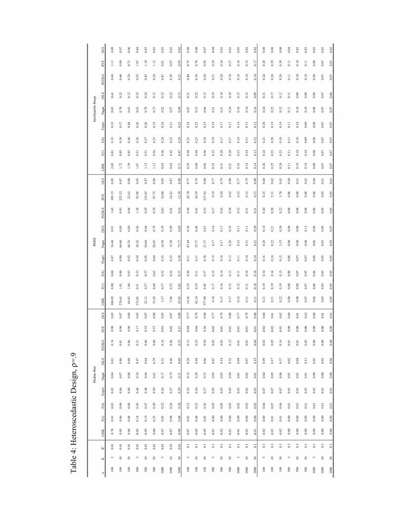
Tabl

e 4:

Het

eros

ceda

stic

Des

ign,

ρ=.

9

Med

ian

Bias

RM

SE

Inte

rQua

rtile

Ran

ge

n K

R2

LIM

L F(

1)

F(4)

F(

opt)

Nag

ar

2SLS

JN

2SLS

JI

VE

OLS

LI

ML

F(1)

F(

4)

F(op

t) N

agar

2S

LS

JN2S

LS

JIV

E O

LS

LIM

L F(

1)

F(4)

F(

opt)

Nag

ar

2SLS

JN

2SLS

JI

VE

OLS

100

5 0.

01

0.78

0.

81

0.83

0.

83

0.84

0.

83

0.74

0.

90

0.85

10

6.05

0.

98

0.88

0.

87

34.4

8 0.

91

1.65

10

5.15

0.

85

2.02

0.

81

0.35

0.

33

0.83

0.

41

0.68

1.

11

0.09

100

10

0.01

0.

85

0.86

0.

86

0.86

0.

87

0.86

0.

81

0.90

0.

87

276.

61

1.01

0.

90

0.90

84

.60

0.89

0.

93

253.

52

0.87

1.

72

0.85

0.

38

0.37

0.

70

0.25

0.

44

0.89

0.

07

100

30

0.01

0.

88

0.88

0.

88

0.88

0.

88

0.88

0.

86

0.90

0.

88

64.8

3 1.

04

0.93

0.

92

44.7

6 0.

89

0.88

22

.63

0.88

1.

39

0.85

0.

46

0.44

0.

63

0.12

0.

24

0.71

0.

06

500

5 0.

01

-0.0

5 0.

18

0.45

0.

46

0.34

0.

47

0.31

0.

17

0.85

37

2.81

0.

51

0.53

0.

54

38.4

2 0.

56

1.28

92

.98

0.85

1.

07

0.51

0.

26

0.26

0.

63

0.35

0.

55

1.07

0.

04

500

10

0.01

-0

.05

0.19

0.

47

0.48

0.

44

0.64

0.

46

0.35

0.

87

22.1

1 0.

57

0.57

0.

58

54.6

4 0.

66

0.59

13

2.65

0.

87

1.15

0.

51

0.27

0.

26

0.70

0.

24

0.43

1.

18

0.03

500

30

0.01

0.

06

0.25

0.

49

0.50

0.

61

0.79

0.

68

0.57

0.

88

33.4

5 0.

68

0.63

0.

64

28.4

3 0.

79

0.70

87

.75

0.88

1.

12

0.56

0.

33

0.32

0.

73

0.13

0.

24

1.13

0.

03

1000

5

0.01

-0

.07

0.03

0.

25

0.26

0.

17

0.31

0.

16

-0.0

3 0.

85

3.17

0.

37

0.32

0.

33

18.5

4 0.

39

0.63

10

.00

0.85

0.

65

0.46

0.

24

0.24

0.

52

0.33

0.

47

0.81

0.

03

1000

10

0.

01

-0.0

7 0.

04

0.26

0.

27

0.19

0.

46

0.26

0.

02

0.87

3.

96

0.35

0.

32

0.33

15

.38

0.49

0.

41

16.4

2 0.

87

0.62

0.

43

0.22

0.

21

0.57

0.

22

0.38

0.

87

0.02

1000

30

0.

01

-0.0

8 0.

04

0.28

0.

29

0.31

0.

69

0.52

0.

21

0.88

53

.85

0.42

0.

37

0.38

73

.77

0.69

0.

54

12.3

0 0.

88

0.71

0.

47

0.24

0.

23

0.69

0.

13

0.23

0.

95

0.02

100

5 0.

1 -0

.07

0.03

0.

23

0.24

0.

15

0.28

0.

13

-0.0

4 0.

77

14.3

6 0.

35

0.30

0.

31

47.4

4 0.

36

0.49

26

.74

0.77

0.

59

0.44

0.

25

0.24

0.

47

0.31

0.

44

0.75

0.

09

100

10

0.1

-0.0

5 0.

04

0.25

0.

26

0.20

0.

44

0.25

0.

04

0.79

42

.14

0.35

0.

31

0.31

35

.77

0.46

0.

41

20.3

9 0.

79

0.60

0.

44

0.23

0.

22

0.53

0.

22

0.38

0.

78

0.08

100

30

0.1

-0.0

5 0.

05

0.26

0.

27

0.33

0.

66

0.50

0.

26

0.80

57

7.96

0.

45

0.37

0.

38

21.3

7 0.

67

0.53

23

7.42

0.

80

0.66

0.

46

0.24

0.

23

0.66

0.

13

0.24

0.

92

0.07

500

5 0.

1 -0

.01

0.00

0.

05

0.05

0.

03

0.07

0.

02

-0.0

2 0.

77

0.18

0.

17

0.15

0.

15

0.17

0.

16

0.17

0.

19

0.77

0.

23

0.22

0.

19

0.19

0.

21

0.19

0.

21

0.24

0.

04

500

10

0.1

-0.0

2 0.

00

0.05

0.

05

0.03

0.

14

0.03

-0

.01

0.79

0.

17

0.16

0.

14

0.14

0.

17

0.17

0.

16

0.20

0.

79

0.21

0.

20

0.17

0.

17

0.21

0.

16

0.20

0.

24

0.03

500

30

0.1

-0.0

1 0.

00

0.05

0.

05

0.04

0.

32

0.12

-0

.01

0.80

0.

17

0.15

0.

13

0.13

0.

26

0.33

0.

18

0.62

0.

80

0.21

0.

20

0.17

0.

17

0.24

0.

10

0.18

0.

27

0.03

1000

5

0.1

-0.0

1 0.

00

0.02

0.

03

0.01

0.

04

0.01

-0

.01

0.77

0.

12

0.12

0.

11

0.11

0.

12

0.11

0.

12

0.12

0.

77

0.16

0.

15

0.14

0.

14

0.16

0.

15

0.16

0.

16

0.03

1000

10

0.

1 -0

.01

0.00

0.

03

0.03

0.

02

0.07

0.

01

-0.0

1 0.

79

0.11

0.

11

0.10

0.

10

0.11

0.

11

0.11

0.

12

0.79

0.

14

0.14

0.

13

0.13

0.

14

0.12

0.

14

0.15

0.

02

1000

30

0.

1 -0

.01

0.00

0.

02

0.03

0.

01

0.19

0.

04

-0.0

1 0.

80

0.11

0.

10

0.10

0.

10

0.12

0.

20

0.11

0.

13

0.80

0.

14

0.13

0.

12

0.12

0.

16

0.09

0.

14

0.17

0.

02

100

5 0.

3 -0

.02

0.00

0.

06

0.07

0.

04

0.09

0.

03

-0.0

2 0.

60

0.21

0.

19

0.16

0.

16

0.20

0.

18

0.20

0.

25

0.60

0.

26

0.24

0.

21

0.20

0.

24

0.21

0.

24

0.28

0.

08

100

10

0.3

-0.0

1 0.

01

0.07

0.

07

0.05

0.

17

0.05

-0

.02

0.61

0.

21

0.19

0.

16

0.16

0.

22

0.21

0.

20

5.31

0.

62

0.25

0.

23

0.20

0.

19

0.25

0.

17

0.24

0.

29

0.08

100

30

0.3

-0.0

2 0.

01

0.06

0.

07

0.06

0.

37

0.16

-0

.01

0.62

0.

22

0.19

0.

15

0.15

3.

15

0.38

0.

22

1.78

0.

63

0.24

0.

23

0.19

0.

19

0.32

0.

12

0.20

0.

39

0.08

500

5 0.

3 0.

00

0.00

0.

01

0.01

0.

01

0.02

0.

01

0.00

0.

60

0.08

0.

08

0.08

0.

08

0.08

0.

08

0.08

0.

08

0.60

0.

11

0.11

0.

11

0.11

0.

11

0.11

0.

11

0.11

0.

04

500

10

0.3

0.00

0.

00

0.01

0.

01

0.01

0.

04

0.01

0.

00

0.61

0.

08

0.08

0.

07

0.07

0.

08

0.08

0.

08

0.08

0.

61

0.10

0.

10

0.10

0.

10

0.10

0.

09

0.10

0.

10

0.03

500

30

0.3

0.00

0.

00

0.01

0.

01

0.01

0.

11

0.02

0.

00

0.62

0.

07

0.07

0.

07

0.07

0.

08

0.12

0.

08

0.08

0.

63

0.10

0.

10

0.09

0.

09

0.10

0.

08

0.10

0.

11

0.03

1000

5

0.3

0.00

0.

00

0.01

0.

01

0.00

0.

01

0.00

0.

00

0.60

0.

06

0.06

0.

06

0.06

0.

06

0.06

0.

06

0.06

0.

60

0.08

0.

08

0.08

0.

08

0.08

0.

08

0.08

0.

08

0.03

1000

10

0.

3 0.

00

0.00

0.

01

0.01

0.

00

0.02

0.

00

0.00

0.

61

0.05

0.

05

0.05

0.

05

0.05

0.

05

0.05

0.

05

0.61

0.

07

0.07

0.

07

0.07

0.

07

0.07

0.

07

0.07

0.

02

1000

30

0.

3 0.

00

0.00

0.

01

0.01

0.

00

0.06

0.

00

0.00

0.

63

0.05

0.

05

0.05

0.

05

0.05

0.

07

0.05

0.

05

0.63

0.

07

0.07

0.

07

0.07

0.

07

0.06

0.

07

0.07

0.

02

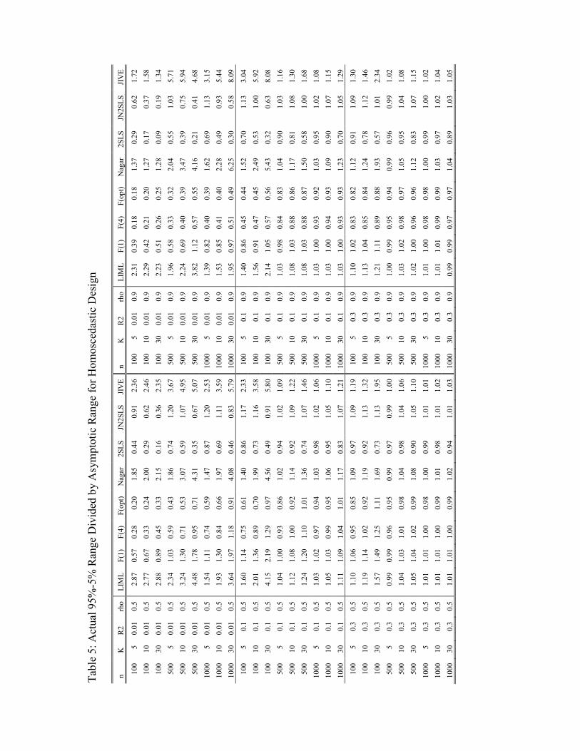
Tabl

e 5:

Act

ual 9

5%-5

% R

ange

Div

ided

by

Asy

mpt

otic

Ran

ge fo

r Hom

osce

dast

ic D

esig

n n

K

R2

rho

LIM

L F(

1)

F(4)

F(

opt)

Nag

ar

2SLS

JN

2SLS

JI

VE

n K

R

2 rh

o LI

ML

F(1)

F(

4)

F(op

t) N

agar

2S

LS

JN2S

LS

JIV

E

100

5 0.

01

0.5

2.87

0.

57

0.28

0.

20

1.85

0.

44

0.91

2.

36

100

5 0.

01

0.9

2.31

0.

39

0.18

0.

18

1.37

0.

29

0.62

1.

72

100

10

0.01

0.

5 2.

77

0.67

0.

33

0.24

2.

00

0.29

0.

62

2.46

10

0 10

0.

01

0.9

2.29

0.

42

0.21

0.

20

1.27

0.

17

0.37

1.

58

100

30

0.01

0.

5 2.

88

0.89

0.

45

0.33

2.

15

0.16

0.

36

2.35

10

0 30

0.

01

0.9

2.23

0.

51

0.26

0.

25

1.28

0.

09

0.19

1.

34

500

5 0.

01

0.5

2.34

1.

03

0.59

0.

43

1.86

0.

74

1.20

3.

67

500

5 0.

01

0.9

1.96

0.

58

0.33

0.

32

2.04

0.

55

1.03

5.

71

500

10

0.01

0.

5 3.

24

1.30

0.

71

0.53

3.

07

0.59

1.

07

4.95

50

0 10

0.

01

0.9

2.24

0.

69

0.40

0.

39

3.47

0.

39

0.75

5.

94

500

30

0.01

0.

5 4.

48

1.78

0.

95

0.71

4.

31

0.35

0.

67

5.07

50

0 30

0.

01

0.9

3.82

1.

12

0.57

0.

55

4.16

0.

21

0.41

4.

68

1000

5

0.01

0.

5 1.

54

1.11

0.

74

0.59

1.

47

0.87

1.

20

2.53

10

00

5 0.

01

0.9

1.39

0.

82

0.40

0.

39

1.62

0.

69

1.13

3.

15

1000

10

0.

01

0.5

1.93

1.

30

0.84

0.

66

1.97

0.

69

1.11

3.

59

1000

10

0.

01

0.9

1.53

0.

85

0.41

0.

40

2.28

0.

49

0.93

5.

44

1000

30

0.

01

0.5

3.64

1.

97

1.18

0.

91

4.08

0.

46

0.83

5.

79

1000

30

0.

01

0.9

1.95

0.

97

0.51

0.

49

6.25

0.

30

0.58

8.

09

100

5 0.

1 0.

5 1.

60

1.14

0.

75

0.61

1.

40

0.86

1.

17

2.33

10

0 5

0.1

0.9

1.40

0.

86

0.45

0.

44

1.52

0.

70

1.13

3.

04

100

10

0.1

0.5

2.01

1.

36

0.89

0.

70

1.99

0.

73

1.16

3.

58

100

10

0.1

0.9

1.56

0.

91

0.47

0.

45

2.49

0.

53

1.00

5.

92

100

30

0.1

0.5

4.15

2.

19

1.29

0.

97

4.56

0.

49

0.91

5.

80

100

30

0.1

0.9

2.14

1.

05

0.57

0.

56

5.43

0.

32

0.63

8.

08

500

5 0.

1 0.

5 1.

04

1.00

0.

93

0.86

1.

02

0.94

1.

02

1.09

50

0 5

0.1

0.9

1.03

0.

98

0.84

0.

83

1.04

0.

90

1.03

1.

16

500

10

0.1

0.5

1.12

1.

08

1.00

0.

92

1.14

0.

92

1.09

1.

22

500

10

0.1

0.9

1.08

1.

03

0.88

0.

86

1.17

0.

81

1.08

1.

30

500

30

0.1

0.5

1.24

1.

20

1.10

1.

01

1.36

0.

74

1.07

1.

46

500

30

0.1

0.9

1.08

1.

03

0.88

0.

87

1.50

0.

58

1.00

1.

68

1000

5

0.1

0.5

1.03

1.

02

0.97

0.

94

1.03

0.

98

1.02

1.

06

1000

5

0.1

0.9

1.03

1.

00

0.93

0.

92

1.03

0.

95

1.02

1.

08

1000

10

0.

1 0.

5 1.

05

1.03

0.

99

0.95

1.

06

0.95

1.

05

1.10

10

00

10

0.1

0.9

1.03

1.

00

0.94

0.

93

1.09

0.

90

1.07

1.

15

1000

30

0.

1 0.

5 1.

11

1.09

1.

04

1.01

1.

17

0.83

1.

07

1.21

10

00

30

0.1

0.9

1.03

1.

00

0.93

0.

93

1.23

0.

70

1.05

1.

29

100

5 0.

3 0.

5 1.

10

1.06

0.

95

0.85

1.

09

0.97

1.

09

1.19

10

0 5

0.3

0.9

1.10

1.

02

0.83

0.

82

1.12

0.

91

1.09

1.

30

100

10

0.3

0.5

1.19

1.

14

1.02

0.

92

1.19

0.

92

1.13

1.

32

100

10

0.3

0.9

1.13

1.

04

0.85

0.

84

1.24

0.

78

1.12

1.

46

100

30

0.3

0.5

1.57

1.

49

1.25

1.

11

1.69

0.

73

1.13

1.

95

100

30

0.3

0.9

1.21

1.

11

0.89

0.

88

1.93

0.

57

1.01

2.

34

500

5 0.

3 0.

5 0.

99

0.99

0.

96

0.95

0.

99

0.97

0.

99

1.00

50

0 5

0.3

0.9

1.00

0.

99

0.95

0.

94

0.99

0.

96

0.99

1.

02

500

10

0.3

0.5

1.04

1.

03

1.01

0.

98

1.04

0.

98

1.04

1.

06

500

10

0.3

0.9

1.03

1.

02

0.98

0.

97

1.05

0.

95

1.04

1.

08

500

30

0.3

0.5

1.05

1.

04

1.02

0.

99

1.08

0.

90

1.05

1.

10

500

30

0.3

0.9

1.02

1.

00

0.96

0.

96

1.12

0.

83

1.07

1.

15

1000

5

0.3

0.5

1.01

1.

01

1.00

0.

98

1.00

0.

99

1.01

1.

01

1000

5

0.3

0.9

1.01

1.

00

0.98

0.

98

1.00

0.

99

1.00

1.

02

1000

10

0.

3 0.

5 1.

01

1.01

1.

00

0.99

1.

01

0.98

1.

01

1.02

10

00

10

0.3

0.9

1.01

1.

01

0.99

0.

99

1.03

0.

97

1.02

1.

04

1000

30

0.

3 0.

5 1.

01

1.01

1.

00

0.99

1.

02

0.94

1.

01

1.03

10

00

30

0.3

0.9

0.99

0.

99

0.97

0.

97

1.04

0.

89

1.03

1.

05

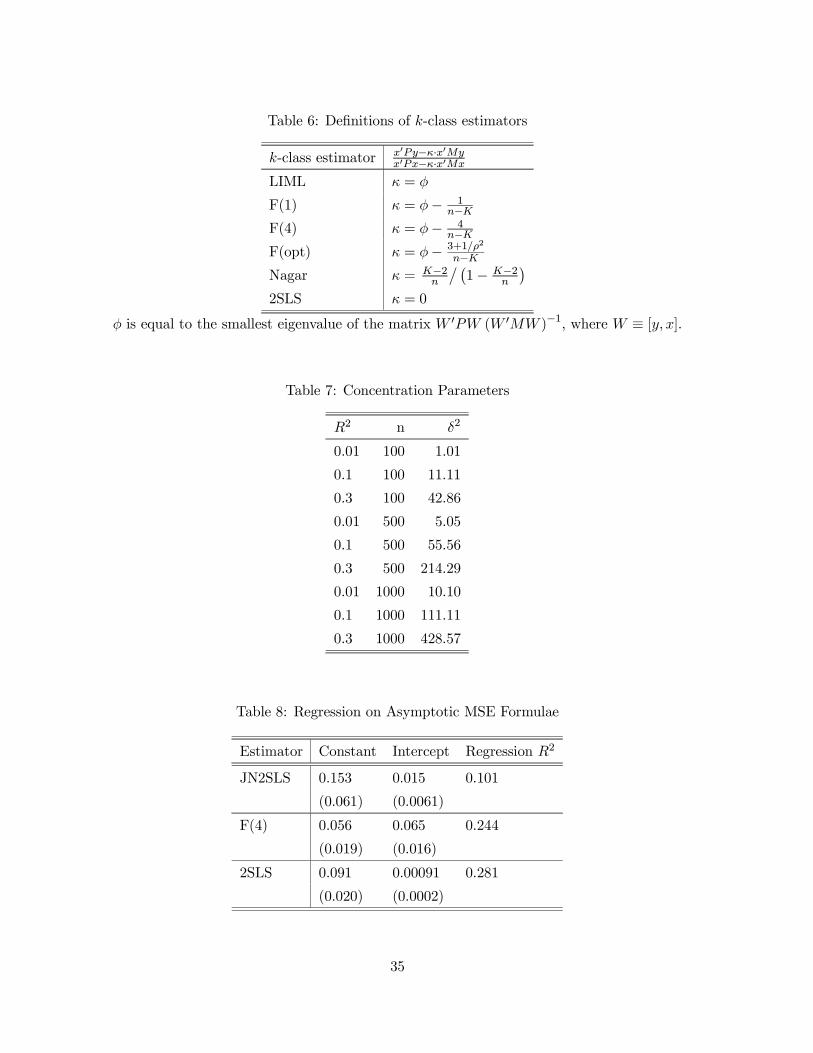
Table 6: DeÞnitions of k-class estimators

k-class estimator x0Py−κ·x0Myx0Px−κ·x0Mx

LIML κ = φ

F(1) κ = φ− 1n−K

F(4) κ = φ− 4n−K

F(opt) κ = φ− 3+1/ρ2

n−KNagar κ = K−2

n

±¡1− K−2

n

¢2SLS κ = 0

φ is equal to the smallest eigenvalue of the matrix W 0PW (W 0MW )−1, where W ≡ [y, x].

Table 7: Concentration Parameters

R2 n δ2

0.01 100 1.01

0.1 100 11.11

0.3 100 42.86

0.01 500 5.05

0.1 500 55.56

0.3 500 214.29

0.01 1000 10.10

0.1 1000 111.11

0.3 1000 428.57

Table 8: Regression on Asymptotic MSE Formulae

Estimator Constant Intercept Regression R2

JN2SLS 0.153 0.015 0.101

(0.061) (0.0061)

F(4) 0.056 0.065 0.244

(0.019) (0.016)

2SLS 0.091 0.00091 0.281

(0.020) (0.0002)

35

Table 9: Regression on Asymptotic MSE Formulae

Estimator C1 C2 Regression R2

JN2SLS 1.74 -.030 .665

(.168) (.006)

F(4) .807 -.173 .957

(.023) (.009)

2SLS .384 .0003 .407

(.064) (.0002)

Table 10: Regression of Log MSE

RHS Variables JN2SLS F(4) 2SLS

logn -.955 -1.01 -.999

(.037) (.025) (.036)

log ρ2 .570 .568 .961

(.108) (.074) (.106)

logK -.060 .098 .389

(.078) (.053) (.077)

logRatio 1.10 .930 .880

(.041) (.028) (.040)

Regression R2 .950 .969 .939

36

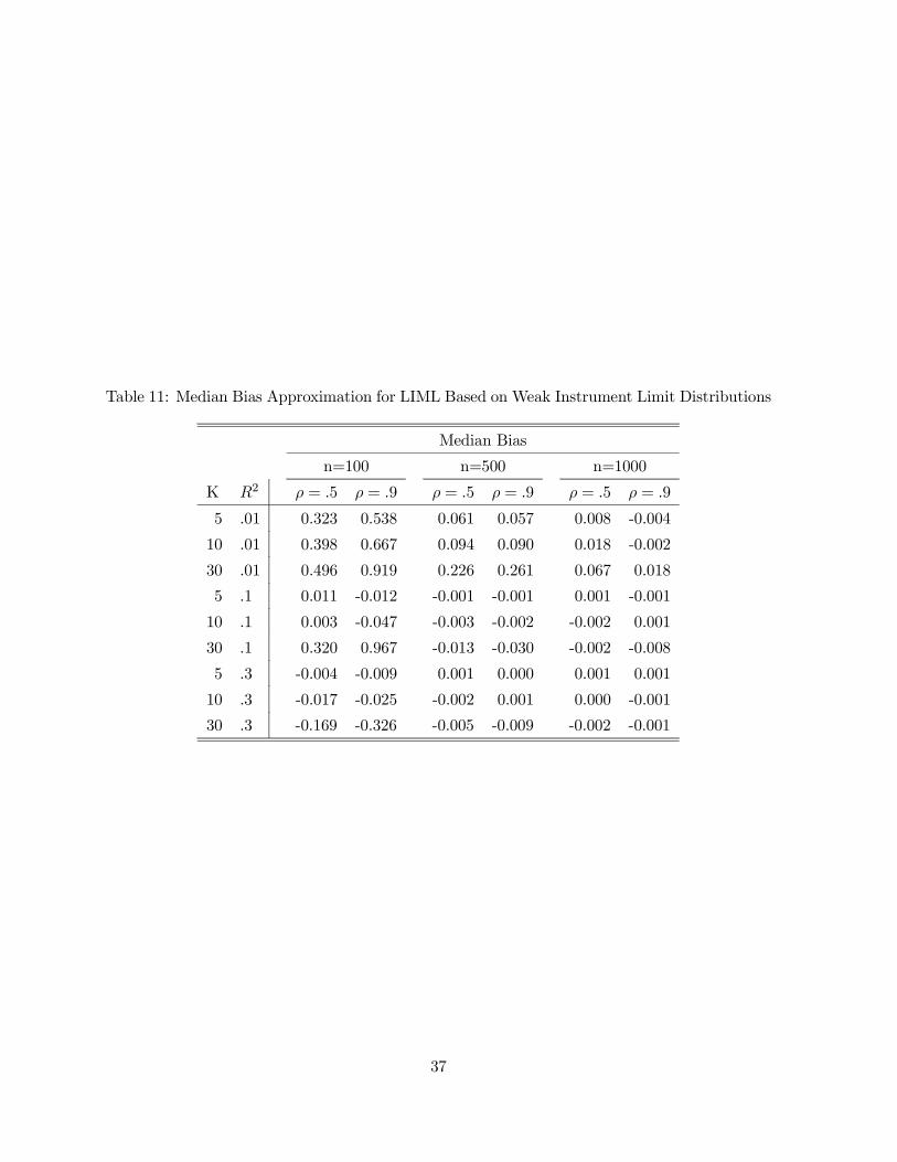
Table 11: Median Bias Approximation for LIML Based on Weak Instrument Limit Distributions

Median Bias

n=100 n=500 n=1000

K R2 ρ = .5 ρ = .9 ρ = .5 ρ = .9 ρ = .5 ρ = .9

5 .01 0.323 0.538 0.061 0.057 0.008 -0.004

10 .01 0.398 0.667 0.094 0.090 0.018 -0.002

30 .01 0.496 0.919 0.226 0.261 0.067 0.018

5 .1 0.011 -0.012 -0.001 -0.001 0.001 -0.001

10 .1 0.003 -0.047 -0.003 -0.002 -0.002 0.001

30 .1 0.320 0.967 -0.013 -0.030 -0.002 -0.008

5 .3 -0.004 -0.009 0.001 0.000 0.001 0.001

10 .3 -0.017 -0.025 -0.002 0.001 0.000 -0.001

30 .3 -0.169 -0.326 -0.005 -0.009 -0.002 -0.001

37

estimation with weak instruments: accuracy of higher order...

Documents