the zero lower bound and estimation accuracy
TRANSCRIPT
Working Paper 1804 Research Department https://doi.org/10.24149/wp1804r1
Working papers from the Federal Reserve Bank of Dallas are preliminary drafts circulated for professional comment. The views in this paper are those of the authors and do not necessarily reflect the views of the Federal Reserve Bank of Dallas or the Federal Reserve System. Any errors or omissions are the responsibility of the authors.
The Zero Lower Bound and Estimation Accuracy
Tyler Atkinson, Alexander W. Richter and Nathaniel A. Throckmorton

The Zero Lower Bound and Estimation Accuracy*
Tyler Atkinson†, Alexander W. Richter‡, and Nathaniel A. Throckmorton§
First Draft: May 7, 2018
This Draft: February 1, 2019
Abstract
During the Great Recession, many central banks lowered their policy rate to its zero lower bound (ZLB), creating a kink in the policy rule and calling into question linear estimation methods. There are two promising alternatives: estimate a fully nonlinear model that accounts for precautionary savings effects of the ZLB or a piecewise linear model that is much faster but ignores the precautionary savings effects. Repeated estimation with artificial datasets reveals some advantages of the nonlinear model, but they are not large enough to justify the longer estimation time, regardless of the ZLB duration in the data. Misspecification of the estimated models has a much larger impact on accuracy. It biases the parameter estimates and creates significant differences between the predictions of the models and the data generating process.
Keywords: Bayesian Estimation; Projection Methods; Particle Filter; OccBin; Inversion Filter
JEL Classifications: C11; C32; C51; E43
*We thank Boragan Aruoba, Alex Chudik, Marc Giannoni, Matthias Hartmann, Rob Hicks, Ben Johannsen, Giorgio Primiceri, Sanjay Singh, Kei-Mu Yi, and an anonymous referee for useful suggestions that improved the paper. We also thank Chris Stackpole and Eric Walter for supporting the supercomputers at our institutions. A previous version of this paper circulated with the title: “The Accuracy of Linear and Nonlinear Estimation in the Presence of the Zero Lower Bound.” This research was completed with supercomputing resources provided by the Federal Reserve Bank of Kansas City, William & Mary, Auburn University, the University of Texas at Dallas, the Texas Advanced Computing Center, and Southern Methodist University. The views expressed in this paper are those of the authors and do not necessarily reflect the views of the Federal Reserve Bank of Dallas or the Federal Reserve System.†Tyler Atkinson, Research Department, Federal Reserve Bank of Dallas, 2200 N. Pearl Street, Dallas, TX 75201,
[email protected]. ‡Alexander W. Richter, Research Department, Federal Reserve Bank of Dallas, 2200 N. Pearl Street, Dallas, TX 75201,
[email protected]. §Nathaniel A. Throckmorton, Department of Economics, William & Mary, P.O. Box 8795, Williamsburg, VA 23187,[email protected].
ATKINSON, RICHTER & T HROCKMORTON: THE ZERO LOWER BOUND AND ESTIMATION ACCURACY
1 INTRODUCTION
Using Bayesian methods to estimate linear dynamic stochastic general equilibrium (DSGE) models
has become common practice in the literature over the last 20years. Many central banks also use
these models for forecasting and counterfactual simulations. The estimation procedure sequentially
draws parameters from a proposal distribution, solves the model given that draw, and then evalu-
ates the likelihood function. With linearity and normally distributed shocks, the model solves in a
fraction of a second and it is easy to exactly evaluate the likelihood function with a Kalman filter.1
The financial crisis and subsequent recession compelled many central banks to take unprece-
dented action to reduce their policy rate to its zero lower bound (ZLB), calling into question linear
estimation methods. The ZLB constraint presents a challenge for empirical work because it creates
a kink in the central bank’s policy rule. The constraint has always existed, but when policy rates
were well above zero and the likelihood of hitting the constraint was negligible, it was reasonable
to ignore it. The lengthy period of near zero policy rates over the last decade and the increased like-
lihood of future ZLB events due to estimates of a lower natural rate has forced researchers to think
more carefully about the ZLB constraint and its implications (e.g., Laubach and Williams, 2016).
There are two promising estimation methods used in the literature that account for the ZLB
constraint in DSGE models. The first method estimates a fullynonlinear model with an occasion-
ally binding ZLB constraint (e.g., Gust et al., 2017; Planteet al., 2018; Richter and Throckmorton,
2016). This method provides the most comprehensive treatment of the ZLB constraint but is nu-
merically intensive. It uses projection methods to solve the nonlinear model and a particle filter to
evaluate the likelihood function for each draw from the posterior distribution (henceforth, NL-PF).2
The second method estimates a piecewise linear version of the nonlinear model (e.g., Guerri-
eri and Iacoviello, 2017). The model is solved using the OccBin toolbox developed by Guerrieri
and Iacoviello (2015). The likelihood is evaluated using aninversion filter, which solves for the
shocks that minimize the distance between the data and the model predictions each period. The
benefit of this method (henceforth, PW-IF) is that it is nearly as fast as estimating a linear model
with a Kalman filter while still capturing the kink in the decision rules created by the ZLB con-
straint. However, PW-IF differs from NL-PF in two ways. One,households do not account for the
possibility that the ZLB may bind in the future if it does not bind in the current period, which is in-
consistent with survey data. Two, the inversion filter removes the interest rate as an observable and
sets the monetary policy shock to zero when the ZLB binds, whereas the particle filter estimates
those shocks given the data. The question is whether PW-IF isan adequate substitute for NL-PF.
1Schorfheide (2000) and Otrok (2001) were the first to use these methods to generate draws from the posteriordistribution of a linear DSGE model. See An and Schorfheide (2007) and Herbst and Schorfheide (2016) for examples.
2Several papers examine the effects of the ZLB constraint in acalibratednonlinear model using projection methodssimilar to ours (e.g., Aruoba et al., 2018; Fernandez-Villaverde et al., 2015; Gavin et al., 2015; Keen et al., 2017;Mertens and Ravn, 2014; Nakata, 2017; Nakov, 2008; Ngo, 2014; Richter and Throckmorton, 2015; Wolman, 2005).
1
ATKINSON, RICHTER & T HROCKMORTON: THE ZERO LOWER BOUND AND ESTIMATION ACCURACY
This paper compares the accuracy of the two estimation methods. We specify a true parameter-
ization of a medium-scale nonlinear model with an occasionally binding ZLB constraint, solve the
model with a projection method, and generate a large sample of datasets. The datasets either con-
tain no ZLB events or a single event with various durations tounderstand the influence of the ZLB
on the posterior estimates. For each dataset, we use NL-PF and PW-IF to estimate a small-scale,
but nested, version of the medium-scale model that generates the data. We also estimate the linear
model with a Kalman filter (henceforth, Lin-KF), since it wasthe most common method before the
Great Recession. The small-scale model excludes features of the medium-scale model that others
have shown are empirically important. The difference between the two models—referred to as
misspecification—account for the practical reality that all models are misspecified. It also sheds
light on the merits of estimating a simpler, more misspecified, model with NL-PF, versus a richer,
less misspecified, model with PW-IF that is numerically too costly with fully nonlinear methods.
We measure accuracy by comparing the parameter estimates, predictions of the notional interest
rate, expected frequency and duration of the ZLB, simulatedresponses to a severe recession, and
forecasting performance. While our posterior estimates reveal some advantages of NL-PF, they
are not large enough to justify the significantly longer estimation time, regardless of the ZLB
duration in the data. This key finding holds because the precautionary savings effects of the ZLB
and the effects of other nonlinearities, independent of theZLB, are small in canonical models.
Model misspecification has a larger impact. It biases the parameter estimates and creates significant
differences between the predictions of the two estimated models and the data generating process.
Since there is not a large advantage to estimating the fully nonlinear model over an equally
misspecified piecewise linear model, our results indicate that researchers are better off reducing
misspecification by estimating a richer piecewise linear model than a simpler but computationally
feasible nonlinear model when the ZLB binds in the data. Thisimportant finding opens the door
to promising new research on the implications of the ZLB constraint. The results also provide a
useful benchmark for future research that explores other nonlinear features or estimation methods.
Our paper is the first to compare different estimation methods that account for the ZLB con-
straint. Others compare nonlinear estimation methods to linear methods. Fernandez-Villaverde
and Rubio-Ramırez (2005) show that a neoclassical growth model estimated with NL-PF predicts
moments closer to the true moments than the estimates from Lin-KF using two artificial datasets
and actual data. The primary source of nonlinearity in theirmodel is high risk aversion. Hirose and
Inoue (2016) generate artificial datasets from a linear model where the ZLB constraint is imposed
using anticipated monetary policy shocks and then apply Lin-KF to estimate the model without
the constraint. They find the estimated parameters, impulseresponses, and structural shocks be-
come less accurate as the frequency and duration of ZLB events increase in the data. Hirose and
Sunakawa (2015) extend that work by generating data from a nonlinear model and reexamine the
2
ATKINSON, RICHTER & T HROCKMORTON: THE ZERO LOWER BOUND AND ESTIMATION ACCURACY
bias. None of these papers introduce misspecification, which is an important aspect of our analysis.
We also build on recent empirical work that analyzes the implications of the ZLB constraint
(e.g., Gust et al., 2017; Iiboshi et al., 2018; Plante et al.,2018; Richter and Throckmorton, 2016).
These papers use NL-PF to estimate a nonlinear model similarto ours using actual data from the
U.S. or Japan that includes the ZLB period. Our contributionis to examine the accuracy of these
nonlinear estimation methods and show under what conditions they outperform other approaches.
The measurement error (ME) in the observation equation of the filter is a key aspect of the
estimation procedure that could potentially affect the accuracy of the parameter estimates. Unlike
the inversion filter, the particle filter requires positive ME variances to prevent degeneracy—a
situation when the likelihood is inaccurate. The literature has used a wide range of different values,
with limited investigation on how they impact accuracy. Canova et al. (2014) show the downside
of introducing ME is that the posterior distributions of some parameters do not contain the truth
in a DSGE model estimated with Lin-KF. Cuba-Borda et al. (2017) show that ME in the particle
filter reduces the accuracy of the likelihood function usinga calibrated model with an occasionally
binding borrowing constraint. Our analysis provides a potentially important role for ME because
it includes model misspecification. We find larger ME variances improve the accuracy of some
parameters, but the benefits are more than offset by decreases in the accuracy of other parameters.3
The paper proceeds as follows.Section 2describes our data generating process and artificial
datasets.Section 3outlines the estimated model and numerical methods.Section 4shows our pos-
terior estimates and several measures of accuracy for each estimation method.Section 5concludes.
2 DATA GENERATING PROCESS
To test the accuracy of recent estimation methods, we generate a large number of artificial datasets
from a canonical New Keynesian model with capital and an occasionally binding ZLB constraint.
2.1 FIRMS The production sector consists of a continuum of monopolistically competitive inter-
mediate goods firms and a final goods firm. Intermediate firmf ∈ [0, 1] produces a differentiated
good,y(f), according toyt(f) = (υtkt−1(f))α(ztnt(f))
1−α, wheren(f) is the labor hired by firm
f andk(f) is the capital rented by firmf . zt = gtzt−1 is technology andυ is the capital utilization
rate, which are both common across firms. Deviations from thesteady-state growth rate,g, follow
gt = g + σgεg,t, εg ∼ N(0, 1). (1)
The final goods firm purchases output from each intermediate firm to produce the final good,
yt ≡ [∫ 1
0yt(f)
(θp−1)/θpdf ]θp/(θp−1), whereθp > 1 is the elasticity of substitution. Dividend max-
3Herbst and Schorfheide (2018) develop a tempered particle filter that sequentially reduces the ME variances. Theyassess accuracy against the Kalman filter on U.S. data with a linear model and find it outperforms the untempered filter.
3

ATKINSON, RICHTER & T HROCKMORTON: THE ZERO LOWER BOUND AND ESTIMATION ACCURACY
imization determines the demand for intermediate goodf , yt(f) = (pt(f)/pt)−θpyt, wherept =
[∫ 1
0pt(f)
1−θpdf ]1/(1−θp) is the price level. Following Rotemberg (1982), intermediate firms pay a
price adjustment cost,adjpt (f) ≡ ϕp(pt(f)/(πpt−1(f))−1)2yt/2, whereϕp > 0 scales the cost and
π is the steady-state gross inflation rate. Given this cost, firm f choosesnt(f), kt−1(f), andpt(f)
to maximize the expected discounted present value of futuredividends,Et
∑
∞
k=t qt,kdk(f), subject
to its production function and the demand for its product, whereqt,t ≡ 1, qt,t+1 ≡ β(λt/λt+1) is
the pricing kernel between periodst andt+ 1, qt,k ≡∏k>t
j=t+1 qj−1,j, anddt(f) = pt(f)yt(f)/pt −
wtnt(f)− rkt υtkt−1(f)− adjpt (f). In symmetric equilibrium, the optimality conditions reduce to
yt = (υtkt−1)α(ztnt)
1−α, (2)
wt = (1− α)mctyt/nt, (3)
rkt = αmctyt/(υtkt−1), (4)
ϕp(πt/π − 1)(πt/π) = 1− θp + θpmct + βϕpEt[(λt/λt+1)(πt+1/π − 1)(πt+1/π)yt+1/yt], (5)
whereπt = pt/pt−1 is the gross inflation rate. Ifϕp = 0, the real marginal cost of producing a unit
of output (mct) equals(θp − 1)/θp, which is the inverse of the markup of price over marginal cost.
2.2 HOUSEHOLDS Each household consists of a unit mass of members who supply differen-
tiated types of labor,n(ℓ), at real wage ratew(ℓ). A perfectly competitive labor union bundles
the labor types to produce an aggregate labor product,nt ≡ [∫ 1
0nt(ℓ)
(θw−1)/θwdℓ]θw/(θw−1), where
θw > 1 is the elasticity of substitution. Dividend maximization determines the demand for labor
typeℓ, nt(ℓ) = (wt(ℓ)/wt)−θwnt, wherewt = [
∫ 1
0wt(ℓ)
1−θwdℓ]1/(1−θw) is the aggregate real wage.
The households choose{ct, nt, bt, xt, kt, υt}∞
t=0 to maximize expected lifetime utility given by
E0
∑
∞
t=0 βt[log(ct − hcat−1) − χ
∫ 1
0nt(ℓ)
1+ηdℓ/(1 + η)], whereβ is the discount factor,χ deter-
mines steady-state labor,1/η is the Frisch labor supply elasticity,c is consumption,ca is aggregate
consumption,h is the degree of external habit persistence,b is the real value of a privately-issued1-
period nominal bond,x is investment, andE0 is an expectation operator conditional on information
available in period0. Following Chugh (2006), the nominal wage rate for each labor type is sub-
ject to an adjustment cost,adjwt (ℓ) = ϕw(wgt (ℓ)− 1)2yt/2, wherewg
t (ℓ) = πtwt(ℓ)/(πgwt−1(ℓ)) is
nominal wage growth relative its steady-state. The cost of utilizing the capital shock,u, is given by
ut = rk(exp(συ(υt − 1))− 1)/συ, (6)
whereσυ ≥ 0 scales the cost. Given the two costs, the household’s budgetconstraint is given by
ct + xt + bt/(stit) + utkt−1 +∫ 1
0adjwt (ℓ)dℓ =
∫ 1
0wt(ℓ)nt(ℓ)dℓ+ rkt υtkt−1 + bt−1/πt + dt,
wherei is the gross nominal interest rate,rk is the capital rental rate, andd is a real dividend from
4
ATKINSON, RICHTER & T HROCKMORTON: THE ZERO LOWER BOUND AND ESTIMATION ACCURACY
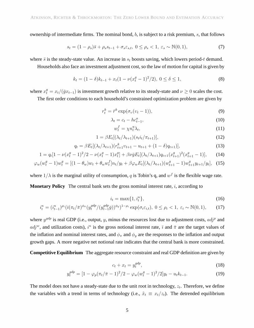
ownership of intermediate firms. The nominal bond,b, is subject to a risk premium,s, that follows
st = (1− ρs)s+ ρsst−1 + σsεs,t, 0 ≤ ρs < 1, εs ∼ N(0, 1), (7)
wheres is the steady-state value. An increase inst boosts saving, which lowers period-t demand.
Households also face an investment adjustment cost, so the law of motion for capital is given by
kt = (1− δ)kt−1 + xt(1− ν(xgt − 1)2/2), 0 ≤ δ ≤ 1, (8)
wherexgt = xt/(gxt−1) is investment growth relative to its steady-state andν ≥ 0 scales the cost.
The first order conditions to each household’s constrained optimization problem are given by
rkt = rk exp(συ(υt − 1)), (9)
λt = ct − hcat−1, (10)
wft = χnη
tλt, (11)
1 = βEt[(λt/λt+1)(stit/πt+1)], (12)
qt = βEt[(λt/λt+1)(rkt+1υt+1 − ut+1 + (1− δ)qt+1)], (13)
1 = qt[1− ν(xgt − 1)2/2− ν(xg
t − 1)xgt ] + βνgEt[(λt/λt+1)qt+1(x
gt+1)
2(xgt+1 − 1)], (14)
ϕw(wgt − 1)wg
t = [(1− θw)wt + θwwft ]nt/yt + βϕwEt[(λt/λt+1)(w
gt+1 − 1)wg
t+1yt+1/yt], (15)
where1/λ is the marginal utility of consumption,q is Tobin’s q, andwf is the flexible wage rate.
Monetary Policy The central bank sets the gross nominal interest rate,i, according to
it = max{1, int }, (16)
int = (int−1)ρi (ı(πt/π)
φπ(ygdpt /(ygdpt−1g))φy)1−ρi exp(σiεi,t), 0 ≤ ρi < 1, εi ∼ N(0, 1), (17)
whereygdp is real GDP (i.e., output,y, minus the resources lost due to adjustment costs,adjp and
adjw, and utilization costs),in is the gross notional interest rate,ı and π are the target values of
the inflation and nominal interest rates, andφπ andφy are the responses to the inflation and output
growth gaps. A more negative net notional rate indicates that the central bank is more constrained.
Competitive Equilibrium The aggregate resource constraint and real GDP definition are given by
ct + xt = ygdpt , (18)
ygdpt = [1− ϕp(πt/π − 1)2/2− ϕw(wgt − 1)2/2]yt − utkt−1. (19)
The model does not have a steady-state due to the unit root in technology,zt. Therefore, we define
the variables with a trend in terms of technology (i.e.,xt ≡ xt/zt). The detrended equilibrium
5

ATKINSON, RICHTER & T HROCKMORTON: THE ZERO LOWER BOUND AND ESTIMATION ACCURACY
system is provided inAppendix A. A competitive equilibrium consists of sequences of quan-
tities,{ct, yt, ygdpt , xg
t , ygt , nt, kt, xt}
∞
t=0, prices,{wt, wft , w
gt , it, i
nt , πt, λt, υt, ut, qt, r
kt , mct}
∞
t=0, and
exogenous variables,{st, gt}∞t=0, that satisfy the detrended equilibrium system, given the initial
conditions,{c−1, in−1, k−1, x−1, w−1, s0, g0, εi,0}, and three sequences of shocks,{εg,t, εs,t, εi,t}
∞
t=1.
Subjective Discount Factor β 0.9949 Rotemberg Price Adjustment Cost ϕp 100Frisch Labor Supply Elasticity 1/η 3 Rotemberg Wage Adjustment Cost ϕw 100Price Elasticity of Substitution θp 6 Capital Utilization Curvature συ 5Wage Elasticity of Substitution θw 6 Inflation Gap Response φπ 2Steady-State Labor Hours n 0.3333 Output Growth Gap Response φy 0.5Steady-State Risk Premium s 1.0058 Habit Persistence h 0.8Steady-State Growth Rate g 1.0034 Risk Premium Persistence ρs 0.8Steady-State Inflation Rate π 1.0053 Notional Rate Persistence ρi 0.8Capital Share of Income α 0.35 Technology Growth Shock SD σg 0.005Capital Depreciation Rate δ 0.025 Risk Premium Shock SD σs 0.005Investment Adjustment Cost ν 4 Notional Interest Rate Shock SD σi 0.002
Table 1: Parameter values for the data generating process.
2.3 PARAMETER VALUES Table 1shows the true model parameters. The parameters were cho-
sen so our data generating process is characteristic of U.S.data. The steady-state growth rate (g),
inflation rate (π), risk-premium (s), and capital share of income (α) are equal to the time aver-
ages of per capita real GDP growth, the percent change in the GDP implicit price deflator, the
Baa corporate bond yield relative to the yield on the 10-YearTreasury, and the Fernald (2012)
utilization-adjusted quarterly-TFP estimates of the capital share of income from 1988Q1-2017Q4.
The subjective discount factor,β, is set to0.9949, which is the time average of the values im-
plied by the steady-state consumption Euler equation and the federal funds rate. The corresponding
annualized steady-state nominal interest rate is3.3%, which is consistent with the sample average
and current long-run estimates of the federal funds rate. The leisure preference parameter,χ, is set
so steady-state labor equals1/3 of the available time. The elasticities of substitution between inter-
mediate goods and labor types,θp andθw, are set to6, which correspond to a20% average markup
in each sector and match the values used in Gust et al. (2017).The Frisch elasticity of labor supply,
1/η, is set to3 to match the macro estimate in Peterman (2016). The remaining parameters are set
to round numbers that are in line with the posterior estimates from similar models in the literature.
2.4 SOLUTION AND SIMULATION METHODS We solve the nonlinear model with the policy
function iteration algorithm described in Richter et al. (2014), which is based on the theoretical
work on monotone operators in Coleman (1991). We discretizethe endogenous state variables and
approximate the exogenous states,st, gt, andεi,t using theN-state Markov chain in Rouwenhorst
(1995). The Rouwenhorst method is attractive because it only requires us to interpolate along the
dimensions of the endogenous state variables, which makes the solution more accurate and faster
6
ATKINSON, RICHTER & T HROCKMORTON: THE ZERO LOWER BOUND AND ESTIMATION ACCURACY
than quadrature methods. To obtain initial conjectures forthe nonlinear policy functions, we solve
the level-linear analogue of our nonlinear model with Sims’s (2002) gensys algorithm. Then we
minimize the Euler equation errors on every node in the statespace and compute the maximum
distance between the updated policy functions and the initial conjectures. Finally, we replace the
initial conjectures with the updated policy functions and iterate until the maximum distance is
below the tolerance level. SeeAppendix Bfor a more detailed description of the solution method.
We generate data for output growth, the inflation rate, and the nominal interest rate by simulat-
ing the model using the nonlinear policy functions, so the observables are given byxt = [ygt , πt, it].
Each simulation is initialized with a draw from the ergodic distribution and contains120 quarters,
which is similar to what is typically used when estimating models with actual data. We use samples
from the data generating process that either have no ZLB events or a singular ZLB event that makes
up5%, 10%, 15%, 20%, and25% of the sample. Since our sample is120 quarters, the ZLB events
are either6, 12, 18, 24, or30 quarters long. The longest ZLB events reflect the experiences of some
advanced economies, such as the U.S. since the Great Recession or Japan. We create50 datasets
for each ZLB duration and then report measures of accuracy based on the posterior mean estimates.
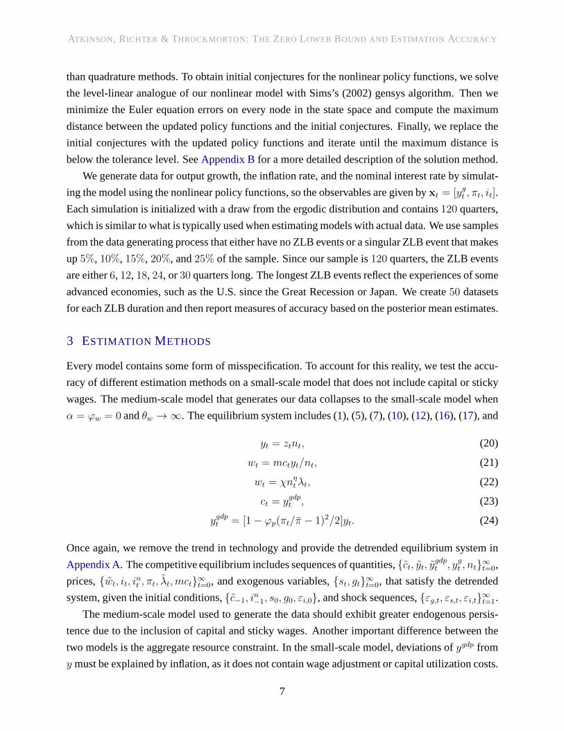
3 ESTIMATION METHODS
Every model contains some form of misspecification. To account for this reality, we test the accu-
racy of different estimation methods on a small-scale modelthat does not include capital or sticky
wages. The medium-scale model that generates our data collapses to the small-scale model when
α = ϕw = 0 andθw → ∞. The equilibrium system includes (1), (5), (7), (10), (12), (16), (17), and
yt = ztnt, (20)
wt = mctyt/nt, (21)
wt = χnηtλt, (22)
ct = ygdpt , (23)
ygdpt = [1− ϕp(πt/π − 1)2/2]yt. (24)
Once again, we remove the trend in technology and provide thedetrended equilibrium system in
Appendix A. The competitive equilibrium includes sequences of quantities,{ct, yt, ygdpt , ygt , nt}
∞
t=0,
prices,{wt, it, int , πt, λt, mct}
∞
t=0, and exogenous variables,{st, gt}∞t=0, that satisfy the detrended
system, given the initial conditions,{c−1, in−1, s0, g0, εi,0}, and shock sequences,{εg,t, εs,t, εi,t}
∞
t=1.
The medium-scale model used to generate the data should exhibit greater endogenous persis-
tence due to the inclusion of capital and sticky wages. Another important difference between the
two models is the aggregate resource constraint. In the small-scale model, deviations ofygdp from
y must be explained by inflation, as it does not contain wage adjustment or capital utilization costs.
7

ATKINSON, RICHTER & T HROCKMORTON: THE ZERO LOWER BOUND AND ESTIMATION ACCURACY
We estimate the small-scale model with Bayesian methods. For each dataset, we draw param-
eters from a proposal distribution, solve the model conditional on the draw, and filter the data to
evaluate the likelihood function within a random walk Metropolis-Hastings algorithm. Within this
framework, we test the accuracy of two promising estimationmethods that account for the ZLB.
The first method estimates the fully nonlinear model with a particle filter (NL-PF). We solve
the model with the same algorithm we used to generate our datasets. To filter the data, we follow
Algorithm 14 in Herbst and Schorfheide (2016) and adapt the basic bootstrap particle filter de-
scribed in Fernandez-Villaverde and Rubio-Ramırez (2007) to include the information contained
in the current observation, so the model better matches extreme outliers in the data. NL-PF is well-
equipped to handle the nonlinearities in the data, but it is also the most computationally intensive.
NL-PF requires solving the fully nonlinear model and performing a large number of simulations to
evaluate the likelihood function for each draw in the randomwalk Metropolis-Hastings algorithm.
Appendix Cprovides a more detailed description of the estimation algorithm and the particle filter.
The second method estimates a piecewise linear version of the nonlinear model with an inver-
sion filter. To solve the model, we use the OccBin toolbox developed by Guerrieri and Iacoviello
(2015). The algorithm separates the model into two regimes.In one regime, the ZLB constraint
is slack, and the decision rules from the unconstrained linear model are used. In the other regime,
the ZLB binds and backwards induction within a guess and verify method solves for the decision
rules. For example, if the ZLB binds in the current period, aninitial conjecture is made for how
many quarters the nominal interest rate will remain at the ZLB. Starting far enough in the future,
the algorithm uses the decision rules for when the ZLB does not bind and iterates backward to the
current period. The algorithm switches to the decision rules for the ZLB regime when the simu-
lated nominal interest rate indicates that the ZLB binds. The simulation implies a new guess for
the ZLB duration. The algorithm iterates until the implied ZLB duration equals the previous guess.
The advantage of using the piecewise linear model is that it solves very quickly. Furthermore,
the nonlinear solution time exponentially increases with the size of the model, whereas the size
of the model has little effect on the solution time in the piecewise linear model. However, it is
numerically too costly to apply a particle filter to the piecewise linear model. For each particle, the
piecewise linear solution requires a long enough simulation to return to the regime where the ZLB
does not bind, whereas only a 1-period update is needed with the nonlinear solution. To speed up
the filter, Guerrieri and Iacoviello (2017) follow Fair and Taylor (1983) and use an inversion filter
that requires only one simulation, rather than a simulationfor each particle. The inversion filter
solves for the shocks that minimize the distance between theobservables and the equivalent model
predictions each period. While it is not as fast as the Kalmanfilter, the time it takes to execute the
piecewise linear solution embedded in the inversion filter is insignificant relative to using NL-PF.
The piecewise linear model estimated with the inversion filter (PW-IF) makes two simplifica-
8
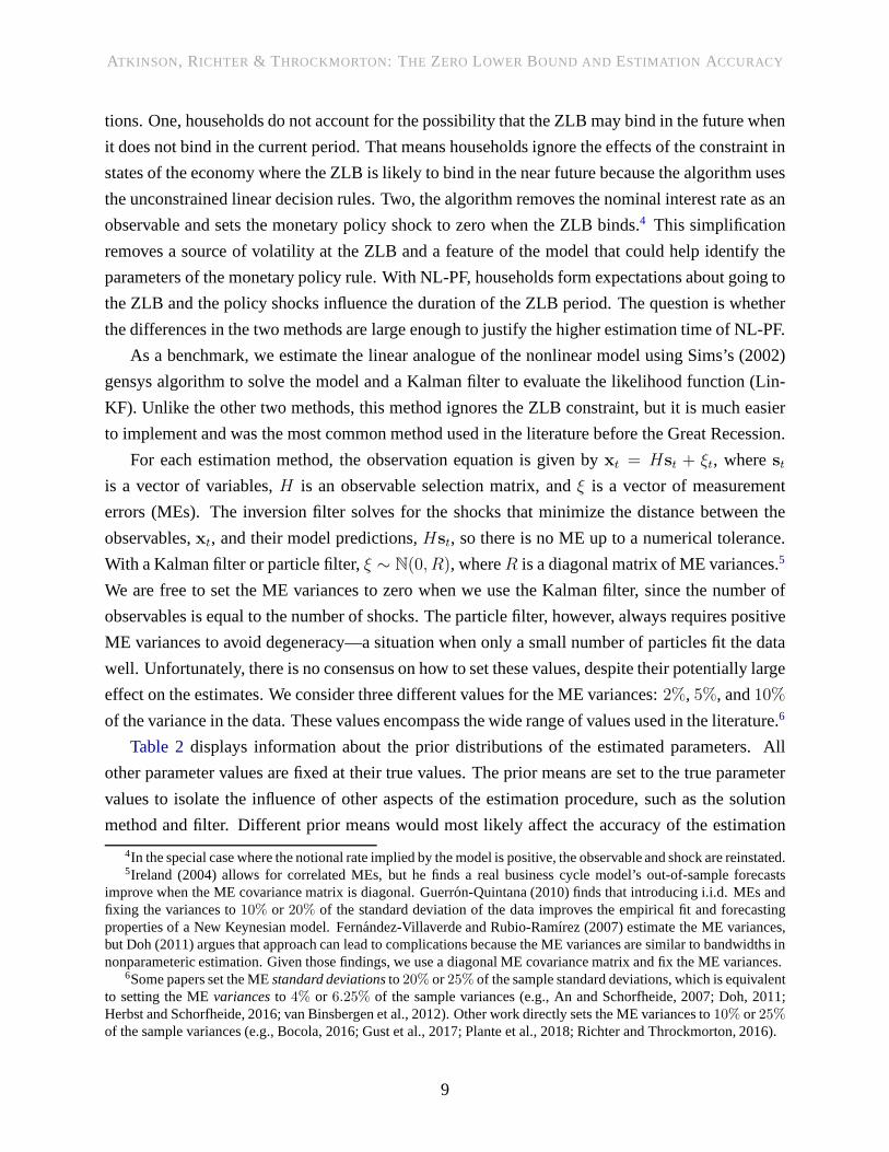
ATKINSON, RICHTER & T HROCKMORTON: THE ZERO LOWER BOUND AND ESTIMATION ACCURACY
tions. One, households do not account for the possibility that the ZLB may bind in the future when
it does not bind in the current period. That means householdsignore the effects of the constraint in
states of the economy where the ZLB is likely to bind in the near future because the algorithm uses
the unconstrained linear decision rules. Two, the algorithm removes the nominal interest rate as an
observable and sets the monetary policy shock to zero when the ZLB binds.4 This simplification
removes a source of volatility at the ZLB and a feature of the model that could help identify the
parameters of the monetary policy rule. With NL-PF, households form expectations about going to
the ZLB and the policy shocks influence the duration of the ZLBperiod. The question is whether
the differences in the two methods are large enough to justify the higher estimation time of NL-PF.
As a benchmark, we estimate the linear analogue of the nonlinear model using Sims’s (2002)
gensys algorithm to solve the model and a Kalman filter to evaluate the likelihood function (Lin-
KF). Unlike the other two methods, this method ignores the ZLB constraint, but it is much easier
to implement and was the most common method used in the literature before the Great Recession.
For each estimation method, the observation equation is given byxt = Hst + ξt, wherestis a vector of variables,H is an observable selection matrix, andξ is a vector of measurement
errors (MEs). The inversion filter solves for the shocks thatminimize the distance between the
observables,xt, and their model predictions,Hst, so there is no ME up to a numerical tolerance.
With a Kalman filter or particle filter,ξ ∼ N(0, R), whereR is a diagonal matrix of ME variances.5
We are free to set the ME variances to zero when we use the Kalman filter, since the number of
observables is equal to the number of shocks. The particle filter, however, always requires positive
ME variances to avoid degeneracy—a situation when only a small number of particles fit the data
well. Unfortunately, there is no consensus on how to set these values, despite their potentially large
effect on the estimates. We consider three different valuesfor the ME variances:2%, 5%, and10%
of the variance in the data. These values encompass the wide range of values used in the literature.6
Table 2displays information about the prior distributions of the estimated parameters. All
other parameter values are fixed at their true values. The prior means are set to the true parameter
values to isolate the influence of other aspects of the estimation procedure, such as the solution
method and filter. Different prior means would most likely affect the accuracy of the estimation
4In the special case where the notional rate implied by the model is positive, the observable and shock are reinstated.5Ireland (2004) allows for correlated MEs, but he finds a real business cycle model’s out-of-sample forecasts
improve when the ME covariance matrix is diagonal. Guerron-Quintana (2010) finds that introducing i.i.d. MEs andfixing the variances to10% or 20% of the standard deviation of the data improves the empiricalfit and forecastingproperties of a New Keynesian model. Fernandez-Villaverde and Rubio-Ramırez (2007) estimate the ME variances,but Doh (2011) argues that approach can lead to complications because the ME variances are similar to bandwidths innonparameteric estimation. Given those findings, we use a diagonal ME covariance matrix and fix the ME variances.
6Some papers set the MEstandard deviationsto20% or25% of the sample standard deviations, which is equivalentto setting the MEvariancesto 4% or 6.25% of the sample variances (e.g., An and Schorfheide, 2007; Doh, 2011;Herbst and Schorfheide, 2016; van Binsbergen et al., 2012).Other work directly sets the ME variances to10% or 25%of the sample variances (e.g., Bocola, 2016; Gust et al., 2017; Plante et al., 2018; Richter and Throckmorton, 2016).
9

ATKINSON, RICHTER & T HROCKMORTON: THE ZERO LOWER BOUND AND ESTIMATION ACCURACY
Parameter Dist. Mean (SD) Parameter Dist. Mean (SD) Parameter Dist. Mean (SD)
ϕp Norm 100 h Beta 0.8 σg IGam 0.005(25) (0.1) (0.005)
φπ Norm 2.0 ρs Beta 0.8 σs IGam 0.005(0.25) (0.1) (0.005)
φy Norm 0.5 ρi Beta 0.8 σi IGam 0.002(0.25) (0.1) (0.002)
Table 2: Prior distributions, means, and standard deviations of the estimated parameters.
and contaminate our results. The prior standard deviations, which are consistent with the values in
the literature, are relatively diffuse to give the algorithm flexibility to search the parameter space.
Our estimation procedure has three stages. First, we conduct a mode search to create an initial
variance-covariance matrix for the estimated parameters.The covariance matrix is based on the
parameters corresponding to the90th percentile of the likelihoods from5,000 draws. Second, we
perform an initial run of the Metropolis-Hastings algorithm with 25,000 draws from the posterior
distribution. We burn off the first5,000 draws and use the remaining draws to update the variance-
covariance matrix from the mode search. Third, we conduct a final run of the Metropolis-Hastings
algorithm. We obtain50,000 draws from the posterior distribution and then record the mean draw.
The algorithm is programmed in Fortran using Open MPI. We runthe datasets in parallel across
several supercomputers. When estimating PW-IF and Lin-KF,each dataset uses a single core. To
estimate NL-PF, each dataset uses16 cores because we parallelize the nonlinear solution across
the nodes in the state space. For example, a supercomputer with 80 cores can simultaneously run
80 PW-IF datasets but only5 NL-PF datasets. To increase the accuracy of the particle filter, we
evaluate the likelihood function on each core. Since each NL-PF dataset uses16 cores, we obtain
16 likelihoods and determine whether to accept or reject a drawbased on the median likelihood.
This step reduces the variance of the likelihoods from seed effects. The filter uses40,000 particles.
NL-PF (16 Cores) PW-IF (1 Core) Lin-KF (1 Core)
0Q 30Q 0Q 30Q 0Q 30Q
Seconds per draw 6.7 8.4 0.035 0.096 0.002 0.002(6.1, 7.9) (7.5, 9.5) (0.031, 0.040) (0.051, 0.135) (0.002, 0.004) (0.001, 0.003)
Hours per dataset 148.8 186.4 0.781 2.137 0.052 0.049(134.9, 176.5) (167.6, 210.7) (0.689, 0.889) (1.133, 3.000) (0.044, 0.089) (0.022, 0.067)
Table 3: Average and(5, 95) percentiles of the estimation times by method and ZLB duration in the data.
Table 3shows the computing times for each estimation method. We approximate the times by
calculating the solution and filter time across the datasetsgiven the parameter estimates. We also
show hours per dataset, which are extrapolated by multiplying seconds per draw by80,000 draws
and dividing by3,600 seconds per hour. We report times for NL-PF, PW-IF, and Lin-KF in datasets
where the ZLB never binds and datasets with one 30 quarter ZLBevent. NL-PF is run on 16 cores
10

ATKINSON, RICHTER & T HROCKMORTON: THE ZERO LOWER BOUND AND ESTIMATION ACCURACY
and the other two methods use a single core. The estimation times depend on the hardware, but
there are two interesting takeaways. One, PW-IF is slightlyslower than Lin-KF, but it only takes a
few hours to run on a single core. Two, NL-PF requires orders of magnitude more time than PW-IF,
which is hard to justify unless there are significant differences in accuracy. However, NL-PF ran in
about a week with16 cores, so it is possible to estimate the fully nonlinear model on a workstation.
4 POSTERIORESTIMATES AND ACCURACY
The section begins by showing the accuracy of the parameter estimates for each estimation method.
We then compare the filtered estimates of the notional interest rate, expected frequency and dura-
tion of the ZLB, responses to a severe recession, and forecasting performance across the methods.
4.1 PARAMETER ESTIMATES We measure parameter accuracy by calculating the normalized
root-mean square-error (NRMSE) for each estimated parameter. For parameterj and estimation
methodh, the error is the difference between the parameter estimatefor datasetk, θj,h,k, and the
true parameter,θj . Therefore, theNRMSE for parameterj and estimation methodh is given by
NRMSEjh = 1
θj
√
1N
∑Nk=1(θj,h,k − θj)
2,
whereN is the number of datasets. TheRMSE is normalized byθj to remove the scale differences.
0Q 6Q 12Q 18Q 24Q 30Q
NL-PF-5% 1.90 1.96 1.99 2.12 2.09 2.08
PW-IF-0% 1.53 1.63 1.71 2.01 1.99 1.91
Lin-KF-0% 1.49 1.62 1.89 2.10 2.30 2.24
Lin-KF-5% 1.88 2.01 2.11 2.27 2.28 2.28
Table 4: Sum of theNRMSE across the estimated parameters. Columns denote the ZLB duration in the data.
Table 4shows the sum of theNRMSE across the parameters. These values provide an aggre-
gate measure of parameter accuracy. The percentage appended to the name of each specification
corresponds to the size of the ME variances. The estimates from datasets without a ZLB event
show how well each specification performs without any influence from the ZLB constraint. With
these datasets, PW-IF-0% and Lin-KF-0% have roughly the same accuracy since the solution meth-
ods are identical when the ZLB does not bind. Interestingly,both of those specifications are more
accurate than NL-PF-5%. The results for Lin-KF-5% show the lower accuracy of NL-PF-5% is
driven by positive ME variances and that the ZLB is the only important nonlinearity in the model.
Comparing the columns for each method shows the effects of the ZLB duration in the data.
When the ZLB binds, it reduces the accuracy of every specification and accuracy typically dimin-
ishes as the ZLB event lengthens. Lengthening the ZLB event in the data has the smallest effect on
11
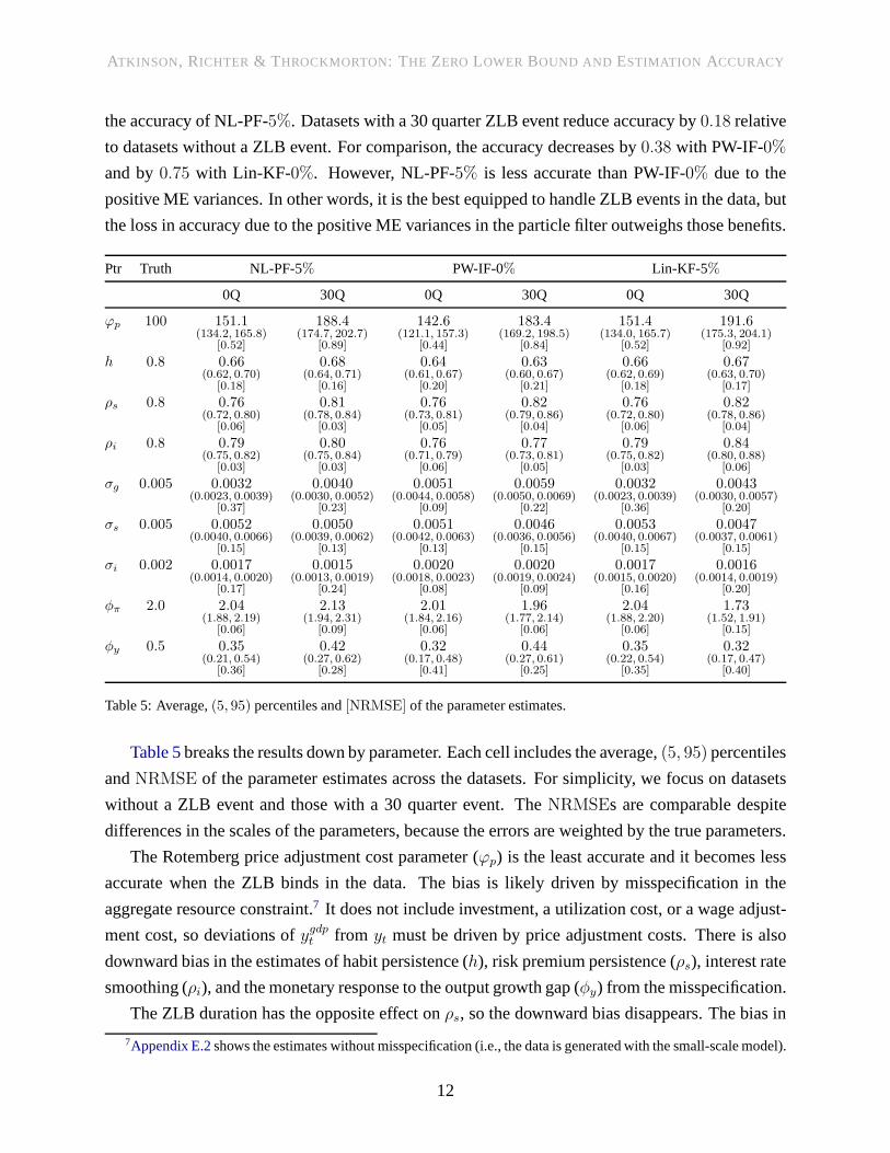
ATKINSON, RICHTER & T HROCKMORTON: THE ZERO LOWER BOUND AND ESTIMATION ACCURACY
the accuracy of NL-PF-5%. Datasets with a 30 quarter ZLB event reduce accuracy by0.18 relative
to datasets without a ZLB event. For comparison, the accuracy decreases by0.38 with PW-IF-0%
and by0.75 with Lin-KF-0%. However, NL-PF-5% is less accurate than PW-IF-0% due to the
positive ME variances. In other words, it is the best equipped to handle ZLB events in the data, but
the loss in accuracy due to the positive ME variances in the particle filter outweighs those benefits.
Ptr Truth NL-PF-5% PW-IF-0% Lin-KF-5%
0Q 30Q 0Q 30Q 0Q 30Q
ϕp 100 151.1 188.4 142.6 183.4 151.4 191.6(134.2, 165.8) (174.7, 202.7) (121.1, 157.3) (169.2, 198.5) (134.0, 165.7) (175.3, 204.1)
[0.52] [0.89] [0.44] [0.84] [0.52] [0.92]
h 0.8 0.66 0.68 0.64 0.63 0.66 0.67(0.62, 0.70) (0.64, 0.71) (0.61, 0.67) (0.60, 0.67) (0.62, 0.69) (0.63, 0.70)
[0.18] [0.16] [0.20] [0.21] [0.18] [0.17]
ρs 0.8 0.76 0.81 0.76 0.82 0.76 0.82(0.72, 0.80) (0.78, 0.84) (0.73, 0.81) (0.79, 0.86) (0.72, 0.80) (0.78, 0.86)
[0.06] [0.03] [0.05] [0.04] [0.06] [0.04]
ρi 0.8 0.79 0.80 0.76 0.77 0.79 0.84(0.75, 0.82) (0.75, 0.84) (0.71, 0.79) (0.73, 0.81) (0.75, 0.82) (0.80, 0.88)
[0.03] [0.03] [0.06] [0.05] [0.03] [0.06]
σg 0.005 0.0032 0.0040 0.0051 0.0059 0.0032 0.0043(0.0023, 0.0039) (0.0030, 0.0052) (0.0044, 0.0058) (0.0050, 0.0069) (0.0023, 0.0039) (0.0030, 0.0057)
[0.37] [0.23] [0.09] [0.22] [0.36] [0.20]
σs 0.005 0.0052 0.0050 0.0051 0.0046 0.0053 0.0047(0.0040, 0.0066) (0.0039, 0.0062) (0.0042, 0.0063) (0.0036, 0.0056) (0.0040, 0.0067) (0.0037, 0.0061)
[0.15] [0.13] [0.13] [0.15] [0.15] [0.15]
σi 0.002 0.0017 0.0015 0.0020 0.0020 0.0017 0.0016(0.0014, 0.0020) (0.0013, 0.0019) (0.0018, 0.0023) (0.0019, 0.0024) (0.0015, 0.0020) (0.0014, 0.0019)
[0.17] [0.24] [0.08] [0.09] [0.16] [0.20]
φπ 2.0 2.04 2.13 2.01 1.96 2.04 1.73(1.88, 2.19) (1.94, 2.31) (1.84, 2.16) (1.77, 2.14) (1.88, 2.20) (1.52, 1.91)
[0.06] [0.09] [0.06] [0.06] [0.06] [0.15]
φy 0.5 0.35 0.42 0.32 0.44 0.35 0.32(0.21, 0.54) (0.27, 0.62) (0.17, 0.48) (0.27, 0.61) (0.22, 0.54) (0.17, 0.47)
[0.36] [0.28] [0.41] [0.25] [0.35] [0.40]
Table 5: Average,(5, 95) percentiles and[NRMSE] of the parameter estimates.
Table 5breaks the results down by parameter. Each cell includes theaverage,(5, 95) percentiles
andNRMSE of the parameter estimates across the datasets. For simplicity, we focus on datasets
without a ZLB event and those with a 30 quarter event. TheNRMSEs are comparable despite
differences in the scales of the parameters, because the errors are weighted by the true parameters.
The Rotemberg price adjustment cost parameter (ϕp) is the least accurate and it becomes less
accurate when the ZLB binds in the data. The bias is likely driven by misspecification in the
aggregate resource constraint.7 It does not include investment, a utilization cost, or a wageadjust-
ment cost, so deviations ofygdpt from yt must be driven by price adjustment costs. There is also
downward bias in the estimates of habit persistence (h), risk premium persistence (ρs), interest rate
smoothing (ρi), and the monetary response to the output growth gap (φy) from the misspecification.
The ZLB duration has the opposite effect onρs, so the downward bias disappears. The bias in
7Appendix E.2shows the estimates without misspecification (i.e., the data is generated with the small-scale model).
12

ATKINSON, RICHTER & T HROCKMORTON: THE ZERO LOWER BOUND AND ESTIMATION ACCURACY
the NL-PF-5% estimates of the technology growth and monetary policy shock standard deviations
(σg andσi) is due to the positive ME variances in the filter, as Lin-KF-5% produces identical es-
timates. The importance of the ME variances is likely drivenby the filter ascribing large shocks
to ME rather than the structural shocks, reducing their estimated volatility. Therefore, it is notable
that NL-PF-5% is the most accurate in estimating the parameters that drivethe risk-premium shock
(ρs andσs), and long ZLB events do not make them less accurate. Overall, the decreases in accu-
racy due to the ZLB are largely driven by a single parameter (ϕp) and for many of the parameters
accuracy is higher in datasets with a 30 quarter ZLB event than datasets where the ZLB never binds.
Ptr Truth NL-PF-2% NL-PF-5% NL-PF-10%
0Q 30Q 0Q 30Q 0Q 30Q
ϕp 100 150.2 192.0 151.1 188.4 149.5 182.7(133.5, 165.3) (176.5, 207.1) (134.2, 165.8) (174.7, 202.7) (132.6, 163.8) (168.6, 197.3)
[0.51] [0.93] [0.52] [0.89] [0.50] [0.83]
h 0.8 0.66 0.67 0.66 0.68 0.66 0.68(0.62, 0.69) (0.64, 0.71) (0.62, 0.70) (0.64, 0.71) (0.61, 0.70) (0.65, 0.72)
[0.18] [0.17] [0.18] [0.16] [0.17] [0.15]
ρs 0.8 0.76 0.81 0.76 0.81 0.76 0.81(0.71, 0.79) (0.78, 0.84) (0.72, 0.80) (0.78, 0.84) (0.72, 0.79) (0.79, 0.85)
[0.06] [0.03] [0.06] [0.03] [0.06] [0.03]
ρi 0.8 0.77 0.79 0.79 0.80 0.80 0.81(0.73, 0.80) (0.75, 0.83) (0.75, 0.82) (0.75, 0.84) (0.77, 0.84) (0.76, 0.85)
[0.05] [0.03] [0.03] [0.03] [0.03] [0.03]
σg 0.005 0.0038 0.0043 0.0032 0.0040 0.0027 0.0038(0.0031, 0.0043) (0.0035, 0.0052) (0.0023, 0.0039) (0.0030, 0.0052) (0.0020, 0.0035) (0.0025, 0.0050)
[0.25] [0.18] [0.37] [0.23] [0.46] [0.28]
σs 0.005 0.0052 0.0051 0.0052 0.0050 0.0051 0.0049(0.0039, 0.0065) (0.0040, 0.0061) (0.0040, 0.0066) (0.0039, 0.0062) (0.0041, 0.0065) (0.0037, 0.0061)
[0.15] [0.13] [0.15] [0.13] [0.14] [0.14]
σi 0.002 0.0019 0.0018 0.0017 0.0015 0.0015 0.0013(0.0017, 0.0021) (0.0016, 0.0021) (0.0014, 0.0020) (0.0013, 0.0019) (0.0012, 0.0018) (0.0011, 0.0017)
[0.10] [0.14] [0.17] [0.24] [0.25] [0.34]
φπ 2.0 2.01 2.14 2.04 2.13 2.06 2.12(1.84, 2.16) (1.96, 2.31) (1.88, 2.19) (1.94, 2.31) (1.89, 2.21) (1.92, 2.28)
[0.06] [0.09] [0.06] [0.09] [0.07] [0.08]
φy 0.5 0.31 0.39 0.35 0.42 0.41 0.46(0.18, 0.48) (0.24, 0.60) (0.21, 0.54) (0.27, 0.62) (0.26, 0.59) (0.30, 0.66)
[0.42] [0.32] [0.36] [0.28] [0.27] [0.24]
Σ [1.79] [2.01] [1.90] [2.08] [1.95] [2.13]
Table 6: Average,(5, 95) percentiles and[NRMSE] of the parameter estimates.Σ is sum of theNRMSE.
ME Variances Table 6shows the parameter estimates andNRMSEs for NL-PF with three dif-
ferent ME variances:2%, 5% (baseline), and10%. If there was no misspecificiation, it would be
obvious that lower ME variances would increase accuracy until the effective sample size in the
particle filter became too small. In our setup, the presence of misspecification creates a potential
tradeoff. On the one hand, lower ME variances force the modelto match sharp swings in the data,
which could help identify the parameters. On the other hand,higher ME variances give the model a
degree of freedom to account for important discrepancies between the estimated model and the data
generating process (e.g., the aggregate resource constraint), which could decrease parameter bias.
13
ATKINSON, RICHTER & T HROCKMORTON: THE ZERO LOWER BOUND AND ESTIMATION ACCURACY
We find smaller ME variances reduce the sum of theNRMSE across the parameters. Forσg
andσi, higher ME variances push the estimates lower, away from thetrue value. Once again, this
result is likely driven by the filter incorrectly ascribing movements in the data to ME rather than
the structural shocks. This loss in accuracy as the ME variances increase is partially offset by the
increase in the accuracy of most other parameters. Estimates ofφy with all datasets and estimates
of ϕp with datasets where the ZLB binds for 30 quarters improve themost. These parameters are
tightly linked to real GDP and the aggregate resource constraint, which is a key misspecification
that is compensated for with higher ME. These results show that ME variances are important for
accuracy. In some cases, they may compensate for model misspecification and enable use of the
particle filter. In our setup, however, positive ME variances have a net negative effect on accuracy.
4.2 NOTIONAL INTEREST RATE ESTIMATES We measure the accuracy of the notional rate by
calculating the averageRMSE across periods when the ZLB binds. For periodt and estimation
methodh, the error is the difference between the filtered notional rate based on the parameter
estimates for datasetk, ınt,h,k, and the true notional rate,ınt . TheRMSE for methodh is given by
RMSEin
h =√
1N
1τ
∑Nk=1
∑t+τ−1j=t (ınj,h,k − ınj )
2,
wheret is the first period the ZLB binds andτ is the duration of the ZLB event. There is no reason
to normalize theRMSE since the units are the same across periods and we do not sum across states.
Estimates of the notional interest rate are of keen interestto policymakers for two key rea-
sons. One, they summarize the severity of the recession and the nominal interest rate policymakers
would like to set in the absence of the ZLB, which help inform decisions about implementing un-
conventional monetary policy. Two, estimates of the notional rate help determine how long the
ZLB is expected to bind, which is necessary to issue forward guidance. The notional rate is also
the only latent endogenous state variable in the model that is not directly linked to an observable.
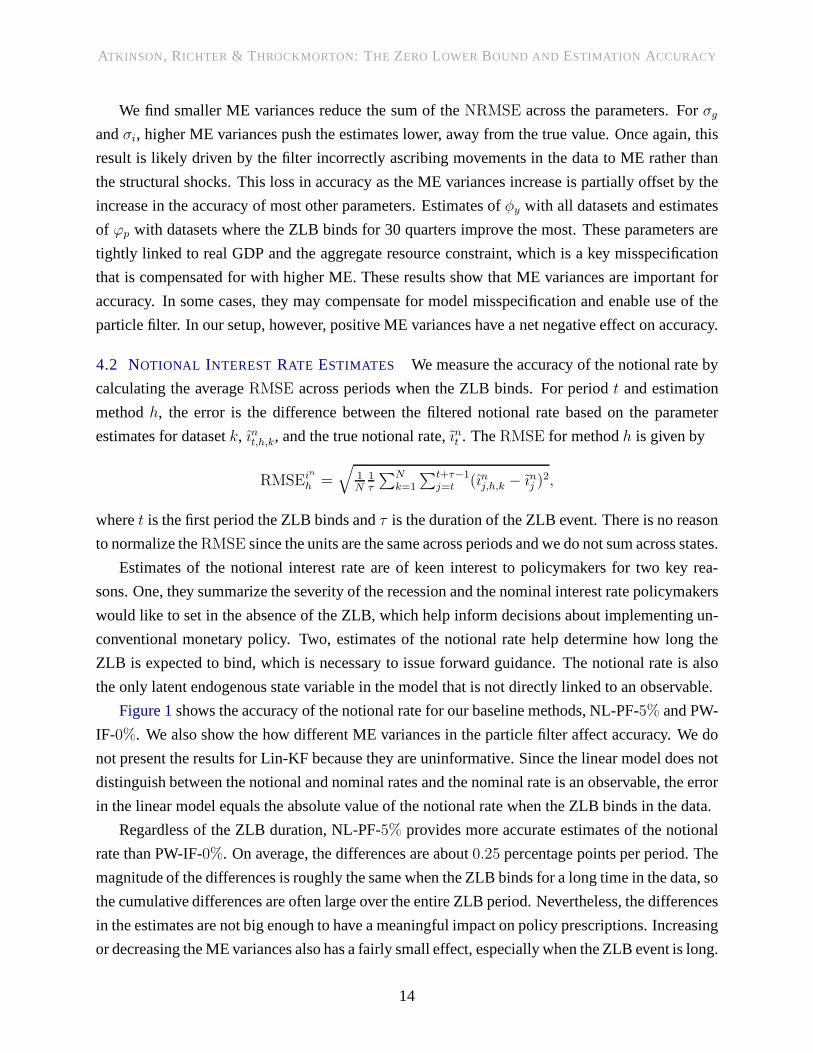
Figure 1shows the accuracy of the notional rate for our baseline methods, NL-PF-5% and PW-
IF-0%. We also show the how different ME variances in the particle filter affect accuracy. We do
not present the results for Lin-KF because they are uninformative. Since the linear model does not
distinguish between the notional and nominal rates and the nominal rate is an observable, the error
in the linear model equals the absolute value of the notionalrate when the ZLB binds in the data.
Regardless of the ZLB duration, NL-PF-5% provides more accurate estimates of the notional
rate than PW-IF-0%. On average, the differences are about0.25 percentage points per period. The
magnitude of the differences is roughly the same when the ZLBbinds for a long time in the data, so
the cumulative differences are often large over the entire ZLB period. Nevertheless, the differences
in the estimates are not big enough to have a meaningful impact on policy prescriptions. Increasing
or decreasing the ME variances also has a fairly small effect, especially when the ZLB event is long.
14
ATKINSON, RICHTER & T HROCKMORTON: THE ZERO LOWER BOUND AND ESTIMATION ACCURACY
6Q 12Q 18Q 24Q 30Q0
0.25
0.5
0.75
1
1.25
1.5
1.75
Figure 1:RMSE of the notional interest rate across ZLB durations in the data. Rates are net annualized percentages.
4.3 EXPECTED ZLB DURATION AND PROBABILITY In addition to estimates of the notional in-
terest rate, two commonly referenced statistics in the literature are the expected duration and prob-
ability of the ZLB constraint. These statistics determine the impact of a ZLB event in the model
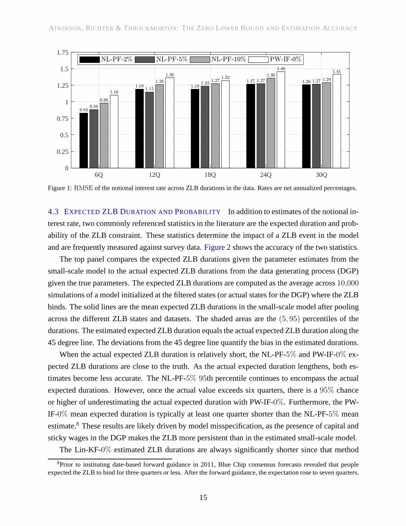
and are frequently measured against survey data.Figure 2shows the accuracy of the two statistics.
The top panel compares the expected ZLB durations given the parameter estimates from the
small-scale model to the actual expected ZLB durations fromthe data generating process (DGP)
given the true parameters. The expected ZLB durations are computed as the average across10,000
simulations of a model initialized at the filtered states (oractual states for the DGP) where the ZLB
binds. The solid lines are the mean expected ZLB durations inthe small-scale model after pooling
across the different ZLB states and datasets. The shaded areas are the(5, 95) percentiles of the
durations. The estimated expected ZLB duration equals the actual expected ZLB duration along the
45 degree line. The deviations from the 45 degree line quantify the bias in the estimated durations.
When the actual expected ZLB duration is relatively short, the NL-PF-5% and PW-IF-0% ex-
pected ZLB durations are close to the truth. As the actual expected duration lengthens, both es-
timates become less accurate. The NL-PF-5% 95th percentile continues to encompass the actual
expected durations. However, once the actual value exceedssix quarters, there is a95% chance
or higher of underestimating the actual expected duration with PW-IF-0%. Furthermore, the PW-
IF-0% mean expected duration is typically at least one quarter shorter than the NL-PF-5% mean
estimate.8 These results are likely driven by model misspecification, as the presence of capital and
sticky wages in the DGP makes the ZLB more persistent than in the estimated small-scale model.
The Lin-KF-0% estimated ZLB durations are always significantly shorter since that method
8Prior to instituting date-based forward guidance in 2011, Blue Chip consensus forecasts revealed that peopleexpected the ZLB to bind for three quarters or less. After theforward guidance, the expectation rose to seven quarters.
15

ATKINSON, RICHTER & T HROCKMORTON: THE ZERO LOWER BOUND AND ESTIMATION ACCURACY
(a) Estimated vs. Actual Expected ZLB Durations
2 4 6 8 10 12
2
4
6
8
10
12
2 4 6 8 10 12
2
4
6
8
10
12
2 4 6 8 10 12
2
4
6
8
10
12
(b) Estimated vs. Actual Probability of a 4 Quarter or LongerZLB Event
0 0.1 0.2 0.3 0.4 0.50
0.1
0.2
0.3
0.4
0.5
0 0.1 0.2 0.3 0.4 0.50
0.1
0.2
0.3
0.4
0.5
Figure 2: Estimated and actual ZLB statistics. The solid lines are mean estimates and the shaded areas capture the(5, 95) percentiles across the datasets. The dashed line shows where the estimated values would equal the actual values.
does not permit a negative notional rate when filtering the data. The only instance when Lin-
KF-0% produces an expected ZLB duration beyond one year is when theeconomy is in a severe
downturn and the actual expected duration is extremely long. The Lin-KF-0% estimates are a lower
bound on the PW-IF-0% estimates since the solutions are identical when the ZLB does not bind.
The bottom panel is constructed in a similar way as the top panel except the horizontal and
vertical axes correspond to the actual and estimated probability of a ZLB event that lasts for at
least four quarters. The probability is calculated in all periods where the ZLB does not bind in the
data. We do not show the results for Lin-KF-0% because the probability of a four quarter ZLB event
is always near zero. NL-PF-5% and PW-IF-0% underestimate the true probability, but the mean
NL-PF-5% estimates are slightly closer to the actual probabilities and the95th percentile almost
encompasses the truth. These results illustrate the precautionary savings effects of the ZLB, which
are not captured by PW-IF-0%. However, they do not provide overwhelming support for NL-PF-
5%, and changing the ME variances in the particle filter has no discernable effect on the results.
16

ATKINSON, RICHTER & T HROCKMORTON: THE ZERO LOWER BOUND AND ESTIMATION ACCURACY
0 2 4 6 8 10 12 14 16 18 20-10
-7.5
-5
-2.5
0
2.5
5
0 2 4 6 8 10 12 14 16 18 20-10
-7.5
-5
-2.5
0
2.5
5
0 2 4 6 8 10 12 14 16 18 20-4
-3
-2
-1
0
1
2
0 2 4 6 8 10 12 14 16 18 20-4
-3
-2
-1
0
1
2
0 2 4 6 8 10 12 14 16 18 20-6
-4
-2
0
2
4
0 2 4 6 8 10 12 14 16 18 20-6
-4
-2
0
2
4
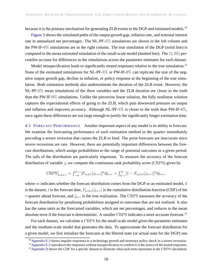
Figure 3: Recession responses. The solid line is the true simulation, the dashed line is the mean estimated simulation,and the shaded area contains the(5, 95) percentiles across the datasets. The simulations are initialized in steady stateand followed by four1.5 standard deviation positive risk premium shocks. All values are net annualized percentages.
4.4 RECESSIONRESPONSES To illustrate the economic implications of the differencesin ac-
curacy, we compare simulations of the small-scale model given our parameter estimates to simula-
tions of the DGP given the true parameters. The simulations are initialized in steady state and fol-
lowed by four consecutive1.5 standard deviation positive risk premium shocks, which generates a
10 quarter ZLB event in the DGP.9 A risk premium shock is a proxy for a change in demand because
it affects households’ consumption and saving decisions. Positive shocks cause households to post-
pone consumption to future periods, which reduces current output growth. We focus on this shock
9The simulations are reflective of the Great Recession. The current Congressional Budget Office estimate of theoutput gap in 2009Q2 is−5.9%, roughly equivalent to the output (level) gap in the true simulation in the fourth period.
17
ATKINSON, RICHTER & T HROCKMORTON: THE ZERO LOWER BOUND AND ESTIMATION ACCURACY
because it is the primary mechanism for generating ZLB events in the DGP and estimated models.10
Figure 3shows the simulated paths of the output growth gap, inflationrate, and notional interest
rate in annualized net percentages. The NL-PF-5% simulations are shown in the left column and
the PW-IF-0% simulations are in the right column. The true simulation of the DGP (solid line) is
compared to the mean estimated simulation of the small-scale model (dashed line). The(5, 95) per-
centiles account for differences in the simulations acrossthe parameter estimates for each dataset.
Model misspecification leads to significantly muted responses relative to the true simulation.11
None of the estimated simulations for NL-PF-5% or PW-IF-0% can replicate the size of the neg-
ative output growth gap, decline in inflation, or policy response at the beginning of the true simu-
lation. Both estimation methods also underestimate the duration of the ZLB event. However, the
NL-PF-5% mean simulations of the three variables and the ZLB durationare closer to the truth
than the PW-IF-0% simulations. Unlike the piecewise linear solution, the fully nonlinear solution
captures the expectational effects of going to the ZLB, which puts downward pressure on output
and inflation and improves accuracy. Although NL-PF-5% is closer to the truth than PW-IF-0%,
once again these differences are not large enough to justifythe significantly longer estimation time.
4.5 FORECASTPERFORMANCE Another important aspect of any model is its ability to forecast.
We examine the forecasting performance of each estimation method in the quarter immediately
preceding a severe recession that causes the ZLB to bind. Thepoint forecasts are inaccurate since
severe recessions are rare. However, there are potentiallyimportant differences between the fore-
cast distributions, which assign probabilities to the range of potential outcomes in a given period.
The tails of the distribution are particularly important. To measure the accuracy of the forecast
distribution of variablej, we compute the continuous rank probability score (CRPS) given by
CRPSjm,k,t,τ =
∫ t+τ
−∞[Fm,k,t(jt+τ )]
2djt+τ +∫
∞
t+τ[1− Fm,k,t(jt+τ )]
2djt+τ ,
wherem indicates whether the forecast distribution comes from theDGP or an estimated model,k
is the dataset,t is the forecast date,Fm,k,t(jt+τ ) is the cumulative distribution function (CDF) of the
τ -quarter ahead forecast, andt+τ is the true realization. TheCRPS measures the accuracy of the
forecast distribution by penalizing probabilities assigned to outcomes that are not realized. It also
has the same units as the forecasted variables, which are netpercentages, and reduces to the mean
absolute error if the forecast is deterministic. A smallerCRPS indicates a more accurate forecast.12
For each dataset, we calculate aCRPS for the small-scale model given the parameter estimates
and the medium-scale model that generates the data. To approximate the forecast distribution for
a given model, we first initialize the forecasts at the filtered state (or actual state for the DGP) one
10Appendix E.3shows impulse responses to a technology growth and monetarypolicy shock in a severe recession.11Appendix E.2reproduces the responses without misspecification to confirm it is the source of the muted responses.12Appendix Dshows the CDF for a specific dataset to illustrate what each term represents in theCRPS calculation.
18
ATKINSON, RICHTER & T HROCKMORTON: THE ZERO LOWER BOUND AND ESTIMATION ACCURACY
quarter before the ZLB binds in the data. Then we draw random shocks and simulate the model
for 8 quarters,10,000 times. Using the simulations, we approximate the CDF of the forecast dis-
tribution 8-quarters ahead.13 Finally, we average theCRPS for a given model across the datasets.
6Q 12Q 18Q 24Q 30Q0
0.5
1
1.5
2
0
0.5
1
1.5
2
0
1
2
3
4
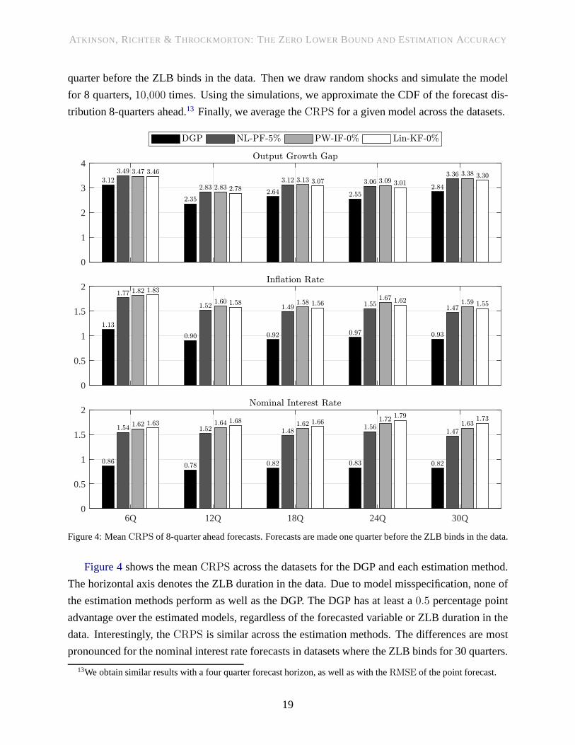
Figure 4: MeanCRPS of 8-quarter ahead forecasts. Forecasts are made one quarter before the ZLB binds in the data.
Figure 4shows the meanCRPS across the datasets for the DGP and each estimation method.
The horizontal axis denotes the ZLB duration in the data. Dueto model misspecification, none of
the estimation methods perform as well as the DGP. The DGP hasat least a0.5 percentage point
advantage over the estimated models, regardless of the forecasted variable or ZLB duration in the
data. Interestingly, theCRPS is similar across the estimation methods. The differences are most
pronounced for the nominal interest rate forecasts in datasets where the ZLB binds for 30 quarters.
13We obtain similar results with a four quarter forecast horizon, as well as with theRMSE of the point forecast.
19

ATKINSON, RICHTER & T HROCKMORTON: THE ZERO LOWER BOUND AND ESTIMATION ACCURACY
The NL-PF-5% CRPS is only 179% of the DGPCRPS, compared to199% for PW-IF-0% and
211% for Lin-KF-0%. The NL-PF-5% forecasts of the inflation rate are also consistently more
accurate than the other estimation methods. However, in allcases the differences in accuracy are
small relative to the DGP. These findings are consistent withour previous results. NL-PF-5% has
an advantage over PW-IF-0%, but it is never large enough to justify the higher computational costs.
5 CONCLUSION
During the Great Recession, many central banks lowered their policy rate to its ZLB, creating
a kink in their policy rule and calling into question linear estimation methods. There are two
promising alternatives: estimate a fully nonlinear model that accounts for the expectational effects
of going to the ZLB or a piecewise linear model that is faster but ignores the expectational effects.
This paper examines whether the differences in accuracy justify the longer estimation time. Based
on our estimates with both methods, we find the answer is no, regardless of the ZLB duration in
the data. Model misspecification, however, biases the parameter estimates and creates significant
differences between the predictions of the two estimated models and the data generating process.
Our results indicate that PW-IF is an excellent substitute for NL-PF and that it is more beneficial
to reduce misspecification by estimating a richer piecewiselinear model than a simpler but prop-
erly solved nonlinear model when examining the empirical implications of the ZLB constraint.14
The nonlinear model has the advantage that it is more versatile. While the piecewise linear and
nonlinear models can handle any combination of occasionally binding constraints, only the non-
linear model can account for other nonlinear features emphasized in the literature (e.g., stochastic
volatility, asymmetric adjustment costs, non-Gaussian shocks, search frictions, time-varying pol-
icy rules, changes in steady states). Our results will also serve as an important starting point for
research that explores these nonlinear features or makes advances in nonlinear estimation methods.
REFERENCES
AN, S. AND F. SCHORFHEIDE (2007): “Bayesian Analysis of DSGE Models,”Econometric
Reviews, 26, 113–172,https://doi.org/10.1080/07474930701220071.
ARUOBA, S., P. CUBA-BORDA, AND F. SCHORFHEIDE (2018): “Macroeconomic Dynamics
Near the ZLB: A Tale of Two Countries,”The Review of Economic Studies, 85, 87–118,
https://doi.org/10.1093/restud/rdx027.
BOCOLA, L. (2016): “The Pass-Through of Sovereign Risk,”Journal of Political Economy, 124,
879–926,https://doi.org/10.1086/686734.
14Appendix E.1shows the estimates from the piecewise linear model after reducing the amount of misspecification.
20
ATKINSON, RICHTER & T HROCKMORTON: THE ZERO LOWER BOUND AND ESTIMATION ACCURACY
CANOVA , F., F. FERRONI, AND C. MATTHES (2014): “Choosing The Variables To Estimate
Singular Dsge Models,”Journal of Applied Econometrics, 29, 1099–1117,
https://doi.org/10.1002/jae.2414.CHUGH, S. K. (2006): “Optimal Fiscal and Monetary Policy with Sticky Wages and Sticky
Prices,”Review of Economic Dynamics, 9, 683–714,https://doi.org/10.1016/j.red.2006.07.001.COLEMAN , II, W. J. (1991): “Equilibrium in a Production Economy withan Income Tax,”
Econometrica, 59, 1091–1104,https://doi.org/10.2307/2938175.CUBA-BORDA, P., L. GUERRIERI, M. IACOVIELLO , AND M. ZHONG (2017): “Likelihood
Evaluation of Models with Occasionally Binding Constraints,” Federal Reserve Board.DOH, T. (2011): “Yield Curve in an Estimated Nonlinear Macro Model,” Journal of Economic
Dynamics and Control, 35, 1229 – 1244,https://doi.org/10.1016/j.jedc.2011.03.003.FAIR, R. C.AND J. B. TAYLOR (1983): “Solution and Maximum Likelihood Estimation of
Dynamic Nonlinear Rational Expectations Models,”Econometrica, 51, 1169–1185,
https://doi.org/10.2307/1912057.FERNALD, J. G. (2012): “A Quarterly, Utilization-Adjusted Series on Total Factor Productivity,”
Federal Reserve Bank of San Francisco Working Paper 2012-19.FERNANDEZ-V ILLAVERDE , J., G. GORDON, P. GUERRON-QUINTANA , AND J. F.
RUBIO-RAM IREZ (2015): “Nonlinear Adventures at the Zero Lower Bound,”Journal of
Economic Dynamics and Control, 57, 182–204,https://doi.org/10.1016/j.jedc.2015.05.014.FERNANDEZ-V ILLAVERDE , J. AND J. F. RUBIO-RAM IREZ (2005): “Estimating Dynamic
Equilibrium Economies: Linear versus Nonlinear Likelihood,” Journal of Applied
Econometrics, 20, 891–910,https://doi.org/10.1002/jae.814.——— (2007): “Estimating Macroeconomic Models: A Likelihood Approach,”The Review of
Economic Studies, 74, 1059–1087,https://doi.org/10.1111/j.1467-937X.2007.00437.x.GAVIN , W. T., B. D. KEEN, A. W. RICHTER, AND N. A. THROCKMORTON (2015): “The Zero
Lower Bound, the Dual Mandate, and Unconventional Dynamics,” Journal of Economic
Dynamics and Control, 55, 14–38,https://doi.org/10.1016/j.jedc.2015.03.007.GORDON, N. J., D. J. SALMOND , AND A. F. M. SMITH (1993): “Novel Approach to
Nonlinear/Non-Gaussian Bayesian State Estimation,”IEE Proceedings F - Radar and Signal
Processing, 140, 107–113,https://doi.org/10.1049/ip-f-2.1993.0015.GUERRIERI, L. AND M. IACOVIELLO (2015): “OccBin: A Toolkit for Solving Dynamic Models
with Occasionally Binding Constraints Easily,”Journal of Monetary Economics, 70, 22–38,
https://doi.org/10.1016/j.jmoneco.2014.08.005.——— (2017): “Collateral Constraints and Macroeconomic Asymmetries,”Journal of Monetary
Economics, 90, 28–49,https://doi.org/10.1016/j.jmoneco.2017.06.004.GUERRON-QUINTANA , P. A. (2010): “What You Match Does Matter: The Effects of Data on
DSGE Estimation,”Journal of Applied Econometrics, 25, 774–804,
https://doi.org/10.1002/jae.1106.
21

ATKINSON, RICHTER & T HROCKMORTON: THE ZERO LOWER BOUND AND ESTIMATION ACCURACY
GUST, C., E. HERBST, D. LOPEZ-SALIDO , AND M. E. SMITH (2017): “The Empirical
Implications of the Interest-Rate Lower Bound,”American Economic Review, 107, 1971–2006,
https://doi.org/10.1257/aer.20121437.
HERBST, E. AND F. SCHORFHEIDE (2018): “Tempered Particle Filtering,”Journal of
Econometrics, forthcoming,https://doi.org/10.1016/j.jeconom.2018.11.003.
HERBST, E. P.AND F. SCHORFHEIDE (2016):Bayesian Estimation of DSGE Models, Princeton,
NJ: Princeton University Press.
HIROSE, Y. AND A. INOUE (2016): “The Zero Lower Bound and Parameter Bias in an Estimated
DSGE Model,”Journal of Applied Econometrics, 31, 630–651,
https://doi.org/10.1002/jae.2447.
HIROSE, Y. AND T. SUNAKAWA (2015): “Parameter Bias in an Estimated DSGE Model: Does
Nonlinearity Mattter?” Centre for Applied Macroceonomic Analysis Working Paper 46/2015.
I IBOSHI, H., M. SHINTANI , AND K. UEDA (2018): “Estimating a Nonlinear New Keynesian
Model with a Zero Lower Bound for Japan,” Tokyo Center for Economic Research Working
Paper E-120.
IRELAND, P. N. (2004): “A Method for Taking Models to the Data,”Journal of Economic
Dynamics and Control, 28, 1205–1226,https://doi.org/10.1016/S0165-1889(03)00080-0.
KEEN, B. D., A. W. RICHTER, AND N. A. THROCKMORTON (2017): “Forward Guidance and
the State of the Economy,”Economic Inquiry, 55, 1593–1624,
https://doi.org/10.1111/ecin.12466.
K ITAGAWA , G. (1996): “Monte Carlo Filter and Smoother for Non-Gaussian Nonlinear State
Space Models,”Journal of Computational and Graphical Statistics, 5, pp. 1–25,
https://doi.org/10.2307/1390750.
KOOP, G., M. H. PESARAN, AND S. M. POTTER (1996): “Impulse Response Analysis in
Nonlinear Multivariate Models,”Journal of Econometrics, 74, 119–147,
https://doi.org/10.1016/0304-4076(95)01753-4.
KOPECKY, K. AND R. SUEN (2010): “Finite State Markov-chain Approximations to Highly
Persistent Processes,”Review of Economic Dynamics, 13, 701–714,
https://doi.org/10.1016/j.red.2010.02.002.
LAUBACH , T. AND J. C. WILLIAMS (2016): “Measuring the Natural Rate of Interest Redux,”
Finance and Economics Discussion Series 2016-011.
MERTENS, K. AND M. O. RAVN (2014): “Fiscal Policy in an Expectations Driven Liquidity
Trap,” The Review of Economic Studies, 81, 1637–1667,https://doi.org/10.1093/restud/rdu016.
NAKATA , T. (2017): “Uncertainty at the Zero Lower Bound,”American Economic Journal:
Macroeconomics, 9, 186–221,https://doi.org/10.1257/mac.20140253.
NAKOV, A. (2008): “Optimal and Simple Monetary Policy Rules with Zero Floor on the Nominal
Interest Rate,”International Journal of Central Banking, 4, 73–127.
22

ATKINSON, RICHTER & T HROCKMORTON: THE ZERO LOWER BOUND AND ESTIMATION ACCURACY
NGO, P. V. (2014): “Optimal Discretionary Monetary Policy in a Micro-Founded Model with a
Zero Lower Bound on Nominal Interest Rate,”Journal of Economic Dynamics and Control, 45,
44–65,https://doi.org/10.1016/j.jedc.2014.05.010.
OTROK, C. (2001): “On Measuring the Welfare Cost of Business Cycles,” Journal of Monetary
Economics, 47, 61–92,https://doi.org/10.1016/S0304-3932(00)00052-0.
PETERMAN, W. B. (2016): “Reconciling Micro and Macro Estimates of theFrisch Labor Supply
Elasticity,” Economic Inquiry, 54, 100–120,https://doi.org/10.1111/ecin.12252.
PLANTE , M., A. W. RICHTER, AND N. A. THROCKMORTON (2018): “The Zero Lower Bound
and Endogenous Uncertainty,”Economic Journal, 128, 1730–1757,
https://doi.org/10.1111/ecoj.12445.
RICHTER, A. W. AND N. A. THROCKMORTON (2015): “The Zero Lower Bound: Frequency,
Duration, and Numerical Convergence,”B.E. Journal of Macroeconomics, 15, 157–182,
https://doi.org/10.1515/bejm-2013-0185.
——— (2016): “Is Rotemberg Pricing Justified by Macro Data?”Economics Letters, 149, 44–48,
https://doi.org/10.1016/j.econlet.2016.10.011.
RICHTER, A. W., N. A. THROCKMORTON, AND T. B. WALKER (2014): “Accuracy, Speed and
Robustness of Policy Function Iteration,”Computational Economics, 44, 445–476,
https://doi.org/10.1007/s10614-013-9399-2.
ROTEMBERG, J. J. (1982): “Sticky Prices in the United States,”Journal of Political Economy,
90, 1187–1211,https://doi.org/10.1086/261117.
ROUWENHORST, K. G. (1995): “Asset Pricing Implications of Equilibrium Business Cycle
Models,” inFrontiers of Business Cycle Research, ed. by T. F. Cooley, Princeton, NJ: Princeton
University Press, 294–330.
SCHORFHEIDE, F. (2000): “Loss Function-Based Evaluation of DSGE Models,” Journal of
Applied Econometrics, 15, 645–670,https://doi.org/10.1002/jae.582.
SIMS, C. A. (2002): “Solving Linear Rational Expectations Models,” Computational Economics,
20, 1–20,https://doi.org/10.1023/A:1020517101123.
STEWART, L. AND P. MCCARTY, JR (1992): “Use of Bayesian Belief Networks to Fuse
Continuous and Discrete Information for Target Recognition, Tracking, and Situation
Assessment,”Proc. SPIE, 1699, 177–185,https://doi.org/10.1117/12.138224.
VAN BINSBERGEN, J. H., J. FERNANDEZ-V ILLAVERDE , R. S. KOIJEN, AND
J. RUBIO-RAM IREZ (2012): “The Term Structure of Interest Rates in a DSGE Modelwith
Recursive Preferences,”Journal of Monetary Economics, 59, 634–648,
https://doi.org/10.1016/j.jmoneco.2012.09.002.
WOLMAN , A. L. (2005): “Real Implications of the Zero Bound on Nominal Interest Rates,”
Journal of Money, Credit and Banking, 37, 273–96.
23

ATKINSON, RICHTER & T HROCKMORTON: THE ZERO LOWER BOUND AND ESTIMATION ACCURACY
A DETRENDEDEQUILIBRIUM SYSTEM
Medium-Scale Model The detrended system includes (1), (6), (7), (9), (16), (17) and
yt = (υtkt−1/gt)αn1−α
t , (25)
rkt = αmctgtyt/(υtkt−1), (26)
wt = (1− α)mctyt/nt, (27)
wgt = πtgtwt/(πgwt−1), (28)
ygdpt = [1− ϕp(πt/π − 1)2/2− ϕw(wgt − 1)2/2]yt − utkt−1/gt, (29)
ygt = gtygdpt /(gygdpt−1), (30)
λt = ct − hct−1/gt, (31)
wft = χnη
t λt, (32)
ct + xt = yt, (33)
xgt = gtxt/(gxt−1), (34)
kt = (1− δ)(kt−1/gt) + xt(1− ν(xgt − 1)2/2), (35)
1 = βEt[(λt/λt+1)(stit/(gt+1πt+1))], (36)
qt = βEt[(λt/λt+1)(rkt+1υt+1 − ut+1 + (1− δ)qt+1)/gt+1], (37)
1 = qt[1− ν(xgt − 1)2/2− ν(xgt − 1)xgt ] + βνgEt[qt+1(λt/λt+1)(xgt+1)
2(xgt+1 − 1)/gt+1], (38)
ϕp(πt/π − 1)(πt/π) = 1− θp + θpmct + βϕpEt[(λt/λt+1)(πt+1/π − 1)(πt+1/π)(yt+1/yt)], (39)
ϕw(wgt − 1)wg
t = [(1− θw)wt + θwwft ]nt/yt + βϕwEt[(λt/λt+1)(w
gt+1 − 1)wg
t+1(yt+1/yt)]. (40)
The variables arec, n, x, k, y, ygdp, u, υ, wg, xg, yg, wf , w, rk, π, i, in, q,mc, λ, g, ands.
Small-Scale Model The detrended system includes (1), (7), (16), (17), (30), (31), (36), (39), and
yt = nt, (41)
wt = mctyt/nt, (42)
ygdpt = [1− ϕp(πt/π − 1)2/2]yt, (43)
wt = χnηt λt, (44)
ct = ygdpt . (45)
The variables arec, n, y, ygdp, yg, w, π, i, in, mc, λ, g, ands.
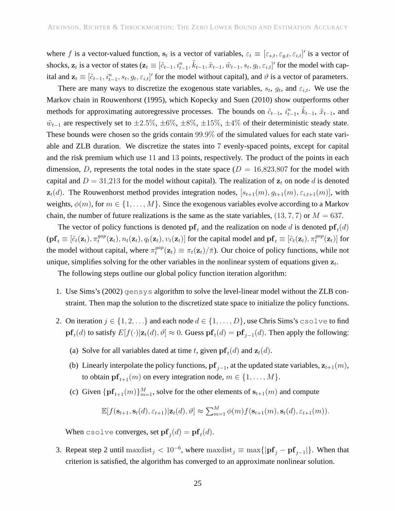
B NONLINEAR SOLUTION METHOD
We begin by compactly writing the detrended nonlinear equilibrium system as
E[f(st+1, st, εt+1)|zt, ϑ] = 0,
24
ATKINSON, RICHTER & T HROCKMORTON: THE ZERO LOWER BOUND AND ESTIMATION ACCURACY
wheref is a vector-valued function,st is a vector of variables,εt ≡ [εs,t, εg,t, εi,t]′ is a vector of
shocks,zt is a vector of states (zt ≡ [ct−1, int−1, kt−1, xt−1, wt−1, st, gt, εi,t]
′ for the model with cap-
ital andzt ≡ [ct−1, int−1, st, gt, εi,t]
′ for the model without capital), andϑ is a vector of parameters.
There are many ways to discretize the exogenous state variables,st, gt, andεi,t. We use the
Markov chain in Rouwenhorst (1995), which Kopecky and Suen (2010) show outperforms other
methods for approximating autoregressive processes. The bounds onct−1, int−1, kt−1, xt−1, and
wt−1 are respectively set to±2.5%, ±6%, ±8%, ±15%, ±4% of their deterministic steady state.
These bounds were chosen so the grids contain99.9% of the simulated values for each state vari-
able and ZLB duration. We discretize the states into7 evenly-spaced points, except for capital
and the risk premium which use11 and13 points, respectively. The product of the points in each
dimension,D, represents the total nodes in the state space (D = 16,823,807 for the model with
capital andD = 31,213 for the model without capital). The realization ofzt on noded is denoted
zt(d). The Rouwenhorst method provides integration nodes,[st+1(m), gt+1(m), εi,t+1(m)], with
weights,φ(m), for m ∈ {1, . . . ,M}. Since the exogenous variables evolve according to a Markov
chain, the number of future realizations is the same as the state variables,(13, 7, 7) orM = 637.
The vector of policy functions is denotedpf t and the realization on noded is denotedpf t(d)
(pf t ≡ [ct(zt), πgapt (zt), nt(zt), qt(zt), υt(zt)] for the capital model andpf t ≡ [ct(zt), π
gapt (zt)] for
the model without capital, whereπgapt (zt) ≡ πt(zt)/π). Our choice of policy functions, while not
unique, simplifies solving for the other variables in the nonlinear system of equations givenzt.
The following steps outline our global policy function iteration algorithm:
1. Use Sims’s (2002)gensys algorithm to solve the level-linear model without the ZLB con-
straint. Then map the solution to the discretized state space to initialize the policy functions.
2. On iterationj ∈ {1, 2, . . .} and each noded ∈ {1, . . . , D}, use Chris Sims’scsolve to find
pf t(d) to satisfyE[f(·)|zt(d), ϑ] ≈ 0. Guesspf t(d) = pf j−1(d). Then apply the following:
(a) Solve for all variables dated at timet, givenpf t(d) andzt(d).
(b) Linearly interpolate the policy functions,pf j−1, at the updated state variables,zt+1(m),
to obtainpf t+1(m) on every integration node,m ∈ {1, . . . ,M}.
(c) Given{pf t+1(m)}Mm=1, solve for the other elements ofst+1(m) and compute
E[f(st+1, st(d), εt+1)|zt(d), ϑ] ≈∑M
m=1 φ(m)f(st+1(m), st(d), εt+1(m)).
Whencsolve converges, setpf j(d) = pf t(d).
3. Repeat step 2 untilmaxdistj < 10−6, wheremaxdistj ≡ max{|pf j − pf j−1|}. When that
criterion is satisfied, the algorithm has converged to an approximate nonlinear solution.
25
ATKINSON, RICHTER & T HROCKMORTON: THE ZERO LOWER BOUND AND ESTIMATION ACCURACY
C ESTIMATION ALGORITHM
We use a random walk Metropolis-Hastings algorithm to estimate the model insection 3with
artificial data of120 quarters. To measure how well the model fits the data, we use either the
adapted particle filter described in Algorithm 14 in Herbst and Schorfheide (2016), which modifies
the basic bootstrap filter in Stewart and McCarty (1992) and Gordon et al. (1993) to better account
for the outliers in the data, or the inversion filter recentlyused by Guerrieri and Iacoviello (2017).
C.1 METROPOLIS-HASTINGS ALGORITHM The following steps outline the algorithm:
1. Generate artificial data consisting of the output growth gap, the inflation rate, and the nomi-
nal interest rate,xt ≡ [ygt , πt, it]′, whereNx = 3 is the number of observable variables.
2. Specify the prior distributions, means, variances, and bounds of each element of the vector
of Ne estimated parameters,θ ≡ [ϕp, φπ, φy, h, ρs, ρi, σg, σs, σi]′.
3. Find the posterior mode to initialize the preliminary Metropolis-Hastings step.
(a) For alli ∈ {1, . . . , Nm}, whereNm = 5,000, apply the following steps:
i. Draw θi from the joint prior distribution and calculate its densityvalue:
log ℓpriori =∑Ne
j=1 log p(θi,j|µj, σ2j ),
wherep is the prior density function of parameterj with meanµj and varianceσ2j .
ii. Solve the model givenθi. Follow Appendix Bfor the nonlinear model and use
OccBin for the PW linear model. Repeat 3(a)i if the algorithmdoes not converge.
iii. Obtain the model log-likelihood,log ℓmodeli . Apply the particle filter described in
section C.2to the nonlinear model and the inversion filter to the PW linear model.
iv. The posterior log-likelihood islog ℓposti = log ℓpriori + log ℓmodeli
(b) Calculatemax(log ℓpost1 , . . . , log ℓpostNm) and find the corresponding parameter vector,θ0.
4. Approximate the covariance matrix for the joint posterior distribution of the parameters,Σ,
which is used to obtain candidate draws during the preliminary Metropolis-Hastings step.
(a) Locate the draws with a likelihood in the top decile. Stack theNm,sub = (1 − p)Nm
draws in aNm,sub ×Ne matrix,Θ, and defineΘ = Θ−∑Nm,sub
i=1 θi,j/Nm,sub.
(b) CalculateΣ = Θ′Θ/Nm,sub and verify it is positive definite, otherwise repeat step 3.
5. Perform an initial run of the random walk Metropolis-Hastings algorithm.
26

ATKINSON, RICHTER & T HROCKMORTON: THE ZERO LOWER BOUND AND ESTIMATION ACCURACY
(a) For alli ∈ {0, . . . , Nd}, whereNd = 25,000, perform the following steps:
i. Draw a candidate vector of parameters,θcandi , where
θicand ∼
N(θ0, c0Σ) for i = 0,
N(θi−1, cΣ) for i > 0.
We setc0 = 0 and tunec to target an overall acceptance rate of roughly30%.
ii. Calculate the prior density value,log ℓpriori , of the candidate draw,θcandi , as in 3(a)i.
iii. Solve the model givenθcandi . If the algorithm does not converge repeat 5(a)i.
iv. Obtain the model log-likelihood value,log ℓmodeli , using the methods in 3(a)iii.
v. Accept or reject the candidate draw according to
(θi, log ℓi) =
(θcandi , log ℓcandi ) if i = 0,
(θcandi , log ℓcandi ) if min(1, ℓcandi /ℓi−1) > u,
(θi−1, log ℓi−1) otherwise,
where u is a draw from a uniform distribution,U[0, 1], and the posterior log-
likelihood associated with the candidate draw islog ℓcandi = log ℓpriori + log ℓmodeli .
(b) Burn the firstNb = 5000 draws and use the remaining sample to calculate the mean
draw,θ5(b) =∑Nd
i=Nb+1 θi/(Nd −Nb), and the covariance matrix,Σ5(b). We follow step
4 to calculateΣ5(b) but use allNd −Nb draws instead of just the upperpth percentile.
6. Conduct a final run of the Metropolis-Hastings algorithm by repeating step 5, whereNd =
50,000, θ0 = θ5(b), andΣ = Σ5(b). The final posterior mean estimates areθ =∑Nd
i=1 θi/Nd.
C.2 ADAPTED PARTICLE FILTER Henceforth, our definition ofst from Appendix Bis referred
to as the state vector, which should not be confused with the state variables for the nonlinear model.
1. Initialize the filter by drawing{εt,p}0t=−24 for all p ∈ {0, . . . , Np} and simulating the model,
whereNp is the number of particles. We initialize the filter with the final state vector,s0,p,
which is approximately a draw from the model’s ergodic distribution. We setNp = 40,000.
2. Fort ∈ {1, . . . , T}, sequentially filter the nonlinear model as follows:
(a) Forp ∈ {1, . . . , Np}, draw shocks from an adapted distribution,εt,p ∼ N(εt, I), where
εt maximizesp(ξt|st)p(st|st−1) andst−1 =∑Np
p=1 st−1,p/Np is the mean state vector.
i. Use the model solution to update the state vector,st, givenst−1 and a guess forεt.
Definesht ≡ Hst, whereH selects the observable variables from the state vector.
27

ATKINSON, RICHTER & T HROCKMORTON: THE ZERO LOWER BOUND AND ESTIMATION ACCURACY
ii. Calculate the measurement error,ξt = sht −xt, which is assumed to be multivariate
normally distributed,p(ξt|st) = (2π)−3/2|R|−1/2 exp(−ξ′tR−1ξt/2), whereR ≡
diag(σ2me,yg , σ
2me,π, σ
2me,i) is a diagonal matrix of measurement error variances.
iii. The probability of observing the current state,st, conditional onst−1, is given by
p(st|st−1) = (2π)−3/2 exp(−ε′tεt/2).
iv. Maximizep(ξt|st)p(st|st−1) ∝ exp(−ξ′tR−1ξt/2) exp(−ε′tεt/2) by solving for the
optimalεt. We use MATLAB’sfminsearch routine converted to Fortran.
(b) Use the model solution to predict the state vector,st,p, givenst−1,p andεt,p.
(c) Calculateξt,p = sht,p − xt. The unnormalized weight on particlep is given by
ωt,p =p(ξt|st,p)p(st,p|st−1,p)
g(st,p|st−1,p,xt)∝
exp(−ξ′t,pR−1ξt,p/2) exp(−ε′t,pεt,p/2)
exp(−(εt,p − εt)′(εt,p − εt)/2).
Without adaptation,εt = 0 andωt,p = p(ξt|st,p), as in a basic bootstrap particle filter.
The time-t contribution to the model log-likelihood isℓmodelt =
∑Np
p=1 ωt,p/Np.
(d) Normalize the weights,Wt,p = ωt,p/∑Np
p=1 ωt,p. Then use systematic resampling with
replacement from the swarm of particles as described in Kitagawa (1996) to get a set
of particles that represents the filter distribution and reshuffle{st,p}Np
p=1 accordingly.
3. The model log-likelihood islog ℓmodel =∑T
t=1 log ℓmodelt .
Aruoba et al. (2018) apply the same methodology to a New Keynesian model with sunspot shocks.
See Herbst and Schorfheide (2016) for a comprehensive discussion of the different particle filters.
D CONTINUOUS RANK PROBABILITY SCORE (CRPS) EXAMPLE
Figure 5shows an example of the 8-quarter ahead forecast distribution of the nominal interest rate
given the parameter estimates from NL-PF-5%. We picked a dataset where the ZLB binds for six
quarters, from period90 to 95 in the sample. The forecasts are initialized at the filtered state in
period89, immediately before the ZLB first binds, and the forecast distribution is approximated
based on10,000 simulations. Due to a strong tendency for the forecasts to revert to the stochastic
steady state, the mean forecast for the nominal interest rate is 2.32%. However, the probability
density function (PDF) in the left panel shows a significant number of forecasts remain near or at
the ZLB, even after 8 quarters. The true realization equals1.94%, which means there is signifi-
cant probability mass under the PDF above and below the true value. The right panel shows the
cumulative distribution function (CDF) of the forecasts. TheCRPS for this dataset and estimation
method is closely related to the shaded area, which has the same units as the forecasted variable.
28

ATKINSON, RICHTER & T HROCKMORTON: THE ZERO LOWER BOUND AND ESTIMATION ACCURACY
0 2 4 6 80
0.05
0.1
0.15
0.2
0.25
0.3
0 2 4 6 80
0.2
0.4
0.6
0.8
1
Truth
Truth
Figure 5: Example forecast distribution in the period before the ZLB binds in the data.
E ADDITIONAL RESULTS
The section provides additional results. First, we show theeffects of reducing misspecification
by estimating a richer piecewise linear model. Second, we show how misspecification affects the
parameter estimates and recession responses by generatingdata from our small-scale model. Third,
we plot impulse responses to a technology growth and monetary policy shock when the ZLB binds.
E.1 LARGER ESTIMATED MODEL Table 7shows how the PW-IF-0% parameter estimates are
affected when sticky wages are included in the estimated model to reduce the amount of model
misspecification. The equilibrium system is the same as the original small-scale model, except
(43) and (44) are replaced with (28), (32), (40), and a definition of real GDP that accounts for
the resources lost due to sticky wages (i.e.,ygdpt = [1 − ϕp(πt/π − 1)2/2 − ϕw(wgt − 1)2/2]yt).
Sticky wages would add another state variable and substantially increase the computational cost
of NL-PF-5%. In particular, the new state variable would increase the solution time by the percent
increase in the state space plus the additional time it takeson each node to interpolate in that
dimension. The first two columns show the NL-PF-5% and PW-IF-0% estimates using the original
estimated model and the last column shows the PW-IF-0% estimates in the less misspecified model.
In datasets with a 30 quarter ZLB event, introducing sticky wages reduces the sum of the
NRMSE from 1.91 to 1.59, creating a clear advantage over NL-PF-5%. This result is driven by
more accurate estimates ofϕp andh, which dominate the lower accuracy ofσs. Our other accuracy
measures also improve. Estimates of the expected ZLB duration and probability of a 4-quarter ZLB
event become more accurate and essentially unbiased. The PW-IF-0% CRPS is now lower than
the NL-PF-5% CRPS at a 4-quarter horizon and the NL-PF-5% advantage at an 8-quarter horizon
is smaller. These results suggest it is better to apply PW-IF-0% to a less misspecified model than
29
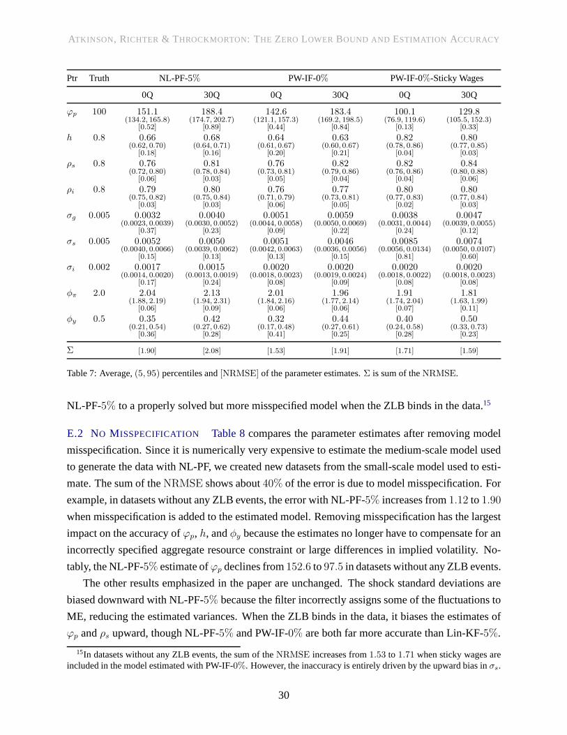
ATKINSON, RICHTER & T HROCKMORTON: THE ZERO LOWER BOUND AND ESTIMATION ACCURACY
Ptr Truth NL-PF-5% PW-IF-0% PW-IF-0%-Sticky Wages
0Q 30Q 0Q 30Q 0Q 30Q
ϕp 100 151.1 188.4 142.6 183.4 100.1 129.8(134.2, 165.8) (174.7, 202.7) (121.1, 157.3) (169.2, 198.5) (76.9, 119.6) (105.5, 152.3)
[0.52] [0.89] [0.44] [0.84] [0.13] [0.33]
h 0.8 0.66 0.68 0.64 0.63 0.82 0.80(0.62, 0.70) (0.64, 0.71) (0.61, 0.67) (0.60, 0.67) (0.78, 0.86) (0.77, 0.85)
[0.18] [0.16] [0.20] [0.21] [0.04] [0.03]
ρs 0.8 0.76 0.81 0.76 0.82 0.82 0.84(0.72, 0.80) (0.78, 0.84) (0.73, 0.81) (0.79, 0.86) (0.76, 0.86) (0.80, 0.88)
[0.06] [0.03] [0.05] [0.04] [0.04] [0.06]
ρi 0.8 0.79 0.80 0.76 0.77 0.80 0.80(0.75, 0.82) (0.75, 0.84) (0.71, 0.79) (0.73, 0.81) (0.77, 0.83) (0.77, 0.84)
[0.03] [0.03] [0.06] [0.05] [0.02] [0.03]
σg 0.005 0.0032 0.0040 0.0051 0.0059 0.0038 0.0047(0.0023, 0.0039) (0.0030, 0.0052) (0.0044, 0.0058) (0.0050, 0.0069) (0.0031, 0.0044) (0.0039, 0.0055)
[0.37] [0.23] [0.09] [0.22] [0.24] [0.12]
σs 0.005 0.0052 0.0050 0.0051 0.0046 0.0085 0.0074(0.0040, 0.0066) (0.0039, 0.0062) (0.0042, 0.0063) (0.0036, 0.0056) (0.0056, 0.0134) (0.0050, 0.0107)
[0.15] [0.13] [0.13] [0.15] [0.81] [0.60]
σi 0.002 0.0017 0.0015 0.0020 0.0020 0.0020 0.0020(0.0014, 0.0020) (0.0013, 0.0019) (0.0018, 0.0023) (0.0019, 0.0024) (0.0018, 0.0022) (0.0018, 0.0023)
[0.17] [0.24] [0.08] [0.09] [0.08] [0.08]
φπ 2.0 2.04 2.13 2.01 1.96 1.91 1.81(1.88, 2.19) (1.94, 2.31) (1.84, 2.16) (1.77, 2.14) (1.74, 2.04) (1.63, 1.99)
[0.06] [0.09] [0.06] [0.06] [0.07] [0.11]
φy 0.5 0.35 0.42 0.32 0.44 0.40 0.50(0.21, 0.54) (0.27, 0.62) (0.17, 0.48) (0.27, 0.61) (0.24, 0.58) (0.33, 0.73)
[0.36] [0.28] [0.41] [0.25] [0.28] [0.23]
Σ [1.90] [2.08] [1.53] [1.91] [1.71] [1.59]
Table 7: Average,(5, 95) percentiles and[NRMSE] of the parameter estimates.Σ is sum of theNRMSE.
NL-PF-5% to a properly solved but more misspecified model when the ZLB binds in the data.15
E.2 NO M ISSPECIFICATION Table 8compares the parameter estimates after removing model
misspecification. Since it is numerically very expensive toestimate the medium-scale model used
to generate the data with NL-PF, we created new datasets fromthe small-scale model used to esti-
mate. The sum of theNRMSE shows about40% of the error is due to model misspecification. For
example, in datasets without any ZLB events, the error with NL-PF-5% increases from1.12 to 1.90
when misspecification is added to the estimated model. Removing misspecification has the largest
impact on the accuracy ofϕp, h, andφy because the estimates no longer have to compensate for an
incorrectly specified aggregate resource constraint or large differences in implied volatility. No-
tably, the NL-PF-5% estimate ofϕp declines from152.6 to97.5 in datasets without any ZLB events.
The other results emphasized in the paper are unchanged. Theshock standard deviations are
biased downward with NL-PF-5% because the filter incorrectly assigns some of the fluctuations to
ME, reducing the estimated variances. When the ZLB binds in the data, it biases the estimates of
ϕp andρs upward, though NL-PF-5% and PW-IF-0% are both far more accurate than Lin-KF-5%.
15In datasets without any ZLB events, the sum of theNRMSE increases from1.53 to 1.71 when sticky wages areincluded in the model estimated with PW-IF-0%. However, the inaccuracy is entirely driven by the upward bias inσs.
30

ATKINSON, RICHTER & T HROCKMORTON: THE ZERO LOWER BOUND AND ESTIMATION ACCURACY
No Misspecification: DGP and Estimation Use Small-Scale ModelPtr Truth NL-PF-5% PW-IF-0% Lin-KF-5%
0Q 30Q 0Q 30Q 0Q 30Q
ϕp 100 96.8 109.8 94.3 110.6 103.7 128.5(81.6, 109.9) (89.5, 130.3) (81.8, 108.3) (95.3, 125.1) (92.6, 118.4) (111.2, 145.3)
[0.09] [0.15] [0.11] [0.15] [0.09] [0.30]
h 0.8 0.79 0.79 0.79 0.79 0.80 0.79(0.76, 0.82) (0.77, 0.82) (0.75, 0.82) (0.77, 0.82) (0.76, 0.83) (0.76, 0.82)
[0.02] [0.02] [0.02] [0.02] [0.02] [0.03]
ρs 0.8 0.80 0.83 0.81 0.84 0.82 0.87(0.76, 0.83) (0.78, 0.86) (0.76, 0.85) (0.80, 0.87) (0.77, 0.86) (0.83, 0.91)
[0.03] [0.04] [0.04] [0.06] [0.05] [0.10]
ρi 0.8 0.82 0.82 0.79 0.79 0.82 0.86(0.79, 0.84) (0.78, 0.85) (0.77, 0.82) (0.74, 0.82) (0.79, 0.84) (0.83, 0.88)
[0.03] [0.03] [0.02] [0.03] [0.03] [0.08]
σg 0.005 0.0037 0.0035 0.0051 0.0052 0.0038 0.0034(0.0029, 0.0046) (0.0025, 0.0045) (0.0044, 0.0056) (0.0043, 0.0061) (0.0029, 0.0046) (0.0026, 0.0044)
[0.27] [0.33] [0.08] [0.11] [0.26] [0.33]
σs 0.005 0.0047 0.0043 0.0049 0.0046 0.0047 0.0036(0.0035, 0.0058) (0.0032, 0.0058) (0.0039, 0.0060) (0.0034, 0.0057) (0.0034, 0.0059) (0.0027, 0.0046)
[0.19] [0.22] [0.16] [0.17] [0.21] [0.32]
σi 0.002 0.0016 0.0014 0.0020 0.0019 0.0016 0.0015(0.0013, 0.0020) (0.0010, 0.0018) (0.0017, 0.0022) (0.0016, 0.0022) (0.0013, 0.0019) (0.0012, 0.0017)
[0.20] [0.31] [0.07] [0.10] [0.20] [0.27]
φπ 2.0 2.00 2.01 1.95 1.80 1.97 1.62(1.81, 2.21) (1.82, 2.20) (1.74, 2.14) (1.58, 2.06) (1.76, 2.18) (1.42, 1.86)
[0.06] [0.06] [0.06] [0.12] [0.07] [0.20]
φy 0.5 0.45 0.48 0.46 0.52 0.46 0.50(0.29, 0.61) (0.28, 0.61) (0.30, 0.63) (0.32, 0.73) (0.31, 0.63) (0.34, 0.66)
[0.22] [0.18] [0.21] [0.23] [0.22] [0.19]
Σ [1.12] [1.35] [0.78] [0.99] [1.14] [1.82]
Table 8: Average,(5, 95) percentiles and[NRMSE] of the parameter estimates.Σ is sum of theNRMSE.
Figure 6plots the recession responses infigure 3without misspecification. The solid line shows
the responses based on the true parameterization of the small-scale model, rather than the medium-
scale model that generates our original datasets. The dashed line shows the mean responses, given
the parameter estimates with our alternative datasets. Consistent with the previous results, the re-
sponses based on the NL-PF-5% and PW-IF-0% parameter estimates are very similar. The key dif-
ference is that the mean estimated simulations are much closer to the true simulation and the(5, 95)
percentiles almost always encompass the truth. This resultshows the muted responses infigure 3
are primarily driven by model misspecification, rather thaninaccuracies in the estimation methods.
E.3 IMPULSE RESPONSES This section shows generalized impulse response functions(GIRFs)
of a technology growth and monetary policy shock when the economy is in a severe recession and
the ZLB binds. To compute the GIRFs, we follow Koop et al. (1996). We first calculate the mean
of 10,000 simulations, conditional on random shocks in every quarter(i.e., the baseline path). We
then calculate a second mean from another set of10,000 simulations, but this time the shock in
the first quarter is replaced with a two standard deviation negative technology growth or monetary
policy shock (i.e., the impulse path). Finally, we plot the differences between the two mean paths.
31

ATKINSON, RICHTER & T HROCKMORTON: THE ZERO LOWER BOUND AND ESTIMATION ACCURACY
0 2 4 6 8 10 12 14 16 18 20-6
-4
-2
0
2
4
0 2 4 6 8 10 12 14 16 18 20-6
-4
-2
0
2
4
0 2 4 6 8 10 12 14 16 18 20-6
-4
-2
0
2
4
0 2 4 6 8 10 12 14 16 18 20-6
-4
-2
0
2
4
0 2 4 6 8 10 12 14 16 18 20-6
-4
-2
0
2
4
0 2 4 6 8 10 12 14 16 18 20-6
-4
-2
0
2
4
Figure 6: Recession responses without misspecification. The solid line is the true simulation, the dashed line is themean estimated simulation, and the shaded area contains the(5, 95) percentiles across the datasets. The simulationsare initialized in steady state and followed by four1.5 standard deviation positive risk premium shocks.
The benefit of a GIRF over a traditional impulse response function is that it allows us to calcu-
late the responses in any state of the economy without the influence of mean reversion. For the true
model, we initialize at the state following four consecutive1.5 standard deviation positive risk pre-
mium shocks, consistent withfigure 3. We then find a sequence of four equally sized risk premium
shocks that produce the same notional rate in our estimated model as the true model, so the simula-
tions begin at the same point. The NL-PF-5% simulations are shown in the left column and the PW-
IF-0% simulations are in the right column. The true simulation of the DGP (solid line) is compared
to the mean estimated simulation of the small-scale model (dashed line). The(5, 95) percentiles
account for the differences in the simulations across the parameter estimates for each dataset.
32

ATKINSON, RICHTER & T HROCKMORTON: THE ZERO LOWER BOUND AND ESTIMATION ACCURACY
0 4 8 12 16
-1
-0.8
-0.6
-0.4
-0.2
0
0 4 8 12 16-2
-1.5
-1
-0.5
0
0 4 8 12 16-0.1
0
0.1
0.2
0.3
0.4
0 4 8 12 16-0.1
0
0.1
0.2
0.3
0.4
0 4 8 12 16-0.2
-0.15
-0.1
-0.05
0
0.05
0 4 8 12 16-0.2
-0.15
-0.1
-0.05
0
0.05
Figure 7: Responses to a -2 standard deviation technology growth shock in a severe recession. The solid line is thetrue simulation, the dashed line is the mean estimated simulation, and the shaded area contains the(5, 95) percentiles.
Figure 7shows the responses to a technology growth shock. Qualitatively the responses of out-
put growth and inflation are similar across the specifications. Higher technology growth increases
the output growth gap and decreases the inflation rate like a typical supply shock. Since the Fed
faces a tradeoff between stabilizing the inflation and output gaps, the notional interest rate response
depends on the parameterization. The notional rate rises with the DGP, but falls with both of the
estimated models. Quantitatively, there are important differences between all of the responses.
Consistent withfigure 3, model misspecification leads to muted responses of the output growth
gap and the inflation rate. There are also differences in the magnitudes of the estimated responses,
but most of that is driven by the downward bias in the shock standard deviation with NL-PF-5%.
33

ATKINSON, RICHTER & T HROCKMORTON: THE ZERO LOWER BOUND AND ESTIMATION ACCURACY
0 4 8 12 16-0.2
0
0.2
0.4
0.6
0.8
0 4 8 12 16
0
0.2
0.4
0.6
0.8
1
0 4 8 12 160
0.1
0.2
0.3
0.4
0 4 8 12 160
0.1
0.2
0.3
0.4
0.5
0 4 8 12 16-1.5
-1
-0.5
0
0 4 8 12 16-2
-1.5
-1
-0.5
0
Figure 8: Responses to a -2 standard deviation monetary policy shock in a severe recession. The solid line is the truesimulation, the dashed line is the mean estimated simulation, and the shaded area contains the(5, 95) percentiles.
Figure 8shows the responses to a monetary policy shock. Although theZLB binds in the true
and estimated models, the shock is expansionary because it lowers the expected nominal interest
rate in future periods. Therefore, the output growth gap andthe inflation rate both increase in
all three models. Unlike with the other two shocks, model misspecification has a relatively small
effect on the responses, as the(5, 95) percentiles of the estimated responses encompass the true
responses in most periods. There are some differences in theNL-PF-5% and PW-IF-0% responses,
but they are smaller than infigure 7and never large enough to have meaningful policy implications.
34